Coupling Online-Offline Learning for Multi-distributional Data Streams

Abstract

The distributions of real-life data streams are usually nonstationary, where one exciting setting is that a stream can be decomposed into several offline intervals with a fixed time horizon but different distributions and an out-of-distribution online interval. We call such data multi-distributional data streams, on which learning an on-the-fly expert for unseen samples with a desirable generalization is demanding yet highly challenging owing to the multi-distributional streaming nature, particularly when initially limited data is available for the online interval. To address these challenges, this work introduces a novel optimization method named coupling online-offline learning (CO₂) with theoretical guarantees about the knowledge transfer, the regret, and the generalization error. CO₂ extracts knowledge by training an offline expert for each offline interval and update an online expert by an off-the-shelf online optimization method in the online interval. CO₂ outputs a hypothesis for each sample by adaptively coupling both the offline experts and the underlying online expert through an expert-tracking strategy to adapt to the dynamic environment. To study the generalization performance of the output hypothesis, we propose a general theory to analyze its excess risk bound related to the loss function properties, the hypothesis class, the data distribution, and the regret.

Keywords: Nonstationary, Coupling, Generalization

A common assumption of statistical learning theories for data streams is that the observed samples are i.i.d., which is also referred to as stationary in stochastic processes (Hamilton, 1994). Based on that, to exploit the inherent sample dependence, a widely-applied assumption for actual non-i.i.d. processes is to assume that observations are drawn from a stationary $\phi$-mixing or $\beta$-mixing sequence (Mohri and Rostamizadeh, 2010). However, the stationary and mixing assumptions may not hold because the distribution of real-life streaming data usually changes over time, and samples from arbitrary distributions will cause the defined hypothesis class to be not (agnostically) PAC learnable (Hanneke, 2016) since increasing the number of training samples still leads to a random hypothesis. Fortunately, as assumed by Kuznetsov and Mohri (2015), the change of distributions in real life is often not drastic, and samples in a short interval are almost sampled from an identical distribution.

Building on the above discussion, we consider a more general and realistic scenario about nonstationary non-mixing sequences, named multi-distributional data streams. We assume a general setting of a multi-distributional data stream as follows. It consists of several offline intervals with different distributions in a fixed offline time horizon and an out-of-distribution online interval that constantly receives new samples. After the number of received labeled samples reaches the predefined size, the online interval is converted to be the last offline interval and a new online interval appears. The online interval expert is updated according to the loss from labeled samples and predicts the class labels for unlabeled samples.

The first baseline is to train an expert on the entire data stream by applying an off-the-shelf online optimization method (Shalev-Shwartz, 2012) without considering the multi-distributional streaming nature. However, the dynamic data with various distributions will mislead the expert. Although the second method, learning an expert from scratch for a new out-of-distribution online interval, is safe, the rare labeled samples at the early stage will induce an unreliable expert. Therefore, it is fundamental yet highly challenging to design a learning method with tight sample complexity to output a hypothesis with desirable generalization for such multi-distributional data streams.

To manage the challenge in the second method when training a reliable and efficient expert, one way is to exploit previous offline intervals since they with all observed samples are transparent, where some of their distributions may be similar to that of the online interval. Accordingly, the first question is how to extract the prior knowledge from offline intervals? Although one may assume this question could be addressed by techniques like transfer learning (Zhao et al., 2014), which are actually inapplicable since the online interval in our setting differs from a target domain for the knowledge transfer and is not fully observed. The second question is how to adapt an off-the-shelf online optimization method on the multi-distributional data stream to train an expert with extracted knowledge? The expert is trained on the fly, and the traditional regret theory of analyzing the performance of an online method focuses on observed labeled samples. Also, most of the existing studies (Yu, 1994; Mohri and Rostamizadeh, 2008, 2010) about generalization bound for data streams are based on the stationarity and mixing assumptions for an offline setting but ignore the particular optimization method used. However, the applied optimization method has a significant impact on analyzing the bound because the gap between the empirical minimizer and the output solution may be large in an online setting. Accordingly, the last question is how to establish the generalization bound of the learned output solution if an online optimization method is given? To address the above questions, we propose a novel Coupling Online-Offline learning (CO₂) method with theoretical guarantees.

To answer the first question, we maintain several offline experts learned from previous offline intervals and update an online expert on the out-of-distribution online interval. More specifically, when an online interval becomes outdated, i.e., offline, all samples of this interval are used to train a new offline expert, and the oldest offline expert is discarded. The corresponding online expert with access to each sample once and the previous offline experts learned from previous intervals can offer reference values for training the newly-added offline expert. Accordingly, we transfer the knowledge learned from all maintained experts by restricting its search space. Theoretically, the gap between the empirical minimizer and the optimal solution is proportional to the maintained experts’ empirical errors on this interval. Therefore, we adaptively weight these experts according to their effects to narrow the gap (c.f. Theorem 4).

Our response to the second question is below: the proposed CO₂ method learns a meta-expert in the current out-of-distribution online interval. It combines the online and offline experts adaptively with an expert-tracking strategy, where the online expert is trained by an off-the-shelf online optimization method. The meta-expert follows the paradigm of prediction with expert advice (Cesa-Bianchi and Lugosi, 2006) and is inspired by the strategy of maintaining different experts with various learning rates in MetaGrad (van Erven and Koolen, 2016). We prove the regret of CO₂ is determined by that of the used off-the-shelf online optimization method for the online expert but can be improved if the number of the maintained experts is within the bound controlled by the size of intervals and the empirical errors of the maintained experts (c.f. Theorem 5).

For the last question, we imply the generalization by the regret of the proposed CO₂ method. By extending the previous study (Hazan, 2016) of connecting optimization with learning theory, we establish a more precise excess risk bound for the output solution of CO₂ by jointly exploiting its regret, the loss function properties, the hypothesis class, and the data distribution, and further analyze its bottlenecks (c.f. Theorem 10).

The outline of the paper is as follows. In Section 1, we review some existing work related to our model design as well as theoretical analysis. In Section 2, we describe the proposed CO₂ algorithm in detail. In Section 3, we show our main results concerning the theoretical guarantees. We defer the detailed proofs to the supplementary material.

1 Related Work

In this section, we provide a brief review of the related work.

1.1 Learning in Dynamic Environments

One of the popular classic statistical models for handling dynamic time series-based streams is the autoregressive moving average (ARMA). However, ARMA and its integrated version ARIMA (Yang, 2005) and other improved versions (Hamilton, 1994; Csáji, 2016) rely heavily on the assumption that the error terms are i.i.d. drawn from a normal distribution with zero mean value. To adapt to a nonstationary environment, a state-of-the-art approach (Kuznetsov and Mohri, 2015) learns sample weights according to training errors with the prior knowledge that the fresh samples share larger weights than previous. However, this approach cannot be applied to an online setting because it needs to calculate each new sample’s weight by accessing the entire database.

For online optimization methods, the regret theory (Buchbinder et al., 2016) for measuring the performance has been extensively studied. The dynamic regret (Zinkevich, 2003) and its restricted form (Besbes et al., 2015) have been introduced to manage changing environments. A basic idea behind such regrets is to compare the learned expert’s cumulative loss with several experts rather than the best one. Along this line of study, adaptive learning for dynamic regret (Ader) (Zhang et al., 2018) considers multiple experts with various learning rates updated by online gradient descent (OGD) (Zinkevich, 2003), and the established upper bound matches the lower bound. Another independent work for dynamic regret in a nonstationary environment is about multi-armed bandit (MAB) (Besbes et al., 2015), where the work in (Wei et al., 2019) reveals how the statistical variance of the loss distributions affect the dynamic regret bound. However, these dynamic regrets depend on the distribution changing times, which are usually unknown. When the sequence of samples is very long, the data distribution may have changed many times. As a result, the loose bound cannot measure the learned expert’s performance in the current interval. Another limitation is that the bound is inappropriate for analyzing experts learned on the fly because these regrets only act on observed samples.

1.2 Learning Theory for Data Streams

For non-i.i.d. processes, under the stationary and $\beta$-mixing assumptions, the early work (Yu, 1994) establishes the convergence rate over VC-dimension, and the work in Mohri and Rostamizadeh (2008) presents data-dependent bounds in terms of the Rademacher complexity. By exploiting a specific learning algorithm’s stability properties, generalization bounds for $\phi$-mixing and $\beta$-mixing sequences are provided in Mohri and Rostamizadeh (2010). However, the mixing assumption is hard to be verified in practice.

There are some attempts to relax the stationary and mixing assumptions. The uniform convergence under ergodicity sampling is shown in the work of Adams and Nobel (2010). For an asymptotically stationary (mixing) process, although a generalization error is derived in Agarwal and Duchi (2013) through the regret of an online algorithm, and their analysis depends on the assumption that the output from an online learning algorithm tends to be stable, which is invalid in a dynamic environment. In Kuznetsov and Mohri (2014), the guarantee of the learning rate for nonstationary mixing processes is given by a sub-sample selection technique with the Rademacher complexity. Further, the convergence rate for sequential samples without mixing or ergodicity assumptions is established in Rakhlin et al. (2015) by applying the sequential Rademacher complexity, which can be bounded by a Dudley’s integral in terms of covering number (Zhang, 2002) through the chaining technique. In Kuznetsov and Mohri (2015), a more general scenario of nonstationary and non-mixing processes is considered, which proves the learning guarantees with the conditions of the discrepancies between distributions.

2 Our CO₂ Method

After introducing several common assumptions, we then present the proposed CO₂ method in detail. Inspired by the adaptive online learning algorithm MetaGrad (van Erven and Koolen, 2016), CO₂ maintains several offline experts for the corresponding offline intervals and an online expert for the current online interval and then integrates all of these experts by a meta-expert.

2.1 Assumptions

We assume there are $G$ intervals: $G-1$ offline intervals, and an online interval.

Assumption 1

Let $\mathcal{D}_{g}$ be the data distribution in the $g^{\text{th}}$ interval and $\mathcal{D}_{\mathcal{U}}=\bigcup_{g=1}^{G}\mathcal{D}_{g}$ be the mixture distribution, the distributions in a multi-distributional data stream are nonstationary, i.e.,

$$\mathcal{D}_{g}\neq\mathcal{D}_{g^{\prime}},\forall g,g^{\prime}\in[G],g\neq g^{\prime}.$$

Assumption 2

The norm of every input sample $\mathbf{x}$ with label $y$ in the Hilbert space i.i.d. drawn from the distribution $\mathcal{D}_{G}$ of the online interval is upper bounded by a constant $D$:

$$\|\mathbf{x}\|\leq D,\forall(\mathbf{x},y)\thicksim\mathcal{D}_{G}.$$

The eigendecomposition of the Hilbert-Schmidt operator is

$$\mathbb{E}_{(\mathbf{x},y)\thicksim\mathcal{D}_{G}}[\mathbf{x}\mathbf{x}^{T}]=\sum_{i=1}^{\infty}\lambda_{i}\mathbf{u}_{i}\mathbf{u}_{i}^{T}$$

where $(\mathbf{u}_{i})_{i=1}^{\infty}$ forms an orthonormal basis of Hilbert Space and $(\lambda_{i})_{i=1}^{\infty}$ corresponds to the eigenvalues in a non-increasing order.

Assumption 3

For any sample $(\mathbf{x},y)\thicksim\mathcal{D}_{\mathcal{U}}$, the hypothesis class is

$$\mathcal{H}\triangleq\{h:\mathbf{x}\mapsto\left<\mathbf{w},\mathbf{x}\right>\,|\,\mathbf{w}\in\mathcal{W},\|\mathbf{w}\|\leq R\}$$

where the domain $\mathcal{W}$ bounded by $R$ is a convex subspace of a Hilbert space.

Assumption 4

For any sample $(\mathbf{x},y)\thicksim\mathcal{D}_{\mathcal{U}}$, the loss function family $\mathcal{L}$ with the hypothesis class $\mathcal{H}$ is bounded in the interval $[0,1]$:

$$\mathcal{L}\triangleq\{(\mathbf{x},y)\mapsto l(h(\mathbf{x}),y)\,|\,h\in\mathcal{H},l(h(\mathbf{x}),y)\in[0,1]\}.$$

Assumption 5

For any $(\mathbf{x},y)\thicksim\mathcal{D}_{\mathcal{U}}$ and all $\mathbf{w},\mathbf{w}^{\prime}\in\mathcal{W}$, $l(\left<\cdot,\mathbf{x}\right>,y)$ is convex and $\beta$-smooth over the domain $\mathcal{W}$:

$$\left\|\nabla l(\left<\mathbf{w},\mathbf{x}\right>,y)-\nabla l(\left<\mathbf{w}^{\prime},\mathbf{x}\right>,y)\right\|\leq\beta\left\|\mathbf{w}-\mathbf{w}^{\prime}\right\|.$$

Remark 1

Although the whole data stream is dynamic, we make an i.i.d. data assumption in Assumption 2 for the online interval based on the assumption taken in Section Coupling Online-Offline Learning for Multi-distributional Data Streams that data distributions do not change drastically in practice. Assumption 4 is mild since we can ensure the loss function $l$ is nonnegative by adding a large constant. We assume the interval of the loss function is $[0,1]$ for convenience without loss of generality.

Remark 2

Because the loss function $l$ is nonnegative as well as $\beta$-smooth, according to the self-bounding property (Srebro et al., 2010) of smooth functions and Assumption 4, we obtain the following upper bound on the norm of the gradients of $l(\left<\cdot,\mathbf{x}\right>,y)$ for any $(\mathbf{x},y)\thicksim\mathcal{D}_{\mathcal{U}}$ and all $\mathbf{w}\in\mathcal{W}$:

$$\|\nabla l(\left<\mathbf{w},\mathbf{x}\right>,y)\|\leq\sqrt{4\beta\cdot l(\left<\mathbf{w},\mathbf{x}\right>,y)}\leq 2\sqrt{\beta}.$$ (1)

2.2 The CO₂ Working Mechanism

Figure 1: The working process of the CO₂ method on a multi-distribution data stream.

Figure 1 introduces the working process of CO₂ for dynamically learning multi-distributional data streams. There are $G-1$ offline intervals and one online interval, each offline interval contains $B$ samples, and the online interval contains only $T~{}(T\in[B])$ samples. We have assumed the distribution changes gradually, and the samples in each interval can be approximately drawn from a distribution. Therefore, it is reasonable to set the maximal sample size $B$ as a hyperparameter even if the time between distribution changes is not a constant and usually unknown. Recall that the online interval will become offline, a new out-of-distribution online interval emerges if $T=B$, and the number of intervals $G$ increases with new samples joining. Accordingly, the total number of observed labeled samples is $B\cdot(G-1)+T$.

Let $K_{\text{max}}$ be a hyperparameter denoting the maximal number of maintained experts in CO₂. The actual number $K$ cannot be larger than the number of existing intervals because each offline interval can only generate an offline expert, we have

$$K=\begin{cases}K_{\text{max}},&\text{if $G\geq K_{\text{max}}$}\\ G,&\text{if $G<K_{\text{max}}$}\end{cases}.$$

We cannot maintain all $G$ experts in CO₂ because its regret bound increases with an increase of $K$ (c.f. Theorem 5).

In the interest of brevity, an expert and its corresponding advice are denoted as its parameters $\mathbf{w}$ at the same time. We assume the $k^{\text{th}}~{}(k\in[K-1])$ offline expert is $\mathbf{w}^{k}$ and the online expert is $\mathbf{w}_{t}^{K}$, we can simply assign the $k^{\text{th}}$ offline expert for the $t^{\text{th}}(t\in[T])$ labeled sample in the online interval by $\mathbf{w}^{k}_{t}=\mathbf{w}^{k}$ because these offline experts learned from previous offline intervals are fixed for the online interval. For the $t^{\text{th}}$ labeled sample in the online interval, CO₂ firstly generates $K$ experts

$$\{\underbrace{\mathbf{w}^{1}_{t},\ldots,\mathbf{w}^{K-1}_{t}}_{\text{Offline Expert}},\underbrace{\mathbf{w}^{K}_{t}}_{\text{Online Expert}}\}$$

and then output an integrated expert $\mathbf{w}_{t}$. When $T=B$, the online interval becomes offline, and a new online interval appears. We generate the new offline expert $\mathbf{w}^{K}$ for the just-passed complete online interval and refresh $K-1$ offline experts if $G\geq K_{\text{max}}$ according to their priorities. We will discuss how to set priorities in Section 2.2.2. The online expert trained on the fly for the new online interval can either reinitialize its parameters or inherit $\mathbf{w}^{K}_{B}$. Also, the prediction for each unlabeled sample is made based on the latest $\mathbf{w}_{t}$, which is not counted to avoid increasing $t$.

According to the definition of (agnostic) PAC learnability and the multi-distributional data stream setting, our concern is about the generalization error of the output hypothesis from CO₂ with respect to the current distribution $\mathcal{D}_{G}$. We replace $\mathcal{D}_{G}$ with $\mathcal{D}$ and $l(\left<\mathbf{w},\mathbf{x}_{t}\right>,y_{t})$ with $f_{t}(\mathbf{w})$ for brevity, where $f_{t}(\mathbf{w})$ can be regarded as the loss of the expert $\mathbf{w}$ for sample $(\mathbf{x}_{t},y_{t})$. In the $G^{\text{th}}$ interval, we would like to learn an expert $\mathbf{w}\in\mathcal{W}$ with a small popular risk with respect to the nonnegative loss function $l$

$$L_{\mathcal{D}}(\mathbf{w})=\mathbb{E}_{(\mathbf{x},y)\thicksim\mathcal{D}}[l(\left<\mathbf{w},\mathbf{x}\right>,y)]$$ (2)

by minimizing the corresponding empirical risk using the proposed method:

$$L_{\mathcal{S}}(\mathbf{w})=\frac{1}{T}\sum_{t=1}^{T}l(\left<\mathbf{w},\mathbf{x}_{t}\right>,y_{t})=\frac{1}{T}\sum_{t=1}^{T}f_{t}(\mathbf{w})$$ (3)

where $\mathcal{S}=\{(\mathbf{x}_{1},y_{1}),\ldots,(\mathbf{x}_{T},y_{T})\}$ is the data set consisting of $T(T\in[B])$ samples in the online interval, and we use $L_{\mathcal{\widetilde{S}}}(\mathbf{w})$ to denote the specific case when $T=B$. Let $\mathbf{w}^{*}\in\arg\min_{w\in\mathcal{W}}L_{\mathcal{D}}(\mathbf{w})$ be an optimal solution to (2) and $\widehat{\mathbf{w}}\in\arg\min_{w\in\mathcal{W}}L_{\mathcal{S}}(\mathbf{w})$ be an empirical minimizer to (3). Accordingly, $\widehat{\mathbf{w}}$ is the best fixed expert so far for the online interval when there are $T$ observed labeled samples.

Algorithm 1 CO₂

1:  Input: step size $\nu$,    online expert $\mathbf{w}_{1}^{K}$    offline expert set $\{\mathbf{w}^{1},\ldots,\mathbf{w}^{K-1}\}$

2:  Initialize $\alpha^{1}_{1}<\alpha^{2}_{1}<\cdots<\alpha^{K}_{1}$ according to Eq. (5)

3:  for t = 1,…,T do

4:     Receive online expert $\mathbf{w}^{K}_{t}$

5:     Assign offline expert $\mathbf{w}^{k}_{t}=\mathbf{w}^{k},\forall k\in[K-1]$

6:     Output weighted average: $\mathbf{w}_{t}=\sum_{k=1}^{K}\alpha_{t}^{k}\mathbf{w}^{k}_{t}$

7:     Receive the loss function $f_{t}(\cdot)$

8:     Update expert weights:$\alpha^{k}_{t}=\frac{\alpha^{k}_{t}e^{-\nu f_{t}(\mathbf{w}^{k}_{t})}}{\sum_{k^{\prime}=1}^{K}\alpha^{k^{\prime}}_{t}e^{-\nu f_{t}(\mathbf{w}^{k^{\prime}}_{t})}},\forall k\in[K]$

9:     Send gradient $\nabla f_{t}(\mathbf{w}^{K}_{t})$ to the online expert

10:  end for

2.2.1 Meta-expert

The meta-expert adjusts its strategy of integrating the $K$ experts according to their losses received on labeled samples, and the meta-expert will adapt to the out-of-distribution samples in the online interval. For the online interval, we track the best expert (Herbster and Warmuth, 1995) based on the exponentially weighted average forecaster (Cesa-Bianchi and Lugosi, 2006) by assigning a considerable weight to the expert with a small cumulative loss, and vice verse. Accordingly, the CO₂ method is summarized in Algorithm 1. For each sample, the meta-expert adjusts all experts’ weights according to the performances on the newest labeled sample. At iteration $t$ in the online interval, the meta-expert outputs a weighted average solution

$$\mathbf{w}_{t}=\sum_{k=1}^{K-1}\alpha_{t}^{k}\mathbf{w}^{k}_{t}+\alpha_{t}^{K}\mathbf{w}^{K}_{t}=\sum_{k=1}^{K}\alpha_{t}^{k}\mathbf{w}^{k}_{t}$$ (4)

$\alpha_{t}^{k}$ is the weight of the $k^{\text{th}}$ expert $\mathbf{w}^{k}_{t}$. To lead to a compact regret bound, ensure that $\sum_{k=1}^{K}\alpha_{1}^{k}=1$, and provide different weights for experts according to their priorities, according to the proof of Theorem 5, $\alpha_{t}^{k}$ is initialized as

$$\alpha_{1}^{k}=\frac{K+1}{(K+1-k)(K+2-k)K}.$$ (5)

Note that it is unnecessary to project $\mathbf{w}_{t}$ into the domain $\mathcal{W}$. Because each expert satisfies $\mathbf{w}^{k}_{t}\in\mathcal{W}(k\in[K])$ and the weighting function Eq. (4) is linear, the weighted average $\mathbf{w}_{t}$ is still in the domain $\mathcal{W}$ according to convex properties.

After obtaining the loss at iteration $t$, the $K$ weights are updated according to the exponential weighting scheme

$$\alpha^{k}_{t}=\frac{\alpha^{k}_{t}e^{-\nu f_{t}(\mathbf{w}^{k}_{t})}}{\sum_{k^{\prime}=1}^{K}\alpha^{k^{\prime}}_{t}e^{-\nu f_{t}(\mathbf{w}^{k^{\prime}}_{t})}}$$ (6)

where $\nu=4\sqrt{\frac{\ln K}{T}}$ is the step size, and the way to derive this value can be found in the proof of Theorem 5.

2.2.2 Offline Expert

Labeled samples are insufficient to train a desired online expert at the early stage because the number is limited. To compensate for this disadvantage by exploiting knowledge from previous offline intervals, we extract knowledge by learning an offline expert for each online interval when all of its samples are available. Each interval is coupled with its previous offline experts and online expert when its online expert has passed this interval once, and its previous offline experts may be learned from similar distributions. Thus, we transfer their knowledge adaptively to its offline expert.

For each online interval, we calculate a new offline expert $\mathbf{w}^{K}$ once $T=B$ by taking advantage of the prior knowledge of the $K-1$ offline experts $\mathbf{w}^{1}_{B},\ldots,\mathbf{w}^{K-1}_{B}$ and the online expert $\mathbf{w}^{K}_{B}$. According to the strategy of the meta-expert, the expert performing best in this interval has the largest weight, therefore the new offline expert $\mathbf{w}^{K}$ should be close to the best expert. Accordingly, we use the regularization term $\Omega(\mathbf{w})=\left\|\mathbf{w}-\sum_{k=1}^{K}\alpha_{B}^{k}\mathbf{w}^{k}_{B}\right\|_{2}^{2}$ to constrain the search space of $\mathbf{w}^{K}$, and we obtain $\mathbf{w}^{K}$ by

$$\mathbf{w}^{K} =\arg\min_{w\in\mathcal{W}}\frac{1}{B}\sum_{t=1}^{B}f_{t}(\mathbf{w})+\frac{\gamma}{2}\Omega(\mathbf{w})=\arg\min_{w\in\mathcal{W}}L_{\mathcal{\widetilde{S}}}^{\gamma}(\mathbf{w})$$ (7)

where $\gamma$ is a hyperparameter to control the effect of the prior knowledge and $T$ is assigned as $B$ in $\mathcal{\widetilde{S}}$. This can adaptively weight the $K$ experts $\sum_{k=1}^{K}\alpha_{B}^{k}\mathbf{w}^{k}_{B}$ in $\Omega(\mathbf{w})$, because the gap $\|\mathbf{w}^{K}-\mathbf{w}^{*}\|$ is bounded by the weighted loss of the $K$ experts on the data set $\mathcal{\widetilde{S}}$, i.e., $\sum_{k=1}^{K}\alpha_{B}^{k}L_{\mathcal{\widetilde{S}}}(\mathbf{w}_{B}^{k})$, as proved in Theorem 4.

It is important to notice that the regularization $\Omega(\mathbf{w})$ and hyperparameter $\gamma$ vary for training different offline experts since the regularization is related to the maintained $K$ experts ($K-1$ offline experts and one online expert). For example, $\left(\Omega^{g}(\mathbf{w}),\gamma^{g}\right)(g\in[G])$ transfers the knowledge of the $K$ experts available at the end of the $g^{\text{th}}$ online interval. Taking the newest complete online interval as an example, we omit the superscript and use $\left(\Omega(\mathbf{w}),\gamma\right)$ to denote $\left(\Omega^{G}(\mathbf{w}),\gamma^{G}\right)$ for simplicity.

The hyperparameter $\gamma$ relates to the performance of these $K$ experts on the complete online interval, that is $\{L_{\mathcal{\widetilde{S}}}(\mathbf{w}_{B}^{1}),\ldots,L_{\mathcal{\widetilde{S}}}(\mathbf{w}_{B}^{K})\}$. Smaller loss values imply these experts perform better in this interval, and we thus set larger value for $\gamma$ so as to utilize more prior knowledge. We set $\gamma\geq\sum_{k=1}^{K}\alpha_{B}^{k}L_{\mathcal{\widetilde{S}}}(\mathbf{w}_{B}^{k})/4R^{2}$ to adapt to the performance of these experts. We will explain how to obtain the lower bound of the hyperparameter and analyze the benefit of this regularization term $\Omega(\mathbf{w})$ in Lemma 3 and Theorem 4 respectively.

After receiving the new offline expert $\mathbf{w}^{K}$, we first set priorities for all $K$ offline experts because the potential abilities of these experts for the next new online interval are different. Then we select $K-1$ offline experts by eliminating the expert with the lowest priority and then initialize the weights for the selected $K-1$ offline experts in the meta-expert according to their priorities, as shown in Eq. (5). However, the mechanism of setting priorities does not affect our theoretical results for the CO₂ method. Thus we do not dig into this problem in this paper instead provide two simple mechanisms as references. One naive solution is to maintain an expert queue in which the first expert has the lowest priority and vice versa. Accordingly, the latest offline expert is enqueued, and the oldest offline expert in the queue is removed. According to the multi-distribution data stream’s assumptions, the distributions do not change drastically, and the information in one interval may still be valuable for the next. Therefore, another solution is to set the newest offline expert with the highest priority and assign the previous $K-1$ offline experts’ priorities according to their weights.

2.2.3 Online Expert

To quickly adapt to the change of data distributions, obtain the online interval knowledge, and transfer it to the new offline expert once the online interval is complete, an online expert is learned for the online interval.

As discussed above, to train an online expert for a new online interval, we can reinitialize its parameters randomly or by inheriting its solution from the just-passed complete online interval as a warm start. Recall that we can train the online expert by any off-the-shelf online optimization methods on the fly. In this paper, we use the standard OGD (Zinkevich, 2003) method as an instance because it is the most common and famous online optimization method.

On the online interval, the online expert submits its advice $\mathbf{w}^{K}_{t}$ to the meta-expert and receives the gradient $\nabla f_{t}(\mathbf{w}^{K}_{t})$ to update its parameters:

$$\mathbf{w}^{K}_{t+1}=\Pi_{\mathcal{W}}[\mathbf{w}^{K}_{t}-\eta_{t}\nabla f_{t}(\mathbf{w}^{K}_{t})]$$

$\eta_{t}=\frac{D}{\sqrt{\beta t}}$ is the step size explained in the Theorem 5 proof, and $\Pi_{\mathcal{W}}$ is the proximal operator onto space $\mathcal{W}$.

3 Main Results

In this section, we provide theoretical guarantees for CO₂, which match our expectations. Specifically, we analyze the properties of the regularization term $\Omega(\mathbf{w})$ and provide the regret and the generalization error of the output hypothesis. To exploit the convexity, smoothness, and nonnegativity conditions of the loss function, the hypothesis class, the data distribution, and the regret, we involve the data-independent excess risk of $\widehat{\mathbf{w}}$, the Rademacher complexity of hypothesis class $\mathcal{H}$ w.r.t. $\mathcal{D}$ and the regret for implying the generalization.

3.1 Regularization

The hyperparameter $\gamma$ for $\Omega(\mathbf{w})$ should be assigned with considerable value to ensure the validity of the regularization. Otherwise, for an offline expert’s objective function, the attention paid to this term is too little to transfer knowledge. We show the lower bound of this hyperparameter by deriving the upper bound of this regularization firstly.

Lemma 3

The upper bound of the regularization term $\Omega(\mathbf{w})$ is $4R^{2}$. According to the strongly-convex property of this function, we can also obtain

$$\Omega(\mathbf{w}^{K})\leq\frac{\sum_{k=1}^{K}\alpha_{T}^{k}L_{\mathcal{\widetilde{S}}}(\mathbf{w}_{B}^{k})}{\gamma},$$

and we set $\gamma\geq\left(\sum_{k=1}^{K}\alpha_{B}^{k}L_{\mathcal{\widetilde{S}}}(\mathbf{w}_{B}^{k})\right)/4R^{2}$ to ensure the validity of the regularization term.

Without taking the loss function $L_{\mathcal{\widetilde{S}}}(\cdot)$ and hyperparameter $\gamma$ into consideration, we can obtain a $4R^{2}$ upper bound of the regularization term by using the convex property and Assumption 3. When this regularization term is applied to propagate prior knowledge, the upper bound, obtained from the loss function and hyperparameter, should be tighter than $4R^{2}$. Otherwise, this term does not contribute to the search space of parameters. The following theorem shows the benefit of this regularization, it can narrow the gap between the minimizer $\mathbf{w}^{K}$ and the optimal solution $\mathbf{w}^{*}$ by applying the maintained $K$ experts adaptively.

Theorem 4

By using $\mathbf{w}_{B}^{1},\mathbf{w}_{B}^{2},\ldots,\mathbf{w}_{B}^{K}$ as prior knowledge to obtain $\mathbf{w}^{K}$ from $L_{\mathcal{\widetilde{S}}}^{\gamma}(\mathbf{w})$, we have

$$\left\|\mathbf{w}^{K}-\mathbf{w}^{*}\right\|\leq\sqrt{2\Omega(\mathbf{w}^{*})+\frac{32\beta}{\gamma^{2}}+\frac{6\sum_{k=1}^{K}\alpha_{B}^{k}L_{\mathcal{\widetilde{S}}}(\mathbf{w}_{B}^{k})}{\gamma}}.$$

Although it is impossible for us to obtain $\mathbf{w}^{*}$ since the distribution for this interval is unknown, we can obtain an approximate solution by using the regularization term $\Omega(\mathbf{w})$. If the optimal solution is close to the weight average $\sum_{k=1}^{K}\alpha_{T}^{k}\mathbf{w}^{k}_{T}$, the value of $\Omega(\mathbf{w}^{*})$ and the upper bound of the difference $\left\|\mathbf{w}^{K}-\mathbf{w}^{*}\right\|$ are small. Although it is also impossible for us to measure $\Omega(\mathbf{w}^{*})$, we can measure the weighted term $\sum_{k=1}^{K}\alpha_{B}^{k}L_{\mathcal{\widetilde{S}}}(\mathbf{w}_{B}^{k})$ in the above upper bound where $L_{\mathcal{\widetilde{S}}}(\mathbf{w}_{B}^{k})$ is the empirical error of the $k^{\text{th}}$ expert in the latest interval. As a result, we know that the empirical minimizer $\mathbf{w}^{K}$ of $L_{\mathcal{\widetilde{S}}}^{\gamma}(\mathbf{w})$ approaches the optimal solution $\mathbf{w}^{*}$ of the original problem $L_{\mathcal{D}}(\mathbf{w})$ if these experts considered in the regularization term $\Omega(\mathbf{w})$ are effective in the latest interval. To sharpen this bound, the weights for experts with small empirical errors should be larger and the design of the meta-expert can meet the need. Therefore, we can draw a conclusion that $\mathbf{w}^{K}$ should be close to these experts with small empirical errors in the domain $\mathcal{W}$. This conclusion leads to the design of the regularization term $\Omega(\mathbf{w})$.

3.2 Regret Bound

The following regret measures the performance of CO₂

$$\text{Regret}_{\text{CO${}_{2}$}}=\sum_{t=1}^{T}f_{t}(\mathbf{w}_{t})-\min_{\mathbf{w}\in\mathcal{W}}\sum_{t=1}^{T}f_{t}(\mathbf{w}).$$

However, it is hard to minimize the regret directly because the output $\mathbf{w}_{t}$ is related to a meta-expert, an online expert, and $K-1$ offline experts. Therefore, we decompose the regret into two regrets: $\text{Regret}_{\text{ME}}$ w.r.t. the meta-expert and $\text{Regret}_{\text{KE}}$ w.r.t. maintained experts. Further, we can bound $\text{Regret}_{\text{KE}}$ by $\text{Regret}_{\text{OE}}$ which corresponds to the online expert. Therefore, we can obtain the regret bound of $\text{Regret}_{\text{CO${}_{2}$}}$ by bounding $\text{Regret}_{\text{ME}}$ and $\text{Regret}_{\text{OE}}$ separately.

$$\text{Regret}_{\text{CO${}_{2}$}} =\text{Regret}_{\text{ME}}+\text{Regret}_{\text{KE}}$$ (8)

$$\leq\text{Regret}_{\text{ME}}+\text{Regret}_{\text{OE}},$$

where

$$\text{Regret}_{\text{ME}} =\sum_{t=1}^{T}f_{t}(\mathbf{w}_{t})-\min_{k\in[K]}\sum_{t=1}^{T}f_{t}(\mathbf{w}^{k}_{t}),$$

$$\text{Regret}_{\text{KE}} =\min_{k\in[K]}\sum_{t=1}^{T}f_{t}(\mathbf{w}^{k}_{t})-\sum_{t=1}^{T}f_{t}(\widehat{\mathbf{w}}),$$

$$\text{Regret}_{\text{OE}} =\sum_{t=1}^{T}f_{t}(\mathbf{w}^{K}_{t})-\sum_{t=1}^{T}f_{t}(\widehat{\mathbf{w}}).$$

We notice that the first term $\text{Regret}_{\text{ME}}$ in Eq. (8) is the goal of the MAB problem (Bubeck et al., 2013) minimized against the best expert among the set of $K$ experts. Also, $\text{Regret}_{\text{OE}}$ is the goal of a standard online convex optimization problem (Zinkevich, 2003) minimized against the best constant expert. The above inequality follows the idea that the online expert’s performance $\mathbf{w}^{K}_{t}$ never surpasses that of the best expert among all the $K$ experts because it is also one of them. Besides, it is impossible to obtain the regret for the offline experts since they are pre-given and their parameters do not change after receiving the loss $f_{t}(\cdot)$. Specifically, we have the following theorem.

Theorem 5

The CO₂ method with step sizes $\{\nu=4\sqrt{\frac{\ln K}{T}},\eta_{t}=\frac{D}{\sqrt{\beta t}},t\in[T]\}$ guarantees the following regret for all $1\leq T\leq B$,

$$\text{Regret}_{\text{CO${}_{2}$}}\leq\sqrt{T\ln K}+\text{Regret}_{\text{KE}}$$

in the general case and

$$\text{Regret}_{\text{CO${}_{2}$}}\leq\sqrt{T\ln K}+6D\sqrt{T\beta}$$

in the worst case, and the number of experts $K$ and samples $T$ should satisfy

$$K\leq 2\exp\left(6D\sqrt{\beta}-\frac{\text{Regret}_{\text{KE}}}{\sqrt{T}}\right)$$

to ensure that the advice from CO₂ gives an equivalent or better result than that from its online expert.

Accordingly, the regret of CO₂ for the online interval is $O(\sqrt{T})$, which is consistent with that of the chosen online expert. However, CO₂ works better, i.e. $\text{Regret}_{\text{CO${}_{2}$}}\leq\text{Regret}_{\text{OE}}$, if $K$ and $T$ satisfy the condition in Theorem 5. In theory, we have $\text{Regret}_{\text{KE}}\leq\text{Regret}_{\text{OE}}\leq 6D\sqrt{T\beta}$. As discussed in Section Coupling Online-Offline Learning for Multi-distributional Data Streams, these offline experts are better than the online expert when their corresponding data distributions are approximately matched, or the number of observed labeled samples in the current interval is limited. The first inequality is strict, and $K$ is bounded by a positive value. On the other hand, the number of samples in an interval $T\leq B$ should not be too large. Although the bound of $K$ depends on $\text{Regret}_{\text{KE}}$, it is impossible to bound this term without any further assumptions because the $K$ experts are trained from different data sets. Fortunately, it is unnecessary to set K strictly according to its conditions. We can apply CO2 if we believe that the regret of the best offline expert can surpass that of the online expert at least $6D\sqrt{T\beta}-\text{Regret}_{\text{KE}}=\sqrt{T\ln K}$. The assumption is mild since we can set a small K (like 2 or 3) even without prior knowledge. An intuitive understanding is that: if $K$ is too large, it is difficult for the meta-expert to derive effective advice because of the dilution effect from those weak experts; if $B$ is too large, the samples in an interval may come from various distributions, and the assumption about the setting may not hold.

3.3 Excess Risk Bound

The CO₂ performance is measured by the excess risk:

$$L_{\mathcal{D}}(\overline{\mathbf{w}})-L_{\mathcal{D}}(\mathbf{w}^{*})$$

where $\overline{\mathbf{w}}=\frac{1}{T}\sum_{t=1}^{T}\mathbf{w}_{t}$ is an average output solution of the online interval. To derive an algorithmic bound, we introduce the intermediate term $L_{\mathcal{D}}(\widehat{\mathbf{w}})$ because $\widehat{\mathbf{w}}$ as an empirical minimizer of $L_{\mathcal{S}}(\widehat{\mathbf{w}})$ is necessary for analyzing the regret. Taking the divide-and-conquer approach, we have

$$L_{\mathcal{D}}(\overline{\mathbf{w}})-L_{\mathcal{D}}(\mathbf{w}^{*})$$ (9)

$$\leq \frac{1}{T}\sum_{t=1}^{T}L_{\mathcal{D}}(\mathbf{w}_{t})-L_{\mathcal{D}}(\mathbf{w}^{*})$$

$$= \frac{1}{T}\sum_{t=1}^{T}L_{\mathcal{D}}(\mathbf{w}_{t})-L_{\mathcal{D}}(\widehat{\mathbf{w}})+L_{\mathcal{D}}(\widehat{\mathbf{w}})-L_{\mathcal{D}}(\mathbf{w}^{*}).$$

The inequality is owing to the convexity of $L_{\mathcal{D}}(\cdot)$, which implies $L_{\mathcal{D}}(\frac{1}{T}\sum_{t=1}^{T}\mathbf{w}_{t})\leq\frac{1}{T}\sum_{t=1}^{T}L_{\mathcal{D}}(\mathbf{w}_{t})$. The regret of CO₂ is applied to imply the upper bound of $\frac{1}{T}\sum_{t=1}^{T}L_{\mathcal{D}}(\mathbf{w}_{t})-L_{\mathcal{D}}(\widehat{\mathbf{w}})$ in Lemma 6. The residual term $L_{\mathcal{D}}(\widehat{\mathbf{w}})-L_{\mathcal{D}}(\mathbf{w}^{*})$ is an excess risk of empirical risk minimization (ERM) (Vapnik, 1998) and it is natural to separate this term into two equal parts as shown in Lemma 7. In order to incorporate more information (like loss function properties, hypothesis class and data distribution) to derive a more precise bound, we bound the residual term by combining two results based on different known assumptions and techniques as shown in Lemmas 7 and  9 respectively.

We use the regret of CO₂ to imply a part of the excess risk of CO₂ first and combine the obtained result with the others conditional on other assumptions.

Lemma 6

Following Theorem 5, with probability at least $1-\delta$, we have

$$\frac{1}{T}\sum_{t=1}^{T}L_{\mathcal{D}}(\mathbf{w}_{t})-L_{\mathcal{D}}(\widehat{\mathbf{w}})\leq\frac{\sqrt{\ln K}+6D\sqrt{\beta}+4\log(4/\delta)}{\sqrt{T}}.$$

Although  Hazan (2016) and  Agarwal and Duchi (2013) have made a preliminary step towards connecting optimization with statistical learning theory, we couple the intermediate result implied by the regret with the following results to derive a more specific convergence rate rather than imply the excess risk by the regret directly. The reminder $L_{\mathcal{D}}(\widehat{\mathbf{w}})-L_{\mathcal{D}}(\mathbf{w}^{*})$ is no more algorithmic since neither $\widehat{\mathbf{w}}$ nor $\mathbf{w}^{*}$ depend on the specific optimization algorithm used. Below, taking a data perspective, we derive data-independent and data-dependent bounds for it.

Next, we present the excess risk bound of $\widehat{\mathbf{w}}$ under the conditions about the properties of the loss function.

Lemma 7

Exploiting the convexity, smoothness, and nonnegativity conditions of the loss function family $\mathcal{L}$, with probability at least $1-\delta$, we have

$$L_{\mathcal{D}}(\widehat{\mathbf{w}})-L_{\mathcal{D}}(\mathbf{w}^{*})= \frac{\left(12\beta R^{2}+4R\sqrt{\beta}\right)\log(4/\delta)}{T}+4R\sqrt{\frac{2\beta\log(4/\delta)}{T}}$$

$$+\frac{L_{\mathcal{D}}(\widehat{\mathbf{w}})-L_{\mathcal{D}}(\mathbf{w}^{*})}{2}.$$

The above excess risk is data-independent, which means it ignores the information of data. Further, to obtain the data-dependent excess risk, we use the Rademacher complexity (Bartlett and Mendelson, 2002). Rather than indirectly bounding the Rademacher complexity through the empirical Rademacher complexity with covering number and fat-shattering dimension, we follow the advanced study for any norm-regularized hypothesis class (Yousefi et al., 2018) to obtain a sharp bound directly.

Lemma 8

Let $\mathcal{S}$ be a set of i.i.d. samples from the distribution $\mathcal{D}$, the Rademacher complexity $\mathcal{R}$ of hypothesis class $\mathcal{H}$ w.r.t. distribution $\mathcal{D}$ at the online interval is bounded as

$$\mathcal{R}_{\mathcal{D}}(\mathcal{H})\leq R\sqrt{\frac{1}{T}\sum_{i=1}^{\infty}\left(D^{2}\wedge\frac{e\lambda_{i}}{T}\right)}+\frac{DR\sqrt{e}}{T}.$$

Based on the above measure and the self-bound property of smooth functions (Srebro et al., 2010), we can derive the following data-dependent generalization bound.

Lemma 9

Exploiting the hypothesis class $\mathcal{H}$ and the distribution $\mathcal{D}$ of the observed data at the online interval, with probability at least $1-\delta$, we have

$$L_{\mathcal{D}}(\widehat{\mathbf{w}})-L_{\mathcal{D}}(\mathbf{w}^{*})\leq 42\sqrt{6\beta}\log^{\frac{3}{2}}(64T)\mathcal{R}_{\mathcal{D}}(\mathcal{H})+3\sqrt{\frac{\log(4/\delta)}{T}}.$$

The first method, which is shown in Lemma 7, considers some properties of the loss function $l$ while the second method, which is shown in Lemma 9, considers the hypothesis class as well as the data distribution. The upper bound in Lemma 7 is not complete since there is a term $(L_{\mathcal{D}}(\widehat{\mathbf{w}})-L_{\mathcal{D}}(\mathbf{w}^{*}))/2$ on the right hand side. It means that this upper bound only bounds half of the excess risk. Although we can obtain a complete bound by reorganizing the obtained result, we choose to bound the other half by applying the result in Lemma 9. In that way, we can obtain a complete upper bound considering all conditions used in the two lemmas.

By substituting the results of Lemmas 6, 7, 8 and 9 into the excess risk bound framework in Eq. (LABEL:eq:all:1), we can obtain the excess risk of $\overline{\mathbf{w}}$. Because $\overline{\mathbf{w}}$ depends on the outputs of the proposed CO₂ method, the following generalization error is algorithmic.

Theorem 10

Exploiting the loss function properties (convexity, smoothness, and nonnegativity) of $\mathcal{L}$, the hypothesis class $\mathcal{H}$, the data distribution $\mathcal{D}$ and the regret of CO₂, with probability at least $1-\delta$, we have

$$L_{\mathcal{D}}(\overline{\mathbf{w}})-L_{\mathcal{D}}(\mathbf{w}^{*})\leq \frac{\left(12\beta R^{2}+4R\sqrt{\beta}\right)\log(16/\delta)}{T}$$

$$+\frac{28R\sqrt{\beta}\log^{\frac{3}{2}}(64T)}{T}\left(\sqrt{\sum_{i=1}^{\infty}\left(TD^{2}\wedge e\lambda_{i}\right)}+D\sqrt{e}\right)$$

$$+\frac{\left(6R\sqrt{\beta}+2\right)\sqrt{\log(16/\delta)}+4\log(8/\delta)+\sqrt{\ln K}+6D\sqrt{\beta}}{\sqrt{T}}.$$

The convergence rate for the generalization error is $O(1/\sqrt{T})$, which is consistent with that in stationary and non-algorithmic cases (Kakade et al., 2008; Maurer, 2016). The convergence rate is directly related to the sample complexity, and the result is algorithmic. This result triggers an immediate problem: Can we use fewer samples to achieve a desirable generalization error if the used off-the-shelf online optimization method can achieve a better regret? Unfortunately, the answer is not affirmative. The intuition behind the problem is that the bottleneck is not on the optimization method. As shown above, our target Eq. (LABEL:eq:all:1) is decomposed to three parts with the bound obtained by three lemmas, where each step reflects at least one bottleneck:

• Lemma 6: Although we can consider the strongly convex property to improve the regret from $O(\sqrt{T})$ to $O(\log T)$ (Hazan and Kale, 2014) and its corresponding part in the upper bound of excess risk is $O(\log T/T)$, the corresponding part of the meta-expert is still $O(1/\sqrt{T})$ and the way to imply excess risk by using the regret will introduce an $O(1/\sqrt{T})$ rate.

• Lemma 7: Although we can obtain a better bound $O(1/T)$ as shown in (Zhang et al., 2017), stronger assumptions are required such as the loss function should be strongly convex, or the value of the minimal risk should approach zero.

• Lemma 9: The convergence rate of the first term in the upper bound related to the Rademacher complexity is $O(\log T/T)$, but a $O(1/\sqrt{T})$ convergence rate of the second term is inevitable if we want to introduce the Rademacher complexity to consider both hypothesis class and data distribution.

• The divide-and-conquer framework in Eq. (LABEL:eq:all:1): As discussed above, the intermediate term $L_{\mathcal{D}}(\widehat{\mathbf{w}})$ is required for obtaining algorithmic bound, but it causes an indirect bottleneck, since Lemmas 7 and  9 (which lead to an $O(1/\sqrt{T})$ rate) are necessary to analyze the non-algorithmic part in Eq.  (LABEL:eq:all:1).

This section makes the generalization error analysis for the multi-distribution dynamic setting. We establish an $O(1/\sqrt{T})$ rate for this setting, which is consistent with that in the stationary and non-algorithmic cases. The bound reflects the best result achieved so far without any other assumptions.

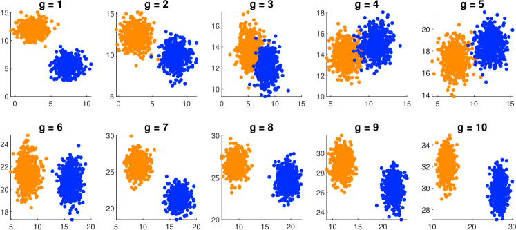
Figure 2: Synthetic samples in ten different intervals.

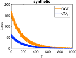
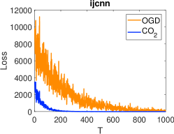
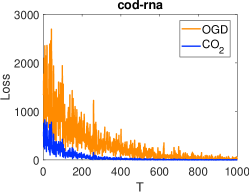
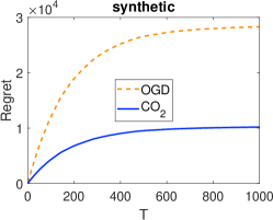
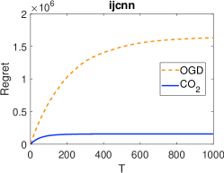
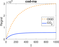
Figure 3: Regret and loss of CO₂ and OGD methods.

4 Empirical Analysis

In this section, we present empirical analysis to support our proposed theory and model.

4.1 Experimental Settings

We consider the problem of binary classification on multi-distributional data streams and compare the proposed CO₂ method with the OGD method on a synthetic dataset and two real-world datasets (i.e., ijcnn and cod-rna) from the LIBSVM repository Chang and Lin (2011). On the synthetic dataset, in each interval, independent and identically distributed samples in the same class are drawn from the same two-dimensional Gaussian distribution, and we randomly select two different means to construct two different Gaussian distributions with the same covariance $\mathbf{I}_{2}$ for generating samples with different ground truth labels. We slightly change the two means by adding different Gaussian noises for sampling in the next interval to model dynamic data streams. We construct $15$ intervals in our experiment, and the samples from the first $10$ intervals are presented in Fig. 2. We find that the data distributions change gradually, which matches the assumption of our dynamic setting. Similarly, for the two real-world datasets ijcnn and cod-rna, we randomly divide the entire dataset into $15$ intervals. After accessing all samples in one interval, we construct two different Gaussian distributions, and Gaussian noise is applied to the rest samples in other intervals, where the noise to samples in a class is drawn from the same distribution. Note that the two distributions for sampling noise should be reconstructed for each interval to ensure the data stream’s dynamic nature. For fair comparisons, we set the maximal number of maintained experts $K_{\text{max}}=5$ in CO₂ without loss of generality.

4.2 Experimental Results

Although the convergence rate for the generalization error of CO₂ is $O(1/\sqrt{T})$ which is consistent with the result of OGD in stationary and non-algorithmic cases, the theoretical analyses in Theorem 5 and Theorem 10 reveal that the proposed CO₂ method outperforms OGD on dynamic environments. To verify these two methods, we measure the regret $\sum_{t=1}^{T}f_{t}(\mathbf{w}_{t})-\sum_{t=1}^{T}f_{t}(\mathbf{w^{*}})$ and the loss of each sample $f_{T}(\mathbf{w}_{T})$ in the online interval, and the main results are summarized in Fig. 3. We observe that CO₂ has significantly lower loss than OGD at the early state, where only a few samples are received. The main reason is that CO₂ can apply offline expert knowledge to fill the gap of insufficient training samples. Also, the regret of CO₂ is small when $T$ is sufficiently large, and the regret gaps between CO₂ and OGD tend to be widened as $T$ increases. This is because CO₂ adapts to out-of-distribution samples in the online interval by adjusting the strategy of integrating the $K-1$ offline experts and the online expert after receiving the loss of each sample.

5 Conclusion

In this paper, we consider a more general and realistic scenario about nonstationary non-mixing multi-distributional data streams, in which several offline intervals with various distributions exist in addition to an out-of-distribution online interval. A novel online optimization method named Coupling Online-Offline learning (CO₂) is proposed to apply a meta-expert to adaptively couple the offline experts learned from the previous offline intervals and the online expert being trained on the fly in the online interval. We provide the theoretical guarantees about the CO₂ ways for knowledge transfer, the regret, and the generalization. To obtain a high-probability data-dependent bound on the generalization error of the output hypothesis from CO₂, we derive a specific excess risk bound by considering the loss function properties, the hypothesis class, the data distribution, and the regret of CO₂. Exploiting other assumptions and techniques to break through the bottlenecks in the generalization bound forms part of our future work.

6 Appendix - Supplementary Analysis

In this section, we present the proofs of all the theorems and lemmas. Our analysis follows some advanced techniques, including the self-bound property of smooth functions (Srebro et al., 2010), the analysis of adaptive online optimization method with multiple learning rates (van Erven and Koolen, 2016), the connection between agnostic PAC learning and online convex optimization (Hazan, 2016), empirical risk minimization for stochastic convex optimization (Zhang et al., 2017), and the bound of Rademacher complexity for any norm-regularized hypothesis class (Yousefi et al., 2018).

6.1 Proof of Lemma 3

According to the property of strong convexity (Shalev-Shwartz and Ben-David, 2014, Lemma 13.5.2), we know $L_{\mathcal{\widetilde{S}}}^{\gamma}(\mathbf{w})$ is $\gamma$-strongly convex since $L_{\mathcal{S}}(\mathbf{w})$ is convex and $\frac{\gamma}{2}\Omega(\mathbf{w})$ is $\gamma$-strongly convex. Accordingly, we have

$$\frac{\gamma}{2}\Omega\left(\mathbf{w}^{K}\right) \leq L_{\mathcal{\widetilde{S}}}\left(\sum_{k=1}^{K}\alpha_{B}^{k}\mathbf{w}_{B}^{k}\right)+\frac{\gamma}{2}\Omega\left(\sum_{k=1}^{K}\alpha_{B}^{k}\mathbf{w}^{k}_{B}\right)-L_{\mathcal{\widetilde{S}}}\left(\mathbf{w}^{K}\right)-\frac{\gamma}{2}\Omega\left(\mathbf{w}^{K}\right)$$

$$\leq\sum_{k=1}^{K}\alpha_{B}^{k}L_{\mathcal{\widetilde{S}}}\left(\mathbf{w}_{B}^{k}\right)+0-0-\frac{\gamma}{2}\Omega\left(\mathbf{w}^{K}\right).$$

Above, the first inequality is due to the strongly-convex property that $\frac{\gamma}{2}\|x-x^{*}\|_{2}^{2}\leq f(x)-f(x^{*})$ (Shalev-Shwartz and Ben-David, 2014, Lemma 13.5.3) and $\mathbf{w}^{K}$ is an empirical minimizer of $L_{\mathcal{\widetilde{S}}}^{\gamma}(\mathbf{w})$; the second inequality uses the condition that $L_{\mathcal{\widetilde{S}}}(\mathbf{w}^{K})\geq 0$ as assumed.

6.2 Proof of Theorem 4

By using the fact that $\mathbf{w}^{*}$ minimizes $L_{\mathcal{D}}(\mathbf{w})$ over the domain $\mathcal{W}$, we have

$$L_{\mathcal{D}}(\mathbf{w}^{*})-L_{\mathcal{D}}(\mathbf{w}^{K})\leq 0.$$ (10)

According to the property of strong convexity (Shalev-Shwartz and Ben-David, 2014, Lemma 13.5.2), $L_{\mathcal{D}}(\mathbf{w})+\frac{\gamma}{2}\Omega(\mathbf{w})$ is $\gamma$-strongly convex because the former term is convex and the last term is $\gamma$-strongly convex. Following the definition of strongly convex function, we have

$$\frac{\gamma}{2}\left\|\mathbf{w}^{K}-\mathbf{w}^{*}\right\|_{2}^{2}\leq L_{\mathcal{D}}(\mathbf{w}^{*})+\frac{\gamma}{2}\Omega(\mathbf{w}^{*})-L_{\mathcal{D}}(\mathbf{w}^{K})-\frac{\gamma}{2}\Omega(\mathbf{w}^{K})$$ (11)

$$+\left<\nabla L_{\mathcal{D}}(\mathbf{w}^{K})+\gamma\left(\mathbf{w}^{K}-\sum_{k=1}^{K}\alpha_{B}^{k}\mathbf{w}^{k}_{B}\right),\mathbf{w}^{K}-\mathbf{w}^{*}\right>.$$

To upper bound the last term above, we have

$$\left<\nabla L_{\mathcal{D}}\left(\mathbf{w}^{K}\right)+\gamma\left(\mathbf{w}^{K}-\sum_{k=1}^{K}\alpha_{B}^{k}\mathbf{w}^{k}_{B}\right),\mathbf{w}^{K}-\mathbf{w}^{*}\right>$$ (12)

$$\leq \left(\left\|\nabla L_{\mathcal{D}}(\mathbf{w}^{K})\right\|+\gamma\left\|\mathbf{w}^{K}-\sum_{k=1}^{K}\alpha_{B}^{k}\mathbf{w}^{k}_{B}\right\|\right)\left\|\mathbf{w}^{K}-\mathbf{w}^{*}\right\|$$

$$\leq \frac{4\left\|\nabla L_{\mathcal{D}}\left(\mathbf{w}^{K}\right)\right\|^{2}_{2}}{2\gamma}+\frac{\gamma\left\|\mathbf{w}^{K}-\mathbf{w}^{*}\right\|^{2}_{2}}{2\cdot 4}+\gamma\left(\frac{4\left\|\mathbf{w}^{K}-\sum_{k=1}^{K}\alpha_{B}^{k}\mathbf{w}^{k}_{B}\right\|_{2}^{2}}{2}+\frac{\left\|\mathbf{w}^{K}-\mathbf{w}^{*}\right\|^{2}_{2}}{2\cdot 4}\right)$$

where the first inequality uses the Cauchy-Schwarz inequality and the second inequality uses the Young’s inequality $\left<a,b\right>\leq\frac{1}{2}\|a\|_{2}^{2}+\frac{1}{2}\|b\|_{2}^{2}$.

Substituting Eqs. (10) and (LABEL:eq:hy2:3) into Eq. (11), we have

$$\left\|\mathbf{w}^{K}-\mathbf{w}^{*}\right\|^{2}_{2}\leq 2\Omega\left(\mathbf{w}^{*}\right)+\frac{8}{\gamma^{2}}\left\|\nabla L_{\mathcal{D}}\left(\mathbf{w}^{K}\right)\right\|^{2}_{2}+6\Omega\left(\mathbf{w}^{K}\right)$$

$$\leq 2\Omega\left(\mathbf{w}^{*}\right)+\frac{32L}{\gamma^{2}}+\frac{6\sum_{k=1}^{K}\alpha_{B}^{k}L_{\mathcal{\widetilde{S}}}\left(\mathbf{w}_{B}^{k}\right)}{\gamma}$$

where the second inequality is owing to Eq. (1) and Lemma 3.

6.3 Proof of Theorem 5

As shown in Eq. (8), the analysis is divided into two parts. First, we show the $\text{Regret}_{\text{ME}}$ of the meta-expert: the difference between the total cost it has incurred and that of the best existing expert of $K$ experts. Then, we demonstrate the $\text{Regret}_{\text{OE}}$ of the online expert: the difference between the total cost it has incurred and that of the empirical minimizer. Based on the pervious study (Cesa-Bianchi and Lugosi, 2006, Theorem 2.2), we define $W_{j}=\sum_{k=1}^{K}\alpha_{1}^{k}e^{-\nu\sum_{t=1}^{j}f_{t}(\mathbf{w}_{t}^{k})}$ and the lower bound of the related quantities is

$$\ln\frac{W_{T}}{W_{0}}= \ln\left(\frac{\sum_{k=1}^{K}\alpha_{1}^{k}e^{-\nu\sum_{t=1}^{T}f_{t}(\mathbf{w}_{t}^{k})}}{\sum_{k=1}^{K}\alpha_{1}^{k}}\right)$$ (13)

$$= \ln\left(\sum_{k=1}^{K}\alpha_{1}^{k}e^{-\nu\sum_{t=1}^{T}f_{t}(\mathbf{w}_{t}^{k})}\right)-\ln\left(\sum_{k=1}^{K}\alpha_{1}^{k}\right)$$

$$\geq \ln\max_{k\in[K]}\left(\alpha_{1}^{k}e^{-\nu\sum_{t=1}^{T}f_{t}(\mathbf{w}_{t}^{k})}\right)-\ln\left(\sum_{k=1}^{K}\alpha_{1}^{k}\right)$$

$$= -\nu\min_{k\in[K]}\left(\sum_{t=1}^{T}f_{t}(\mathbf{w}_{t}^{k})+\frac{1}{\nu}\ln\frac{1}{\alpha_{1}^{k}}\right)-\ln\left(\sum_{k=1}^{K}\alpha_{1}^{k}\right).$$

On the other hand, for $j\in[T]$ and $k\in[K]$, we can use the updating rule of $\alpha_{j}^{k}$ defined in Eq. (6) to obtain

$$\ln\frac{W_{j}}{W_{j-1}}= \log\left(\frac{\sum_{k=1}^{K}\alpha_{1}^{k}e^{-\nu\sum_{t=1}^{j}f_{t}(\mathbf{w}_{t}^{k})}}{\sum_{k=1}^{K}\alpha_{1}^{k}e^{-\nu\sum_{t=1}^{j-1}f_{t}(\mathbf{w}_{t}^{k})}}\right)$$ (14)

$$= \ln\left(\sum_{k=1}^{K}\frac{\alpha_{1}^{k}e^{-\nu\sum_{t=1}^{j-1}f_{t}(\mathbf{w}_{t}^{k})}}{\sum_{k=1}^{K}\alpha_{1}^{k}e^{-\nu\sum_{t=1}^{j-1}f_{t}(\mathbf{w}_{t}^{k})}}e^{-\nu f_{j}(\mathbf{w}_{j}^{k})}\right)$$

$$= \ln\left(\sum_{k=1}^{K}\alpha_{j}^{k}e^{-\nu f_{j}(\mathbf{w}_{j}^{k})}\right).$$

To bound the above result further, we require the following Hoeffding’s Lemma.

Lemma 11

(Cesa-Bianchi and Lugosi, 2006, Lemma 2.2) Let $X$ be a random variable with $a\leq X\leq b$, then for any $s\in\mathbb{R}$,

$$\ln E[e^{sX}]\leq sE[X]+\frac{s^{2}(b-a)^{2}}{8}.$$

Recalling Assumption 4 that $0\leq f_{t}(\cdot)\leq 1$ and combining that with Lemma 11, we have

$$\ln\left(\sum_{k=1}^{K}\alpha_{j}^{k}e^{-\nu f_{j}(\mathbf{w}_{j}^{k})}\right)\leq-\nu\sum_{k=1}^{K}\alpha_{t}^{k}f_{t}(\mathbf{w}_{t}^{k})+\frac{\nu^{2}\left(1-0\right)^{2}}{8}\leq-\nu f_{t}(\mathbf{w}_{t})+\frac{\nu^{2}}{8}$$ (15)

where the last inequality is owing to the Jensen’s inequality.

Substituting Eqs. (15) into (14) and accumulating the result from $t=1$ to $t=T$, we have

$$\sum_{j=1}^{T}\ln\frac{W_{j}}{W_{j-1}}=\ln\frac{W_{T}}{W_{0}}=-\nu\sum_{t=1}^{T}f_{t}(\mathbf{w}_{t})+\frac{T\nu^{2}}{8}.$$ (16)

By combining Eq. (13) with Eq. (16), we have

$$\sum_{t=1}^{T}f_{t}(\mathbf{w}_{t})-\min_{k\in[K]}\left(\sum_{t=1}^{T}f_{t}(\mathbf{w}_{t}^{k})+\frac{1}{\nu}\ln\frac{1}{\alpha_{1}^{k}}\right)\leq\frac{T\nu}{8}+\ln\left(\sum_{k=1}^{K}\alpha_{1}^{k}\right)$$

which implies

$$\sum_{t=1}^{T}f_{t}(\mathbf{w}_{t})-\min_{k\in[K]}\sum_{t=1}^{T}f_{t}(\mathbf{w}_{t}^{k})\leq\frac{T\nu}{8}+\ln\left(\sum_{k=1}^{K}\alpha_{1}^{k}\right)+\max_{k\in[K]}\frac{1}{\nu}\ln\frac{1}{\alpha_{1}^{k}}.$$ (17)

With Eq. (5), we have

$$\sum_{k=1}^{K}\alpha_{1}^{k}=\frac{K+1}{K}\left[\left(\frac{1}{K}-\frac{1}{K+1}\right)+,\ldots,+\left(\frac{1}{1}-\frac{1}{2}\right)\right]=\frac{K+1}{K}\cdot\frac{K}{K+1}=1,$$ (18)

and for any $2\leq k\leq K$, we have

$$\frac{K}{K+1}\left(\alpha_{1}^{k-1}-\alpha_{1}^{k}\right)\geq(\frac{1}{K-k}-\frac{1}{K+1-k})-(\frac{1}{K+1-k}-\frac{1}{K+2-k})\geq 0,$$

so $\{\alpha_{1}^{k}\}$ is in the ascending order and

$$\max_{k\in[K]}\ln\frac{1}{\alpha_{1}^{k}}=\ln\frac{1}{\alpha_{1}^{1}}=2\ln K.$$ (19)

Substitute Eqs. (18) and (19) into Eq. (17), we have

$$\frac{T\nu}{8}+\frac{2}{\nu}\ln K,$$ (20)

and minimize this function toward $\nu$ to obtain

$$\nu=4\sqrt{\frac{\ln K}{T}}.$$ (21)

Substitute Eqs. (5) and (21) into Eq. (20), we have

$$\text{Regret}_{\text{ME}}\leq\sqrt{T\ln K}.$$ (22)

We apply the standard OSG to optimize the online expert $\mathbf{w}^{K}_{t}$. Following the previous result (Hazan, 2016, Theorem 3.1), setting the step size $\eta_{t}=\frac{D}{\sqrt{\beta t}}$, we have

$$\text{Regret}_{\text{OE}}\leq 6D\sqrt{T\beta}.$$ (23)

We obtain $\text{Regret}_{\text{CO${}_{2}$}}$ by combining Eq. (22) with Eq. (23). According to Eq. (8) and the requirement that CO₂ should surpass its online expert, we obtain the upper bound of $K$ by solving the following inequality

$$\sqrt{T\ln K}+\text{Regret}_{\text{KE}}\leq 6D\sqrt{T\beta}.$$

6.4 Proof of Lemma 6

To proceed, we introduce the following norm concentration inequality.

Lemma 12

(Smale and Zhou, 2009, Proposition 1) Let $\xi$ be a random variable on $(Z,\rho)$ with values in a Hilbert space and be randomly drawn according to $\rho$ satisfying $\|\xi\|\leq M\leq\infty$. Then, for any $0<\delta<1$, with a probability at least $1-\delta$,

$$\left\|\frac{1}{m}\sum_{i=1}^{m}\left(\xi_{i}-\mathbb{E}[\xi_{i}]\right)\right\|\leq\frac{4M}{\sqrt{m}}\log\frac{2}{\delta}.$$

Using Lemma 12 with the results $\|\frac{1}{T}\sum_{t=1}^{T}f_{t}(\mathbf{w}_{t})\|\leq 1$ and $\|\frac{1}{T}\sum_{t=1}^{T}f_{t}(\mathbf{w}^{*})\|\leq 1$ implied from Assumption 4, with probability at least $1-\delta$, we have

$$\frac{1}{T}\sum_{t=1}^{T}L_{\mathcal{D}}(\mathbf{w}_{t}) \leq\frac{1}{T}\sum_{t=1}^{T}f_{t}(\mathbf{w}_{t})+\frac{4\log(2/\delta)}{\sqrt{T}}$$ (24)

$$\frac{1}{T}\sum_{t=1}^{T}f_{t}(\widehat{\mathbf{w}}) \leq\frac{1}{T}\sum_{t=1}^{T}L_{\mathcal{D}}(\widehat{\mathbf{w}})+\frac{4\log(2/\delta)}{\sqrt{T}}.$$

Putting the two results in Eq. (24) together, with probability at least $1-\delta$, we have

$$\frac{1}{T}\sum_{t=1}^{T}L_{\mathcal{D}}(\mathbf{w}_{t})-L_{\mathcal{D}}(\widehat{\mathbf{w}})\leq \frac{1}{T}\left(\sum_{t=1}^{T}f_{t}(\mathbf{w}_{t})-\sum_{t=1}^{T}f_{t}(\widehat{\mathbf{w}})\right)+\frac{4\log(4/\delta)}{\sqrt{T}}$$ (25)

$$\leq \frac{\sqrt{\ln K}+6D\sqrt{\beta}}{\sqrt{T}}+\frac{4\log(4/\delta)}{\sqrt{T}}$$

where the first inequality is owing to the Hoeffding’s inequality (Boucheron et al., 2013, Theorem 2.8) and the second inequality follows Theorem 5.

6.5 Proof of Lemma 7

Our analysis is based on the techniques used in (Zhang et al., 2017). For simplicity, we assume $\dot{b}_{t}=\nabla f_{t}(\mathbf{w}^{*})$ and $\ddot{b}_{t}=\nabla f_{t}(\widehat{\mathbf{w}})-\nabla f_{t}(\mathbf{w}^{*})$, so we know

$$\nabla L_{\mathcal{S}}(\mathbf{w}^{*})=\frac{1}{T}\sum_{t=1}^{T}\dot{b}_{t}$$ (26)

$$\nabla L_{\mathcal{D}}(\mathbf{w}^{*})=\mathbb{E}[\dot{b}]$$

$$\nabla L_{\mathcal{S}}(\widehat{\mathbf{w}})-\nabla L_{\mathcal{S}}(\mathbf{w}^{*})=\frac{1}{T}\sum_{t=1}^{T}\ddot{b}_{t}$$

$$\nabla L_{\mathcal{D}}(\widehat{\mathbf{w}})-\nabla L_{\mathcal{D}}(\mathbf{w}^{*})=\mathbb{E}[\ddot{b}].$$

By the Karush-Kuhn-Tucker (KKT) (Hazan, 2016, Theorem 2.2) condition for convex function $L_{\mathcal{S}}(\cdot)$ and $L_{\mathcal{D}}(\cdot)$, we have

$$\left<\nabla L_{\mathcal{S}}(\widehat{\mathbf{w}}),\mathbf{w}-\widehat{\mathbf{w}}\right>\geq 0,$$ (27)

$$\left<\nabla L_{\mathcal{D}}(\mathbf{w}^{*}),\mathbf{w}-\mathbf{w}^{*}\right>\geq 0,\forall\mathbf{w}\in\mathcal{W}.$$

We first upper bound the excess risk $L_{\mathcal{D}}(\widehat{\mathbf{w}})-L_{\mathcal{D}}(\mathbf{w}^{*})$ by two terms with the same form and then further derive the upper bounds of the two terms by similar methods.

$$L_{\mathcal{D}}(\widehat{\mathbf{w}})-L_{\mathcal{D}}(\mathbf{w}^{*})\leq \left<\nabla L_{\mathcal{D}}(\widehat{\mathbf{w}}),\widehat{\mathbf{w}}-\mathbf{w}^{*}\right>$$ (28)

$$= \left<\mathbb{E}[\ddot{b}]+\mathbb{E}[\dot{b}],\widehat{\mathbf{w}}-\mathbf{w}^{*}\right>$$

$$= \left<\mathbb{E}[\ddot{b}]-\frac{1}{T}\sum_{t=1}^{T}\ddot{b}_{t}+\mathbb{E}[\dot{b}]+\frac{1}{T}\sum_{t=1}^{T}\ddot{b}_{t},\widehat{\mathbf{w}}-\mathbf{w}^{*}\right>$$

$$\leq \left<\mathbb{E}[\ddot{b}]-\frac{1}{T}\sum_{t=1}^{T}\ddot{b}_{t}+\mathbb{E}[\dot{b}]+\frac{1}{T}\sum_{t=1}^{T}\dot{b}_{t},\widehat{\mathbf{w}}-\mathbf{w}^{*}\right>$$

$$\leq \underbrace{\left\|\mathbb{E}[\ddot{b}]-\frac{1}{T}\sum_{t=1}^{T}\ddot{b}_{t}\right\|\left\|\widehat{\mathbf{w}}-\mathbf{w}^{*}\right\|}_{:=B_{1}}+\underbrace{\left\|\mathbb{E}[\dot{b}]-\frac{1}{T}\sum_{t=1}^{T}\dot{b}_{t}\right\|\left\|\widehat{\mathbf{w}}-\mathbf{w}^{*}\right\|}_{:B_{2}}.$$

In the above, the first inequality is owing to the convexity of $L_{\mathcal{D}}(\cdot)$ over the domain $\mathcal{W}$, the second inequality applies Eq. (28) for convex function $L_{\mathcal{S}}(\cdot)$ with respect to $\mathbf{w}^{*}$: $\left<\nabla L_{\mathcal{S}}(\widehat{\mathbf{w}}),\widehat{\mathbf{w}}-\mathbf{w}^{*}\right>\leq 0$ and uses $\mathbb{E}[\dot{b}]+\nabla L_{\mathcal{S}}(\widehat{\mathbf{w}})-\frac{1}{T}\sum_{t=1}^{T}\dot{b}_{t}$; the third inequality uses the Cauchy-Schwarz inequality.

Note that $B_{1}$ and $B_{2}$ have the same structure. To bound the variance terms in $B_{1}$ and $B_{2}$, we introduce the following norm concentration inequality in a Hilbert space.

Lemma 13

(Steve and Zhou, 2007, Lemma 2) Let $\xi$ be a random variable on $(Z,\rho)$ with values in a Hilbert space, assume $\|\xi\|\leq M\leq\infty$ almost surely holds, denote $\sigma^{2}(\xi)=\mathbb{E}(\|\xi\|^{2})$, and let ${\xi_{i}}_{i=1}^{m}$ be independent random drawers of $\rho$, for any $0\leq\delta\leq 1$, with confidence $1-\delta$,

$$\left\|\frac{1}{m}\sum_{i=1}^{m}\left(\xi_{i}-\mathbb{E}[\xi_{i}]\right)\right\|\leq\frac{2M\log(2/\delta)}{m}+\sqrt{\frac{2\sigma^{2}(\xi)\log(2/\delta)}{m}}.$$

To use this lemma to upper bound $B_{1}$ and $B_{2}$, we need the bounds for $\|\dot{b}_{t}\|$, $\mathbb{E}\|\dot{b}\|^{2}_{2}$, $\|\ddot{b}_{t}\|$, $\mathbb{E}\|\ddot{b}\|^{2}_{2}$. From Eq. (1), we have

$$\|\dot{b}_{t}\|\leq 2\sqrt{\beta},\mathbb{E}\|\dot{b}\|^{2}_{2}\leq 4\beta.$$ (29)

With Assumption 5, we have

$$\|\ddot{b}_{t}\|\leq\beta\|\widehat{\mathbf{w}}-\mathbf{w}^{*}\|.$$

Based on that, by using the properties of smooth function (Nesterov, 2004, Theorem 2.1.5), we have

$$\|\ddot{b}_{t}\|_{2}^{2}\leq 2\beta\left(f_{t}(\widehat{\mathbf{w}})-f_{t}(\mathbf{w}^{*})-\left<\nabla f_{t}(\widehat{\mathbf{w}}),\widehat{\mathbf{w}}-\mathbf{w}^{*}\right>\right).$$ (30)

Taking the expectation on both sides, we have

$$\mathbb{E}\|\ddot{b}\|_{2}^{2} \leq 2\beta\left(L_{\mathcal{D}}(\widehat{\mathbf{w}})-L_{\mathcal{D}}(\mathbf{w}^{*})-\left<\nabla L_{\mathcal{D}}(\widehat{\mathbf{w}}),\widehat{\mathbf{w}}-\mathbf{w}^{*}\right>\right)\leq 2\beta\left(L_{\mathcal{D}}(\widehat{\mathbf{w}})-L_{\mathcal{D}}(\mathbf{w}^{*})\right),$$ (31)

where the last inequality applies Eq. (28) to the convex function $L_{\mathcal{D}}(\cdot)$ with respect to $\widehat{\mathbf{w}}$.

Based on Lemma 13, we establish the uniform convergence of $\frac{1}{T}\sum_{t=1}^{T}\dot{b}_{t}$ to $\mathbb{E}[\dot{b}]$ and $\frac{1}{T}\sum_{t=1}^{T}\ddot{b}_{t}$ to $\mathbb{E}[\ddot{b}]$. By using Eqs. (30) and (31) with Lemma 13, with probability at least $1-\delta$, we have

$$B_{1}\leq \frac{2\beta\|\widehat{\mathbf{w}}-\mathbf{w}^{*}\|_{2}^{2}\log(2/\delta)}{T}+2\|\widehat{\mathbf{w}}-\mathbf{w}^{*}\|\sqrt{\frac{\beta L_{\mathcal{D}}(\widehat{\mathbf{w}})-L_{\mathcal{D}}(\mathbf{w}^{*})\log(2/\delta)}{T}}$$ (32)

$$\leq \frac{3\beta\|\widehat{\mathbf{w}}-\mathbf{w}^{*}\|_{2}^{2}\log(2/\delta)}{T}+\frac{L_{\mathcal{D}}(\widehat{\mathbf{w}})-L_{\mathcal{D}}(\mathbf{w}^{*})}{2}$$

$$\leq \frac{12\beta R^{2}\log(2/\delta)}{T}+\frac{L_{\mathcal{D}}(\widehat{\mathbf{w}})-L_{\mathcal{D}}(\mathbf{w}^{*})}{2},$$

where the second inequality uses the Young’s inequality and the third inequality is owing to that Assumption 3 implies $\|\widehat{\mathbf{w}}-\mathbf{w}^{*}\|\leq 2R$. By using the same method as above with Eq. (29), with probability at least $1-\delta$, we have

$$B_{2}\leq\frac{4R\sqrt{\beta}\log(2/\delta)}{T}+4R\sqrt{\frac{2\beta\log(2/\delta)}{T}}.$$ (33)

We complete the proof by substituting Eqs. (32) and (33) into Eq. (28).

6.6 Proof of Lemma 8

By using the definition of the Rademacher complexity (Bartlett and Mendelson, 2002), we have

$$\mathcal{R}_{\mathcal{D}}(\mathcal{W})=\mathbb{E}_{\mathbf{S},\mathbf{\sigma}}\left[\sup_{\mathbf{w}\in\mathcal{W}}\frac{1}{T}\sum_{t=1}^{T}\sigma_{t}\left<\mathbf{w},\mathbf{x}_{t}\right>\right].$$

Let $\Gamma_{i}=\left<\sum_{t=1}^{T}\sigma_{t}\mathbf{x}_{t},\mathbf{u}_{i}\right>/T$ for any $i\geq 1$ and $\theta\geq i$, by using advanced techniques of the Rademacher complexities (Yousefi et al., 2018), we have

$$\mathbb{E}_{\mathbf{S},\mathbf{\sigma}}\left[\sup_{\mathbf{w}\in\mathcal{W}}\sigma_{t}\left<\mathbf{w},\frac{1}{T}\sum_{t=1}^{T}\mathbf{x}_{t}\right>\right]$$

$$= \mathbb{E}_{\mathbf{S},\mathbf{\sigma}}\left[\sup_{\mathbf{w}\in\mathcal{W}}\sigma_{t}\left<\mathbf{w},\sum_{i=1}^{\infty}\left<\frac{1}{T}\sum_{t=1}^{T}\mathbf{x}_{t},\mathbf{u}_{i}\right>\mathbf{u}_{i}\right>\right]$$

$$\leq \mathbb{E}_{\mathbf{S},\mathbf{\sigma}}\left[\sup_{\mathbf{w}\in\mathcal{W}}\left<\mathbf{w},\sum_{i=1}^{\theta}\Gamma_{i}\mathbf{u}_{i}\right>\right]+\mathbb{E}_{\mathbf{S},\mathbf{\sigma}}\left[\sup_{\mathbf{w}\in\mathcal{W}}\left<\mathbf{w},\sum_{i=\theta+1}^{\infty}\Gamma_{i}\mathbf{u}_{i}\right>\right]$$

The above inequality is owing to the Jensen’s inequality. Based on the Cauchy-Schwarz inequality, we have the following upper bounds for the last two terms

$$\mathbb{E}_{\mathbf{S},\mathbf{\sigma}}\left[\sup_{\mathbf{w}\in\mathcal{W}}\left<\mathbf{w},\sum_{i=1}^{\theta}\Gamma_{i}\mathbf{u}_{i}\right>\right]= \mathbb{E}_{\mathbf{S},\mathbf{\sigma}}\left[\sup_{\mathbf{w}\in\mathcal{W}}\left<\sum_{i=1}^{\theta}\sqrt{\lambda_{i}}\left<\mathbf{w},\mathbf{u}_{i}\right>\mathbf{u}_{i},\sum_{i=1}^{\theta}\frac{1}{\sqrt{\lambda_{i}}}\Gamma_{i}\mathbf{u}_{i}\right>\right]$$

$$\leq \mathbb{E}_{\mathbf{S},\mathbf{\sigma}}\left[\sup_{\mathbf{w}\in\mathcal{W}}\left\|\sum_{i=1}^{\theta}\sqrt{\lambda_{i}}\left<\mathbf{w},\mathbf{u}_{i}\right>\mathbf{u}_{i}\right\|_{2}\left\|\sum_{i=1}^{\theta}\frac{1}{\sqrt{\lambda_{i}}}\Gamma_{i}\mathbf{u}_{i}\right\|_{2}\right]$$

$$= \underbrace{\sup_{\mathbf{w}\in\mathcal{W}}\sqrt{\sum_{i=1}^{\theta}\lambda_{i}\left<\mathbf{w},\mathbf{u}_{i}\right>^{2}}}_{:=U_{1}}\underbrace{\mathbb{E}_{\mathbf{S},\mathbf{\sigma}}\sqrt{\sum_{i=1}^{\theta}\frac{1}{\lambda_{i}}\Gamma_{i}^{2}}}_{:=U_{2}},$$

and

$$\mathbb{E}_{\mathbf{S},\mathbf{\sigma}}\left[\sup_{\mathbf{w}\in\mathcal{W}}\left<\mathbf{w},\sum_{i=\theta+1}^{\infty}\Gamma_{i}\mathbf{u}_{i}\right>\right]\leq\underbrace{\sup_{\mathbf{w}\in\mathcal{W}}\left\|\mathbf{w}\right\|\mathbb{E}_{\mathbf{S},\mathbf{\sigma}}\left[\left\|\sum_{i=\theta+1}^{\infty}\Gamma_{i}\mathbf{u}_{i}\right\|\right]}_{:=U_{3}}.$$

6.6.1 Bounding $U_{1}$:

Enlarging $U_{1}$ by replacing $\theta$ with $\infty$, we have the following upper bound

$$U_{1}\leq\sup_{\mathbf{w}\in\mathcal{W}}\sqrt{\sum_{i=1}^{\infty}\lambda_{i}\left<\mathbf{w},\mathbf{u}_{i}\right>\left<\mathbf{w},\mathbf{u}_{i}\right>}=\sup_{\mathbf{w}\in\mathcal{W}}\sqrt{\mathbb{E}\left<\mathbf{w}\mathbf{w}^{T},[\mathbf{x}\mathbf{x}^{T}]\right>}\leq DR,$$

where the last inequality uses Assumptions 3 and  2.

6.6.2 Bounding $U_{2}$:

By using the Jensen’s inequality, we have

$$U_{2}\leq \sqrt{\sum_{i=1}^{\theta}\mathbb{E}_{\mathbf{S},\mathbf{\sigma}}\frac{1}{\lambda_{i}}\left<\frac{1}{T}\sum_{t=1}^{T}\sigma_{t}\mathbf{x}_{t},\mathbf{u}_{i}\right>^{2}}$$

$$= \sqrt{\sum_{i=1}^{\theta}\mathbb{E}_{\mathbf{S},\mathbf{\sigma}}\frac{1}{\lambda_{i}T^{2}}\sum_{t=1}^{T}\sum_{t^{\prime}=1}^{T}\sigma_{t}\sigma_{t}^{\prime}\left<\mathbf{x}_{t},\mathbf{u}_{i}\right>\left<\mathbf{x}_{t}^{\prime},\mathbf{u}_{i}\right>}$$

$$= \sqrt{\sum_{i=1}^{\theta}\frac{1}{\lambda_{i}T}\left<\frac{1}{T}\sum_{t=1}^{T}\mathbb{E}_{\mathbf{S}}\left[\mathbf{x}_{t}\mathbf{x}_{t}^{T}\right],\mathbf{u}_{i}\mathbf{u}_{i}^{T}\right>}$$

$$= \sqrt{\sum_{i=1}^{\theta}\frac{1}{\lambda_{i}T}\left<\sum_{j=1}^{\infty}\lambda_{j}\mathbf{u}_{j}\mathbf{u}_{j}^{T},\mathbf{u}_{i}\mathbf{u}_{i}^{T}\right>}$$

$$= \sqrt{\sum_{i=1}^{\theta}\frac{1}{\lambda_{i}T}\lambda_{i}}=\sqrt{\frac{\theta}{T}}.$$

6.6.3 Bounding $U_{3}$:

Recall the definition of $\Gamma_{i}$, we have

$$U_{3}\leq R\mathbb{E}_{\mathbf{S},\mathbf{\sigma}}\sqrt{\left\|\sum_{i=\theta+1}^{\infty}\left<\frac{1}{T}\sum_{t=1}^{T}\sigma_{t}\mathbf{x}_{t},\mathbf{u}_{i}\right>\mathbf{u}_{i}\right\|^{2}_{2}},$$ (34)

where the inequality is owing to our assumption $\sup_{\mathbf{w}\in\mathcal{W}}\left\|\mathbf{w}\right\|\leq R$. To derive its bound further, we introduce the Khintchine-Kahane inequality.

Lemma 14

(Hoffmann-Jorgensen et al., 2012) Let $\mathcal{H}$ be an inner-product space with the induced norm $\|\cdot\|_{\mathcal{H}}$, $v_{1},\ldots,v_{n}\in\mathcal{H}$ and $\sigma_{1},\ldots,\sigma_{n}$ i.i.d. Rademacher random variables. Then, for any $p\geq 1$, we have

$$\mathbb{E}\|\sum_{i=1}^{n}\sigma_{i}v_{i}\|_{\mathcal{H}}^{p}\leq\left(c\sum_{i=1}^{n}\|v_{i}\|_{\mathcal{H}}^{2}\right)^{\frac{p}{2}}$$

where $c:=\max{1,p-1}$. The inequality also holds for $p$ in place of $c$.

With Lemma 14, we have

$$\mathbb{E}_{\mathbf{S},\mathbf{\sigma}}\sqrt{\left\|\sum_{i=\theta+1}^{\infty}\left<\frac{1}{T}\sum_{t=1}^{T}\sigma_{t}\mathbf{x}_{t},\mathbf{u}_{i}\right>\mathbf{u}_{i}\right\|^{2}_{2}}\leq \frac{1}{\sqrt{T}}\mathbb{E}_{\mathbf{S}}\sqrt{\frac{1}{T}\sum_{t=1}^{T}\left\|\sum_{i=\theta+1}^{\infty}\left<\mathbf{x}_{t},\mathbf{u}_{i}\right>\mathbf{u}_{i}\right\|^{2}_{2}}$$ (35)

$$= \frac{1}{\sqrt{T}}\mathbb{E}_{\mathbf{S}}\sqrt{\frac{1}{T}\sum_{t=1}^{T}\sum_{i=\theta+1}^{\infty}\left<\mathbf{x}_{t},\mathbf{u}_{i}\right>^{2}}.$$

Although we can bound Eq. (35) further according to the following result obtained from Assumption 2

$$\sum_{i=\theta+1}^{\infty}\left<\mathbf{x}_{t},\mathbf{u}_{i}\right>^{2}=\left<\sum_{i=\theta+1}^{\infty}\left<\mathbf{x}_{t},\mathbf{u}_{i}\right>\mathbf{u}_{i},\mathbf{x}_{t}\right>\leq\left<\mathbf{x}_{i},\mathbf{x}_{i}\right>=D^{2},$$ (36)

we pursue a tighter bound by introducing the Rosenthal-Young inequality.

Lemma 15

(Kloft and Blanchard, 2012, Lemma 3) Let the independent nonnegative random variables $X_{1},\ldots,X_{n}$ satisfy $X_{i}\leq B\leq+\infty$ almost surely for all $i=1,\ldots,n$, if $q\geq\frac{1}{2}$, $c_{q}:=(2qe)^{q}$, then the following holds

$$\mathbb{E}\left(\frac{1}{n}\sum_{i=1}^{n}X_{i}\right)^{q}\leq c_{q}\left[\left(\frac{B}{n}\right)^{q}+\left(\frac{1}{n}\sum_{i=1}^{n}\mathbb{E}X_{i}\right)^{q}\right].$$

By combining Eq. (36) with Lemma 15, we have

$$\mathbb{E}_{\mathbf{S}}\sqrt{\frac{1}{T}\sum_{t=1}^{T}\sum_{i=\theta+1}^{\infty}\left<\mathbf{x}_{t},\mathbf{u}_{i}\right>^{2}}\leq \sqrt{e}\left(\frac{D}{\sqrt{T}}+\sqrt{\frac{1}{T}\sum_{i=\theta+1}^{\infty}\sum_{t=1}^{T}\mathbb{E}_{\mathbf{S}}\left<\mathbf{x}_{t},\mathbf{u}_{i}\right>^{2}}\right)$$ (37)

$$= D\sqrt{\frac{e}{T}}+\sqrt{\frac{e}{T}\sum_{i=\theta+1}^{\infty}\lambda_{i}}.$$

To obtain the upper bound of $U_{3}$, we combine Eqs. (34), (35) and (37).

To sum up, we can complete the proof by

$$\mathcal{R}_{\mathcal{D}}(\mathcal{W})= U_{1}\cdot U_{2}+U_{3}$$

$$\leq DR\sqrt{\frac{\theta}{T}}+\frac{R}{T}\sqrt{e\sum_{i=\theta+1}^{\infty}\lambda_{i}}+\frac{DR\sqrt{e}}{T}$$

$$\leq R\sqrt{\frac{1}{T}\left(D^{2}\theta+\sum_{i=\theta+1}^{\infty}\frac{e\lambda_{i}}{T}\right)}+\frac{DR\sqrt{e}}{T}$$

$$= R\sqrt{\frac{1}{T}\left(\sum_{i=1}^{\theta}D^{2}+\sum_{i=\theta+1}^{\infty}\frac{e\lambda_{i}}{T}\right)}+\frac{DR\sqrt{e}}{T}.$$

In the above, the first inequality uses the bounds of $U_{1}$, $U_{2}$ and $U_{3}$ we obtained, the second inequality is owing to the inequality of arithmetic and geometric means for nonnegative numbers: $2\sqrt{xy}\leq x+y\Leftrightarrow\sqrt{x}+\sqrt{y}\leq\sqrt{2x+2y}$. Note that the above bound for $\mathcal{R}_{\mathcal{D}}(\mathcal{W})$ holds for any positive integer $\theta\geq 1$, we obtain the tightest result by minimizing the upper bound, that is

$$\mathcal{R}_{\mathcal{D}}(\mathcal{W})\leq R\sqrt{\frac{1}{T}\min_{\theta\in\mathbb{N}}\left(\sum_{i=1}^{\theta}D^{2}+\sum_{i=\theta+1}^{\infty}\frac{e\lambda_{i}}{T}\right)}+\frac{DR\sqrt{e}}{T}$$

$$= R\sqrt{\frac{1}{T}\sum_{i=1}^{\infty}\left(D^{2}\wedge\frac{e\lambda_{i}}{T}\right)}+\frac{DR\sqrt{e}}{T},$$

where the equality is owing to that the sequence of eigenvalues $\{\lambda_{i}\}$ is in the ascending order.

6.7 Proof of Lemma 9

Based on the divide-and-conquer idea, we split our target into three more comfortable summands and derive their bounds respectively,

$$L_{\mathcal{D}}(\widehat{\mathbf{w}})-L_{\mathcal{D}}(\mathbf{w}^{*})=\left(L_{\mathcal{D}}(\widehat{\mathbf{w}})-L_{\mathcal{S}}(\widehat{\mathbf{w}})\right)+\left(L_{\mathcal{S}}(\widehat{\mathbf{w}})-L_{\mathcal{S}}(\mathbf{w}^{*})\right)+\left(L_{\mathcal{S}}(\mathbf{w}^{*})-L_{\mathcal{D}}(\mathbf{w}^{*})\right).$$ (38)

Recall that $l$ is a nonnegative function. To bound the generation error $L_{\mathcal{D}}(\widehat{\mathbf{w}})-L_{\mathcal{S}}(\widehat{\mathbf{w}})$ by the Rademacher complexity for this nonnegative function, we need the following two lemmas.

Lemma 16

(Shalev-Shwartz and Ben-David, 2014, Theorem 26.5) Assume that the loss function $l(h,z)$ is bounded by $b$ for all $z$ and $h\in\mathcal{H}$, $S$ is a $m$-samples data set. With probability of at least $1-\delta$, for all $h\in\mathcal{H}$,

$$L_{\mathcal{D}}(h)-L_{\mathcal{S}}(h)\leq 2\mathcal{R}(l\circ\mathcal{H})+b\sqrt{\frac{2\ln(2/\delta)}{m}}.$$

Lemma 17

(Srebro et al., 2010, Lemma 2.2) For a nonnegative $\beta$-smooth loss $l$ bounded by $b$ and any function class $\mathcal{H}$, the Rademacher Complexity on a $m$-sample data set is

$$\mathcal{R}(l\circ\mathcal{H})\leq 21\sqrt{6\beta b}\log^{\frac{3}{2}}(64m)\mathcal{R}(\mathcal{H}).$$

With Assumption 4, we know $|l(\left<\mathbf{w},\mathbf{x}\right>,y)|\leq 1$. By combing Lemmas 16 and  17 under the condition that $\widehat{\mathbf{w}}\in\mathcal{W}$, with probability at least $1-\delta$, we have

$$L_{\mathcal{D}}(\widehat{\mathbf{w}})-L_{\mathcal{S}}(\widehat{\mathbf{w}})\leq 2\mathcal{R}_{\mathcal{D}}(l\circ\mathcal{W})+\sqrt{\frac{2\log(2/\delta)}{T}}$$ (39)

$$\leq 42\sqrt{6\beta}\log^{\frac{3}{2}}(64T)\mathcal{R}_{\mathcal{D}}(\mathcal{W})+\sqrt{\frac{2\log(2/\delta)}{T}}.$$

Note that the above result ignores the specificity of $\widehat{\mathbf{w}}$. We utilize the specificity of $\widehat{\mathbf{w}}$ as well as $\mathbf{w}^{*}$ to bound the next two summands.

Recall that $\widehat{\mathbf{w}}$ is an empirical minimizer of $L_{\mathcal{S}}(\mathbf{w})$ over the domain $\mathcal{W}$, we have

$$L_{\mathcal{S}}(\widehat{\mathbf{w}})-L_{\mathcal{S}}(\mathbf{w}^{*})\leq 0.$$ (40)

Because $\mathbf{w}^{*}$ is independent of the data set $\mathcal{S}$ and $f_{1}(\mathbf{w}^{*}),\ldots,f_{T}(\mathbf{w}^{*})$ is a sequence of i.i.d. random variables, we have $\mathbb{E}_{\mathcal{S}^{\prime}}[L_{\mathcal{S}^{\prime}}(\mathbf{w}^{*})]=L_{\mathcal{D}}(\mathbf{w}^{*})$. With Assumption 4, we know that $\mathbb{P}[0\leq f_{t}(\mathbf{w}^{*})\leq 1]=1$ for every $t\in[T]$. The Hoeffding’s inequality (Boucheron et al., 2013, Theorem 2.8) implies that with probability at least $1-\delta$, we have

$$L_{\mathcal{S}}(\mathbf{w}^{*})-L_{\mathcal{D}}(\mathbf{w}^{*})\leq\sqrt{\frac{\log(2/\delta)}{2T}}.$$ (41)

We complete the proof by substituting Eqs. (40), (41) and (39) into Eq. (38).

References

Adams and Nobel (2010)
Terrence M. Adams and Andrew B. Nobel.
Uniform convergence of vapnik-chervonenkis classes under ergodic
sampling.
The Annals of Probability, 38(4):1345–1367, 2010.
Agarwal and Duchi (2013)
Alekh Agarwal and John C. Duchi.
The generalization ability of online algorithms for dependent data.
IEEE Trans. Information Theory, 59(1):573–587, 2013.
Bartlett and Mendelson (2002)
Peter L. Bartlett and Shahar Mendelson.
Rademacher and gaussian complexities: Risk bounds and structural
results.
J. Mach. Learn. Res., 3:463–482, 2002.
Besbes et al. (2015)
Omar Besbes, Yonatan Gur, and Assaf J. Zeevi.
Non-stationary stochastic optimization.
Operations Research, 63(5):1227–1244,
2015.
Boucheron et al. (2013)
Stéphane Boucheron, Gábor Lugosi, and Pascal Massart.
Concentration Inequalities - A Nonasymptotic Theory of
Independence.
Oxford university press, 2013.
Bubeck et al. (2013)
Sébastien Bubeck, Nicolò Cesa-Bianchi, and Gábor Lugosi.
Bandits with heavy tail.
IEEE Trans. Information Theory, 59(11):7711–7717, 2013.
Buchbinder et al. (2016)
Niv Buchbinder, Shahar Chen, Joseph Naor, and Ohad Shamir.
Unified algorithms for online learning and competitive analysis.
Math. Oper. Res., 41(2):612–625, 2016.