Physics-Guided Problem Decomposition for Scaling
Deep Learning of High-dimensional Eigen-Solvers:
The Case of Schrödinger’s Equation

Abstract.

Given their ability to effectively learn non-linear mappings and perform fast inference, deep neural networks (NNs) have been proposed as a viable alternative to traditional simulation-driven approaches for solving high-dimensional eigenvalue equations (HDEs), which are the foundation for many scientific applications. Unfortunately, for the learned models in these scientific applications to achieve generalization, a large, diverse, and preferably annotated dataset is typically needed and is computationally expensive to obtain. Furthermore, the learned models tend to be memory– and compute–intensive primarily due to the size of the output layer. While generalization, especially extrapolation, with scarce data has been attempted by imposing physical constraints in the form of physics loss, the problem of model scalability has remained.

In this paper, we alleviate the compute bottleneck in the output layer by using physics knowledge to decompose the complex regression task of predicting the high-dimensional eigenvectors into multiple simpler sub-tasks, each of which are learned by a simple “expert” network. We call the resulting architecture of specialized experts Physics-Guided Mixture-of-Experts (PG-MoE). We demonstrate the efficacy of such physics-guided problem decomposition for the case of the Schrödinger Equation in Quantum Mechanics. Our proposed PG-MoE model predicts the ground-state solution, i.e., the eigenvector that corresponds to the smallest possible eigenvalue. The model is $150\times$ smaller than the network trained to learn the complex task while being competitive in generalization. To improve the generalization of the PG-MoE, we also employ a physics-guided loss function based on variational energy, which by quantum mechanics principles is minimized iff the output is the ground-state solution.

1. Introduction

While neural networks often achieve state-of-the-art performance and generalization in problems with large amounts of data, such as natural language processing (NLP) or computer vision, they often do not work as well in scientific applications where system behavior is governed by high-dimensional eigenvalue problems (HDEs). This means that the power of neural networks is yet to be appropriately exploited in fields such as quantum mechanics, solid state physics, electromagnetism, and classical mechanics where HDEs are common. There are three main challenges that have limited the use of NNs in scientific fields: (i) Large amounts of annotated data are prohibitively expensive to obtain. (ii) Purely data-driven models may extrapolate to produce predictions on unseen data that are physically inconsistent, due to the bias induced by the training data. (iii) In many physical problems, the dimension of the eigenvectors scales in size with the number of system-dependent degrees of freedom, $f$; for a $N$-particle system, the dimension of the eigenvector grows exponentially with $f$, i.e., $\mathcal{O}(f^{N})$; and therefore, a neural network trained to predict an eigenvector shares a similar exponential growth in its output layer, making the learning intractable for high values of $N$.

We propose to leverage physics knowledge to overcome the aforementioned challenges of deep learning-based solutions for solving HDEs, yielding model scalability and generalization. For the former, i.e., to alleviate the memory requirements induced by exponential growth in the output layer, we first divide the given input-space into multiple input-subspaces in a physically sound manner and then train a specialized expert network $\mathcal{E}$ for each input sub-space. We refer to the architecture comprising of all the experts as Physics-Guided Mixture-of-Experts (PG-MoE) (and describe it further in Section 5.3). The learning task of each expert is “simpler” in two ways: (1) each expert specializes in only its subset of the input space, and (2) instead of predicting all the $f^{N}$ coefficients of the eigenvector, each expert predicts only one coefficient at a time, allowing for independent learning of all the $f^{N}$ output values. This decomposition approach allows us to avoid the communication overhead among the experts, while also reducing the output space to a single coefficient of the eigenvector, both of which are critical to achieve scalability for large systems. For the latter, i.e., to address generalization, we add a physics-guided (PG) loss that penalizes the NN for violating physical constraints, as has been done in previous work. By restricting the convergence space with PG loss, we are able to build physically consistent and scientifically sound predictive models even when there is scarcity of annotated data.

In this paper, we use Schrödinger’s equation in quantum mechanics as a case study to illustrate the benefits of our approach. We seek to find the eigenvector that corresponds to the smallest possible eigenvalue, also known as the ground-state wavefunction. Since each particle in our problem possesses two quantum degrees of freedom - originating from its intrinsic angular momentum orientation - $\{\uparrow,\downarrow\}$ (described in Section 2), the resulting eigenvector to be predicted has a dimension of $2^{N}$. With the proposed combination of the physics-guided decomposition and physics-guided loss, we are able to produce a parameter-efficient, yet generalizable PG-MoE.

The contributions of this work are as follows:

1. The proposed PG-MoE architecture trained on the sub-spaces is substantially smaller than the black-box baseline NN that is trained on the entire input space, and generalizes better on the unseen test data. As an example, for $N\!=\!10$ and cosine similarity as the black-box loss, the PG-MoE NN is $\sim$150$\times$ smaller than the baseline NN. And to achieve similar test performance as the baseline, PG-MoE trains faster requiring $\sim$60$\%$ fewer epochs.

2. To better enforce generalization, we introduce a new PG loss function based on the variational method, which is well established in quantum mechanics theory (Sakurai, 1994; Griffiths, 2004) for searching for the ground state wavefunction. The method is theoretically advantageous because it is specific to the ground state wavefunction, as opposed to the eigenvalue equation which is satisfied for any eigenvector. This ensures that the loss function possesses a global minimum if and only if the predicted wavefunction is the true ground state. Further, this loss does not require a computation of the ground state energy in either the NN or the input data.

3. When physics loss is included in PG-MoE training, the cosine similarity on the unseen test set improves (by $\sim$11$\%$ for $N\!=\!10$) compared to when only black-box loss is used. The similarity is also competitive to that of the baseline model trained with the PG loss.

4. We show the impact of the design choices for PG-MoE training and identify the key parameters that must be tuned to enable convergence.

2. Quantum Mechanics

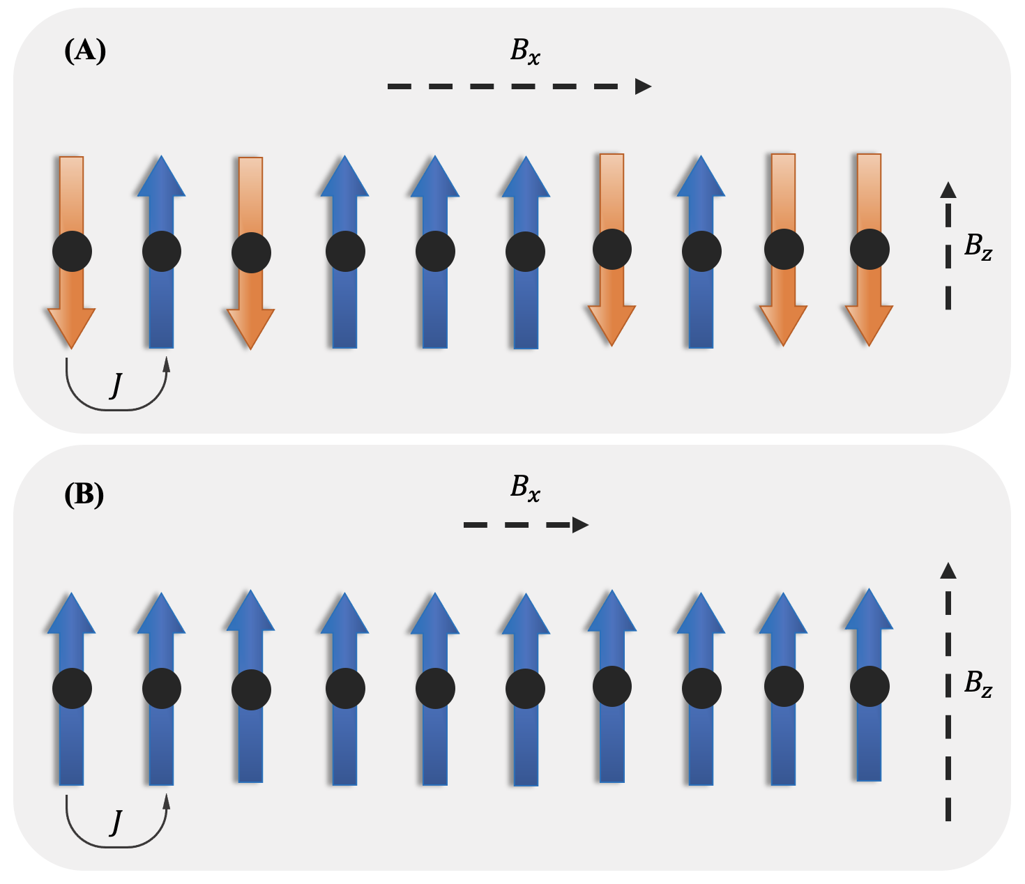
Figure 1. Ising spin chain for $N\!=\!10$ spins and coupling strength $J$. The black disks represent electrons at each site, and the arrows indicate the orientation of the spin. Box (A) shows a paramagnetic phase, with the net magnetization 1. Box (B) shows a ferromagnetic phase with net magnetization 5. The transverse field $B_{x}$, and longitudinal field $B_{z}$ are shown with vector length indicating field strength, which may be used to set the phase.

An Ising model consists of $N$ interacting electrons, each of which possess an intrinsic degree of freedom called the “spin” angular momentum. The possible values for the spin are defined with respect to an arbitrary axis, they are simply either the spin-up ($\uparrow$) or spin-down ($\downarrow$) state, which are typically expressed as a basis in Dirac notation: $\{\ket{z;\uparrow},\ket{z;\downarrow}\}$. Here, the z-axis is chosen, which is the convention for this work. A chain with $N$-spins can have $2^{N}$ unique combinations, also called configurations. These configurations form an orthonormal basis for the Schrödinger equation, resulting in a ground state wavefunction with $2^{N}$ coefficients.

Here, we consider the one-dimensional transverse Ising model (Bonfim et al., 2019) (Equation 1). It describes a system of $N$ fixed spins and is useful to understand magnetism. The spins are subjected to both a transverse and longitudinal field, denoted $B_{x}$ and $B_{z}$ respectively. Neighboring spins are coupled through an interaction term, with strength $J$. Note that we fix $J=1$ for this work. The Schrödinger eigenvalue equation, denoted as $\textbf{H}\Psi=E\Psi$, where H is the Hamiltonian (or ”total energy”) operator and $E$ is the energy eigenvalue, may be solved to obtain $\Psi$, the wavefunction, which carries all information about the system. The Hamiltonian for this system is

(1) $$\textbf{H}=-\frac{J}{N}\sum_{i=1}^{N}\sigma^{z}_{i}\sigma^{z}_{i+1}-\frac{1}{N}\sum_{i=1}^{N}\left(B_{z}\sigma^{z}_{i}+B_{x}\sigma^{x}_{i}\right)$$

where $\sigma^{z,x}$ is the corresponding Pauli matrix, and the system is subject to a periodic boundary condition. In this work, we seek to predict the ground-state wavefunction $\Psi_{0}$, corresponding to the smallest eigenvalue of the Ising Hamiltonian, $E_{0}$. Wavefunctions are subject to several requirements from the postulates of quantum mechanics (Griffiths, 2004), one of which is that the (Hilbert) vector space of states must possess an inner product $\left(\Psi_{1},\Psi_{2}\right)\equiv\braket{\Psi_{1}}{\Psi_{2}}$. Further, the states are normalized such that the overlap of a state with itself is one, $\braket{\Psi_{1}}{\Psi_{1}}=1$.

The fields $B_{x},B_{z}$ may be used to create a quantum phase transition (McCoy and Maillard, 2012). When $B_{x}<1$, the system is in the ferromagnetic phase (spins preferring all up or down in the $z-$basis). As the parameter is swept to $B_{x}>1$, the system transitions to the paramagnetic phase (either orientation is possible for each spin). Examples are shown in Figure 1. The magnetic phase of a material has enormous importance in both applied and theoretical condensed matter physics in classification of the electronic properties materials (Ashcroft and Mermin, 1976). Further, an understanding of quantum spin forms the backbone of quantum computing (Michael A. Nielsen, 2000).

3. Problem Setup

Consider a training dataset $D_{\,Tr}=\{D_{\,L}\!\cup D_{\,UL}\}$ where $D_{L}$ corresponds to a labeled dataset obtained by diagonalization solvers and $D_{UL}$ refers to an unlabeled dataset. $D_{\,L}=\{(X^{i},\mathbf{H}^{i}),\ Y^{i}\}_{i=1}^{n}$ consists of transverse and longitudinal magnetic field, $B_{x}$ and $B_{z}$ respectively, which contribute elements for the corresponding Hamiltonian matrix $\mathbf{H}$. For each data-point, the set of all the spin configurations is denoted by $C=\sigma_{1}\ \sigma_{2}\ ..\ \sigma_{2^{N}}$ where $\sigma_{i}$ represents the $i^{th}$ configuration. The ground truth $Y^{i}$ is the ground-state wavefunction $\Psi^{i}$ of the Hamiltonian $\mathbf{H}^{i}$. The set of unlabeled examples, $D_{UL}=\{(X_{U}^{i},\mathbf{H}^{i})\}_{i=1}^{m}$ can be leveraged for unsupervised training. The problem then is to learn an NN model with parameters $\mathbf{\theta}$ to predict the wavefunction $\hat{\Psi}$ of any unseen $\mathbf{H}$, i.e., $\hat{\Psi}=f_{NN}(\mathbf{\theta};\ X,\mathbf{H})$.

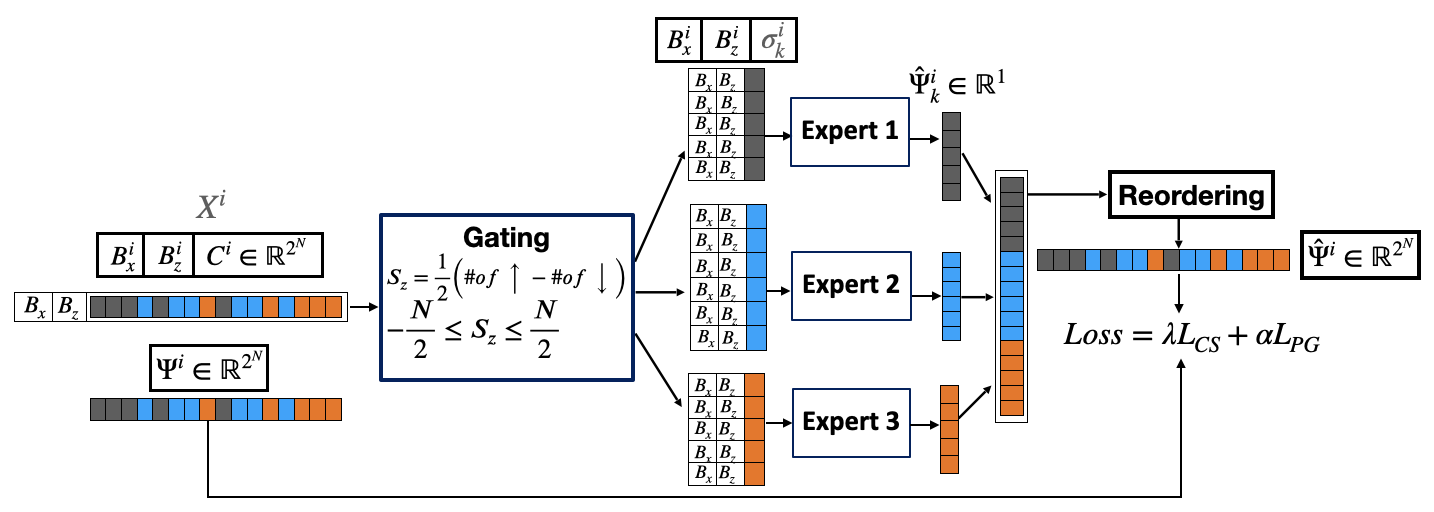
Figure 2. Physics-Guided Mixture-of-Experts (PG-MoE) pipeline. The gating component distributes the $2^{N}$ configurations and the corresponding coefficients among the experts. The configurations with the same color are mapped to the same expert. Before the loss calculation, the concatenated output from all the experts $\hat{\Psi}$ are reordered to preserve the configuration ordering of the true $\Psi$. Here, we show $N\!=\!4$ and number of experts as 3.

4. Problem Decomposition

We seek to construct a physics-guided decomposition of the input data. Any decomposition of this nature must satisfy two broad constraints: firstly, it must be physically justifiable, i.e., we may not decompose coupled quantities and, secondly, there must exist a well-defined scientific criterion that can be consistently applied to each input data point. For the Ising model, we choose the total magnetization quantum number, $S_{z}$ (Equation 2), to decompose the input space of $2^{N}$ configurations into several input sub-spaces. The orthonormality of the configuration basis vectors (Section 2) satisfies the first constraint. As for the second constraint, it is known that spin configurations with comparable values of $S_{z}$ respond similarly with respect to external physical parameters. Additionally, the value of $S_{z}$ classifies the magnetic phase of the system, and it can be used to detect the phase transition. These two qualities make $S_{z}$ a viable choice for determining the decomposition criterion. We therefore use contiguous values of $S_{z}$ to form the sub-spaces, and learn an “expert” network for each sub-space. Table 1 illustrates one such decomposition for $N=4$.

(2) $$S_{z}=\frac{(\textnormal{Total \# of}\uparrow-\textnormal{Total \# of}\downarrow)}{2}$$

Sub-spaces	configurations
$S_{z}$ = -2, -1	$\{\downarrow\downarrow\downarrow\downarrow\}$, $\{\uparrow\downarrow\downarrow\downarrow\}$, …, $\{\downarrow\downarrow\downarrow\uparrow\}$
$S_{z}$ = 0	$\{\uparrow\uparrow\downarrow\downarrow\}$, $\{\uparrow\downarrow\uparrow\downarrow\}$, …, $\{\downarrow\downarrow\uparrow\uparrow\}$
$S_{z}$ = 1, 2	$\{\uparrow\uparrow\uparrow\uparrow\}$, $\{\downarrow\uparrow\uparrow\uparrow\}$, …, $\{\uparrow\uparrow\uparrow\downarrow\}$

Table 1. One possible decomposition of the configurations based on the $S_{z}$ value for $N=4$

For the 10-spin Ising model, we train three $\mathcal{E}$ networks where the network assignment is determined according to Table 2.

Expert No.	$S_{z}$	#configurations
1	$-5\leq{S_{z}}\leq{0}$	638
2	$1\leq{S_{z}}\leq{3}$	375
3	$S_{z}={4,5}$	11

Table 2. A configuration-to-expert mapping based on the $S_{z}$ quantum number

5. Experimental Plan

5.1. Dataset

We consider an $N\!=\!10$ spin system for the Ising model. The training data $D_{\,Tr}$ comprises 300 sets of physical parameters in the range of $J\!=\!1,\ 0\!\leq\!B_{x}\!<\!1,$ and $0.06\!<\!B_{z}\!\leq\!2$, with 10 and 30 steps for $B_{x}$ and $B_{z}$ respectively. The minimum value of $B_{z}$ is set to 0.06 to eschew ground state degeneracy. From each of the 10 unique bins of $B_{x}$ values with 30 different $B_{z}$, we randomly choose 4 data points; 2 for the test set and 2 for the validation set. The resulting test set is denoted by $D_{\,T}$. The distribution of the data is listed in Table 3.

Due to the computation overhead of the exact diagonalization to produce annotated data, we also leverage unlabeled data in the training. We test the generalization of the NN for various sizes of annotated and unlabeled data. The network obtains the most supervision when all of the $B_{x}$ in $D_{\,Tr}$ are used in the annotated set $D_{\,L}$. With the decrease in the amount of data in $D_{\,L}$, the amount of supervision decreases. The most restrictive learning setting occurs when only half of the training data, i.e., from $B_{x}\!\leq\!0.5$, make up the annotated set $X$, whereas the other half, from $0.5\!<\!B_{x}\!<\!1$, make up the unlabeled set $X_{\,UL}$.

$B_{x}$	#Train (labeled)	#Train (unlabeled)	#Valid	#Test
$B_{x}\!<\!1$	130	130	20	20
$1\!\leq\!B_{x}\!\leq\!2$	0	0	0	300

Table 3. Distribution of train, test and validation data

Additionally, a dataset $D_{UT}$ is generated from the range $1\!\leq\!B_{x}\!\leq\!2$ to test the generalizability of the trained NN on unseen transverse magnetic field values. Here, $UT$ stands for Unseen Test. Specifically, we train the NN with states only in the ferromagnetic phase and hold out the paramagnetic phase states as a stress test.

5.2. Loss

Cosine Similarity Loss. A pure black-box technique to train the NN involves optimizing the network for loss–such as cosine similarity (CS) loss or mean square error (MSE)–between the true wavefunction $\Psi$ and the predicted wavefunction $\hat{\Psi}$. We prefer CS loss over MSE loss because of the normalized inner product requirement satisfied by the wavefunction. Further, the eigenstates may have an overall phase ambiguity (Sakurai, 1994) and with MSE loss the predicted states may not capture phase whereas with CS loss both the magnitude and direction for the ground-state wavefunction will be captured. For $M$ number of data-points, the cosine loss, $L_{\,CS}$, is given by Equation 3.

(3) $$L_{\,CS} =\frac{1}{M}\sum(1-\cos(\theta))$$

(4) $$\cos(\theta) =\frac{\Psi\cdot\hat{\Psi}}{\|\Psi\|\|\hat{\Psi}\|}$$

Physics Loss. The physics loss we propose to use is based on the variational principle of quantum mechanics (Griffiths, 2004) that states that the expectation value of the energy computed with any state except for the ground state will overestimate the ground state energy; $\frac{\bra{\Psi}\mathbf{H}\ket{\Psi}}{\braket{\Psi}{\Psi}}\geq E_{0}$. As such, the energy expectation value may only be a global minimum for the true ground state wavefunction - the quantity the NN learns to predict. We propose to use the NN predicted wavefunction $\ket{\hat{\Psi}}$ as a variational wavefunction in a new PG loss term such that the network must predict a wavefunction which lowers Equation 5 as much as possible.

(5) $$L_{\,PG}=\frac{1}{M}\sum\frac{\bra{\hat{\Psi}}\mathbf{H}\ket{\hat{\Psi}}}{\braket{\hat{\Psi}}{\hat{\Psi}}}$$

This loss only depends on H, which may be computed for any input without re-diagonalizing for the ground truth energy $E_{0}$.

The overall loss, $L$, is given by the Equation 6 where $\lambda_{\,CS}$ and $\lambda_{\,PG}$ are hyper-parameters to determine the scaling of each loss.

(6) $$L=\lambda_{\,CS}L_{\,CS}+\lambda_{\,PG}L_{\,PG}$$

5.3. Architectures

Baseline: Similar to (Elhamod et al., 2021), we train a feed-forward network (FFN) with $2^{N}$ nodes in the output layer to predict the ground-state wavefunction with $2^{N}$ coefficients. With the $B_{x}$ and $B_{z}$ as the inputs, the network is optimized to minimize the loss in Equation 6. This serves as our baseline architecture. Figure 3 illustrates the design of a baseline and an expert model.

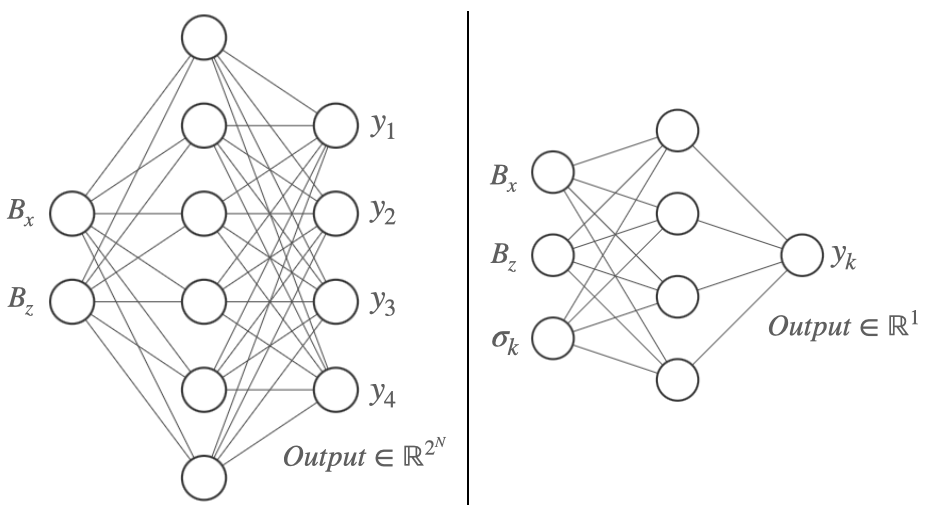
Figure 3. Example architectures for $N\!=\!2$. (Left) The baseline model is trained to predict the wavefunction coefficients $\{y_{1},\dots,y_{2^{N}}\}$ for all the configurations at the same time. (Right) The expert is tasked to predict only one coefficient $y_{k}$ corresponding to the configuration $\sigma_{k}$.

Physics-Guided Mixture-of-Experts (PG-MoE): The PG-MoE consists of a set of $\mathbf{n}$ expert networks $\textbf{$\mathcal{E}$}_{1},\dots,\textbf{$\mathcal{E}$}_{n}$, a gating component $\mathbf{G}$ and a reordering component $\mathbf{R}$. Each expert is a FFN with only 1 output node to predict one coefficient $y_{k}$ of a wavefunction corresponding to a single configuration $\sigma_{k}$. Therefore, in addition to $B_{x}$ and $B_{z}$, each expert also takes the configuration $\sigma_{k}$ as the input. We use a vector of 1s and 0s representing $\uparrow$ and $\downarrow$ to feed $\sigma_{k}$ to the NN. For example, an input {1,0,0,0} represents a configuration $\sigma=\{\uparrow\downarrow\downarrow\downarrow\}$.

Unlike the gating component used in various MoE architectures in the literature (Shazeer et al., 2017) that need a nonlinear optimization routine, our gating component is non-parameterized and does not have to be trained. When given an input with all the $2^{N}$ configurations, the gating component simply calculates the value of $S_{z}$ for each and distributes the corresponding batches of $(B_{x},B_{z},\sigma_{k})\rightarrow y_{k}$ pairs among the experts. The output from all the experts are then concatenated. As shown in Figure 2, contiguous configurations do not yield the same value of $S_{z}$ and thus alter the order of the predicted coefficients in $\hat{\Psi}$ when concatenated. Therefore, the reordering component is used to re-arrange the outputs to their original ordering before calculating the loss. The design of the PG-MoE pipeline is shown in Figure 2.

5.4. Training and Evaluation

Since the PG loss is independent of the ground-truth $\Psi$, we calculate only the PG loss for data corresponding to unlabeled data $D_{UL}$. For the annotated data $D_{L}$, the network is optimized for both the $L_{CS}$ and $L_{PG}$. We evaluate the generalization performance of NN model on the test sets $D_{T}$ and $D_{UT}$ by using mean value of the cosine similarity between our predicted wavefunction $\hat{\Psi}$ and the ground-truth $\Psi$.

5.5. Hyperparameter Optimization

5.5.1. Architecture

We sweep across different combinations of the number of hidden layers ($d$) and number of hidden units ($n$) in each layer to find the architecture that optimizes the validation performance. For the PG-MoE, we use the same architecture for the experts. For the baseline, we use a FFN with $d\!=\!2$ and $n\!=\!2000$. As for each expert, we find $d\!=\!2$ and $n\!=\!200$ to be ideal.

5.5.2. Training

Given the small amount of data, we use a small batch size of 8 for all of the training. The loss scaling factors, ($\lambda_{\,CS}$, $\lambda_{\,PG}$), that yield the best validation performance for the baseline and the PG-MoE are (1, 100) and (100, 200) respectively. We train both the baseline and PG-MoE with stochastic gradient descent (SGD) (Bottou et al., 2018). We find the training of PG-MoE to be unstable, resulting in the oscillations in the gradient descent, and three ways to mitigate the instability: (1) using a small learning rate, (2) using a momentum (Sutskever et al., 2013) of 0.99, and (3) decaying the learning rate by a factor of 0.987 when the validation loss does not improve for 8 consecutive epochs. For all of the training, we use early stopping (Caruana et al., 2000)–training is stopped when the validation performance on the seen data does not improve for 30 epochs. This avoids overfitting of the networks, especially the baseline architecture, which consisting of $\footnotesize\sim$6 million parameters.

Another key finding is that if PG loss is introduced early in the learning process, the network not only runs the risk of getting stuck in local minima but also the convergence becomes slower. As a result, we only use the cosine loss for the first few epochs before switching to the combination of both the loss components in Equation 6. This correspond to $epoch\!=\!80$ and $epoch\!=\!55$ for the baseline and PG-MoE when both are trained for a maximum of 300 and 400 epochs respectively. For each experimental setup, we either run the models for five distinct seeds and choose the one that performs the best across all runs for that study or use mean and standard deviation to combine the five numbers.

6. Results

6.1. Evaluation of Decomposition

Figure 4 compares the generalization performance of the baseline and PG-MoE on the unseen test set $D_{\,UT}$. Both the networks are trained on different subsets of labeled data and optimized for CS loss (i.e., $\lambda_{\,PG}\!=\!0$). Although PG-MoE outperforms the baseline for all categories of training data, the gap between the two increases as the number of labeled data in $D_{\,L}$ decreases from 260 to 130. For $D_{\,L}\!:B_{x}\!<\!0.5$, the mean CS of the PG-MoE on $D_{\,UT}$ is better than baseline by $2\%$ while requiring $2\times$ fewer epochs to train. On average, PG-MoE requires $\sim$60$\%$ fewer epochs than the baseline to achieve similar test performance.

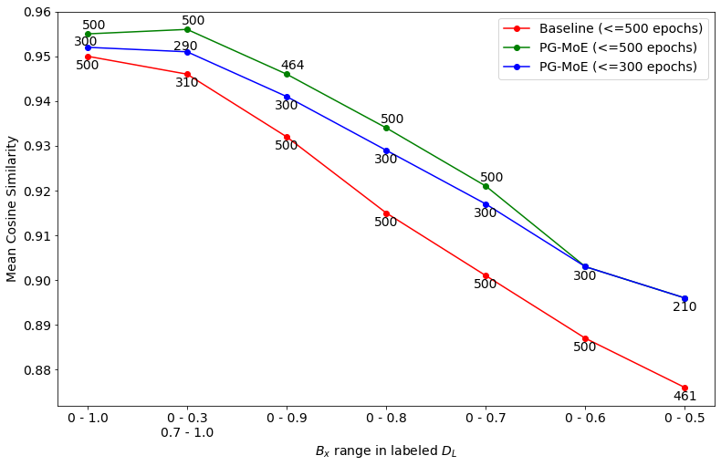
Figure 4. Mean cosine similarity on unseen test data $D_{\,UT}$ of the baseline and the PG-MoE networks when trained for 300 and 500 epochs. The annotated labels show the epoch where the training early stopped.

Model	Architecture	#params	CS (w/o $L_{PG}$)		CS (with $L_{PG}$)
			$B_{x}\!<\!1$	$B_{x}\!>\!1$	$B_{x}\!<\!1$	$B_{x}\!>\!1$
Baseline	$d\_2\_n\_2000$	6093024	$0.996\pm 0.0008$	$0.874\pm 0.0028$	$1.000\pm 0.000$	$0.981\pm 0.0003$
PG-MoE	$d\_2\_n\_200$	39903	$0.996\pm 0.0008$	${0.882\pm 0.0083}$	$1.000\pm 0.000$	${0.977\pm 0.0044}$

Table 4. Comparison of cosine similarity of the Baseline and PG-MoE networks on the $D_{\,T}$ ($B_{x}\!<\!1$) and $D_{\,UT}$ ($B_{x}\!>\!1$) test sets. $d$ and $n$ correspond to the number of hidden layers and the number of neurons in each layer of the NN.

6.2. Effect of Physics Loss

Table 4 provides a more detailed comparison of the baseline and the PG-MoE model on both the seen and the unseen test ranges: $D_{\,T}$ and $D_{\,UT}$. To determine how sensitive the networks are, we run both models for 5 different seed values and compute the mean and standard deviation of cosine similarity for each. When trained on $D_{\,L}\!:\!B_{x}\!<\!0.5$ and $D_{\,UL}\!:\!0.5\!<\!B_{x}\!<\!1$, PG-MoE requires $\sim$150$\times$ lesser parameters than the baseline architecture to achieve competitive performance. For both networks, PG loss yields a perfect cosine similarity on the seen test set $D_{\,T}$. The test performance on $D_{\,UT}$ also improves by $\sim$12$\%$ for both the baseline and the PG-MoE. It is worth noting that the standard deviation in CS for both models is much lower when they are trained with PG loss. This demonstrates how PG loss helps in limiting the convergence region, making the training less sensitive to variations.

Another observation is that the PG-MoE has a larger standard deviation than the baseline for the unseen test $D_{\,UT}$. This is because, as mentioned in Section 5.5.2, the training procedure of PG-MoE is susceptible to oscillations in the gradient descent, leading to variations in performance. Note that the optimization process of training multiple experts in PG-MoE is much more complex than training a single baseline, where the gradient descent of each expert to their respective local minima may show competing directions. Also note that the selection of the loss scaling factors, $\lambda_{\,CS}$ and $\lambda_{\,PG}$ in Equation 6, at different stages of PG-MoE training can influence variations in performance. Further algorithmic improvements in training mixture of experts are needed to reduce the variance in PG-MoE results.

6.3. Annotated Data and Generalization

As shown in Table 5, PG loss not only helps generalize better in the unseen test regime, it also helps achieve a consistent test performance as the amount of the labeled data decreases. When the amount of supervised data is decreased by 50%, i.e., from 260 to 130, PG-MoE optimized only with $L_{CS}$ shows a $\sim$6% drop in performance whereas the network trained with the PG loss has similar performance.

It is also worth noting that the test performance on unseen $B_{x}\!>1$ is not solely related to the number of labeled data-points. Consider two ranges of $D_{L}$: $B_{x}\!<0.3\cup 0.7\!<\!B_{x}\!<\!1$ and $B_{x}\!<\!0.6$. Although both have 156 labeled data, the test performance for the former range is better than the latter by $\footnotesize\sim$5%, when optimized with the black-box loss. This is because the former range includes $B_{x}$ values close to the ferromagnetic to paramagnetic transition phase (c.f. Section 2), which happens at $B_{x}\!=\!1$. The inclusion of these data points aids the model’s extrapolation for the $D_{UT}$ test set, that primarily consists of data in the paramagnetic phase.

$\mathbf{|D_{L}|}$	$\mathbf{B_{x}}$ Range		CS (w/o $L_{PG}$)		CS (with $L_{PG}$)
	$\mathbf{D_{L}}$	$\mathbf{D_{UL}}$	$\mathbf{B_{x}}\!<\!1$	$\mathbf{B_{x}}\!>\!1$	$\mathbf{B_{x}}\!<\!1$	$\mathbf{B_{x}}\!>\!1$
260	0 - 1.0	N/A	0.998	0.952	1.000	0.976
156	0 - 0.3; 0.7 - 1	0.3 - 0.7	0.998	0.952	1.000	0.980
234	0 - 0.9	0.9 - 1	0.999	0.946	1.000	0.977
208	0 - 0.8	0.8 - 1	0.998	0.933	1.000	0.970
182	0 - 0.7	0.7 - 1	0.998	0.919	1.000	0.974
156	0 - 0.6	0.6 - 1	0.997	0.903	1.000	0.978
130	0 - 0.5	0.5 - 1	0.996	0.894	1.000	0.981

Table 5. Cosine similarity for the seen ($B_{x}\!<\!1$) and unseen test sets ($B_{x}\!>\!1$) for various amounts of labeled data $D_{\,L}$ in the training set. The CS w/o $L_{\,PG}$ column represents PG-MoE optimized with only the black-box loss.

6.4. Effect of $B_{x},B_{z}$ in Cosine Similarity

The wavefunction prediction is more accurate (in terms of CS) for some ($B_{x},B_{z}$) pairs, whereas for others, it is particularly challenging. The following observations are made from Figure 5:

1. For any given $B_{x}$, $B_{z}=0.06$ (lowest value) yields the worst CS, and the performance improves as we increase the value of $B_{z}$.

2. If we compare the CS for the same $B_{z}$, the performance consistently reduces as we increase $B_{x}$ from 1.05 to 2.0.

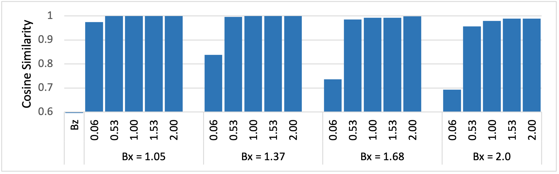
Figure 5. Cosine similarity for different $B_{x}$ and $B_{z}$ values in the $D_{\,UT}$ test data.

It is intriguing that this observation is very consistent with the physical idea of the phase transition. A small but finite value of $B_{z}$ is enough to align the spins along $z$ direction, and applying a magnetic field along $x$ direction could turn the spin’s orientation away from $z$ direction. In other words, $B_{z}$ and $B_{x}$ are in fact two competing energy scales to determine the spin orientation. As a result, the stronger $B_{x}$ is, the fluctuations introduced into the system are larger, which makes the prediction more challenging, and hence the performance is lower.

	$\mathcal{E}_{1}$	$\mathcal{E}_{2}$	$\mathcal{E}_{3}$	$\mathcal{E}_{4}$	CS (with $L_{\,PG}$)
Random	$S_{z}$ = {-3, -2, 1, 5}	$S_{z}$ = {-4, 0, 4}	$S_{z}$ = {-5, -1, 2, 3}	-	${0.859\pm 0.0341}$
Only-1	-5 ¡ $S_{z}$ ¡ 5	-	-	-	${0.970\pm 0.0083}$
PG-MoE1	$S_{z}$ ¡ 0	$S_{z}\!\geq 0$	-	-	${0.964\pm 0.0167}$
PG-MoE2	$S_{z}$ ¡ 0	$S_{z}$ = 0	$S_{z}$ ¿ 0	-	${0.967\pm 0.0044}$
PG-MoE3	$S_{z}$ ¡= 0	$S_{z}$ = {1, 2, 3}	$S_{z}$ = {4, 5}	-	${\mathbf{0.977\pm 0.0044}}$
PG-MoE4	$S_{z}$ ¡= 0	$S_{z}$ = {1, 2, 3}	$S_{z}$ = 4	$S_{z}$ = 5	${0.973\pm 0.0031}$

Table 6. Mean and standard deviation of cosine similarity on test set $D_{\,UT}$ for various $S_{z}\!\rightarrow\mathcal{E}_{i}$ mappings.

7. Ablation Studies

We design a number of ablation experiments to explore the impact of various design decisions.

7.1. Unlabeled Data and Generalization

While keeping the labeled data $D_{L}$ fixed, we vary the amount of unlabeled data in the training from $0.5\!\leq B_{x}\!<1.5$ and test the generalization on the $D_{UT}$ dataset. As shown in Figure 6, PG-MoE trained with PG loss but with no unlabeled data is only slightly better than the one trained only with the black-box loss. The mean CS on the test set consistently increases with the increase in the amount of unlabeled data. The mean CS of the PG-MoE trained with 260 unlabeled data-points is $13\%$ better than the model trained with no unlabeled input.

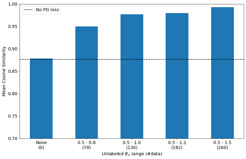
Figure 6. Cosine similarity of PG-MoE on unseen test data $1\!<\!B_{x}\!<2$ when trained with annotated data with $B_{x}\!<\!0.5$ and different subsets of unlabeled data from $0.5\!<B_{x}\!<1.5$. Other than the dashed black line, all the other numbers are from PG-MoE optimized with both CS and PG loss.

7.2. Comparison of Different Decomposition Strategies

In Table 6, we compare the cosine similarity of six types of expert assignments on the unseen test data $D_{UT}$. In addition to the various ways in which we can partition the contiguous values of $S_{z}$, we also evaluate two comparatively limiting cases of the $S_{z}\rightarrow\mathcal{E}$ mapping: (1) randomly grouping $S_{z}$ in 3 sub-groups for 3 expert architectures, and (2) assigning all the configurations, i.e., all the $S_{z}$, to only one architecture. For the other partitions, we vary the number of experts from 2 (PG-MoE₁) to 4 (PG-MoE₄). PG-MoE₃ has the same decomposition as in Table 2. For each decomposition, we run the resulting models for 5 distinct seed values and compute the mean and standard deviation of CS for each.

When optimized with the PG-loss, the random mapping of $S_{z}\!\rightarrow\!\mathcal{E}_{i}$ not only yields the worst test cosine similarity, it also has $\sim$8$\times$ more spread than PG-MoE₃. The PG-MoE models become less susceptible to randomization (compare the deviation from PG-MoE₁ through PG-MoE₄) as $S_{z}\!\geq\!0$ is sub-divided. We believe this is related to the fact that the phase transition is expected to occur in the range $0\!\leq S_{z}\!\leq N/2$, resulting in large variations in the output coefficients. This makes learning in this range more difficult than learning in the $S_{z}\!\leq\!0$ regime, which comprises of very low coefficient values in the wavefunction. As a result, dividing $S_{z}\!\geq\!0$ into multiple partitions helps in decomposing the overall task into simpler and smaller tasks, thus resulting in better CS values of PG-MoE₂, PG-MoE₃, and PG-MoE₄ relative to PG-MoE₁. Nevertheless, over-partitioning $S_{z}\geq 0$ also reduces the training sizes available to each expert and make them under-representative, thus degrading performance. As a result, we can see that the cosine similarity of PG-MoE₄ is slightly smaller than that of PG-MoE₃.

7.3. Hyperparameter Selection

We evaluate the impact of alternate hyperparameter selection with our chosen values in the first row of Table 7. Out of five hyperparameters, namely (i) learning rate (lr), (ii) epoch where PG-loss is introduced (pge), (iii) decay factor for the learning rate scheduler ($\gamma$), (iv) momentum (mom) for SGD, and (v) loss scaling factors ($\lambda_{\,CS}$, $\lambda_{\,PG}$), we vary one parameter at a time keeping others constant. The table’s empty cells imply that the values in the first row are used.

It is crucial to not train the model with the PG-loss from the very beginning, i.e., pge = 0. This is true even for the baseline architecture, and is consistent with the findings in (Elhamod et al., 2021). We find PG-MoE architecture to be prone to oscillations, therefore, it skips the global minima in the absence of momentum (mom = 0) or learning rate decay ($\gamma\!=\!0$), or when the initial learning rate is high ($lr\!=\!0.0004$). While both mom and $\gamma$ has a small search space of {0.9, 0.985, 0.987, 0.99}, the parameters ($\lambda_{\,CS}$, $\lambda_{\,PG}$) are particularly difficult to tune. We make two observations while tuning for these scaling factors. First, since the cosine loss can get to a very small value at the later stages of the training, $\lambda_{\,CS}$=1 can lead to vanishing gradients, we, therefore, set this to a high value and empirically find $\lambda_{\,CS}$=100 to be the best choice. (In future work, we will implement adaptive tuning to choose the best scalars). Second, we find that the network is able to extrapolate better when $\lambda_{\,CS}\!<\lambda_{\,PG}$. This can be seen when we compare the scale factor (100, 200) with (100, 100) and (100, 50) in the Table 7.

lr	pge	$\gamma$	mom	($\mathbf{\lambda_{CS}}$, $\mathbf{\lambda_{PG}}$)	$B_{x}\!<1$	$B_{x}\!>1$
0.0003	55	0.987	0.99	(100, 200)	1.000	0.981
0.0002					1.000	0.966
0.0004					0.502	0.794
	0				-1.000	-0.963
	30				0.498	0.813
		0			0.502	0.715
		0.9			1.000	0.974
		0.985			1.000	0.979
			0		0.996	0.955
			0.9		1.000	0.963
				(1,1)	0.999	0.955
				(100, 50)	1.000	0.954
				(100, 100)	1.000	0.973
				(50, 200)	1.000	0.979

Table 7. Effect of changing the hyperparameters in PG-MoE training on the testing performance. The first row corresponds to the choices that yield the best cosine similarity on the test sets when the network is trained with $L_{\,PG}$.

8. Related Work

Quantum Ising Model. Neural networks have been employed to study the quantum Ising model previously. One commonly used method is the restricted Boltzmann machine (RBM) that is designed to learn the distributions of coefficients for spin configurations in the ground state using a generic model. Success has been shown to reproduce the results of physical properties including the magnetization, spin-spin correlation function, and entanglement entropy (Hinton and Salakhutdinov, 2006; Deng et al., 2017; Amin et al., 2018; Iso et al., 2018; Torlai and Melko, 2016; Morningstar and Melko, 2017; D’Angelo and Böttcher, 2020). These studies focused on learning particular physical properties instead of the ground state wave function directly. Moreover, the PG loss functions for unlabeled data were not considered.

Physics-Guided Machine Learning. Physics-guided machine learning is becoming an increasingly common method for solving problems in a wide variety of physics dependent fields such as fluid mechanics (Cai et al., 2021; Ling et al., 2016; Raissi et al., 2018; Wang et al., 2020a), electromagnetism (Jin et al., 2021; Zhang et al., 2021; Noakoasteen et al., 2020), thermodynamic modeling (Ihunde and Olorode, 2022; Zhang et al., 2020; Amini Niaki et al., 2021; Patel et al., 2020), and even in medical engineering (Sahli Costabal et al., 2020). By imposing physical constraints to respect any symmetries (Wang et al., 2020b), invariances (Ling et al., 2016), or conservation principles (Beucler et al., 2019), researchers are able to constrain the space of admissible solutions to a manageable size even with a few hundred data-points.

In materials science, most important quantum phenomena are dominated by the ground state solution of the Schrödginer equation. Obtaining the ground state solution for a system with many interacting electrons remains one of the most challenging problems in theoretical physics. A traditional approach is to build up a trial function with multiple parameters, namely an ansatz, to represent the ground state solution, and the parameters in the ansatz are determined by satisfying the physical constraints. Studies of deep learning models using the physics-guided ansatz as the learning target have been performed (Hermann et al., 2020; Luo and Clark, 2019), but the applicability of the same ansatz to radically different systems is unclear.

The Ising model has also been studied recently in CoPhy-PGNN (Elhamod et al., 2021). As is the case in that work, we leverage both unlabeled data and physics loss for better extrapolation. But unlike their neural network, which is also the basis of our baseline architecture, our proposed PG-MoE is scalable for large physical systems. CoPhy-PGNN trains a neural network to predict the entire ground state wavefunction for an $N\!=\!4$ system. With just $2^{4}=16$ coefficients in the output, it is a much smaller problem as compared to the $N\!=\!10$ system with $2^{10}\!=\!1024$ output values in the wavefunction. With our baseline comparison, we show that PG-MoE can achieve similar test performance as the architecture in CoPhy-PGNN (Elhamod et al., 2021) while being smaller by more than two orders of magnitude. Additionally, the PG loss presented in CoPhy-PGNN applies to any eigenvector whereas our new loss is true for only the vector we seek to predict.

Problem Decomposition. Extreme classification tasks in domains like computer vision and NLP have seen a scaling issue similar to Quantum Mechanics. The challenge essentially originates from the necessity to train a deep model to predict millions of classes, which result in a memory and computation explosion in the last output layer. MACH (Merged-Average Classification via Hashing) (Medini et al., 2019) employs a hashing based divide-and-conquer algorithm to map $K$ classes into $B$ buckets, where $B\!\ll\!K$, and learns a classifier for each bucket. Another method of scaling large neural networks is to use a mixture-of-experts (MoE) (Jacobs et al., 1991; Eigen et al., 2013; Shazeer et al., 2017), which involves training multiple expert networks or learners to handle a subset of the entire training set. A gating network is trained to distribute the inputs and combine the corresponding outputs to produce a final output. Although our idea of problem decomposition share the same underlying principle of divide-and-conquer, our approach is different in two respects: (1) we use physics to design the input sub-spaces, and (2) the gating component in our proposed PG-MoE need not be learned and involves a computationally cheap operation (Equation 2).

9. Conclusions and Future Work

We have demonstrated the use of physics to decompose a complex machine learning problem into smaller problems, which avoids the exponential growth in the neural network’s output layer, which is prevalent in high-dimensional eigenvalue problems. The approach leads to learning multiple parameter-efficient expert networks, one for each component problem sub-space, to yield a Physics-Guided Mixture-of-Experts (PG-MoE). The PG-MoE in our case study is $\sim$150$\times$ smaller but has similar extrapolation ability as the model trained on the complex problem. Along with decomposition, we also employed fundamental quantum mechanics in designing a loss function that included the variational method, which better guides the learning of the eigenvector we seek to predict. Notably, while we show the efficacy of our approach for the Ising chain model for 10 spins, our solution is scalable for much larger physical systems. Our work has useful connotations in other scientific applications like quantum spin problems in two-dimensions, interacting fermionic system, and physical systems governed by partial differential equations which possess matrix representation.

For future work, an important topic is to characterize an upper bound for the scalability of the PG-MoE approach, which may be studied by increasing the total number of spins as well as promoting the system to two-dimensions. We will also focus on improving the stability and sensitivity of PG-MoE training. Another intriguing direction is to incorporate traditional theoretical approaches like the quantum Monte Carlo method to train the PG-MoE for large systems. Because labeled data is not easily obtained in these cases, the advantages of PG-MoE for efficient neural network architecture and PG loss for extrapolation would get further tested.

References

- (1)
- Amin et al. (2018) Mohammad H. Amin, Evgeny Andriyash, Jason Rolfe, Bohdan Kulchytskyy, and Roger Melko. 2018. Quantum Boltzmann Machine. Phys. Rev. X 8 (May 2018), 021050. Issue 2. https://doi.org/10.1103/PhysRevX.8.021050
- Amini Niaki et al. (2021) Sina Amini Niaki, Ehsan Haghighat, Trevor Campbell, Anoush Poursartip, and Reza Vaziri. 2021. Physics-informed neural network for modelling the thermochemical curing process of composite-tool systems during manufacture. Computer Methods in Applied Mechanics and Engineering 384 (Oct 2021), 113959. https://doi.org/10.1016/j.cma.2021.113959
- Ashcroft and Mermin (1976) Neil W. Ashcroft and David N. Mermin. 1976. Solid State Physics. Holt-Saunders.
- Beucler et al. (2019) Tom Beucler, Stephan Rasp, Michael Pritchard, and Pierre Gentine. 2019. Achieving conservation of energy in neural network emulators for climate modeling. arXiv preprint arXiv:1906.06622 (2019).
- Bonfim et al. (2019) Oz F. de Alcantara Bonfim, B. Boechat, and J. Florencio. 2019. Ground-state properties of the one-dimensional transverse Ising model in a longitudinal magnetic field. Physical Review E 99, 1 (Jan 2019). https://doi.org/10.1103/physreve.99.012122
- Bottou et al. (2018) Léon Bottou, Frank E Curtis, and Jorge Nocedal. 2018. Optimization methods for large-scale machine learning. Siam Review 60, 2 (2018), 223–311.
- Cai et al. (2021) Shengze Cai, Zhiping Mao, Zhicheng Wang, Minglang Yin, and George Em Karniadakis. 2021. Physics-informed neural networks (PINNs) for fluid mechanics: A review. arXiv:2105.09506 [physics.flu-dyn]
- Caruana et al. (2000) Rich Caruana, Steve Lawrence, and C Giles. 2000. Overfitting in neural nets: Backpropagation, conjugate gradient, and early stopping. Advances in neural information processing systems 13 (2000).
- D’Angelo and Böttcher (2020) Francesco D’Angelo and Lucas Böttcher. 2020. Learning the Ising model with generative neural networks. Physical Review Research 2, 2 (2020), 023266.
- Deng et al. (2017) Dong-Ling Deng, Xiaopeng Li, and S. Das Sarma. 2017. Quantum Entanglement in Neural Network States. Phys. Rev. X 7 (May 2017), 021021. Issue 2. https://doi.org/10.1103/PhysRevX.7.021021
- Eigen et al. (2013) David Eigen, Marc’Aurelio Ranzato, and Ilya Sutskever. 2013. Learning factored representations in a deep mixture of experts. arXiv preprint arXiv:1312.4314 (2013).
- Elhamod et al. (2021) Mohannad Elhamod, Jie Bu, Christopher Singh, Matthew Redell, Abantika Ghosh, Viktor Podolskiy, Wei-Cheng Lee, and Anuj Karpatne. 2021. CoPhy-PGNN: Learning Physics-guided Neural Networks with Competing Loss Functions for Solving Eigenvalue Problems. arXiv:2007.01420 [cs.LG]
- Griffiths (2004) David J. Griffiths. 2004. Introduction to Quantum Mechanics (2nd Edition). Pearson Prentice Hall.
- Hermann et al. (2020) Jan Hermann, Zeno Schätzle, and Frank Noé. 2020. Deep-neural-network solution of the electronic Schrödinger equation. Nature Chemistry 12, 10 (Sep 2020), 891–897. https://doi.org/10.1038/s41557-020-0544-y
- Hinton and Salakhutdinov (2006) Geoffrey E. Hinton and Ruslin R. Salakhutdinov. 2006. Reducing the Dimensionality of Data with Neural Networks. Science 313, 5786 (2006), 504–507. https://doi.org/10.1126/science.1127647 arXiv:https://science.sciencemag.org/content/313/5786/504.full.pdf
- Ihunde and Olorode (2022) Thelma Anizia Ihunde and Olufemi Olorode. 2022. Application of physics informed neural networks to compositional modeling. Journal of Petroleum Science and Engineering 211 (2022), 110175. https://doi.org/10.1016/j.petrol.2022.110175
- Iso et al. (2018) Satoshi Iso, Shotaro Shiba, and Sumito Yokoo. 2018. Scale-invariant feature extraction of neural network and renormalization group flow. Physical review E 97, 5 (2018), 053304.
- Jacobs et al. (1991) Robert A Jacobs, Michael I Jordan, Steven J Nowlan, and Geoffrey E Hinton. 1991. Adaptive mixtures of local experts. Neural computation 3, 1 (1991), 79–87.
- Jin et al. (2021) Wentian Jin, Shaoyi Peng, and Sheldon X.-D. Tan. 2021. Data-Driven Electrostatics Analysis based on Physics-Constrained Deep learning. In 2021 Design, Automation Test in Europe Conference Exhibition (DATE). 1382–1387. https://doi.org/10.23919/DATE51398.2021.9474231
- Ling et al. (2016) Julia Ling, Andrew Kurzawski, and Jeremy Templeton. 2016. Reynolds averaged turbulence modelling using deep neural networks with embedded invariance. Journal of Fluid Mechanics 807 (2016), 155–166.
- Luo and Clark (2019) Di Luo and Bryan K. Clark. 2019. Backflow Transformations via Neural Networks for Quantum Many-Body Wave Functions. Physical Review Letters 122, 22 (Jun 2019). https://doi.org/10.1103/physrevlett.122.226401
- McCoy and Maillard (2012) Barry M. McCoy and Jean-Marie Maillard. 2012. The Importance of the Ising Model. Progress of Theoretical Physics 127, 5 (May 2012), 791–817. https://doi.org/10.1143/ptp.127.791
- Medini et al. (2019) Tharun Medini, Qixuan Huang, Yiqiu Wang, Vijai Mohan, and Anshumali Shrivastava. 2019. Extreme classification in log memory using count-min sketch: A case study of Amazon search with 50M products. arXiv preprint arXiv:1910.13830 (2019).
- Michael A. Nielsen (2000) Isaac L. Chuang Michael A. Nielsen. 2000. Quantum Computation and Quantum Information. Cambrige University Press.
- Morningstar and Melko (2017) Alan Morningstar and Roger G Melko. 2017. Deep learning the ising model near criticality. The Journal of Machine Learning Research 18, 1 (2017), 5975–5991.
- Noakoasteen et al. (2020) Oameed Noakoasteen, Shu Wang, Zhen Peng, and Christos Christodoulou. 2020. Physics-Informed Deep Neural Networks for Transient Electromagnetic Analysis. IEEE Open Journal of Antennas and Propagation 1 (2020), 404–412. https://doi.org/10.1109/OJAP.2020.3013830
- Patel et al. (2020) Ravi G. Patel, Indu Manickam, Nathaniel A. Trask, Mitchell A. Wood, Myoungkyu Lee, Ignacio Tomas, and Eric C. Cyr. 2020. Thermodynamically consistent physics-informed neural networks for hyperbolic systems. arXiv:2012.05343 [math.NA]
- Raissi et al. (2018) Maziar Raissi, Alireza Yazdani, and George Em Karniadakis. 2018. Hidden Fluid Mechanics: A Navier-Stokes Informed Deep Learning Framework for Assimilating Flow Visualization Data. arXiv:1808.04327 [cs.CE]
- Sahli Costabal et al. (2020) Francisco Sahli Costabal, Yibo Yang, Paris Perdikaris, Daniel E. Hurtado, and Ellen Kuhl. 2020. Physics-Informed Neural Networks for Cardiac Activation Mapping. Frontiers in Physics 8 (2020). https://doi.org/10.3389/fphy.2020.00042
- Sakurai (1994) Jun John Sakurai. 1994. Modern quantum mechanics; rev. ed. Addison-Wesley, Reading, MA.
- Shazeer et al. (2017) Noam Shazeer, Azalia Mirhoseini, Krzysztof Maziarz, Andy Davis, Quoc Le, Geoffrey Hinton, and Jeff Dean. 2017. Outrageously large neural networks: The sparsely-gated mixture-of-experts layer. arXiv preprint arXiv:1701.06538 (2017).
- Sutskever et al. (2013) Ilya Sutskever, James Martens, George Dahl, and Geoffrey Hinton. 2013. On the importance of initialization and momentum in deep learning. In International conference on machine learning. PMLR, 1139–1147.
- Torlai and Melko (2016) Giacomo Torlai and Roger G Melko. 2016. Learning thermodynamics with Boltzmann machines. Physical Review B 94, 16 (2016), 165134.
- Wang et al. (2020a) Rui Wang, Karthik Kashinath, Mustafa Mustafa, Adrian Albert, and Rose Yu. 2020a. Towards Physics-informed Deep Learning for Turbulent Flow Prediction. arXiv:1911.08655 [physics.comp-ph]
- Wang et al. (2020b) Rui Wang, Robin Walters, and Rose Yu. 2020b. Incorporating symmetry into deep dynamics models for improved generalization. arXiv preprint arXiv:2002.03061 (2020).
- Zhang et al. (2020) Jiaxin Zhang, Congjie Wei, and Chenglin Wu. 2020. Thermodynamic Consistent Neural Networks for Learning Material Interfacial Mechanics. arXiv:2011.14172 [cs.CE]
- Zhang et al. (2021) Pan Zhang, Yanyan Hu, Yuchen Jin, Shaogui Deng, Xuqing Wu, and Jiefu Chen. 2021. A Maxwell’s Equations Based Deep Learning Method for Time Domain Electromagnetic Simulations. IEEE Journal on Multiscale and Multiphysics Computational Techniques 6 (2021), 35–40. https://doi.org/10.1109/JMMCT.2021.3057793