The Transfer Performance of Economic Models

Abstract.

Economists often estimate models using data from a particular domain, e.g. estimating risk preferences in a particular subject pool or for a specific class of lotteries. Whether a model’s predictions extrapolate well across domains depends on whether the estimated model has captured generalizable structure. We provide a tractable formulation for this “out-of-domain” prediction problem and define the transfer error of a model based on how well it performs on data from a new domain. We derive finite-sample forecast intervals that are guaranteed to cover realized transfer errors with a user-selected probability when domains are iid, and use these intervals to compare the transferability of economic models and black box algorithms for predicting certainty equivalents. We find that in this application, the black box algorithms we consider outperform standard economic models when estimated and tested on data from the same domain, but the economic models generalize across domains better than the black-box algorithms do.

1. Introduction

When we estimate models on data, we often hope that the estimated model will be useful for making predictions in domains beyond the specific context from which the data were drawn. For example, we might estimate a pricing model on purchase data from one population of consumers and use it to predict demand in a new population with different demographics, or estimate a model of risk preferences on choices over insurance plans and use it to predict choice over state-contingent consumption bundles. This paper provides a tractable approach for evaluating cross-domain transfer performance, which (among other uses) can be applied to compare the generalizability of economic models and black box machine learning methods. Specifically, we derive finite-sample forecast intervals for a model’s out-of-domain error, and then use them to evaluate the transferability of models and black box algorithms for predicting risk preferences over binary lotteries. In this application, economic models transfer more reliably than two popular black box algorithms.

The question of how well a model trained on data from one domain will perform in a new domain dates back at least to Haavelmo (1944), and is a focus of work on external validity (Pearl and Bareinboim, 2011; Tipton and Olsen, 2018; Chassang and Kapon, 2022) and out-of-distribution prediction (Shen et al., 2021). Understanding the transfer performance of various models is of increased relevance given the recent popularity of black-box machine learning methods within economics (Hofman et al., 2021). Black box methods (such as random forest algorithms) have been widely criticized for their lack of generalizability, and one reason some economists prefer structured economic models is the belief that such models are more likely to capture fundamental regularities that apply in a wide variety of domains (Coveney et al., 2016; Athey, 2017; Manski, 2021). On the other hand, economic models have also been criticized for failing to generalize. For example, although the theoretical literature on risk preferences includes some of the most widely used models in economics, it has been singled out as a setting where large datasets and flexible black box methods may help identify new regularities and more complete models (e.g., Plonsky et al. 2019, Ke et al. 2020, and Peterson et al. 2021).

Our conceptual framework, described in Section 2, is an extension of the usual “out-of-sample” evaluation to “out-of-domain” evaluation. In the standard out-of-sample test, a model’s free parameters are estimated on a training sample, and the predictions of the estimated model are evaluated on a test sample, where the observations in the training and test samples are drawn from the same distribution. We depart from this framework by supposing that the distribution of the data varies across a set of “domains,” but that these domain-specific distributions are themselves drawn iid. While this assumption is restrictive, and rules out some interesting prediction problems, we view it as a useful first step that yields easy-to-apply procedures which we then generalize.

We consider several measures for a model’s transferability across domains. First, we ask how well the model will predict in a sample from an as-yet unobserved target domain. We call this the model’s transfer error. Since the size of the raw transfer error can be difficult to interpret, we then define a model’s normalized transfer error to be the ratio of its transfer error to a proxy for the best achievable error on the sample from the target domain. Finally, we ask how much is lost by transferring a model across domains instead of re-estimating the model’s parameters on the new domain of interest. We call this the model’s transfer deterioration. The first two measures can help select between models for making predictions in new domains; the third measure indicates the value of obtaining data from the target domain.

Section 3 shows how to construct forecast intervals with guaranteed coverage probability for these measures, using a meta-data set of samples from already observed domains. To construct a forecast interval for the estimated model’s transfer error on the new domain, we split the observed domains in the meta-data set into training and test domains. We estimate the parameters of the model on the samples from the training domains and evaluate its transfer error on each of the test domains. Pooling these transfer errors across different choices of training and test domains yields an empirical distribution of transfer errors. We show that for every quantile $\tau$, the interval bounded by the $\tau$-th and $(1-\tau)$-th quantiles of the pooled transfer error is a valid forecast interval for the transfer error on a new, unseen domain. The same method yields forecast intervals for our other two measures as well. We next relax our iid sampling assumption, deriving a modified procedure for cases where the distributions in training domains are drawn iid from one distribution, while the distribution in the target domain is drawn from another. We implement this procedure and the other methods described in this paper in an R package (transferUQ), available on Github.

Section 4 uses our results to evaluate the transferability of predictions of certainty equivalents for binary lotteries. The samples correspond to observations from different subject pools, so a model’s transfer error describes how well it predicts outcomes in one subject pool when estimated on data from another. We evaluate two models of risk preferences, expected utility and cumulative prospect theory, and two popular black box machine learning algorithms, random forest and kernel regression. We first consider a standard out-of-sample test, where the training and test data are drawn from the same subject pool, and find that the black box algorithms slightly outperform the economic models out-of-sample for most of the subject pools. This could be because the black box learns general properties of the map from lotteries to certainty equivalents that the economic models miss. Alternatively, it could be that the gains of the black boxes are specific to the within-domain prediction task, and do not correspond to improved generalizability. Transfer performance points to the latter: while the forecast intervals for the black box algorithms and economic models overlap, the forecast intervals for the black box methods are wider, and their upper bounds are substantially higher. For example the 5th and 95th percentiles of the pooled Cumulative Prospect Theory normalized transfer errors (which constitute an 81% forecast interval) are 1.02 and 2.62, while the same percentiles for a random forest algorithm are 1.02 and 6.42. Thus, even though the economic models perform worse within-domain for most of the subject pools, their predictions generalize more reliably across subject pools.

Why do the black boxes perform worse at transfer prediction in this setting? A natural explanation, based on intuition from conventional out-of-sample testing, is that black boxes are very flexible and hence learn idiosyncratic details that do not generalize across subject pools. But when we restrict the analysis to a subset of our samples involving the same set of lotteries, the resulting forecast intervals are nearly identical across all of the prediction methods, so black box methods do not always transfer worse. Instead, black boxes seem to transfer worse when the primary source of variation across samples is a shift in the marginal distribution over features (i.e. which lotteries appear in the sample), rather than a shift in the distribution of outcomes conditional on features (the distribution of certainty equivalents given fixed lotteries).

1.1. Related Literature.

This paper is situated at the intersection of several literatures in economics, computer science, and statistics. These literatures consider several related but distinct tasks: synthesizing evidence across different domains, improving the quality of extrapolation from one domain to another, and quantifying the extent to which insights from one domain generalize to another. Our results are most closely related to this third strand.

The first objective, synthesizing results across different domains, is a particular focus of the literature on meta-analysis. Our goal is instead to assess the cross-domain forecast accuracy of a model. These problems are related, and Meager (2019) and Meager (2022) in particular provide posterior predictive intervals for new domains in the context of her application. Unlike our approach, the predictive intervals reported in those papers rely on a parametric model for the distribution of effects across domains.

There is also a large literature that aims to extrapolate results from one domain to another. Within computer science, the literature on domain generalization (Blanchard et al. 2011 and Muandet et al. 2013) develops models that generalize well to new unseen domains (Zhou et al., 2021). Similarly, several papers within economics (e.g., Hotz et al. 2005 and Dehejia et al. 2021) use knowledge about the distribution of covariates to extrapolate out-of-domain. In contrast, our focus is not on developing new models or algorithms with good out-of-domain guarantees, but rather on developing forecast intervals for the out-of-domain performance of models and algorithms that are used in practice.

Finally, the literature on external validity studies the extent to which results obtained in one domain hold more generally. This paper does not focus on the generalizability of insights from randomized control trials (e.g. Deaton, 2010; Imbens, 2010) or laboratory experiments (e.g. Levitt and List, 2007; Al-Ubaydli and List, 2015), but instead on a model’s generalizability across exchangeable domains. Our use of exchangeability to construct bounds extends work on conformal inference (e.g. Vovk et al., 2005; Barber et al., 2021; Angelopoulos et al., 2022) by replacing the assumption of exchangeable observations with that of exchangeable domains. Section 3.2 relaxes the exchangeability assumption; our results there connect to the literature on sensitivity analysis (e.g. Aronow and Lee, 2013; Andrews and Oster, 2019; Nie et al., 2021; Sahoo et al., 2022).

Finally, we join a small but growing body of work regarding the relative value of economic models and black box algorithms, and how the two approaches can be combined for better prediction and explanation of social science phenomena (Athey and Imbens, 2016; Fudenberg and Liang, 2019; Agrawal et al., 2020). Several recent papers compare the predictiveness of black box algorithms with that of more structured economic models. While black box methods are often very effective given a large quantity of data from the domain of interest, our results suggest that they may be less effective for transferring across domains. Hofman et al. (2021) organizes recent work in this area and concludes that more work is needed on the question “how well does a predictive model fit to one data distribution generalize to another?” Our paper takes an important step in this direction.

2. Framework

2.1. Statistical model

There is a (random) feature or covariate vector $X$ taking values in the set $\mathcal{X}$, and a (random) outcome $Y$ taking values in the set $\mathcal{Y}$. A prediction rule is any mapping $\sigma:\mathcal{X}\rightarrow\mathcal{Y}$, and $\Sigma$ denotes the set of all such mappings. Prediction rules are evaluated using a loss function $\ell:\mathcal{Y}\times\mathcal{Y}\rightarrow\mathbb{R}_{+}$.

Definition 1.

The error of prediction rule $\sigma$ on sample $S$ is

$$e(\sigma,S)=\frac{1}{|S|}\sum_{(x,y)\in S}\ell(\sigma(x),y)$$

i.e., the average loss when using $\sigma$ to predict $y$ given $x$.

In a conventional out-of-sample test, the analyst’s choice of prediction rule $\sigma$ is based on a training sample $S_{train}$ of observations $(x,y)$ drawn iid from a distribution $p\in\Delta(\mathcal{X}\times\mathcal{Y})$, and the chosen prediction rule is evaluated on a test sample $S_{test}$ of observations drawn iid from the same distribution $p$. We generalize this framework by supposing that the analyst’s choice of prediction rule is based on meta-data

$$\mathbf{M}=\{S_{1},\dots,S_{n}\}$$

consisting of samples across different domains, and that the prediction rule is evaluated on a sample $S_{n+1}$ from a new domain. Our main assumption (which we relax in Section 3.2) is that samples are generated iid from a meta-distribution $\mu\in\Delta(\mathcal{P}\times\mathbb{N})$ over distributions $\mathcal{P}\equiv\Delta(\mathcal{X}\times\mathcal{Y})$ and sample sizes $\mathbb{N}$. We define $S_{d}\sim_{iid}\mu$ to mean that each sample $S_{d}$ is generated by first independently drawing a distribution and sample size $(P_{d},m_{d})\sim\mu$, and then independently drawing $m_{d}$ observations $(x,y)\sim_{iid}P_{d}$. This framework nests the usual one when $\mu$ assigns probability $1$ to a single distribution in $p\in\mathcal{P}$ or when $\mu$ assigns probability $1$ to $m=1$, but we are primarily interested in settings where neither of these is the case.

Based on the metadata $\mathbf{M}$, the analyst chooses a prediction rule $\sigma$ using a decision rule, which is a (potentially randomized) map $\rho$ from the set of all finite metadata into the set of distributions on $\Sigma$. To develop forecast intervals for performance on the target sample $S_{n+1}$, it will be useful to select $\sigma$ using strict subsets of the observed samples in the meta-data. For this purpose we let $\mathbf{M}_{\mathcal{T}}\equiv(S_{t})_{t\in\mathcal{T}}$ denote the samples in metadata $\mathbf{M}$ that are indexed to a selection of training domains $\mathcal{T}\subseteq\{1,\dots,n\}$.

We focus on two classes of decision rules $\rho$:

Estimation of an Economic Model/Empirical Risk Minimization. Let $\Sigma^{*}$ be a set of prediction rules derived from an economic model (for example, Expected Utility or Cumulative Prospect Theory) and let $\rho_{\Sigma^{*}}$ be a decision rule that maps training samples $\mathbf{M}_{\mathcal{T}}$ to the prediction rule in $\Sigma^{*}$ that minimizes the average error on those samples (and breaks ties according to a pre-specified rule):

$$\rho_{\Sigma^{*}}(\mathbf{M}_{\mathcal{T}})\in\operatorname*{argmin}_{\sigma\in\Sigma^{*}}\frac{1}{|\mathbf{M}_{\mathcal{T}}|}\sum_{S\in\mathbf{M}_{\mathcal{T}}}e(\sigma,S).$$ (2.1)

Training a Black Box Algorithm. We use “black box” as a catchall term for flexible prediction methods which are not based on explicit economic structure; the specific black box methods we consider in our application are random forests and kernel regression.

2.2. Measures of transferability

Our main results consider a random index set of training samples $\mathbf{T}$, drawn from the uniform distribution over all subsets of $\{1,\dots,n\}$ of a fixed (user-selected) size $r<n$. Let $\mathbf{M}_{\mathbf{T}}$ denote this random selection of samples from $\mathbf{M}$. Below we propose several measures for transferability, which evaluate the performance of the prediction rule $\rho(\mathbf{M}_{\mathbf{T}})$ on a new target sample $S_{n+1}\sim\mu$.

The first measure is the raw error of $\rho(\mathbf{M}_{\mathbf{T}})$ on the new sample.

Definition 2 (Transfer Error).

The transfer error of prediction rule $\rho(\mathbf{M}_{\mathbf{T}})$ on target sample $S_{n+1}$ is

$$e(\rho(\mathbf{M}_{\mathbf{T}}),S_{n+1}).$$ (2.2)

This raw transfer error depends on the predictability of the target sample: If the outcomes $y$ in the target sample can only be poorly predicted using the features $x$, the lowest achievable error may be large even given perfect knowledge of the distribution in that domain. This lowest achievable error may also differ across domains, so it can potentially mask important differences across models. We thus propose normalizing the transfer error by a proxy for the best achievable error in the test domain. Specifically, we normalize transfer errors by the smallest in-sample error achieved by decision rules within a pre-specified set $\mathcal{R}$.

Definition 3 (Normalized Transfer Error).

Fix a finite set of decision rules $\mathcal{R}$ with $\rho\in\mathcal{R}$. The normalized transfer error of prediction rule $\rho(\mathbf{M}_{\mathbf{T}})$ on test sample $S_{n+1}$ is

$$\frac{e(\rho(\mathbf{M}_{\mathbf{T}}),S_{n+1})}{\min_{\hat{\rho}\in\mathcal{R}}e(\hat{\rho}(S_{n+1}),S_{n+1})}.$$ (2.3)

This quantity tells us how many times larger the transfer error of the prediction rule $\rho(\mathbf{M}_{\mathbf{T}})$ is than the best in-sample error achievable by a decision rule from $\mathcal{R}$. We expect the normalized transfer error to be bounded below by 1 for all decision rules used in practice.^,

Our third and final measure evaluates how much is lost by estimating a model on other samples instead of re-training it on the sample of interest.

Definition 4 (Transfer Deterioration).

The transfer deterioration of prediction rule $\rho(\mathbf{M}_{\mathbf{T}})$ on target sample $S_{n+1}$ is

$$\frac{e(\rho(\mathbf{M}_{\mathbf{T}}),S_{n+1})}{e(\rho(S_{n+1}),S_{n+1})}.$$ (2.4)

This quantity tells us how many times larger a decision rule’s transfer error is than its in-sample error $e(\rho(S_{n+1}),S_{n+1})$ in the test sample. We again expect this ratio to be bounded below by 1 for rules used in practice (see footnote 16); it is equal to 1 only if the transfer error of the model is the same as its in-sample error. The larger the transfer deterioration of the decision rule, the more valuable it is to re-train the model on the new domain instead of transferring parameters estimated from other domains.

3. Theoretical Results

3.1. IID Baseline

Our goal is to develop forecast intervals for the measures defined in Section 2.2, i.e., interval-valued functions of the meta-data which cover the quantity with prescribed probability, regardless of the distribution $\mu$ that governs samples across domains. In many applications only a limited number of domains will be observed, so our focus is on finite-sample results.

In this section, we let $e_{\mathbf{T},n+1}$ denote the transfer error of the prediction rule $\rho(\mathbf{M}_{\mathbf{T}})$ on the target sample $S_{n+1}$ as defined in (2.2). Our results and proof techniques hold identically for the other two measures, as well as the substantially broader class of random variables discussed in Section 3.3.

We use the metadata $\mathbf{M}=(S_{1},\dots,S_{n})$ to construct a forecast interval for $e_{\mathbf{T},n+1}$ in the following way. For any choice of training samples $\mathcal{T}\subseteq\{1,\dots,n\}$ and test sample $d\in\{1,\dots,n\}\backslash\mathcal{T}$ from $\mathbf{M}$, let

$$e^{\mathbf{M}}_{\mathcal{T},d}=e(\rho(\mathbf{M}_{\mathcal{T}}),S_{d})$$

be the (observed) transfer error from samples in $\mathcal{T}$ to sample $d$. Further define $\mathbb{T}_{s,t}$ to be the set of all vectors of length $s$ that consist of distinct elements from $\{1,\dots,t\}$. Then $\mathbb{T}_{r+1,n}$ is the set of all possible choices of $r$ training samples and a single target sample from the metadata, and

$$\left\{e^{\mathbf{M}}_{\mathcal{T},d}:(\mathcal{T},d)\in\mathbb{T}_{r+1,n}\right\}$$

is the pooled sample of transfer errors. Finally, define

$$F_{\mathbf{M}}=\frac{(n-r-1)!}{n!}\sum_{(\mathcal{T},d)\in\mathbb{T}_{r+1,n}}\delta_{e_{T,d}^{\mathbf{M}}}$$ (3.1)

to be the empirical distribution of transfer errors in this pooled sample (where $\delta$ denotes the Dirac measure).

Definition 1 (Upper and Lower Quantiles).

For any distribution $P$ let $\overline{Q}_{\tau}(P)=\inf\{b:P((-\infty,b])\geq\tau\}$ and $\underline{Q}_{\tau}(P)=\sup\{b:P([b,\infty))\geq 1-\tau\}$ denote the upper and lower $\tau$th quantiles, respectively.

These quantiles coincide for continuously distributed variables.

Definition 2 (Quantiles of $F_{\mathbf{M}}$).

For any $\tau\in(0,1)$, let $\overline{e}_{\tau}^{\mathbf{M}}\equiv\overline{Q}_{\tau}(F_{\mathbf{M}})$ and $\underline{e}_{\tau}^{\mathbf{M}}\equiv\underline{Q}_{1-\tau}(F_{\mathbf{M}})$ be the $\tau$th upper quantile and $(1-\tau)$th lower quantile of the empirical distribution of transfer errors in the pooled sample.

These quantiles can be used to construct a valid forecast interval for the transfer error on the target sample:

Proposition 1.

For any $\tau\in(0,1)$,

$$\mathbb{P}\left(e_{\mathbf{T},n+1}\leq\bar{e}_{\tau}^{\mathbf{M}}\right)\geq\tau\left(\frac{n-r}{n+1}\right),$$ (3.2)

and

$$\mathbb{P}\left(e_{\mathbf{T},n+1}\in\left[\underline{e}_{\tau}^{\mathbf{M}},\bar{e}_{\tau}^{\mathbf{M}}\right]\right)\geq 2\tau\left(\frac{n-r}{n+1}\right)-1.$$

Thus $\left(-\infty,\overline{e}_{\tau}^{\mathbf{M}}\right]$ is a level-$\left(\frac{\tau(n-r)}{n+1}\right)$ one-sided forecast interval for $e_{\mathbf{T},n+1}$, and $\left[\underline{e}_{\tau}^{\mathbf{M}},\bar{e}_{\tau}^{\mathbf{M}}\right]$ is a level-$\left(2\tau\left(\frac{n-r}{n+1}\right)-1\right)$ forecast interval for $e_{\mathbf{T},n+1}$. The parameters $r$ and $\tau$ are choice variables. The size of $\tau$ influences the width of the forecast interval, where larger choices of $\tau$ lead to wider forecast intervals with higher confidence guarantees. The choice of $r$ determines how many samples in the meta-data are used for training versus testing. Larger choices of $r$ mean that the model will be estimated on a larger quantity of data, but we will have fewer samples on which to evaluate the performance of the estimated model.

The next result shows the extent to which the guarantees in Proposition 1 are tight.

Claim 1.

Assume that $\left(e^{\mathbf{M}}_{\mathcal{T},d}:(\mathcal{T},d)\in\mathbb{T}_{r+1,n+1}\right)$ almost surely has no ties. Then

$$\mathbb{P}\left(e_{\mathbf{T},n+1}\leq\bar{e}^{\mathbf{M}}_{\tau}\right)\leq\tau\left(\frac{n-r}{n+1}\right)+\frac{r+1}{n+1}+\frac{(n-r)!}{(n+1)!}.$$

and

$$\mathbb{P}\left(e_{\mathbf{T},n+1}\in\left[\underline{e}^{\mathbf{M}}_{\tau},\bar{e}^{\mathbf{M}}_{\tau}\right]\right)\leq 2\tau\left(\frac{n-r}{n+1}\right)-1+2\left(\frac{r+1}{n+1}+\frac{(n-r)!}{(n+1)!}\right).$$

To gain intuition for the intervals in Proposition 1, fix a realization of the unordered set $\{S_{1},\dots,S_{n},S_{n+1}\}$. Because by assumption all samples are exchangeable, the realization of $e_{\mathbf{T},n+1}$ (conditional on $\{S_{d}\}_{d=1}^{n+1}$) is a uniform draw from

$$\left\{e_{\mathcal{T},d}^{\mathbf{M}}:(\mathcal{T},d)\in\mathbb{T}_{r+1,n+1}\right\}.$$ (3.3)

If we let $e^{*}_{\tau}$ denote the upper $\tau$-th quantile of this empirical distribution, then by definition

$$\mathbb{P}\left(e_{\mathbf{T},n+1}\leq e^{*}_{\tau}\mid\{S_{d}\}_{d=1}^{n+1}\right)\geq\tau.$$ (3.4)

In the case $r=1$ where precisely one sample is used for training, the set of pooled errors (3.3) is the shaded cells in Figure 1 (either yellow or blue), and the inequality in (3.4) says that the probability that the value of a randomly drawn cell falls below the $\tau$th upper quantile of cells is at least $\tau$.

	1	2	…	n-1	n	n+1
1	-	$e_{1,2}$	$\dots$	$e_{1,n-1}$	$e_{1,n}$	$e_{1,n+1}$
2	$e_{2,1}$	-	$\ddots$		$\vdots$	$\vdots$
$\vdots$	$\vdots$	$\ddots$	-	$\ddots$	$\vdots$	$\vdots$
$n-1$	$\vdots$		$\ddots$	-	$e_{n-1,n}$	$\vdots$
$n$	$e_{n,1}$	$\dots$	$\dots$	$e_{n,n-1}$	-	$e_{n,n+1}$
$n+1$	$e_{n+1,1}$	$\dots$	$\dots$	$\dots$	$e_{n+1,n}$	-

Figure 1. Matrix of transfer errors when training on one domain (row) and testing on another (column).

The analyst does not observe the target sample $S_{n+1}$, and so does not know $e^{*}_{\tau}$ . As a surrogate, we use $\overline{e}_{\tau}^{\mathbf{M}}$, the $\tau$th upper quantile of the pooled sample of errors when transferring across samples in $\mathbf{M}$. In Figure 1, the probability that $e_{\mathbf{T},n+1}\leq\overline{e}_{\tau}^{\mathbf{M}}$ is the probability that the value of a randomly drawn shaded cell (yellow or blue) falls below the $\tau$th quantile of the yellow cells. By a straightforward counting argument,

$$\mathbb{P}\left(e_{\mathbf{T},n+1}\leq\overline{e}_{\tau}^{\mathbf{M}}\mid\{S_{i}\}_{i=1}^{n+1}\right)\geq\tau{n\choose r+1}/{n+1\choose r+1}=\tau\left(\frac{n-r}{n+1}\right).$$

Applying the law of iterated expectations (with respect to the sample $\{S_{i}\}_{i=1}^{n+1}$) yields the one-sided forecast interval in (3.2), and a similar argument yields the two-sided forecast interval.

3.2. Relaxing the IID Assumption

Our results so far assume that the distributions governing the different samples $S_{d}$ are themselves independent and identically distributed. This assumption is not always appropriate. For example, if the samples in the metadata are from experiments run at different locations, the iid assumption fails if there is selection bias over where experiments are run. We now relax this assumption to allow the distribution governing the training samples and the distribution governing the target sample to be drawn from different meta-distributions.

Specifically, suppose that the analyst’s metadata consists of samples $S_{1},\dots,S_{n}\sim_{iid}\mu$ as in our main model, but $S_{n+1}$ is independently drawn from some other density $\nu$. Let

$$\omega(S)=\frac{\nu(S)}{\mu(S)}$$

denote their likelihood ratio. As before, $e_{\mathbf{T},n+1}$ is the transfer error when training on $r$ samples drawn uniformly at random from $\{S_{1},\dots,S_{n}\}$, and testing on $S_{n+1}$.

We again construct a forecast interval for $e_{\mathbf{T},n+1}$ using the pooled sample of transfer errors across samples in the metadata, $\left\{e^{\mathbf{M}}_{\mathcal{T},d}:(\mathcal{T},d)\in\mathbb{T}_{r+1,n}\right\}$, giving different probabilities to each $e^{\mathbf{M}}_{T,d}$ instead of uniform weights. Under the iid assumption, each sample in the metadata is equally representative of the training and target distributions, while when we relax that assumption whether a sample $S_{d}$ is more representative of the training or testing distribution depends on its relative likelihood under $\nu$ and $\mu$.

A crucial quantity is the following:

Definition 3.

For every domain $d\in\{1,\dots,n\}$, define

$$W_{d}=\frac{(n-r-1)!}{(n-1)!}\frac{\omega(S_{d})}{\sum_{j=1}^{n}\omega(S_{j})}.$$ (3.5)

To interpret this quantity, consider an alternative data-generating process for the metadata (mimicking the larger environment) where for some permutation $\pi:\{1,\dots,n\}\rightarrow\{1,\dots,n\}$, the samples $S_{\pi(1)},\dots,S_{\pi(n-1)}\sim_{iid}\mu$ while $S_{\pi(n)}\sim\nu$. Fix a realization of the metadata $(S_{1},\dots,S_{n})$, and suppose the analyst does not observe the permutation $\pi$. Let $\Pi$ denote the set of all permutations on $\{1,\dots,n\}$, and for any vector of sample indices $(t_{1},\dots,t_{r},d)$ let

$$\Pi_{(t_{1},\dots,t_{r},d)}=\{\pi\in\Pi:(\pi(1),\dots,\pi(r))=(t_{1},\dots,t_{r})\mbox{ and }\pi(n)=d\}$$

denote the permutations that specify $(t_{1},\dots,t_{r})$ for training and $d$ as the target. Then conditional on a realization of the metadata $(S_{1},\dots,S_{n})$, the probability that $(S_{t_{i}})_{i=1}^{r}$ are the training samples and $S_{d}$ is the test sample is

$$\frac{\sum_{\pi\in\Pi_{(t_{1},\dots,t_{r},d)}}\left(\nu(S_{\pi(n)})\cdot\prod_{j=1}^{n-1}\mu(S_{\pi(j)})\right)}{\sum_{\pi\in\Pi}\left(\nu(S_{\pi(n)})\cdot\prod_{j=1}^{n-1}\mu(S_{\pi(j)})\right)} =\frac{\sum_{\pi\in\Pi_{(t_{1},\dots,t_{r},d)}}\omega(S_{\pi(n)})}{\sum_{\pi\in\Pi}\omega(S_{\pi(n)})}$$

$$=\frac{(n-r-1)!\cdot\omega(S_{d})}{(n-1)!\cdot\sum_{j=1}^{n}\omega(S_{j})}=W_{d}.$$

This quantity depends only on the identity of the target sample $d$, and not on the identity of the training samples $t_{1},\dots,t_{r}$. Finally, let

$$F^{\omega}_{\mathbf{M}}=\sum_{(\mathcal{T},d)\in\mathbb{T}_{r+1,n}}W_{d}\cdot\delta_{e^{\mathbf{M}}_{\mathcal{T},d}}$$

be the weighted empirical distribution of transfer errors, where each sample $d$ is weighted according to $W_{d}$. When the two meta-distributions $\mu$ and $\nu$ are identical as in our main model, then $W_{d}\equiv(n-r-1)!/n!$ for every domain $d$, so the distribution $F^{\omega}_{\mathbf{M}}$ is simply $F_{\mathbf{M}}$ as defined in (3.1).

Definition 4 (Quantiles of $F_{\mathbf{M}}^{\omega}$).

For any likelihood ratio $\omega(\cdot)$ and quantile $\tau\in(0,1)$, define $\bar{e}_{\tau}^{\mathbf{M},\omega}=\overline{Q}_{\tau}\left(F^{\omega}_{\mathbf{M}}\right)$ and $\underline{e}_{\tau}^{\mathbf{M},\omega}=\underline{Q}_{1-\tau}\left(F_{\mathbf{M}}^{\omega}\right)$ to be, respectively, the $\tau$th upper quantile and $(1-\tau)$th lower quantile of the weighted distribution of transfer errors in the pooled sample.

Theorem 1.

For any $\tau\in(0,1)$,

$$\mathbb{P}\left(e_{\mathbf{T},n+1}\leq\bar{e}_{\tau}^{\mathbf{M},\omega}\right)\geq\tau\cdot\frac{n-r}{n}\mathbb{E}\left[\frac{\sum_{j=1}^{n}\omega(S_{j})}{\sum_{j=1}^{n+1}\omega(S_{j})}\right],$$

and

$$\mathbb{P}\left(e_{\mathbf{T},n+1}\in\left[\underline{e}_{\tau}^{\mathbf{M},\omega},\bar{e}_{\tau}^{\mathbf{M},\omega}\right]\right)\geq 2\tau\cdot\frac{n-r}{n}\mathbb{E}\left[\frac{\sum_{j=1}^{n}\omega(S_{j})}{\sum_{j=1}^{n+1}\omega(S_{j})}\right]-1.$$

This result strictly generalizes Proposition 1, since when $w(\cdot)$ is the identity then $\overline{e}_{\tau}^{\mathbf{M},\omega}=\overline{e}_{\tau}^{\mathbf{M}}$ and $\underline{e}_{\tau}^{\mathbf{M},\omega}=\underline{e}_{\tau}^{\mathbf{M}}$, and the bounds in this theorem reduce to those given in Proposition 1.

If the analyst does not know $\omega$, but can uniformly upper and lower bound it across samples, the following result applies.

Definition 5 (Bounded Likelihood-Ratios).

For any $\Gamma\geq 1$, let $\mathcal{W}(\Gamma)$ be the class of density ratios that satisfy $\omega(S)\in[\Gamma^{-1},\Gamma]$ for all samples $S$.

Corollary 1.

Suppose $\omega\in\mathcal{W}(\Gamma)$. Then

$$\mathbb{P}\left(e_{\mathbf{T},n+1}\leq\bar{e}_{\tau}^{\mathbf{M},\omega}\right)\geq\tau\left(\frac{n-r}{n+\Gamma^{2}}\right),$$

and

$$\mathbb{P}\left(e_{\mathbf{T},n+1}\in[\underline{e}_{\tau}^{\mathbf{M},\omega},\bar{e}_{\tau}^{\mathbf{M},\omega}]\right)\geq 2\tau\left(\frac{n-r}{n+\Gamma^{2}}\right)-1.$$

When there is no natural bound for $w$, it can still be possible in some cases to compare the transferability of two methods. Fix any two decision rules $\rho_{1}$ and $\rho_{2}$ of interest, and let $\left[\underline{e}_{1,\tau}^{\mathbf{M},\omega},\overline{e}_{1,\tau}^{\mathbf{M},\omega}\right]$ and $\left[\underline{e}_{2,\tau}^{\mathbf{M},\omega},\overline{e}_{2,\tau}^{\mathbf{M},\omega}\right]$ denote their respective forecast intervals. For each rule $\rho_{i}$, let

$$\bar{e}_{i,\tau}^{\mathbf{M}}(\Gamma)=\sup_{\omega\in\mathcal{W}(\Gamma)}\bar{e}_{i,\tau}^{\mathbf{M},\omega}$$ (3.6)

be the worst-case upper bound across likelihood ratios in $\mathcal{W}(\Gamma)$. As shown in Appendix Q this quantity can be computed in $O(n^{r+1})$ time.

Definition 6 (Worst-Case Dominance).

Say that $\rho_{1}$ worst-case-upper-dominates $\rho_{2}$ at the $\tau$-th quantile if

$$\overline{e}_{1,\tau}^{\mathbf{M}}(\Gamma)\leq\overline{e}_{2,\tau}^{\mathbf{M}}(\Gamma)\quad\forall\Gamma\geq 1.$$

That is, $\rho_{1}$ worst-case-upper-dominates $\rho_{2}$ at the $\tau$-th quantile if for every bound $\Gamma$, the worst-case upper bound for decision rule $\rho_{2}$ exceeds the worst-case for upper bound for decision rule $\rho_{1}$.

We can strengthen this comparison by requiring the upper bound of the forecast interval for $\rho_{1}$ to be smaller than the upper bound of the forecast interval for $\rho_{2}$ pointwise for each $\omega\in\mathcal{W}(\Gamma)$, rather than simply comparing worst-case upper bounds.

Definition 7 (Everywhere Dominance).

Say that $\rho_{1}$ everywhere-upper-dominates $\rho_{2}$ at the $\tau$-th quantile if

$$\overline{e}_{1,\tau}^{\mathbf{M},\omega}\leq\overline{e}_{2,\tau}^{\mathbf{M},\omega}\quad\forall\Gamma\geq 1,\forall\omega\in\mathcal{W}(\Gamma).$$

Many decision rules will not be comparable under either of these definitions, but both of these orders do have bite in our application. The even stronger requirement that $\overline{e}_{1,\tau}^{\mathbf{M},\omega}\leq\underline{e}_{2,\tau}^{\mathbf{M},\omega}$, i.e., that the upper bound of $\rho_{1}$’s forecast interval is smaller than the lower bound of $\rho_{2}$’s forecast interval, is likely too stringent to be useful in practice.

3.3. Discussion

What is a domain? The specified domains determine the transfer question the analyst is interested in and the content of the iid sampling assumption. Suppose, for instance, that the meta-data consists of experimental results from multiple papers, where each paper reports results from experiments at multiple sites. If each site is treated as a separate domain, then iid sampling corresponds to drawing further sites, some from the papers already observed and others from as-yet-unobserved papers. Alternatively, if each paper is a separate domain, then iid sampling corresponds to drawing new papers, each with its own sites.

Relationship between measures. On any fixed target sample, transfer error and normalized transfer error generate the same ranking of models, since the denominator of normalized transfer error is model-independent. In contrast, when performance is aggregated across multiple target samples, transfer error and normalized transfer error will typically lead to different rankings. This is because normalized transfer error penalizes a model more for performing worse on samples where the best achievable error is low than on samples that are hard to predict, while transfer error does not.

Transfer deterioration is designed to address a different question than the other measures, and a ranking of models by their transfer deterioration need not coincide with a ranking of models using either transfer error or normalized transfer error. For example, a model that achieves approximately constant but large errors across samples would have low transfer deterioration (showing that retraining would not be worthwhile), but high transfer error.

Evaluating transfer performance versus learning a “best” cross-domain prediction rule. Economists often use estimated parameter values from one domain to make predictions and inform policy decisions in another.

For example, we might have data on prices, demand, demographics, and tax revenue under a particular tax rate, and use a structural model to extrapolate to revenue under another tax rate. If we also had data on how well such extrapolations had performed in the past, we could under suitable assumptions use this past performance to predict how well they are likely to perform in the future.

A complementary question is how to estimate a “best” prediction rule for transfer. One might use cross-validation across domains to tune parameters, build a Bayesian hierarchical model that explicitly models a distribution over domains, or choose parameters with worst-case guarantees (as in the literature on distributionally robust optimization, e.g. Rahimian and Mehrotra 2019). The development of estimation procedures that lead to better transfer performance is interesting, but it is distinct from providing forecast intervals for transfer performance. In our application we examine the transfer performance of estimation procedures that have previously been used in the literature. However, each of the approaches mentioned above can be formalized as a decision rule (see Appendix P.2 for details), so our results imply forecast intervals for their transfer performance.

Non-Prediction Targets. While we have framed our discussion in terms of prediction, we can apply our results to many other problems by re-defining $e_{\mathcal{T},d}^{\mathbf{M}}$. For instance, if we were interested in estimating some parameter across domains, we could take $e_{\mathcal{T},d}^{\mathbf{M}}$ to measure the difference between the estimates based on $\mathbf{M}_{\mathcal{T}}$ and those based on $S_{d}$. In this case, Proposition 1 provides a predictive interval for the estimate in a new domain. Alternatively, we could consider approaches designed to extrapolate across domains, as in Hotz et al. (2005)’s extrapolation of the efficacy of job training programs to different locations using differences in the distribution of covariates. Here we could define $e_{\mathcal{T},d}^{\mathbf{M}}$ as the difference between the effect predicted based on the training locations $\mathcal{T}$ and the covariate distribution at location $d$ and the effect estimated at location $d$. In this case, Proposition 1 provides a forecast interval for the cross-domain extrapolation error. More generally, Proposition 1 provides a forecast interval for any function of the data in the training and target domains; See Online Appendix P.1.

Number of Domains Versus Observations. The meta-data involve both a finite number of observed domains and a finite number of observations per domain. These two sources of finiteness enter into our results in different ways. Increasing the number of observations per domain changes the distribution of $e_{\mathbf{T},n+1}$: In the limit of infinitely many observations per domain, the error $e_{\mathbf{T},n+1}$ measures how well the best predictor from the model class in the training domains transfers across domains, while if the number of observations is small, the error $e_{\mathbf{T},n+1}$ measures how well an imperfectly estimated model transfers. In contrast, increasing the number of observed domains (holding fixed the distribution over sample sizes within each domain) does not change the distribution of $e_{\mathbf{T},n+1}$, but instead allows this distribution to be estimated more precisely.

Counterfactual Predictions. One important way that economic models are sometimes used is to form predictions for outcomes under policy changes that have yet to be implemented. For instance, McFadden (1974) predicted the demand impacts of the then-new BART rapid transit system in the San Franciso Bay Area, and Pathak and Shi (2013) predicted demand for schools under changes to the Boston school choice system. If we view the pre-intervention period as the “training” data, and the post-intervention period as the “test” data, the two seem unlikely to satisfy our exchangeability assumption. However, our results do extend to such settings when there are iid pairs of train-test domains, where the training domain represents the pre-intervention data used to form a counterfactual prediction, and the test domain represents the post-intervention data used to evaluate the prediction.

4. Application

To illustrate our methods, we evaluate the transferability of predictions of certainty equivalents for binary lotteries, where the domains correspond to different subject pools. Section 4.1 describes our metadata, and Section 4.2 describes the decision rules we consider. Section 4.3 conducts “within-domain” out-of-sample tests, where the training and test data are drawn from the same domain. Section 4.4 constructs forecast intervals for transfer error, normalized transfer error, and transfer deterioration.

4.1. Data

Our metadata consists of samples of certainty equivalents from 44 subject pools, which we treat as the domains. These data are drawn from 14 papers in experimental economics, with twelve papers contributing one sample each, one paper contributing two, and a final paper (a study of risk preferences across countries) contributing 30 samples. In Online Appendix R.2, we repeat our analysis with each paper treated as a separate domain, and show that the results are qualitatively similar. Our samples range in size from 72 observations to 8906 observations, with an average of 2752.7 observations per sample. We convert all prizes to dollars using purchasing power parity exchange rates (from OECD 2022) in the year of the paper’s publication

Within each sample, observations take the form $(z_{1},z_{2},p;y)$, where $z_{1}$ and $z_{2}$ denote the possible prizes of the lottery (and we adopt the convention that $|z_{1}|>|z_{2}|$), $p$ is the probability of $z_{1}$, and $y$ is the reported certainty equivalent by a given subject. Thus our feature space is $\mathcal{X}=\mathbb{R}\times\mathbb{R}\times[0,1]$, the outcome space is $\mathcal{Y}=\mathbb{R}$, and a prediction rule is any mapping from binary lotteries into predictions of the reported certainty equivalent. We use squared-error loss $\ell(y,y^{\prime})=(y-y^{\prime})^{2}$ to evaluate the error of the prediction, but for ease of interpretation we report results in terms of root-mean-squared error, which puts the errors in the same units as the prizes. Since different subjects report different certainty equivalents for the same lottery, the best achievable error is generally bounded away from zero.

4.2. Models and black boxes

We consider several possible decision rules $\rho$.

Expected Utility. First we consider an expected utility agent with a CRRA utility function parameterized by $\eta\geq 0$. For $\eta\neq 1$, define

$$v_{\eta}(z)=\left\{\begin{array}[]{cc}\frac{z^{1-\eta}-1}{1-\eta}&\mbox{ if }z\geq 0\\ -\frac{(-z)^{1-\eta}-1}{1-\eta}&\mbox{ if }z<0\end{array}\right.$$

and for $\eta=1$, set $v_{\eta}(z)=\ln(z)$ for positive prizes and $v_{\eta}(z)=-\ln(-z)$ for negative prizes. For each $\eta\geq 0$, define the prediction rule $\sigma_{\eta}$ to be

$$\sigma_{\eta}(z_{1},z_{2},p)=v_{\eta}^{-1}\big{(}p\cdot v_{\eta}(z_{1})+(1-p)\cdot v_{\eta}(z_{2})\big{)}.$$

That is, the prediction rule $\sigma_{\eta}$ maps each lottery into the predicted certainty equivalent for an EU agent with utility function $v_{\eta}$. The corresponding decision rule $\rho^{EU}$ maps each meta-data realization $\mathbf{M}_{\mathcal{T}}$ to the prediction rule in $\Sigma_{EU}\equiv\{\sigma_{\eta}:\eta\geq 0\}$ that minimizes the error on the meta-data, as described in (2.1).

Cumulative Prospect Theory. Next we consider the set of prediction rules $\Sigma_{CPT}$ derived from the parametric form of Cumulative Prospect Theory (CPT) first proposed by Goldstein and Einhorn (1987) and Lattimore et al. (1992). Fixing values for the model’s parameters $(\alpha,\beta,\delta,\gamma)$, each lottery $(z_{1},z_{2},p)$ is assigned a utility

$$w(p)v(z_{1})+(1-w(p))v(z_{2})$$

where

$$v(z)=\left\{\begin{array}[]{cc}z^{\alpha}&\mbox{ if $z\geq 0$}\\ -(-z)^{\beta}&\mbox{ if $z<0$}\end{array}\right.$$ (4.1)

is a value function for money, and

$$w(p)=\frac{\delta p^{\gamma}}{\delta p^{\gamma}+(1-p)^{\gamma}}$$ (4.2)

is a probability weighting function.

For each $\alpha,\beta,\gamma,\delta$, the prediction rule $\sigma_{(\alpha,\beta,\gamma,\delta)}$ is defined as

$$\sigma_{(\alpha,\beta,\gamma,\delta)}(z_{1},z_{2},p)=v^{-1}\big{(}w(p)v(z_{1})+(1-w(p))v(z_{2})\big{)}.$$

That is, the prediction rule maps each lottery into the predicted certainty equivalent under CPT with parameters $(\alpha,\beta,\gamma,\delta)$. Following the literature, we impose the restriction that the parameters belong to the set $\Theta=\{(\alpha,\beta,\gamma,\delta):\alpha,\beta,\gamma\in[0,1],\delta\geq 0\}$ and define the set of CPT prediction rules to be $\Sigma_{CPT}\equiv\{\sigma_{\theta}\}_{\theta\in\Theta}$. The corresponding decision rule $\rho^{CPT}$ maps each meta-data realization $\mathbf{M}_{\mathcal{T}}$ to the prediction rule in $\Sigma_{CPT}$ that minimizes the error on the training data, as described in (2.1).

We also evaluate prediction rules corresponding to restricted specifications of CPT that have appeared elsewhere in the literature: CPT with free parameters $\alpha$ and $\beta$ (setting $\delta=\gamma=1$) describes an expected utility decision-maker whose utility function is as given in (4.1); CPT with free parameters $\alpha$, $\beta$ and $\gamma$ (setting $\delta=1$) is the specification used in Karmarkar (1978); and CPT with free parameters $\delta$ and $\gamma$ (setting $\alpha=\beta=1$) describes a risk-neutral CPT agent whose utility function over money is $u(z)=z$ but who exhibits nonlinear probability weighting. Additionally, we include CPT with the single free parameter $\gamma$ (setting $\alpha=\beta=\delta=1$), which Fudenberg et al. (2021) found to be an especially effective one-parameter specification.

Black Boxes. Finally, we consider decision rules $\rho$ corresponding to two machine learning algorithms. First, we train a random forest, which is an ensemble learning method consisting of a collection of decision trees. Second, we train a kernelized ridge regression model, which modifies OLS to weight observations at nearby covariate vectors more heavily, and additionally places a penalty term on the size of the coefficients. Specifically, we use the radial basis function kernel $\kappa(x,\tilde{x})=e^{-\gamma\|x-\tilde{x}\|_{2}^{2}}$ to assess the similarity between covariate vectors $x$ and $\tilde{x}$. Given training data $\{(x_{i},y_{i})\}_{i=1}^{N}$, the estimated weight vector is $\vec{w}=(\mathbb{K}+\lambda I_{N})^{-1}\vec{y}$, where $\mathbb{K}$ is the $N\times N$ matrix whose $(i,j)$-th entry is $\kappa(x_{i},x_{j})$, $I_{N}$ is the $N\times N$ identity matrix, and $\vec{y}=(y_{1},\dots,y_{N})^{\prime}$ is the vector of observed outcomes in the training data. The estimated prediction rule is $\sigma(x)=\sum_{i=1}^{N}w_{i}\kappa(x,x_{i})$.

There are at least two approaches for cross-validating hyper-parameters such as the size of the trees in the random forest algorithm. First, in settings with multiple training domains one can cross-validate across training domains. This procedure is not relevant to our analysis in Section 4.4, which considers transfer from a single training domain to a single test domain, but we use it in Appendix R.7 when we consider multiple training domains. Second, one can cross-validate across observations within the training domains. Since we are interested in cross-domain performance, rather than within-domain performance, it is not clear that this will improve performance, and indeed we find that choosing the hyper-parameters via within-domain cross-validation leads to worse transfer performance than using default values. Thus in our main analysis with a single training domain, we set all hyper-parameters to default values.

4.3. Within-domain performance

We first evaluate how these models perform when trained and evaluated on data from the same subject pool. We compute the tenfold cross-validated out-of-sample error for each decision rule in each of the 44 domains. The two black box methods (random forest and kernel regression) each achieve lower cross-validated error than EU and CPT in 38 of the 44 domains, although the improvement is not large. Figure 2 reports the CDF of tenfold cross-validated errors for the random forest, kernel regression, EU, and CPT.

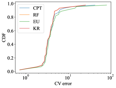
Figure 2. CDF of Cross-Validated Errors. (The CDFs for kernel regression and random forest overlap.)

To obtain simpler summary statistics for the comparison between the economic models and black boxes, we normalize each economic model’s error (in each domain) by the random forest error. Table 1 averages this ratio across domains and shows that on average, the cross-validated errors of the economic models are slightly larger than the random forest error: The CPT error is on average 1.06 times the random forest error, and the EU error is on average 1.21 times the random forest error.

Model	Normalized Error
EU	1.21
CPT variants
$\gamma$	1.12
$\alpha,\beta$	1.22
$\delta,\gamma$	1.08
$\alpha,\beta,\gamma$	1.07
$\alpha,\beta,\delta,\gamma$	1.06

Table 1. Average ratio of out-of-sample errors relative to random forest.

These results suggest that the different prediction methods we consider are comparable for within-domain prediction, with the black boxes performing slightly better. But the results do not distinguish whether the economic models and black boxes achieve similar out-of-sample errors by selecting approximately the same prediction rules, or if the rules they select lead to substantially different predictions out-of-domain. We also cannot determine whether the slightly better within-domain performance of the black box algorithms is achieved by learning generalizable structure that the economic models miss, or if the gains of the black boxes are confined to the domains on which they were trained. We next separate these explanations by evaluating the transfer performance of the models.

4.4. Transfer performance

We use the results in Section 3 to construct forecast intervals for transfer error, normalized transfer error, and transfer deterioration for each of the decision rules described above. In our meta-data there are $n=44$ domains, and we choose $r=1$ of these to use as the training domain. This choice of $r$ corresponds to the question, “If I draw one domain at random, and then try to generalize to another domain, how well do I do?”

Figure 3 displays two-sided forecast intervals for transfer error, normalized transfer error (where $R$ includes all decision rules shown in the figure), and transfer deterioration. These forecast intervals use $\tau=0.95$, so the upper bound of the forecast interval is the 95th percentile of the pooled transfer errors (across choices of the training and test domains), and the lower bound of the forecast interval is the 5th percentile of the pooled transfer errors. Applying Proposition 1, these are 81% forecast intervals. Choosing larger $\tau$ results in wider forecast intervals that have higher coverage levels, and we report some of these alternative forecast intervals in Online Appendix R.5, including a 91% forecast interval.

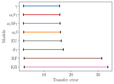
(a)

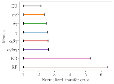
(b)

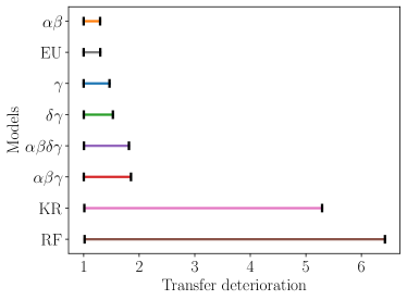
(c)

Figure 3. 81% (n=44, $\tau=0.95$) forecast intervals for (a) transfer error, (b) normalized transfer error (with $\mathcal{R}$ consisting of the decision rules shown in the figure), and (c) transfer deterioration.

Our main takeaway from Figure 3 is that although the prediction methods we consider are very similar from the perspective of within-domain prediction, they have very different out-of-domain implications.

Panel (a) of Figure 3 shows that the black box forecast intervals for transfer error have upper bounds that are roughly twice those of the economic models. For the normalized transfer error, which removes the common variation across models that emerges from variation in the predictability of the different target samples, the contrast between the economic models and the black boxes grows larger. Thus, although the economic models and the black box models select prediction rules that are close for the purposes of prediction in the training domain, they sometimes have very different performances in the test domain, and the prediction rules selected by the economic models generalize substantially better.

Panel (c) of Figure 3 shows an even starker contrast between the black boxes and economic models, which suggests that the value of retraining a black box on the target domain is quite high while it is less important to re-estimate the economic models. The ordering of the upper bounds of the forecast intervals is roughly consistent with the number of free parameters (with the exception of CPT($\alpha,\beta$), which has lower transfer deterioration than the single-parameter EU model and also CPT($\gamma$)).

All of the forecast intervals overlap for each of the three measures. This is not surprising, as variation in the transfer error due to the random selection of training and target domains cannot be eliminated even with data from many domains. We expect the black box intervals and the economic model intervals to overlap so long as the economic model errors on “upper tail” training and target domain pairs exceed the black box errors on “lower tail” training and target domain pairs. Section 5 provides confidence intervals for different population quantities, including quantiles of the transfer error distribution and the expected transfer error, whose width we do expect to vanish as the number of domains grow large. There, we find similar conclusions with regards to the relative performance of the black box algorithms and economic models.

The appendix provides several robustness checks and complementary analyses. Online Appendix R.5 plots the $\tau$-th percentile of pooled transfer errors as $\tau$ varies, demonstrating that forecast intervals constructed using other choices of $\tau$ (besides $\tau=0.95$) would look similar to those shown in the main text. Online Appendix R.6 provides 81% forecast intervals for the ratio of the CPT error to the random forest error, and finds that the random forest error is sometimes much higher than the CPT error, but is rarely much lower. Online Appendix R.7 considers an alternative choice for the number of training domains, setting $r=3$ instead of $r=1$. While the results are similar, the contrast between the economic models and black boxes is not as large, suggesting that the relative performance of the black boxes improves given a larger number of training domains. Online Appendix R.2 provides forecast intervals when each of the 14 papers is treated as a different domain; once again the black box methods transfer worse than the economic models do.

We next use our theoretical results from Section 3.2 to study the consequences of relaxing the iid assumption in our comparison of CPT$(\alpha,\beta,\delta,\gamma)$ and RF. Since the main differences observed above concerned the upper bounds of our forecast intervals, we limit attention to $\tau\geq 0.5,$ and compare the methods in terms of worst-case and everywhere upper-dominance with respect to all three measures of the transfer performance. These results are summarized in Table 2.

Type	transfer error	normalized transfer error	transfer deterioration
Worst-case dominance	$\tau\geq 0.5$	$\tau\geq 0.5$	$\tau\geq 0.5$
Everywhere dominance	$\tau\geq 0.954$	$\tau\geq 0.866$	$\tau\geq 0.647$

Table 2. Comparison between CPT and RF in terms of worst-case and everywhere upper-dominance. Each cell gives the range of $\tau$ at which CPT dominates RF.

Table 2 shows that CPT worst-case-upper-dominates RF at all quantiles $\tau\geq 0.5$ and for all three measures of transfer performance. Hence, our finding that the upper tail of transfer errors is larger for RF than for CPT is fully robust to relaxing the assumption that the training and test domains are drawn from the same distribution, provided that for a given degree of relaxation we are comfortable comparing the upper bound for one method to the upper bound for the other. In Appendix R.8, we provide a more detailed view of worst-case-upper-dominance by plotting $\bar{e}_{\tau}^{\mathbf{M}}(\Gamma)$ as functions of $\tau$ and $\Gamma$, respectively.

We can also consider the more demanding everywhere-upper-dominance criterion, which asks what happens if we relax our iid sampling assumption in a way which is as favorable to RF (and as unfavorable to CPT) as possible. We find a substantial degree of robustness even under this highly demanding criterion: CPT everywhere-upper-dominates RF in transfer error for all $\tau\geq 0.954,$ everywhere-dominates in normalized transfer error for $\tau\geq 0.866,$ and everywhere dominates in transfer deterioration for $\tau\geq 0.647.$

4.5. Do black boxes transfer poorly because they are too flexible?

One tempting explanation of our empirical findings is that because the black boxes are more flexible than the economic models, they can learn idiosyncratic details that do not generalize across subject pools, such as that some subject pools tend to value lotteries depending on specific digits they contain. This would lead the black boxes to have better within-domain prediction for those subject pools, but worse transfer performance if the regularity does not generalize across subject pools.

While the flexibility of black box algorithms is likely an important determinant of their transfer performance, there are at least two reasons this cannot be a complete explanation of our results. First, the flexibility gap between the black boxes and economic models is not large: many conditional mean functions (for binary lotteries) can be well approximated by CPT for some choice of parameters values $\alpha,\beta,\delta,\gamma$ (Fudenberg et al., 2021).

Second, black boxes do not always transfer worse. One of the papers we use is based on samples of certainty equivalents from 30 countries (l’Haridon and Vieider, 2019). Crucially, of the 30 samples from this paper, 29 samples report certainty equivalents for the same 27 lotteries, and the remaining sample reports certainty equivalents for 23 of those lotteries. We repeat our analysis using these 30 samples as the domains, and find that the forecast intervals for transfer error are indistinguishable across the prediction methods (Panel (a) of Figure 4). There is some separation between the forecast intervals for the remaining two measures, but in both cases the CPT and random forest forecast intervals are more similar than in the original data.

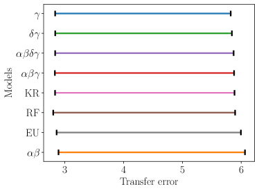
(a)

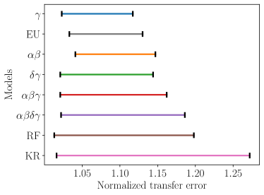
(b)

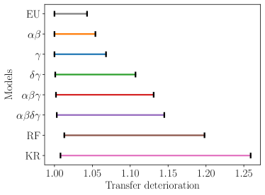
(c)

Figure 4. 78% (n=30, $\tau$=0.95) forecast intervals using samples in l’Haridon and Vieider (2019).

These observations show that flexible prediction methods do not always transfer poorly, although they do perform poorly in certain kinds of transfer prediction tasks. The next section explores one potential explanation.

4.6. Two kinds of transfer problems

Our framework allows the distribution $P$ governing the training sample and the distribution $P^{\prime}$ governing the test sample to differ. At one extreme, $P$ and $P^{\prime}$ may share a common marginal distribution on the feature space $\mathcal{X}$, but have very different conditional distributions $P_{Y\mid X}$ and $P^{\prime}_{Y\mid X}$ (known as model shift). In our application, this would mean that the distribution over lotteries is the same, but the conditional distribution of reported certainty equivalents is different across domains. At another extreme, the conditional distributions $P_{Y\mid X}$ and $P^{\prime}_{Y\mid X}$ might be the same, but the marginal distributions over the feature space could differ across domains, e.g., if different kinds of lotteries are used in different domains (known as covariate shift).

Our findings in Figure 4 suggest that black boxes do as well as economic models at transfer prediction when the primary source of variation across distributions is a shift in the conditional distribution, rather than a shift in the marginal distribution over features. Intuitively, the observed training data necessarily involves only a small part of the feature space (e.g., a specific set of lotteries). The black box algorithms and economic models both search through a class of prediction rules to find the one that best fits the observed data. In our application, this means finding a prediction rule that does a good job of predicting certainty equivalents for the lotteries in the training data. If the conditional distributions $P_{Y\mid X}$ governing the test and training samples are different, the best predictions in the training sample will not be the best predictions in the test sample. But economic models and black box algorithms are disadvantaged for transfer prediction in the same way.

In contrast, when the set of lotteries varies across samples, then transfer prediction necessarily involves extrapolation. If the economic model has identified structure that is shared across settings, then fixing its parameters at values selected to perform best on the training data will improve predictions for the test lotteries. This need not be true for an algorithm that hasn’t identified a structure that relates behavior across lotteries.

For a simple, stylized, example of this contrast, consider three domains with degenerate distributions over observations. In domain 1, the distribution is degenerate at the lottery $(z_{1},z_{2},p)=(10,0,1/2)$ and certainty equivalent $y=3$. In domain 2, the distribution is degenerate at the lottery $(z_{1},z_{2},p)=(10,0,1/2)$ and certainty equivalent $y=4$. In domain 3, the distribution is degenerate at a new lottery $(z_{1},z_{2},p)=(20,10,1/10)$ and certainty equivalent $y=11$. Suppose EU and a decision tree are both trained on a sample from domain 1. The CRRA parameter $\eta\approx 0.64$ perfectly fits the observation $(10,0,1/2;3)$, as does the trivial decision tree that predicts $y=3$ for all lotteries. The estimated EU model and decision tree are equivalent for predicting observations in domain 2: both predict $y=3$ and achieve a mean-squared error of $1$. But their errors are very different on domain 3: the EU prediction for the new lottery is approximately 10.8 with a mean-squared error of approximately 0.05, while the decision tree’s prediction is 3 with a mean-squared error of 64.

4.7. Predicting the relative transfer performance of black boxes and economic models

The preceding sections suggest that the relative transfer performance of black boxes and economic models is determined primarily by shifts in which lotteries are sampled, rather than shifts in behavior conditional on those lotteries. To further test this conjecture, we examine how well we can predict the ratio of the random forest transfer error to the CPT transfer error, $e(\rho^{RF}(\mathbf{M}_{\mathcal{T}}),S_{d})/e(\rho^{CPT}(\mathbf{M}_{\mathcal{T}}),S_{d})$, given information about the training and test lotteries but not about the distribution of certainty equivalents in either sample. If the relative performance of these methods depended importantly on behavioral shifts in the two domains—i.e., a change in the distribution of certainty equivalents for the same lotteries—then we would expect prediction of the relative performance based on lottery information alone to be poor. We find instead that lottery information has substantial predictive power for this ratio.

For each sample $S=\{(z_{1,i},z_{2,i},p_{i};y_{i})\}_{i=1}^{m}$, we consider the following features:

• the mean, standard deviation, max, and min value of $z_{1}$ among the lotteries in $S$

• the mean, standard deviation, max, and min value of $z_{2}$ among the lotteries in $S$

• the mean, standard deviation, max, and min value of $p$ among the lotteries in $S$

• the mean, standard deviation, max, and min value of $1-p$ among the lotteries in $S$

• the mean, standard deviation, max, and min of $pz_{1}+(1-p)z_{2}$ among the lotteries in $S$

• the size of $S$

• an indicator variable for whether $z_{1},z_{2}\geq 0$ for all lotteries in $S$

We consider three possible feature sets: (a) Training Only, which includes all features derived from the training sample $\mathbf{M}_{\mathcal{T}}$; (b) Test Only, which includes all features derived from the test sample $S_{d}$, (c) Both, which includes all features derived from the training sample $\mathbf{M}_{\mathcal{T}}$ and the test sample $S_{d}$. We evaluate two prediction methods: OLS and a random forest algorithm. Table 3 reports tenfold cross-validated errors for each of these feature sets and prediction methods. As a benchmark, we also consider the best possible constant prediction.

	Train Only	Test Only	Both
Constant	2.57	2.57	2.57
OLS	1.00	2.61	0.94
RF	0.98	2.52	0.76

Table 3. Cross-Validated MSE

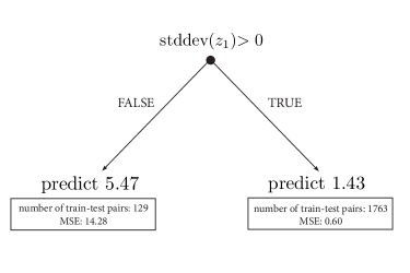
Figure 5. Best 1-split decision tree based on training and test features.

The best constant prediction achieves a mean-squared error of 2.57, which can be more than halved using features of the training set alone. Using features of both the training and test sets, the random forest algorithm reduces error to 30% of the constant model. Crucially, the random forest algorithm is permitted to learn nonlinear combinations of the input features, and thus discover relationships between the training and test lotteries that are relevant to the relative performance of the black box and the economic model.

The random forest algorithm is too opaque to deliver insight into how it achieves these better predictions, but we can obtain some understanding by examining the best 1-split decision tree, shown in Figure 5 below. This decision tree achieves a cross-validated MSE of 1.75, reducing the error of the constant model by 32%. It partitions the set of (train,test) domain pairs into two groups depending on whether the standard deviation of $z_{1}$ (the larger prize) in the training set of lotteries exceeds zero. There are three domains in which the prizes $(z_{1},z_{2})$ are held constant across all training lotteries (although the probabilities vary). In the 129 transfer prediction tasks where one of these three domains is used for training, the decision tree predicts the ratio of the random forest error to the CPT error to be 5.47. For all other transfer prediction tasks, the decision tree predicts 1.43.

This finding reinforces our intuition that the relative performance of the black boxes and economic models is driven in part by whether the training sample covers the relevant part of the feature space. When the training observations concentrate on an unrepresentative part of the feature space (such as all lotteries that share a common pair of prize outcomes), then the black boxes transfer much more poorly than economic models.

Our results also clarify a contrast between transfer performance and classical out-of-sample performance. In out-of-sample testing, the marginal distribution on $\mathcal{X}$ is the same for the training and test samples, so the set of training lotteries is likely to be representative of the set of test lotteries as long as the training sample is sufficiently large. When test and training samples are governed by distributions with different marginals on $\mathcal{X}$, the set of training lotteries can be unrepresentative of the set of test lotteries regardless of the number of training observations. Training on observations pooled across many domains alleviates the potential unrepresentativeness of the training data, but the number of domains needed will depend on properties of the distribution: An environment where each domain puts weight on exactly one lottery that is itself sampled iid may be difficult for black-box algorithms, while an environment where the marginal distribution is degenerate on the same lottery in all domains may be easier. There is no analog in out-of-sample testing for the role played by variation in the marginal distribution on $\mathcal{X}$ across domains. Moving beyond our specific application, we expect this variation to be an important determinant of the relative transfer performance of black box algorithms and economic models in general.

5. Extensions and further results

Our main results focus on forecasting realized transfer errors, which is useful when we want to know the range of plausible errors in transferring a given model to a new domain. We now complement those results with procedures for inference focused on population quantities: Section 5.2 provides confidence intervals for quantiles of the transfer error distribution, and Section 5.3 provides a confidence interval for the expected transfer error. Since these quantities can be perfectly recovered given data from an infinite number of domains, we expect the lengths of these intervals to vanish as the number of observed domains grows large, unlike the forecast intervals from Section 3.

5.1. Preliminary Lemma

We start by establishing a bound that will be useful in the subsequent construction of confidence intervals. Let

$$U=\frac{(n-k)!}{n!}\sum_{(i_{1},\dots,i_{k})\in\mathbb{T}_{r+1,n}}\phi(Z_{i_{1}},\dots,Z_{i_{k}})$$

be an arbitrary U-statistic of degree $k$ with a bounded (and potentially asymmetric) kernel $\phi$ that takes values in $[0,1]$.

Definition 1.

For every $n,k\in\mathbb{Z}_{+}$ and $x,y\in\mathbb{R}$, define

$$B_{n,k}(x;y)\equiv\min\Bigg{\{}b^{1}_{n,k}(x;y),b^{2}_{n,k}(x;y),b^{3}_{n,k}(x;y)\Bigg{\}}$$

where

$$b^{1}_{n,k}(x;y) \equiv\exp\left\{-\lceil n/k\rceil\left(x\wedge y\log\left(\frac{x\wedge y}{y}\right)+(1-x\wedge y)\log\left(\frac{1-x\wedge y}{1-y}\right)\right)\right\}$$

$$b^{2}_{n,k}(x;y) \equiv e\cdot\mathbb{P}\left({\rm Binom}(\lceil n/k\rceil;y)\leq\lceil\lceil n/k\rceil\cdot x\rceil\right)$$

$$b^{3}_{n,k}(x;y) \equiv\min_{\lambda>0}\frac{n\lambda}{k}\left(x-\frac{\lambda}{\lambda+kG(\lambda)}y\right)$$

Lemma 1.

If $\phi(Z_{1},\ldots,Z_{k})\in[0,1]$ almost surely, then $P(U\leq x)\leq B_{n,k}(x;\mathbb{E}(U))$ for every $x\in[0,1]$.

5.2. Quantiles of transfer error

Let $F$ denote the CDF of $e_{\mathbf{T},n+1}$, which we assume is continuous. This section builds a confidence interval for the $\beta$-th quantile of $F$, denoted $q_{\beta}$.

For arbitrary $q\in\mathbb{R}$ and realized metadata $\mathbf{M}=\{S_{1},\dots,S_{n}\}$, define

$$\varphi(q,\mathbf{M})=\frac{(n-r-1)!}{n!}\sum_{(d_{1},\ldots,d_{r+1})\in\mathbb{T}_{r+1,n}}\mathbb{I}(e_{(d_{1},\dots,d_{r}),d_{r+1}})\leq q)$$

where $\mathbb{I}(\cdot)$ is the indicator function, recalling that $e_{(d_{1},\dots,d_{r}),d_{r+1}}$ denotes the observed transfer error from samples $(S_{d_{1}},\dots,S_{d_{r}})$ to sample $S_{d_{r+1}}$. This is the fraction of observed transfer errors in the metadata (from $r$ training samples to one test sample) that are less than $q$. Then $U_{\beta}\equiv\varphi(q_{\beta},\mathbf{M})$ is a U-statistic where by definition, $\mathbb{E}[U_{\beta}]=\beta$. Lemma 1 then implies

$$\mathbb{P}(U_{\beta}\leq x)\leq B_{n,r+1}(x,\beta)\quad\quad\mathbb{P}(U_{\beta}\geq x)=\mathbb{P}(1-U_{\beta}\leq 1-x)\leq B_{n,r+1}(1-x,1-\beta).$$ (5.1)

Definition 2.

For any quantile $\beta\in(0,1)$ and confidence level $1-\alpha\in(0,1)$, let $\hat{u}^{+}_{\beta}(\alpha)=\inf\{u:B_{n,r+1}(u;\beta)\geq\alpha\}$ and $\hat{u}^{-}_{\beta}(\alpha)=\sup\{u:B_{n,r+1}(1-u;1-\beta)\geq\alpha\}$. Further define $\hat{q}_{\beta}^{\text{L}}(\alpha)\equiv\min\left\{q:\varphi(q,\mathbf{M})\geq\hat{u}^{+}_{\beta}(\alpha)\right\}$ and $\hat{q}_{\beta}^{\text{U}}(\alpha)\equiv\max\left\{q:\varphi(q,\mathbf{M})\leq\hat{u}^{-}_{r}(\alpha)\right\}.$

Since $B_{n,r+1}(u;\cdot)$ is right-continuous in $u$, it follows from (5.1) that $\mathbb{P}(U_{\beta}<\hat{u}^{+}_{\beta}(\alpha))\leq\alpha$ and $\mathbb{P}(U_{\beta}>\hat{u}^{-}_{\beta}(\alpha))\leq\alpha.$ Since $\varphi(q,\mathbf{M})$ is monotonically increasing in $q$, the event $\{U_{\beta}<\hat{u}^{+}_{\beta}(\alpha)\}$ is equivalent to $\{q_{\beta}<\hat{q}_{\beta}^{\text{L}}(\alpha)\}$, while $\{U_{\beta}>\hat{u}^{-}_{\beta}(\alpha)\}$ is equivalent to $\{q_{\beta}>\hat{q}_{\beta}^{\text{U}}(\alpha)\}.$ Thus we obtain:

Proposition 1.

For any quantile $\beta\in(0,1)$ and confidence level $1-\alpha\in(0,1)$,

$$\mathbb{P}(q_{\beta}\leq\hat{q}_{\beta}^{\text{U}}(\alpha))\geq 1-\alpha$$

and

$$\mathbb{P}\left(q_{\beta}\in\left[\hat{q}_{\beta}^{\text{L}}(\alpha/2),\hat{q}_{\beta}^{\text{U}}(\alpha/2)\right]\right)\geq 1-\alpha.$$

Figure 6 applies Proposition 1 to construct two-sided 81% confidence interval for the median transfer error, median normalized transfer error, and median transfer deterioration. As in Figure 3, these confidence intervals are substantially wider for the black box algorithms, and have higher upper bounds.

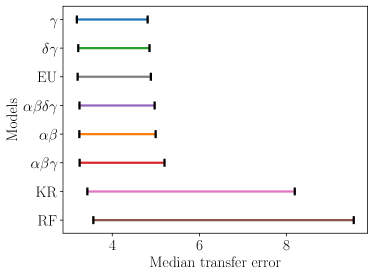
(a)

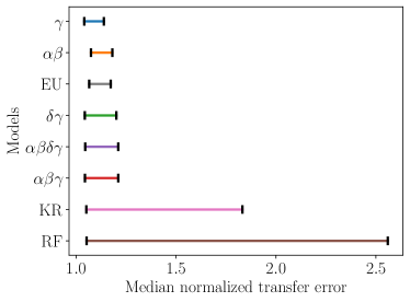
(b)

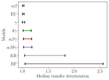
(c)

Figure 6. 81% confidence intervals for the median of (a) transfer error, (b) normalized transfer error, and (c) transfer deterioration.

5.3. Expected transfer error

This section constructs confidence intervals for the expected transfer error, $\mu\equiv\mathbb{E}(e_{\mathbf{T},n+1})$, under the assumption that transfer errors are uniformly bounded (in which case it is without loss to set $e_{\mathbf{T},n+1}\in[0,1]$). Define the U-statistic

$$U=\frac{(n-r-1)!}{n!}\sum_{(d_{1},\ldots,d_{r+1})\in\mathbb{T}_{r+1,n}}e_{(d_{1},\dots,d_{r}),d_{r+1}}.$$

Because $\mathbb{E}[U]=\mu$, Lemma 1 implies that $\mathbb{P}(U\leq x)\leq B_{n,r+1}(x,\mu)$ and $\mathbb{P}(U\geq x)\leq B_{n,r+1}(1-x,1-\mu)$ for all $x\in\mathbb{R}$.

Definition 3.

For any confidence guarantee $1-\alpha\in(0,1)$, let $\hat{\mu}^{+}(\alpha)=\sup\{\mu:B_{n,r+1}(U;\mu)\geq\alpha\}$ and $\hat{\mu}^{-}(\alpha)=\inf\{\mu:B_{n,r+1}(1-U;1-\mu)\geq\alpha\}$.

It follows from (5.1) that $\mathbb{P}(U<\hat{u}^{+}(\alpha))\leq\alpha$ and $\mathbb{P}(U>\hat{u}^{-}(\alpha))\leq\alpha$, which implies:

Proposition 2.

If $e_{T,d}\in[0,1]$ almost surely, then

$$\mathbb{P}\left(\mu\leq\hat{\mu}^{+}(\alpha)\right)\geq 1-\alpha$$

and

$$\mathbb{P}\left(\mu\in[\hat{\mu}^{-}(\alpha/2),\hat{\mu}^{+}(\alpha/2)]\right)\geq 1-\alpha.$$

Figure 7 applies this result to construct a two-sided 81% confidence intervals for our transferability measures. Since our main measures are not bounded, we report instead confidence intervals for the expectation of the inverse of normalized transfer error, i.e.,

$$\frac{\min_{\hat{\rho}\in\mathcal{R}}e(\hat{\rho}(S_{n+1}),S_{n+1})}{e(\rho(\mathbf{M}_{\mathbf{T}}),S_{n+1})}\in[0,1]$$

and the inverse of transfer deterioration, i.e.,

$$\frac{e(\rho(S_{n+1}),S_{n+1})}{e(\rho(\mathbf{M}_{\mathbf{T}}),S_{n+1})}\in[0,1].$$

Lower values for these measures correspond to worse transfer performance. We find again that the confidence intervals for the black box algorithms are qualitatively worse than those for the economic models.

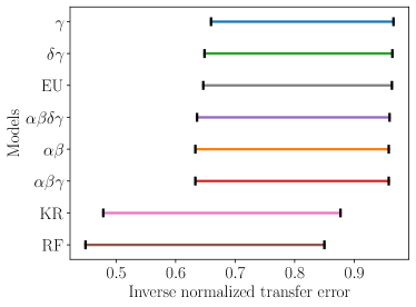
(a)

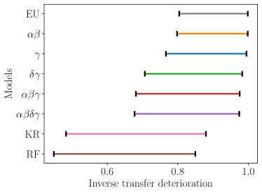
(b)

Figure 7. 81% forecast intervals for (a) expected inverse normalized transfer error, (b) expected inverse transfer deterioration.

6. Conclusion

Our measures of transfer error quantify how well a model’s performance on one domain extrapolates to other domains. We applied these measures to show that the predictions of expected utility theory and cumulative prospect theory outperform those of black box models on out-of-domain tests, even though the black boxes generally have lower out-of-sample prediction errors within a given domain. The relatively worse transfer performance of the black boxes seems to be because the black box algorithms have not identified structure that is commonly shared across domains, and thus cannot effectively extrapolate behavior from one set of features to another. Our finding that the economic models transfer better supports the intuition that economic models can recover regularities that are general across a variety of domains.

Appendix A Proofs

A.1. Notation

Throughout let $\mathcal{N}\equiv\{1,\dots,n\}$. The set $\mathbb{T}_{r,n}$ consists of all vectors of length $r$ with distinct values in $\mathcal{N}$. For any $(d_{1},\ldots,d_{r+1})\in\mathbb{T}_{r+1,n+1}$, let $f(d_{1},\ldots,d_{r+1})=e_{(d_{1},\dots,d_{r}),d_{r+1}}$ denote the transfer error from training samples $S_{d_{1}},\ldots,S_{d_{r}}$ to test sample $S_{d_{r+1}}$.

A.2. Proofs of Proposition 1 and Claim 1

Since $\mathbf{T}$ is a random subset of $\{1,\ldots,n\}$ that is independent of $\{S_{1},\ldots,S_{n+1}\}$,

$$\mathbb{P}\left(e_{\mathbf{T},n+1}\in A\right)=\mathbb{P}(e_{(1,\ldots,r),n+1}\in A)$$

for any event $A$ that is independent of $\mathbf{T}$. Thus, it suffices to prove Proposition 1 by replacing $\mathbf{T}$ with $(1,\ldots,r)$. We start by proving the one-sided guarantee:

$$\mathbb{P}\left(e_{(1,\ldots,r),n+1}\leq\bar{e}_{\tau}^{\mathbf{M}}\right)\geq\tau\left(1-\frac{r+1}{n+1}\right).$$

Throughout the proof we condition on the unordered samples $\{S_{1},\ldots,S_{n+1}\}$ and denote by $\{S_{(1)},\ldots,S_{(n+1)}\}$ any typical realization. Ranging over all possible choices of $r$ (ordered) training environments and a single test environment from $\{1,\ldots,n+1\}$ yields the multiset of transfer errors

$$\mathcal{C}=\bigg{\{}f(d_{1},\ldots,d_{r+1}):(d_{1},\ldots,d_{r+1})\in\mathbb{T}_{r+1,n+1}\bigg{\}},$$ (A.1)

which has size $(n+1)!/(n-r)!$. The subset of these transfer errors that don’t use sample $k$ for either training or testing is

$$\mathcal{C}_{-k}=\bigg{(}f(d_{1},\ldots,d_{r+1}):(d_{1},\ldots,d_{r+1})\in\mathbb{T}_{r+1,n+1},d_{j}\neq k,j=1,\ldots,r+1\bigg{)},$$

which has size $n!/(n-r-1)!$. For any $\tau\in[0,1]$, let $\bar{E}^{*}_{\tau}$ denote the $\lceil\tau n!/(n-r-1)!\rceil$-th smallest element in $\mathcal{C}$, and let $\bar{E}_{k,\tau}$ denote the $\lceil\tau n!/(n-r-1)!\rceil$-th smallest element in $\mathcal{C}_{-k}$. Since $\mathcal{C}_{-k}\subseteq\mathcal{C}$,

$$\bar{E}_{k,\tau}\geq\bar{E}^{*}_{\tau}\text{ for all $k$ and $\tau$.}$$ (A.2)

Let $\mathcal{F}$ denote the sigma-field generated by the unordered set $\{S_{(1)},\ldots,S_{(n+1)}\}$. Exchangeability implies that

$$\left(e_{(1,\ldots,r),n+1},\bar{e}_{\tau}\right)\mid\mathcal{F}\stackrel{{\scriptstyle d}}{{=}}\bigg{(}f(\bm{\pi}^{*}(1),\ldots,\bm{\pi}^{*}(r),\bm{\pi}^{*}(n+1)),\bar{E}_{\bm{\pi}^{*}(n+1),\tau}\bigg{)}$$

where $\bm{\pi}^{*}$ denotes a random permutation drawn from the uniform distribution over all permutations on $\{1,\ldots,n+1\}$. Thus

$$\mathbb{P}\left(e_{(1,\ldots,r),n+1}\leq\bar{e}_{\tau}\mid\mathcal{F}\right)=\mathbb{P}_{\bm{\pi}^{*}}\left(f(\bm{\pi}^{*}(1),\ldots,\bm{\pi}^{*}(r),\bm{\pi}^{*}(n+1))\leq\bar{E}_{\bm{\pi}^{*}(n+1),\tau}\right).$$ (A.3)

It follows that

$$\mathbb{P}\left(e_{(1,\ldots,r),n+1}\leq\bar{e}_{\tau}\mid\mathcal{F}\right) \geq\mathbb{P}_{\bm{\pi}^{*}}\left(f(\bm{\pi}^{*}(1),\ldots,\bm{\pi}^{*}(r),\bm{\pi}^{*}(n+1))\leq\bar{E}^{*}_{\tau}\right)$$ by (A.2) and (A.3)

$$=\frac{(n-r)!}{(n+1)!}\sum_{(d_{1},\ldots,d_{r+1})\in\mathbb{T}_{r+1,n+1}}\mathbb{I}(f(d_{1},\ldots,d_{r+1})\leq\bar{E}^{*}_{\tau})$$

$$=\frac{(n-r)!}{(n+1)!}\sum_{f\in\mathcal{C}}\mathbb{I}(f\leq\bar{E}^{*}_{\tau})$$

$$\geq\frac{(n-r)!}{(n+1)!}\left\lceil\tau\frac{n!}{(n-r-1)!}\right\rceil\geq\tau\left(1-\frac{r+1}{n+1}\right).$$

The one-sided guarantee then follows from the law of iterated expectation.

Turning to the two-sided guarantee, we first notice that the one-sided guarantee implies

$$\mathbb{P}\left(e_{(1,\ldots,r),n+1}>\bar{e}^{\mathbf{M}}_{\tau}\right)\leq 1-\tau+\tau\frac{r+1}{n+1},$$

and, by symmetry,

$$\mathbb{P}\left(e_{(1,\ldots,r),n+1}<\underline{e}^{\mathbf{M}}_{\tau}\right)\leq 1-\tau+\tau\frac{r+1}{n+1}.$$

Thus,

$$\mathbb{P}\left(e_{(1,\ldots,r),n+1}\in\left[\underline{e}^{\mathbf{M}}_{\tau},\bar{e}^{\mathbf{M}}_{\tau}\right]\right)\geq 2\tau-1-2\tau\frac{r+1}{n+1}.$$

This completes the proof of Proposition 1.

To prove Claim 1, define $\bar{E}^{\prime}_{\tau}$ to be the $\lfloor(1-\tau)n!/(n-r-1)!+1\rfloor$-th largest element in $\mathcal{C}$ as defined in (A.1). Since $|\mathcal{C}_{-k}|=n!/(n-r-1)!$, the quantity $\bar{E}_{k,\tau}$ is also the $\lfloor(1-\tau)n!/(n-r-1)!+1\rfloor$-th largest element in $\mathcal{C}_{-k}$. So $\bar{E}_{k,\tau}\leq\bar{E}^{\prime}_{\tau}$ for any $k$ and $\tau$.

$$\text{By \eqref{eq:pi_prob}, }\mathbb{P}\left(e_{(1,\ldots,r),n+1}\leq\bar{e}_{\tau}\mid\mathcal{F}\right) \leq\mathbb{P}_{\bm{\pi}^{*}}\left(f(\bm{\pi}^{*}(1),\ldots,\bm{\pi}^{*}(r),\bm{\pi}^{*}(n+1))\leq\bar{E}^{\prime}_{\tau}\right)$$

$$=\frac{(n-r)!}{(n+1)!}\sum_{(d_{1},\ldots,d_{r+1})\in\mathbb{T}_{r+1,n+1}}\mathbb{I}(f(d_{1},\ldots,d_{r+1})\leq\bar{E}^{\prime}_{\tau})$$

$$=\frac{(n-r)!}{(n+1)!}\sum_{f\in\mathcal{C}}\mathbb{I}(f\leq\bar{E}^{\prime}_{\tau}).$$

Claim 1 assumes that $\mathcal{C}$ has no ties almost surely, so $\sum_{f\in\mathcal{C}}\mathbb{I}(f>\bar{E}^{\prime}_{\tau})=\left\lfloor(1-\tau)\frac{n!}{(n-r-1)!}\right\rfloor.$ Thus

$$\mathbb{P}\left(e_{(1,\ldots,r),n+1}\leq\bar{e}_{\tau}\mid\mathcal{F}\right) \leq\frac{(n-r)!}{(n+1)!}\left(|\mathcal{C}|-\left\lfloor(1-\tau)\frac{n!}{(n-r-1)!}\right\rfloor\right)$$

$$\leq\frac{(n-r)!}{(n+1)!}\left(\frac{(n+1)!}{(n-r)!}-(1-\tau)\frac{n!}{(n-r-1)!}+1\right)$$

$$=\tau+(1-\tau)\frac{r+1}{n+1}+\frac{(n-r)!}{(n+1)!}.$$

The two-sided guarantee follows by symmetry.

A.3. Proof of Theorem 1

Again let $\mathcal{F}$ denote the sigma-field generated by the unordered set $\{S_{1},\ldots,S_{(n+1)}\}$. Under the assumed data-generating process,

$$e_{(d_{1},\ldots,d_{r}),n+1}\mid\mathcal{F}\stackrel{{\scriptstyle d}}{{=}}f(\bm{\pi}^{w}(d_{1}),\ldots,\bm{\pi}^{w}(d_{r}),\bm{\pi}^{w}(n+1)),\quad\forall(d_{1},\ldots,d_{r})\in\mathbb{T}_{r,n}.$$

where $\bm{\pi}^{w}$ is a random permutation on $\{1,\ldots,n+1\}$ distributed according to

$$\mathbb{P}(\bm{\pi}^{w}=\pi)=\frac{1}{n!}\frac{w(S_{\pi(n+1)})}{\sum_{j=1}^{n+1}\omega(S_{j})}.$$ (A.4)

On the other hand, $\mathbf{T}\stackrel{{\scriptstyle d}}{{=}}(\bm{\pi}^{n}(1),\ldots,\bm{\pi}^{n}(r))$ where $\bm{\pi}^{n}$ denotes a uniform random permutation on $\{1,\ldots,n\}$, so $e_{\mathbf{T},n+1}\mid\mathcal{F}\stackrel{{\scriptstyle d}}{{=}}f(\bm{\pi}^{w}\circ\bm{\pi}^{n}(1),\ldots,\bm{\pi}^{w}\circ\bm{\pi}^{n}(r),\bm{\pi}^{w}(n+1)).$ By (A.4), we have

$$e_{\mathbf{T},n+1}\mid\mathcal{F}\stackrel{{\scriptstyle d}}{{=}}f(\bm{\pi}^{w}(1),\ldots,\bm{\pi}^{w}(r),\bm{\pi}^{w}(n+1)).$$ (A.5)

For any $(d_{1},\ldots,d_{r},k)\in\mathbb{T}_{r+1,n+1}$,

$$\mathbb{P}((\bm{\pi}^{w}(1),\ldots,\bm{\pi}^{w}(r),\bm{\pi}^{w}(n+1))=(d_{1},\ldots,d_{r},k))=\frac{(n-r)!}{n!}\frac{w(S_{k})}{\sum_{j=1}^{n+1}\omega(S_{j})}\triangleq W_{k}^{\prime}.$$

Thus,

$$e_{\mathbf{T},n+1}\mid\mathcal{F}\sim\sum_{(d_{1},\ldots,d_{r},k)\in\mathbb{T}_{r+1,n+1}}W_{k}^{\prime}\cdot\delta_{f(d_{1},\ldots,d_{r},k)}.$$

Note that for any random variable $Z\sim F$, $\mathbb{P}(Z\leq\bar{Q}_{\tau}(F))\geq\tau$. Then

$$\mathbb{P}\left(e_{\mathbf{T},n+1}\leq\bar{Q}_{\tau}\left(\sum_{(d_{1},\ldots,d_{r},k)\in\mathbb{T}_{r+1,n+1}}W_{k}^{\prime}\cdot\delta_{f(d_{1},\ldots,d_{r},k)}\right)\mid\mathcal{F}\right)\geq\tau.$$ (A.6)

The value $f(d_{1},\ldots,d_{r},k)$ can be observed iff $d_{1},\ldots,d_{r},k$ are all not equal to $n+1$. The above unobserved upper confidence bound can be replaced by setting all unobserved $f$-values to $\infty$, i.e.,

$$\bar{Q}_{\tau}\left(\sum_{(d_{1},\ldots,d_{r},k)\in\mathbb{T}_{r+1,n}}W_{k}^{\prime}\cdot\delta_{f(d_{1},\ldots,d_{r},k)}+\Omega_{n+1}\cdot\delta_{\infty}\right).$$

where

$$\Omega_{n+1}=\sum_{(d_{1},\ldots,d_{r},k)\in\mathbb{T}_{r+1,n+1}\setminus\mathbb{T}_{r+1,n}}W_{k}^{\prime}.$$

Via a simple counting argument, we obtain that

$$\Omega_{n+1} =\frac{n!}{(n-r)!}W_{n+1}^{\prime}+\frac{r(n-1)!}{(n-r)!}\sum_{k=1}^{n}W_{k}^{\prime}$$

$$=\frac{r}{n}+\frac{(n-1)!}{(n-r-1)!}W_{n+1}^{\prime}$$

$$=\frac{r}{n}+\frac{n-r}{n}\frac{w(S_{n+1})}{\sum_{j=1}^{n+1}\omega(S_{j})}.$$ (A.7)

where the second to last equality uses $\sum_{k=1}^{n+1}W_{k}^{\prime}=\frac{(n-r)!}{n!}.$ By (A.7) and (3.5), we have $W_{k}=\frac{W_{k}^{\prime}}{1-\Omega_{n+1}},$ so

$$\bar{Q}_{\tau}\left(\sum_{(d_{1},\ldots,d_{r},k)\in\mathbb{T}_{r+1,n}}W_{k}^{\prime}\cdot\delta_{f(d_{1},\ldots,d_{r},k)}+\Omega_{n+1}\cdot\delta_{\infty}\right)$$

$$=\bar{Q}_{\frac{\tau}{1-\Omega_{n+1}}}\left(\sum_{(d_{1},\ldots,d_{r},k)\in\mathbb{T}_{r+1,n}}W_{k}\cdot\delta_{f(d_{1},\ldots,d_{r},k)}\right),$$

where the RHS is $\infty$ if $\tau\leq\Omega_{n+1}$.

Replacing $\tau$ by $\tau(1-\Omega_{n+1})$, (A.6) implies that

$$\mathbb{P}\left(e_{\mathbf{T},n+1}\leq\bar{Q}_{\tau}\left(\sum_{(d_{1},\ldots,d_{r},k)\in\mathbb{T}_{r+1,n}}W_{k}\cdot\delta_{f(d_{1},\ldots,d_{r},k)}\right)\mid\mathcal{F}\right)\geq\tau(1-\Omega_{n+1}).$$

The theorem now follows from the law of iterated expectation.

A.4. Proof of Lemma 1

Hoeffding (1963) shows that $P(U\leq x)\leq b^{1}_{n,k}(x,\mathbb{E}(U))$, and Bates et al. (2021) shows that $P(U\leq x)\leq b^{2}_{n,k}(x,\mathbb{E}(U))$. To show that if $x\in[0,1]$ then $P(U\leq x)\leq b^{3}_{n,k}(x,\mathbb{E}(U))$ we use a series of intermediate result to extend a result of Bates et al. (2021) on U-statistics of degree $2$ with bounded kernels to U-statistics with bounded kernels for any order $k\geq 2$.

Let $Z_{1},\ldots,Z_{n}$ be iid random variables and $\phi:\mathbb{R}^{k}\rightarrow[0,1]$ be a bounded function. Then a U-statistic of degree $k$ is defined as

$$U=\frac{(n-k)!}{n!}\sum_{i_{1},\ldots,i_{k}}\phi(Z_{i_{1}},\ldots,Z_{i_{k}}),$$ (A.8)

where $\sum_{i_{1},\ldots,i_{k}}$ denotes the sum over all $k$-tuples in $\mathcal{N}$ with mutually distinct elements. The average of $Z_{i}$ is a special case of (A.8) with $k=1$ and $\phi(z)=z$.

Let $m=\lfloor n/k\rfloor$ and $\bm{\pi}^{n}:\mathcal{N}\mapsto\mathcal{N}$ be a uniformly random permutation. For each permutation $\pi$, define

$$W_{\pi}=\frac{1}{m}\sum_{j=1}^{m}\phi\left(Z_{\pi((j-1)k+1)},\ldots,Z_{\pi(jk)}\right).$$

Note that the summands in $W_{\pi}$ are independent given $\pi$. Then $U=\mathbb{E}_{\bm{\pi}^{n}}[W_{\bm{\pi}^{n}}],$ where $\mathbb{E}_{\bm{\pi}^{n}}$ denotes the expectation with respect to $\bm{\pi}^{n}$ when conditioning on $Z_{1},\ldots,Z_{n}$. By Jensen’s inequality, for any convex function $\psi$, $\mathbb{E}[\psi(U)]=\mathbb{E}[\psi(\mathbb{E}_{\bm{\pi}^{n}}[W_{\bm{\pi}^{n}}])]\leq\mathbb{E}[\mathbb{E}_{\bm{\pi}^{n}}\psi(W_{\bm{\pi}^{n}})]=\mathbb{E}_{\bm{\pi}^{n}}[\mathbb{E}\psi(W_{\bm{\pi}^{n}})].$ Since $W_{\pi}$ has identical distributions for all $\pi$,

$$\mathbb{E}[\psi(U)]\leq\mathbb{E}[\psi(W_{\mathbf{id}})]$$ (A.9)

where $\mathbf{id}$ is the permutation that maps each element to itself.

Recalling that Hoeffding’s inequality is derived from the moment-generating function $\psi(z)=e^{\lambda z}$ (Hoeffding, 1963), and the Bentkus inequality is derived from the piecewise linear function $\psi(z)=(z-t)_{+}$ (Bentkus, 2004), the following tail inequalities for U-statistics are a direct consequence of (A.9).

Proposition 1.

Let $U$ be a U-statistic of order $k$ with a bounded kernel $\phi\in[0,1]$ in the form of (A.8) and $m=\lfloor n/k\rfloor$. Then

1. (Hoeffding inequality for U-statistics, Section 5 of Hoeffding 1963)

   $$\mathbb{P}(U\leq x)\leq\exp\left\{-mh_{1}\left(x\wedge\mathbb{E}[U];\mathbb{E}[U]\right)\right\},$$

   where

   $$h_{1}(y;\mu)=y\log\left(\frac{y}{\mu}\right)+(1-y)\log\left(\frac{1-y}{1-\mu}\right).$$

2. (Bentkus inequality for U-statistics, modified from Bentkus 2004)

   $$\mathbb{P}\left(U\leq x\right)\leq e\mathbb{P}\left(\mathrm{Bin}\left(m;\mathbb{E}[U]\right)\leq\lceil mx\rceil\right).$$

Other concentration inequalities can be derived from the leave-one-out property. Write $U(Z_{1},\ldots,Z_{n})$ for $U$ and let $U_{i}=\inf_{z_{i}}U(Z_{1},\ldots,Z_{i-1},z_{i},Z_{i+1},\ldots,Z_{n}).$ Note that $U_{i}$ is independent of $Z_{i}$. Since $\phi(\cdot)\geq 0$, we have $0\leq U-U_{i}\leq\frac{(n-k)!}{n!}\sum_{j=1}^{k}\sum_{i_{1},\ldots,i_{k},i_{j}=i}\phi(Z_{i_{1}},\ldots,Z_{i_{k}})$ so $\frac{n}{k}(U-U_{i})\leq 1$ and

$$\sum_{i=1}^{n}(U-U_{i})^{2} \leq\frac{((n-k)!)^{2}}{(n!)^{2}}\sum_{i=1}^{n}\left(\sum_{j=1}^{k}\sum_{i_{1},\ldots,i_{k},i_{j}=i}\phi(Z_{i_{1}},\ldots,Z_{i_{k}})\right)^{2}$$

$$\stackrel{{\scriptstyle(i)}}{{\leq}}\frac{k(n-k)!}{n\cdot n!}\sum_{j=1}^{k}\sum_{i=1}^{n}\sum_{i_{1},\ldots,i_{k},i_{j}=i}\phi(Z_{i_{1}},\ldots,Z_{i_{k}})^{2}$$

$$\stackrel{{\scriptstyle(ii)}}{{\leq}}\frac{k(n-k)!}{n\cdot n!}\sum_{j=1}^{k}\sum_{i=1}^{n}\sum_{i_{1},\ldots,i_{k},i_{j}=i}\phi(Z_{i_{1}},\ldots,Z_{i_{k}})$$

$$=\frac{k^{2}}{n}U,$$

where (i) applies the Cauchy-Schwarz inequality and (ii) uses the fact that $\phi(\cdot)\leq 1$. If we let $W=(n/k)U$ and $W_{i}=(n/k)U_{i}$, then $W-W_{i}\leq 1,\quad\sum_{i=1}^{n}(W-W_{i})^{2}\leq kW.$ This implies that $W$ as a function of $Z_{1},\ldots,Z_{n}$ satisfies the assumptions for the claim (34) in Theorem 13 of Maurer (2006) with constant $a=k$.

Proposition 2 (Theorem 13, Maurer 2006).

Let $G(\lambda)=(e^{\lambda}-\lambda-1)/\lambda$. Then for any $\lambda>0$,

$$\log\mathbb{E}[e^{\lambda(\mathbb{E}[W]-W)}]\leq\frac{k\lambda G(\lambda)}{\lambda+kG(\lambda)}\mathbb{E}[W].$$

This further implies that for any $x\in(0,\mathbb{E}[U])$,

$$\mathbb{P}\left(U\leq x\right)\leq\exp\left\{\min_{\lambda>0}\frac{n\lambda}{k}\left(x-\frac{\lambda}{\lambda+kG(\lambda)}\mathbb{E}[U]\right)\right\}.$$

Putting Proposition 1 and Proposition 2 together yields Lemma 1.

Online appendix to the paper

The Transfer Performance of Economic Models

Isaiah Andrews  Drew Fudenberg  Lihua Lei  Annie Liang  Chaofeng Wu

March 7, 2024

Appendix P Supplementary Material to Section 2

P.1. Other choices for $e_{\mathbf{T},d}$

Example 1 (Ratios of Model Errors).

For any two decision rules $\rho$ and $\rho^{\prime}$, set

$$e_{T,d}\equiv\frac{e(\rho(\mathbf{M}_{\mathcal{T}}),S_{d})}{e(\rho^{\prime}(\mathbf{M}_{\mathcal{T}}),S_{d})}$$

to be the ratio of the transfer errors of the two decision rules.

Example 2 (Partial Transfer).

Choose an economic model that can be represented as $\Sigma^{*}=\{\sigma_{\theta,\lambda}\}_{\theta\in\Theta,\lambda\in\Lambda}$ for compact sets $\Theta$ and $\Lambda$. The parameters in $\Lambda$ are domain-specific parameters that will be re-estimated on the target sample, while the parameters in $\Theta$ are transferred across domains. For any $\theta$ and sample $S$, define $e(\theta,S)=\min_{\lambda\in\Lambda}\frac{1}{|S|}\sum_{(x,y)\in S}\ell(\sigma_{\theta,\lambda}(x),y)$ to be the minimal achievable error on the sample $S$ when optimizing over $\lambda$ given the fixed value of $\theta$. The partial transfer error from $\mathbf{M}_{\mathcal{T}}$ to $S$ is $e(\theta_{\mathbf{M}_{\mathcal{T}}},S)$, where

$$\theta_{\mathbf{M}_{\mathcal{T}}}\in\operatorname*{argmin}_{\theta\in\Theta}\sum_{S\in\mathbf{M}_{\mathcal{T}}}\min_{\lambda\in\Lambda}e(\sigma_{\theta,\lambda},S)$$

is a best-fitting value of $\theta$ on the training data $\mathbf{M}_{\mathcal{T}}$. Set $e_{T,d}\equiv e(\theta_{\mathbf{M}_{\mathcal{T}}},S_{d})$ to be the partial transfer error on sample $S_{d}$.

P.2. Other decision rules

Example 3 (Domain Cross-Validation).

Let $\mathcal{R}^{*}$ be a family of decision rules, for example random forest algorithms with decision trees restricted to different depths. Let

$$\rho^{*}_{\mathbf{M}_{\mathcal{T}}}\in\operatorname*{argmin}_{\widetilde{\rho}\in\mathcal{R}^{*}}\sum_{t\in\mathcal{T}}e(\widetilde{\rho}(\mathbf{M}_{\mathcal{T}\setminus\{t\}}),S_{t})\quad\forall\mathbf{M}_{\mathcal{T}}\in\mathcal{M},|\mathcal{T}|\geq 2$$

and set $\rho(\mathbf{M}_{\mathcal{T}})=\rho^{*}(\mathbf{M}_{\mathcal{T}})$. That is, we pick the decision rule which, among the set of candidates $R^{*}$, attains the best average leave-one-domain-out error across our training domains, and then apply that rule to the full training data.

Example 4 (Distributionally Robust Optimization (DRO)).

DRO chooses model parameters to minimize worst-case error with respect to a neighborhood of distributions around the training data. Specify a distance function $D(P,P^{\prime})$ for the distance between any two probability measures $P,P^{\prime}\in\Delta(\mathcal{X}\times\mathcal{Y})$ and choose a neighborhood size $\varepsilon$. For any meta-data realization $\mathbf{M}_{\mathcal{T}}$, let $P_{\mathbf{M}_{\mathcal{T}}}$ denote the empirical distribution of the pooled set of observations across the samples in the meta-data. As in Example 1, consider a set of prediction rules $\Sigma^{*}$. We define $\rho_{\Sigma^{*}}$ to satisfy

$$\rho_{\Sigma^{*}}(\mathbf{M}_{\mathcal{T}})\in\operatorname*{argmin}_{\sigma\in\Sigma^{*}}\left(\max_{P\in B_{\varepsilon}\left(P_{\mathbf{M}_{\mathcal{T}}}\right)}\mathbb{E}_{P}[\ell(\sigma(x),y)]\right).$$

That is, the chosen prediction rule is the one that minimizes the worst-case error on distributions in the neighborhood of the observed data.

Example 5 (Hierarchical Bayesian Model).

A Hierarchical Bayesian model posits a parametric form for the data generating process in each domain $d,$ with parameters $\theta_{d}$ that can vary across domains. For instance, we might model the outcome $y$ as normally distributed conditional on the features $x,$ with conditional variance $\varsigma_{d}$ and conditional mean $\sigma_{\theta_{d}}(x)$, and specify a family of priors $\pi(\theta_{d},\varsigma_{d};\gamma)$ for the domain-level parameters $(\theta_{d},\varsigma_{d})$, as well as a prior $\pi(\gamma)$ on the hyperparameter $\gamma$ which is common across domains, and indexes the distribution of $(\theta_{d},\varsigma_{d})$. In this case the log-likelihood for the training data in domain $d$, fixing $\varsigma_{d}$ and varying $\theta_{d},$ is proportional to squared error loss. The hierarchical Bayes decision rule $\rho^{HB}(\mathbf{M}_{\mathcal{T}})$ for squared error loss then computes the posterior on $(\gamma,\{\theta_{d}:d\in T\})$ based on the training data $\mathbf{M}_{\mathcal{T}}$ and sets the prediction rule based on features $x$ in domain $d^{\prime}$ equal to the posterior mean of $\sigma_{\theta_{d^{\prime}}}(x).$

Appendix Q Supplementary Material to Section 3.2

Q.1. Algorithm for evaluating worst-case-upper-dominance

We provide an algorithm that computes $\bar{e}_{\tau}(\Gamma)$ with a single $\tau$ in $O(rn^{r+1}\log n)$ time and computes $\bar{e}_{\tau}(\Gamma)$ for all $\tau\in(0,1)$ in $O(rn^{r+1}\log n+n^{r+2})$ time. Recall the definition of $\mathcal{C}$ in (A.1). First, sort the elements in $\mathcal{C}$ as

$$f_{(1)}\leq f_{(2)}\leq\ldots\leq f_{(|\mathbb{T}_{r+1,n}|)},$$

where

$$f_{(j)}=f(d^{(j)}),\quad d^{(j)}=(d_{1}^{(j)},\ldots,d_{r+1}^{(j)})\in\mathbb{T}_{r+1,n}.$$

Let $\psi^{(j)}\in\{0,1\}^{n}$ with

$$\psi_{i}^{(j)}=I\left(d_{r+1}^{(j)}=i\right).$$

Further define the cumulative sum of $\psi^{(j)}$ as

$$\Psi^{(j)}=\sum_{\ell=1}^{j}\psi^{(\ell)}.$$

Let $w=(\omega(S_{1}),\ldots,\omega(S_{n}))^{T}$ and $\mathbf{1}_{n}=(1,1,\ldots,1)^{T}$. By (3.5), for each $j$,

$$f_{(j)}\geq\bar{e}_{\tau}^{\mathbf{M},\omega}\Longleftrightarrow\frac{(n-r-1)!}{(n-1)!}\frac{w^{T}\Psi^{(j)}}{w^{T}\mathbf{1}_{n}}\geq\tau.$$

Therefore,

$$\bar{e}_{\tau}^{\mathbf{M},\omega}=f_{J^{\omega}},\quad\text{where }J_{\tau}^{\omega}=\min\left\{j:\frac{w^{T}\Psi^{(j)}}{w^{T}\mathbf{1}_{n}}\geq\tau\frac{(n-1)!}{(n-r-1)!}\right\}.$$

By definition, the set of $w$ generated by all $\omega\in\mathcal{W}(\Gamma)$ is $[\Gamma^{-1},\Gamma]^{n}$. Thus,

$$\bar{e}_{\tau}^{\mathbf{M}}(\Gamma)=f_{J_{\tau}(\Gamma)},\quad\text{where }J_{\tau}(\Gamma)=\min\left\{j:\min_{w\in[\Gamma^{-1},\Gamma]^{n}}\frac{w^{T}\Psi^{(j)}}{w^{T}\mathbf{1}_{n}}\geq\tau\frac{(n-1)!}{(n-r-1)!}\right\}.$$ (Q.1)

Via some algebra, we can further simplify the expression of $\bar{e}_{\tau}^{\mathbf{M}}(\Gamma)$.

Theorem 1.

Let $\bar{\Psi}_{k}^{(j)}$ be the average of the $k$-smallest coordinates of $\Psi^{(j)}$ and

$$Q_{j}(\Gamma)=\frac{j}{n}+\min_{k\in\mathcal{N}}\frac{\bar{\Psi}_{k}^{(j)}-\frac{j}{n}}{1+\frac{n}{k(\Gamma^{2}-1)}}.$$

Then $Q_{j}(\Gamma)$ is strictly increasing in both $j$ and $\Gamma$. Moreover, $\bar{e}_{\tau}^{\mathbf{M}}(\Gamma)=f_{(J_{\tau}(\Gamma))}$, where

$$J_{\tau}(\Gamma)=\min\left\{j\geq\tau\frac{n!}{(n-r-1)!}:Q_{j}(\Gamma)\geq\tau\frac{(n-1)!}{(n-r-1)!}\right\}.$$

Proof.

First, we prove that

$$\min_{w\in[\Gamma^{-1},\Gamma]^{n}}\frac{w^{T}\Psi^{(j)}}{w^{T}\mathbf{1}_{n}}=\min_{w\in\{\Gamma^{-1},\Gamma\}^{n}}\frac{w^{T}\Psi^{(j)}}{w^{T}\mathbf{1}_{n}}.$$ (Q.2)

Let $g_{j}(w)=w^{T}\Psi^{(j)}/w^{T}\mathbf{1}_{n}$. Then $g_{j}$ is continuous and bounded on the closed set $[\Gamma^{-1},\Gamma]^{n}$ and thus the minimum can be achieved. Let

$$w^{(j)}(\Gamma)=\operatorname*{argmin}_{w:g_{j}(w)=\min_{w\in[\Gamma^{-1},\Gamma]^{n}}g_{j}(w)}\sum_{i=1}^{n}\min\left\{|w_{i}-\Gamma|,|w_{i}-\Gamma^{-1}|\right\}.$$

Suppose there exists $i\in\mathcal{N}$ such that $w_{i}^{(j)}(\Gamma)\in(\Gamma^{-1},\Gamma)$. Then

$$g_{j}(w_{i},w_{-i})=\frac{\Psi_{i}^{(j)}w_{i}+\Psi_{-i}^{(j)T}w_{-i}}{w_{i}+\mathbf{1}_{n-1}^{T}w_{-i}}=\Psi_{i}^{(j)}+\frac{\Psi_{-i}^{(j)T}w_{-i}-\Psi_{i}^{(j)}\cdot\mathbf{1}_{n-1}^{T}w_{-i}}{w_{i}+\mathbf{1}_{n-1}^{T}w_{-i}},$$

where $\Psi_{-i}^{(j)}$ and $w_{-i}$ are the leave-$i$-th-entry subvectors of $\Psi^{(j)}$ and $w$. Clearly, $g_{j}$ is a monotone function of $w_{i}$ for any given $w_{-i}$. Since $w^{(j)}(\Gamma)$ is a minimizer and $w_{i}^{(j)}(\Gamma)\in(\Gamma^{-1},\Gamma)$, we must have $\Psi_{-i}^{(j)T}w_{-i}-\Psi_{i}^{(j)}\cdot\mathbf{1}_{n-1}^{T}w_{-i}=0$. Define $\widetilde{w}^{(j)}(\Gamma)$ with

$$\widetilde{w}_{i}^{(j)}(\Gamma)=\Gamma,\quad\widetilde{w}_{-i}^{(j)}(\Gamma)=w_{-i}^{(j)}(\Gamma).$$

Then

$$g_{j}(\widetilde{w}^{(j)}(\Gamma))=g_{j}(w^{(j)}(\Gamma))=\min_{w\in[\Gamma^{-1},\Gamma]^{n}}g_{j}(w),$$

while

$$\sum_{i=1}^{n}\min\left\{|\widetilde{w}_{i}^{(j)}(\Gamma)-\Gamma|,|\widetilde{w}_{i}^{(j)}(\Gamma)-\Gamma^{-1}|\right\}<\sum_{i=1}^{n}\min\left\{|w_{i}^{(j)}(\Gamma)-\Gamma|,|w_{i}^{(j)}(\Gamma)-\Gamma^{-1}|\right\}.$$

This contradicts the definition of $w^{(j)}(\Gamma)$, so $w^{(j)}(\Gamma)\in\{\Gamma^{-1},\Gamma\}^{n},$ which completes the proof of (Q.2).

For any $w\in\{\Gamma^{-1},\Gamma\}^{n}$ with $|\{i:w_{i}=\Gamma\}|=k$, the Fréchet-Hoeffding inequality implies that $\Gamma$’s are allocated to the $k$ smallest entries of $\Psi^{(j)}$. Thus,

$$\min_{w\in\{\Gamma^{-1},\Gamma\}^{n}}\frac{w^{T}\Psi^{(j)}}{w^{T}\mathbf{1}_{n}}=\min_{k\in\mathcal{N}\cup\{0\}}\frac{\Gamma k\bar{\Psi}_{k}^{(j)}+\Gamma^{-1}(\mathbf{1}_{n}^{T}\Psi_{i}^{(j)}-k\bar{\Psi}_{k}^{(j)})}{\Gamma k+\Gamma^{-1}(n-k)}.$$

By definition, $\mathbf{1}_{n}^{T}\Psi_{i}^{(j)}=j$. Then for each $k$, the above expression can be simplified as

$$\frac{\Gamma k\bar{\Psi}_{k}^{(j)}+\Gamma^{-1}(\mathbf{1}_{n}^{T}\Psi_{i}^{(j)}-k\bar{\Psi}_{k}^{(j)})}{\Gamma k+\Gamma^{-1}(n-k)}=\frac{\Gamma k\bar{\Psi}_{k}^{(j)}+\Gamma^{-1}(j-k\bar{\Psi}_{k}^{(j)})}{\Gamma k+\Gamma^{-1}(n-k)}$$

$$=\frac{(\Gamma-\Gamma^{-1})k\bar{\Psi}_{k}^{(j)}+\Gamma^{-1}j}{(\Gamma-\Gamma^{-1})k+\Gamma^{-1}n}=\frac{j}{n}+\frac{(\Gamma-\Gamma^{-1})k\left(\bar{\Psi}_{k}^{(j)}-\frac{j}{n}\right)}{(\Gamma-\Gamma^{-1})k+\Gamma^{-1}n}$$

$$=\frac{j}{n}+\frac{\bar{\Psi}_{k}^{(j)}-\frac{j}{n}}{1+\frac{n}{k(\Gamma^{2}-1)}}.$$

The above expression is $j/n$ for both $k=n$ and $k=0$, so we can remove $0$ from the minimum, and thus

$$\min_{w\in[\Gamma^{-1},\Gamma]^{n}}\frac{w^{T}\Psi^{(j)}}{w^{T}\mathbf{1}_{n}}=Q_{j}(\Gamma).$$

By (Q.1),

$$\bar{e}_{\tau}^{\mathbf{M}}(\Gamma)=\min\left\{j:Q_{j}(\Gamma)\geq\tau\frac{(n-1)!}{(n-r-1)!}\right\}.$$

Finally, we can restrict to $j\geq\tau n!/(n-r-1)!$ because $Q_{j}(\Gamma)\leq\frac{j}{n}$ by taking $k=n$. ∎

Since $Q_{j}(\Gamma)$ is increasing in $j$, $J_{\tau}(\Gamma)$ can be found via binary search with iteration complexity $O(\log n^{r+1})=O(r\log n)$. Each iteration costs at most $O(n)$ operations to sort the entries of $\Psi^{(j)}$ based on the ordered version of $\Psi^{(j-1)}$, since there is only entry updated, and $O(n)$ additional operations to compute $Q_{j}(\Gamma)$. Thus, the overall computational overhead after obtaining $(f_{(1)},\ldots,f_{(|\mathbb{T}_{r+1,n}|)})$ is just $O(rn\log n)$, which is much smaller than the cost of sorting $f$-values $O(n^{r+1}\log n^{r+1})=O(rn^{r+1}\log n)$.

In some cases, we want to compute $\bar{e}_{\tau}^{\mathbf{M}}(\Gamma)$ for all $\tau\in[0,1]$ at once. The following result links $\bar{e}_{\tau}^{\mathbf{M}}(\Gamma)$ to an induced distribution on the $f$’s.

Corollary 1.

For any $\Gamma\geq 1$, let $\mu_{\Gamma}$ be a weighted measure with

$$\mu_{\Gamma}=\sum_{j=1}^{|\mathbb{T}_{r+1,n}|}\frac{(n-r-1)!}{(n-1)!}(Q_{j}(\Gamma)-Q_{j-1}(\Gamma))\cdot\delta_{f_{(j)}},$$

where $Q_{0}(\Gamma)=0$. Then $\bar{e}_{\tau}^{\mathbf{M}}(\Gamma)$ is the $\tau$-th quantile of $\mu_{\Gamma}$.

Since the ordering takes $O(rn^{r+1}\log n)$ time and computing each $Q_{j}(\Gamma)$ takes $O(n)$ time, the total computational cost to compute $\bar{e}_{\tau}^{\mathbf{M}}(\Gamma)$ for all $\tau\in[0,1]$ is $O(rn^{r+1}\log n+n^{r+2})$.

Q.2. Algorithm for evaluating everywhere dominance

Let $f_{(j),1}$ and $f_{(j),2}$ be the $j$-th largest transfer errors for method 1 and 2, respectively. Similarly, the count vectors for two methods are denoted by $\Psi^{(j),1}$ and $\Psi^{(j),2}$. Then method 1 does NOT everywhere-upper-dominate method 2 at the $\tau$-th quantile if and only if there exists $j_{1},j_{2}\in\{1,\ldots,|\mathbb{T}_{r+1,n}|\}$ and $W\in[0,\infty)^{n}$ such that

$$f_{(j_{1}),1}>f_{(j_{2}),2},\quad\frac{(n-r-1)!}{(n-1)!}\frac{w^{T}\Psi^{(j_{1}-1),1}}{w^{T}\mathbf{1}_{n}}<\tau\leq\frac{(n-r-1)!}{(n-1)!}\frac{w^{T}\Psi^{(j_{2}),2}}{w^{T}\mathbf{1}_{n}}.$$ (Q.3)

Above $\Psi^{(0),1}=(0,0,\ldots,0)^{T}$.

To avoid pairwise comparisons, which incur $O(n^{2(r+1)})$ computation, we can check (Q.3) by only focusing on $j_{1}=m(j),j_{2}=j$ where

$$m(j)=\min\{j^{\prime}:f_{(j^{\prime}),1}>f_{(j),2}\}.$$

It is easy to see that (Q.3) holds for some pair $(j_{1},j_{2})\in\{1,\ldots,|\mathbb{T}_{r+1,n}|\}^{2}$ if and only if it holds for $(m(j),j)$ for some $j\in\{1,\ldots,|\mathbb{T}_{r+1,n}|\}$. For any given $j$, (Q.3) reduces to

$$\frac{(n-r-1)!}{(n-1)!}\frac{w^{T}\Psi^{(m(j)-1),1}}{w^{T}\mathbf{1}_{n}}<\tau\leq\frac{(n-r-1)!}{(n-1)!}\frac{w^{T}\Psi^{(j),2}}{w^{T}\mathbf{1}_{n}},\quad w\in[0,\infty)^{n}.$$

This is equivalent to solving the following linear fractional programming problem and then checking if the objective is below $\tau$:

$$\min\frac{w^{T}a^{(j)}}{w^{T}\mathbf{1}_{n}},\quad\text{s.t., }\frac{w^{T}b^{(j)}}{w^{T}\mathbf{1}_{n}}\geq\tau,\quad w\in[0,\infty)^{n},$$

where

$$a^{(j)}=\Psi^{(m(j)),1}\cdot\frac{(n-r-1)!}{n-1)!},\quad b^{(j)}=\Psi^{(j),2}\cdot\frac{(n-r-1)!}{(n-1)!}.$$

We can apply the Charnes-Cooper transformation (Charnes and Cooper, 1962) by introducing $v=w/w^{T}\mathbf{1}_{n}$ to transform it into a linear programming problem:

$$\min v^{T}a^{(j)},\quad\text{s.t.,}\,\,v^{T}b^{(j)}\geq\tau,v^{T}\mathbf{1}_{n}=1,v\in[0,\infty)^{n}.$$ (Q.4)

Solving these $O(n^{r+1})$ LP problems can be accelerated by the following two observations:

1. Using the same argument as in the last step of the proof of Theorem 1, we can restrict

   $$j\geq\tau\frac{n!}{(n-r-1)!}.$$

2. When $a_{i}^{(j)}\geq b_{i}^{(j)}$ for every $i\in\mathcal{N}$, then the objective of (Q.4) can never be below $\tau$.

Appendix R Supplementary material for Section 4

R.1. Description of data

We briefly describe the individual samples in our meta-data. There are 44 domains in total.

Source of Data	# Obs	# Subj	# Lottery	Country	Gains Only
Abdellaoui et al. (2015)	801	89	3	France	Y
Fan et al. (2019)	4750	125	19	US	Y
Bouchouicha and Vieider (2017)	3162	94	66	UK	N
Sutter et al. (2013)	661	661	4	Austria	Y
Etchart-Vincent and l’Haridon (2011)	3036	46	20	France	N
Fehr-Duda et al. (2010)	8560	153	56	China	N
Lefebvre et al. (2010)	72	72	2	France	Y
Halevy (2007)	366	122	2	Canada	Y
Anderhub et al. (2001)	183	61	1	Israel	Y
Murad et al. (2016)	2131	86	25	UK	Y
Dean and Ortoleva (2019)	1032	179	3	US	Y
Bernheim and Sprenger (2020)	1071	153	7	US	Y
Bruhin et al. (2010)	8906	179	50	Switzerland	N
Bruhin et al. (2010)	4669	118	40	Switzerland	N
l’Haridon and Vieider (2019)	1708	61	27	Australia	N
l’Haridon and Vieider (2019)	2548	95	27	Belgium	N
l’Haridon and Vieider (2019)	2350	84	27	Brazil	N
l’Haridon and Vieider (2019)	2240	80	27	Cambodia	N
l’Haridon and Vieider (2019)	2687	96	27	Chile	N
l’Haridon and Vieider (2019)	5711	204	27	China	N
l’Haridon and Vieider (2019)	3072	128	23	Colombia	N
l’Haridon and Vieider (2019)	2968	106	27	Costa Rica	N
l’Haridon and Vieider (2019)	2770	99	27	Czech Republic	N
l’Haridon and Vieider (2019)	3906	140	27	Ethiopia	N
l’Haridon and Vieider (2019)	2604	93	27	France	N
l’Haridon and Vieider (2019)	3639	130	27	Germany	N
l’Haridon and Vieider (2019)	2352	84	27	Guatemala	N
l’Haridon and Vieider (2019)	2492	89	27	India	N
l’Haridon and Vieider (2019)	2352	84	27	Japan	N
l’Haridon and Vieider (2019)	2716	97	27	Kyrgyzstan	N
l’Haridon and Vieider (2019)	1791	64	27	Malaysia	N
l’Haridon and Vieider (2019)	3360	120	27	Nicaragua	N
l’Haridon and Vieider (2019)	5638	202	27	Nigeria	N
l’Haridon and Vieider (2019)	2660	95	27	Peru	N
l’Haridon and Vieider (2019)	2491	89	27	Poland	N
l’Haridon and Vieider (2019)	1959	70	27	Russia	N
l’Haridon and Vieider (2019)	1819	65	27	Saudi Arabia	N
l’Haridon and Vieider (2019)	1988	71	27	South Africa	N
l’Haridon and Vieider (2019)	2240	80	27	Spain	N
l’Haridon and Vieider (2019)	2212	79	27	Thailand	N
l’Haridon and Vieider (2019)	2070	74	27	Tunisia	N
l’Haridon and Vieider (2019)	2240	80	27	UK	N
l’Haridon and Vieider (2019)	2701	97	27	US	N
l’Haridon and Vieider (2019)	2436	87	27	Vietnam	N

R.2. Papers as domains

We now consider an alternative definition of domains, with each of the 14 papers representing a different domain. This changes the content of the iid assumption imposed in Section 3, where we now assume that samples are iid across papers, but may be dependent across subject pools within the same paper. We repeat our main analysis and report 65% two-sided forecast intervals in Figure 8. These intervals are qualitatively similar to those reported in Figure 3.

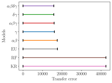
(a) Transfer error

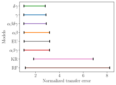
(b) Normalized transfer error

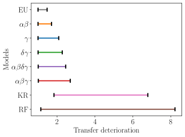
(c) Transfer deterioration

Figure 8. 65% (n=14, $\tau=0.95$) forecast intervals for each of the three measures, treating each paper as a separate domain.

R.3. In-sample errors

Figure 9 displays the CDFs of the in-sample errors of EU, CPT, the random forest algorithm, and kernel regression. As in Figure 2 (which reported out-of-sample errors), these curves are nearly indistinguishable.

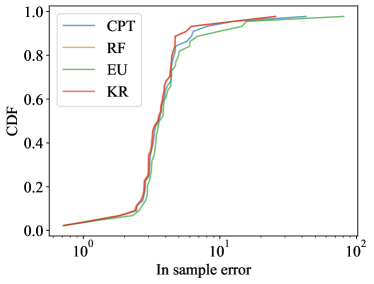
Figure 9. CDF of in-sample errors

R.4. Supplementary tables and figures for main analysis

Table 5 reports the forecast intervals that are depicted in Figure 3.

Model	Transfer Error	Normalized Error	Deterioration
CPT variants
$\gamma$	[2.50,15.83]	[1.03,2.54]	[1.00,1.47]
$\alpha,\beta$	[2.56,16.13]	[1.04,2.35]	[1.00,1.30]
$\delta,\gamma$	[2.48,17.19]	[1.02,2.47]	[1.00,1.53]
$\alpha,\beta,\gamma$	[2.47,15.91]	[1.02,2.60]	[1.00,1.85]
$\alpha,\beta,\delta,\gamma$	[2.46,15.99]	[1.02,2.62]	[1.00,1.82]
EU models
EU	[2.56,16.41]	[1.04,2.14]	[1.00,1.30]
ML algorithms
Random Forest	[2.71,31.39]	[1.02,6.42]	[1.02,6.42]
Kernel Regression	[2.75,33.62]	[1.02,5.33]	[1.01,5.29]

Table 5. 81% (n=44, $\tau=0.95$) forecast intervals

R.5. Alternative forecast intervals

In this section, we report alternative forecast intervals for our three measures. Table 6 constructs 91% two-sided forecast intervals (setting $\tau=1$), and Table 7 reports 91% one-sided forecast intervals (setting $\tau=0.95$). All of the forecast intervals are qualitatively similar to the 81% two-sided forecast intervals reported in the main text.

Model	Transfer Error	Normalized Error	Deterioration
CPT main variants
$\gamma$	[0.81,23104.96]	[1.01,7.31]	[1.00,7.22]
$\alpha,\beta$	[0.71,19999.41]	[1.00,5.28]	[1.00,5.27]
$\delta,\gamma$	[0.71,23052.76]	[1.00,7.25]	[1.00,7.18]
$\alpha,\beta,\gamma$	[0.71,28122.26]	[1.00,5.65]	[1.00,5.60]
$\alpha,\beta,\delta,\gamma$	[0.71,27959.10]	[1.00,6.01]	[1.00,5.95]
EU models
EU	[0.72,22787.99]	[1.00,4.44]	[1.00,1.75]
ML algorithms
Random Forest	[0.96,42520.49]	[1.01,33.17]	[1.01,33.17]
Kernel Regression	[1.01,42519.23]	[1.01,6.835]	[1.00,6.79]

Table 6. 91% (n=44, $\tau=1$) two-sided forecast intervals

Model	Transfer Error	Normalized Error	Deterioration
CPT main variants
$\gamma$	[0,15.83]	[1,2.54]	[1,1.47]
$\alpha,\beta$	[0,16.13]	[1,2.35]	[1,1.30]
$\delta,\gamma$	[0,17.19]	[1,2.47]	[1,1.53]
$\alpha,\beta,\gamma$	[0,15.91]	[1,2.60]	[1,1.85]
$\alpha,\beta,\delta,\gamma$	[0,15.99]	[1,2.62]	[1,1.82]
EU models
EU	[0,16.41]	[1,2.14]	[1,1.30]
ML algorithms
Random Forest	[0,31.39]	[1,6.42]	[1,6.42]
Kernel Regression	[0,33.62]	[1,5.33]	[1,5.29]

Table 7. 91% (n=44, $\tau=0.95$) one-sided forecast intervals

Finally, Figure 10 plots the $\tau$-th percentile of the pooled transfer errors as $\tau$ varies. The figure shows that the qualitative conclusions we have drawn about the relative performance of black boxes and economic models are not specific to any choice of $\tau$. In fact, in Panels (a) and (c), the black box curves lie everywhere above the CPT and EU curves, so both the lower and upper bounds of the black boxes’ forecast intervals are higher than those of the economic models for every choice of $\tau$.

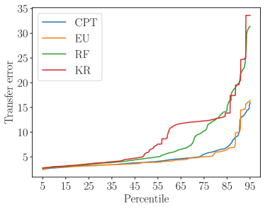
(a) Transfer error

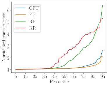
(b) Normalized transfer error

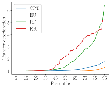
(c) Transfer deterioration

Figure 10. Error percentiles from 5 to 95 (truncated for readability).

R.6. Forecast intervals for the ratio of CPT and RF errors

Let $\rho^{CPT}$ denote the decision rule corresponding to CPT, and $\rho^{RF}$ denote the decision rule corresponding to the random forest algorithm. Define

$$e_{\mathcal{T},d}=\frac{e(\rho^{RF}(\mathbb{M}_{\mathcal{T}}),S_{d})}{e(\rho^{CPT}(\mathbb{M}_{\mathcal{T}}),S_{d})}$$

to be the ratio of the random forest transfer error to the CPT transfer error, henceforth the transfer error ratio.

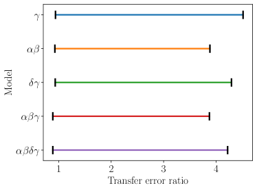
(a) 81% (n=44, $\tau=0.95$) Forecast intervals

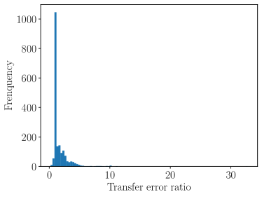
(b) Density

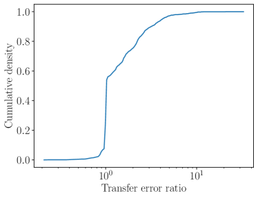
(c) CDF

Figure 11. Forecast intervals, density, and cdf for the ratio of the random forest transfer error to the CPT transfer error.

Panel (a) of Figure 11 reports 81% two-sided forecast intervals for the transfer error ratio for each CPT specification. The lower bound for each CPT model is approximately $0.9$, while the upper bound is as large as 4.5. Panel (b) of the figure is a histogram of transfer error ratios for the 4-parameter CPT model when the training domains $\mathcal{T}$ and the target domains $d$ are drawn uniformly at random from the set of domains in the meta-data. This distribution has a large cluster of ratios around 1 (i.e., CPT transfer errors are similar to the random forest errors) and a long right tail of ratios achieving a max value of 32.8 (i.e., the random forest error can be up to 32 times as large as the CPT error). The cumulative distribution function of $e_{T,d}$, reported in Panel (c) of Figure 11, shows that the random forest algorithm outperforms CPT in approximately $35\%$ of $(T,d)$ pairs, although CPT rarely has a much worse transfer error than the random forest and is sometimes much better.

R.7. Alternative Choice of $r$

Here we consider an alternative choice for the number of training domains, setting $r=3$ instead of $r=1$.

This corresponds to randomly choosing 3 of the 44 domains to be the training domains, finding the best prediction rule for this pooled data, and using the estimated prediction rule to predict the remaining 41 samples. For this analysis we use domain cross-validation to select tuning parameters for the black box algorithms, as described in Example 3.

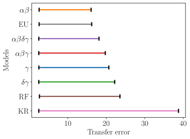
(a)

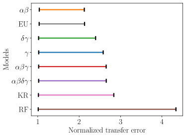
(b)

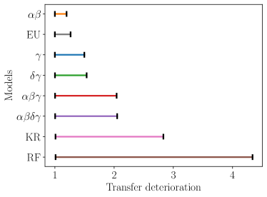
(c)

Figure 12. 73% (n=44, $\tau=0.95$) forecast intervals for (a) transfer error, (b) normalized transfer error, and (c) transfer deterioration, with the choice of $r=3$.

Figure 12 is the analog of Figure 3. Again we choose $\tau=0.95$, thus constructing forecast intervals whose lower bounds are the 5% percentile of pooled transfer errors, and whose upper bounds are the 95% percentile of pooled transfer errors. Applying Proposition 1, these are 73% forecast intervals. The most notable change is that the random forest forecast interval shrinks considerably, which suggests that the transfer error of the random forest algorithm becomes less variable when it is trained on more domains. Otherwise, all of the qualitative statements in the main text for $r=1$ continue to hold. In particular, as with $r=1$, we find that the forecast intervals for all three of our measures have higher lower and upper bounds for the black box algorithms than for the CPT specifications.

R.8. More details on worst-case dominance

Figures 13 and 14 compare the worst case upper bound of the forecast intervals for CPT and RF for our three transfer measures as either $\gamma$ or $\tau$ varies. In each case the dominance relation is clear.

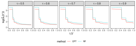
(a)

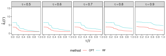
(b)

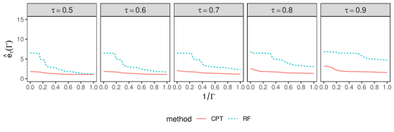
(c)

Figure 13. The worst case upper prediction bound $\hat{e}_{\tau}(\Gamma)$ (as defined in (3.6)) for (a) transfer errors, (b) normalized transfer errors, and (c) transfer deterioration of CPT and RF as a function of $\Gamma\in[1,\infty)$, discretized at $100/i(i=0,1,\ldots,100)$, at different quantiles $\tau\in\{0.5,0.6,0.7,0.8,0.9\}$.

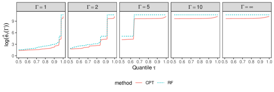
(a)

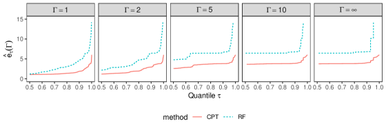
(b)

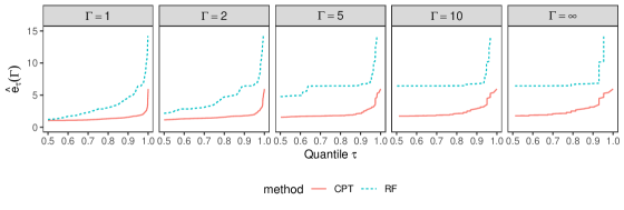
(c)

Figure 14. The worst case upper prediction bound $\hat{e}_{\tau}(\Gamma)$ (as defined in (3.6)) for (a) transfer errors, (b) normalized transfer errors, and (c) transfer deterioration of CPT and RF as a function of $\tau\in[0.5,1]$ without discretization for $\Gamma\in\{1,2,5,10,\infty\}$.

References

- Abdellaoui et al. (2015) Abdellaoui, M., P. Klibanoff, and L. Placido (2015): “Experiments on compound risk in relation to simple risk and to ambiguity,” Management Science, 61, 1306–1322.
- Agrawal et al. (2020) Agrawal, M., J. C. Peterson, and T. L. Griffiths (2020): “Scaling up psychology via Scientific Regret Minimization,” Proceedings of the National Academy of Sciences, 117, 8825–8835.
- Al-Ubaydli and List (2015) Al-Ubaydli, O. and J. A. List (2015): “420On the Generalizability of Experimental Results in Economics,” in Handbook of Experimental Economic Methodology, Oxford University Press.
- Allcott (2015) Allcott, H. (2015): “Site Selection Bias in Program Evaluation,” Quarterly Journal of Economics, 130, 1117–1165.
- Anderhub et al. (2001) Anderhub, V., W. Güth, Gneezy, and Sonsino (2001): “On the interaction of risk and time preferences: An experimental study,” German Economic Review, 2, 239–253.
- Andrews and Oster (2019) Andrews, I. and E. Oster (2019): “A simple approximation for evaluating external validity bias,” Economics Letters, 178, 58–62.
- Angelopoulos et al. (2022) Angelopoulos, A. N., S. Bates, A. Fisch, L. Lei, and T. Schuster (2022): “Conformal risk control,” arXiv preprint arXiv:2208.02814.
- Angrist and Fernández-Val (2013) Angrist, J. D. and I. Fernández-Val (2013): ExtrapoLATE-ing: External Validity and Overidentification in the LATE Framework, Cambridge University Press, vol. 3 of Econometric Society Monographs, 401–434.
- Aronow and Lee (2013) Aronow, P. M. and D. K. Lee (2013): “Interval estimation of population means under unknown but bounded probabilities of sample selection,” Biometrika, 100, 235–240.
- Athey (2017) Athey, S. (2017): “Beyond prediction: Using big data for policy problems,” Science, 355, 483–485.
- Athey and Imbens (2016) Athey, S. and G. Imbens (2016): “Recursive partitioning for heterogeneous causal effects,” Proceedings of the National Academy of Sciences, 113, 7353–7360.
- Bandiera et al. (2021) Bandiera, O., G. Fischer, A. Prat, and E. Ytsma (2021): “Do Women Respond Less to Performance Pay? Building Evidence from Multiple Experiments,” American Economic Review: Insights, 3, 435–54.
- Barber et al. (2021) Barber, R. F., E. J. Candes, A. Ramdas, and R. J. Tibshirani (2021): “Predictive inference with the jackknife+,” The Annals of Statistics, 49, 486–507.
- Bates et al. (2021) Bates, S., A. Angelopoulos, L. Lei, J. Malik, and M. Jordan (2021): “Distribution-free, risk-controlling prediction sets,” Journal of the ACM (JACM), 68, 1–34.
- Benartzi et al. (2017) Benartzi, S., J. Beshears, K. L. Milkman, C. R. Sunstein, R. H. Thaler, M. Shankar, W. Tucker-Ray, W. J. Congdon, and S. Galing (2017): “Should Governments Invest More in Nudging?” Psychological Science, 28, 1041–1055, pMID: 28581899.
- Bentkus (2004) Bentkus, V. (2004): “On Hoeffding’s inequalities,” The Annals of Probability, 32, 1650–1673.