SDSS J1042-0018 a broad line AGN but mis-classified as a HII galaxy in the BPT diagram by flux ratios of narrow emission lines

Abstract

In the manuscript, we discuss properties of the SDSS J1042-0018  which is a broad line AGN but mis-classified as a HII galaxy in the BPT diagram (SDSS J1042-0018  called as a mis-classified broad line AGN). The emission lines around H$\alpha$ and around H$\beta$ are well described by different model functions, considering broad Balmer lines to be described by Gaussian or Lorentz functions. Different model functions lead to different determined narrow emission line fluxes, but the different narrow emission line flux ratios lead the SDSS J1042-0018  as a HII galaxy in the BPT diagram. In order to explain the unique properties of the mis-classified broad line AGN SDSS J1042-0018, two methods are proposed, the starforming contributions and the compressed NLRs with high electron densities near to critical densities of forbidden emission lines. Fortunately, the strong starforming contributions can be preferred in the SDSS J1042-0018. The mis-classified broad line AGN SDSS J1042-0018, well explained by starforming contributions, could provide further clues on the applications of BPT diagrams to the normal broad line AGN.

1 Introduction

SDSS J1042-0018  (=SDSS J104210.03-001814.7) is a common broad line AGN with apparent broad emission lines, as the shown spectra in Fig. 1 from SDSS (Sloan Digital Sky Survey). However, based on flux ratios of narrow emission lines well discussed in Section 2, SDSS J1042-0018  can be well classified as a HII galaxy in the BPT diagram (Baldwin, Phillips & Terlevich 1981; Kewley et al. 2001; Kauffmann et al. 2003; Kewley et al. 2006, 2013a, 2019; Zhang et al. 2020). Therefore, in the manuscript, some special properties of SDSS J1042-0018  is studied and discussed.

Under the commonly accepted and well-known constantly being revised Unified Model (Antouncci 1993; Ramos et al. 2011; Netzer 2015; Audibert et al. 2017; Balokovic et al. 2018; Brown et al. 2019; Kuraszkiewicz et al. 2021), Type-1 AGN (broad line Active Galactic Nuclei) and Type-2 AGN (narrow line AGN) having the similar properties of intrinsic broad and narrow emission lines, however, Type-2 AGN have their central broad line regions (BLRs) with distances of tens to hundreds of light-days (Kaspi et al. 2000, 2005; Bentz et al. 2006, 2009; Denney et al. 2010; Bentz et al. 2013; Fausnaugh et al. 2017) to central black holes (BHs) totally obscured by central dust torus (or other high density dust clouds), leading to no broad emission lines (especially in optical band) in observed spectra of Type-2 AGN. Meanwhile, Type-1 AGN and Type-2 AGN have the similar properties of narrow emission lines, due to much extended narrow emission line regions (NLRs) with distances of hundreds to thousands of pcs (parsecs) to central BHs (Zakamska et al. 2003; Fischer et al. 2013; Hainline et al. 2014; Heckman & Best 2014; Fischer et al. 2017; Sun et al. 2017; Zhang & Feng 2017).

For an emission line object, two main methods can be conveniently applied to classify whether the object is an AGN or not? On the one hand, an broad line object with clear spectroscopic features of broad emission lines and the strong blue power-low continuum emissions can be directly classified as a type-1 AGN. On the other hand, for a narrow line object, the well-known BPT diagrams can be conveniently applied to determine which narrow line object is a Type-2 AGN (narrow line AGN) or a HII galaxy by properties of flux ratios of narrow emission lines. Therefore, the flux ratios of narrow emission lines for broad line objects (type-1 AGN) can also lead to the objects well classified as AGNs in the BPT diagrams. However, there are some special bright type-1 AGNs (we called them as the mis-classified AGNs), of which flux ratios of narrow emission lines lead the AGNs lying in the regions for HII galaxies in the BPT diagrams. More recently, Zhang (2021c) have reported the well identified quasar SDSS J1451+2709 as a mis-classified quasar, due to its mis-classification as a HII galaxy in the BPT diagrams through narrow emission line flux ratios, after considering different model functions applied to describe the emission lines. In the manuscript, the second mis-classified broad line AGN SDSS J1042-0018  is reported and discussed.

As discussed in Zhang (2021c), Type-1 AGN have more complicated line profiles of emission lines which will be discussed by different model functions leading to quite different properties of narrow emission lines. As the shown results in SDSS J1451+2709 in Zhang (2021c), there are intemediate broad emission lines have line width (second moment) around several hundreds of kilometers per second, gently wider than extended components of narrow emission lines, such as the commonly known extended components in [O iii]$\lambda 4950,5007$Å  doublet discussed in Greene & Ho (2005); Shen et al. (2011); Zhang & Feng (2017); Zhang (2021a, b). Once there are multi-epoch spectra, variability properties of emission components can be applied to determine whether one emission component is from NLRs. In the manuscript, although there is only single-epoch spectrum of SDSS J1042-0018, flux ratios of narrow emission lines can be applied to determine the classifications of SDSS J1042-0018  in the BPT diagram. In the manuscript, among the SDSS pipeline classified low-redshift quasars ($z~{}<~{}0.3$) (Richards et al. 2002; Ross et al. 2012), SDSS J1042-0018  is collected as the target, because the SDSS J1042-0018  is the second mis-classified broad line AGN as well discussed in the following sections, and further due to its clean line profiles of [O iii] doublet without extended components. The manuscript is organized as follows. Section 2 shows the properties of the spectroscopic emission lines by different model functions with different considerations. Section 3 shows the properties of SDSS J1042-0018  in the BPT diagram. Section 4 discusses the probable physical origin of the uniqe properties of the mis-classified broad line AGN SDSS J1042-0018. Section 5 gives our final summaries and conclusions. And in the manuscript, the cosmological parameters of $H_{0}~{}=~{}70{\rm km\cdot s}^{-1}{\rm Mpc}^{-1}$, $\Omega_{\Lambda}~{}=~{}0.7$ and $\Omega_{m}~{}=~{}0.3$ have been adopted.

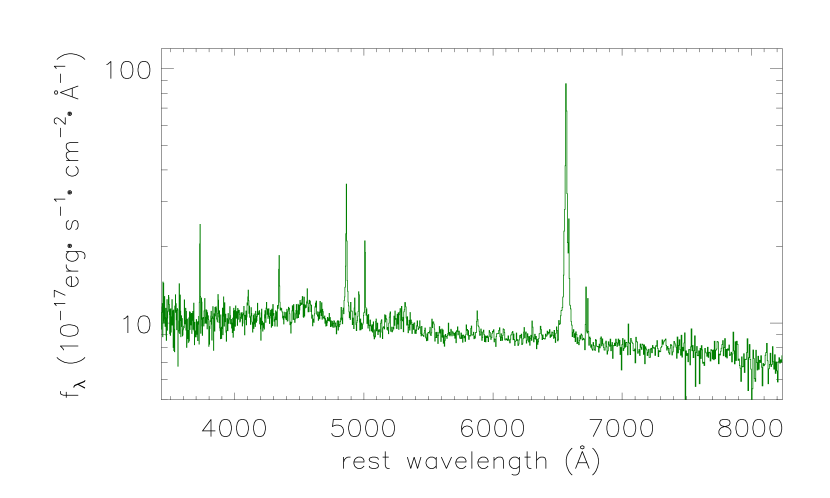
Figure 1: The SDSS fiber spectrum of SDSS J1042-0018.

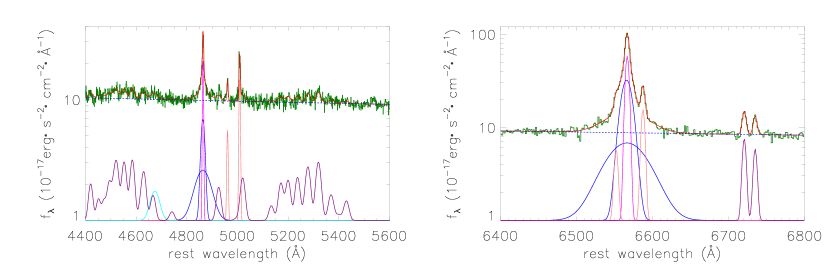
Figure 2: The best fitting descriptions to the emission lines around H$\beta$ (left panel) and H$\alpha$ (right panel) by multiple Gaussian functions plus power-law continuum emissions. In each panel, solid dark green line shows the SDSS spectrum, solid red line shows the determined best-fitting results, dashed blue line shows the determined power law continuum emissions. In left panel, solid blue lines show the determined broad H$\beta$ described by two broad Gaussian functions, solid purple line shows the determined optical Fe ii emission features, solid cyan line shows the determined broad He ii line, solid magenta line shows the determined narrow H$\beta$, solid pink line shows the determined core components in [O iii] doublet. In right panel, solid blue lines show the determined two broad components in broad H$\alpha$ described by two broad Gaussian functions, solid magenta line shows the determined narrow H$\alpha$, solid pink lines show the determined [N ii] doublet, and solid purple lines show the determined [S ii] doublet. In order to show clear emission features, the Y-axis is in logarithmic coordinate in each panel.

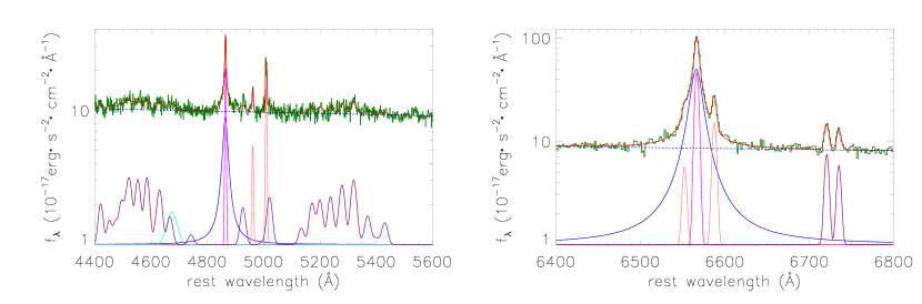
Figure 3: Same as Fig. 2, but the broad components in Balmer lines are described by Lorentz functions. In each panel, the solid blue line shows the Lorentz-function described broad Balmer line, the other line styles have the same meanings as those in Fig. 2.

2 Properties of spectroscopic emission lines of SDSS J1042-0018

Fig. 1 shows the SDSS spectrum of SDSS J1042-0018, with apparent broad emission lines indicating that SDSS J1042-0018  is undoubtfully a broad line AGN (type-1 AGN). In order to show the classification of SDSS J1042-0018  by flux ratios of narrow emission lines in the BPT diagram, the following emission line fitting procedures are applied to describe the emission lines of SDSS J1042-0018, especially the emission lines of narrow H$\beta$, narrow H$\alpha$, [O iii]$\lambda 4959,~{}5007$Å  doublet and [N ii]$\lambda 6548,~{}6583$Ådoublet which will be applied in the following BPT diagram, within rest wavelength from 4400 to 5600Å and from 6400 to 6800Å, which are fitted simultaneously by the following two different kinds of model functions. The fitting procedure is very similar as what we have done in Zhang & Feng (2016, 2017); Zhang (2021a, b, c), and simply described as follows.

For model A, Gaussian functions are applied to describe the emission lines as follows. Two narrow Gaussian functions are applied to describe the [O iii]$\lambda 4959,~{}5007$Å  doublet. Here, as the following shown best-fitting results, there is no necessary to consider extended components of both [O iii]$\lambda 4959,~{}5007$Å  doublet and the other narrow emission lines. Even two additional Gaussian components were applied to describe the probable extended components of [O iii]$\lambda 4959,~{}5007$Å  doublet and the other narrow emission lines, the determined line fluxes of the extended components near to zero and smaller than determined uncertainties. Therefore, the [O iii]$\lambda 4959,~{}5007$Å  doublet are clear in the SDSS J1042-0018. Two narrow Gaussian functions are applied to describe the narrow H$\beta$ and narrow H$\alpha$. Two broad Gaussian functions are applied to describe the broad H$\beta$. Two broad Gaussian functions are applied to describe the broad H$\alpha$. Two narrow Gaussian functions are applied to describe the [S ii]$\lambda 6716,6731$Å. One broad Gaussian function is applied to describe the broad He ii line. The broadened optical Fe ii template in Kovacevic et al. (2010) is applied to describe the optical Fe ii emission features. One power law component is applied to describe the AGN continuum emissions underneath the emission lines around H$\beta$. One power law component is applied to describe the AGN continuum emissions underneath the emission lines around H$\alpha$. For the model parameters of the model functions in model A, the following restrictions are accepted. First, the flux of each Gaussian component is not smaller than zero. Second, the flux ratio of the [O iii] doublet ([N ii] doublet) is fixed to the theoretical value 3. Third, the Gaussian components of each forbidden line doublet have the same redshift and the same line width in velocity space. There are no further restrictions on the parameters of Balmer emission lines.

For model B, the model functions are similar as the ones in model A, but the broad H$\beta$ (H$\alpha$) is described by one broad Lorentz function. And the same restrictions are accepted to the model parameters in model B. The main objective to consider Lorentz function to describe the broad Balmer lines is as follows. Not similar Gaussian function, Lorentz function always has sharp peak which can lead to more smaller measured fluxes of narrow Balmer lines, which will have positive effects on the classifications by flux ratios of narrow emission lines in BPT diagram, which will be discussed in the following section.

Through the Levenberg-Marquardt least-squares minimization technique, the emission lines around H$\beta$ and around H$\alpha$ can be well measured. The best fitting results are shown in Fig. 2 with $\chi^{2}/dof=1.18$ (summed squared residuals divided by degree of freedom) by model functions in model A, and in Fig 3 with $\chi^{2}/dof=1.19$ by model functions in model B. The line parameters of each Gaussian component of narrow emission lines, Gaussian and Lorentz describe broad Balmer lines, and the power law continuum emissions are listed in Table 1.

Table 1: Line parameters of the emission lines

name	$\lambda_{0}$	$\sigma$	flux	$\lambda_{0}$	$\sigma$	flux
	Gaussian Broad Balmer lines			Lorentz Broad Balmer lines
	$\chi^{2}/dof=1.18$			$\chi^{2}/dof=1.19$
H$\beta_{B1}$	4863.91$\pm$0.78	30.29$\pm$4.65	121$\pm$16	4863.54$\pm$0.42	20.28$\pm$2.22	247$\pm$11
H$\beta_{B2}$	4863.57$\pm$0.09	7.51$\pm$0.88	109$\pm$13	…	…	…
He ii	4674.16$\pm$4.88	17.63$\pm$4.83	34$\pm$8	4673.97$\pm$4.78	17.04$\pm$4.71	32$\pm$8
H$\beta_{N}$	4864.16$\pm$0.04	1.99$\pm$0.11	99$\pm$8	4864.23$\pm$0.05	1.98$\pm$0.11	98$\pm$8
[O iii]$\lambda 5007$Å(N)	5008.69$\pm$0.18	2.48$\pm$0.15	85$\pm$6	5008.73$\pm$0.18	2.44$\pm$0.15	83$\pm$6
H$\alpha_{B1}$	6566.27$\pm$1.06	26.49$\pm$1.24	384$\pm$20	6565.99$\pm$0.09	15.01$\pm$0.66	1150$\pm$20
H$\alpha_{B2}$	6565.81$\pm$0.12	7.38$\pm$0.24	575$\pm$19	…	…	…
H$\alpha_{N}$	6566.61$\pm$0.05	2.45$\pm$0.08	351$\pm$18	6566.70$\pm$0.06	2.27$\pm$0.11	262$\pm$24
[N ii]$\lambda 6583$Å	6587.33$\pm$0.12	2.35$\pm$0.12	86$\pm$5	6587.53$\pm$0.12	2.28$\pm$0.11	81$\pm$4
[S ii]$\lambda 6717$Å	6720.45$\pm$0.12	2.33$\pm$0.13	39$\pm$2	6720.45$\pm$0.12	2.36$\pm$0.12	39$\pm$2
[S ii]$\lambda 6731$Å	6734.83$\pm$0.12	2.34$\pm$0.13	28$\pm$2	6734.83$\pm$0.13	2.36$\pm$0.13	29$\pm$2
pow H$\beta$	$f_{\lambda}=(9.57\pm 0.04)(\frac{\lambda}{5100\textsc{\AA}})^{-0.52\pm 0.05}$			$f_{\lambda}=(9.57\pm 0.04)(\frac{\lambda}{5100\textsc{\AA}})^{-0.52\pm 0.05}$
pow H$\alpha$	$f_{\lambda}=(8.74\pm 0.04)(\frac{\lambda}{6563\textsc{\AA}})^{-1.74\pm 0.19}$			$f_{\lambda}=(8.56\pm 0.04)(\frac{\lambda}{6563\textsc{\AA}})^{-1.59\pm 0.19}$

Note: The first column shows the information of emission component listed. [O iii]$\lambda 5007$Å(N) mean the narrow component of [O iii]$\lambda 5007$Å. H$\beta_{N}$ and H$\alpha_{N}$ mean the narrow H$\beta$ and the narrow H$\alpha$. The ’pow H$\beta$’ and the ’pow H$\alpha$’ mean the power law continuum emissions around H$\beta$ and around H$\alpha$, respectively. The second column to the fourth column show the line parameters of central wavelength in unit of Å, second moment in unit of Å  and line flux in unit of $10^{-17}{\rm erg/\cdot~{}s^{-1}\cdot~{}cm^{-2}}$ of the determine components by Model A with two broad Gaussian functions (H$\beta_{B1}$, H$\beta_{B2}$ and H$\alpha_{B1}$, H$\alpha_{B2}$) applied to describe the broad Balmer lines. The fifth column to the seventh column show the line parameters of the determine components by Model B with one broad Lorentz function (H$\beta_{B1}$, H$\alpha_{B1}$) applied to describe the broad Balmer lines.

The different model functions clearly lead to quite different line parameters of narrow Balmer emission lines (especially line flux of narrow H$\alpha$) but similar line parameters of [O iii] and [N ii] doublets, which will lead to quite different flux ratios of [O iii] to narrow H$\beta$ (O3HB) and of [N ii] to narrow H$\alpha$ (N2HA).

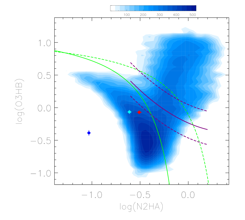
Figure 4: The BPT diagram for more than 35000 narrow line objects (contour in bluish colors) and the mis-classified broad line AGN SDSS J1042-0018  (solid circles in red, cyan, purple) by O3HB versus N2HA. Solid and dashed green lines show the dividing lines reported in Kauffmann et al. (2003) and in Kewley et al. (2001) between HII galaxies, composite galaxies and AGN. Solid purple line and dashed purple lines show the dividing line between HII galaxies and AGN and the area for composite galaxies determined in our recent work in Zhang et al. (2020) to determine the dividing lines in the BPT diagram through the powerful t-SNE technique. The contour is created by emission line properties of more than 35000 narrow emission-line galaxies discussed in Zhang et al. (2020) collected from SDSS DR15. Corresponding number densities to different colors are shown in the color bar. Solid circles in blue, cyan and red represent the results of [$N2HA_{LA}$, $O3HB_{LA}$], [$N2HA_{UA}$, $O3HB_{UA}$] and [$N2HA_{B}$, $O3HB_{B}$], respectively.

3 SDSS J1042-0018 in the BPT diagram

3.1 Flux ratios of narrow emission lines based on the model A

Based on the measured line parameters listed in Table 1 by model A, the H$\beta_{B1}$ and H$\alpha_{B1}$ are certainly from central BLRs, because of their line widths (second moment) quite larger than $900{\rm km\cdot~{}s^{-1}}$. The forbidden emission lines are certainly from central NLRs. Comparing with line widths of the [O iii] components, the determined narrow components of Balmer emissions, H$\beta_{N}$, and H$\alpha_{N}$, can be well accepted to come from central NLRs, because their line widths are smaller than the line width of the of [O iii] line.

Besides the emission components discussed above, the determined broad component H$\beta_{B2}$ and H$\alpha_{B2}$ have line width larger than the line width of [O iii] component but smaller than $900{\rm km\cdot~{}s^{-1}}$, it is hard to confirm the broad components of H$\beta_{B2}$ and H$\alpha_{B2}$ with line width about $400{\rm km\cdot~{}s^{-1}}$ are from central BLRs.

Finally, for the determined components shown in Fig. 2 and with parameters listed in the second column to the fourth column in Table 1, the [N ii] and [O iii] doublets and narrow Balmer lines are from central NLRs. Therefore, considering the H$\beta_{B2}$ and H$\alpha_{B2}$ coming from central NLRs, the lower limit of flux ratio of [O iii]$\lambda 5007$Å  to narrow H$\beta$ ( including two components of H$\beta_{N}$ and H$\beta_{B2}$) and lower limit of flux ratio of [N ii]$\lambda 6583$Å  to narrow H$\alpha$ (including two components of H$\alpha_{N}$ and H$\alpha_{B2}$) can be estimated as

$$\begin{split}O3HB_{LA}~{}=~{}\frac{f_{[O~{}\textsc{iii}]\lambda 5007\textsc{\AA}(N)}}{f_{H\beta_{N}}~{}+~{}f_{H\beta_{B2}}}~{}=~{}0.41\pm 0.04;\ \ \ \ \ \ \ \ N2HA_{LA}~{}=~{}\frac{f_{[N~{}\textsc{ii}]\lambda 6583\textsc{\AA})}}{f_{H\alpha_{N}}~{}+~{}f_{H\alpha_{B2}}}~{}=~{}0.093\pm 0.004\end{split}$$ (1)

If considering the H$\beta_{B2}$ and H$\alpha_{B2}$ coming from central BLRs, the upper limit of flux ratio of [O iii]$\lambda 5007$Å  to narrow H$\beta$ (only one component H$\beta_{N}$) and the upper limit of flux ratio of [N ii]$\lambda 6583$Å  to narrow H$\alpha$ (only one component H$\alpha_{N}$) can be estimated as

$$\begin{split}O3HB_{UA}~{}=~{}\frac{f_{[O~{}\textsc{iii}]\lambda 5007\textsc{\AA}(N)}}{f_{H\beta_{N}}}~{}=~{}0.86\pm 0.06;\ \ \ \ \ \ \ \ N2HA_{UA}~{}=~{}\frac{f_{[N~{}\textsc{ii}]\lambda 6583\textsc{\AA})}}{f_{H\alpha_{N}}}~{}=~{}0.245\pm 0.013\end{split}$$ (2)

Based on the determined narrow emission line ratios by model A, the SDSS J1042-0018  can be plotted in the BPT diagram of O3HB versus N2HA in Fig. 4. Considering the dividing lines in the BPT diagram as well discussed in Kauffmann et al. (2003); Kewley et al. (2006, 2019); Zhang et al. (2020), either [$N2HA_{UA}$, $O3HB_{UA}$] or [$N2HA_{LA}$, $O3HB_{LA}$] applied in the BPT diagram, the SDSS J1042-0018  can be well classified as a HII galaxy with few contributions of central AGN activities, through the properties of narrow emission lines.

3.2 Flux ratios of narrow emission lines based on the model B

For the results by model B, the determined H$\beta_{B1}$ and H$\alpha_{B1}$ have line widths quite larger than $900{\rm km\cdot s^{-1}}$, therefore, the determined H$\beta_{B1}$ and H$\alpha_{B1}$ can be safely accepted to be from central BLRs. Certainly, the forbidden narrow lines are considered and well accepted from the central NLRs. Then, comparing with the line width $150{\rm km\cdot~{}s^{-1}}$ of [O iii]$\lambda$5007Å, the determined components of narrow emission lines with line widths smaller than $150{\rm km\cdot~{}s^{-1}}$ can be safely accepted to be from central NLRs.

Finally, for the determined components shown in Fig. 3 and with parameters listed in the fifth column to the seventh column in Table 1, the broad components H$\beta_{B1}$, H$\alpha_{B1}$ are truly from central BLRs, the [N ii] and [O iii] doublets and narrow Balmer lines are from central NLRs. Therefore, flux ratio of [O iii]$\lambda 5007$Å  to narrow H$\beta$ can be estimated as

$$\begin{split}O3HB_{B}~{}=~{}\frac{f_{[O~{}\textsc{iii}]\lambda 5007\textsc{\AA}(N)}}{f_{H\beta_{N}}}~{}=~{}0.85\pm 0.06;\ \ \ \ \ \ \ \ N2HA_{B}~{}=~{}\frac{f_{[N~{}\textsc{ii}]\lambda 6583\textsc{\AA})}}{f_{H\alpha_{N}}}~{}=~{}0.31\pm 0.02\end{split}$$ (3)

Based on the model B, the SDSS J1042-0018  can be re-plotted in the BPT diagram of O3HB versus N2HA in Fig. 4. The SDSS J1042-0018  can be well classified as a HII galaxy with few contributions of central AGN activities, through the properties of narrow emission lines.

Finally, based on different model functions to describe emission lines and based on different considerations of emission components from central NLRs, the SDSS J1042-0018  can be well classified as a HII galaxy with few contributions of central AGN activities. In the manuscript, the SDSS J1042-0018  can be called as a mis-classified broad line AGN, based on the applications of BPT diagram.

4 Physical origin of the mis-classified broad line AGN SDSS J1042-0018?

In order to explain the mis-classified broad line AGN SDSS J1042-0018, two reasonable methods can be mainly considered in the section, as what we have discussed in SDSS J1451+2709 in Zhang (2021c). On the one hand, there is one mechanism leading to stronger narrow Balmer emissions, such as the strong starforming contributions. On the other hand, there is one mechanism leading to weaker forbidden emission lines, such as the expected high electron densities in central NLRs.

4.1 Strong Starforming contributions?

In the subsection, starforming contributions are checked, in order to explain the quite small value of O3HB, because of stronger starforming contributions leading to stronger narrow Balmer emission lines. In other words, there are two kinds of flux components included in the narrow Balmer lines and [O iii]$\lambda 5007$Å  and [N ii]$\lambda 6583$Å, one kind of flux depending on central AGN activities: $f_{[O~{}\textsc{iii}]}(AGN)$, $f_{[N~{}\textsc{ii}]}(AGN)$, $f_{H\alpha}(AGN)$ and $f_{H\beta}(AGN)$, the other kind of flux depending on starforming: $f_{[O~{}\textsc{iii}]}(SF)$, $f_{[N~{}\textsc{ii}]}(SF)$, $f_{H\alpha}(SF)$ and $f_{H\beta}(SF)$. Then, the measured flux ratio $O3HB$ and $N2HA$, and the flux rations $O3HB(AGN)$ and $N2HA(AGN)$ depending on central AGN activities, and the flux ratios $O3HB(SF)$ and $N2HA(SF)$ depending on starforming, can be described as

$$\begin{split}&O3HB~{}=~{}\frac{f_{[O~{}\textsc{iii}]}(AGN)~{}+~{}f_{[O~{}\textsc{iii}]}(SF)}{f_{H\beta}(AGN)~{}+~{}f_{H\beta}(SF)}\hskip 56.9055ptN2HA~{}=~{}\frac{f_{[N~{}\textsc{ii}]}(AGN)~{}+~{}f_{[N~{}\textsc{ii}]}(SF)}{f_{H\alpha}(AGN)~{}+~{}f_{H\alpha}(SF)}\\ &O3HB(AGN)~{}=~{}\frac{f_{[O~{}\textsc{iii}]}(AGN)}{f_{H\beta}(AGN)}\hskip 85.35826ptO3HB(SF)~{}=~{}\frac{f_{[O~{}\textsc{iii}]}(SF)}{f_{H\beta}(SF)}\\ &N2HA(AGN)~{}=~{}\frac{f_{[N~{}\textsc{ii}]}(AGN)}{f_{H\alpha}(AGN)}\hskip 85.35826ptN2HA(SF)~{}=~{}\frac{f_{[N~{}\textsc{ii}]}(SF)}{f_{H\alpha}(SF)}\\ &f_{[O~{}\textsc{iii}]}~{}=~{}f_{[O~{}\textsc{iii}]}(AGN)~{}+~{}f_{[O~{}\textsc{iii}]}(SF)\hskip 56.9055ptf_{[N~{}\textsc{ii}]}~{}=~{}f_{[N~{}\textsc{ii}]}(AGN)~{}+~{}f_{[N~{}\textsc{ii}]}(SF)\\ &f_{H\beta}~{}=~{}f_{H\beta}(AGN)~{}+~{}f_{H\beta}(SF)\hskip 85.35826ptf_{H\alpha}~{}=~{}f_{H\alpha}(AGN)~{}+~{}f_{H\alpha}(SF)\end{split}$$ (4)

where $f_{[O~{}\textsc{iii}]}$, $f_{[N~{}\textsc{ii}]}$, $f_{H\alpha}$ and $f_{H\beta}$ mean the measured total line fluxes of [O iii]$\lambda 5007$Å, [N ii]$\lambda 6583$Å  and narrow Balmer lines.

Based on the three measured data points shown in Fig. 4 and the corresponding measured total line fluxes $f_{[O~{}\textsc{iii}]}$, $f_{[N~{}\textsc{ii}]}$, $f_{H\alpha}$ and $f_{H\beta}$ listed in Table 1 and discussed in Section 3, expected properties of starforming contributions $R_{SF}~{}=~{}f_{H\alpha}(SF)/f_{H\alpha}$ can be simply determined, through the following limitations. First, the determined flux ratios of $O3HB(AGN)$ and $N2HA(AGN)$ clearly lead the data points classified as AGN in the BPT diagram, the data points lying above the dividing line shown as solid green line in Fig. 4. Second, the determined flux ratios of $O3HB(SF)$ and $N2HA(SF)$ clearly lead the data points classified as AGN in the BPT diagram, the data points lying below the dividing line shown as solid green line in Fig. 4. Third, the ratios of $f_{H\alpha}(SF)$ to $f_{H\alpha}(AGN)$ are similar as the ratios of $f_{H\beta}(SF)$ to $f_{H\beta}(AGN)$.

Based on the model A with considering H$\beta_{B2}$ and H$\alpha_{B2}$ from NLRs, the narrow emission line fluxes are about $f_{[O~{}\textsc{iii}]}~{}\sim~{}85$, $f_{[N~{}\textsc{ii}]}~{}\sim~{}86$, $f_{H\alpha}~{}\sim~{}926$ and $f_{H\beta}~{}\sim~{}208$ in the units of $10^{-17}{\rm erg\cdot~{}s^{-1}\cdot~{}cm^{-2}}$. Model simulating results can be simply done by the following three steps. First and foremost, based on the measured values of $f_{[O~{}\textsc{iii}]}$, $f_{[N~{}\textsc{ii}]}$, $f_{H\alpha}$ and $f_{H\beta}$, value of $f_{[O~{}\textsc{iii}]}(AGN)$ can be randomly selected from 0 to 85, leading to the fixed $f_{[O~{}\textsc{iii}]}(SF)~{}=~{}85~{}-~{}f_{[O~{}\textsc{iii}]}(AGN)$; value of $f_{[N~{}\textsc{ii}]}(AGN)$ can be randomly selected from 0 to 86, leading to the fixed $f_{[N~{}\textsc{ii}]}(SF)~{}=~{}86~{}-~{}f_{[N~{}\textsc{ii}]}(AGN)$; value of $f_{H\alpha}(AGN)$ can be randomly selected from 0 to 926, leading to the fixed $f_{H\alpha}(SF)~{}=~{}926~{}-~{}f_{H\alpha}(AGN)$ and leading to the values of $f_{H\beta}(AGN)$ and $f_{H\beta}(SF)$ determined by

$$\begin{split}&f_{H\beta}(AGN)~{}+~{}f_{H\beta}(SF)~{}=~{}208\\ &f_{H\beta}(AGN)~{}=~{}\frac{f_{H\alpha}(AGN)}{f_{H\alpha}(SF)}~{}\times~{}f_{H\beta}(SF)\end{split}$$ (5)

Besides, based on the randomly selected values of $f_{[O~{}\textsc{iii}]}(AGN)$, $f_{[N~{}\textsc{ii}]}(AGN)$, $f_{H\alpha}(AGN)$ and $f_{H\beta}(AGN)$, to determine whether the ratios of $O3HB_{s}~{}=~{}\frac{f_{[O~{}\textsc{iii}]}(AGN)}{f_{H\beta}(AGN)}$ and $N2HA_{s}~{}=~{}\frac{f_{[N~{}\textsc{ii}]}(AGN)}{f_{H\alpha}(AGN)}$ can lead to the data point [$O3HB_{s}$, $N2HA_{s}$] lying above the dividing line shown as solid green line in the BPT diagram of O3HB versus N2HA. Only if the data point [$O3HB_{s}$, $N2HA_{s}$] lies in the AGN region in the BPT diagram, the randomly selected values of $f_{[O~{}\textsc{iii}]}(AGN)$, $f_{[N~{}\textsc{ii}]}(AGN)$, $f_{H\alpha}(AGN)$ are appropriate values. Therefore, the randomly selected values each time are not always appropriate values. Last but not the least, after the first and the second steps are repeated tens of thousands of times, 5000 appropriate values can be collected for the $f_{[O~{}\textsc{iii}]}(AGN)$, $f_{[N~{}\textsc{ii}]}(AGN)$, and $f_{H\alpha}(AGN)$. Then, based on the results through the model A with considering H$\beta_{B2}$ and H$\alpha_{B2}$ from NLRs, among 66000 randomly selected values of $f_{[O~{}\textsc{iii}]}(AGN)$ from 0 to 85, of $f_{[N~{}\textsc{ii}]}(AGN)$ from 0 to 86 and of $f_{H\alpha}(AGN)$ from 0 to 926, there are 5000 couple data points of [$O3HB(AGN)$, $N2HA(AGN)$] classified as AGN, and corresponding 5000 couple data points of [$O3HB(SF)$, $N2HA(SF)$] classified as HII, in the BPT diagram of O3HB versus N2HA, shown in the left panel of Fig. 5. And top right panel of Fig. 5 shows the dependence of $R_{SF}(AL)$ on $N2HA(SF)(AL)$, with the determined minimum value 76% of the $R_{SF}(AL)$.

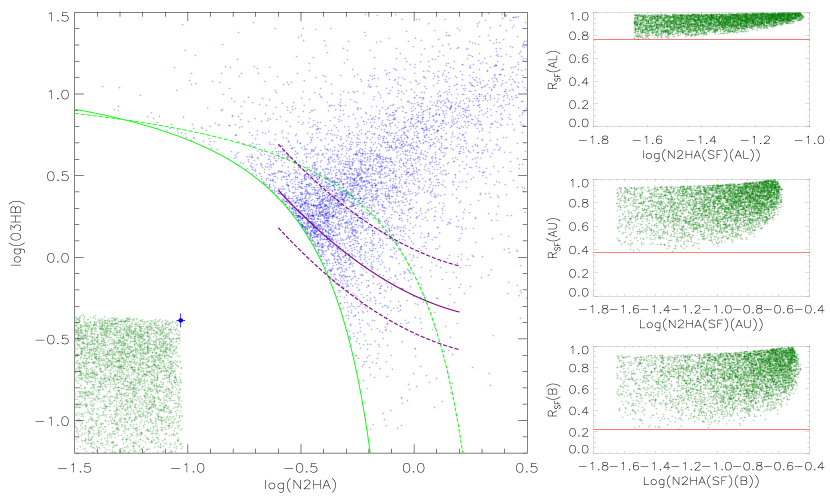
Figure 5: Left panel shows the simulated 5000 couple data points of [$O3HB(AGN)$, $N2HA(AGN)$] classified as AGN shown as blue pluses, and the simulated 5000 couple data points of [$O3HB(SF)$, $N2HA(SF)$] classified as HII shown as dark green pluses, in the BPT diagram of O3HB versus N2HA, based on the narrow line fluxes determined by model A with considering H$\beta_{B2}$ and H$\alpha_{B2}$ from central NLRs. The solid blue circle plus error bars and the line styles are the same as those shown in Fig. 4. Top right panel shows the dependence of $R_{SF}(AL)$ on $N2HA(SF)(AL)$, based on the narrow line fluxes determined by model A with considering H$\beta_{B2}$ and H$\alpha_{B2}$ from central NLRs. Middle right panel shows the dependence of $R_{SF}(AU)$ on $N2HA(SF)(AU)$, based on the narrow line fluxes determined by model A with considering H$\beta_{B2}$ and H$\alpha_{B2}$ from central BLRs. Bottom right panel shows the dependence of $R_{SF}(B)$ on $N2HA(SF)(B)$, based on the narrow line fluxes determined by model B. In each right panel, horizontal red line shows the position of the minimum value of $R_{SF}$.

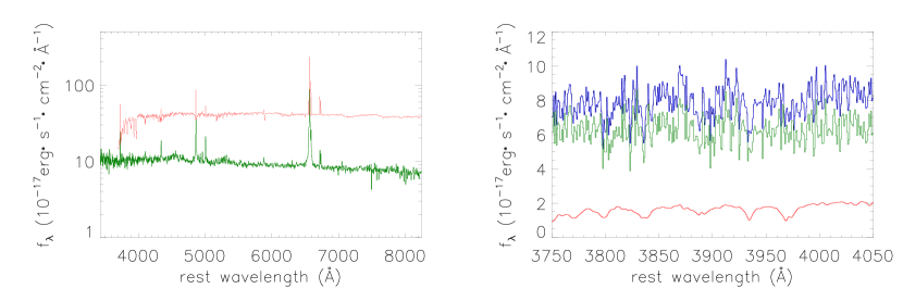
Figure 6: Left panel shows the SDSS spectrum of SDSS J1042-0018  in dark green and the mean spectrum of HII galaxies in red. Right panel shows the composite spectrum around 4000Å, including 20% starforming contributions. In right panel, solid blue line shows the composite spectrum, solid dark green line shows the SDSS spectrum, and solid red line shows the starforming contributions.

Similarly, based on the model A with considering H$\beta_{B2}$ and H$\alpha_{B2}$ from BLRs, the narrow emission line fluxes are about $f_{[O~{}\textsc{iii}]}~{}\sim~{}85$, $f_{[N~{}\textsc{ii}]}~{}\sim~{}86$, $f_{H\alpha}~{}\sim~{}351$ and $f_{H\beta}~{}\sim~{}99$ in the units of $10^{-17}{\rm erg\cdot~{}s^{-1}\cdot~{}cm^{-2}}$. Then, among 22000 randomly selected values of $f_{[O~{}\textsc{iii}]}(AGN)$, of $f_{[N~{}\textsc{ii}]}(AGN)$ and of $f_{H\alpha}(AGN)$, there are 5000 couple data points of [$O3HB(AGN)$, $N2HA(AGN)$] classified as AGN, and corresponding 5000 couple data points of [$O3HB(SF)$, $N2HA(SF)$] classified as HII, in the BPT diagram of O3HB versus N2HA. Here, we do not show the results in the BPT diagram, which are totally similar as the those shown in the left panel of Fig. 5. And the middle right panel of Fig. 5 shows the dependence of $R_{SF}(AU)$ on $N2HA(SF)(AU)$, with the determined minimum value 37% of the $R_{SF}(AU)$.

Based on the model B, the narrow emission line fluxes are about $f_{[O~{}\textsc{iii}]}~{}\sim~{}83$, $f_{[N~{}\textsc{ii}]}~{}\sim~{}81$, $f_{H\alpha}~{}\sim~{}262$ and $f_{H\beta}~{}\sim~{}98$ in the units of $10^{-17}{\rm erg\cdot~{}s^{-1}\cdot~{}cm^{-2}}$. Then, among 15000 randomly selected values of $f_{[O~{}\textsc{iii}]}(AGN)$, of $f_{[N~{}\textsc{ii}]}(AGN)$ and of $f_{H\alpha}(AGN)$, there are 5000 couple data points of [$O3HB(AGN)$, $N2HA(AGN)$] classified as AGN, and corresponding 5000 couple data points of [$O3HB(SF)$, $N2HA(SF)$] classified as HII, in the BPT diagram of O3HB versus N2HA. Here, we do not show the results in the BPT diagram, which are totally similar as the those shown in the left panel of Fig. 5. And the bottom right panel of Fig. 5 shows the dependence of $R_{SF}(B)$ on $N2HA(SF)(B)$, with the determined minimum value 22% of the $R_{SF}(B)$.

Therefore, the determined starforming contributions $R_{SF}$ should be larger than 22%. The strong starforming contributions indicate there should be apparent absorption features from host galaxy in the spectrum of SDSS J1042-0018. Fig. 6 shows one composite spectrum created by 0.8 times of the SDSS spectrum of SDSS J1042-0018  plus a mean HII galaxy with continuum intensity at 5100Å  about 0.2 times of the continuum intensity at 5100Å  of the SDSS spectrum of SDSS J1042-0018. Here, the mean spectrum of HII galaxies are created by the large sample of 1298 HII galaxies with signal-to-noise larger than 30 in SDSS DR12. There should be absorption features around 4000Å, clearly indicating that the starforming contributions could be well applied to explain the unique properties of the mis-classified broad line AGN SDSS J1042-0018.

Before the end of the subsection, there is one point we should note. As discussed in Kauffmann & Heckman (2009) for galaxies around the boundary as defined in Kauffmann et al. (2003), contributions to [O iii] emissions by star-formations are predicted to be typically 40 to 50%, which are roughly agreement with our determined $R_{SF}$ with minimum value of about 22% and with maximum value of about 76%, providing further clues to support the starforming contributions to explain the unique properties of the mis-classified broad line AGN SDSS J1042-0018. However, one probable question is proposed why we did not see apparent contribution of AGN activities to the narrow emission lines in SDSS J1042-0018? Actually, as the results shown in Fig. 5 for the simulating results, the separated appropriate contributions of AGN activities to narrow emission lines, $f_{[O~{}\textsc{iii}]}(AGN)$, $f_{[N~{}\textsc{ii}]}(AGN)$, $f_{H\alpha}(AGN)$, are randomly determined and lead to the data points on AGN activities apparently lying in the AGN region in the BPT diagram. Therefore, the SDSS J1042-0018  including AGN activities but lying in the HII region in the BPT diagram is mainly due to mixed contributions of star-formations and AGN activities, if considering starforming contributions as the preferred model to explain the unique properties of the mis-classified broad line AGN SDSS J1042-0018. Moreover, as the shown results in Fig. 5, there could be dozens of broad line quasars (a sample of tens of mis-classified quasars will be reported and discussed in one of our being prepared manuscripts) lying in the HII regions in the BPT diagrams with applications of narrow emission line properties. Certainly, intrinsic physical origin of the mis-classification in BPT diagram is still uncertain, further efforts are necessary.

4.2 Compressed central NLRs?

Besides the starforming contributions, high electron density in NLRs can be also applied to explain the unique properties of the mis-classified broad line AGN SDSS J1042-0018, because the high electron density near to the critical electron densities of the forbidden emission lines can lead to suppressed line intensities of forbidden emission lines but positive effects on strengthened Balmer emission lines.

It is not hard to determine electron density in NLRs, such as through the flux ratios of [S ii]$\lambda 6717,6731$Å  doublet as well discussed in Proxauf et al. (2014); Sanders et al. (2016); Kewley et al. (2019). Based on the measured line fluxes of [S ii] doublet listed in Table 1, the flux ratio of [S ii]$\lambda 6716$Å  to [S ii]$\lambda 6731$Å  lead the electron density to be estimated around ${\rm 200cm^{-3}}$, a quite normal value, quite smaller than the critical densities around ${\rm 10^{5}cm^{-3}}$ to [O iii] and [N ii] doublet.

5 Summaries and Conclusions

Finally, we give our summaries and conclusions as follows.

• Emission lines of the blue quasar SDSS J1042-0018  can be well measured by two different models, broad Balmer lines described by mode A with broad Gaussian functions and by model B with broad Lorentz functions, leading to different flux ratios of narrow emission lines.

• Different flux ratios of narrow emission lines determined by different model functions and with different considerations, the SDSS J1042-0018  can be well classified as a HII galaxy in the BPT diagram (a mis-classified broad line AGN), although the SDSS J1042-0018  actually is a normal broad line AGN.

• Two reasonable methods are proposed to explain the unique properties of the mis-classified broad line AGN SDSS J1042-0018, strong starforming contributions leading to stronger narrow Balmer emissions, and compressed NLRs with high electron densities leading to suppressed forbidden emissions.

• Once considering the starforming contributions, at least 20% starforming contributions should be preferred in the mis-classified broad line AGN SDSS J1042-0018, which will lead to apparent absorption features around 4000Å, indicating strong starforming contributions should be preferred in the mis-classified broad line AGN SDSS J1042-0018.

• Once considering the compressed NLRs with high electron densities, the expected electron densities should be around ${\rm 10^{5}cm^{-3}}$. However, the estimated electron density is only around ${\rm 200cm^{-3}}$ based on the flux ratio of [S ii]$\lambda 6716$Å  to [S ii]$\lambda 6731$Å. Therefore, the compressed NLRs with high electron densities are not preferred in the mis-classified broad line AGN SDSS J1042-0018.

• The reported second mis-classified broad line AGN SDSS J1042-0018  strongly indicate that there should be extremely unique properties of SDSS J1042-0018  which are currently not detected, or indicate that there should be a small sample of mis-classified broad line AGN similar as the SDSS J1042-0018.

• Narrow emission line properties should be carefully determined in Type-1 AGN.