Local breaking of the spin degeneracy in the vortex states of Ising superconductors: Induced antiphase ferromagnetic order

Abstract

Ising spin-orbital coupling is usually easy to identify in the Ising superconductors via an in-plane critical field enhancement, but we show that the Ising spin-orbital coupling also manifests in the vortex physics for perpendicular magnetic fields. By self-consistently solving the Bogoliubov-de Gennes equations of a model Hamiltonian built on the honeycomb lattice with the Ising spin-orbital coupling pertinent to the transition metal dichalcogenides, we numerically investigate the local breaking of the spin and sublattice degeneracies in the presence of a perpendicular magnetic field. It is revealed that the ferromagnetic orders are induced inside the vortex core region by the Ising spin-orbital coupling. The induced magnetic orders are antiphase in terms of their opposite polarizations inside the two nearest-neighbor vortices with one of the two polarizations coming dominantly from one sublattice sites, implying the local breaking of the spin and sublattice degeneracies. The finite-energy peaks of the local-density-of-states for spin-up and spin-down in-gap states are split and shifted oppositely by the Ising spin-orbital coupling, and the relative shifts of them on sublattices $A$ and $B$ are also of opposite algebraic sign. The calculated results and the proposed scenario may not only serve as experimental signatures for identifying the Ising spin-orbital coupling in the Ising superconductors, but also be prospective in manipulation of electron spins in motion through the orbital effect in the superconducting vortex states.

I introduction

The superconductivity uncovered in atomically thin two-dimensional (2D) forms of layered transition metal dichalcogenides (TMDs) have recently attracted remarkable scientific and technical interests Bromley1 ; Boker1 ; Zhu1 ; Xiao1 ; JTYe1 ; Taniguchi1 ; Kormanyos1 ; Zahid1 ; Cappelluti1 ; XXi1 ; WShi1 ; jmlu1 ; Saito1 ; XXi2 . Although these superconductors belong to the conventional $s$-wave superconductivity with low transition temperature Bromley1 ; Boker1 ; Zhu1 ; Xiao1 ; JTYe1 ; Taniguchi1 ; Kormanyos1 ; Zahid1 ; Cappelluti1 ; XXi1 ; WShi1 ; jmlu1 ; Saito1 ; XXi2 , the uniqueness of the TMDs makes them alluring to the researchers. On one hand, similar to graphene, these materials have a honeycomb lattice structure, and exhibit a valley degree of freedom with minima/maxima of conduction/valence bands at the corners $\mathbf{K}$ and $-\mathbf{K}$ of the Brillouin zone. On the other hand, unlike graphene, the in-plane mirror symmetry is broken in the TMDs, leading to a strong atomic Ising type spin-orbital coupling (ISOC) Zhu1 ; Xiao1 ; Kormanyos1 ; Zahid1 ; Cappelluti1 . The ISOC strongly pins the electron spins to the out-of-plane directions and have opposite directions in opposite valleys ($\mathbf{K}$ and $-\mathbf{K}$) Zhu1 ; Xiao1 ; Kormanyos1 ; Zahid1 ; Cappelluti1 ; jmlu1 ; XXi2 ; btzhou1 ; Sharma1 , so that it preserves time-reversal symmetry and is compatible with superconductivity. Due to the strong pinning of electron spins in the out-of-plane directions, external in-plane magnetic fields are much less effective in aligning electron spins, and lead to the in-plane upper critical field $H_{c2}$ of the system several times larger than the Pauli limit XXi1 ; jmlu1 .

Nevertheless, an out-of-plane magnetic field will generate the magnetic flux in conductors due to the dominating orbital effect over the Zeeman splitting. It is well known that the superconductors expel the magnetic flux from their interior, the so called Meissner effect. While some superconductors expel the magnetic field globally (they are called type I superconductors), a type II superconductor will only keep the whole magnetic field out until a first critical field $H_{c1}$ is reached. Then vortices start to appear. A vortex is a local magnetic flux quantum that penetrates the superconductor, where the superconducting (SC) order parameter drops to zero to save the rest of the SC state in metal from being destroyed. While the ISOC exemplifies itself as the spin-valley locking in the momentum space, it acts as coupling between spins and the orbital derived effectively periodic spin and sublattice dependent fluxes in real space with the quantization axis along the out-of-plane direction. This is to say the spins, sublattices and the effectively periodic fluxes are bound together by the ISOC in real space. Thus, the local breaking of the spin and sublattice degeneracies may be expected if the fluxes are altered locally, and the spin orders in real space may also be expected to emerge.

In this paper, we numerically demonstrate that the spin and sublattice degeneracies break locally with an induced ferromagnetic order inside the vortex core of the Ising superconductors, as a result of the contrasting variation of the effectively periodic fluxes for sublattices $A$ and $B$ caused by the out-of-plane magnetic field. By self-consistently solving the Bogoliubov-de Gennes (BdG) equations of the Hamiltonian, it is shown that there is no magnetic order induced inside the vortex core when the ISOC is zero. Accordingly, the curves of the local-density-of-states (LDOS) for the spin-up and spin-down in-gap states are almost identical, forming a series of discrete energy peaks inside the core region. The inclusion of the ISOC induces a ferromagnetic order inside the vortex core, where the SC order parameter is suppressed. The induced magnetic orders are antiphase in terms of their opposite polarizations inside two nearest-neighbor (NN) vortices with one of the two polarizations coming dominantly from one sublattice sites. The finite-energy peaks of the LDOS for spin-up and spin-down in-gap states are shifted oppositely by the ISOC, and the sign of the relative shifts of them depends on which sublattices the site is belonging to. Based on a scenario of local breaking of the spin and sublattice degeneracies due to the interaction of the ISOC derived effective fluxes with the local magnetic flux inside the vortex core, we give an explanation to the unusual phenomena regarding the polarization of the induced magnetic orders and the energy shifts of the finite-energy in-gap peaks. The calculated results may not only serve as experimental signatures for identifying the ISOC proposed in the Ising superconductors, but also put forward effective thinking-ways in manipulation of electron spins in motion through the orbital effect in the SC vortex states.

The remainder of the paper is organized as follows. In Sec. II, we introduce the model Hamiltonian and carry out analytical calculations. In Sec. III, we present numerical calculations and discuss the results. In Sec. IV, we make a conclusion.

II THEORY AND METHOD

The effective electron hoppings between the NN sites $i$ and $i+\tau_{j}$ on a honeycomb lattice can be described by the following tight-binding Hamiltonian,

$$H_{0} = -\sum_{i,\tau_{j},\sigma}(t_{i,i+\tau_{j}}a^{{\dagger}}_{i,\sigma}b_{i+\tau_{j},\sigma}+h.c.)-\mu(\sum_{i\in A,\sigma}a^{{\dagger}}_{i,\sigma}a_{i,\sigma}$$ (1)

$$+\sum_{i\in B,\sigma}b^{{\dagger}}_{i,\sigma}b_{i,\sigma}),$$

where $t_{i,i+\tau_{j}}$ is the hopping integral between the NN sites. $\mathbf{\tau}_{j}$ denotes the three NN vectors with $\mathbf{\tau}_{0}=a(\frac{\sqrt{3}}{2},\frac{1}{2})$, $\mathbf{\tau}_{1}=a(-\frac{\sqrt{3}}{2},\frac{1}{2})$ and $\mathbf{\tau}_{2}=a(0,-1)$ as defined in Fig. 1(a) with $a$ being the lattice constant. $a^{{\dagger}}_{i,\sigma}(b^{{\dagger}}_{i,\sigma})$ is the electron creation operator in sublattice $A$ $(B)$ if $i\in$ sublattice $A$ $(B)$, and $\mu$ the chemical potential. For the free hopping case with $t_{i,i+\tau_{j}}=t$, the Hamiltonian $H_{0}$ can be written in the momentum space,

$$H_{0}(k) = \sum_{k,\sigma}[\xi_{k}a^{{\dagger}}_{k,\sigma}b_{k,\sigma}+\xi^{\ast}_{k}b^{{\dagger}}_{k,\sigma}a_{k,\sigma}-\mu(a^{{\dagger}}_{k,\sigma}a_{k,\sigma}$$ (2)

$$+b^{{\dagger}}_{k,\sigma}b_{k,\sigma})],$$

where

$$\xi_{k}=-t\sum_{j=0}^{2}e^{i\mathbf{k}\cdot\mathbf{\tau}_{j}}.$$ (3)

One can readily find the energy bands for this Hamiltonian as neto1 ,

$$\varepsilon^{\pm}_{k} = \pm t[3+2\cos(\sqrt{3}k_{x})+4\cos(\sqrt{3}k_{x}/2)\cos(3k_{y}/2)]^{\frac{1}{2}}$$ (4)

$$-\mu.$$

with $+$ ($-$) indexing the conduction (valence) band. We focus on systems which have been doped such that the chemical potential $\mu$ lies in the upper conduction bands, and produce six spin degenerate pockets at the corners of the hexagonal Brillouin zone when $\varepsilon^{+}_{k}=0$, as shown in Fig. 1(b).

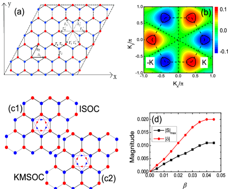
Figure 1: (a) Honeycomb lattice structure of the Ising superconductor, made out of two sublattices $A$ (blue dots) and $B$ (red dots). $\tau_{0}$, $\tau_{1}$ and $\tau_{2}$ are the nearest-neighbor vectors, and $\tau^{\prime}_{1}$-$\tau^{\prime}_{6}$ the next-nearest-neighbor vectors. (b) The Brillouin zone (dashed line) and the six spin degenerate Fermi pockets (solid lines) of the Ising superconductor. The red and blue colors indicate the opposite sign of the effective Zeeman fields between adjacent Fermi pockets located at $\mathbf{K}$ and $-\mathbf{K}$. The positive phase hopping directions for spin-up electrons depicted by $H_{ISOC}$ in Eq. (6) (c1), and by $H_{KM}$ in Eq. (15) (c2), respectively. The arrows in both figures indicate the positive phase hopping directions. (d) The ISOC dependencies of the maximum of the absolute value for the induced magnetic order $|S|_{max}$ and the magnitude of the relative energy shifts $|\delta|$ between the spin-up and spin-down in-gap state peaks on the vortex core center [reference to text and Fig. 4(b)].

The ISOC acts as strong effective Zeeman fields, which polarize electron spins oppositely to the out-of-plane direction at opposite valleys, that is, at the $\mathbf{K}$ and $-\mathbf{K}$ points in Fig. 1(b). If we choose the out-of-plane direction as the $z$-axis, the ISOC term has the form Frigeri1

$$H_{ISOC}(k)=\beta\sum_{k,\sigma,\sigma^{\prime}}\mathbf{g}_{k}\cdot\mathbf{\hat{\sigma}}_{\sigma\sigma^{\prime}}(a^{{\dagger}}_{k,\sigma}a_{k,\sigma^{\prime}}+b^{{\dagger}}_{k,\sigma}b_{k,\sigma^{\prime}}),$$ (5)

where $\beta$ is the ISOC strength, and $\hat{\sigma}$ denotes the Pauli matrices acting in the spin space. The ISOC requires that the form factor $\mathbf{g}_{k}$ alternates its sign between adjacent Fermi pockets located at $\mathbf{K}$ and $-\mathbf{K}$ [see Fig. 1(b)], which should be the form $\mathbf{g}_{k}=\hat{z}F_{k}$ with $F_{k}=2\sin(\sqrt{3}k_{x})-4\cos(3k_{y}/2)\sin(\sqrt{3}k_{x}/2)=-F_{-k}$ satisfying the time-reversal symmetry. In this way, the spins are bound to the orbitals in the momentum space and accordingly exhibit various valley dependent behaviors such as valley spintronics in these materials Radisavljevic ; Zhang1 ; Wang1 ; Bao1 ; Lee1 . By making the Fourier transformation of $F_{k}$, the ISOC term in real space can be reached as Jiang1 ,

$$H_{ISOC}=i\beta\sum_{i,\mathbf{\tau}^{\prime}_{j},\sigma,\sigma^{\prime}}\hat{\sigma}^{z}_{\sigma\sigma^{\prime}}(-1)^{j}(a^{{\dagger}}_{i,\sigma}a_{i+\mathbf{\tau}^{\prime}_{j},\sigma^{\prime}}+b^{{\dagger}}_{i,\sigma}b_{i+\mathbf{\tau}^{\prime}_{j},\sigma^{\prime}}),$$ (6)

where the vectors $\mathbf{\tau}^{\prime}_{j}$ connecting the six next-nearest-neighbor (NNN) sites are located at $\mathbf{\tau}^{\prime}_{1}=-\mathbf{\tau}^{\prime}_{4}=\sqrt{3}a(1,0)$, $\mathbf{\tau}^{\prime}_{2}=-\mathbf{\tau}^{\prime}_{5}=\sqrt{3}a(\frac{1}{2},\frac{\sqrt{3}}{2})$ and $\mathbf{\tau}^{\prime}_{3}=-\mathbf{\tau}^{\prime}_{6}=\sqrt{3}a(-\frac{1}{2},\frac{\sqrt{3}}{2})$, as indicated by the dashed arrows in Fig. 1(a). We will see later that the ISOC in real space depicted by Eq. (6) plays the role of the coupling between spins and the effectively periodic fluxes with the quantization axis along the out-of-plane direction. Then, the Hamiltonian including both the free hoppings and the ISOC term is reached, in real space as,

$$H_{TMD}=H_{0}+H_{ISOC}.$$ (7)

The SC pairing is assumed to be derived from the effective attraction between electrons,

$$H_{P} = \frac{V_{0}}{2}\sum_{i,\sigma}n_{i,\sigma}n_{i,\bar{\sigma}}.$$ (8)

Here, we consider the on-site interactions with $V_{0}$ denoting the effective interaction potential btzhou1 ; Sharma1 . By making the mean-field decoupling, $H_{P}$ can be rewritten in terms of the SC pairings as,

$$H_{P} = \sum_{i\in A}(\Delta_{A}a^{{\dagger}}_{i,\uparrow}a^{{\dagger}}_{i,\downarrow}+h.c.)+\sum_{i\in B}(\Delta_{B}b^{{\dagger}}_{i,\uparrow}b^{{\dagger}}_{i,\downarrow}$$ (9)

$$+h.c.),$$

where $\Delta_{A}=-V_{0}\langle a_{i,\uparrow}a_{i,\downarrow}\rangle$ ($\Delta_{B}=-V_{0}\langle b_{i,\uparrow}b_{i,\downarrow}\rangle$) defines the on-site spin-singlet $s$-wave SC pairing.

Then the total Hamiltonian is arrived as follows,

$$H=H_{TMD}+H_{pair}.$$ (10)

Based on the Bogoliubov transformation, the diagonalization of the Hamiltonian $H$ can be achieved by solving the following discrete BdG equations,

$$\sum_{j}\left(\begin{array}[]{cccc}-\mu\delta_{ij}&H_{ij,\uparrow\uparrow}&\Delta_{A}\delta_{ij}&0\\ H^{\ast}_{ij,\uparrow\uparrow}&-\mu\delta_{ij}&0&\Delta_{B}\delta_{ij}\\ \Delta^{\ast}_{A}\delta_{ij}&0&\mu\delta_{ij}&-H^{\ast}_{ij,\downarrow\downarrow}\\ 0&\Delta^{\ast}_{B}\delta_{ij}&-H_{ij,\downarrow\downarrow}&\mu\delta_{ij}\end{array}\right)\left(\begin{array}[]{cccc}u_{A,n,j,\uparrow}\\ u_{B,n,j,\uparrow}\\ v_{A,n,j,\downarrow}\\ v_{B,n,j,\downarrow}\end{array}\right)=$$ (19)

$$E_{n}\left(\begin{array}[]{cccc}u_{A,n,i,\uparrow}\\ u_{B,n,i,\uparrow}\\ v_{A,n,i,\downarrow}\\ v_{B,n,i,\downarrow}\end{array}\right),$$ (24)

where,

$$H_{ij,\uparrow\uparrow}=-t_{ij}\delta_{i+\mathbf{\tau}_{j},j}+i\beta\sigma^{z}_{\uparrow\uparrow}(-1)^{j}\delta_{i+\mathbf{\tau}^{\prime}_{j},j},$$

$$H_{ij,\downarrow\downarrow}=-t_{ij}\delta_{i+\mathbf{\tau}_{j},j}+i\beta\sigma^{z}_{\downarrow\downarrow}(-1)^{j}\delta_{i+\mathbf{\tau}^{\prime}_{j},j},$$ (25)

with $u_{A,n,j,\uparrow}$ ($u_{B,n,j,\uparrow}$) and $v_{A,n,j,\downarrow}$ ($v_{B,n,j,\downarrow}$) being the Bogoliubov quasiparticle amplitudes on the $j$-th site with corresponding eigenvalues $E_{n}$. The SC pairing amplitudes satisfy the following self-consistent conditions,

$$\Delta_{A}=-\frac{V_{0}}{2}\sum_{n}u_{A,n,i,\uparrow}v^{\ast}_{A,n,i,\downarrow}\tanh(\frac{E_{n}}{2k_{B}T}),$$

$$\Delta_{B}=-\frac{V_{0}}{2}\sum_{n}u_{B,n,i,\uparrow}v^{\ast}_{B,n,i,\downarrow}\tanh(\frac{E_{n}}{2k_{B}T}).$$ (26)

The spin dependent electron density $n_{A(B),i,\sigma}$ and the local magnetic orders $S_{A(B),i,z}$ are determined respectively by,

$$n_{A(B),i,\uparrow}=\sum_{n}|u_{A(B),n,i,\uparrow}|^{2}f(E_{n}),$$

$$n_{A(B),i,\downarrow}=\sum_{n}|v_{A(B),n,i,\downarrow}|^{2}f(E_{n}),$$

$$S_{A(B),i,z}=\frac{1}{2}[n_{A(B),i,\uparrow}-n_{A(B),i,\downarrow}].$$ (27)

III results and discussion

In numerical calculations, we choose the zero field hopping integral $t=200$meV as the energy unit, and fix temperature $T=1\times 10^{-5}$, unless otherwise specified. The filling factor $n=\sum_{i,\sigma}n_{i,\sigma}/N=1.08$ ($N$ denotes the number of total lattice sites) such that the chemical potential $\mu$ lies in the upper conduction band and gives rise to the Fermi surfaces in Fig. 1(b). In the presence of a perpendicular magnetic field, the orbital effect dominates over the the Zeeman splitting, so we neglect the Zeeman term of the external magnetic field in the following calculations. In this case, the hopping terms are described by the Peierls substitution. For the NN hopping between sites $i$ and $i+\mathbf{\tau}_{j}$, one has $t_{i,i+\mathbf{\tau}_{j}}=te^{i\varphi_{i,i+\mathbf{\tau}_{j}}}$, and for the NNN hopping between $i$ and $i+\mathbf{\tau}^{\prime}_{j}$ one should have $\beta\rightarrow\beta e^{i\varphi_{i,i+\mathbf{\tau}^{\prime}_{j}}}$, where $\varphi_{i,i+\mathbf{\tau}_{j}(\mathbf{\tau}^{\prime}_{j})}=\frac{\pi}{\Phi_{0}}\int^{r_{i}}_{r_{i+\mathbf{\tau}_{j}(\mathbf{\tau}^{\prime}_{j})}}\mathbf{A}(\mathbf{r})\cdot d\mathbf{r}$ with $\Phi_{0}=\frac{hc}{2e}$ being the SC flux quanta. We consider a system with a parallelogram vortex unit cell as shown in Fig. 1(a), where two vortices are accommodated. The vortex unit cell with size of $24\mathbf{a_{1}}\times 48\mathbf{a_{2}}$ is adopted in the calculations, unless otherwise stated. The vector potential $\mathbf{A}(\mathbf{r})=(0,Bx,0)$ is chosen in the Landau gauge to give rise to the magnetic field $\mathbf{B}$ along the $z$-direction.

In this study, we have no ambition to explore the SC mechanism underlying the Ising superconductors. Instead, we assume a phenomenological pairing potential $V_{0}$ to give rise to the SC pairing. Within the BCS theory, the coherence length is given by $\xi_{0}=\hbar v_{F}/\pi\Delta$, where $v_{F}$ is the Fermi velocity, linking the coherence length to the inverse size of the SC gap $\Delta$. The coherence length of NbSe₂ is about $10$nm as obtained from $H_{c2}(T)$ measurement Fente1 ; Kogan1 . The estimated vortex core size is of $\xi_{V}\sim 30$nm Fente1 . A system contains two such vortex cores would be larger than the size of $60$nm$\times 120$nm, which roughly amounts to a parallelogram sample with the size larger than $200\mathbf{a}_{1}\times 400\mathbf{a}_{2}$. Such a large size is far beyond the computational capability. However, it is still capable of mimicking the vortex physics on a relative small size of sample by artificially enlarging the SC gap $\Delta$. In the self-consistent calculations, the length scale of the sample with size $24\mathbf{a}_{1}\times 48\mathbf{a}_{2}$ is about one order smaller than the actual size. Thus, we need to choose a large $V_{0}=1.6$ in the self-consistent calculations to give rise to a bulk value of $\Delta\approx 0.09\sim 18$meV, a value about one order larger than the actual measurements Fente1 , so as to meet the requirement.

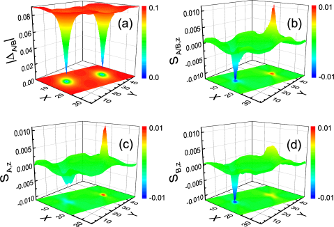
Figure 2: The spatial distributions of the SC and magnetic order parameters in the vortex states for $\beta=0.04$ are shown in (a) and (b), respectively. The spatial distributions of the magnetic order in the vortex states for $\beta=0.04$ on sublattice $A$ (c), and on sublattice $B$ (d), respectively.

III.1 The induced antiphase magnetic orders inside vortex cores

Under a perpendicular magnetic field, the vanishment of the screening current density at the vortex center drives the system into the vortex states with the suppression of the SC order parameter around the vortex core. In the absence of the ISOC interaction, we find that except for the suppression of the SC order around the vortex core region there is no other order to be induced. On the other hand, when the ISOC is present, a ferromagnetic order can emerge inside the vortex core region with its maximum appearing at the vortex core center. The maximum of the absolute value for the magnetic order $|S|_{max}$ exhibits roughly linear increasing trend with $\beta$ in a wide range of ISOC, and finally reaches a saturated value at large ISOC, as displayed in Fig. 1(d). Typical results on the vortex structure with $\beta=0.04$ are shown in Figs. 2(a) and 2(b) for the spatial distributions of SC and magnetic orders, respectively. As shown in Fig. 2(a), each vortex unit cell accommodates two SC vortices each carrying a flux quantum $\Phi_{0}$. The SC order parameter $|\Delta_{A/B}|$ vanishes at the vortex core center where the maximum of the induced magnetic order appears. It is interesting to note that the magnetic order parameters have opposite polar directions around two NN vortices along the long side of the parallelogram vortex unit cell, as shown in Fig. 2(b). The most unusual aspect of the spatial distribution of the magnetic order parameters $S_{A(B),i,z}$ appears when we replot in Figs. 2(c) and 2(d) the magnetic orders separately on the sublattices $A$ and $B$. Specifically, the positive magnetic order alone $z$-axis inside one vortex comes dominantly from the $A$ sublattice while the negative one inside another vortex comes dominantly from the $B$ sublattice.

In order to understand the origin as well as the unusual distributions of the induced magnetic order, we should note the fact that there is no magnetic order induced when ISOC is zero. In real space, the ISOC depicted by Eq. (6) plays the role of coupling between spins and the effectively periodic fluxes with the quantization axis along the out-of-plane direction. Following the ISOC term in Eq. (6), we display the positive phase [noting that $i=e^{i\pi/2}$] hopping directions of ISOC in Fig. 1(c1) by arrows on NNN bonds for spin-up electrons at sublattices $A$ and $B$, from which the effective spin fluxes are generated. If the positive phase hoppings on NNN bonds for spin-up electrons on sublattice $A$ generate spin flux pointing to $z$-direction, then they generate spin flux pointing to $-z$-direction on sublattice $B$, and contrary is true for spin-down electrons. That is, the NNN hoppings have opposite chirality, for sublattices $A$ and $B$. Since the spins, sublattices and the effectively periodic fluxes are bound together in real space, local breaking of the spin and sublattice degeneracies may be expected if the effective fluxes for sublattices $A$ and $B$ are contrastively altered by an out-of-plane magnetic field, and thus the spin orders in real space may also be expected. Nevertheless, we can not expect the appearance of magnetic order in the normal state under an out-of-plane magnetic field. This is due to the fact that the energy scale of the hopping integral $t$ overwhelms the ISOC strength $\beta$, interchanging the electrons between sites of sublattices $A$ and $B$ leading to the suppression of the local orders. However, the situation is totally different in the vortex state, where the localized electrons in the vortex core, which come from the breaking of the Cooper pairs, contribute to the magnetic order. If one vortex core resides on the $A$ sublattice site, the blue site shown in Fig. 1(a), the positive phase hoppings on NNN bonds bound to spin-up electrons on sublattice $A$ generate effective spin flux pointing to $z$-direction [noting the negative charge of the electrons], which is in the same direction as the magnetic field. On the contrary, the spin-down electrons on sublattice $A$ generate effective spin flux in the opposite direction of the magnetic field. Thus, the spin degeneracy breaks locally to two branches with a lower energy for the spin-up electrons, leading to the positive magnetic order around one vortex as shown in Fig. 2(c) on sublattice $A$. In principle, the pairing breaking from the spin-singlet SC pairings due to the orbital effect of the magnetic field results in equal numbers of spin-up and spin-down electrons, so the total spins should be zero as a global. The excess of spin-down electrons accumulate into the NN vortex to give rise to the negative magnetic order shown in Fig. 2(d) on sublattice $B$, whereby it saves the energy as the effective spin flux generated by spin-down electrons being in compliance with the direction of the magnetic field.

Two situations could lend support to the above scenario. Firstly, we consider the case with a reversal of the direction of the magnetic field, i.e., a magnetic field in the $-z$-direction. From the above argument, the polarizations of the induced magnetic orders should be reversed if the magnetic field reverses its direction. It is exactly the case as evidenced in Figs. 3(a) and 3(b), where the results are obtained with an out-of-plane magnetic field in the $-z$-direction while keep other parameters the same as that in Fig. 2. Secondly, we should make a comparison with the spin-orbital coupling (SOC) term in Kane-Mele model Kane1 , which has the form

$$H_{KM}=i\beta\sum_{i,\mathbf{\tau}^{\prime}_{j},\sigma,\sigma^{\prime}}\hat{\sigma}^{z}_{\sigma\sigma^{\prime}}(-1)^{j}(a^{{\dagger}}_{i,\sigma}a_{i+\mathbf{\tau}^{\prime}_{j},\sigma^{\prime}}-b^{{\dagger}}_{i,\sigma}b_{i+\mathbf{\tau}^{\prime}_{j},\sigma^{\prime}}).$$ (28)

Both $H_{ISOC}$ and $H_{KM}$ preserve time-reversal symmetry, so the spins remain degenerate in both cases. The only difference lies that $H_{ISOC}$ preserves the sublattice symmetry but $H_{KM}$ breaks it. As a result, the NNN hopping phases carried by the same spins in $H_{KM}$ would have same chirality for sublattices $A$ and $B$, as denoted by arrows in Fig. 2(c2). According to the above scenario, we deduce that the induced magnetic orders should be in the same direction for the two adjacent vortices. This is also verified in Figs. 3(c) and 3(d), where the results for the spatial distribution of the induced magnetic orders are calculated by replacing $H_{ISOC}$ with $H_{KM}$ while other parameters remain unchanged.

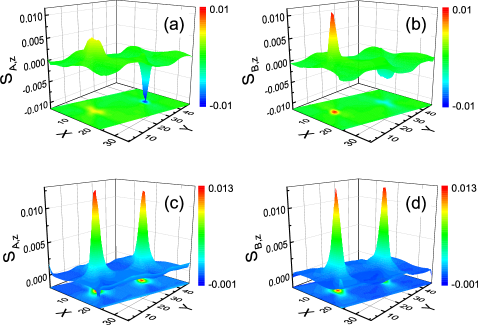
Figure 3: The spatial distributions of the induced magnetic orders in the vortex states with the magnetic field along the $-z$ direction for $\beta=0.04$ on sublattice $A$ (a), and on sublattice $B$ (b), respectively. (c) and (d) show the calculated results fot the spatial distributions of the induced magnetic orders by replacing $H_{ISOC}$ with $H_{KM}$ [see text for details].

III.2 The splitting and shift of the finite-energy peaks for the spin-resolved LDOS

Next, we examine the energy dependence of the LDOS in the vortex states on the honeycomb lattice. The LDOS is defined as $N(\mathbf{R}_{i},E)=N_{\uparrow}(\mathbf{R}_{i},E)+N_{\downarrow}(\mathbf{R}_{i},E)$ with $N_{\uparrow}(\mathbf{R}_{i},E)=-\sum_{n}|u_{A(B),n,i,\uparrow}|^{2}f^{\prime}(E_{n}-E)$ and $N_{\downarrow}(\mathbf{R}_{i},E)=-|v_{A(B),n,i,\downarrow}|^{2}f^{\prime}(E_{n}+E)$ being the spin-resolved LDOS for spin-up and spin-down states, respectively. In order to reduce the finite size effect, the calculations of the LDOS are carried out on a periodic lattice which consists of $16\times 8$ parallelogram vortex unit cells, with each vortex unit cell being the size of $24\mathbf{a_{1}}\times 48\mathbf{a_{2}}$. In Fig. 4, we plot a series of the spin-resolved LDOS as a function of energy at sites along the zigzag direction moving away from the vortex center for $\beta=0.0$ and $\beta=0.04$, respectively. For comparison, we have also displayed the LDOS at the midpoint between the two NN vortices, which resembles the U-shaped full gap feature for the bulk system. In the absence of ISOC, the states of spin-up and spin-down are nearly equal occupation and empty in the vortex core, as shown in Fig. 4(a), in accordance with the empty cores without the induced magnetic orders. Besides the almost identical LDOS line shapes for the spin-up and spin-down states, the LDOS shown in Fig. 4(a) exhibits another two prominent features within the SC gap edges. On one hand, the LDOS shows the pronounced discrete energy peaks inside the core region with one located near the zero energy and others located at finite energies, as indicated by the dashed vertical lines in the figure. Here, the asymmetric line shape of the LDOS with respect to zero energy reflects the lack of particle-hole symmetry as the chemical potential $\mu$ deviates from zero for the filling factor $n$ being greater than the half filling ($n>1$). Due to the particle-hole asymmetry, the finite-energy bound states at the core site only appear on the $E>0$ side Haya1 (There are also weak peaks at finite energies on the $E<0$ side when moving away from the core center.). The existence of the zero-energy vortex core sates in the Dirac fermion system have been predicted analytically by Jackiw and Rossi in terms of the zero-energy solutions of relativistic field theory Jack1 . Although these zero-energy solutions were subsequently demonstrated that the existence of these zero-energy solutions is connected to an index theorem Wein1 and the zero modes were shown to exist in the Dirac continuum theory of the honeycomb lattice at half filling Ghaemi1 , the zero-energy levels split when adopting a honeycomb lattice model description by setting the size of the vortex core to be zero Doro1 . It is also found that the energy splitting decreases with the vortex size and leads to the near-zero-energy states in the circumstance of finite core size Doro1 . While the notion of the zero-energy vortex core states presents an important subject of study being worthy of further research, we identify the near-zero-energy vortex core states here in a self-consistent manner by employing the honeycomb lattice model, where the band structure has the Dirac-type dispersion near the half filling. On the other hand, though the peaks’ intensities are suppressed as the site departing from the core center, the energy levels of these peaks are almost independent of positions. It is worth while to note that a dispersionless zero-energy conductance peak has been recently observed inside the SC vortex core by Chen’s group Liang1 in the kagome superconductor CsV₃Sb₅, which shares the lattice structure with component of hexagonal honeycomb and the electronic structure with Dirac points in a manner similar to those in honeycomb lattices. How the calculated results with near-zero-energy peaks in the present study relate to the experimental observations, and whether these near-zero-energy vortex core states have a common underlying symmetrical cause, constituting another fascinating questions deserving further studies.

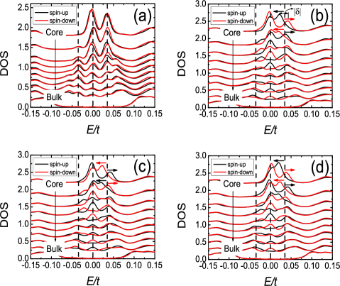
Figure 4: The energy dependence of the spin-resolved LDOS on a series of sites for $\beta=0.0$ (a), and for $\beta=0.04$ (b), (c) and (d). (a), (b) and (d) are the results for a magnetic field along the $z$-direction, while (c) the results for a magnetic field along the $-z$-direction. (b) and (c) show the LDOS inside the same vortex core, and (d) the LDOS inside another vortex core. In each panel from top to bottom, the curves stand for the LDOS at sites along the zigzag direction moving away from the core center. The curves are vertically shifted for clarity. The three dashed vertical lines in each panel denote the three low energy peak positions for $\beta=0$. The arrows in (b), (c) and (d) indicate the peak position shift with respect to that of $\beta=0$. The magnitude of the relative energy shifts $|\delta|$ is shown in (b).

In the presence of the ISOC, the local breaking of the spin and sublattice degeneracies in the vortex states is also reflected in the energy dependence of the LDOS. Figs. 4(b), 4(c) and 4(d) present the typical results of the spin-resolved LDOS for $\beta=0.04$. As can be seen from Fig. 4(b), while the energy level of the near-zero-energy peaks remain virtually unchanged for both spins, the energy levels of the finite-energy peaks are shifted differently by the ISOC for different spins and at different sublattice sites, as compared with the case of $\beta=0$. Specifically, for the LDOS on the same site within the core region, the finite-energy peaks for the spin-up and spin-down bound states shift oppositely, as indicated by the arrows in the figures, depicting a picture of local breaking of the spin degeneracy. At the same time, for the bound states with the same spin, the finite-energy peaks on the sites belonging to different sublattices also have the opposite shifts, indicating the local breaking of the sublattice degeneracy. Since there are induced magnetic orders in the vortex cores as well as the similar ISOC dependencies of the magnitudes of the magnetic orders $|S|_{max}$ and the relative energy shifts $|\delta|$ as shown in Fig. 1(d), it is natural to suspect whether the spin splitting for the LDOS is derived from the Zeeman effect of the induced local magnetic order interacting with the electrons Zhu2 , or from the above scenario where the spin degree of freedom is manipulated by the orbital effect of magnetic field via the ISOC. Several aspects render the Zeeman effect mechanism impossible. As has been shown in Fig. 2(b), the magnetic orders polarize oppositely inside two NN vortices. If the Zeeman effect mechanism runs, the energy level shifts of the peaks should behave the opposite way on the sites located respectively at the two NN vortices. Nevertheless, as displayed in Figs. 4(b) and 4(d), the consistency of the peaks’ shifts on the sites located at different vortices while belonging to the same sublattice rules out the Zeeman effect mechanism. The second thing we notice about the energy level shifts of the peaks is that they occur only for the ones with finite energy, while the near-zero-energy peaks almost stay the same, being at odds with the Zeeman effect mechanism. Finally, if we reverse the direction of the out-of-plane magnetic field, as shown in Fig. 4(c), the peaks’ shifts behave exactly the opposite way as compared with that in Fig. 4(b). It is thus confirmed that the local spin splitting and the local breaking of sublattice degeneracy are conformed with the above scenario where the spin degree of freedom is manipulated by the orbital effect of magnetic field via the ISOC in the SC vortex states.

Figure 5: Temperature (a), and magnetic field (b) evolutions of the maximum of the absolute value for the induced magnetic orders at vortex cores with $\beta=0.04$.

III.3 The effects of temperature and magnetic field strength on the induced orders

Due to the 2D nature of the Ising superconductors, the thermal effect on the induced magnetic orders constitutes an inevitable issue from both theoretical perspective and experimental realization. Although the system under study is 2D, the induced magnetic orders are formed under the combined actions of the magnetic field, the ISOC and the SC order, so they are not spontaneous ones. Meanwhile, the induced magnetic orders are localized inside the vortex core regions, and thus they are local ones. As a result, one may expect a different manner of the thermal effect on the induced magnetic orders as compared with the Mermin-Wagner theorem Mermin1 . To see the thermal effect on the induced magnetic orders, we calculate the temperature dependence of the magnitude of the magnetic orders. Fig. 5(a) shows the temperature dependence of the maximum of the absolute value for the induced magnetic order at the vortex core, where $T$ is rescaled by $T_{c}\approx 0.05$. As can be seen from the figure, the magnitude of the magnetic orders remains approximately constant at low temperature $T\leq 0.02T_{c}$ [see inset of Fig. 5(a)] as a result of the small thermal excitations and the almost unchanged vortex core size at this temperature regime Miller1 . After then it shows a steady decreasing trend with increasing temperature, and finally reaches a tiny value at $T\sim 0.5T_{c}$. The decreasing trend is mainly ascribed to the enlarging vortex core size with temperature Miller1 , the so-called Kramer-Pesch Effect Kramer1 . The enlarged vortex core would involve more different sublattice sites into the vortex core center, resulting in the reduction of the induced magnetic orders. Though the magnetic orders reduce their magnitude upon the increasing of the temperature, they sustain to a finite temperature. Therefore, one may expect to observe the induced magnetic orders under temperatures well below the SC critical temperature.

Another important factor to be considered in observing the induced magnetic orders is how the strength of the external magnetic field affects the induced magnetic orders. Since one vortex unit cell accommodates two vortices in the calculations, we have $B=2\Phi_{0}/A\sim 1/N$ with $A$ and $N$ being the area and the site number of the vortex unit cell. Fig. 5(b) displays the variation of the maximum of the absolute value for the induced magnetic orders with respect to different strengths of the magnetic field, which are realized in the calculations by varying the size of the parallelogram vortex unit cell. In the weak to moderate magnetic field region, there is little interference between the vortex cores due to the large inter-vortex spacing $d$. The increase of the magnetic field leads to more broken Cooper pairs inside the vortex cores to contribute to the formation of the magnetic orders, so the magnitude of the induced magnetic orders increases with the magnetic field strength, as evidenced in Fig. 5(b). However, as the magnetic field increasing further, the adjacent vortex cores with opposite polarizations of the induced magnetic order would get close enough (with a length scale being less than two times of the penetration depth $\lambda$) to interfere with one another, leading to the reduction of the magnitude of the magnetic order. This suggests the induced magnetic orders will be altered in an Abrikosov vortex lattice Abrik1 . On one hand, the formation of the Bloch wave Franz1 or the interactions among vortices Blatter1 in the vortex lattice will suppress the induced magnetic orders. On the other hand, since there are many vortices in the sample instead of just two, the polarization of the induced orders is not necessarily opposite for two adjacent vortex cores. Nevertheless, the result also means the induced magnetic orders would survive in the vortex lattice under a weak to moderate magnetic field as long as $d\gg\lambda$, i.e., the inter-vortex spacing is much larger than the penetration depth.

IV remarks and conclusion

The local magnetic orders induced in the SC vortex states have been extensively investigated on the cuprates superconductors Ogata1 ; Zhu2 ; Zhu3 ; Chen1 ; Taki1 ; Tsuch1 , where the emergence of the magnetic orders inside the core region was generally believed to be originated from the electrons’ correlations. These correlations usually come from the Coulomb interactions between electrons and that the induced magnetic orders have nothing to do with the chirality of the electrons. However, the induced local magnetic orders inside the SC vortex core by the ISOC has a direct bearing on what the electrons’ chirality is. As has been demonstrated that the amplitudes of the induced magnetic orders and the unusual energy shifts of the in-gap state peaks present here are related to the ISOC strength $\beta$, while their directions are determined by the direction of the magnetic field. The amplitude and the different polar direction of the induced local magnetic orders could be measured by the muon spin rotation ($\mu$SR) spectroscopy and the nuclear magnetic resonance experiments, and the energy shifts of the in-gap state peaks on different sublattice for different spins could be observed in the spin-polarized scanning tunneling microscopy experiments. Both of these observations may be served as signatures to characterize the ISOC proposed for the Ising superconductors. In the meantime, since the induced magnetic orders are derived from the ISOC, the breaking of the spin degeneracy and the energy shifts of the in-gap state peaks are selectively occurred for the electrons which possess finite momentum with respect to the vortex center. The scenario proposed here may also provide a possibility in manipulation of electron spins in motion via the orbital effect in the SC vortex states.

In conclusion, we have numerically investigated the vortex states of the Ising superconductors, with the emphasis on the local breaking of the spin and sublattice degeneracies as a result of the interaction between the ISOC derived effective fluxes and the local magnetic flux inside the vortex core. In the absence of the ISOC, there was no magnetic order induced inside the vortex core, and the almost identical line shapes of the LDOS for the spin-up and spin-down in-gap states were shown up inside the core region, forming a series of discrete energy peaks within the gap edges. The inclusion of the ISOC induced the ferromagnetic orders inside the vortex core region, where the magnetic orders polarized oppositely for the two NN vortices with one of the two polarizations coming dominantly from one specie of the two sublattices. Accordingly, the finite-energy peaks of the LDOS on the same site for spin-up and spin-down in-gap states were shifted oppositely by the ISOC, and the relative shifts of them on sublattices $A$ and $B$ were also of opposite algebraic sign. The calculated results might serve as experimental signatures for identifying the ISOC in the Ising superconductors, and the scenario proposed here might also be prospective in manipulation of electron spins in motion through the orbital effect in the SC vortex states.

V acknowledgement

This work was supported by the National Natural Science Foundation of China (Grant Nos. 11574069 and 61504035) and the Natural Science Foundation of Zhejiang Province (No. LY16A040010). This work was also supported by K. C. Wong Magna Foundation in Ningbo University.

References

- (1) R. A. Bromley, R. B. Murray, and A. D. Yoffe, J. Phys. C 5, 759 (1972).
- (2) Th. Böker, R. Severin, A. Müller, C. Janowitz, R. Manzke, D. Voß, P. Krüger, A. Mazur, and J. Pollmann, Phys. Rev. B 64, 235305 (2001).
- (3) Z. Y. Zhu, Y. C. Cheng, and U. Schwingenschlögl, Phys. Rev. B 84, 153402 (2011).
- (4) D. Xiao, G.-B. Liu, W. Feng, X. Xu, and W. Yao, Phys. Rev. Lett. 108, 196802 (2012).
- (5) J. T. Ye, Y. J. Zhang, R. Akashi, M. S. Bahramy, R. Arita, and Y. Iwasa, Science 338, 1193 (2012).
- (6) K. Taniguchi, A. Matsumoto, H. Shimotani, and H. Takagi, Appl. Phys. Lett. 101, 042603 (2012).
- (7) A. Kormányos, V. Zólyomi, N. D. Drummond, P. Rakyta, G. Burkard, and V. I. Fal’ko, Phys. Rev. B 88, 045416 (2013).
- (8) F. Zahid, L. Liu, Y. Zhu, J. Wang, and H. Guo, AIP Adv. 3, 052111 (2013).
- (9) E. Cappelluti, R. Roldán, J. A. Silva-Guillén, P. Ordejón, and F. Guinea, Phys. Rev. B 88, 075409 (2013).
- (10) X. Xi, L. Zhao, Z. Wang, H. Berger, L. Forró, J. Shan, and K. F. Mak, Nat. Nanotechnol. 10, 765 (2015).
- (11) W. Shi, J. T. Ye, Y. Zhang, R. Suzuki, M. Yoshida, J. Miyazaki, N. Inoue, Y. Saito, and Y. Iwasa, Sci. Rep. 5, 12534 (2015).
- (12) J. M. Lu, O. Zheliuk, I. Leermakers, N. F. Q. Yuan, U. Zeitler, K. T. Law, and J. T. Ye, Science 350, 1353 (2015).
- (13) Y. Saito, Y. Nakamura, M. S. Bahramy, Y. Kohama, J. Ye, Y. Kasahara, Y. Nakagawa, M. Onga, M. Tokunaga, T. Nojima, Y. Yanase, and Y. Iwasa, Nat. Phys. 12, 144 (2016).
- (14) X. Xi, Z. Wang, W. Zhao, J.-H. Park, K. T. Law, H. Berger, L. Forró, J. Shan, and K. F. Mak, Nat. Phys. 12, 139 (2016).
- (15) B. T. Zhou, N. F. Q. Yuan, H.-L. Jiang, and K. T. Law, Phys. Rev. B 93, 180501(R) (2016).
- (16) G. Sharma and S. Tewari, Phys. Rev. B 94, 094515 (2016).
- (17) A. H. Castro Neto, F. Guinea, N. M. R. Peres, K. S. Novoselov, and A. K. Geim, Rev. Mod. Phys. 81, 109 (2009).
- (18) P. A. Frigeri, D. F. Agterberg, A. Koga, and M. Sigrist, Phys. Rev. Lett. 92 097001 (2004).
- (19) B. Radisavljevic, A. Radenovic, J. Brivio, V. Giacometti, and A. Kis, Nat. Nanotechnol. 6, 147 (2011).
- (20) Y. J. Zhang, J. T. Ye, Y. Matsuhashi, and Y. Iwasa, Nano Lett. 12, 1136 (2012).
- (21) Q. H. Wang, K. Kalantar-Zadeh, A. Kis, J. N. Coleman, and M. S. Strano, Nat. Nanotechnol. 7, 699 (2012).
- (22) W. Bao, X. Cai, D. Kim, K. Sridhara, and M. S. Fuhrer, Appl. Phys. Lett. 102, 042104 (2013).
- (23) J. Lee, K. F. Mak, and J. Shan, Nat. Nanotechnol. 11, 421 (2016).
- (24) H.-M. Jiang, J.-L. Shang, and L.-Z. Hu, J. Phys.: Condens. Matter 31, 295602 (2019).
- (25) V. G. Kogan and N. V. Zhelezina, Phys. Rev. B 71, 134505 (2005).
- (26) A. Fente, E. Herrera, I. Guillamón, H. Suderow, S. Mañas-Valero, M. Galbiati, E. Coronado, and V. G. Kogan, Phys. Rev. B 94, 014517 (2016).
- (27) C. L. Kane and E. J. Mele, Phys. Rev. Lett. 95, 226801 (2005).
- (28) N. Hayashi, T. Isoshima, M. Ichioka, and K. Machida, Phys. Rev. Lett. 80, 2921 (1998).
- (29) R. Jackiw and P. Rossi, Nucl. Phys. B 190, 681 (1981).
- (30) E. J. Weinberg, Phys. Rev. D 24, 2669 (1981).
- (31) P. Ghaemi and F. Wilczek, Phys. Scr. T146, 014019 (2012).
- (32) D. L. Bergman and K. Le Hur, Phys. Rev. B, 79, 184520 (2009).
- (33) Z. Liang, X. Hou, F. Zhang, W. Ma, P. Wu, Z. Zhang, F. Yu, J.-J. Ying, K. Jiang, L. Shan, Z. Wang, and X.-H. Chen, Phys. Rev. X 11, 031026 (2021).
- (34) J.-X. Zhu and C. S. Ting, Phys. Rev. Lett. 87, 147002 (2001).
- (35) N. D. Mermin and H. Wagner, Phys. Rev. Lett. 17, 1133 (1966).
- (36) R. I. Miller, R. F. Kiefl, J. H. Brewer, J. Chakhalian, S. Dunsiger, G. D. Morris, J. E. Sonier, and W. A. MacFarlane, Phys. Rev. Lett. 85, 1540 (2000).
- (37) L. Kramer and W. Pesch, Z. Phys. 269, 59 (1974).
- (38) A. A. Abrikosov, Rev. Mod. Phys, 76, 975 (2004).
- (39) M. Franz and Z. Tešanović, Phys. Rev. Lett. 84, 554 (2000).
- (40) G. Blatter and V. Geshkenbein, Phys. Rev. Lett. 77, 4958 (1996).
- (41) M. Ogata, Int. J. Mod. Phys. B 13, 3560 (1999).
- (42) J.-X. Zhu, I. Martin, and A. R. Bishop, Phys. Rev. Lett. 89, 067003 (2002).
- (43) Y. Chen, Z. D. Wang, J.-X. Zhu, and C. S. Ting, Phys. Rev. Lett. 89, 217001 (2002).
- (44) M. Takigawa, M. Ichioka, and K. Machida, Phys. Rev. Lett. 90, 047001 (2003).
- (45) H. Tsuchiura, M. Ogata, Y. Tanaka, and S. Kashiwaya, Phys. Rev. B 68, 012509 (2003).