A Viral Marketing-Based Model For Opinion Dynamics in Online Social Networks

Abstract

Online social networks provide a medium for citizens to form opinions on different societal issues, and a forum for public discussion. They also expose users to viral content, such as breaking news articles. In this paper, we study the interplay between these two aspects: opinion formation and information cascades in online social networks. We present a new model that allows us to quantify how users change their opinion as they are exposed to viral content. Our model is a combination of the popular Friedkin–Johnsen model for opinion dynamics and the independent cascade model for information propagation. We present algorithms for simulating our model, and we provide approximation algorithms for optimizing certain network indices, such as the sum of user opinions or the disagreement–controversy index; our approach can be used to obtain insights into how much viral content can increase these indices in online social networks. Finally, we evaluate our model on real-world datasets. We show experimentally that marketing campaigns and polarizing contents have vastly different effects on the network: while the former have only limited effect on the polarization in the network, the latter can increase the polarization up to 59% even when only 0.5% of the users start sharing a polarizing content. We believe that this finding sheds some light into the growing segregation in today’s online media.

1 Introduction

Online social networks are a ubiquitous part of modern societies. In addition to connecting users with their friends, many people also use them as content aggregators, by following media outlets or reading articles shared by their peers. Clearly, engaging in social networks may impact one’s opinions with respect to societal issues: users might adjust their opinions during a discussion based on arguments by their peers; or they might adapt their opinions based on new facts revealed in a news article they read.

Due to this strong connection between opinion formation and information spread, online social networks have become the target of viral disinformation campaigns. Popular examples include groups like QAnon who spread conspiracy theories and fake news about topics, such as vaccination, or state actors who try to influence election results in opposing countries. While it is well-researched how viral content spreads through social networks, such models do not consider how user opinions are impacted by the viral content. Therefore, understanding how new information influences user opinions and being able to quantify the impact of such disinformation campaigns is highly desirable.

A prominent model to quantify opinion dynamics in social networks is the Friedkin–Johnsen (FJ) model [18]. The FJ model stipulates that each user has an expressed opinion that the user reveals publicly and is network-dependent, and an innate opinion that is fixed and network-independent. However, it does not take into account how users change their opinions based on new information (e.g., viral content) that is disseminated in the network.

Furthermore, researchers have studied problems related to optimizing certain opinion-based network indices, for instance, maximizing the average opinion [20] or polarization [10, 19], or minimizing polarization and disagreement [12, 29, 32]. In this line of work, optimization occurs by nudging the expressed or innate opinions of a set of seed users towards a certain direction. However, existing works do not specify how such nudging takes place, nor do they consider the interplay of opinion nudging within a more realistic setting of information cascades.

Therefore, the current research either allows us to quantify user opinions and optimize opinion-based network indices without taking into account viral content or it allows to assess the spread of viral content without reasoning about user opinions. This limitation leads us to the following questions:

1. Can we quantify how viral content influences user opinions in online social networks?

2. Can we study the interplay between information cascades and opinion dynamics?

3. Can we optimize opinion-based network indices by taking into account the spread of viral content?

Our contributions. We answer the above questions affirmatively by proposing a new model that combines the Friedkin–Johnsen model [18] and the influence-maximization framework of Kempe et al. [25]. To the best of our knowledge, our model is the first that allows to quantify the impact of viral content on user opinions.

Contrasted with the vanilla FJ model in which the innate user opinions are “fixed” but the expressed opinions are changing over time based on user interactions, our model considers the viral content that is shared in the network, and it assumes that for users who are exposed to this content, there is a probability that their innate opinion changes. This could be the case, for example, when a user reads an article that makes them reconsider their stance on a certain topic.

When a subset of users change their innate opinions, their expressed opinions will also be modified, which in turn will have an impact on the whole network via the FJ opinion dynamics. Thus, the change of the innate opinions of few users may have an impact on the whole network: even when a user’s innate opinion does not change by the viral content (because they ignore it or the content never reaches them), they still might change their expressed opinion due to “peer-pressure.”

Our model connects these two phenomena: it allows us to understand how viral content can impact individual users, while it also enables us to study how individual behavior ripples through the network and affects the overall discussion.

We consider two different types of content: non-polarizing and polarizing. For non-polarizing content, such as marketing campaigns, the innate opinions of the users can only increase. For polarizing content, we take into account the backfire effect [33]: interaction with opposing content may lead to a decrease in a user’s innate opinion. This could be the case, e.g., in political campaigns when a party runs an ad that makes their supporters react positively but their opponents react negatively.

From an algorithmic view point, we present methods for simulating our model. Additionally, we consider the problem of optimizing certain opinion-based network indices. We present a greedy $(1-1/e-\epsilon)$-approximation algorithm for maximizing the sum of user opinions for non-polarizing content. We also present algorithms for maximizing the controversy and the disagreement–controversy indices [32] for non-polarizing content; our algorithms have data-dependent approximation ratios. Finally, we provide heuristics for maximizing other indices, such as polarization and disagreement, for non-polarizing and polarizing content.

To obtain our optimization algorithms, we build upon the reverse-reachable sets framework [7, 37, 36]. One challenge is that, in our setting, the arising optimization problems are based on quadratic forms and, therefore, we have to extend the reverse reachable set framework to this more general setting.

We evaluate our methods on real-world data. Our experiments reveal a striking difference between non-polarizing and polarizing content. On the one hand, non-polarizing content can significantly increase the sum of user opinions, but it has limited impact on the polarization and sometimes even decreases it. The situation for polarizing content is the opposite: it barely increases the sum of user opinions but it can increase the polarization significantly. We see that even when only 0.5% of the users start sharing a polarizing content, the network polarization increases by more than 20% on average and can rise up to 59%. We believe that this finding provides an explanation for the growing polarization that can be witnessed in modern day’s online media.

We present the proofs of our claims in the appendix.

2 Related work

Our aim is to quantify how viral content impacts user opinions in social networks. Naturally, our approach builds on existing models for opinion dynamics and information cascades.

Opinion dynamics have been studied in different research areas, including psychology, social sciences, and economics [8, 24]. Here we build on the popular Friedkin–Johnsen (FJ) model [18], which is an extension of a classic model by DeGroot [17]. Many extensions of the FJ model have been proposed. For example, Amelkin et al. [1] assume that the innate user opinions change over time based on the expressed opinions. We refer to the discussion in [1] for other related models. However, these works do not take into account the changes of innate opinions based on exposition to viral contents.

Recent work used these models for understanding properties of opinion dynamics and formulating natural optimization problems. Bindel et al. [6] analyze the “price of anarchy” in the FJ model by considering as cost the internal conflict of the individuals in the network and comparing the cost at equilibrium and the social optimum. Gionis et al. [20] maximize the sum of opinions of the network users. Other works study the problem of measuring and reducing polarization of opinions, or other disagreement indices, in the FJ model [14, 29, 32, 40], while adversarial settings have also been considered, aiming to quantify the power of an adversary seeking to induce discord in the model [12, 10, 19].

To model information cascades, we build on the popular independent-cascade model of Kempe et al. [25]. Many extensions and variants of this model have been proposed. For example, Sathanur et al. [35] incorporate intrinsic user activations based on external sources. Another popular extension is the topic-aware cascade model by Barbieri et al. [5], and has various applications including social advertising [3, 2]. While such models allow to model information spread, they do not allow to quantify how these change the user opinions.

The backfire effect, the tendency of individuals to hold firmly on their beliefs when faced with factual corrections, has been observed in political sciences [33], but has not been studied extensively in computational social sciences. Exceptions are the works of Chen et al. [13], who incorporate backfire in an opinion-dynamics model for biased assimilation [16], and Hirakura et al. [22], who propose a model of polarization that incorporates empathy and repulsion.

Our optimization algorithms rely on reverse reachable sets, introduced by Borgs et al. [7], and improved by subsequent techniques [37, 36]. We extend these ideas to our setting, to obtain algorithms for objectives that include quadratic terms. We note that the activity-maximization task defined by Wang et al. [38] is a special case of our setting. We apply the “sandwich” framework [28] to obtain data-dependent approximation guarantees for some of our objectives. For the efficient computation of our objective functions, we use the methods by Xu et al. [39] based on Laplacian solvers.

To our knowledge, this is the first work that studies how user opinions change due to viral information in online social networks. For fixed user opinions, Monti et al. [31] studied how cascades spread through the network, based on the user opinions and the topics of the contents.

3 Preliminaries

Let $G=(V,E,w)$ be an undirected weighted graph, with $n=\lvert V\rvert$ nodes and edge weights $w\colon E\rightarrow\mathbb{R}_{>0}$. We let $N(u)$ denote the set of neighbors of $u\in V$. The Laplacian of $G$ is $\mathbf{L}=\mathbf{D}-\mathbf{W}$, where $\mathbf{D}$ is the $n\times n$ diagonal matrix with $\mathbf{D}_{u,u}=\sum_{v\in N(u)}w(u,v)$ for all $u\in V$ and $\mathbf{W}$ is the $n\times n$ matrix with $\mathbf{W}_{u,v}=w_{u,v}$ for all $u,v\in V$.

Friedkin–Johnsen (FJ) model. In the FJ model, we are given a weighted undirected graph $G=(V,E,w)$ with $n$ nodes. Each node $u$ corresponds to a user of a social network. Each user $u$ has an expressed opinion $z_{u}\in[0,1]$, which depends on the network, and a fixed innate opinion $s_{u}\in[0,1]$. We write $\mathbf{s}\in[0,1]^{n}$ and $\mathbf{z}\in[0,1]^{n}$ to denote the vectors of innate and expressed opinions.

The expressed opinions are updated in rounds. More concretely, let $\mathbf{s}$ be the vector of innate opinions, and $\mathbf{z}^{(t)}$ be the vector of expressed opinions at time $t$. The update rule is given by

$$\mathbf{z}^{(t+1)}=(\mathbf{D}+\mathbf{I})^{-1}(\mathbf{W}\mathbf{z}^{(t)}+\mathbf{s}).$$ (3.1)

Taking the limit $t\rightarrow\infty$, the expressed opinions converge to

$$\mathbf{z}^{*}=(\mathbf{I}+\mathbf{L})^{-1}\mathbf{s}.$$ (3.2)

Table 1: Matrices of the different indices.

Index	Notation	Matrix
Polarization	${\mathcal{P}}(\mathbf{L})\,$	$(\mathbf{I}+\mathbf{L})^{-1}(\mathbf{I}-\frac{\mathbf{1}\mathbf{1}^{\intercal}}{n})(\mathbf{I}+\mathbf{L})^{-1}$
Disagreement	${\mathcal{D}}(\mathbf{L})\,$	$(\mathbf{L}+\mathbf{I})^{-1}\mathbf{L}(\mathbf{L}+\mathbf{I})^{-1}$
Internal conflict	${\mathcal{I}}(\mathbf{L})\,$	$(\mathbf{L}+\mathbf{I})^{-1}\mathbf{L}^{2}(\mathbf{L}+\mathbf{I})^{-1}$
Controversy	${\mathcal{C}}(\mathbf{L})\,$	$(\mathbf{L}+\mathbf{I})^{-2}$
Disagreement–controversy	${\mathcal{I}^{\mathit{dc}}}(\mathbf{L})\,$	$(\mathbf{L}+\mathbf{I})^{-1}$

We study the following popular network indices in our model, where the matrices of the quadratic forms are as defined in Table 1:

• sum of user opinions, which is given by $\mathcal{S}_{\mathbf{s}}=\mathbf{1}^{\intercal}\mathbf{s}$, and it is well-known that $\mathcal{S}_{\mathbf{s}}=\mathbf{1}^{\intercal}\mathbf{z}$;

• polarization [32] $\mathcal{P}_{G,\mathbf{s}}=\sum_{u\in V}(z_{u}^{*}-\bar{\mathbf{z}})^{2}=\mathbf{s}^{\intercal}{\mathcal{P}}(\mathbf{L})\,\mathbf{s}$, where $\bar{\mathbf{z}}=\frac{1}{n}\sum_{u\in V}z_{u}^{*}$ is the average user opinion;

• disagreement [32] $\mathcal{D}_{G,\mathbf{s}}=\sum_{(u,v)\in E}w_{u,v}(z_{u}^{*}-z_{v}^{*})^{2}=\mathbf{s}^{\intercal}{\mathcal{D}}(\mathbf{L})\,\mathbf{s}$;

• internal conflict [12] $\mathcal{I}_{G,\mathbf{s}}=\sum_{u\in V}(s_{u}-z_{u}^{*})^{2}=\mathbf{s}^{\intercal}{\mathcal{I}}(\mathbf{L})\,\mathbf{s}$;

• controversy [12, 29] $\mathcal{C}_{G,\mathbf{s}}=\sum_{u\in V}(z_{u}^{*})^{2}=\mathbf{s}^{\intercal}{\mathcal{C}}(\mathbf{L})\,\mathbf{s}$; and

• disagreement-controversy [39, 32]​ $\mathcal{I}^{\mathit{dc}}_{G,\mathbf{s}}\!=\!\mathbf{s}^{\intercal}{\mathcal{I}^{\mathit{dc}}}(\mathbf{L})\,\mathbf{s}\!=\!\mathcal{C}_{G,\mathbf{s}}\!+\!\mathcal{D}_{G,\mathbf{s}}$.

4 Modelling the Influence of Viral Content on User Opinions

We formally introduce our model in Sec. 4.1 and show how it can be simulated in Sec. 4.2.

4.1 The spread-acknowledge model

Following the independent cascade model [25], we assume that a value $p_{u,v}\in[0,1]$ encodes the probability that user $v$ reacts to content received from user $u$; we allow that $p_{u,v}\neq p_{v,u}$. Furthermore, we introduce parameters $\epsilon,\delta>0$, as explained below.

As per the FJ model, each user $u$ has an expressed opinion $z_{u}$ and an innate opinion $s_{u}$. Additionally, each user has a state, which is either inactive, ignore, acknowledge or spread. We order the states by “inactive $<$ ignore $<$ acknowledge $<$ spread” and we follow the convention that when a user changes their state, they can only pick one that is higher with respect to this ordering. An illustration of the model with respect to state transitioning and actions performed for a single node $v$ is provided in Figure 1.

Our model proceeds in rounds. Initially, in round $0$, there are $k$ users whose state is spread and all other users are inactive; in later rounds, it is possible that users change their state. We will refer to the users whose initial state is spread as seed nodes. Each round $t>0$ has two phases: In the first phase, the users update their expressed opinions. In the second phase, the viral content is spread through the network and users may change their state and their innate opinion. We describe both phases below.

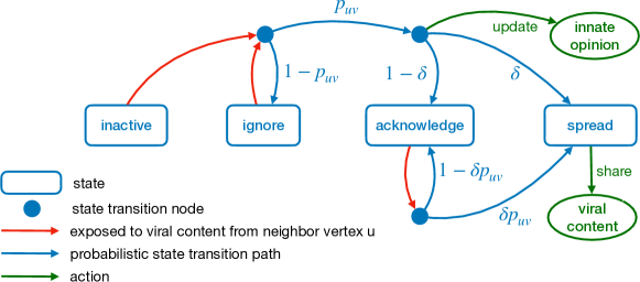
Figure 1: An illustration of the spread-acknowledge model with respect to state transitioning and actions performed for a single node $v$. In the initial round, $k$ seed nodes are in state spread, while the rest of nodes are in state inactive.

Phase I: Updating user opinions. The users update their expressed opinion as in the FJ model, i.e., according Eq. (3.1).

Phase II: Information spreading. Consider round $t>0$. Let $U$ denote the set of users who have changed their state to spread in round $t-1$. If $U=\emptyset$, we consider Phase II finished. Otherwise ($U\neq\emptyset$), each user $u\in U$ shares the viral content with all of its neighbors. When a neighbor $v$ of $u$ is exposed to the viral content, it switches to a new state and possibly adjusts its innate opinion. If $v$ is in state inactive or ignore, then this is done as follows:

• With probability $\delta p_{uv}$, user $v$ switches to state spread; $v$ adjusts its innate opinion (described below) and shares the content in the next round with its neighbors.

• With probability $(1-\delta)p_{uv}$, user $v$ switches to state acknowledge; $v$ adjusts its innate opinion (described below) but does not share the content with its neighbors in the next round.

• With probability $1-p_{uv}$, user $v$ switches to state ignore; $v$ performs no action (i.e., $v$ does not try to share the content and $v$ also does not adjust its innate opinion).

If $v$ is in state acknowledge then it switches to state spread with probability $\delta p_{uv}$ and remains in state acknowledge with probability $1-\delta p_{uv}$. Finally, if $v$ is in state spread then $v$ always stays in this state. In both of these cases, $v$ does not adjust its opinion again.

The above process ensures that the state ordering defined before is obeyed during state switching and that each user adjusts its innate opinion at most once. Finally, note that our model is a generalization of the independent cascade model if $\delta=1$.

Adjusting innate opinions. Now we describe how users change their innate opinions when they are exposed to viral content.

Consider user $u$ at state inactive or ignore whose new state becomes acknowledge or spread. Then the innate opinion $\mathbf{s}_{u}$ changes to a new value $\hat{\mathbf{s}}_{u}$. We consider two scenarios:

• Marketing campaign: The user’s opinion becomes more positive after seeing the content, i.e., $\hat{\mathbf{s}}_{u}=\min\{\mathbf{s}_{u}+\epsilon,1\}$ for the parameter $\epsilon>0$ from above. Here, we use the $\min$-operation to ensure that the new opinion $\hat{\mathbf{s}}_{u}$ is in the interval $[0,1]$.

• Polarizing campaign with backfire: In a polarizing campaign we assume that while some users embrace the content, others will find it repelling. More concretely, we assume that there is a threshold $\tau\in[0,1]$ such that: (1) If $\mathbf{s}_{u}\geq\tau$ then $u$ embraces the content and adjusts its opinion to $\hat{\mathbf{s}}_{u}=\min\{\mathbf{s}_{u}+\epsilon,1\}$; (2) If $\mathbf{s}_{u}<\tau$, then $u$ finds the content repelling and adjusts $\hat{\mathbf{s}}_{u}=\max\{0,\mathbf{s}_{u}-\epsilon\}$.

Note that in our model with polarizing campaigns, users can still share a content they dislike. While this might seem non-intuitive at first, we believe that it is a realistic behavior: users who oppose a certain content often share it together with a counter-argument. We remark that our model can be modified to avoid this.

Finally, observe that $\hat{\mathbf{s}}$ is a random vector that depends on the outcome of the information spread. However, once we fix the randomness of the information spread, $\hat{\mathbf{s}}$ becomes deterministic. This will be a useful property in the following.

Possible model extensions. We note that our model is quite general and can be extended in various ways. First, we modelled information cascades via the independent cascade model [25]. However, our model and our result from Lemma 4.1 also hold if we used the linear threshold model [25], topic-aware versions of the independent cascade and linear threshold models [5], as well as intrinsic user activations [35]. In particular, using the linear threshold model could lead to insights on contents that spread via complex contagion [9, 21]. Second, above we considered the two relatively simple settings for adjusting the innate user opinions $\hat{\mathbf{s}}_{u}$. However, we note that Lemma 4.1 below generalizes to the setting when $\hat{\mathbf{s}}_{u}$ is any user-defined function of $\mathbf{s}_{u}$.

4.2 Equivalence with the two-stage model

While the spread-acknowledge model is easy to explain and motivate by real-world scenarios, it is not clear how to simulate it efficiently. If we implemented the model as described above, we would have to update the expressed opinions in each round, which can be costly. To avoid this, we now introduce a new model that can be simulated more efficiently, and we show that it produces an identical distribution over the innate and expressed opinions.

The two-stage model. Our simplified model also proceeds in rounds, but it performs the information spreading and the updating of the user opinions in two sequential stages. More concretely, in each round of the first stage, we perform the information spreading process that is described in Phase II above (and we do not perform the updating of the expressed opinions as per Phase I). In this process, some of the users’ innate opinions and their states might change. When after a round no new users have changed their state to spread, we start the second stage. In each round of the second stage, we perform the same update of the expressed opinions as described in Phase I above (and we do not run Phase II).

Simulating the two-stage model. Next, we discuss why the two-stage model is well-suited for efficient simulations. First, observe that the first stage stops when no node changed their state to spread in the previous round, i.e., when $U=\emptyset$. Therefore, the first stage can have at most $O(n)$ rounds (since each of the $n$ users can take at most four different states and since we assumed that users only increase their state with respect to the ordering of the states). Additionally, in each round of the first stage, we can update the states of the nodes by iterating over all nodes $v$ that are neighbors of a node $u\in U$ and then updating the state of $v$ with the probability described in Phase II. Since each user can become a spreader only once, the time for executing all rounds of the first stage is $O(m)$, where $m$ is the number of edges in the graph.

Second, recall that the adjusted innate opinions $\hat{\mathbf{s}}_{u}$ only depend on the randomness from the information spreading process. Therefore, after the first stage finished, the innate opinions $\hat{\mathbf{s}}_{u}$ are fixed. Thus, we can assume that the vector $\hat{\mathbf{s}}_{u}$ is known and the expressed equilibrium opinions are given by $\hat{\mathbf{z}}^{*}=(I+L)^{-1}\hat{\mathbf{s}}$. The time complexity for the second stage is the time required to solve for $\hat{\mathbf{z}}^{*}$.

Equivalence of the opinion distributions. It remains to show that both models induce the same distribution over the innate and expressed opinions. To show this equivalence, we assume that both models are run with the same input graphs, the same seed nodes, and the same (non-adjusted) innate opinions $\mathbf{s}$. Now let us denote the adjusted innate opinions generated by the spread-acknowledge model by $\hat{\mathbf{s}}_{u}$ and those by the two-stage model by $\tilde{\mathbf{s}}_{u}$. Recall that both $\hat{\mathbf{s}}_{u}$ and $\tilde{\mathbf{s}}_{u}$ are random vectors that depend only on the outcome of the information-spreading process. The following lemma asserts the equivalence of the two models. The proof is presented in Appendix B.1.

Lemma 4.1.

For all $a\in[0,1]^{n}$, $\Pr[\hat{\mathbf{s}}=a]=\Pr[\tilde{\mathbf{s}}=a]$. Furthermore, let $\hat{\mathbf{z}}^{*}=(I+L)^{-1}\hat{\mathbf{s}}$ and $\tilde{\mathbf{z}}^{*}=(I+L)^{-1}\tilde{\mathbf{s}}$ be the equilibrium opinions. Then $\Pr[\hat{\mathbf{z}}^{*}=b]=\Pr[\tilde{\mathbf{z}}^{*}=b]$ for all $b\in[0,1]^{n}$.

5 Algorithms

We now present algorithms for maximizing the indices defined in Sec. 3. We start with algorithms for approximating the indices (Sec. 5.1). Then we present our algorithms for maximizing the sum of user opinions (Sec. 5.2) and for maximizing the controversy and the disagreement–controversy indices (Sec. 5.3). We present our proofs in Appendix B.

5.1 Estimating indices

Let ${\mathcal{M}}(\mathbf{L})\,$ be one of the matrices from Table 1, which induces the quadratic form for each of the indices that we wish to study. Recall that $\mathbf{s}$ is the non-adjusted vector of innate opinions and $\hat{\mathbf{s}}$ is the random vector of adjusted innate opinions. In the following, our goal is to compute $\mathbb{E}[\hat{\mathbf{s}}^{\intercal}{\mathcal{M}}(\mathbf{L})\,\hat{\mathbf{s}}]$.

Let $\Delta\hat{\mathbf{s}}=\hat{\mathbf{s}}-\mathbf{s}$ be the random vector that denotes how the users changed their opinions. Then observe that

$$\mathbb{E}[\hat{\mathbf{s}}^{\intercal}{\mathcal{M}}(\mathbf{L})\,\hat{\mathbf{s}}]=\mathbf{s}^{\intercal}{\mathcal{M}}(\mathbf{L})\,\mathbf{s}+\mathbb{E}[2\mathbf{s}^{\intercal}{\mathcal{M}}(\mathbf{L})\,\Delta\hat{\mathbf{s}}+\Delta\hat{\mathbf{s}}^{\intercal}{\mathcal{M}}(\mathbf{L})\,\Delta\hat{\mathbf{s}}].$$

Since the first term in the sum is deterministic, we drop it and focus on $\mathbb{E}[h(\Delta\hat{\mathbf{s}})]$, where $h(\Delta\hat{\mathbf{s}}):=2\mathbf{s}^{\intercal}{\mathcal{M}}(\mathbf{L})\,\Delta\hat{\mathbf{s}}+\Delta\hat{\mathbf{s}}^{\intercal}{\mathcal{M}}(\mathbf{L})\,\Delta\hat{\mathbf{s}}$. We show that computing $\mathbb{E}[h(\Delta\hat{\mathbf{s}})]$ is $\#\mathbf{P}$-hard since our model generalizes the independent cascade model.

Lemma 5.1.

Given seed nodes $S$, computing $\mathbb{E}[h(\Delta\hat{\mathbf{s}})]$ is $\#\mathbf{P}$-hard.

Monte Carlo Simulation. Since Lemma 5.1 shows that computing $\mathbb{E}[h(\Delta\hat{\mathbf{s}})]$ exactly is hard, we resort to approximations. One option is to use Monte Carlo simulations of our model. More concretely, we can simulate our model as described in Sec. 4.2 to obtain multiple samples of $\hat{\mathbf{s}}$. Now a Chernoff bound implies that we can compute an approximation of $\mathbb{E}[\hat{\mathbf{s}}]$ with high probability. Then we can compute an approximation of $\mathbb{E}[h(\Delta\hat{\mathbf{s}})]$ in near-linear time using the algorithms by Xu et al. [39], which are based on Laplacian solvers. This approach is efficient when the number of seed node sets for which we wish to compute $\mathbb{E}[h(\Delta\hat{\mathbf{s}})]$ is small.

Reverse reachable sets. However, in our optimization algorithms we will need to evaluate $\mathbb{E}[h(\Delta\hat{\mathbf{s}})]$ for a large number of different seed node sets and thus using the Monte Carlo approach is too inefficient. Therefore, we use reverse influence sampling [7, 37, 36], which allow us to reduce the number of simulations of our model.

Our notion of reverse reachable sets is as follows. Suppose that we want to simulate our model on a graph $G=(V,E)$. A possible world is a copy of $G$ that has labels on the edges and we generate the labels as follows. For each edge $(u,v)\in E$, we pretend that $u$ has state spread and $v$ has state inactive. Now we sample the state of $v$ as described in Phase II above and we label $(u,v)$ with the new state of $v$. For example, if $v$ changes its state to acknowledge then the label of $(u,v)$ is acknowledge. This process is repeated for all edges $(u,v)\in E$ and we always assume that $u$ has state spread and $v$ has state inactive, regardless of the outcomes of previous samples.

Now consider a possible world $g$. We say that there exists a live path from $u$ to $v$ if there exists a path in $g$ in which all edges have label spread except the edge incident upon $v$ which may have label acknowledge or spread. Notice that live paths encode when users change their opinions in our model: user $v$ adjusts its opinion if and only if there exists a live path from a seed node to $v$.

Next, let $g$ be a randomly generated possible world and let $u$ be a random node in $G$. A random rr-set $R$ for $u$ in $g$ is a set of nodes in $g$ such that there exists a live path to $u$.

Estimating indices. Now we turn to estimating $\mathbb{E}[h(\Delta\hat{\mathbf{s}})]$. Existing information propagation methods can be used for estimating $2\mathbb{E}[\mathbf{s}^{\intercal}{\mathcal{M}}(\mathbf{L})\,\Delta\hat{\mathbf{s}}]$, because $\Delta\hat{\mathbf{s}}$ is the only random quantity in this expression. However, we also need to approximate $\mathbb{E}[\Delta\hat{\mathbf{s}}^{\intercal}{\mathcal{M}}(\mathbf{L})\,\Delta\hat{\mathbf{s}}]=\sum_{u,v}{\mathcal{M}}(\mathbf{L})\,_{u,v}\mathbb{E}[\Delta\hat{\mathbf{s}}_{u}\Delta\hat{\mathbf{s}}_{v}]$, which involves products of random variables and which existing methods cannot do. Our main observation is that in each possible world it holds that $\Delta\hat{\mathbf{s}}_{u}\Delta\hat{\mathbf{s}}_{v}\neq 0$ if and only if there exist live paths from the seed nodes to $u$ and $v$. Wang et al. [38] followed a similar approach but only considered pairs $(u,v)$ for which there exist edges in the graph; here, we have to perform this operation for all pairs $(u,v)\in V^{2}$.

In the following, we set $\Delta s_{u}\in[-\epsilon,\epsilon]$ to denote how much user $u$ adjusts its opinion once it reaches state acknowledge or spread. Note that $\lvert\Delta s_{u}\rvert$ can be smaller than $\epsilon$ because of the interval concatenation that we described in Phase II above. Next, let $S$ be a set of seed nodes and let $\mathbf{1}_{u}(S)$ be an indicator with $\mathbf{1}_{u}(S)=1$ if $u$ adjusts innate opinion and otherwise $\mathbf{1}_{u}(S)=0$. Let $\mathbf{1}(S)$ be a vector of $\mathbf{1}_{u}(S)$ consisting of each $u\in V$. Note that $\mathbf{1}(S)$ is a random vector and that $\Delta\mathbf{s}$ is deterministic. Observe that $\Delta\hat{\mathbf{s}}=\Delta\mathbf{s}\odot\mathbf{1}(S)$, where is $\odot$ the Hadamard product.

To simplify our notation, we set $w_{u}=(2\mathbf{s}^{\intercal}{\mathcal{M}}(\mathbf{L})\,)_{u}\Delta s_{u}$ and let $m_{u,v}=(\Delta s_{u})^{\intercal}{\mathcal{M}}(\mathbf{L})\,_{u,v}\Delta s_{v}$. Then we obtain:

$$h(\Delta\hat{\mathbf{s}})=\sum_{u,v\in V}\frac{1}{n}w_{u}\mathbf{1}_{u}(S)+m_{u,v}\mathbf{1}_{u}(S)\mathbf{1}_{v}(S)=:F(S).$$

Given these definitions, we let $R_{u}$ and $R_{v}$ be random rr-sets for $u$ and $v$, respectively, and we set

$$\omega_{R_{u},R_{v}}(S)=\mathbbm{1}[(R_{u}\cap S)\neq\emptyset]w_{u}+\mathbbm{1}[(R_{u}\cap S)\neq\emptyset,(R_{v}\cap S)\neq\emptyset]n\,m_{u,v},$$

and for a set $\mathcal{R}$ of random rr-sets we define

$$F_{\mathcal{R}}(S)=\frac{\sum_{(R_{u},R_{v})\in\mathcal{R}}\omega_{R_{u},R_{v}}(S)}{\lvert\mathcal{R}\rvert}.$$ (5.1)

We show that $F_{\mathcal{R}}(S)$ is an unbiased estimator for $\mathbb{E}[F(S)]$.

Lemma 5.2.

Let $\mathcal{R}$ be a set of samples of pair of random rr-sets. Then $\mathbb{E}[F(S)]=\mathbb{E}_{u,g\sim\mathcal{G}}[n\,F_{\mathcal{R}}(S)]$.

Since the previous lemma only holds in expectation, we now consider approximations that hold with high probability. Let $\ell>0$ be an error parameter, $\theta=\lvert\mathcal{R}\rvert$ be the number of rr-sets and suppose we know ${\mathrm{OPT}}=\max_{\lvert S\rvert\leq k}\mathbb{E}[F(S)]$ (we show later how to obtain bounds on ${\mathrm{OPT}}$ using statistical tests). Our goal will be to pick $\theta$ large enough such that

$$\Pr[\lvert n\,F_{\mathcal{R}}(S)-\mathbb{E}[F(S)]\rvert\geq\frac{\epsilon}{2}\,{\mathrm{OPT}}]\leq\frac{1}{n^{\ell}\binom{n}{k}},$$ (5.2)

since then a union bound implies that for any seed set $S$ of size $k$, $\mathbb{E}[F(S)]$ is a good estimator for $F_{\mathcal{R}}(S)$ w.h.p. We show that if we pick $\theta$ large enough then Equation (5.2) is satisfied.

Lemma 5.3.

Let $\chi=\max_{u,v\in V}|w_{u}+n\,m_{u,v}|$ and $\lambda=\frac{8n\chi}{\epsilon^{2}}(\frac{\epsilon}{3}+1)(\ell\ln n+\ln 2+\ln\binom{n}{k})$. If $\theta\geq\frac{\lambda}{{\mathrm{OPT}}}$ then Equation (5.2) holds.

5.2 Maximizing network indices

Now we consider the sum of expressed opinions problem, where we are given an undirected weighted graph $G=(V,E)$ with edge probabilities $p_{u,v}$ and a positive integer $k$. The goal is to find a set of seed nodes of cardinality at most $k$ that maximizes the sum of expressed opinions $\mathbb{E}[\mathcal{S}_{\hat{\mathbf{s}}}]=\mathbb{E}[\mathbf{1}^{\intercal}\hat{\mathbf{z}}^{*}]$. Our main result is as follows.

Theorem 5.4.

There exists a greedy approximation algorithm that computes a $(1-1/e-\epsilon)$-approximation with high probability.

Indeed, in Appendix C we show that our model is strictly more powerful than the FJ model in which we can increase $k$ innate user opinions.

input : $\mathcal{R}$, $k$

output : $\tilde{X}^{G}$

$\tilde{X}^{G}\leftarrow\emptyset$

while $\lvert\tilde{X}^{G}\rvert\leq k$ do

       $x\leftarrow\arg\max_{x}F_{\mathcal{R}}(\tilde{X}^{G}\cup\{x\})-F_{\mathcal{R}}(\tilde{X}^{G})$;

       $\tilde{X}^{G}\leftarrow\tilde{X}^{G}\cup\{x\}$;

return $\tilde{X}^{G}$

Algorithm 1 $\mathrm{RR\text{-}Greedy}$

input : $\tilde{\mathbf{G}}$, $\lambda$, $\beta$, $\epsilon_{2}$, $k$, $\Delta\mathbf{s}$, $\chi$, $\mathrm{LB}_{0}$

output : $\mathcal{R}$

$\mathcal{R}\leftarrow\emptyset$, $\mathrm{LB}\leftarrow\mathrm{LB}_{0}$;

for $i=1,\ldots,\log_{2}n-1$ do

       $y\leftarrow n/2^{i}$, $\theta_{i}\leftarrow\frac{\beta}{y}$;

       while $\lvert\mathcal{R}\rvert\leq\theta_{i}$ do  $\mathcal{R}\leftarrow\mathcal{R}\cup\mathrm{GenerateRR\text{-}Set}$;

       $\tilde{\mathbf{X}}_{i}\leftarrow\mathrm{RR\text{-}Greedy}(\mathcal{R},k)$;

       if $n\,F_{\mathcal{R}}(\tilde{\mathbf{X}}_{i})\geq(1+\epsilon_{2})\,y\chi,$ then  $\mathrm{LB}\leftarrow\frac{n\,F_{\mathcal{R}}(\tilde{\mathbf{X}}_{i})}{1+\epsilon_{2}}$, break;

      

$\theta\leftarrow\lambda/\mathrm{LB}$;

while $\lvert\mathcal{R}\rvert\leq\theta$ do  $\mathcal{R}\leftarrow\mathcal{R}\cup\mathrm{GenerateRR\text{-}Set}$;

Return $\mathcal{R}$;

Algorithm 2 $\mathrm{Sampling}$

To obtain the theorem, we maximize the sum of the adjusted parts of the innate opinions $\mathbb{E}[\sum_{u}\Delta\hat{\mathbf{s}}_{u}]$, since it is well-known that $\sum_{u}\hat{\mathbf{z}}^{*}_{u}=\sum_{u}\hat{\mathbf{s}}_{u}$ and thus we can maximize $\mathbb{E}[\sum_{u}\Delta\hat{\mathbf{s}}_{u}]$. Equivalently, we can maximize $F(S):=\sum_{u\in V}\mathbf{1}_{u}(S)\Delta s_{u}$, as we show next.

Lemma 5.5.

$\arg\max_{S}\sum_{u\in V}z_{u}^{*}(S)=\arg\max_{S}F(S)$

The main benefit of Lemma 5.5 is that to maximize $F(S)$, we do not have to compute the sparse matrix inverse from Equation (3.2) which is very costly. Note that if $\Delta s_{u}=\epsilon$ for all $u\in V$, maximizing $F(S)$ reduces to the influence maximization problem [25]. However, if $\Delta s_{u}<\epsilon$ for some $u$, the solutions might differ. The approximation result from the theorem stems from the following lemma.

Lemma 5.6.

The function $\mathbb{E}[F(\cdot)]$ is monotone and submodular. Thus the greedy algorithm achieves an approximation ratio of $1-\frac{1}{e}$.

Maximizing network indices. To estimate $F(S)$, we define $F_{\mathcal{R}}(S)$ similar to Equation (5.1). The difference is that we drop the quadratic terms $\mathbbm{1}[(R_{u}\cap S)\neq\emptyset,(R_{v}\cap S)\neq\emptyset]n\,m_{u,v}$, and we set $w_{u}=\Delta s_{u}$.

Our algorithm works as follows. We sample a set $\mathcal{R}$ of rr-sets and greedily pick the nodes that maximize $F_{\mathcal{R}}(S)$. The algorithm keeps on adding rr-sets to $\mathcal{R}$ until a statistical test asserts that we have found a lower bound on ${\mathrm{OPT}}$. More concretely, we keep on sampling if the value estimated by $nF_{\mathcal{R}}(S)$ is not a lower bound on ${\mathrm{OPT}}$ (see (1) in Lemma 5.7) and when we stop sampling then we obtain a good enough lower bound $\mathrm{LB}$ (see (2) in Lemma 5.7). Then we can apply Lemma 5.3 with $\theta\geq\lambda/\mathrm{LB}$ to obtain our approximation guarantees. We present the pseudocode including the sampling in Algorithm 2 and the greedy subroutine in Algorithm 1. We run our algorithms with parameters $\mathrm{LB}_{0}=\max_{u}\lvert\Delta s_{u}\rvert$ and $\beta=n(\frac{4}{3}\epsilon_{2}+2)(l\ln n+\ln\log_{2}2n+\ln\binom{n}{k})/\epsilon_{2}^{2}$.

Lemma 5.7.

Let $\tilde{\mathbf{X}}$ be the output of Algorithm 1 and suppose that $|\mathcal{R}|=\theta\geq\frac{\beta}{y}$. Then with probability at least $1-\frac{n^{-\ell}}{\log_{2}(n)}$: (1) If $\text{OPT}<y\chi$, then $n\,F_{\mathcal{R}}(\tilde{\mathbf{X}})<(1+\epsilon_{2})y\chi$. (2) If ${\mathrm{OPT}}\geq y\chi$, then $n\,F_{\mathcal{R}}(\tilde{\mathbf{X}})\leq(1+\epsilon_{2}){\mathrm{OPT}}$.

The above approach also extends to other indices if we use $F_{\mathcal{R}}(S)$ as per Equation (5.1) and set $\mathrm{LB}_{0}=\max_{u,v}\lvert w_{u}+m_{u,v}\rvert$.

5.3 The sandwich method

Now we present an algorithm for finding at most $k$ seed nodes that maximize the Dis-Con Index $\mathcal{I}^{\mathit{dc}}_{G,\mathbf{s}}$ and the Controversy Index $\mathcal{C}_{G,\mathbf{s}}$. Since these optimization problems are not submodular, we cannot use the greedy algorithm from above. However, the indices’ matrices ${\mathcal{I}^{\mathit{dc}}}(\mathbf{L})\,$ and ${\mathcal{C}}(\mathbf{L})\,$ only contain non-negative entries and this allows us to define submodular upper and lower bounds on the objective functions. Thus, we apply the sandwich method [28] to obtain data-dependent approximation guarantees.

We obtain our upper and lower bounds as follows. Let ${\mathcal{M}}(\mathbf{L})\,\in\{{\mathcal{I}^{\mathit{dc}}}(\mathbf{L})\,,{\mathcal{C}}(\mathbf{L})\,\}$. Now let ${\mathcal{M}}(\mathbf{L})\,^{U}$ be the diagonal matrix in which ${\mathcal{M}}(\mathbf{L})\,^{U}_{ii}$ is the sum of all entries in the $i$’th row of ${\mathcal{M}}(\mathbf{L})\,$. Let $\mu_{0}(S)=\mathbb{E}[2\mathbf{s}^{\intercal}{\mathcal{M}}(\mathbf{L})\,\Delta\hat{\mathbf{s}}+\Delta\hat{\mathbf{s}}^{\intercal}{\mathcal{M}}(\mathbf{L})\,\Delta\hat{\mathbf{s}}]$, $\mu_{L}(S)=\mathbb{E}[2\mathbf{s}^{\intercal}{\mathcal{M}}(\mathbf{L})\,\Delta\hat{\mathbf{s}}]$, $\mu_{U}(S)=\mathbb{E}[2\mathbf{s}^{\intercal}{\mathcal{M}}(\mathbf{L})\,\Delta\hat{\mathbf{s}}+\Delta\hat{\mathbf{s}}^{\intercal}{\mathcal{M}}(\mathbf{L})\,^{U}\Delta\hat{\mathbf{s}}]$. Since the entries of all of these matrices are non-negative, we obtain our desired relationship $\mu_{L}(S)\leq\mu_{0}(S)\leq\mu_{U}(S)$.

As both $\mu_{L}(S)$ and $\mu_{U}(S)$ are monotone and submodular, a greedy algorithm can approximate them within factor $1-\frac{1}{e}-\epsilon$. In our sandwich algorithm, we greedily select nodes $S_{L}$, $S_{U}$ and $S_{0}$ that maximize $\mu_{L}(S)$, $\mu_{U}(S)$ and $\mu_{0}(S)$, respectively. Then we evaluate each of the sets on $\mu_{0}(S)$ and return the one with the highest objective value, i.e., we return $\arg\max_{S\in\{S_{0},S_{L},S_{U}\}}\mu_{0}(S)$. We obtain the following approximation guarantees.

Theorem 5.8 (Lu et al. [28]).

Let $S^{*}=\arg\max_{\lvert S\rvert\leq k}\mu_{0}(S)$. Then $\mu_{0}(S)\geq\max\left\{\frac{\mu_{0}(S_{U})}{\mu_{U}(S_{U})},\frac{\mu_{L}(S^{*})}{\mu_{0}(S^{*})}\right\}(1-\frac{1}{e}-\epsilon)\,\mu_{0}(S^{*})$.

6 Experiments

We present the experimental evaluation of our model and our methods. Our experiments are conducted on an Intel Xeon E5 2630 v4 at 2.20 GHz with 128GB memory. Our code is written in Julia and is available on github.

Datasets. We use publicly available real-world datasets [26, 34, 27] of social networks. For each network we extracted the largest connected component. Dataset statistics are presented in Table 2.

Parameters. For each network, we set the innate opinion $s_{u}$ of each user $u$ uniformly at random in $[0,1]$ [39]. We set the parameters $p_{u,v}$ as in the weighted cascade model [25, 36, 37], i.e., $p_{u,v}=\frac{1}{d(v)}$, where $d(v)$ is the in-degree of $v$. We set $w_{u,v}=1$ for the FJ model. For the polarizing campaigns with backfire, we set $\tau=0.5$. For all of our algorithms and heuristics, we choose the parameters $\epsilon=0.1$, $\ell=1$ and $\epsilon_{2}=0.6$.

Table 2: Statistics of the datasets, where $n$ is the number of nodes and $m$ is the number of edges.

Dataset	$n$	$m$
Convote	219	521
Netscience	379	914
WikiTalkHT	404	734
WikiVote	889	2914
Reed98	962	18812
EmailUniv	1133	5451
Hamster	2000	16097
USFCA72	2672	65244

Dataset	$n$	$m$
NipsEgo	2888	2981
PagesGov	7057	89429
HepPh	11204	117619
Anybeat	12645	49132
CondMat	21363	91286
Gplus	23613	39182
Brightkite	56739	212945
WikiTalk	92117	360767

Algorithms. We implemented our approximation algorithms from Sec. 5 and we denote them $\mathit{Sum}$ for the sum index, and $\mathit{DisCon}$ for the disagreement–controversy index. Additionally, we use heuristic versions of the greedy Algorithm 1, together with the statistical test scheme from Algorithm 2. This gives us the following algorithms: $\mathit{Pol}$ for maximizing the polarization index, $\mathit{IntCon}$ for maximizing the internal conflict, and $\mathit{Dis}$ for maximizing disagreement.

We will see below that those algorithms that include quadratic terms are very costly to run. Therefore, we also introduce scalable heuristics. We make two changes in the heuristics: (1) To obtain the seed nodes, we only consider the indices’ linear components, but we evaluate the final set of seed nodes on the whole function (including the quadratic part). (2) Following the sampling scheme from Algorithm 2 typically leads to large sampling sizes and sometimes caused our algorithms to run out of memory. Thus, we sample at most $200n$ rr-sets for smaller datasets, and $5n$ rr-sets when $n>50,000$. This gives good estimates in practice (typically with less than $1\%$ error). We denote the heuristics by $\mathit{LinDisCon}$, $\mathit{LinPol}$, $\mathit{LinIntCon}$, and $\mathit{LinDis}$.

We compare our optimization algorithms against three baselines: $\mathit{MaxInflu}$ chooses the seed nodes that maximize the influence; $\mathit{HighDegree}$ picks the seed nodes with highest degrees; $\mathit{Random}$ selects seed nodes uniformly randomly. Since $\mathit{Random}$ is the only randomized baseline, we report average values over $10$ runs. As these methods provide us with a fixed seed set, we use the Monte Carlo simulation from Sec. 5.1 to evaluate their results.

Additionally, we compare against a greedy heuristic $\mathit{FJ}$ by Chen and Racz [10] that maximizes the indices from Table 1 under the vanilla FJ model. $\mathit{FJ}$ is allowed to change $k$ innate user opinions arbitrarily much but, unlike in our model, there is no information spread; we provide $\mathit{FJ}$ with the same parameter $k$ as all other algorithms. Unlike for the other methods, we do not take the seed set returned by $\mathit{FJ}$ and compute its score in our model, but we report the relative increase of $\mathit{FJ}$ in the vanilla FJ model; this will allow us to evaluate whether the information spreading makes our model more powerful. We will also include a value $\mathit{FJUpp}$ by Gaitonde, Kleinberg and Tardos [19, Thm. 3.4] which gives an analytic upper bound on what is achievable in the setting of $\mathit{FJ}$; we note that this upper bound might be loose (i.e., it is possible that it is too large). Note that if our algorithms achieve values larger than $\mathit{FJUpp}$, our model is strictly more powerful than what is achievable in the vanilla FJ model without the information propagation step.

Evaluation. We report the relative increases of the indices from Sec. 3. That is, for ${\mathcal{M}}(\mathbf{L})\,$ being a matrix from Table 1, $\mathbf{s}$ being the non-adjusted innate opinions, and $\hat{\mathbf{s}}$ being the adjusted innate opinions, we report $(\hat{\mathbf{s}}^{\intercal}{\mathcal{M}}(\mathbf{L})\,\hat{\mathbf{s}}-\mathbf{s}^{\intercal}{\mathcal{M}}(\mathbf{L})\,\mathbf{s})/(\mathbf{s}^{\intercal}{\mathcal{M}}(\mathbf{L})\,\mathbf{s})$.

How does viral marketing change the indices? First, let us consider how our baselines influence the user opinions under the spread-acknowledge model. In Figure 2, we report how the polarization index changes when we pick 2% of the nodes as seeds. We repeat our experiments $5$ times and present the mean and the variance. In Figure 2(a) we see that marketing campaigns have little effect on the polarization index in the network and increase it by less than 0.1%. However, the situation is very different when we consider polarizing campaigns with backfire (Figure 2(b)): the polarization increases up to 60% and typically increases at least 20% if the most influential users share the polarizing campaign. Using random seed nodes has little impact on the polarization.

(a)	(b)

Figure 2: The relative change of the Polarization Index on different datasets with $k=\lceil 2\%\cdot n\rceil$ seed nodes. The plots show (a) marketing campaigns and (b) polarizing campaigns.

Scalability and accuracy of the heuristics. In Appendix D we show that the heuristics scale linearly in the size of the graph and are up to three orders of magnitude faster than the greedy algorithms, while being of similar quality. Thus, from here onwards we focus on the heuristic methods that only take into account the linear terms and scale to larger datasets.

Experiments for marketing campaigns. Next, we evaluate our methods for marketing campaigns with $k=\lceil 0.5\%\cdot n\rceil$ seed nodes. In Table 3 we report the results for all previously mentioned methods, excluding $\mathit{HighDegree}$ which behaves very similarly to $\mathit{MaxInflu}$. We will consider the Sum Index and the Polarization Index and we will evaluate how these indices change based on solutions of algorithms with different objectives. While this might look counter-intuitive at first, this approach reveals interesting connections between the different methods we consider and the indices we optimize. For $\mathit{FJ}$, we use two corresponding versions that maximize the Sum Index and the Polarization Index, respectively; for two large datasets, $\mathit{FJ}$ and $\mathit{FJUpp}$ ran out of time.

Table 3: Results for marketing campaigns with $k=\lceil 0.5\%\cdot n\rceil$ seeds. We report the relative increase of each index in percent.

Dataset Sum Index Polarization Index $\mathit{Sum}$ $\mathit{LinDisCon}$ $\mathit{LinPol}$ $\mathit{LinDis}$ $\mathit{LinIntCon}$ $\mathit{MaxInflu}$ $\mathit{Random}$ $\mathit{FJ}$ $\mathit{Sum}$ $\mathit{LinDisCon}$ $\mathit{LinPol}$ $\mathit{LinDis}$ $\mathit{LinIntCon}$ $\mathit{MaxInflu}$ $\mathit{Random}$ $\mathit{FJ}$ $\mathit{FJUpp}$ Netscience 2.79 2.75 0.74 1.01 0.21 2.78 0.27 0.11 3.15 3.18 7.54 5.89 -0.35 3.17 -0.06 2.36 10.54 WikiVote 4.14 4.12 0.53 0.64 0.48 4.11 0.3 0.11 -0.64 -0.61 3.83 3.2 0.81 -0.58 -0.06 2.92 12.29 Reed98 3.2 3.22 0.28 0.3 0.3 3.2 0.27 0.1 0.14 0.09 10.13 8.04 0.15 0.11 -0.13 9.56 68.48 EmailUniv 3.31 3.36 0.37 0.41 1.18 3.35 0.29 0.11 0.51 0.42 4.64 4.13 0.35 0.44 -0.13 3.8 18.12 Hamster 4.09 4.07 0.76 0.81 0.45 4.06 0.27 0.1 0.39 0.46 7.59 5.82 0.43 0.72 0.01 5.18 25.70 USFCA72 3.09 3.09 0.23 0.22 0.28 3.1 0.3 0.11 -0.68 -0.67 11.7 11.01 0.47 -0.68 -0.07 11.57 82.48 NipsEgo 18.75 18.75 0.47 0.1 0.1 18.75 0.15 0.1 -5.3 -5.29 1.71 0.51 0.12 -5.29 -0.09 0.79 5.34 PagesGov 3.47 3.47 0.53 0.5 0.44 3.48 0.28 0.1 0.78 0.79 7.31 5.49 0.85 0.51 -0.06 6.96 36.87 HepPh 2.52 2.53 0.61 0.67 0.42 2.52 0.26 0.1 -0.3 0.01 6.83 4.5 0.43 -0.09 -0.05 3.26 16.03 Anybeat 11.96 11.96 0.93 1.02 0.53 11.96 0.25 0.1 -1.21 -1.19 3.18 2.58 0.52 -1.24 -0.08 1.7 7.80 CondMat 2.79 2.79 0.59 0.65 0.48 2.79 0.25 0.1 0.35 0.58 6.9 4.61 0.44 0.31 -0.07 3.42 15.69 Gplus 18.06 18.06 3.85 0.37 0.44 18.06 0.26 0.1 -4.98 -4.98 6.2 1.03 0.29 -4.98 -0.07 0.92 6.41 Brightkite 6.16 6.15 0.72 0.89 0.53 6.17 0.27 - -0.17 -0.06 4.27 2.53 0.47 -0.24 -0.07 - - WikiTalk 9.27 9.27 1.73 1.59 0.71 9.28 0.29 - -0.82 -0.71 3.37 2.63 0.62 -0.79 -0.09 - -

Let us consider the Sum Index. The methods $\mathit{Sum}$, $\mathit{LinDisCon}$ and $\mathit{MaxInflu}$ typically achieve the highest values and all of them are of similar quality. Not surprisingly, this suggests that for marketing campaigns maximizing the user opinions is essentially the same as maximizing influence. For nine datasets, the Sum Index increases by less than 5% but for some it increases by up to 18.75%. Quite interestingly, only on two datasets $\mathit{LinPol}$ increases the Sum Index by more than 1%, which suggests that the solutions of $\mathit{LinPol}$ and the other methods are quite dissimilar. Additionally, we observe that the solution by $\mathit{FJ}$ barely increases the Sum Index.

However, the situation is quite different for the Polarization Index. Here, $\mathit{LinPol}$ clearly achieves the biggest increases followed by $\mathit{LinDis}$ and $\mathit{FJ}$. Interestingly, on several datasets the seed nodes produced by $\mathit{Sum}$, $\mathit{LinDisCon}$ and $\mathit{MaxInflu}$ even decrease the polarization; we explain this by the fact that if many users increase their opinions with respect to a topic, then the overall acceptance of this topic increases and the topic becomes less polarizing. Additionally, we observe that on all datasets, $\mathit{LinPol}$ achieves slightly higher values than $\mathit{FJ}$, even though $\mathit{FJ}$ can change the $k$ innate opinions arbitrarily much, while our marketing campaign can increase each innate user opinion by at most $\epsilon$.

For both indices, $\mathit{Random}$ and $\mathit{LinIntCon}$ have little to no effect.

Experiments with polarizing campaigns. Next, we consider polarizing campaigns with backfire and $k=\lceil 0.5\%\cdot n\rceil$ seed nodes. We report our results in Table 4.

Table 4: Results for polarizing campaigns with $k=\lceil 0.5\%\cdot n\rceil$ seeds. We report the relative increase of each index in percent.

Dataset Sum Index Polarization Index $\mathit{Sum}$ $\mathit{LinDisCon}$ $\mathit{LinPol}$ $\mathit{LinDis}$ $\mathit{LinIntCon}$ $\mathit{MaxInflu}$ $\mathit{Random}$ $\mathit{FJ}$ $\mathit{Sum}$ $\mathit{LinDisCon}$ $\mathit{LinPol}$ $\mathit{LinDis}$ $\mathit{LinIntCon}$ $\mathit{MaxInflu}$ $\mathit{Random}$ $\mathit{FJ}$ $\mathit{FJUpp}$ Netscience 0.48 0.46 0.04 0.07 0.34 0.34 -0.01 0.11 2.72 5.03 7.62 5.54 5.65 5.66 0.62 2.36 10.54 WikiVote 0.33 0.25 -0.28 -0.28 -0.27 -0.33 -0.02 0.11 3.14 5.83 9.46 9.5 9.09 9.14 0.64 2.92 12.29 Reed98 0.27 0.27 0.02 0.18 0.16 0.16 0.01 0.1 6.6 7.68 15.82 11.35 8.87 8.79 0.74 9.56 68.48 EmailUniv 0.33 0.31 -0.23 -0.21 -0.18 -0.16 -0.02 0.11 3.39 5.23 7.72 7.36 6.87 6.81 0.79 3.8 18.12 Hamster 0.3 0.27 -0.07 -0.09 -0.11 -0.1 -0.01 0.1 4.3 5.2 11.1 8.98 8.55 8.56 0.66 5.18 25.70 USFCA72 0.22 0.22 0.05 -0.04 -0.02 -0.02 -0.01 0.11 6.85 10.05 13.18 7.39 5.68 5.74 0.74 11.57 82.48 NipsEgo 0.46 0.22 0.2 0.21 0.21 0.21 0.0 0.1 38.05 59.55 59.57 59.56 59.55 59.57 0.46 0.79 5.34 PagesGov 0.29 0.28 -0.03 0.01 0.0 -0.0 -0.0 0.1 4.78 5.89 12.73 10.1 6.19 7.48 0.66 6.96 36.87 HepPh 0.33 0.32 -0.01 -0.08 -0.1 -0.1 -0.01 0.1 3.69 5.17 7.62 5.91 4.61 5.16 0.66 3.26 16.03 Anybeat 0.42 0.3 0.11 0.12 0.14 0.12 0.0 0.1 29.3 38.14 39.84 39.75 39.12 39.55 0.48 1.7 7.80 CondMat 0.36 0.32 0.01 0.01 0.02 0.02 0.0 0.1 4.26 5.58 8.28 6.68 5.32 5.84 0.65 3.42 15.69 Gplus 0.49 0.15 0.1 0.1 0.1 0.1 0.0 0.1 29.75 57.48 57.94 57.94 57.92 57.93 0.66 0.92 6.41 Brightkite 0.38 0.24 -0.02 -0.0 0.0 0.01 0.0 - 5.66 13.35 15.86 15.65 15.17 15.58 0.7 - - WikiTalk 0.49 0.29 0.02 0.01 0.02 0.02 0.0 - 13.46 25.84 28.79 28.71 28.19 28.57 0.73 - -

Let us start with the Sum Index. Unlike in marketing campaigns, now $\mathit{Sum}$ is clearly the best method overall and outperforms $\mathit{MaxInflu}$. However, for all methods the increase is very small, indicating that it is difficult to increase the sum of the user opinions with polarizing campaigns.

Now consider the Polarization Index where the increases compared to the marketing campaigns are startling. On 10 out of 14 datasets, $\mathit{LinPol}$ increases the polarization by at least 10% and the biggest increases reach up to 59%. This is in stark contrast to marketing campaigns where on all but two datasets the polarization increased by at most 10%. Even $\mathit{MaxInflu}$ always increases the polarization by more than 5% and up to 59%. Next, we observe that $\mathit{LinPol}$ achieves much larger increases in polarization than $\mathit{FJ}$, typically being at least factor 2 larger and up to factor 75 (for NipsEgo). Finally, we observe that on three datasets, $\mathit{LinPol}$ outperforms that analytic lower bound $\mathit{FJUpp}$ and for 10 out of 12 datasets it is within factor 3. These findings suggest that for polarizing campaigns, the information spread is very powerful compared to only changing the innate opinions of a given set of users.

Further experiments are provided in Appendix D.

7 Conclusions

We presented a novel model that allows to quantify how viral information effects user opinions in online social networks. We presented algorithms to simulate the model and to optimize different network indices. This allowed us to understand how much impact adversaries can have on the social network. Our experiments showed that marketing campaigns and polarizing contents behave very differently. While for marketing campaigns it is possible to significantly increase the user opinions, this seems very difficult for polarizing contents. However, the picture is vastly different for the polarization in the network: it barely increases for marketing campaigns but for polarizing contents the increase can be very high, even when the number of seed nodes is small. We believe that this gives an insight into the growing polarization observed in today’s social media.

There are several interesting directions for future work. Obtaining approximation algorithm for polarizing contents is intriguing. Another important question is to study how the parameters of our model should be set to capture real-world behaviors as accurately as possible; beyond pure parameter estimation, this might involve replacing the independent cascade model or the FJ-model with other models from the literature.

Appendix A Overview of the Appendix

The appendix is organized as follows:

• Sec. B contains omitted proofs from the main text.

• Sec. C presents a comparison of the spread–acknowledge model and the FJ model for the sum index.

• Sec. D presents further experimental evaluation of our model and our algorithms.

Appendix B Omitted Proofs

B.1 Proof of Lemma 4.1

Before we present the formal proof, we first present a proof sketch.

Proof Sketch.

We prove the first claim by induction over the number of rounds. In round $0$, we assumed that both models were initialized with the same innate opinions $\mathbf{s}$ and the same seed nodes. Thus, the distributions are deterministic and identical. Now consider round $t>0$. For the spread-acknowledge model we note that Phase I does not change the innate opinions and it has no impact on Phase II. Therefore, we can ignore Phase I and the model coincides with the two-stage model. Now the claim follows from the induction hypothesis.

The second claim essentially follows from the fact that the expressed equilibrium opinions $\hat{\mathbf{z}}^{*}$ and $\tilde{\mathbf{z}}^{*}$ are deterministic transformations of $\hat{\mathbf{s}}$ and $\tilde{\mathbf{s}}$. However, there is a subtlety: While in the two-stage model, all opinion updates (as per Equation (3.1)) are performed based on the final vector of innate opinions $\tilde{\mathbf{s}}$, this is not the case in the spread-acknowledge model. In the spread-acknowledge model, it is possible that the innate opinions change from round to round and, therefore, it could be possible that the opinion updates from early rounds might alter $\hat{\mathbf{z}}^{*}$ (as per Equation (3.2)). However, we show that this is not the case since the equilibrium opinions $\hat{\mathbf{z}}^{*}$ are independent from how the initial expressed opinions $z^{(0)}$ were initialized in Equation (3.1). Thus, we can ignore all opinion updates that were performed while the innate opinion vector did not correspond to $\hat{\mathbf{s}}$. Now, since $\hat{\mathbf{s}}$ and $\tilde{\mathbf{s}}$ follow the same distribution and since $\hat{\mathbf{z}}^{*}$ and $\tilde{\mathbf{z}}^{*}$ are deterministic transformations of $\hat{\mathbf{s}}$ and $\tilde{\mathbf{s}}$, we obtain the claim. ∎

Now we proceed to the formal proof of the lemma.

Proof.

First, as mentioned above, Phase I does not change the innate opinions and it has no impact on Phase II. Therefore, both models must generate the same distribution over the states of the users. This implies that the distribution of $\hat{\mathbf{s}}$ and $\tilde{\mathbf{s}}$ are the same at the end of the process for both models. The different part is, when the information spread ceases, the two-stage model and spread-acknowledge model may have different intermediate expressed opinions. Therefore, we will prove that the equilibrium expressed opinions only depend on the innate opinions, rather than the intermediate expressed opinions.

Next, we present an equivalent formulation of the update rule of the FJ model. The new formulation allows us to give a simple proof that when the innate opinions change over time, then the final expressed opinion $\hat{\mathbf{z}}^{*}$ only depends on the last vector of innate opinions; in particular, $\hat{\mathbf{z}}^{*}$ is independent of the intermediate expressed and innate opinions.

Let $\mathbf{P}$ be an $n\times n$ row stochastic matrix, let $\Lambda$ be a $n\times n$ diagonal matrix. Specifically, let

$$P_{i,j}=\frac{w_{i,j}}{\sum_{j\in N(i)}w_{i,j}}$$

and let

$$\Lambda_{ii}=\frac{\sum_{j\in N(i)}w_{i,j}}{1+\sum_{j\in N(i)}w_{i,j}}.$$

The update rule of the FJ model from Equation (3.1) can thus be equivalently formulated as:

$$\mathbf{z}^{(t+1)}=\Lambda\mathbf{P}\mathbf{z}^{(t)}+(\mathbf{I}-\Lambda)\mathbf{s}.$$ (B.1)

The following lemma shows how the expressed opinions evolve when the vector of innate opinions $\mathbf{s}$ is fixed. Note that in the lemma we do not make the assumption that $\mathbf{z}^{(t)}$ was obtained from the same vector of innate opinions $\mathbf{s}$.

Lemma B.1.

Consider the vector of innate opinions $\mathbf{s}$ and the expressed opinions $\mathbf{z}^{(t)}$ at time step $t$. Suppose that we perform $T$ additional time steps while $\mathbf{s}$ is fixed. Then based on the updating rule of Equation (3.1), the expressed opinion becomes

$$\mathbf{z}^{(t+T)}=(\Lambda\mathbf{P})^{T}\mathbf{z}^{(t)}+\sum_{i=0}^{T-1}(\Lambda\mathbf{P})^{i}(\mathbf{I}-\Lambda)\mathbf{s}.$$ (B.2)

Proof.

This follows from applying Equation (B.1) $T$ times. ∎

As a corollary we obtain that when the innate opinions change over time, then the final expressed opinions only depend on the last vector of innate opinions.

Corollary B.1.1.

Assume we perform a sequence of modification on the innate opinions during some finite time span and let the innate opinions after the last modification be $\hat{\mathbf{s}}$. Then final expressed opinion vector is given by:

$$\hat{\mathbf{z}}^{*}=(\mathbf{I}-\Lambda\mathbf{P})^{-1}(\mathbf{I}-\Lambda)\hat{\mathbf{s}}.$$ (B.3)

Proof.

Let the $t$ be time step after which we perform the final modification to the innate opinions. Then we apply Lemma B.1 and it follows that $\hat{\mathbf{z}}^{(t+T)}=(\Lambda\mathbf{P})^{T}\hat{\mathbf{z}}^{(t)}+\sum_{i=0}^{T-1}(\Lambda\mathbf{P})^{i}(\mathbf{I}-\Lambda)\hat{\mathbf{s}}$ for all $T\geq 0$. Since the absolute value of the largest eigenvalue of $\Lambda\mathbf{P}$ is strictly smaller than 1, $\lim_{T\rightarrow\infty}(\Lambda\mathbf{P})^{T}=0$ and $\lim_{T\rightarrow\infty}\sum_{i=0}^{T}(\Lambda\mathbf{P})^{i}=(\mathbf{I}-\Lambda\mathbf{P})^{-1}$. It follows that

$$\hat{\mathbf{z}}^{*}=\lim_{T\rightarrow\infty}\hat{\mathbf{z}}^{(T+t)}=(\mathbf{I}-\Lambda\mathbf{P})^{-1}(\mathbf{I}-\Lambda)\hat{\mathbf{s}}.\quad\qed$$

To prove that $\hat{\mathbf{z}}^{*}$ and $\tilde{\mathbf{z}}^{*}$ have the same distribution, recall that we already argued that $\hat{\mathbf{s}}$ and $\tilde{\mathbf{s}}$ have the same distribution. Now observe that $\hat{\mathbf{z}}^{*}$ and $\tilde{\mathbf{z}}^{*}$ are deterministic transformations of $\hat{\mathbf{s}}$ and $\tilde{\mathbf{s}}$ and by Corollary B.1.1 they converge to the same vector for a given vector of innate opinions. This finishes the proof of the lemma. ∎

B.2 Proof of Lemma 5.1

The lemma follows from the fact that our model generalizes the independent cascade model. More concretely, suppose that $\mathbf{s}=0$, i.e., all initial innate opinions are initialized to 0. Furthermore, suppose that we set $\epsilon=1$ and $\delta=1$. Then it can be seen that $\Delta s_{u}=1$ for all $u\in V$ and, since $\delta=1$, all vertices have the states inactive, ignore or spread. Now if we set ${\mathcal{M}}(\mathbf{L})\,$ to the $n\times n$ identity matrix then we observe that computing $\mathbb{E}[F(\cdot)]$ in our model is the same as computing the influence spreading through the independent cascade model. Since the latter is known to be $\mathbf{NP}$-hard [25] and $\#\mathbf{P}$-hard [11], we obtain the lemma.

B.3 Proof of Lemma 5.2

Let $I_{g}(S)$ be the set of all nodes that can be reached from any node of $S$ in $g$ through a live path. Let $\text{path}_{g}(S,u)=1$ if there is a live path from any node in $S$ to $u$ in $g$ and $\text{path}_{g}(S,u)=0$ otherwise. Let $R_{g,u}$ be a RR-set of $u$ in $g$. Then $F(S)$ on $g$ can be formulated as:

$$\mathbb{E}[F_{g}(S)]$$

$$=\sum_{u,v\in V}\frac{1}{n}\mathbbm{1}[\text{path}_{g}(S,u)=1]w_{u}+\mathbbm{1}[\text{path}_{g}(S,u)\text{path}_{g}(S,v)=1]m_{u,v}$$

$$=\sum_{u,v\in V}\frac{1}{n}\mathbbm{1}[R_{g,u}\cap S\neq\emptyset]w_{u}+\mathbbm{1}[R_{g,u}\cap S\neq\emptyset,R_{g,v}\cap S\neq\emptyset]m_{u,v}$$

Now let $g$ be randomly generated possible world. We denote the distribution of $g$ by $\mathcal{G}$ and write $g\sim\mathcal{G}$. Then we obtain:

$$\begin{split}&\mathbb{E}[F(S)]\\ &=\mathbb{E}_{g\sim\mathcal{G}}[\sum_{u,v\in V}(\mathbbm{1}[R_{u}\cap S\neq\emptyset]w_{u}+n\mathbbm{1}[R_{u}\cap S\neq\emptyset,R_{v}\cap S\neq\emptyset]m_{u,v})]\\ &=\sum_{u,v\in V}\mathbb{E}_{g\sim\mathcal{G}}[\mathbbm{1}[R_{u}\cap S\neq\emptyset]w_{u}+n\mathbbm{1}[R_{u}\cap S\neq\emptyset,R_{v}\cap S\neq\emptyset]m_{u,v}]\\ &=n\mathbb{E}_{(u,v)\sim V^{2},g\sim\mathcal{G}}\omega_{R_{u},R_{v}}(S)\\ &=n\mathbb{E}_{(u,v)\sim V^{2},g\sim\mathcal{G}}[\frac{\sum_{(R_{u},R_{v})\in\mathcal{R}}\omega_{R_{u},R_{v}}(S)}{\lvert\mathcal{R}\rvert}]\\ &=n\mathbb{E}_{(u,v)\sim V^{2},g\sim\mathcal{G}}[F_{\mathcal{R}}(S)]\end{split}$$ (B.4)

Thus $nF_{\mathcal{R}}(S)$ with sample $\mathcal{R}$ is an unbiased estimator of $\mathbb{E}[F(S)]$.

B.4 Proof of Lemma 5.3

Before we prove the lemma, we first introduce martingales and some concentration inequalities. We prove the lemma at the end of the subsection.

Let $x_{1},x_{2},\ldots,x_{\theta}$ be a sequence of random variables. For each $1\leq i\leq\theta$, we set $x_{i}=\omega_{R_{u},R_{v}}(S)$. Now observe that $F_{\mathcal{R}}(S)=\frac{\sum_{i=1}^{\theta}x_{i}}{\theta}$ and according to Lemma 5.2, $\mathbb{E}[F(S)]=\frac{n}{\theta}\cdot\mathbb{E}[\sum_{i=1}^{\theta}x_{i}]$. Similar to IMM [36] and TDEM [4], we determine the sample size by concentration laws of martingales. Let us first introduce martingales.

Definition B.1 (Martingale).

A sequence of random variables $Y_{1},Y_{2},Y_{3},\ldots$ is a martingale if and only if $\mathbb{E}[\lvert Y_{i}\rvert]<+\infty$ and $\mathbb{E}[Y_{i}\mid Y_{1},Y_{2},\ldots,Y_{i-1}]=Y_{i-1}$ for any $i$.

Note that as the generation of an rr-set $R_{i}$ is independent of $R_{1},\ldots,R_{i-1}$, we have $\mathbb{E}[x_{i}\mid x_{1},\ldots,x_{i-1}]=\frac{\mathbb{E}[F(S)]}{n^{2}}$. Now let $x=\frac{1}{n}\mathbb{E}[F(X)]$ and $M_{j}=\sum_{z=1}^{j}(x_{z}-x)$. Then $\mathbb{E}[M_{j}]=0$ and

$$\mathbb{E}[M_{j}\mid M_{1},\ldots,M_{j-1}] =\mathbb{E}[M_{j-1}+x_{j}-x\mid M_{1},\ldots,M_{j-1}]$$

$$=M_{j-1}-x+\mathbb{E}[x_{j}]$$

$$=M_{j-1}.$$

Therefore, the sequence $M_{1},\ldots,M_{\theta}$ is a martingale. Next, we restate a concentration inequality for martingales by McDiarmid [30], which we cite from Chung and Lu [15].

Lemma B.2 (Theorem $6.1$ in [15]).

Let $Y_{1},Y_{2},\ldots$ be a martingale, such that $Y_{1}\leq a$, $\operatorname{Var}[Y_{1}]\leq b_{1}$, $\lvert Y_{z}-Y_{z-1}\rvert\leq a$ for $z\in[2,j]$, and

$$\operatorname{Var}[Y_{z}\mid Y_{1},\ldots,Y_{z-1}]\leq b_{j},\text{ for }z\in[2,j],$$

where $\operatorname{Var}[\cdot]$ denotes the variance. Then, for any $\gamma>0$

$$\Pr(Y_{j}-\mathbb{E}[Y_{j}]\geq\gamma)\leq\exp\left(-\dfrac{\gamma^{2}}{2(\sum_{z=1}^{j}b_{z}+a\gamma/3)}\right)$$

We now use Lemma B.2 to get the concentration result for the martingale $M_{1},\ldots,M_{\theta}$. As we define the random variables $x_{i}$ as $x_{i}=\omega_{R_{u},R_{v}}(S)=\mathbbm{1}[(R_{u}\cap S)\neq\emptyset]w_{u}+n\mathbbm{1}[(R_{u}\cap S)\neq\emptyset,(R_{v}\cap S)\neq\emptyset]m_{u,v}$, let $\chi=\max_{u,v}\lvert w_{u}+nm_{u,v}\rvert$, then $\max x_{i}\leq\chi$.

Since $x_{j}\in[-\chi,\chi]$ for all $j\in\{1,\dots,\theta\}$, we have $\lvert M_{1}\rvert=\lvert x_{1}-x\rvert\leq 2\chi$ and $\lvert M_{j}-M_{j-1}\rvert\leq 2\chi$ for any $j\in[2,\theta]$. Additionally, it holds that $\operatorname{Var}[M_{1}]=\operatorname{Var}[x_{1}]$, and for any $j\in\{2,\dots,\theta\}$ we have that:

$$\operatorname{Var}[M_{j}\mid M_{1},\ldots,M_{j-1}] =\operatorname{Var}[M_{j-1}+x_{j}-x\mid M_{1},\ldots,M_{j-1}]$$

$$=\operatorname{Var}[x_{j}\mid M_{1},\ldots,M_{j-1}]$$

$$=\operatorname{Var}[x_{j}].$$

And for $\operatorname{Var}[x_{j}]$ we have that:

$$\operatorname{Var}[x_{j}] =\mathbb{E}[x_{j}^{2}]-\mathbb{E}[x_{j}]^{2}\leq\chi x-x^{2}\leq\chi x.$$

By using Lemma B.2, for $M_{\theta}=\sum_{j=1}^{\theta}(x_{j}-x)$, with $\mathbb{E}[M_{\theta}]=0$, $a=2\chi$, $b_{j}=\chi x$, for $j=1,2,\ldots,\theta$, and $\gamma=\delta\theta x$, we have the following corollary.

Corollary B.2.1.

For any $\delta>0$,

$$\Pr[\sum_{j=1}^{\theta}x_{j}-\theta x\geq\delta\theta x]\leq\exp\left(-\dfrac{\delta^{2}}{2\chi(\frac{2\delta}{3}+1)}\,\theta x\right).$$

Moreover, for the martingale $-M_{1},\ldots,-M_{\theta}$, we similarly have $a=2\chi$ and $b_{j}=\chi x$ for $j=1,\ldots,\theta$. Note also that $\mathbb{E}[-M_{\theta}]=0$. Hence, for $-M_{\theta}=\sum_{j=1}^{\theta}(x-x_{j})$ and $\gamma=\delta\theta x$ we obtain a corollary similar to the one above.

Corollary B.2.2.

For any $\delta>0$,

$$\Pr[\sum_{j=1}^{\theta}x_{j}-\theta x\leq-\delta\theta x]\leq\exp\left(-\dfrac{\delta^{2}}{2\chi(\frac{2\delta}{3}+1)}\,\theta x\right).$$

Proof of Lemma 5.3.

Using Corollaries B.2.1 and B.2.2 and letting $\delta=\dfrac{\epsilon\,{\mathrm{OPT}}}{2nx}$, we obtain

$$\Pr[\lvert nF_{\mathcal{R}}(X)-\mathbb{E}[F(X)]\rvert\geq\frac{\epsilon}{2}{\mathrm{OPT}}]$$

$$=\Pr[\lvert\sum_{i=1}^{\theta}x_{i}-\theta x\rvert{\geq\frac{\theta\epsilon}{2n}}{\mathrm{OPT}}]$$

$$\leq 2\exp\left(-\dfrac{\delta^{2}}{2\chi(\frac{2\delta}{3}+1)}\,\theta x\right)$$

$$=2\exp\left(-\dfrac{3\epsilon^{2}\,{\mathrm{OPT}}^{2}}{8\,n\chi(\epsilon\,{\mathrm{OPT}}+3nx)}\,\theta\right)$$

$$\leq 2\exp\left(-\dfrac{3\epsilon^{2}\,{\mathrm{OPT}}^{2}}{8\,n\chi(\epsilon\,{\mathrm{OPT}}+3{\mathrm{OPT}})}\,\theta\right)$$

$$=2\exp\left(-\dfrac{\epsilon^{2}\,{\mathrm{OPT}}}{8\,n\chi(\frac{\epsilon}{3}+1)}\,\theta\right),$$

where the last inequality above follows from the fact that $nx\leq{\mathrm{OPT}}$. Finally, by requiring

$$2\exp\left(-\dfrac{\epsilon^{2}\,{\mathrm{OPT}}}{8\,n\chi(\frac{\epsilon}{3}+1)}\,\theta\right)\leq\dfrac{1}{n^{\ell}\,\binom{n}{k}},$$

we obtain the lower bound on $\theta$. ∎

B.5 Proof of Theorem 5.4

First, we prove that the $F_{\mathcal{R}}(S)$ is submodular and monontone under the setting of maximizing the sum of expressed opinions. Recall that we set

$$F_{\mathcal{R}}(S)=\frac{\sum_{R_{u}\in\mathcal{R}}\Delta s_{u}\mathbbm{1}[(R_{u}\cap S)\neq\emptyset]}{\lvert\mathcal{R}\rvert}.$$

The submodularity and monotonicity follow from the weighted version of maximum set coverage problem, and these two properties ensure that greedy algorithm on $F_{\mathcal{R}}(S)$ achieves an approximation ration of $1-\frac{1}{e}$. We present the details below.

Let $S\subset T\subseteq U$, let $v\in U\setminus T$.

First, we show that $F_{\mathcal{R}}(S)$ is monontone: Since for any $R_{u}\in\mathcal{R}$, $\mathbbm{1}[(R_{u}\cap T)\neq\emptyset]-\mathbbm{1}[(R_{u}\cap S)\neq\emptyset]\geq 0$, thus, $F_{\mathcal{R}}(T)-F_{\mathcal{R}}(S)\geq 0$.

Second, we show that $F_{\mathcal{R}}(S)$ is submodular: Since for any $R_{u}\in\mathcal{R}$, $(\mathbbm{1}[(R_{u}\cap(T\cup\{v\}))\neq\emptyset]-\mathbbm{1}[(R_{u}\cap T)\neq\emptyset])\leq(\mathbbm{1}[(R_{u}\cap(S\cup\{v\}))\neq\emptyset]-\mathbbm{1}[(R_{u}\cap S)\neq\emptyset])$, thus, $F_{\mathcal{R}}(T\cup\{v\})-F_{\mathcal{R}}(T)-(F_{\mathcal{R}}(S\cup\{v\})-F_{\mathcal{R}}(S))\leq 0$.

Now we apply Lemma 5.7 and Lemma 5.3 to obtain a lower bound on ${\mathrm{OPT}}$ and the sampling size $\theta$. This ensures that Equation (5.2) holds.

Note that there are in total $\binom{n}{k}$ different sets of size $k$ and thus there are $\binom{n}{k}$ ways to choose $S$. Applying a union bound to Equation (5.2), we obtain that

$$\mathbb{P}[\lvert n\cdot F_{\mathcal{R}}(S)-\mathbb{E}[F(S)]\rvert\geq\frac{\epsilon}{2}\cdot{\mathrm{OPT}}\mid\mbox{for any $S$ of size k}]\leq\frac{1}{n^{\ell}}.$$

Let $S^{G}$ denote the greedy solution for $F_{\mathcal{R}}(\cdot)$, $S^{+}$ the optimal solution for $F_{\mathcal{R}}(\cdot)$, and $S^{*}$ the optimal solution for $\mathbb{E}[F(\cdot)]$. Then the following inequality holds with probability at least $1-n^{-\ell}$:

$$\mathbb{E}[F(S^{G})] \geq nF_{\mathcal{R}}(S^{G})-\frac{\epsilon}{2}{\mathrm{OPT}}$$

$$\geq n(1-\frac{1}{e})F_{\mathcal{R}}(S^{+})-\frac{\epsilon}{2}{\mathrm{OPT}}$$

$$\geq n(1-\frac{1}{e})F_{\mathcal{R}}(S^{*})-\frac{\epsilon}{2}{\mathrm{OPT}}$$

$$\geq(1-\frac{1}{e})(\mathbb{E}[F(S^{*})]-\frac{\epsilon}{2}{\mathrm{OPT}})-\frac{\epsilon}{2}{\mathrm{OPT}}$$

$$=(1-\frac{1}{e}){\mathrm{OPT}}-(1-\frac{1}{e})\frac{\epsilon}{2}{\mathrm{OPT}}-\frac{\epsilon}{2}{\mathrm{OPT}}$$

$$\geq(1-\frac{1}{e}-\epsilon){\mathrm{OPT}}.$$

Thus implementing the greedy algorithm on $F_{\mathcal{R}}(\cdot)$ directly gives us a $(1-\frac{1}{e}-\epsilon)$-approximation with high probability.

B.6 Proof of Lemma 5.5

It is well-known that for the Laplacian $\mathbf{L}$ of undirected graphs it holds that $\mathbf{1}^{\intercal}(\mathbf{I}+\mathbf{L})^{-1}=\mathbf{1}^{\intercal}$. Now we obtain:

$$\arg\max_{S}\sum_{u\in V}z_{u}^{*}(S) =\arg\max_{S}\mathbf{1}^{\intercal}[(\mathbf{I}+\mathbf{L})^{-1}(\mathbf{s}+\Delta\mathbf{s}\odot\mathbf{1}(S))]$$ (B.5)

$$=\arg\max_{S}\mathbf{1}^{\intercal}[\Delta\mathbf{s}\odot\mathbf{1}(S)]$$

$$=\arg\max_{S}\sum_{u\in V}\Delta s_{u}\mathbf{1}_{u}(S)$$

$$=\arg\max_{S}F(S).$$

B.7 Proof of Lemma 5.6

Let $S\subset T\subseteq U$, let $v\in U\setminus T$. We first prove that in any possible world $g$, $F_{g}(S)$ is submodular and monontone.

First, we show that $F_{g}(S)$ is monontone: Since for any $u\in V$, $\mathbf{1}_{u}(T)-\mathbf{1}_{u}(S)\geq 0$, thus, $F_{g}(T)-F_{g}(S)\geq 0$.

Second, we show that $F_{g}(S)$ is submodular: Since for any $u\in V$, $\mathbf{1}_{u}(T\cup\{v\})-\mathbf{1}_{u}(T)\leq\mathbf{1}_{u}(S\cup\{v\})-\mathbf{1}_{u}(S)$, thus, $F_{g}(T\cup\{v\})-F_{g}(T)-(F_{g}(S\cup\{v\})-F_{g}(S))\leq 0$.

Now $\mathbb{E}[F(S)]$ is submodular and monontone as it is a linear combination of the $F_{g}(S)$, and the weight for each part is non-negative. The approximation ratio of greedy algorithm on $\mathbb{E}[F(S)]$ is thus $1-\frac{1}{e}$ [23].

B.8 Proof of Lemma 5.7

Proof of (1). Let $X$ be a set of seed nodes with $\lvert X\rvert=k$ and let $x=\frac{1}{n}\mathbb{E}[F(X)]$. We show that if $\text{OPT}<y\chi$ then $nF_{\mathcal{R}}(X)\geq(1+\epsilon_{2})\,y\chi$ with probability at most $\frac{n^{-\ell}}{\log_{2}n\binom{n}{k}}$.

Note that ${\mathrm{OPT}}<y\chi$ implies that $x<\frac{\text{OPT}}{n}<\frac{y\chi}{n}$, and $1<\frac{y\chi}{xn}$. Notice that by construction $y\leq n$ since in the algorithm we set $y\leftarrow n/2^{i}$. Let $\delta=\frac{1+\epsilon_{2}}{nx}y\chi-1$ and observe that $\delta>\frac{\epsilon_{2}y\chi}{nx}$. Then, by using Corollary B.2.1, we have:

$$\Pr[nF_{\mathcal{R}}(X)\geq(1+\epsilon_{2})y] =\Pr\left[\theta F_{\mathcal{R}}(X)-\theta x\geq\theta x\left(\frac{(1+\epsilon_{2})y\chi}{nx}-1\right)\right]$$

$$=\Pr[\theta F_{\mathcal{R}}(X)-\theta x\geq\theta x\delta]$$

$$\leq\exp\left(-\frac{\delta}{2\chi(\frac{2}{3}+\frac{1}{\delta})}\theta x\right)$$

$$\leq\exp\left(-\frac{\delta}{2\chi(\frac{2}{3}+\frac{1}{\epsilon_{2}})}\theta x\right)$$

$$\leq\exp\left(-\frac{\epsilon_{2}^{2}}{\frac{4}{3}\epsilon_{2}+2}\frac{y}{n}\theta\right)$$

$$\leq\frac{n^{-\ell}}{\log_{2}(n)\cdot\binom{n}{k}}.$$

Finally by a union bound over all $\binom{n}{k}$ choices of $X$, we conclude that if $\text{OPT}<y\chi$, then $nF_{\mathcal{R}}(\tilde{\mathbf{X}})<(1+\epsilon_{2})y$ with probability at least $1-\frac{n^{-\ell}}{\log_{2}n}$.

Proof of (2). Let $X$ be a set of seed nodes with $\lvert X\rvert=k$ and let $x=\frac{1}{n}\mathbb{E}[F(X)]$. Assume that $\text{OPT}\geq y\chi$. Note that this implies $\frac{{\mathrm{OPT}}}{nx}\geq 1$. Now we will show that if $\text{OPT}\geq y\chi$ then $n\,F_{\mathcal{R}}(\tilde{\mathbf{X}})>(1+\epsilon_{2}){\mathrm{OPT}}$ with probability at most $\frac{n^{-\ell}}{\log_{2}n\binom{n}{k}}$.

Let $\delta=\frac{(1+\epsilon_{2}){\mathrm{OPT}}}{nx}-1$. Then we have $\delta\geq\epsilon_{2}$. By using Corollary B.2.2, we obtain that:

$$\Pr[n\,F_{\mathcal{R}}(X)>(1+\epsilon_{2})\text{OPT}]$$

$$=\Pr\left[\theta F_{\mathcal{R}}(X)-\theta x>\theta x\left(\frac{(1+\epsilon_{2})\text{OPT}}{nx}-1\right)\right]$$

$$\leq\exp\left(-\frac{\delta}{2\chi(\frac{2}{3}+\frac{1}{\delta})}\theta x\right)$$

$$\leq\exp\left(-\frac{\delta}{2\chi(\frac{2}{3}+\frac{1}{\epsilon_{2}})}\theta x\right)$$

$$\leq\exp\left(-\frac{\epsilon_{2}{\mathrm{OPT}}}{2\chi n(\frac{2}{3}+\frac{1}{\epsilon_{2}})}\theta\right)$$

$$\leq\exp\left(-\frac{\epsilon_{2}^{2}}{\frac{4}{3}\epsilon_{2}+2}\frac{y}{n}\theta\right)$$

$$\leq\frac{n^{-\ell}}{\log_{2}(n)\cdot\binom{n}{k}}$$

By taking a union bound over all $\binom{n}{k}$ choices of $X$, we reach the desired result.

B.9 Proof of Theorem 5.8

Our proof has four steps. First, we show that the matrices ${\mathcal{C}}(\mathbf{L})\,$ and ${\mathcal{I}^{\mathit{dc}}}(\mathbf{L})\,$ have non-negative entries. Second, we show that the objective function $\mu_{0}(S)$ is monotone but neither submodular nor supermodular. Third, we show that the upper and lower bounds we consider are monotone and submodular. Fourth, we apply the sandwich method.

Step I: The matrices ${\mathcal{C}}(\mathbf{L})\,$ and ${\mathcal{I}^{\mathit{dc}}}(\mathbf{L})\,$ have non-negative entries. As we defined in Table 1, ${\mathcal{C}}(\mathbf{L})\,=(\mathbf{L}+\mathbf{I})^{-2}$ and ${\mathcal{I}^{\mathit{dc}}}(\mathbf{L})\,=(\mathbf{L}+\mathbf{I})^{-1}$. We now show that all entries of ${\mathcal{I}^{\mathit{dc}}}(\mathbf{L})\,$ are non-negative. Note that this implies that the entries of ${\mathcal{C}}(\mathbf{L})\,$ are non-negative as well since ${\mathcal{C}}(\mathbf{L})\,={\mathcal{I}^{\mathit{dc}}}(\mathbf{L})\,^{2}$.

Now observe that:

$$(\mathbf{L}+\mathbf{I})^{-1} =[(\mathbf{D}+\mathbf{I})(\mathbf{I}-(\mathbf{I}+\mathbf{D})^{-1}\mathbf{W})]^{-1}$$

$$=(\mathbf{I}-(\mathbf{I}+\mathbf{D})^{-1}\mathbf{W})^{-1}(\mathbf{D}+\mathbf{I})^{-1}$$

$$=[\sum_{i=0}^{\infty}(\mathbf{I}+\mathbf{D})^{-i}\mathbf{W}^{i}](\mathbf{D}+\mathbf{I})^{-1}.$$

The last equation holds since the entries of matrix $(\mathbf{I}+\mathbf{D})^{-1}\mathbf{W}$ are non-negative, and the sum of rows and columns are strictly smaller than 1, thus the limit $\lim_{i\rightarrow\infty}(\mathbf{I}+\mathbf{D})^{-i}\mathbf{W}^{i}=0$. As each matrix $(\mathbf{I}+\mathbf{D})^{-i}\mathbf{W}^{i}$, and $(\mathbf{D}+\mathbf{I})^{-1}$ are non-negative, their sums and multiplication are non-negative. Thus $(\mathbf{L}+\mathbf{I})^{-1}$ is non-negative.

Step II: The objective function $\mu_{0}(S)$ is monotone but neither submodular nor supermodular. Let ${\mathcal{M}}(\mathbf{L})\,\in\{{\mathcal{I}^{\mathit{dc}}}(\mathbf{L})\,,{\mathcal{C}}(\mathbf{L})\,\}$, our goal is to maximize $\mathbb{E}[\hat{\mathbf{s}}^{\intercal}{\mathcal{M}}(\mathbf{L})\,\hat{\mathbf{s}}]$ by selecting a set of seed nodes $S$. Let

$$\mu_{0}(S)=\mathbb{E}[2\mathbf{s}^{\intercal}{\mathcal{M}}(\mathbf{L})\,\Delta\hat{\mathbf{s}}+\Delta\hat{\mathbf{s}}^{\intercal}{\mathcal{M}}(\mathbf{L})\,\Delta\hat{\mathbf{s}}].$$

By substituting $\hat{\mathbf{s}}=\mathbf{s}+\Delta\hat{\mathbf{s}}$ into $\mathbb{E}[\hat{\mathbf{s}}^{\intercal}{\mathcal{M}}(\mathbf{L})\,\hat{\mathbf{s}}]$ and ignoring summands which only depends on $\mathbf{s}$, we have

$$\arg\max_{S}\mu_{0}(S)=\arg\max_{S}\mathbb{E}[\hat{\mathbf{s}}^{\intercal}{\mathcal{M}}(\mathbf{L})\,\hat{\mathbf{s}}].$$

Now, we show that $\mu_{0}(S)$ is neither submodular nor supermodular, but monontone in the following Lemma B.3, and Lemma B.4.

Lemma B.3.

$\mu_{0}(S)$ is neither submodular nor supermodular.

Proof.

$\mu_{0}(S)$ is not submodular: We can set the spread probabilities $p_{uv}$ on all the edges to be $0$, and $\delta=0$ as well. We also set the non-adjusted innate opinions $\mathbf{s}=\mathbf{0}$. In this case, $\mu_{0}(S)$ becomes $\mu_{0}(S)=\mathbb{E}[\Delta\hat{\mathbf{s}}^{\intercal}{\mathcal{M}}(\mathbf{L})\,\Delta\hat{\mathbf{s}}]=\sum_{u\in S,v\in S}\Delta s_{u}\Delta s_{v}{\mathcal{M}}(\mathbf{L})\,_{u,v}$. As in Sec. 5.1, we set $m_{u,v}=(\Delta s_{u})^{\intercal}{\mathcal{M}}(\mathbf{L})\,_{u,v}\Delta s_{v}$. Let $S\subseteq T\subseteq U$, and $x\in U\setminus T$, $\mu_{0}(T\cup\{x\})-\mu_{0}(T)-(\mu_{0}(S\cup\{x\})-\mu_{0}(S))=\sum_{u\in T\setminus S}m_{u,x}+\sum_{v\in T\setminus S}m_{x,v}\geq 0$. The inequality is strict $>$ if any $m_{u,x}$ or $m_{x,v}$, $u,v\in T\setminus S$ is strictly larger than 0. This condition can be satisfied by selecting $v$.

$\mu_{0}(S)$ is not supermodular: We set non-adjusted innate opinions $\mathbf{s}=\mathbf{0}$, and $\epsilon$ small enough such that $\Delta s_{u}=\epsilon$ for any $u$. We set $w_{uv}=0$ for any $(u,v)\in E$. In addition, we set $\delta=1$, such that spread-acknowledge model becomes independent cascade model. Under these settings, ${\mathcal{M}}(\mathbf{L})\,$ is the identity matrix $\mathbf{I}$, and $\mu_{0}(S)=\epsilon^{2}\sum_{v\in V}\mathbf{1}_{u}(S)$. Note that $\sum_{u\in V}\mathbf{1}_{u}(S)$ is the influence spread in the independent cascade model with seed set $S$, which is submodular [25]. Let $\sigma(S)=\sum_{u\in V}\mathbf{1}_{u}(S)$. Let $S\subseteq T\subseteq U$, and $x\in U\setminus T$, from the submodularity of $\sigma(S)$ it follows $\mu_{0}(T\cup\{x\})-\mu_{0}(T)-(\mu_{0}(S\cup\{x\})-\mu_{0}(S))=\epsilon^{2}\sum_{u\in V}(\sigma(T\cup\{x\})-\sigma(T))-(\sigma(S\cup\{x\})-\sigma(S))\leq 0$. Now, let $S=\emptyset$, and select $T$ and $\{x\}$ such that $\sigma(T)=\lvert V\rvert$ and $\sigma(\{x\})>0$. The inequality is strict. ∎

Lemma B.4.

$\mu_{0}(S)$ is monontone.

Proof.

Let $S\subseteq T$. Then

$$\mu_{0}(T)-\mu_{0}(S)=\sum_{u,v\in V}m_{u,v}(\mathbf{1}_{u}(T)\mathbf{1}_{v}(T)-\mathbf{1}_{u}(S)\mathbf{1}_{v}(S))\geq 0$$

since $\mathbf{1}_{v}(T)\geq\mathbf{1}_{v}(S)$ for any $v\in V$. ∎

Step III: The upper and lower bound are monotone and submodular. For $\mu_{L}(S)=\mathbb{E}[2\mathbf{s}^{\intercal}{\mathcal{M}}(\mathbf{L})\,\Delta\hat{\mathbf{s}}]$, $\mu_{U}(S)=\mathbb{E}[2\mathbf{s}^{\intercal}{\mathcal{M}}(\mathbf{L})\,\Delta\hat{\mathbf{s}}+\Delta\hat{\mathbf{s}}^{\intercal}{\mathcal{M}}(\mathbf{L})\,^{U}\Delta\hat{\mathbf{s}}]$, we prove that both $\mu_{L}(S)$ and $\mu_{U}(S)$ are submodular.

Lemma B.5.

$\mu_{L}(S)$ and $\mu_{U}(S)$ are submodular.

Proof.

We use the notation defined in Sec. 5.1, i.e., we set $w_{u}=(2\mathbf{s}^{\intercal}{\mathcal{M}}(\mathbf{L})\,)_{u}\Delta s_{u}$ and $m_{u,v}=(\Delta s_{u})^{\intercal}{\mathcal{M}}(\mathbf{L})\,_{u,v}\Delta s_{v}$. Then, $\mu_{L}(S)=\sum_{u}w_{u}\mathbf{1}_{u}(S)$, and $\mu_{U}(S)=\sum_{u}(w_{u}+\sum_{v\in V}{\mathcal{M}}(\mathbf{L})\,_{u,v}\Delta s_{u}^{2})\mathbf{1}_{u}(S)$. Let $S\subseteq T\subseteq U$, and $x\in U\setminus T$, since for any $u\in V$, $\mathbf{1}_{u}(S\cup\{x\})-\mathbf{1}_{u}(S)\geq\mathbf{1}_{u}(T\cup\{x\})-\mathbf{1}_{u}(T)$, and the weight $w_{u}$, $(w_{u}+\sum_{v\in V}{\mathcal{M}}(\mathbf{L})\,_{u,v}\Delta s_{u}^{2})$ are positive. We have $\mu_{L}(S\cup\{x\})-\mu_{L}(S)\geq\mu_{L}(T\cup\{x\})-\mu_{L}(T)$ and $\mu_{U}(S\cup\{x\})-\mu_{U}(S)\geq\mu_{U}(T\cup\{x\})-\mu_{U}(T)$. It follows that $\mu_{L}(S)$ and $\mu_{U}(S)$ are submodular. ∎

Step IV: Application of the sandwich method. Similarly with Lemma B.4, we can also see that $\mu_{L}(S)$ and $\mu_{U}(S)$ are monotone. Since $\mu_{0}(S)$ is monotone, and both $\mu_{L}(S)$ and $\mu_{U}(S)$ are submodular and monontone, we can apply the sandwich approximation scheme proposed by Lu et al. [28, Theorem 9], and it gives us the approximation result.

Appendix C Comparison of the spread–acknowledge model and the FJ model for the sum index

We discuss how the Sum Index is affected when we plant $k$ seed nodes in the spread-acknowledge model with marketing campaigns, compared to changing the opinions of $k$ users in the FJ model. We argue that in the spread-acknowledge model, the Sum Index will increase at least as much as in the FJ model, regardless of which seed nodes are picked.

First, suppose that in the FJ model we are allowed to increase $k$ innate user opinions by $\epsilon$. Let $\mathbf{s}$ denote the user opinions before the increase and let $\hat{\mathbf{s}}$ denote the user opinions after the increase. Then we have that for the innate user opinions it holds that $\mathbf{1}^{\intercal}\hat{\mathbf{s}}=\mathbf{1}^{\intercal}\mathbf{s}+k\epsilon$. Thus, no matter for which $k$ users we change the innate opinions, it will always increase the Sum Index by exactly $k\epsilon$.

Second, consider the spread-acknowledge model and consider any set of $k$ seed nodes. Since we consider marketing campaigns, for each of the $k$ seed nodes, the innate opinion will be increased by $\epsilon$. Additionally, the information cascade may reach some non-seed users and increase their opinions. Hence, the Sum Index will increase by at least $k\epsilon$.

Appendix D Additional Experiments

In this section we present additional results from our experiments. All parameters are set as described in the main text, unless stated otherwise.

Further evaluation of baselines. In Figure 2 we showed that viral marketing campaigns can have a strong effect on the Polarization Index. Here we report our experimental results for other network indices. In Figure 3 we present the results for the Dis-Con Index, in Figure 4 for the Disagreement Index and in Figure 5 for the Internal Conflict Index.

(a)	(b)

Figure 3: The relative change of the Dis-Con Index on different datasets with $k=\lceil 2\%\cdot n\rceil$ seed nodes. The plots show (a) marketing campaigns and (b) polarizing campaigns.

(a)	(b)

Figure 4: The relative change of the Disagreement Index on different datasets with $k=\lceil 2\%\cdot n\rceil$ seed nodes. The plots show (a) marketing campaigns and (b) polarizing campaigns.

(a)	(b)

Figure 5: The relative changes of the Internal Conflict Index on different datasets with $k=\lceil 2\%\cdot n\rceil$ seed nodes. The plots show (a) marketing campaigns and (b) polarizing campaigns.

Evaluation of the heuristics. Next, we turn our attention to our algorithms and we study their scalability and their accuracy. Figure 6(a) compares the greedy algorithms and the heuristics. It shows that the greedy algorithms are up to three orders of magnitude slower than the heuristics; this makes running the greedy algorithms prohibitively costly on larger datasets. In Figure 6(b) we study the solution quality of $\mathit{LinDisCon}$. We consider the Dis-Con Index (other indices behave similarly) and compare $\mathit{LinDisCon}$ with $\mathit{DisCon}$; we also include a lower bound $\mathit{LowerDisCon}$, as discussed in Sec. 5.3. We observe that the heuristic $\mathit{LinDisCon}$ performs slightly worse than $\mathit{DisCon}$. Nonetheless, the results of $\mathit{LinDisCon}$ are of high quality and almost as good as the much slower $\mathit{DisCon}$.

(a)	(b)

Figure 6: Analysis of the greedy algorithms and heuristics. Plot (a) shows the running times (in seconds) w.r.t. the graph size and (b) the relative increase of the Dis-Con Index with $k=5$ and marketing campaigns.

Figure 7 shows that the heuristics that only consider the linear parts scale linearly in the size of the graph. In Figure 8 and Figure 9, we add the comparisons of relative increases on other network indices.

Figure 7: The running times in seconds of the heuristics w.r.t. the graph size.

Figure 8: Analysis of the greedy algorithms and heuristics on different datasets. The plot shows the relative increase of the Internal Conflict Index with $k=5$ and marketing campaigns.

(a)	(b)

Figure 9: Analysis of the greedy algorithms and heuristics on different datasets. Plot (a) presents the relative increase of the Disagreement Index and Plot (b) presents the relative increase of the Polarization Index. In both cases we used $k=5$ and marketing campaigns.

Table 5: Results for marketing campaigns with $k=\lceil 0.5\%\cdot n\rceil$ seeds, where we initialized the innate opinions using the uniform distribution. We report the relative increase of each index in percent.

Dataset Disagreement Index Internal Conflict Index $\mathit{Sum}$ $\mathit{LinDisCon}$ $\mathit{LinPol}$ $\mathit{LinDis}$ $\mathit{LinIntCon}$ $\mathit{MaxInflu}$ $\mathit{Random}$ $\mathit{FJ}$ $\mathit{FJUpp}$ $\mathit{Sum}$ $\mathit{LinDisCon}$ $\mathit{LinPol}$ $\mathit{LinDis}$ $\mathit{LinIntCon}$ $\mathit{MaxInflu}$ $\mathit{Random}$ $\mathit{FJ}$ $\mathit{FJUpp}$ Netscience 0.81 0.79 1.21 1.28 0.44 0.79 -0.12 1.04 15.84 -0.53 -0.54 0.21 -0.13 0.86 -0.53 -0.1 1.1 16.98 WikiVote -1.33 -1.32 1.57 1.77 0.77 -1.28 -0.07 1.12 15.74 -1.47 -1.49 0.35 0.67 1.0 -1.42 -0.08 1.17 17.84 Reed98 -0.05 -0.09 2.71 2.59 0.45 -0.08 -0.08 2.74 44.57 -0.39 -0.42 -0.0 0.09 0.69 -0.4 -0.08 0.77 11.49 EmailUniv -0.19 -0.13 1.73 1.8 0.78 -0.11 -0.09 1.32 19.14 -0.75 -0.63 0.26 0.44 1.11 -0.59 -0.08 1.0 14.67 Hamster -0.97 -0.93 1.67 1.87 0.51 -0.81 -0.04 1.45 22.82 -1.14 -1.11 0.12 0.24 0.67 -1.05 -0.07 0.84 12.85 USFCA72 -0.33 -0.32 2.8 2.85 0.5 -0.35 -0.07 3.2 50.80 -0.62 -0.57 0.1 0.21 0.66 -0.62 -0.09 0.8 11.81 NipsEgo -5.37 -5.35 0.4 0.55 0.43 -5.35 -0.06 0.71 10.22 -5.33 -5.31 0.38 0.53 0.83 -5.3 -0.06 1.54 39.06 PagesGov -0.44 -0.44 2.06 2.26 0.71 -0.56 -0.08 1.83 29.07 -0.81 -0.8 0.18 0.38 0.75 -0.82 -0.08 0.83 12.67 HepPh -0.49 -0.32 1.37 1.89 0.54 -0.4 -0.07 1.24 18.85 -0.64 -0.59 0.01 0.31 0.82 -0.67 -0.08 0.98 14.81 Anybeat -2.34 -2.32 1.24 1.41 0.59 -2.35 -0.08 0.85 12.63 -2.43 -2.41 0.3 0.57 1.16 -2.43 -0.07 1.37 22.25 CondMat -0.28 -0.21 1.26 1.77 0.66 -0.27 -0.07 1.15 17.84 -0.68 -0.68 0.03 0.4 0.81 -0.69 -0.07 0.98 15.40 Gplus -4.94 -4.94 0.9 0.72 0.36 -4.94 -0.07 0.72 10.73 -4.71 -4.72 -0.04 0.46 1.05 -4.71 -0.07 1.53 29.31 Brightkite -0.88 -0.84 1.14 1.49 0.54 -0.91 -0.07 - - -1.52 -1.52 0.07 0.47 0.9 -1.53 -0.07 - - WikiTalk -1.43 -1.34 1.66 1.68 0.61 -1.41 -0.09 - - -1.94 -1.9 0.38 0.64 1.06 -1.94 -0.09 - -

Table 6: Results for polarizing campaigns with $k=\lceil 0.5\%\cdot n\rceil$ seeds, where we initialized the innate opinions using the uniform distribution. We report the relative increase of each index in percent.

Dataset Disagreement Index Internal Conflict Index $\mathit{Sum}$ $\mathit{LinDisCon}$ $\mathit{LinPol}$ $\mathit{LinDis}$ $\mathit{LinIntCon}$ $\mathit{MaxInflu}$ $\mathit{Random}$ $\mathit{FJ}$ $\mathit{FJUpp}$ $\mathit{Sum}$ $\mathit{LinDisCon}$ $\mathit{LinPol}$ $\mathit{LinDis}$ $\mathit{LinIntCon}$ $\mathit{MaxInflu}$ $\mathit{Random}$ $\mathit{FJ}$ $\mathit{FJUpp}$ Netscience 3.64 5.36 2.31 7.33 7.33 7.32 0.68 1.04 15.84 4.85 4.88 0.97 7.41 7.95 7.96 0.68 1.1 16.98 WikiVote 2.6 5.79 11.05 11.09 10.93 11.09 0.68 1.12 15.74 2.26 6.06 12.36 12.41 12.6 12.68 0.67 1.17 17.84 Reed98 5.62 5.55 6.01 8.89 8.4 8.39 0.73 2.74 44.57 5.98 5.31 1.99 7.96 8.49 8.48 0.71 0.77 11.49 EmailUniv 2.69 4.63 7.7 8.2 8.15 8.11 0.79 1.32 19.14 2.29 4.43 8.9 9.94 9.88 9.84 0.78 1.0 14.67 Hamster 3.25 4.96 7.61 10.08 10.02 10.06 0.68 1.45 22.82 3.1 5.01 7.49 11.15 11.42 11.48 0.65 0.84 12.85 USFCA72 2.74 4.02 5.58 7.17 6.83 6.87 0.79 3.2 50.80 1.83 2.51 3.92 8.16 8.67 8.7 0.77 0.8 11.81 NipsEgo 37.94 59.44 59.44 59.44 59.45 59.44 0.46 0.71 10.22 37.32 58.95 58.93 58.95 58.96 58.94 0.46 1.54 39.06 PagesGov 3.41 4.61 7.52 9.28 7.83 8.48 0.69 1.83 29.07 2.48 3.86 6.05 9.05 10.09 9.99 0.7 0.83 12.67 HepPh 2.36 3.49 4.82 6.46 5.53 5.97 0.68 1.24 18.85 1.58 2.58 4.14 6.79 7.51 7.36 0.7 0.98 14.81 Anybeat 27.84 36.77 38.55 38.58 38.19 38.5 0.5 0.85 12.63 22.18 30.28 31.73 32.13 32.56 32.35 0.55 1.37 22.25 CondMat 3.04 4.7 5.39 7.31 6.76 7.05 0.65 1.15 17.84 2.71 4.61 4.77 7.92 8.46 8.35 0.65 0.98 15.40 Gplus 28.44 56.09 56.51 56.52 56.51 56.51 0.66 0.72 10.73 25.87 53.11 53.61 53.62 53.64 53.63 0.66 1.53 29.31 Brightkite 5.4 14.28 16.85 17.13 16.81 17.12 0.7 - - 5.28 15.41 17.73 18.33 18.55 18.56 0.69 - - WikiTalk 13.15 25.45 28.31 28.32 27.97 28.26 0.74 - - 12.09 23.02 25.35 25.51 25.69 25.69 0.74 - -

Further evaluation of our algorithms. In Tables 3 and 4, we presented the algorithm results for the Sum Index and the Polarization Index. Below we will add other two network indices, namely, Disagreement Index in Table 5 and Internal Conflict Index in Table 6. We again observe that both indices only change slightly for marketing campaigns but for polarizing campaigns with backfire the indices can increase drastically even for baselines such as $\mathit{MaxInflu}$. Again, in the setting with polarizing campaigns, our algorithms outperform $\mathit{FJ}$. Furthermore, typically our algorithms get within a small factor of $\mathit{FJUpp}$ and sometimes even provide larger gains in indices we study. This further strengthens the conclusion that the information spread provides a significant gain over the vanilla FJ model.

Additional results regarding adjusting $\epsilon$. Next, we evaluate how the parameter $\epsilon$, i.e., how much the innate opinions are changed when they are adjusted, impacts the results of our experiments. In Figure 10, we present the relative increase of the Polarization Index and see that it increases linearly in $\epsilon$. Here, we picked $k=0.5\%n$ seed vertices.

(a)	(b)

Figure 10: Analysis of varying $\epsilon$ on dataset HepPh. Plot (a) presents the relative increase of polarization index on marketing campaigns and Plot (b) presents the relative increase of polarization index on polarized campaigns. In both cases we used $k=0.5\%n$.

Initializing the innate opinions with the exponential distribution. While in the main text we used the uniform distribution to initialize the innate opinions, now we initialize the innate opinions using the exponential distribution. More concretely, we proceed as in Xu et al. [39]: we sample $n$ numbers $a_{1},\dots,a_{n}\geq 1$ from the ditribution with density $e^{1-x}$ and we scale it into the interval $[0,1]$ by setting $\mathbf{s}_{u}=\frac{a_{u}}{\max_{u}a_{u}}$. The results are listed in Table 7, Table 8, Table 9, Table 10.

For marketing campaigns, we observe that the Sum Index can be increased more than in the setting with uniform opinions. Unlike in the uniform opinions setting, the Polarization Index can be increased quite significantly even for marketing campaigns; however, similar to the uniform opinions setting, the increase of the Polarization Index is typically higher for polarizing campaigns than for marketing campaigns.

Table 7: Results for marketing campaigns with $k=\lceil 0.5\%\cdot n\rceil$ seeds, where we initialized the innate opinions using the exponential distribution. We report the relative increase of each index in percent.

Dataset Sum Index Polarization Index $\mathit{Sum}$ $\mathit{LinDisCon}$ $\mathit{LinPol}$ $\mathit{LinDis}$ $\mathit{LinIntCon}$ $\mathit{MaxInflu}$ $\mathit{Random}$ $\mathit{FJ}$ $\mathit{Sum}$ $\mathit{LinDisCon}$ $\mathit{LinPol}$ $\mathit{LinDis}$ $\mathit{LinIntCon}$ $\mathit{MaxInflu}$ $\mathit{Random}$ $\mathit{FJ}$ $\mathit{FJUpp}$ Netscience 6.49 6.59 2.06 0.25 0.26 6.65 0.48 0.25 8.91 9.17 38.83 5.38 2.52 8.98 0.13 7.29 86.98 WikiVote 7.76 7.75 0.88 0.8 0.99 7.74 0.49 0.2 2.94 2.81 14.44 12.13 0.62 3.05 -0.18 8.58 55.66 Reed98 7.05 7.06 0.71 0.22 0.83 7.04 0.6 0.22 1.4 1.45 35.55 31.35 0.24 1.69 -0.04 37.93 523.59 EmailUniv 6.65 6.56 0.57 0.59 2.5 6.64 0.59 0.21 -0.33 -0.37 12.31 9.35 0.53 0.35 0.01 11.44 68.31 Hamster 10.27 10.27 1.69 1.53 2.61 10.33 0.7 0.24 9.87 9.33 30.42 22.16 5.26 9.82 0.06 20.54 189.96 USFCA72 6.04 5.96 0.5 0.63 0.87 6.05 0.53 0.2 0.3 0.66 31.83 26.1 1.6 0.44 -0.07 29.95 396.04 NipsEgo 54.35 54.35 23.57 2.73 30.95 54.35 0.45 0.28 -0.77 -0.8 106.59 20.44 62.12 -0.85 0.14 6.02 50.36 PagesGov 8.4 8.34 2.3 1.39 1.2 8.4 0.63 0.23 11.86 13.21 29.3 17.34 4.07 12.18 0.01 20.98 265.14 HepPh 7.94 7.87 1.72 2.21 1.43 7.96 0.81 0.31 11.03 11.11 39.53 22.75 5.05 11.84 0.11 20.14 202.7 Anybeat 37.35 37.34 21.51 14.98 3.91 37.39 0.58 0.3 28.39 28.32 53.95 22.19 5.5 28.37 -0.0 11.02 89.58 CondMat 7.92 7.86 1.77 1.7 1.06 7.95 0.74 0.27 11.38 12.83 35.5 17.06 3.91 12.23 -0.03 15.87 149.43 Gplus 59.58 59.59 31.24 14.03 16.9 59.58 0.94 0.32 1.08 1.07 88.71 59.38 59.24 1.09 -0.01 8.97 79.93 Brightkite 19.83 19.79 4.97 5.06 2.86 19.84 0.93 - 17.2 17.13 26.8 16.88 5.54 17.1 0.06 - - WikiTalk 31.54 31.53 24.23 0.49 0.49 31.54 1.2 - 31.41 32.19 47.26 9.05 7.45 31.54 0.27 - -

Table 8: Results for marketing campaigns with $k=\lceil 0.5\%\cdot n\rceil$ seeds, where we initialized the innate opinions using the exponential distribution. We report the relative increase of each index in percent.

Dataset Disagreement Index Internal Conflict Index $\mathit{Sum}$ $\mathit{LinDisCon}$ $\mathit{LinPol}$ $\mathit{LinDis}$ $\mathit{LinIntCon}$ $\mathit{MaxInflu}$ $\mathit{Random}$ $\mathit{FJ}$ $\mathit{FJUpp}$ $\mathit{Sum}$ $\mathit{LinDisCon}$ $\mathit{LinPol}$ $\mathit{LinDis}$ $\mathit{LinIntCon}$ $\mathit{MaxInflu}$ $\mathit{Random}$ $\mathit{FJ}$ $\mathit{FJUpp}$ Netscience 0.58 0.61 5.38 5.24 3.1 0.51 -0.03 5.24 53.49 -1.19 -1.21 -1.97 1.92 4.27 -1.2 -0.06 7.69 43.62 WikiVote 1.23 1.18 7.49 7.64 1.72 1.29 -0.12 5.79 40.77 0.42 0.44 2.16 2.48 4.47 0.34 -0.12 5.85 45.9 Reed98 1.55 1.38 9.3 10.3 1.46 1.52 0.06 11.82 124.5 1.14 1.0 0.73 1.17 3.44 1.02 0.09 4.7 30.48 EmailUniv -0.37 -0.49 4.41 5.89 2.58 0.1 0.02 6.15 39.9 0.07 -0.15 0.78 2.08 4.66 0.34 0.05 4.82 37.14 Hamster 3.9 4.27 8.49 9.7 4.57 3.9 -0.0 8.7 69.09 1.54 1.78 1.75 2.69 4.43 1.54 -0.06 5.89 42.2 USFCA72 0.01 0.2 10.18 11.36 2.01 0.03 0.0 11.18 123.72 -0.03 0.01 1.03 1.63 3.14 0.05 -0.02 4.26 29.82 NipsEgo -0.4 -0.47 4.25 7.45 4.0 -0.54 0.03 5.95 34.55 -0.11 -0.24 2.81 5.62 3.07 -0.39 0.03 6.7 132.74 PagesGov 3.58 4.26 9.43 9.22 3.41 3.84 0.01 8.88 83.73 1.05 1.16 1.58 2.9 4.22 1.12 0.01 5.46 38.0 HepPh 5.54 6.13 10.95 12.25 5.33 5.93 0.02 10.26 77.54 2.91 3.09 1.9 3.84 7.58 2.88 -0.01 8.59 59.45 Anybeat 15.58 15.5 25.8 14.71 6.36 15.5 0.0 8.4 48.07 7.15 7.1 8.45 7.1 9.79 7.22 0.01 10.23 83.03 CondMat 5.03 5.04 8.38 9.25 4.64 5.02 0.0 7.91 61.22 2.52 2.42 1.29 3.68 5.96 2.48 0.01 7.15 54.05 Gplus 1.29 1.29 21.78 20.7 20.36 1.31 0.01 7.77 42.41 1.97 1.96 10.48 11.71 15.03 2.0 0.01 10.24 116.28 Brightkite 10.49 10.6 10.44 11.34 6.31 10.44 0.03 _ _ 5.93 5.97 2.82 5.01 9.91 5.91 -0.0 - - WikiTalk 4.82 4.92 12.07 7.87 7.71 4.85 -0.04 _ _ 2.62 2.72 4.61 5.99 7.01 2.7 -0.13 - -

Table 9: Results for polarizing campaigns with $k=\lceil 0.5\%\cdot n\rceil$ seeds, where we initialized the innate opinions using the exponential distribution. We report the relative increase of each index in percent.

Dataset Sum Index Polarization Index $\mathit{Sum}$ $\mathit{LinDisCon}$ $\mathit{LinPol}$ $\mathit{LinDis}$ $\mathit{LinIntCon}$ $\mathit{MaxInflu}$ $\mathit{Random}$ $\mathit{FJ}$ $\mathit{Sum}$ $\mathit{LinDisCon}$ $\mathit{LinPol}$ $\mathit{LinDis}$ $\mathit{LinIntCon}$ $\mathit{MaxInflu}$ $\mathit{Random}$ $\mathit{FJ}$ $\mathit{FJUpp}$ Netscience 0.25 0.25 -4.41 -0.87 -0.78 -6.38 -0.69 0.25 6.15 5.23 55.56 2.36 0.22 37.64 1.09 7.29 86.98 WikiVote 0.22 0.2 -4.29 -5.89 -5.6 -6.61 -0.47 0.2 4.14 4.54 20.63 18.64 12.48 16.93 0.97 8.58 55.66 Reed98 0.16 0.22 -1.45 -4.22 -3.8 -6.54 -0.63 0.22 13.78 31.35 48.24 40.63 4.75 15.32 0.98 37.93 523.59 EmailUniv 0.21 0.2 -3.39 -5.22 -5.19 -5.98 -0.51 0.21 2.2 6.87 13.28 11.62 8.31 9.79 0.8 11.44 68.31 Hamster 0.16 0.22 -3.99 -4.93 -5.5 -9.94 -0.67 0.24 6.33 9.34 26.65 17.36 4.95 8.54 0.51 20.54 189.96 USFCA72 0.14 0.19 -0.91 -2.8 -4.3 -5.39 -0.48 0.2 6.65 13.99 28.37 23.41 9.95 8.48 0.71 29.95 396.04 NipsEgo 0.28 0.28 -36.7 -50.13 -52.0 -52.77 -0.87 0.28 4.92 5.46 96.9 42.55 31.68 26.4 0.4 6.02 50.36 PagesGov 0.21 0.21 -1.75 -4.31 -4.71 -7.91 -0.57 0.23 4.83 7.74 39.47 19.14 5.08 9.72 0.49 20.98 265.14 HepPh 0.17 0.18 -1.8 -2.87 -2.53 -7.72 -0.81 0.31 5.94 6.19 32.43 18.04 2.7 10.21 0.18 20.14 202.7 Anybeat 0.28 0.29 -30.31 -30.03 -29.7 -36.32 -1.01 0.3 6.46 7.93 55.25 50.77 48.3 39.56 0.27 11.02 89.58 CondMat 0.24 0.24 -2.16 -2.53 -3.23 -7.68 -0.69 0.27 6.59 7.72 28.5 12.83 4.5 10.99 0.36 15.87 149.43 Gplus 0.3 0.31 -26.97 -41.32 -38.25 -57.37 -0.79 0.32 7.53 8.02 120.0 74.17 70.28 16.68 0.2 8.97 79.93 Brightkite 0.24 0.23 -9.12 -11.47 -10.31 -19.24 -0.84 _ 7.8 7.82 25.63 20.59 12.29 19.4 0.17 - - WikiTalk 0.38 0.38 -22.0 -21.52 -21.37 -29.75 -0.66 _ 7.23 8.11 60.33 51.67 51.64 47.0 0.76 - -

Table 10: Results for polarizing campaigns with $k=\lceil 0.5\%\cdot n\rceil$ seeds, where we initialized the innate opinions using the exponential distribution. We report the relative increase of each index in percent.

Dataset Disagreement Index Internal Conflict Index $\mathit{Sum}$ $\mathit{LinDisCon}$ $\mathit{LinPol}$ $\mathit{LinDis}$ $\mathit{LinIntCon}$ $\mathit{MaxInflu}$ $\mathit{Random}$ $\mathit{FJ}$ $\mathit{FJUpp}$ $\mathit{Sum}$ $\mathit{LinDisCon}$ $\mathit{LinPol}$ $\mathit{LinDis}$ $\mathit{LinIntCon}$ $\mathit{MaxInflu}$ $\mathit{Random}$ $\mathit{FJ}$ $\mathit{FJUpp}$ Netscience 0.58 0.61 5.38 5.24 3.1 0.51 -0.03 5.24 53.49 -1.19 -1.21 -1.97 1.92 4.27 -1.2 -0.06 7.69 43.62 WikiVote 1.23 1.18 7.49 7.64 1.72 1.29 -0.12 5.79 40.77 0.42 0.44 2.16 2.48 4.47 0.34 -0.12 5.85 45.9 Reed98 1.55 1.38 9.3 10.3 1.46 1.52 0.06 11.82 124.5 1.14 1.0 0.73 1.17 3.44 1.02 0.09 4.7 30.48 EmailUniv -0.37 -0.49 4.41 5.89 2.58 0.1 0.02 6.15 39.9 0.07 -0.15 0.78 2.08 4.66 0.34 0.05 4.82 37.14 Hamster 3.9 4.27 8.49 9.7 4.57 3.9 -0.0 8.7 69.09 1.54 1.78 1.75 2.69 4.43 1.54 -0.06 5.89 42.2 USFCA72 0.01 0.2 10.18 11.36 2.01 0.03 0.0 11.18 123.72 -0.03 0.01 1.03 1.63 3.14 0.05 -0.02 4.26 29.82 NipsEgo -0.4 -0.47 4.25 7.45 4.0 -0.54 0.03 5.95 34.55 -0.11 -0.24 2.81 5.62 3.07 -0.39 0.03 6.7 132.74 PagesGov 3.58 4.26 9.43 9.22 3.41 3.84 0.01 8.88 83.73 1.05 1.16 1.58 2.9 4.22 1.12 0.01 5.46 38.0 HepPh 5.54 6.13 10.95 12.25 5.33 5.93 0.02 10.26 77.54 2.91 3.09 1.9 3.84 7.58 2.88 -0.01 8.59 59.45 Anybeat 15.58 15.5 25.8 14.71 6.36 15.5 0.0 8.4 48.07 7.15 7.1 8.45 7.1 9.79 7.22 0.01 10.23 83.03 CondMat 5.03 5.04 8.38 9.25 4.64 5.02 0.0 7.91 61.22 2.52 2.42 1.29 3.68 5.96 2.48 0.01 7.15 54.05 Gplus 1.29 1.29 21.78 20.7 20.36 1.31 0.01 7.77 42.41 1.97 1.96 10.48 11.71 15.03 2.0 0.01 10.24 116.28 Brightkite 10.49 10.6 10.44 11.34 6.31 10.44 0.03 _ _ 5.93 5.97 2.82 5.01 9.91 5.91 -0.0 - - WikiTalk 4.82 4.92 12.07 7.87 7.71 4.85 -0.04 _ _ 2.62 2.72 4.61 5.99 7.01 2.7 -0.13 - -

Performance of the sandwich method. Next, we present our experiments for the sandwich algorithm from Sec. 5.3 for maximizing the Dis-Con Index with marketing campaigns. We vary the number of seed nodes $k=1,3,5$. We focus on small datasets since $\mathit{Dis}$ has large running times, as it also takes into account the quadratic terms. We denote the lower and upper bounds from Sec. 5.3 by $\mathit{LowerDisCon}$ and $\mathit{UppDisCon}$, respectively.

Figures 11(a) and 11(b) present the results for Convote and for Netscience, respectively. We observe that $\mathit{UppDisCon}$ and $\mathit{LowerDisCon}$ provide similar results to $\mathit{Sandwich}$. This indicates that the data-dependent approximation ratios that we derived in Theorem 5.8 are fairly tight in practice.

(a) Convote	(b) Netscience

Figure 11: Results of the sandwich method for maximizing the Dis-Con Index with marketing campaigns. We present the relative increases of the Dis-Con Index for $k=1,3,5$.

References

- [1] Victor Amelkin, Francesco Bullo, and Ambuj K. Singh. Polar opinion dynamics in social networks. IEEE Trans. Autom. Control., 62(11):5650–5665, 2017.
- [2] Cigdem Aslay, Francesco Bonchi, Laks VS Lakshmanan, and Wei Lu. Revenue maximization in incentivized social advertising. Proceedings of the VLDB Endowment, 10(11):1238–1249, 2017.
- [3] Cigdem Aslay, Wei Lu3 Francesco Bonchi, Amit Goyal, and Laks VS Lakshmanan. Viral marketing meets social advertising: Ad allocation with minimum regret. Proceedings of the VLDB Endowment, 8(7), 2015.
- [4] Cigdem Aslay, Antonis Matakos, Esther Galbrun, and Aristides Gionis. Maximizing the diversity of exposure in a social network. In 2018 IEEE International Conference on Data Mining (ICDM), pages 863–868. IEEE, 2018.
- [5] Nicola Barbieri, Francesco Bonchi, and Giuseppe Manco. Topic-aware social influence propagation models. Knowledge and information systems, 37(3):555–584, 2013.
- [6] David Bindel, Jon Kleinberg, and Sigal Oren. How bad is forming your own opinion? Games and Economic Behavior, 92:248–265, 2015.
- [7] Christian Borgs, Michael Brautbar, Jennifer Chayes, and Brendan Lucier. Maximizing social influence in nearly optimal time. In Proceedings of the twenty-fifth annual ACM-SIAM symposium on Discrete algorithms, pages 946–957. SIAM, 2014.
- [8] Claudio Castellano, Santo Fortunato, and Vittorio Loreto. Statistical physics of social dynamics. Reviews of modern physics, 81(2):591, 2009.
- [9] Damon Centola and Michael Macy. Complex contagions and the weakness of long ties. American Journal of Sociology, 113(3):702–734, 2007.
- [10] Mayee Chen and Miklos Z Racz. Network disruption: maximizing disagreement and polarization in social networks. arXiv preprint arXiv:2003.08377, 2020.
- [11] Wei Chen, Chi Wang, and Yajun Wang. Scalable influence maximization for prevalent viral marketing in large-scale social networks. In Proceedings of the 16th ACM SIGKDD international conference on Knowledge discovery and data mining, pages 1029–1038, 2010.
- [12] Xi Chen, Jefrey Lijffijt, and Tijl De Bie. Quantifying and minimizing risk of conflict in social networks. In KDD, pages 1197–1205, 2018.
- [13] Xi Chen, Panayiotis Tsaparas, Jefrey Lijffijt, and Tijl De Bie. Opinion dynamics with backfire effect and biased assimilation. CoRR, abs/1903.11535, 2019.
- [14] Uthsav Chitra and Christopher Musco. Understanding filter bubbles and polarization in social networks. arXiv preprint arXiv:1906.08772, 2019.
- [15] Fan Chung and Linyuan Lu. Concentration inequalities and martingale inequalities: a survey. Internet Mathematics, 3(1):79–127, 2006.
- [16] Pranav Dandekar, Ashish Goel, and David T Lee. Biased assimilation, homophily, and the dynamics of polarization. Proceedings of the National Academy of Sciences, 110(15):5791–5796, 2013.
- [17] Morris H DeGroot. Reaching a consensus. Journal of the American Statistical Association, 69(345):118–121, 1974.
- [18] Noah E Friedkin and Eugene C Johnsen. Social influence and opinions. Journal of Mathematical Sociology, 15(3-4):193–206, 1990.
- [19] Jason Gaitonde, Jon Kleinberg, and Eva Tardos. Adversarial perturbations of opinion dynamics in networks. In EC, pages 471–472. ACM, 2020.
- [20] Aristides Gionis, Evimaria Terzi, and Panayiotis Tsaparas. Opinion maximization in social networks. In Proceedings of the 2013 SIAM International Conference on Data Mining, pages 387–395. SIAM, 2013.
- [21] Douglas Guilbeault, Joshua Becker, and Damon Centola. Complex contagions: A decade in review. Complex spreading phenomena in social systems, pages 3–25, 2018.
- [22] Naoki Hirakura, Masaki Aida, and Konosuke Kawashima. A model of polarization on social media caused by empathy and repulsion. IEICE Proceedings Series, 63(D3-4), 2020.
- [23] Dorit S Hochbaum. Approximating covering and packing problems: set cover, vertex cover, independent set, and related problems. In Approximation algorithms for NP-hard problems, pages 94–143. 1996.
- [24] Matthew O Jackson. Social and Economic Networks. Princeton University Press, 2008.
- [25] David Kempe, Jon Kleinberg, and Éva Tardos. Maximizing the spread of influence through a social network. Theory Of Computing, 11(4):105–147, 2015.
- [26] Jérôme Kunegis. Konect: the koblenz network collection. In Proceedings of the 22nd international conference on World Wide Web, pages 1343–1350, 2013.
- [27] Jure Leskovec and Andrej Krevl. SNAP Datasets: Stanford large network dataset collection. http://snap.stanford.edu/data, June 2014.
- [28] Wei Lu, Wei Chen, and Laks VS Lakshmanan. From competition to complementarity: comparative influence diffusion and maximization. Proceedings of the VLDB Endowment, 9(2):60–71, 2015.
- [29] Antonis Matakos, Evimaria Terzi, and Panayiotis Tsaparas. Measuring and moderating opinion polarization in social networks. Data Mining and Knowledge Discovery, 31(5):1480–1505, 2017.
- [30] Colin McDiarmid. Concentration. In Probabilistic methods for algorithmic discrete mathematics, pages 195–248. Springer, 1998.
- [31] Corrado Monti, Giuseppe Manco, Cigdem Aslay, and Francesco Bonchi. Learning ideological embeddings from information cascades. In Proceedings of the 30th ACM International Conference on Information & Knowledge Management, pages 1325–1334, 2021.
- [32] Cameron Musco, Christopher Musco, and Charalampos E Tsourakakis. Minimizing polarization and disagreement in social networks. In Proceedings of the 2018 World Wide Web Conference, pages 369–378, 2018.
- [33] Brendan Nyhan and Jason Reifler. When corrections fail: The persistence of political misperceptions. Political Behavior, 32(2):303–330, 2010.
- [34] Ryan Rossi and Nesreen Ahmed. The network data repository with interactive graph analytics and visualization. In Twenty-Ninth AAAI Conference on Artificial Intelligence, 2015.
- [35] Arun V. Sathanur, Mahantesh Halappanavar, Yi Shi, and Yalin E. Sagduyu. Exploring the role of intrinsic nodal activation on the spread of influence in complex networks. In Social Network Based Big Data Analysis and Applications, Lecture Notes in Social Networks, pages 123–142. 2018.
- [36] Youze Tang, Yanchen Shi, and Xiaokui Xiao. Influence maximization in near-linear time: A martingale approach. In Proceedings of the 2015 ACM SIGMOD international conference on management of data, pages 1539–1554, 2015.
- [37] Youze Tang, Xiaokui Xiao, and Yanchen Shi. Influence maximization: Near-optimal time complexity meets practical efficiency. In Proceedings of the 2014 ACM SIGMOD international conference on Management of data, pages 75–86. ACM, 2014.
- [38] Zhefeng Wang, Yu Yang, Jian Pei, Lingyang Chu, and Enhong Chen. Activity maximization by effective information diffusion in social networks. IEEE Transactions on Knowledge and Data Engineering, 29(11):2374–2387, 2017.
- [39] Wanyue Xu, Qi Bao, and Zhongzhi Zhang. Fast evaluation for relevant quantities of opinion dynamics. In WebConf, pages 2037–2045, 2021.
- [40] Liwang Zhu, Qi Bao, and Zhongzhi Zhang. Minimizing polarization and disagreement in social networks via link recommendation. Advances in Neural Information Processing Systems, 34, 2021.