Structured Prediction Problem Archive
Abstract
Structured prediction problems are one of the fundamental tools in machine learning. In order to facilitate algorithm development for their numerical solution, we collect in one place a large number of datasets in easy to read formats for a diverse set of problem classes. We provide archival links to datasets, description of the considered problems and problem formats, and a short summary of problem characteristics including size, number of instances etc. For reference we also give a non-exhaustive selection of algorithms proposed in the literature for their solution. We hope that this central repository will make benchmarking and comparison to established works easier. We welcome submission of interesting new datasets and algorithms for inclusion in our archive111Corresponding email address paul.swoboda@hhu.de.
1 Structured Prediction
Structured prediction is the task to predict structured solutions, which, in the following, will mean vectors that are subject to a number of constraints. In particular, we restrict ourselves to integer linear programs, where all variables are binary subject to a number of constraints which commonly can be written as linear (in-)equalities, see Section 1.1 below. Due to the constraint structure finding even a feasible solution can be NP-hard. But even if the constraint structure admits easy construction of solutions, finding the best one w.r.t. an objective (often called energy in the literature) is typically NP-hard. This and the large problem sizes typically occurring in machine learning and computer vision make structured prediction an interesting and difficult algorithmic challenge.
Over the years a large body of research has been devoted to efficient and scalable approximative and also optimal solvers for special subclasses of problems. Somewhat less attention has been paid to generic, that is problem agnostic solvers. In order to assess the empirical performance, datasets of instances in various problem classes have been used. It is the goal of the Structured Prediction Problem Archive to present and preserve interesting datasets coming from a large number of different problem classes together with references to algorithms which were proposed for their solution. Unfortunately, in many previous works experiments were done on differing subsets of datasets, making comparison across different algorithms harder than it should be. Similar projects have been pursued for Markov Random Fields [KAH+15, SZS+08] with additional algorithm evaluations.
We hope that our project will make empirical testing of algorithms easier. Our work provides a single point of reference from which problem instances can be obtained. We hope that this will encourage algorithm testing on large corpora of instances.
1.1 Integer Linear Programs
All structured prediction problems we collect can be written as integer linear programs (ILP). An ILP is a linear minimization problem over integral variables that are subject to a number of linear constraints. We constrain ourselves to -valued variables. Given an objective vector , a constraint matrix and a constraint right hand side we can write an ILP as
| (ILP) |
For greater flexibility we allow also equality constraints, i.e. or a mixture of inequalities and equalities.
1.2 ILP File Format
Whenever applicable, e.g. when the number of constraints can be polynomially bounded, we store the problems in an LP file format that standard ILP solvers can read. The format is structured as follows:
1.3 Algorithms
- CPLEX [Cpl19]:
-
Classic leading commercial ILP solver from IBM.
- Gurobi [GO19]:
-
Newer leading commercial ILP solver.
- Mosek [ApS19]:
-
Another leading commercial ILP solver.
- SCIP [Ach09]:
-
Leading academic ILP and constraint integer solver.
- BDD Min-Marginal Averaging [LS21]:
-
Decompose ILPs into subproblems represented by binary decision diagrams. Solve the resulting Lagrange decomposition by a sequential min-marginal averaging or with a parallel extension.
- Fast Discrete Optimization on GPU (1astDOG) [AS22]:
-
Extension of the BDD min-marginal averaging to a massively parallel GPU solver.
2 Markov Random Fields
Markov Random Fields (MRF) are a basic model for obtaining structured probability distributions that factorize according to a graph. Finding the most probable configuration is called maximum-a-posteriori inference or MAP-MRF for short. Here we consider only discrete MRFs, i.e. random variables of the MRF can only take a finite number of values. MAP-MRF for discrete MRFs can be cast as an ILP [Wer07].
Definition 1 (MRF).
Let an undirected graph , label spaces for each variable and and unary potentials , as well as pairwise potentials , be given. The probability distribution defined by an MRF is given by
| (1) |
The normalization constant is called the partition function.
Definition 2 (MAP).
The maximum-a-posteriori element is defined as
| (2) |
After taking negative logarithms and the MAP problem (2) can be written as
| (3) |
[width=0.6]figures/grid-mrf
For an illustration of an exemplary MRF see Figure 1.
2.1 File Format
We use an extension of the UAI file format https://www.cs.huji.ac.il/project/PASCAL/fileFormat.php.
The file is structured as follows: First comes the preamble (MARKOV, line 1), then the number of variables (, line 2), then the number of labels for each variable in order, then the number of unary and pairwise potentials. Next come the index lines: for each unary and pairwise potential the number of nodes (1 for variables, 2 for edges) followed by the variable indices. Last come function tables in the order given by the index lines. Each function table gives the number of entries in the function table for variables and for edge followed by the values of the corresponding potentials or respectively.
Additionally we provide LP-files for all datasets using the local polytope relaxation [Wer07] for general pairwise potentials and a compactified one equivalent to the local polytope for Potts potentials.
2.2 Datasets
The below datasets object-seg, color-seg, color-seg-n4, color-seg-n8 and protein-folding are part of the OpenGM benchmark [KAH+15]. These datasets are additionally given in the OpenGM hdf5 format.
2.2.1 object-seg222https://keeper.mpdl.mpg.de/f/716a0a8621f44d0ba9be/?dl=1
Segmentation of objects in 3 images of size up to 424720 nodes with up to 4 semantic classes and Potts pairwise potentials on an 8-neighborhood.
2.2.2 color-seg333https://keeper.mpdl.mpg.de/f/cdcae8287a36403e9ecd/?dl=1
Image segmentation with up to 424720 nodes on an 8-neigborhood with up to 4 labels. Pairwise potentials are of Potts type. Instances are originally from [AKT09].
2.2.3 color-seg-n4444https://keeper.mpdl.mpg.de/f/76b5ea50eba24c1d9111/?dl=1
Image segmentation of up to 76800 nodes on a 4-neighborhood with up to 12 labels. Pairwise potentials are of Potts type. Instances are originally from [LS11].
2.2.4 color-seg-n8555https://keeper.mpdl.mpg.de/f/0077922f8e054fee8860/?dl=1
Image segmentation of up to 76800 nodes on a 8-neighborhood with up to 12 labels. Pairwise potentials are of Potts type. Instances are originally from [LS11].
2.2.5 protein-folding666https://keeper.mpdl.mpg.de/f/927e7cfa31fa4cd9bcd4/?dl=1
2.2.6 Global 6D Object Pose Estimation777https://keeper.mpdl.mpg.de/f/399de399aa1146c29556/?dl=1
problem instances with variables each and labels per node. The models are all fully connected. Instances are cropped versions of those from [MKB+17] for the 6D object pose estimation problem. The crops are given by masks covering the object of interest and reduce problem size. We do not provide ILP-files in the format of Section 1.2 due to the large size of the resulting encoding.
2.3 Algorithms
- OpenGM [KAH+15]:
-
Library of 50 different algorithms for inference in MRFs.
- Optimization Monograph for MRFs [S+19]
-
Monograph on optimization techniques (Lagrange decomposition, message passing, subgradient methods, max-flow) for MRFs.
- Tree-reweigthed sequential message passing (TRW-S) [Kol05]:
-
Decompose the graph into chains and sequentially visit nodes and perform min-marginal averaging reusing previous computations. A lower bound is monotonically increasing. Rounding is performed by sequentially fixing visited variables to their locally best label.
- Sequential Reweighted Message Passing Revisited (SRMP) [Kol14]:
-
Extension of TRW-S [Kol05] to higher order MRFs.
- Boykov-Kolmogorov max-flow [BK04]:
-
Convert -label MRFs with submodular potentials to max-flow problems and solve them with an efficient combinatorial max-flow solver.
- Quadratic Binary Program Optimization (QPBO) [KR07]:
-
Convert arbitrary -label MRFs to an extended maximum flow problem and solve the resulting relaxation with [BK04].
- Quadratic Binary Program Optimization Improved (QPBOi) [RKLS07]:
-
Extension of QPBO [KR07] to allow for probing variables and fixing them even if QPBO cannot determine its value.
- -expansion [BVZ01]:
-
Given a multi-label Potts MRF fix a label and compute best move that can pick the fixed label via reduction to maximum-flow. Iterate over all labels until convergence.
- Local Submodular Approximation (LSA) [GBV+14]:
-
Local submodular approximation of the binary MRF energies solved iteratively with max-flow.
- MQPBO [KSR+08]:
-
Transformation of ordered multi-label MRFs to an extended binary MRF.
- Max-Product Message Passing (MPLP) [GJ07]:
-
Message passing on a decomposition into edge subproblems.
- Subproblem Tree Calibration [WD13]:
-
A unified view of message passing on different subproblems.
- Reduction to Perfect Matching [Sch10]:
-
Solve planar binary pairwise MRFs with unary potentials only on the outer boundary exactly by transforming to minimum cost perfect matching. For arbitrary planar binary MRFs transform to minimum cost perfect matching with additional Lagrange multipliers.
- Planar Cycle Covering Graphs [YIF11]:
-
Improved transformation of planar binary MRFs to perfect matching with additional Lagrange multipliers.
- Tree Block Coordinate Ascent [SJ09]:
-
Decompose MRF into tree subproblems and compute Lagrange multiplier updates for full trees simultaneously.
- Minorant Averaging [SRGP16]:
-
Iteratively compute minorants of chain subproblems in parallel on GPU and average them.
- MPLP++ [TSRS18]:
-
Modification of the MPLP [GJ07] with more effective update steps leading to fast convergence for dense subproblems.
- SPAM [TSRS20]:
-
Adaptive subproblem construction and large update steps leading to fast convergence for arbitrary graph structures.
- Adaptive Diminishing Smoothing [SSKS12]:
-
Solve smoothed dual of local polytope relaxation with an adaptively chosen smoothing parameter.
- Frustrated Cycle Search [SL+12]:
-
Tighten the relaxation used in MPLP [GJ07] with triplet potentials coming from violated cycle inequalities.
- Augmenting DAG [Wer07]:
-
Find sequences of message passing operations that will increase lower bound along so-called augmenting directed acyclic subgraphs.
- CombiLP [SKSS13]:
-
Splitting MRF into easy/hard part and solving the easy one with efficient TRWS [Kol05] and the hard one with an ILP solver and recombining the respective solutions into a globally optimal one.
- Dense CombiLP [HSS18]:
-
Extension of CombiLP with better splitting criterion into easy/hard part resulting in an easier hard part.
- Subgradient on Dual Decomposition [KPT07]:
-
Lagrange decomposition into trees optimized with subgradient ascent.
- Bundle Method [KSS12]:
-
Bundle method optimizing a Lagrange decomposition into trees.
- Frank-Wolfe Bundle Method [SK19]:
-
Lagrange decomposition into minimal number of tree subproblems solved with a bundle method using the Frank-Wolfe algorithm.
- Iterated Conditional Modes (ICM) [Bes86]:
-
Iteratively improve the labeling of a single variable and keep the others fixed.
- Fixed-point iteration [LHS09]:
-
Climbing and convergence guaranteeing discretization scheme.
- Lazy Flipper [AKB+12a]:
-
ICM [Bes86] extension for flipping assignments of variables at a time efficiently.
- Nesterov’s scheme [SKSS11]:
-
Nesterov’s fast gradient based algorithm on a smoothed approximate of the Lagrange dual.
- Primal-Dual [SSKS11]:
-
A first order primal-dual algorithm optimizing the local polytope relaxation.
- Dead End Elimination (DEE) Persistency [DDMHL92]:
-
Compute for every variable assignment whether changing the assignment to some other label always improves the energy. If so, elimiate variable/label assignment.
- Kovtun’s persistency criterion [DDMHL92]:
-
Solve auxiliary max-flow subproblems to compute certificates whether variable assignments are optimal.
- Improving Mapping Persistency [She14, SSS15, She16]:
-
Find optimal variable assignments by constructing improving mapping that fixes optimal variabl assignments.
- Iterative Pruning Persistency [SSKS13, SSKS14]:
-
Iteratively shrink the MRF by removing nodes where persistency cannot be proved and modify the pruned problem with boundary terms coming from the deleted variables.
3 Multicut
The multicut problem [CR93] (also known as correlation clustering [DEFI06]) is to cluster graph nodes based on edge preferences.
Definition 3 (Multicut).
Given an undirected weighted graph the multicut problem is to find a partition such that for and where is computed as part of the optimization process. The cut induced by a decomposition is the subset of those edges that straddle distinct clusters.
The space of all multicuts is denoted as
| (4) |
The minimum cost multicut problem is
| (5) |
A multicut illustration can be seen in Figure 2
figures/multicut
3.1 File Format
The multicut problem is given in the text file format as follows:
3.2 Benchmark datasets
3.2.1 CREMI
The CREMI-challenge [cre] is to group voxels from 3D-volumes of fruit-fly brain matter together whenever they belong to the same neuron. The raw image data was acquired by [ZLP+18] and converted to multiple multicut instances as detailed below.Superpixel888https://keeper.mpdl.mpg.de/f/811b88d4c97644d39ea9/?dl=1
For converting the data into multicut instances the authors of [PBL+17] first created super-pixels and then computed affinities between these for estimating probabilities that superpixels belong to the same neuron. Instances are different crops of one global problem. There are 3 small ( edges), 3 medium ( million edges) and 5 large ( million edges) multicut instances.Raw999https://keeper.mpdl.mpg.de/f/3916d2da6aa840139206/?dl=1
Multicut instances are derived directly from the voxel grid without conversion to superpixels. Three test volumes sample A+, B+ and C+ from [cre] were used. Edge weights are computed by [Pap21]. There are two types of instances: (i) The three full problems where the underlying volumes have size with around million edges and (ii) six cropped problems created by halving each volume and creating the corresponding multicut instances each containing almost million edges.3.2.2 Cityscapes Instance Segmentation101010https://keeper.mpdl.mpg.de/f/80686a004ff84d96aaeb/?dl=1
Unsupervised image segmentation on high resolution images () taken from the validation set [COR+16]. Conversion to multicut instances is done by computing the edge affinities produced by [AS21] on a grid graph with -connectivity and additional coarsely sampled longer range edges. Each instance contains approximately million nodes and million edges.3.2.3 OpenGM
The OpenGM benchmark [KAH+15] contains instances of the multicut problem from several applications. These instances are stored in a more general graphical model format. For convenience we provide these instances here in the multicut file format as described above.Natural image segmentation111111https://keeper.mpdl.mpg.de/f/7af922a52a354896a5d7/?dl=1
Instances of the multicut problem are constructed from natural images from the Berkley segmentation dataset [MFTM01] as described in [AKB+11]. First, superpixels are computed by a watershed over-segmentation and a graph is constructed with one node for each superpixel and edges between adjacent superpixels. Then, edge costs are estimated by a random forest that is trained on manually annotated data. There are 100 instances with nodes and edges.Knott3D121212https://keeper.mpdl.mpg.de/f/822134874a8f4c2aa0a9/?dl=1
Instance of the multicut problem are constructed from volume images of an adult mouse somatosensory cortex, acquired by [KMWL08], as described in [AKB+12b]. For this, superpixel graphs are computed with a combination of a random forest trained on manually annotated data and a watershed over-segmentation. Edge costs are also estimated by a random forest. There are three types of instances corresponding to different volume sizes. In total there are 24 instances with nodes and edges.Modularity clustering131313https://keeper.mpdl.mpg.de/f/33bb96c32ae04395a1e7/?dl=1
Modularity is a measure for quality of a clustering of the nodes of an undirected graph. Modularity clustering is the problem of finding a clustering of maximal modularity. The modularity clustering problem can be formulated as a multicut problem on a complete graph [BDG+08]. The OpenGM benchmark contains instances of the modularity clustering problem for six graphs that are publicly available. The sources of these six graphs as well as additional instances of the modularity clustering problem can be found in [CHL11]. The six instances contain nodes and .3.2.4 Bird sound clustering141414https://keeper.mpdl.mpg.de/f/4803b50f0ab14e75b01c/?dl=1
A Siamese network is trained by [SA23] to estimate wether the same species of bird can be heard in two different sound recordings. Based on these estimates a multicut problem on the complete graph is solved to cluster sound recordings. The names of the instances in this dataset indicate different settings: “2s”/“3s” indicates whether the data points are 2 or 3 second chunks of bird sound recordings; “small”/“big” indicates whether the dataset with 23 or 68 species is used; “with-augments”/“no-augments” indicates whether data augmentation is used for training; the rest of the file name indicates the underlying dataset as described in [SA23]. In total there are instance with nodes and edges.3.3 Algorithms
CGC [BKK+14]: Cut, Glue & Cut, a heuristic that alternatingly bipartitions the graph and exchanges nodes in pairs of clusters via max-cut computed by a reduction to perfect matching. Fusion Moves [BPR+17]: Explore subspaces of multicuts generated randomly via solving it with ILP-solvers. GAEC & KLj [KLB+15]: The greedy additive edge contraction (GAEC) iteratively takes the most attractive edge and contracts it until no attractive edge is present. Kernighan & Lin with joins (KLj) computes sequences of node exchanges between clusters and cluster joins that improve the objective. Balanced Edge Contraction [KK18]: Like GAEC but additionally preferring edges with endpoints that contain fewer original nodes. Greedy Edge Fixation [LKA17]: Like GAEC but additionally prevent contractions on certain repulsive edges. Multi-stage Multicuts (MSM) [HCKK21]: Solve multiple minimum cost multicut problems across distributed compute units. Benders decomposition [LKSY20]: A Benders decomposition algorithm with node subproblems solved in parallel and accelerated through Magnanti-Wong Benders rows. RAMA [AS21]: Primal/dual algorithm using parallel edge contraction and fast separation/message passing for computing lower bounds and reduced costs. Message Passing [SA17]: Sequential separation/message passing. Cycle Packing & Persistency [LKA18]: Fast cycle separation with interleaved greedy cycle packing for obtaining dual lower bounds. Simple persistency criteria for fixing variables to optimal values without optimizing the whole problem. Combinatorial Persistency Criteria [LAS19]: A number of persistency criteria for fixing variable to their optimal values ranging from easy enumerative to more involved ones which require optimization of larger subproblems. LP-rounding [DEFI06]: Solving an LP-relaxation and subsequent region growing rounding with approximation guarantees for the correlation clustering formulation.4 Asymmetric Multiway Cut
The asymmetric multiway cut proposed in [KKB+14] is an extension of the multiway cut problem that allows for intra-class splits.Definition 4 (Asymmetric Multiway Cut).
Given a weighted graph , classes, partitionable classes and node costs the asymmetric multiway cut problem is (6) An illustration of asymmetric multiway cut is given in Figure 3.4.1 File Format
⬇ ASYMMETRIC MULTIWAY CUT PARTITIONABLE CLASSES … NODE COSTS … . . . … EDGE COSTS . . . where and .4.2 Datasets
4.2.1 Panoptic Segmentation
In [AS21] the asymmetric multiway cut solver was used for panoptic segmentation on the following two datasets.Cityscapes
Contains traffic related images from [COR+16] of resolution 151515https://keeper.mpdl.mpg.de/f/63bfbea779d042a59a4d/?dl=1 and downsampled ones at resolution 161616https://keeper.mpdl.mpg.de/f/956f3e74320a432295d9/?dl=1. Images contain classes divided into ‘thing’ and ‘stuff’ classes. easy and hard to segment images from the validation set were chosen for the benchmark.COCO
Contains diverse images from [LMB+14] of resolution 171717https://keeper.mpdl.mpg.de/f/25852c04694047ce8e70/?dl=1 and downsampled to 181818https://keeper.mpdl.mpg.de/f/dcdb2b8dc2f34b21a9bf/?dl=1 with classes divided into ‘thing’ and ‘stuff’ classes. easy and hard to segment images from the validation set were chosen for the benchmark.4.3 Algorithms
ILP [KKB+14]: ILP description and cutting plane procedures for separating the defining inequalities. GAEC for AMWC [AS21]: Generalization of the multicut solver GAEC [KLB+15] for asymmetric multiway cut.5 Factorized Complete Multicut
Factorized Complete Multicut is an extension of the multicut problem to complete graphs where the edge costs are computed from node features. The problem was proposed in [AS23] to alleviate the need for specifying a suitable graph structure for the multicut problem (5).Definition 5 (Factorized Complete Multicut).
Let a set of nodes where each node with feature vectors be given. We consider all possible edges i.e. . Let be the complete graph and the edge cost function. The factorized complete multicut problem is (7) An illustration of factorized complete multicut is given in Figure 4. \includestandalone figures/factorized_complete_multicut Figure 4: Illustration of factorized complete multicut problem on nodes. Each node is associated with a vector and all possible edges between distinct nodes are considered. The edge cost between a pair of nodes , is given by and attractive/repulsive edges are colored green/red. Edge thickness represents absolute edge cost. Also shown is the optimal partitioning to clusters with cut edges as dashed lines. In the following we assume that the edge cost is defined as as done in [AS23]. Increasing value of helps in creating more clusters and vice versa.5.1 File Format
⬇ FACTORIZED COMPLETE MULTICUT d … . . …5.2 Benchmark datasets
5.2.1 Imagenet Clustering
consists of the ImageNet [DDS+09] validation set containing images. Each image acts a node for the complete multicut problem. The features have a dimension of and are normalized to have unit norm. Two problem instances created by [AS23] are provided191919https://keeper.mpdl.mpg.de/f/ac94cee3de7b45ed9539/?dl=1 containing and images by considering and all classes respectively. All instances use .5.2.2 Cityscapes Instance Segmentation
for instance segmentation on the Cityscapes validation set [COR+16]. For each thing class a separate complete multicut problem instance is created at times downsampled resolution w.r.t. the input resolution. In total there are problem instances202020https://keeper.mpdl.mpg.de/f/e5c3a48377a34561991d/?dl=1 from [AS23]. The largest problem instance contains around nodes. All instances use .5.3 Algorithms
For solving the complete multicut problem all algorithms from Section 3 are applicable but can be inefficient for large problems. ClusterFuG [AS23]: Multiple algorithms based on edge contraction similar to GAEC algorithm for multicut [KLB+15]. The algorithms make use of nearest neighbour techniques and factorized edge costs structure for efficiency.6 Lifted Disjoint Paths
The lifted disjoint paths problem is an extension of the node-disjoint paths problem by additional lifted edges that represent connectivity given by the disjoint paths. They allow to express long-range connectivity priors.Definition 6 (Flow Network and Lifted Graph).
Consider two directed acyclic graphs and where . The graph represents the flow network and we denote by the lifted graph. The two special nodes and of denote source and sink node respectively.Definition 7 (Paths).
We define the set of paths starting at and ending in as (8) For a we denote its edge set as and its node set as .Definition 8 (Lifted Edges).
Given an indicator vector of a node-disjoint set of paths and a lifted edge its indicator variable is defined as (9)Definition 9 (Lifted Disjoint Paths Problem).
Given edge costs , node cost for the flow network and edge costs for the lifted graph we define the lifted disjoint paths problem as (10) An ILP formulation of (10) is given in [HHRS20]. For an illustration of the lifted disjoint paths problem see Figure 5.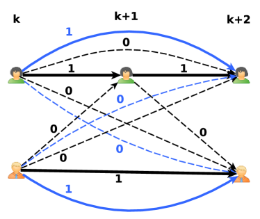 Figure 5: Illustration of a lifted disjoint paths problem on flow network (black edges) and lifted graph (blue edges).
Active edges are solid while inactive edges are dashed.
Figure 5: Illustration of a lifted disjoint paths problem on flow network (black edges) and lifted graph (blue edges).
Active edges are solid while inactive edges are dashed.
6.1 File Format
File defining costs between pairs of nodes.
Some of the pairs are selected to create flow edges, some of them are selected to create lifted edges according to the strategy for graph creation given by solver parameters. Note that lifted and flow edges can overlap. ⬇ ,, . . . ,,File defining the distribution of nodes in time frames.
Time frames are numbered from to (maximal time frame). Nodes are numbered from to . denotes nodes in time frame . ⬇ . . . . . . . . .File with solver parameters.
The file starts with the keyword [SOLVER] (including the brackets). Each parameter name is written with capital letters and underscores. Parameter values follow the sign. ⬇ [SOLVER] FIRST_PARAMETER_NAME=value1 SECOND_PARAMETER_NAME=value2 . . .Input file for the approximate solver.
We typically use the same set of parameters for processing all instances within a dataset. The first LDP solver LifT specifies path to instance files in the parameter file. Therefore, a separate parameter file is needed for each problem instance. Solver ApLift enables to use one parameter file for multiple instances. The path to instance files and to the parameter file is specified in the input input file that has the following format. ⬇ INPUT_GRAPH=/path/to/edge/costs INPUT_FRAMES=/path/to/nodes/in/frames INPUT_PARAMS=/path/to/parameter/file6.2 Datasets
6.2.1 MOT Challenge
The main application of LDP is in multiple object tracking. The MOT15/16/17 benchmarks [LTMR+15, MLTR+16] contain semi-crowded videos sequences filmed from a static or a moving camera. MOT20 [DRM+20] comprises crowded scenes with considerably higher number of frames and detections per frame.6.3 Algorithms
ILP Solver [HHRS20]: Cutting planes for ILP solvers together with a two-stage procedure for computing tracklets first. Message Passing Solver [HKS+21]: Decompose the full problem into combinatorially solved subproblems and link them together with Lagrange multipliers updated by block coordinate ascent.7 Graph Matching
The graph matching problem is equivalent to Lawler’s form of the quadratic assignment problem (QAP) from the combinatorial optimization literature. Given two point sets the task is to establish partial one-to-one correspondences between points in the respective sets.Definition 10 (Graph Matching).
Given and linear costs for and quadratic costs the graph matching problem is (11)7.1 File Format
We use the file format introduced by [TKR12]. ⬇ p A E a 1 . . . a A e . . . e where is the number of linear assignment terms (those that are not listed are assumed to have value ) and is the number of pairwise terms (those that are not listed are assumed to have value ). Linear assignments start with the identifier and are numbered from to . They go from node to with cost for . Quadratic costs start with the identifier and have cost , . The quadratic cost is incurred if both the -th and -th assignments are active. We also provide LP files for all instances.7.2 Benchmark datasets
7.2.1 Hotel & House212121https://keeper.mpdl.mpg.de/f/0fe3f173da55491cb10a/?dl=1
Matching of keypoints in two rigid objects [TKR12]. Images of the same object are taken at different angles and correspondences are computed from costs derived by appearance and geometric terms. There are 105 instances for each object with and dense linear and quadratic assignments.7.2.2 Worms222222https://keeper.mpdl.mpg.de/f/1058b4e0d8664c0bb0d5/?dl=1
Matching nuclei of C. elegans for automatic annotation [KJRM14] in bio-imaging. The 30 instances have up to points. Costs are sparse.7.3 Algorithms
Semidefinite Programming [SS05]: Semidefinite relaxation for graph matching. Dual Decomposition [TKR12]: Subgradient ascent on a dual decomposition of graph matching into max-flow, linear assignment and enumerative local subproblems. Hungarian BP [ZSM+16]: Message passing using additionally a linear assignment solver. Message Passing [SRAA+17] Several improved message passing schemes on different decompositions. Fusion Moves [HHF+21]: Explore subspaces of graph matchings generated randomly and solve with ILP solvers. Covering Trees [YFI10]: Convert the graph matching problem to one large tree MRF with additional Lagrange multipliers and optimize with message passing. DS* [BTM18]: A lifting-free convex relaxation approach. Semidefinite Optimization [KKBL15]: Semidefinite optimization problem formulation of multi-graph matching. Graduated assignment [GR96]: An algorithm combining graduated nonconvexity, two-way assignment constraints and sparsity. Tabu search [ASML15]: Reformulation of graph matching into an equivalent weighted maximum clique problem solved by tabu search. Fixed-point iteration [LHS09]: Climbing and convergence guaranteeing discretization scheme. Max-Pooling [CSDP14]: Matching through evaluating neighborhood candidates and gradually propagating matching scores to neighbors via max-pooling, eventually producing reliability matching scores. Spectral correspospondence finding [LH05]: Correct assignment clustering via principal eigenvector and additionally imposing mapping constraints. Umeyama’s Eigen-decomposition method [ZLTM07]: Generalization of Umeyama’s formula for graph matching and corresponding matching algorithm. Reweighted random walks [CLL10]: Graph matching formulation as node selection on an association graph solved by simulating random walks with reweighting jumps enforcing matching constraints. MCMC [LCL10]: Data-driven Markov Chain Monte Carlo sampling additionally using spectral properties of the graphs. Sequential Monte Carlo [SCL12]: Sequential Monte Carlo sampling a sequence of of intermediate target distributions with importance resampling for maximizing the graph matching objective. Path following [ZBV08]: A convex-concave programming formulation obtained by rewriting graph matching as a least-squares problem on the set of permutation matrices and solving a quadratic convex and concave problem. Factorized graph matching [ZDlT15]: Graph matching via affinity matrix factorization as a Kronecker product of smaller matrices solved approximately through a path-following Frank-Wolfe algorithm.8 Multi-Graph Matching
The multi-graph matching problem is an extension of the graph matching problem from Section 7 to more than two graphs with additional cycle consistency constraints ensuring that compositions of matchings are consistent.Definition 11 (Multi-Graph Matching).
Given and linear costs and quadratic costs for every , the multi-graph matching problem is (12) where we use for matrix multiplication and holds elementwise. An illustration of the multi-graph matching problem with matchings that obey resp. violate cycle consistency is given in Figure 7.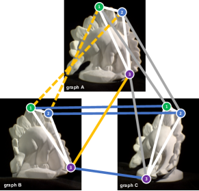 Figure 7:
Illustration of cycle consistency in multi-graph matching (best viewed in color).
Each graph , , comprises three nodes (green, blue, purple) and three edges (white lines).
The true correspondence is indicated by the node colour and node labels 1, 2, 3.
Matchings between pairs of graphs are shown by coloured lines ( in yellow, in gray, and in blue).
Wrong matchings are indicated by dashed lines.
The multi-matching is not cycle consistent.
Figure 7:
Illustration of cycle consistency in multi-graph matching (best viewed in color).
Each graph , , comprises three nodes (green, blue, purple) and three edges (white lines).
The true correspondence is indicated by the node colour and node labels 1, 2, 3.
Matchings between pairs of graphs are shown by coloured lines ( in yellow, in gray, and in blue).
Wrong matchings are indicated by dashed lines.
The multi-matching is not cycle consistent.
8.1 File Format
The file format is derived from the one for graph matching described in Section 7.1. ⬇ gm ### graph matching problem for ### ### matching with ### ### as in Section 7.1 ### . . . gm ### graph matching problem for ### ### matching with ### ### as in Section 7.1 ###8.2 Datasets
8.2.1 Hotel & House232323https://keeper.mpdl.mpg.de/f/d7ba7019eede485fb457/?dl=1
In this experiment we consider the CMU house and hotel sequences. of the points are outliers and the total number of points per image is . For problem generation we have followed the protocol of [41], where further details are described. Costs are computed as in [YCZ+15]. In total there are 80 instances, 40 for house and 40 for hotel.8.2.2 Synthetic242424https://keeper.mpdl.mpg.de/f/8ca51384836d40a09487/?dl=1
Four different categories (complete, density, deform, outlier) of synthetic multi-graph matching problems with the number of point sets varying from 4 to 16 generated as in [YCZ+15]. In total there are 160 instances, 40 from each category.8.2.3 Worms252525https://keeper.mpdl.mpg.de/f/8b1385731fae4febb4fe/?dl=1
Multi-graph matching instances generated from 30 images of C. elegans [KJRM14]. Points correspond to nuclei of the organism, which can number up to 558 per point set. Instances have from 3 to 10 randomly selected point sets. In total there are 400 instances, 50 per number of point sets.8.3 Algorithms
Permutation Synchronization [BTGT19, PKS13]: Non-negative matrix factorisation followed by Euclidean projection for binarization. Alternating Graph matching [YTZ+13, ZZD15, YWZ+15]: Alternating optimization between graph matching solvers and a cycle consistency-enforcing component. Graduated Consistency [YLL+14, YCZ+15]: Iterative approximation of the graph matching objective with gradual consistency enforcement. Matrix Decomposition [YXZ+15]: Matrix decomposition based formulation solved through convex optimization. Factorized Matching [ZDlT15]: Global alternating minimization approach via low-rank matrix recovery. Semidefinite Optimization [KKBL15]: Semidefinite optimization problem formulation of multi-graph matching. Fast Clustering [TZED17]: Clustering-based formulation identifying multi-image matchings from a density function in feature space. Tensor Power Iteration [SLH+16]: Rank-1 tensor approximation solved via power iteration. Mining Consistent Features [WZD18]: Multi-graph matching by matching sparse feature sets and geometric consistency through low-rank constraints. DS* [BTM18]: A lifting-free convex relaxation approach. Random Walk [PY19]: A multi-layer random walk synchronization approach. Convex Message Passing [SMT+19]: Lagrange decomposition optimized with message passing. Cycle consistency is enforced via a cutting plane procedure that adds tightening subproblems. HiPPi [BTST19]: A higher-order projected power iteration method.9 Cell Tracking
The cell tracking problem is to construct a lineage tree of cells across a time sequence with potentially dividing cells, see Figure 8 for an illustration. We use a general formulation incorporating mutually exclusive cell candidates originally proposed in [FAH+12].Definition 12 (Cell Tracking).
Let time steps, detection candidates for each time step, transition edges and division edges for and exclusion sets for be given. Define variables (13) The cell tracking problem is (14) such that (15) (16) (17) The first two constraints in (15) and (16) are flow conservation constraints stating that whenever a detection is active it must be linked to one detection in the previous timeframe and one or two in the next timeframe. The third constraint (17) stipulates that for each exclusion set at most one detection might be active (e.g. when multiple cell candidates overlap spatially).9.1 File Format
We use the file format also used in [HPH+20]. ⬇ # comment line # Cell detection hypotheses H . . . # Cell appearances, disappearances, # movement and divisions APP DISAPP MOVE DIV . . . # Exclusion constraints CONFSET + … + <= 1 . . . Comments start with #. Cell detections start with ‘H’, next comes the timeframe , then the id and last the detection cost . The ids must be unique also across timeframes. Cell appearance/disappearance start with ‘APP’ (resp. ‘DISAPP’), next comes the timeframe , then the id and last the appearance/disappearance cost . Cell movements start with ‘MOVE’, next come the movement id, then the ids of the two involved cell detections. Cell divisions start with ‘DIV’, next come the division id, then the ids of the three involved cell detections. Exclusion constraints start with ‘CONFSET’ and use the ids of the involved cell detections. We provide LP files for all cell tracking instances as well.9.2 Datasets
9.2.1 AISTATS 2020 dataset262626https://keeper.mpdl.mpg.de/f/da232900c06c46399fd0/?dl=1
We have taken an extended set of instances used in [HPH+20]. The instances can be grouped as follows.Drosophila embryo
One problem instance for tracking nuclei in a developing Drosophila embryo. The tracking models consists of up to 252 frames detection hypotheses each and true cells.Flywing
Tracking membrane-labelled cells in developing Drosophila flywing tissue. Instances have up to 245 frames with detection hypotheses per frame.Cell Tracking Challenge (CTC)
Publicly available cell tracking instances of sequences from [UMM+17]. Instances have up to 426 frames and up to 1400 detection hypotheses.9.3 Algorithms
Primal Dual Solver [HPH+20]: Use dual block coordinate ascent on a Lagrange decomposition and round primal solutions with a series of independent set problems. Generalized Network Flow [HAWH16]: Generalize the successive shortest path minimum cost flow algorithm to efficiently support cell divisions in a network flow model.10 Shape Matching
The shape matching problem is to find a mapping between shapes. For an illustration see Figure 9. We follow the shape matching formulation of [WSSC11a, WSSC11b]. Here the shape matching problem is posed as an ILP which ensures an orientation preserving geometrically consistent matching.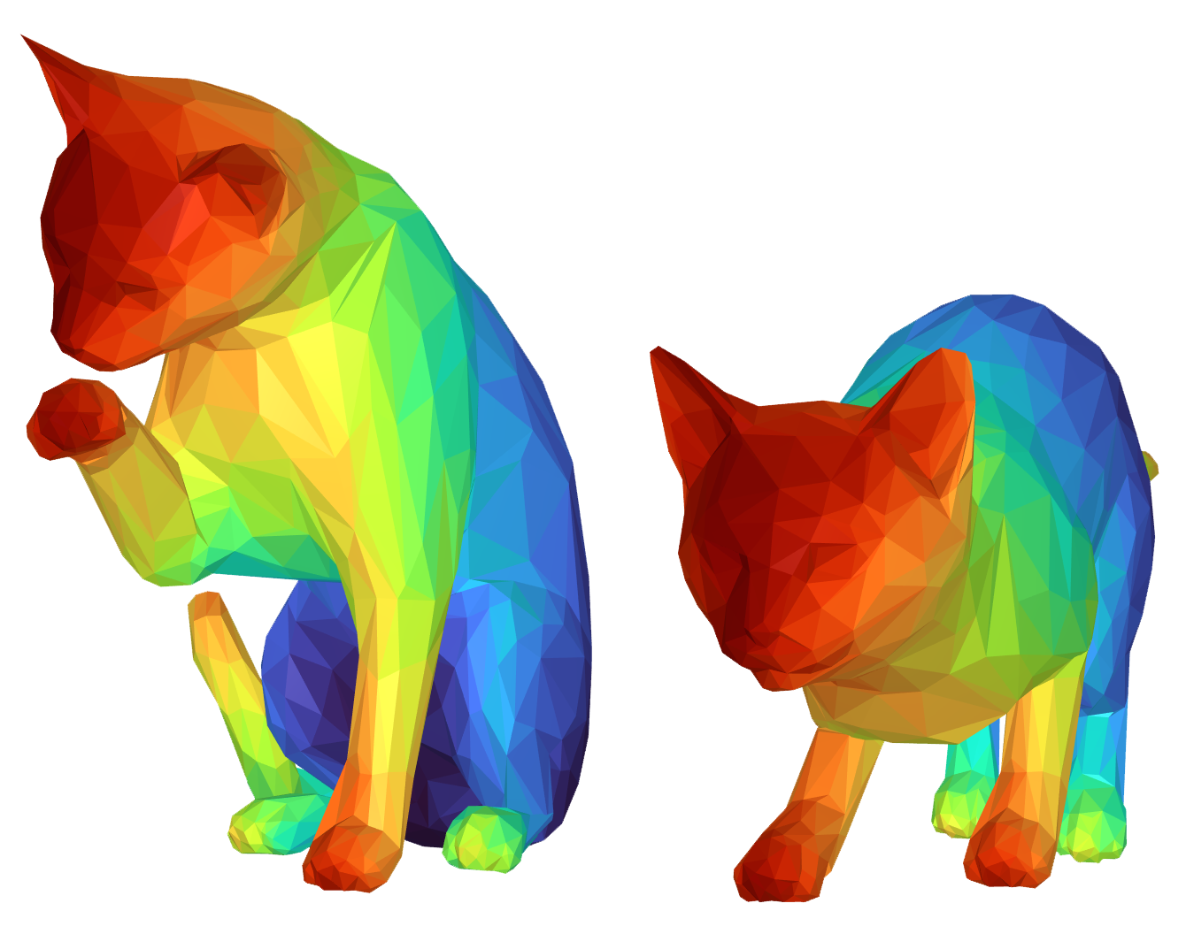 Figure 9: Shape matching of a cat in different poses. Colors encode matches of triangles.
Definition 13 (Shape).
We define a shape as a triplet of vertices , edges and triangles , such that the manifold induced by the triangles is oriented and has no boundaries.Definition 14 (Degenerate Triangles and Edges).
By we denote the set of degenerate triangles, that in addition to the triangles also contains triangles formed by edges (a triangle with two vertices at the same position) and triangles formed by vertices (a triangle with three vertices at the same position). Similarly, we consider the set of degenerate edges .Definition 15 (Product Spaces).
Let two shapes and be given. The triangle product space is defined as The edge product space is defined asDefinition 16 (Discrete Surfaces).
Let the triangle product space and the edge product space be given for a pair of shapes . A discrete surface is given by its indicator representation (18) The -th entry belongs to the -th triangle product in . Triangle products encode a matching between a triangle from and a triangle from . Hence, discrete surfaces encode a matching between and . Constraints are needed to ensure surjectivity and geometric consistency of the matching.Definition 17 (Projection Operator).
The projection is defined by (19) for all non-degenerate triangles . The projection operator is defined analoguously.Definition 18 (Surjectivity Constraint).
A given discrete surface ensures a surjective matching of with if it projects to each shape and such that (20) with and .Definition 19 (Orientation).
For the sets and an arbitrary orientation shall be defined. This implies an orientation for each edge product . By means of these orientations a vector can be defined for every edge product . The entries of write as (21)Definition 20 (Boundary Operator).
The boundary operator is defined for every triangle product by (22) where and form triangles in resp. and is the edge product connecting the product vertices and .Definition 21 (Closeness/Geometric Consistency Constraint).
A given discrete surface ensures a geometric consistent matching of with , i.e. is a closed discrete surface if it satisfies (23)Definition 22 (Discrete Graph Surfaces).
A graph surface is a discrete surface which fulfills the geometric consistency constraint as well as the surjectivity constraints.Definition 23 (Deformation Energy).
The deformation energy is defined for every triangle product. It describes the energy needed to deform the respective triangle from shape into the triangle from shape and vice versa. We now have all operators to define the shape matching problem as the search for a discrete graph surface.Definition 24 (Shape Matching).
Given an energy the shape matching problem is (24)10.1 File Format
Instances are given in the ILP file format from Section 1.2. The filenames contain information about the respective problems <# binvars>_<# constraints>_<shape X>_ (25) <# triangles>_<shape Y>_<# triangles>.lp Each binary variable belongs to a triangle product. Considering a vertices of shape as and a vertices of shape as respectively. The names of the binary variables are structured as follows (26) From the names the respective vertices or rather the respective triangle products can be identified.10.2 Datasets
10.2.1 TOSCA 272727https://keeper.mpdl.mpg.de/f/cf736ce0e16d4323a13b/?dl=1
A sample generated matching problems (LP-files) on TOSCA [BBK08] shapes. The dataset contains ILP files consisting of problems with binary variables up to binary variables. The dataset contains matching problems between complete shapes and partial shapes and shapes with equal triangulation. Partial shapes are shapes which are missing parts of the original shape (such files are denoted with _partial). Additionally, there are matching problems which are between non-isometric deformed shapes e.g. a cat matched with a dog (such files are denoted with _noniso).The original shapes are not included.
10.2.2 Deep Learning Predictor Energies 282828https://keeper.mpdl.mpg.de/f/3988e4dd09ce48438a79/?dl=1
A subset of shape matching problems (LP-files) containing in total ILP files consisting of problems with up to triangles in increments of . This translates to up to binary variables. Shape pairs for matching are taken from FAUST_r [RPWO18, DSO20], SMAL [ZKJB17], SHREC’20 [DLR+20] and DT4D-H [MRSHO22]. The energies are computed as in [RAC+23] using the shape descriptors from [CRB23].10.3 Algorithms
LP + incremental fixation [WSSC11a]: LP relaxation of (24) is solved with CPLEX [Cpl19] and franctional variables are incrementally fixed towards -values they are close to. Eckstein-Bertsekas [WSSC11b]: A GPU implementation of the parallelizable primal-dual algorithm proposed by Eckstein and Bertsekas [EB+90]. SMcomb [RSCB22]: Shape matchings are constructed by iterative fixing + propagation and backtracking algorithm using dual information computed by [LS21] as variable guidance. FastDOG-LBFGS + Constraint Splitting [RAC+23]: LP relaxation is solved with an extension of the GPU solver [AS22] that incorporates LBFGS for faster convergence and splitting long constraints into shorter ones for faster iterations. Rounding is performed with incremental perturbation until the dual produces a consistent primal solution as in [AS22].11 Discrete Tomography
The discrete tomography problem is the reconstruction of integral values given by a set of tomographic projections. It specializes the conventional tomographic reconstruction problem that allows for fractional values.Definition 25 (Discrete Tomography).
Given an MRF such that the label space is and a number of projections the discrete tomography problem is (27) Typically we have , that is the unary potentials do not give any preference. An illustration of tomographic projections is given in Figure 10.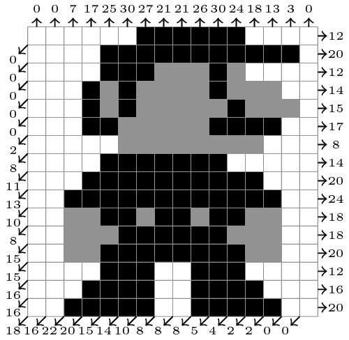 Figure 10:
Exemplary discrete tomography problem.
White pixels indicate value , gray ones and the black ones .
Each tomographic projection is indicated by an arrow and contains those pixels along its ray. The numbers correspond to .
Figure 10:
Exemplary discrete tomography problem.
White pixels indicate value , gray ones and the black ones .
Each tomographic projection is indicated by an arrow and contains those pixels along its ray. The numbers correspond to .
11.1 File Format
We use an extension of the UAI file format used for MRFs in Section 2.1. In addition to specifying the MRF structure the tomographic projections are appended. ⬇ UAI file format for MRF PROJECTIONS . . . + … = (Inf,…,Inf,,Inf,…,Inf) . . . for and .11.2 Datasets
11.2.1 Synthetic Discrete Tomography292929https://keeper.mpdl.mpg.de/f/8827141df8254eefbac4/?dl=1
Around discrete tomography instances computed from synthetically generated images with 3 discrete intensity values and varying density of observed objects measured by varying numbers of tomographic projections. Additionally larger discrete tomography instances of the “Logan” image are given.11.3 Algorithms
Subgradient ascent on submodular MRF & Projection [KPSZ15]: A binary discrete tomography solver using a Lagrange decomposition into submodular binary MRF solved with graph cuts and tomographic projection constraint solved via linear algebra. First-order optimization [ZKS+16]: Combination of total variation regularized reconstruction problem with a non-convex discrete constraint optimized with forward-backward splitting. Fixed-point iteration [ZPSS16]: Combination of a non-local projection constraint problem with a continuous convex relaxaton of the multilabeling problem solved by a fixed point iteration each of which amounts to solution of a convex auxiliary problem. Subgradient on decomposition into chain subproblems [KSP17]: Decompose original problems into chain subproblems that are recursively solved with fast (max,sum)-algorithms. The resulting Lagrange decomposition is optimized with a bundle solver. FW-Bundle Method [SK19]: Similar to [KSP17] but use a Frank-Wolfe based bundle method for optimization of the Lagrange decomposition.12 Bottleneck Markov Random Fields
The bottleneck Markov Random Field problem is an extension of the ordinary Markov Random Field inference problem from Section 2. The ordinary MRF problem is an optimization w.r.t. the -semiring (i.e. we minimize over a sum of potentials), while the inference over bottleneck MRFs is additional an optimization w.r.t. the -semiring (i.e. we also optimize over the maximum assignment of all potentials).Definition 26 (Bottleneck MRF).
Given an MRF (see Defintion 1) and additional bottleneck potentials for and for , the bottleneck MRF inference problem is (28)12.1 File Format
The file format is an extension of the uai file format proposed for MRFs in Section 2.1. ⬇ MARKOV MAX-POTENTIALS What follows after MARKOV is the ordinary MRF part describing potentials in Definition 26 and what follows after MAX-POTENTIALS are the potentials for the bottleneck part in Definition 26.12.2 Datasets
12.2.1 Horizon Tracking303030https://keeper.mpdl.mpg.de/f/4b0af028e879482b8037/?dl=1
12 horizon tracking instances and ground truth data for tracking subsurface rock layers generated from subsurface volumes F3 Netherlands, Opunake-3D, Waka-3D from The Society of Exploration Geophysicists.12.3 Algorithms
Lagrange Decomposition & Subgradient Ascent [AS19]: Combinatorial subproblems for ordinary tree MRFs and bottleneck chain MRFs joined via Lagrange multipliers and optimized via subgradient ascent.References
- [Ach09] Tobias Achterberg. Scip: solving constraint integer programs. Mathematical Programming Computation, 1(1):1–41, 2009.
- [AKB+11] Bjoern Andres, Jörg H. Kappes, Thorsten Beier, Ullrich Köthe, and Fred A. Hamprecht. Probabilistic image segmentation with closedness constraints. In ICCV, 2011.
- [AKB+12a] Bjoern Andres, Jörg H Kappes, Thorsten Beier, Ullrich Köthe, and Fred A Hamprecht. The lazy flipper: Efficient depth-limited exhaustive search in discrete graphical models. In European Conference on Computer Vision, pages 154–166. Springer, 2012.
- [AKB+12b] Bjoern Andres, Thorben Kröger, Kevin L. Briggman, Winfried Denk, Natalya Korogod, Graham Knott, Ullrich Köthe, and Fred A. Hamprecht. Globally optimal closed-surface segmentation for connectomics. In ECCV, 2012.
- [AKT09] Karteek Alahari, Pushmeet Kohli, and Philip HS Torr. Dynamic hybrid algorithms for map inference in discrete mrfs. IEEE Transactions on Pattern Analysis and Machine Intelligence, 32(10):1846–1857, 2009.
- [ApS19] MOSEK ApS. The MOSEK optimization toolbox for MATLAB manual. Version 9.0., 2019.
- [AS19] Ahmed Abbas and Paul Swoboda. Bottleneck potentials in markov random fields. In Proceedings of the IEEE/CVF International Conference on Computer Vision, pages 3175–3184, 2019.
- [AS21] Ahmed Abbas and Paul Swoboda. Combinatorial optimization for panoptic segmentation: A fully differentiable approach. Advances in Neural Information Processing Systems, 34:15635–15649, 2021.
- [AS22] Ahmed Abbas and Paul Swoboda. Fastdog: Fast discrete optimization on gpu. In Proceedings of the IEEE/CVF Conference on Computer Vision and Pattern Recognition, pages 439–449, 2022.
- [AS23] Ahmed Abbas and Paul Swoboda. Clusterfug: Clustering fully connected graphs by multicut. In International Conference on Machine Learning, ICML 2023, 23-29 July 2023, Honolulu, Hawaii, USA, volume 202 of Proceedings of Machine Learning Research, 2023.
- [ASML15] Kamil Adamczewski, Yumin Suh, and Kyoung Mu Lee. Discrete tabu search for graph matching. In Proceedings of the IEEE international conference on computer vision, pages 109–117, 2015.
- [BBK08] Alexander Bronstein, Michael Bronstein, and Ron Kimmel. Numerical Geometry of Non-Rigid Shapes. Springer Science & Business Media, 2008.
- [BDG+08] Ulrik Brandes, Daniel Delling, Marco Gaertler, Robert Gorke, Martin Hoefer, Zoran Nikoloski, and Dorothea Wagner. On modularity clustering. IEEE Transactions on Knowledge and Data Engineering, 20(2):172–188, 2008.
- [Bes86] Julian Besag. On the statistical analysis of dirty pictures. Journal of the Royal Statistical Society: Series B (Methodological), 48(3):259–279, 1986.
- [BK04] Yuri Boykov and Vladimir Kolmogorov. An experimental comparison of min-cut/max-flow algorithms for energy minimization in vision. IEEE transactions on pattern analysis and machine intelligence, 26(9):1124–1137, 2004.
- [BKK+14] Thorsten Beier, Thorben Kroeger, Jorg H Kappes, Ullrich Kothe, and Fred A Hamprecht. Cut, glue & cut: A fast, approximate solver for multicut partitioning. In Proceedings of the IEEE Conference on Computer Vision and Pattern Recognition, pages 73–80, 2014.
- [BPR+17] Thorsten Beier, Constantin Pape, Nasim Rahaman, Timo Prange, Stuart Berg, Davi D Bock, Albert Cardona, Graham W Knott, Stephen M Plaza, Louis K Scheffer, et al. Multicut brings automated neurite segmentation closer to human performance. Nature methods, 14(2):101, 2017.
- [BTGT19] Florian Bernard, Johan Thunberg, Jorge Goncalves, and Christian Theobalt. Synchronisation of partial multi-matchings via non-negative factorisations. Pattern Recognition, 92:146–155, 2019.
- [BTM18] Florian Bernard, Christian Theobalt, and Michael Moeller. Ds*: Tighter lifting-free convex relaxations for quadratic matching problems. In Proceedings of the IEEE conference on computer vision and pattern recognition, pages 4310–4319, 2018.
- [BTST19] Florian Bernard, Johan Thunberg, Paul Swoboda, and Christian Theobalt. Hippi: Higher-order projected power iterations for scalable multi-matching. In Proceedings of the IEEE/CVF International Conference on Computer Vision, pages 10284–10293, 2019.
- [BVZ01] Yuri Boykov, Olga Veksler, and Ramin Zabih. Fast approximate energy minimization via graph cuts. IEEE Transactions on pattern analysis and machine intelligence, 23(11):1222–1239, 2001.
- [CHL11] Sonia Cafieri, Pierre Hansen, and Leo Liberti. Locally optimal heuristic for modularity maximization of networks. Phys. Rev. E, 83:056105, May 2011.
- [CLL10] Minsu Cho, Jungmin Lee, and Kyoung Mu Lee. Reweighted random walks for graph matching. In European conference on Computer vision, pages 492–505. Springer, 2010.
- [COR+16] Marius Cordts, Mohamed Omran, Sebastian Ramos, Timo Rehfeld, Markus Enzweiler, Rodrigo Benenson, Uwe Franke, Stefan Roth, and Bernt Schiele. The cityscapes dataset for semantic urban scene understanding. In Proceedings of the IEEE conference on computer vision and pattern recognition, pages 3213–3223, 2016.
- [Cpl19] Cplex, IBM ILOG. CPLEX optimization studio 12.10, 2019.
- [CR93] Sunil Chopra and Mendu R Rao. The partition problem. Mathematical Programming, 59(1-3):87–115, 1993.
- [CRB23] Dongliang Cao, Paul Roetzer, and Florian Bernard. Unsupervised learning of robust spectral shape matching. ACM Transactions on Graphics (TOG), 2023.
- [cre] Cremi miccai challenge on circuit reconstruction from electron microscopy images. https://cremi.org.
- [CSDP14] Minsu Cho, Jian Sun, Olivier Duchenne, and Jean Ponce. Finding matches in a haystack: A max-pooling strategy for graph matching in the presence of outliers. In Proceedings of the IEEE Conference on Computer Vision and Pattern Recognition, pages 2083–2090, 2014.
- [DDMHL92] Johan Desmet, Marc De Maeyer, Bart Hazes, and Ignace Lasters. The dead-end elimination theorem and its use in protein side-chain positioning. Nature, 356(6369):539–542, 1992.
- [DDS+09] Jia Deng, Wei Dong, Richard Socher, Li-Jia Li, Kai Li, and Li Fei-Fei. Imagenet: A large-scale hierarchical image database. In 2009 IEEE conference on computer vision and pattern recognition, pages 248–255. Ieee, 2009.
- [DEFI06] Erik D Demaine, Dotan Emanuel, Amos Fiat, and Nicole Immorlica. Correlation clustering in general weighted graphs. Theoretical Computer Science, 361(2-3):172–187, 2006.
- [DLR+20] Roberto M. Dyke, Yu-Kun Lai, Paul L. Rosin, Stefano Zappalà, Seana Dykes, Daoliang Guo, Kun Li, Riccardo Marin, Simone Melzi, and Jingyu Yang. SHREC’20: Shape correspondence with non-isometric deformations. Computers & Graphics, 92:28–43, 2020.
- [DRM+20] Patrick Dendorfer, Hamid Rezatofighi, Anton Milan, Javen Shi, Daniel Cremers, Ian Reid, Stephan Roth, Konrad Schindler, and Laura Leal-Taixé. Mot20: A benchmark for multi object tracking in crowded scenes. arXiv:2003.09003[cs], March 2020. arXiv: 2003.09003.
- [DSO20] Nicolas Donati, Abhishek Sharma, and Maks Ovsjanikov. Deep geometric functional maps: Robust feature learning for shape correspondence. In Proceedings of the IEEE/CVF Conference on Computer Vision and Pattern Recognition, pages 8592–8601, 2020.
- [EB+90] Jonathan Eckstein, Dimitri P Bertsekas, et al. An alternating direction method for linear programming. Technical report, 1990.
- [EG11] G Elidan and A Globerson. The probabilistic inference challenge (pic2011), 2011.
- [FAH+12] Jan Funke, Bjoern Andres, Fred A Hamprecht, Albert Cardona, and Matthew Cook. Efficient automatic 3d-reconstruction of branching neurons from em data. In 2012 IEEE Conference on Computer Vision and Pattern Recognition, pages 1004–1011. IEEE, 2012.
- [GBV+14] Lena Gorelick, Yuri Boykov, Olga Veksler, Ismail Ben Ayed, and Andrew Delong. Submodularization for binary pairwise energies. In Proceedings of the IEEE Conference on Computer Vision and Pattern Recognition, pages 1154–1161, 2014.
- [GJ07] Amir Globerson and Tommi Jaakkola. Fixing max-product: Convergent message passing algorithms for map lp-relaxations. Advances in neural information processing systems, 20:553–560, 2007.
- [GO19] LLC Gurobi Optimization. Gurobi optimizer reference manual, 2019.
- [GR96] Steven Gold and Anand Rangarajan. A graduated assignment algorithm for graph matching. IEEE Transactions on pattern analysis and machine intelligence, 18(4):377–388, 1996.
- [HAWH16] Carsten Haubold, Janez Aleš, Steffen Wolf, and Fred A Hamprecht. A generalized successive shortest paths solver for tracking dividing targets. In European Conference on Computer Vision, pages 566–582. Springer, 2016.
- [HCKK21] Kalun Ho, Avraam Chatzimichailidis, Margret Keuper, and Janis Keuper. Msm: Multi-stage multicuts for scalable image clustering. In International Conference on High Performance Computing, pages 267–284. Springer, 2021.
- [HHF+21] Lisa Hutschenreiter, Stefan Haller, Lorenz Feineis, Carsten Rother, Dagmar Kainmüller, and Bogdan Savchynskyy. Fusion moves for graph matching. In Proceedings of the IEEE/CVF International Conference on Computer Vision, pages 6270–6279, 2021.
- [HHRS20] Andrea Hornakova, Roberto Henschel, Bodo Rosenhahn, and Paul Swoboda. Lifted disjoint paths with application in multiple object tracking. In International Conference on Machine Learning, pages 4364–4375. PMLR, 2020.
- [HKS+21] Andrea Hornakova, Timo Kaiser, Paul Swoboda, Michal Rolinek, Bodo Rosenhahn, and Roberto Henschel. Making higher order mot scalable: An efficient approximate solver for lifted disjoint paths. In Proceedings of the IEEE/CVF International Conference on Computer Vision, pages 6330–6340, 2021.
- [HPH+20] Stefan Haller, Mangal Prakash, Lisa Hutschenreiter, Tobias Pietzsch, Carsten Rother, Florian Jug, Paul Swoboda, and Bogdan Savchynskyy. A primal-dual solver for large-scale tracking-by-assignment. In International Conference on Artificial Intelligence and Statistics, pages 2539–2549. PMLR, 2020.
- [HSS18] Stefan Haller, Paul Swoboda, and Bogdan Savchynskyy. Exact map-inference by confining combinatorial search with lp relaxation. In Thirty-Second AAAI Conference on Artificial Intelligence, 2018.
- [JEMF06] Ariel Jaimovich, Gal Elidan, Hanah Margalit, and Nir Friedman. Towards an integrated protein–protein interaction network: A relational markov network approach. Journal of Computational Biology, 13(2):145–164, 2006.
- [KAH+15] Jörg H Kappes, Bjoern Andres, Fred A Hamprecht, Christoph Schnörr, Sebastian Nowozin, Dhruv Batra, Sungwoong Kim, Bernhard X Kausler, Thorben Kröger, Jan Lellmann, et al. A comparative study of modern inference techniques for structured discrete energy minimization problems. International Journal of Computer Vision, 115(2):155–184, 2015.
- [KJRM14] Dagmar Kainmueller, Florian Jug, Carsten Rother, and Gene Myers. Active graph matching for automatic joint segmentation and annotation of c. elegans. In International Conference on Medical Image Computing and Computer-Assisted Intervention, pages 81–88. Springer, 2014.
- [KK18] Amirhossein Kardoost and Margret Keuper. Solving minimum cost lifted multicut problems by node agglomeration. In Asian Conference on Computer Vision, pages 74–89. Springer, 2018.
- [KKB+14] Thorben Kroeger, Jörg H Kappes, Thorsten Beier, Ullrich Koethe, and Fred A Hamprecht. Asymmetric cuts: Joint image labeling and partitioning. In German Conference on Pattern Recognition, pages 199–211. Springer, 2014.
- [KKBL15] Itay Kezurer, Shahar Z Kovalsky, Ronen Basri, and Yaron Lipman. Tight relaxation of quadratic matching. In Computer Graphics Forum, volume 34, pages 115–128. Wiley Online Library, 2015.
- [KLB+15] Margret Keuper, Evgeny Levinkov, Nicolas Bonneel, Guillaume Lavoué, Thomas Brox, and Bjorn Andres. Efficient decomposition of image and mesh graphs by lifted multicuts. In Proceedings of the IEEE International Conference on Computer Vision, pages 1751–1759, 2015.
- [KMWL08] Graham Knott, Herschel Marchman, David Wall, and Ben Lich. Serial section scanning electron microscopy of adult brain tissue using focused ion beam milling. Journal of Neuroscience, 28(12):2959–2964, 2008.
- [Kol05] Vladimir Kolmogorov. Convergent tree-reweighted message passing for energy minimization. In International Workshop on Artificial Intelligence and Statistics, pages 182–189. PMLR, 2005.
- [Kol14] Vladimir Kolmogorov. A new look at reweighted message passing. IEEE transactions on pattern analysis and machine intelligence, 37(5):919–930, 2014.
- [KPSZ15] Jörg Hendrik Kappes, Stefania Petra, Christoph Schnörr, and Matthias Zisler. Tomogc: Binary tomography by constrained graphcuts. In German Conference on Pattern Recognition, pages 262–273. Springer, 2015.
- [KPT07] Nikos Komodakis, Nikos Paragios, and Georgios Tziritas. Mrf optimization via dual decomposition: Message-passing revisited. In 2007 IEEE 11th International Conference on Computer Vision, pages 1–8. IEEE, 2007.
- [KR07] Vladimir Kolmogorov and Carsten Rother. Minimizing nonsubmodular functions with graph cuts-a review. IEEE transactions on pattern analysis and machine intelligence, 29(7):1274–1279, 2007.
- [KSP17] Jan Kuske, Paul Swoboda, and Stefania Petra. A novel convex relaxation for non-binary discrete tomography. In International Conference on Scale Space and Variational Methods in Computer Vision, pages 235–246. Springer, 2017.
- [KSR+08] Pushmeet Kohli, Alexander Shekhovtsov, Carsten Rother, Vladimir Kolmogorov, and Philip Torr. On partial optimality in multi-label mrfs. In Proceedings of the 25th international conference on Machine learning, pages 480–487, 2008.
- [KSS12] Jörg Hendrik Kappes, Bogdan Savchynskyy, and Christoph Schnörr. A bundle approach to efficient map-inference by lagrangian relaxation. In 2012 IEEE Conference on Computer Vision and Pattern Recognition, pages 1688–1695. IEEE, 2012.
- [LAS19] Jan-Hendrik Lange, Bjoern Andres, and Paul Swoboda. Combinatorial persistency criteria for multicut and max-cut. In Proceedings of the IEEE/CVF Conference on Computer Vision and Pattern Recognition, pages 6093–6102, 2019.
- [LCL10] Jungmin Lee, Minsu Cho, and Kyoung Mu Lee. A graph matching algorithm using data-driven markov chain monte carlo sampling. In 2010 20th International Conference on Pattern Recognition, pages 2816–2819. IEEE, 2010.
- [LH05] Marius Leordeanu and Martial Hebert. A spectral technique for correspondence problems using pairwise constraints. 2005.
- [LHS09] Marius Leordeanu, Martial Hebert, and Rahul Sukthankar. An integer projected fixed point method for graph matching and map inference. In Advances in neural information processing systems, pages 1114–1122. Citeseer, 2009.
- [LKA17] Evgeny Levinkov, Alexander Kirillov, and Bjoern Andres. A comparative study of local search algorithms for correlation clustering. In German Conference on Pattern Recognition, pages 103–114. Springer, 2017.
- [LKA18] Jan-Hendrik Lange, Andreas Karrenbauer, and Bjoern Andres. Partial optimality and fast lower bounds for weighted correlation clustering. In International Conference on Machine Learning, pages 2898–2907, 2018.
- [LKSY20] Jovita Lukasik, Margret Keuper, Maneesh Singh, and Julian Yarkony. A benders decomposition approach to correlation clustering. In 2020 IEEE/ACM Workshop on Machine Learning in High Performance Computing Environments (MLHPC) and Workshop on Artificial Intelligence and Machine Learning for Scientific Applications (AI4S), pages 9–16. IEEE, 2020.
- [LMB+14] Tsung-Yi Lin, Michael Maire, Serge Belongie, James Hays, Pietro Perona, Deva Ramanan, Piotr Dollár, and C Lawrence Zitnick. Microsoft coco: Common objects in context. In European conference on computer vision, pages 740–755. Springer, 2014.
- [LS11] Jan Lellmann and Christoph Schnörr. Continuous multiclass labeling approaches and algorithms. SIAM Journal on Imaging Sciences, 4(4):1049–1096, 2011.
- [LS21] Jan-Hendrik Lange and Paul Swoboda. Efficient message passing for 0–1 ilps with binary decision diagrams. In International Conference on Machine Learning, pages 6000–6010. PMLR, 2021.
- [LTMR+15] L. Leal-Taixé, A. Milan, I. Reid, S. Roth, and K. Schindler. MOTChallenge 2015: Towards a benchmark for multi-target tracking. arXiv:1504.01942 [cs], April 2015. arXiv: 1504.01942.
- [MFTM01] D. Martin, C. Fowlkes, D. Tal, and J. Malik. A database of human segmented natural images and its application to evaluating segmentation algorithms and measuring ecological statistics. In Proc. 8th Int’l Conf. Computer Vision, volume 2, pages 416–423, July 2001.
- [MKB+17] Frank Michel, Alexander Kirillov, Eric Brachmann, Alexander Krull, Stefan Gumhold, Bogdan Savchynskyy, and Carsten Rother. Global hypothesis generation for 6d object pose estimation. In Proceedings of the IEEE Conference on Computer Vision and Pattern Recognition, pages 462–471, 2017.
- [MLTR+16] Anton Milan, Laura Leal-Taixé, Ian Reid, Stephan Roth, and Konrad Schindler. MOT16: A benchmark for multi-object tracking. arXiv:1603.00831 [cs], March 2016. arXiv: 1603.00831.
- [MRSHO22] Robin Magnet, Jing Ren, Olga Sorkine-Hornung, and Maks Ovsjanikov. Smooth non-rigid shape matching via effective dirichlet energy optimization. In International Conference on 3D Vision (3DV), 2022.
- [Pap21] Constantin Pape. torch-em. https://github.com/constantinpape/torch-em, 2021.
- [PBL+17] Constantin Pape, Thorsten Beier, Peter Li, Viren Jain, Davi D Bock, and Anna Kreshuk. Solving large multicut problems for connectomics via domain decomposition. In Proceedings of the IEEE International Conference on Computer Vision, pages 1–10, 2017.
- [PKS13] Deepti Pachauri, Risi Kondor, and Vikas Singh. Solving the multi-way matching problem by permutation synchronization. In Advances in neural information processing systems, pages 1860–1868. Citeseer, 2013.
- [PY19] Han-Mu Park and Kuk-Jin Yoon. Consistent multiple graph matching with multi-layer random walks synchronization. Pattern Recognition Letters, 127:76–84, 2019.
- [RAC+23] Paul Roetzer, Ahmed Abbas, Dongliang Cao, Florian Bernard, and Paul Swoboda. Fast discrete optimisation for geometrically consistent 3d shape matching. arXiv preprint arXiv:2310.08230, 2023.
- [RKLS07] Carsten Rother, Vladimir Kolmogorov, Victor Lempitsky, and Martin Szummer. Optimizing binary mrfs via extended roof duality. In 2007 IEEE conference on computer vision and pattern recognition, pages 1–8. IEEE, 2007.
- [RPWO18] Jing Ren, Adrien Poulenard, Peter Wonka, and Maks Ovsjanikov. Continuous and orientation-preserving correspondences via functional maps. ACM Transactions on Graphics (ToG), 37:1–16, 2018.
- [RSCB22] Paul Roetzer, Paul Swoboda, Daniel Cremers, and Florian Bernard. A scalable combinatorial solver for elastic geometrically consistent 3d shape matching. In Proceedings of the IEEE/CVF Conference on Computer Vision and Pattern Recognition, pages 428–438, 2022.
- [S+19] Bogdan Savchynskyy et al. Discrete graphical models—an optimization perspective. Foundations and Trends® in Computer Graphics and Vision, 11(3-4):160–429, 2019.
- [SA17] Paul Swoboda and Bjoern Andres. A message passing algorithm for the minimum cost multicut problem. In Proceedings of the IEEE Conference on Computer Vision and Pattern Recognition, pages 1617–1626, 2017.
- [SA23] David Stein and Bjoern Andres. Correlation clustering of bird sounds. arXiv preprint arXiv:2306.09906, 2023. Accepted at GCPR 2023. In print.
- [Sch10] Nic Schraudolph. Polynomial-time exact inference in np-hard binary mrfs via reweighted perfect matching. In Proceedings of the Thirteenth International Conference on Artificial Intelligence and Statistics, pages 717–724. JMLR Workshop and Conference Proceedings, 2010.
- [SCL12] Yumin Suh, Minsu Cho, and Kyoung Mu Lee. Graph matching via sequential monte carlo. In European Conference on Computer Vision, pages 624–637. Springer, 2012.
- [She14] Alexander Shekhovtsov. Maximum persistency in energy minimization. In Proceedings of the IEEE Conference on Computer Vision and Pattern Recognition, pages 1162–1169, 2014.
- [She16] Alexander Shekhovtsov. Higher order maximum persistency and comparison theorems. Computer vision and image understanding, 143:54–79, 2016.
- [SJ09] David Sontag and Tommi Jaakkola. Tree block coordinate descent for map in graphical models. In Artificial Intelligence and Statistics, pages 544–551. PMLR, 2009.
- [SK19] Paul Swoboda and Vladimir Kolmogorov. Map inference via block-coordinate frank-wolfe algorithm. In Proceedings of the IEEE/CVF Conference on Computer Vision and Pattern Recognition, pages 11146–11155, 2019.
- [SKSS11] Bogdan Savchynskyy, Jörg Kappes, Stefan Schmidt, and Christoph Schnörr. A study of nesterov’s scheme for lagrangian decomposition and map labeling. In CVPR 2011, pages 1817–1823. IEEE, 2011.
- [SKSS13] Bogdan Savchynskyy, Jörg Hendrik Kappes, Paul Swoboda, and Christoph Schnörr. Global map-optimality by shrinking the combinatorial search area with convex relaxation. Advances in Neural Information Processing Systems, 26:1950–1958, 2013.
- [SL+12] David Sontag, Yitao Li, et al. Efficiently searching for frustrated cycles in map inference. In 28th Conference on Uncertainty in Artificial Intelligence, UAI 2012, pages 795–804, 2012.
- [SLH+16] Xinchu Shi, Haibin Ling, Weiming Hu, Junliang Xing, and Yanning Zhang. Tensor power iteration for multi-graph matching. In Proceedings of the IEEE conference on computer vision and pattern recognition, pages 5062–5070, 2016.
- [SMT+19] Paul Swoboda, Ashkan Mokarian, Christian Theobalt, Florian Bernard, et al. A convex relaxation for multi-graph matching. In Proceedings of the IEEE/CVF Conference on Computer Vision and Pattern Recognition, pages 11156–11165, 2019.
- [SRAA+17] Paul Swoboda, Carsten Rother, Hassan Abu Alhaija, Dagmar Kainmuller, and Bogdan Savchynskyy. A study of lagrangean decompositions and dual ascent solvers for graph matching. In Proceedings of the IEEE conference on computer vision and pattern recognition, pages 1607–1616, 2017.
- [SRGP16] Alexander Shekhovtsov, Christian Reinbacher, Gottfried Graber, and Thomas Pock. Solving dense image matching in real-time using discrete-continuous optimization. In Proceedings of the 21st Computer Vision Winter Workshop (CVWW), page 13, 2016.
- [SS05] Christian Schellewald and Christoph Schnörr. Probabilistic subgraph matching based on convex relaxation. In International Workshop on Energy Minimization Methods in Computer Vision and Pattern Recognition, pages 171–186. Springer, 2005.
- [SSKS11] Stefan Schmidt, Bogdan Savchynskyy, Jörg Hendrik Kappes, and Christoph Schnörr. Evaluation of a first-order primal-dual algorithm for mrf energy minimization. In International Workshop on Energy Minimization Methods in Computer Vision and Pattern Recognition, pages 89–103. Springer, 2011.
- [SSKS12] Bogdan Savchynskyy, Stefan Schmidt, Jörg Kappes, and Christoph Schnörr. Efficient mrf energy minimization via adaptive diminishing smoothing. In Proceedings of the Twenty-Eighth Conference on Uncertainty in Artificial Intelligence, pages 746–755, 2012.
- [SSKS13] Paul Swoboda, Bogdan Savchynskyy, Jörg Kappes, and Christoph Schnörr. Partial optimality via iterative pruning for the potts model. In International Conference on Scale Space and Variational Methods in Computer Vision, pages 477–488. Springer, 2013.
- [SSKS14] Paul Swoboda, Bogdan Savchynskyy, Jorg H Kappes, and Christoph Schnorr. Partial optimality by pruning for map-inference with general graphical models. In Proceedings of the IEEE Conference on Computer Vision and Pattern Recognition, pages 1170–1177, 2014.
- [SSS15] Alexander Shekhovtsov, Paul Swoboda, and Bogdan Savchynskyy. Maximum persistency via iterative relaxed inference with graphical models. In Proceedings of the IEEE Conference on Computer Vision and Pattern Recognition, pages 521–529, 2015.
- [SZS+08] Richard Szeliski, Ramin Zabih, Daniel Scharstein, Olga Veksler, Vladimir Kolmogorov, Aseem Agarwala, Marshall Tappen, and Carsten Rother. A comparative study of energy minimization methods for markov random fields with smoothness-based priors. IEEE transactions on pattern analysis and machine intelligence, 30(6):1068–1080, 2008.
- [TKR12] Lorenzo Torresani, Vladimir Kolmogorov, and Carsten Rother. A dual decomposition approach to feature correspondence. IEEE transactions on pattern analysis and machine intelligence, 35(2):259–271, 2012.
- [TSRS18] Siddharth Tourani, Alexander Shekhovtsov, Carsten Rother, and Bogdan Savchynskyy. MPLP++: Fast, parallel dual block-coordinate ascent for dense graphical models. In Proceedings of the European Conference on Computer Vision (ECCV), pages 251–267, 2018.
- [TSRS20] Siddharth Tourani, Alexander Shekhovtsov, Carsten Rother, and Bogdan Savchynskyy. Taxonomy of dual block-coordinate ascent methods for discrete energy minimization. In International Conference on Artificial Intelligence and Statistics, pages 2775–2785. PMLR, 2020.
- [TZED17] Roberto Tron, Xiaowei Zhou, Carlos Esteves, and Kostas Daniilidis. Fast multi-image matching via density-based clustering. In Proceedings of the IEEE international conference on computer vision, pages 4057–4066, 2017.
- [UMM+17] Vladimír Ulman, Martin Maška, Klas EG Magnusson, Olaf Ronneberger, Carsten Haubold, Nathalie Harder, Pavel Matula, Petr Matula, David Svoboda, Miroslav Radojevic, et al. An objective comparison of cell-tracking algorithms. Nature methods, 14(12):1141–1152, 2017.
- [WD13] Huayan Wang and Koller Daphne. Subproblem-tree calibration: A unified approach to max-product message passing. In International Conference on Machine Learning, pages 190–198. PMLR, 2013.
- [Wer07] Tomas Werner. A linear programming approach to max-sum problem: A review. IEEE transactions on pattern analysis and machine intelligence, 29(7):1165–1179, 2007.
- [WSSC11a] Thomas Windheuser, Ulrich Schlickewei, Frank R Schmidt, and Daniel Cremers. Geometrically consistent elastic matching of 3d shapes: A linear programming solution. In 2011 International Conference on Computer Vision, pages 2134–2141. IEEE, 2011.
- [WSSC11b] Thomas Windheuser, Ulrich Schlickwei, Frank R Schimdt, and Daniel Cremers. Large-scale integer linear programming for orientation preserving 3d shape matching. In Computer Graphics Forum, volume 30, pages 1471–1480. Wiley Online Library, 2011.
- [WZD18] Qianqian Wang, Xiaowei Zhou, and Kostas Daniilidis. Multi-image semantic matching by mining consistent features. In Proceedings of the IEEE conference on computer vision and pattern recognition, pages 685–694, 2018.
- [YCZ+15] Junchi Yan, Minsu Cho, Hongyuan Zha, Xiaokang Yang, and Stephen M Chu. Multi-graph matching via affinity optimization with graduated consistency regularization. IEEE transactions on pattern analysis and machine intelligence, 38(6):1228–1242, 2015.
- [YFI10] Julian Yarkony, Charless Fowlkes, and Alexander Ihler. Covering trees and lower-bounds on quadratic assignment. In 2010 IEEE Computer Society Conference on Computer Vision and Pattern Recognition, pages 887–894. IEEE, 2010.
- [YIF11] Julian Yarkony, Alexander T Ihler, and Charless C Fowlkes. Planar cycle covering graphs. In Proceedings of the Twenty-Seventh Conference on Uncertainty in Artificial Intelligence, pages 761–769, 2011.
- [YLL+14] Junchi Yan, Yin Li, Wei Liu, Hongyuan Zha, Xiaokang Yang, and Stephen Mingyu Chu. Graduated consistency-regularized optimization for multi-graph matching. In European Conference on Computer Vision, pages 407–422. Springer, 2014.
- [YTZ+13] Junchi Yan, Yu Tian, Hongyuan Zha, Xiaokang Yang, Ya Zhang, and Stephen M Chu. Joint optimization for consistent multiple graph matching. In Proceedings of the IEEE international conference on computer vision, pages 1649–1656, 2013.
- [YWZ+15] Junchi Yan, Jun Wang, Hongyuan Zha, Xiaokang Yang, and Stephen Chu. Consistency-driven alternating optimization for multigraph matching: A unified approach. IEEE Transactions on Image Processing, 24(3):994–1009, 2015.
- [YXZ+15] Junchi Yan, Hongteng Xu, Hongyuan Zha, Xiaokang Yang, Huanxi Liu, and Stephen Chu. A matrix decomposition perspective to multiple graph matching. In Proceedings of the IEEE international conference on computer vision, pages 199–207, 2015.
- [ZBV08] Mikhail Zaslavskiy, Francis Bach, and Jean-Philippe Vert. A path following algorithm for the graph matching problem. IEEE Transactions on Pattern Analysis and Machine Intelligence, 31(12):2227–2242, 2008.
- [ZDlT15] Feng Zhou and Fernando De la Torre. Factorized graph matching. IEEE transactions on pattern analysis and machine intelligence, 38(9):1774–1789, 2015.
- [ZKJB17] Silvia Zuffi, Angjoo Kanazawa, David W Jacobs, and Michael J Black. 3d menagerie: Modeling the 3d shape and pose of animals. In CVPR, 2017.
- [ZKS+16] Matthias Zisler, Jörg Hendrik Kappes, Claudius Schnörr, Stefania Petra, and Christoph Schnörr. Non-binary discrete tomography by continuous non-convex optimization. IEEE Transactions on Computational Imaging, 2(3):335–347, 2016.
- [ZLP+18] Zhihao Zheng, J Scott Lauritzen, Eric Perlman, Camenzind G Robinson, Matthew Nichols, Daniel Milkie, Omar Torrens, John Price, Corey B Fisher, Nadiya Sharifi, et al. A complete electron microscopy volume of the brain of adult drosophila melanogaster. Cell, 174(3):730–743, 2018.
- [ZLTM07] Guoxing Zhao, Bin Luo, Jin Tang, and Jinxin Ma. Using eigen-decomposition method for weighted graph matching. In International Conference on Intelligent Computing, pages 1283–1294. Springer, 2007.
- [ZPSS16] Matthias Zisler, Stefania Petra, Claudius Schnörr, and Christoph Schnörr. Discrete tomography by continuous multilabeling subject to projection constraints. In German Conference on Pattern Recognition, pages 261–272. Springer, 2016.
- [ZSM+16] Zhen Zhang, Qinfeng Shi, Julian McAuley, Wei Wei, Yanning Zhang, and Anton Van Den Hengel. Pairwise matching through max-weight bipartite belief propagation. In Proceedings of the IEEE conference on computer vision and pattern recognition, pages 1202–1210, 2016.
- [ZZD15] Xiaowei Zhou, Menglong Zhu, and Kostas Daniilidis. Multi-image matching via fast alternating minimization. In Proceedings of the IEEE International Conference on Computer Vision, pages 4032–4040, 2015.