Likelihood-based Inference for Exponential-Family Random Graph Models via Linear Programming

Abstract

This article discusses the problem of determining whether a given point, or set of points, lies within the convex hull of another set of points in $d$ dimensions. This problem arises naturally in a statistical context when using a particular approximation to the loglikelihood function for an exponential family model; in particular, we discuss the application to network models here. While the convex hull question may be solved via a simple linear program, this approach is not well known in the statistical literature. Furthermore, this article details several substantial improvements to the convex hull-testing algorithm currently implemented in the widely used ergm package for network modeling.

Keywords convex hull  $\cdot$ duality  $\cdot$ MCMC  $\cdot$ missing data

1 Monte Carlo maximum likelihood estimation for exponential families

Suppose that we observe a complex data structure ${Y}$ from a sample space $\mathcal{Y}$, and we believe that the process that produced ${Y}$ may be captured sufficiently by the $d$-dimensional vector statistic $\bm{g}:\mathcal{Y}\mapsto\mathbb{R}^{d}$. A natural probability model for such an object—one that minimises the additional assumptions made in the sense of maximising entropy—is the exponential family class of models (Jaynes, 1957). If ${Y}$ modelled via a discrete or a continuous distribution, the probability mass function or density has the form, parametrized by the canonical parameter $\bm{\theta}\in\mathbb{R}^{d}$ (Barndorff-Nielsen, 1978, among others),

$$p_{\bm{\theta};\mathcal{Y},h,\bm{g}}({Y})=h({Y})\frac{\exp\{\bm{\theta}{{}^{\top}}\bm{g}({Y})\}}{\kappa_{\mathcal{Y},h,\bm{g}}(\bm{\theta})},\ {Y}\in\mathcal{Y}.$$

The form is then a product of a function $h(\cdot)$ of the data alone specifying the distribution under $\bm{\theta}=\bm{0}$, a function $\kappa(\cdot)$ of the parameter alone, defined below, and an exponential with the data’s and parameter’s interaction. The exact form of $\kappa(\bm{\theta})$ depends on the type of distribution:

discrete: $$\kappa_{\mathcal{Y},h,\bm{g}}(\bm{\theta}) =\sum_{{Y}^{\prime}\in\mathcal{Y}}h({Y})\exp\{\bm{\theta}{{}^{\top}}\bm{g}({Y}^{\prime})\}$$ (1a)

continuous: $$\kappa_{\mathcal{Y},h,\bm{g}}(\bm{\theta}) =\int_{\mathcal{Y}}h({Y})\exp\{\bm{\theta}{{}^{\top}}\bm{g}({Y}^{\prime})\}d{Y}^{\prime}.$$ (1b)

(A full measure-theoretic formulation is also possible for distributions that are neither discrete nor continuous; and a $\bm{\theta}\in\mathbb{R}^{q}$ for $q\leq d$ may be mapped through a vector function $\bm{\eta}:\mathbb{R}^{q}\mapsto\mathbb{R}^{d}$.) Likelihood-based inference for exponential-family models centers on the log-likelihood function

$$\ell(\bm{\theta})=\bm{\theta}{{}^{\top}}\bm{g}({Y}_{\text{obs}})-\log\kappa_{\mathcal{Y},h,\bm{g}}(\bm{\theta}).$$ (2)

Likelihood calculations can be highly computationally challenging when the sum or integral (1) is intractable (e.g., Geyer and Thompson, 1992).

For the sake of brevity, we will omit “$\mathcal{Y},h,\bm{g}$” from the subscript of $p_{\bm{\theta};\mathcal{Y},h,\bm{g}}({Y})$ and $\kappa_{\mathcal{Y},h,\bm{g}}(\bm{\theta})$ for the remainder of this paper, unless they differ from these defaults.

Most commonly, exponential families are used as a tool for deriving inferential properties of families that belong to this class, albeit with a different parametrization. For a common example, the canonical parameter of the $\operatorname{Normal}(\mu,\sigma^{2})$ distribution in its exponential family form is $\bm{\theta}=[\mu\sigma^{-2},\sigma^{-2}]$, which is far less convenient and interpretable.

However, there are domains in which an exponential family model is specified directly through its sufficient statistics, often with the help of the Hammersley–Clifford Theorem (Besag, 1974, among others). These include the Strauss spatial point processes (Strauss, 1975), the Conway–Maxwell–Poisson model for count data (Shmueli et al., 2005), and exponential-family random graph models (ERGMs) (Holland and Leinhardt, 1981; Frank and Strauss, 1986, for original derivations) for networks and other relational data. While our development is motivated by and focuses on ERGMs, it applies to other scenarios involving exponential-family models with intractable normalizing constants because the methods we discuss operate on the sufficient statistic $\bm{g}({Y})$ rather than on the original data structure.

Consider a graph ${Y}$ on $n$ vertices, with the vertices being labelled $1,\dotsc,n$. We will focus on binary undirected graphs with no self-loops and no further constraints—a discrete distribution. Thus, we can express $\mathcal{Y}=2^{\{\{i,j\}\in\{1,\dotsc,n\}^{2}:i\neq j\}}$, the power set of the set of all distinct unordered pairs of vertex indices.

An exponential family on such a sample space is called an exponential-family random graph model (ERGM). Substantively, elements of $\bm{g}({Y})$ then represent features of the graph—e.g., the number of edges or other structures, or connections between exogenously defined groups—whose prevalence is hypothesised to influence the relative likelihoods of different graphs.

For example, an edge count statistic would, through its corresponding parameter, control the relative probabilities of sparser and denser graphs, and in turn the expected density of the graph, conditional on other statistics. Some of the graph statistics, the most familiar being the number of triangles, or “friend of a friend is a friend,” configurations, induce stochastic dependence among the edges. The triangle statistic in particular is problematic for reasons reviewed by a number of authors (e.g., Section 3.1 of Schweinberger et al., 2020) and has been largely superseded by statistics proposed by Snijders et al. (2006) and others.

For our special case, $\kappa(\bm{\theta})$ has the form (1a), a summation over all possible graphs. For the population of binary, undirected, vertex-labelled graphs with no self-loops, the cardinality of $\mathcal{Y}$ is $2^{\binom{n}{2}}$, a number exponential in the square of the number of vertices. Thus, even for small networks, this sum is intractable. For example, for $n=10$, summation is required of $\lvert\mathcal{Y}\rvert\approx 3.5\times 10^{13}$ elements—too many to compute by “brute force.” Under some choices of $\bm{g}(\cdot)$, the summation (1a) simplifies, but for most interesting models—those involving complex dependence among relationships in the network represented by the graph—maximization of $\ell(\bm{\theta})$ can be an enormous computational challenge.

Various authors have proposed methods for approximately maximizing the log-likelihood function. For instance, Snijders (2002) introduced a Robbins–Monro algorithm (Robbins and Monro, 1951) based on the fact that when $\hat{\bm{\theta}}$ denotes the maximum likelihood estimator (MLE),

$$\operatorname{\mathbb{E}}_{\hat{\bm{\theta}}}[\bm{g}({Y})]=\bm{g}({Y}_{\text{obs}}).$$

Alternatively, the MCMC MLE idea of Geyer and Thompson (1992) was adapted to the ERGM framework by, among others, Hummel et al. (2012). This idea is based on the fact that the log-likelihood-ratio

$$\lambda(\bm{\theta},\bm{\theta}_{0})\equiv\ell(\bm{\theta})-\ell(\bm{\theta}_{0})=(\bm{\theta}-\bm{\theta}_{0}){{}^{\top}}\bm{g}({Y}_{\text{obs}})-\log\operatorname{\mathbb{E}}_{\bm{\theta}_{0}}[\exp\{(\bm{\theta}-\bm{\theta}_{0}){{}^{\top}}\bm{g}({\mathcal{Y}})\}],$$

suggesting that if we sample $r$ networks ${Y}_{1},\dotsc,{Y}_{r}$ from the approximate distribution $p_{\bm{\theta}_{0}}(\cdot)$ via MCMC, we can employ an estimator

$$\hat{\lambda}(\bm{\theta},\bm{\theta}_{0})\equiv(\bm{\theta}-\bm{\theta}_{0}){{}^{\top}}\bm{g}({Y}_{\text{obs}})-\log\left[\frac{1}{r}\sum_{i=1}^{r}\exp\{(\bm{\theta}-\bm{\theta}_{0}){{}^{\top}}\bm{g}({{Y}_{i}})\}\right]$$ (3)

as an approximation to $\lambda(\bm{\theta},\bm{\theta}_{0})$.

In some cases, the network may be partially unobserved, i.e., ${Y}_{\text{obs}}$ is not a complete network in $\mathcal{Y}$. Letting $\mathcal{Y}({Y}_{\text{obs}})$ denote the set of all networks in $\mathcal{Y}$ that coincide with ${Y}_{\text{obs}}$ wherever ${Y}_{\text{obs}}$ is observed, we may generalize (2) as in Handcock and Gile (2010) by writing

$$\ell(\bm{\theta})=\log\sum_{{Y}^{\prime}\in\mathcal{Y}({Y}_{\text{obs}})}p_{\bm{\theta}}({Y}^{\prime})=\log\kappa_{\mathcal{Y}({Y}_{\text{obs}})}(\bm{\theta})-\log\kappa_{\mathcal{Y}}(\bm{\theta}).$$ (4)

Equation (4) generalizes (2) because $\mathcal{Y}({Y}_{\text{obs}})$ consists of the singleton $\{{Y}_{\text{obs}}\}$ when the network is fully observed.

This likelihood may be approximated using the approach of Gelfand and Carlin (1993) and Geyer (1994): Draw samples ${Y}_{1},\dotsc,{Y}_{r}$ and ${Z}_{1},\dotsc,{Z}_{s}$ from $\mathcal{Y}$ and $\mathcal{Y}({Y}_{\text{obs}})$, respectively via MCMC, such that the stationary distributions are $p_{\bm{\theta}_{0};\mathcal{Y}}(\cdot)$ and $p_{\bm{\theta}_{0};\mathcal{Y}({Y}_{\text{obs}})}(\cdot)$, respectively. The generalization of (3) is then

$$\hat{\lambda}(\bm{\theta},\bm{\theta}_{0})\equiv\log\left[\frac{1}{s}\sum_{i=1}^{s}\exp\{(\bm{\theta}-\bm{\theta}_{0}){{}^{\top}}\bm{g}({{Z}_{i}})\}\right]\\ -\log\left[\frac{1}{r}\sum_{i=1}^{r}\exp\{(\bm{\theta}-\bm{\theta}_{0}){{}^{\top}}\bm{g}({{Y}_{i}})\}\right].$$ (5)

It seems that (5) allows us to find an approximate maximum likelihood estimator by simply maximizing over $\bm{\theta}$. Yet there are problems with this approach, and in this paper we focus on one problem in particular: It is not always the case that (5) has a maximizer, nor even an upper bound.

To characterize precisely when the approximation of (5) has a maximizer, we first define a term that will be important throughout this article: The convex hull of any set of points in $d$-dimensional Euclidean space is the smallest convex set containing that set, i.e., the intersection of all convex sets containing that set. According to exponential family theory (e.g., Theorem 9.13 of Barndorff-Nielsen, 1978), $\hat{\lambda}(\bm{\theta},\bm{\theta}_{0})$ in (3) has a maximizer if and only if $\bm{g}({Y}_{\text{obs}})$ is contained in the interior of the convex hull of $\{\bm{g}({Y}_{1}),\dotsc,\bm{g}({Y}_{r})\}$. Indeed, it is straightforward to show that $\hat{\lambda}(\bm{\theta},\bm{\theta}_{0})$ in the more general expression (5) does not have a maximum if any of $\{\bm{g}({Z}_{1}),\dotsc,\bm{g}({Z}_{s})\}$ lies outside the convex hull of $\{\bm{g}({Y}_{1}),\dotsc,\bm{g}({Y}_{r})\}$. We prove this in Section 2.

The question of determining when a point lies within the convex hull of another set of points is thus relevant when using approximations (3) and (5). The remainder of this article shows how to determine whether a given point or set of points lies inside a given convex hull using linear programming and explains how the ergm package for R exploits this fact, then develops improvements to the algorithm and extending them to the case where a network is only partially observed.

2 Convex hull testing as a linear program

We introduce the terms target set and test set to refer to the set ${T}=\{\bm{g}({Y}_{1}),\dotsc,\bm{g}({Y}_{r})\}$ and the set ${S}=\{\bm{g}({Z}_{1}),\dotsc,\bm{g}({Z}_{s})\}$, respectively. To reiterate, the convex hull of any set of $d$-dimensional points is the smallest convex set containing that set, and the convex hull is always closed in $\mathbb{R}^{d}$. The interior of this convex hull will play a special role here, so we let ${\mathcal{C}({T})}$ denote the interior of the convex hull of ${T}$. If the points in ${T}$ satisfy a linear constraint, ${\mathcal{C}({T})}$ is empty since in this case the convex hull lies in an affine subspace of dimension smaller than $d$. We assume here that ${\mathcal{C}({T})}$ is nonempty, which in turn means that the convex hull is the closure of ${\mathcal{C}({T})}$, which we denote by $\overline{\mathcal{C}({T})}$.

As mentioned near the end of Section 1, the approximation in (5) fails to admit a maximizer whenever ${S}\not\subset\overline{\mathcal{C}({T})}$, which may be proved quite simply:

Proposition 1.

If ${S}\not\subset\overline{\mathcal{C}({T})}$, then $\sup_{\bm{\theta}}\hat{\lambda}(\bm{\theta},\bm{\theta}_{0})=\infty$.

Proof.

Suppose there exists an element of ${S}$, say $\bm{g}({Z}_{1})$, in the open set $\mathbb{R}^{d}\setminus\overline{\mathcal{C}({T})}$. By the convexity of $\overline{\mathcal{C}({T})}$, this means there exists a hyperplane ${\cal H}$—that is, an affine $(d-1)$-dimensional subspace—containing $\bm{g}({Z}_{1})$ and such that ${\cal H}\cap\overline{\mathcal{C}({T})}=\emptyset$. In other words, there exist a scalar $z_{0}$ and a $d$-vector $\bm{z}$ such that $z_{0}+\bm{z}{{}^{\top}}\bm{g}({Z}_{1})=0$ and $z_{0}+\bm{z}{{}^{\top}}\bm{g}({Y}_{i})<0$ for $i=1,\dotsc,r$.

If we now let $\bm{\theta}=\bm{\theta}_{0}+\alpha\bm{z}$ for a real number $\alpha$, (5) gives

$$\exp\{\hat{\lambda}(\bm{\theta},\bm{\theta}_{0})\} =\frac{r}{s}\times\frac{\exp\{\alpha\bm{z}{{}^{\top}}\bm{g}({{Z}_{1}})\}+\sum_{i=2}^{s}\exp\{\alpha\bm{z}{{}^{\top}}\bm{g}({{Z}_{i}})\}}{\sum_{i=1}^{r}\exp\{\alpha\bm{z}{{}^{\top}}\bm{g}({{Y}_{i}})\}}$$

$$\geq\frac{r}{s}\times\frac{1}{\sum_{i=1}^{r}\exp[\alpha\bm{z}{{}^{\top}}\{\bm{g}({{Y}_{i}})-\bm{g}({{Z}_{1}})\}]}.$$

Since $z_{0}+\bm{z}{{}^{\top}}\bm{g}({Z}_{1})=0$ and $z_{0}+\bm{z}{{}^{\top}}\bm{g}({Y}_{i})<0$ imply that $\bm{z}{{}^{\top}}\{\bm{g}({{Y}_{i}})-\bm{g}({{Z}_{1}})\}<0$ for $i=1,\dotsc,r$, every term in the denominator goes to zero as $\alpha\to\infty$.

∎

However, ${S}\subset\overline{\mathcal{C}({T})}$ is merely a necessary, not sufficient, condition for (5) to have a unique maximizer. Another necessary condition is that $\frac{\partial^{2}\hat{\lambda}(\bm{\theta},\bm{\theta}_{0})}{\partial\bm{\theta}}$ must be negative-definite for all $\bm{\theta}$ and $\bm{\theta}_{0}$, but it is not sufficient either, since a direction of recession (Geyer, 2009, for example) may exist. We are thus not aware of a necessary and sufficient condition when ${S}$ contains more than one point. As we see below, for our purposes, the conditions that ${S}\subset\mathcal{C}({T})$ and that $\operatorname{\mathbb{V}\kern-0.72006ptar}({T})-\operatorname{\mathbb{V}\kern-0.72006ptar}({S})$ is positive-definite suffice.

We now demonstrate that linear programming can provide a method of testing definitively whether ${S}\subset\overline{\mathcal{C}({T})}$. As a practical matter, we can apply this method to a slightly perturbed version of ${S}$ in which each test point is expanded away from the centroid of ${T}$ by a small amount; if the perturbed ${S}$ is contained in $\overline{\mathcal{C}({T})}$, then ${S}\subset{\mathcal{C}({T})}$. This approach has the added benefit of ensuring not only that ${S}\subset{\mathcal{C}({T})}$ but that each point in ${S}$ is bounded away from the boundary of ${\mathcal{C}({T})}$ by a small amount, which can prevent some computational challenges in using the approximation in (5). Yet we will also show, in Section 3, that we may transform the linear program to test directly whether ${S}\subset\mathcal{C}({T})$.

In the particular case in which ${Y}_{\text{obs}}$ is a full network, i.e., there are no missing data, ${S}$ is the singleton $\{\bm{g}({Y}_{\text{obs}})\}$. This is the case considered by Hummel et al. (2012), who propose an approximation method that checks ${S}\subset{\mathcal{C}({T})}$ and then replaces $\bm{g}({Y}_{\text{obs}})$ by some other point contained in ${\mathcal{C}({T})}$ whenever ${S}\not\subset{\mathcal{C}({T})}$. In particular, the method defines a “pseudo-observation”, $\hat{\bm{\xi}}$, as the convex combination $\gamma\bm{g}({Y}_{\text{obs}})+(1-\gamma)\overline{\bm{t}}$, where $\overline{\bm{t}}$ is the centroid of ${T}$ and $\gamma\in(0,1]$. A previous implementation of the algorithm in the ergm package (Hunter et al., 2008) chooses the largest $\gamma$ value such that $\hat{\bm{\xi}}\in{\mathcal{C}({T})}$ via a grid search on $(0,1]$, then maximizes the resulting approximation to yield a new parameter vector $\tilde{\bm{\theta}}$, which then replaces $\bm{\theta}_{0}$ in defining the MCMC stationary distribution, and the process repeats until $\bm{g}({Y}_{\text{obs}})\in{\mathcal{C}({T})}$ for two consecutive iterations. The current ergm-package implementation of the algorithm uses a bisection search method that incorporates a prior belief on the value of $\gamma$ using the same condition that $\hat{\bm{\xi}}\in{\mathcal{C}({T})}$.

One downside of these algorithms is that they are all “trial-and-error” algorithms requiring multiple checks of the condition $\hat{\bm{\xi}}\in{\mathcal{C}({T})}$. In this article, we show how to eliminate this “trial-and-error” approach.

We first frame the check of whether $\bm{p}\in\overline{\mathcal{C}({T})}$, for an arbitrary column vector $\bm{p}\in\mathbb{R}^{d}$, as a linear program. Let ${M}$ be the $(r\times d)$-dimensional matrix whose rows ${M}_{1},\dotsc,{M}_{r}$ are the points in the target set ${T}$; furthermore, let $\mathcal{C}({M})$ denote $\mathcal{C}({T})$. Because $\overline{\mathcal{C}({M})}$ is convex in $\mathbb{R}^{d}$, for any $\bm{p}\notin\overline{\mathcal{C}({M})}$, we may find an affine $(d-1)$-dimensional subspace, which we call a separating hyperplane, that separates the points in ${T}$ from the point $\bm{p}$ in the sense that $\bm{p}$ lies in one (open) half-space defined by the hyperplane and the points in ${T}$—i.e., the rows of ${M}$—all lie in the other (closed) half-space. Mathematically, this separating hyperplane is determined by the affine subspace $\{\bm{x}\in\mathbb{R}^{d}:z_{0}+\bm{x}{{}^{\top}}\bm{z}=0\}$ for some scalar $z_{0}$ and $d$-vector $\bm{z}$. Thus, $\bm{z}\in\mathbb{R}^{d}$ and $z_{0}\in\mathbb{R}$ determine a separating hyperplane whenever $z_{0}+\bm{p}{{}^{\top}}\bm{z}<0$ while $z_{0}+{M}_{i}\bm{z}\geq 0$ for each row ${M}_{i}$ of ${M}$.

In other words, a hyperplane separating $\bm{p}$ from $\overline{\mathcal{C}({M})}$ exists whenever the minimum value of $z_{0}+\bm{p}{{}^{\top}}\bm{z}$ is strictly negative, where the minimum is taken over all $z_{0}\in\mathbb{R}$ and $\bm{z}=(z_{1},\dotsc,z_{d}){{}^{\top}}\in\mathbb{R}^{d}$ such that ${M}_{i}\bm{z}\geq-z_{0}$ for $i=1,\dotsc,n$. Notationally, we will use inequality symbols to compare vectors componentwise, so for example instead of “${M}_{i}\bm{z}\geq-z_{0}$ for $i=1,\dotsc,n$”, we may write “${M}\bm{z}\geq-z_{0}\bm{1}$”. The existence of a separating hyperplane can thus be determined using the following linear program:

minimize: $$z_{0}+\bm{p}{{}^{\top}}\bm{z}$$ (6)

subject to: $$\begin{aligned} {M}\bm{z}&\geq-z_{0}\bm{1}\\ \bm{z}&\geq-\bm{1}\\ \bm{z}&\leq\bm{1}.\end{aligned}$$

If the minimum value of the objective function $z_{0}+\bm{p}{{}^{\top}}\bm{z}$ is exactly 0—it can never be strictly positive because $(z_{0},\bm{z})=\bm{0}_{d+1}$ determines a feasible point—then $\bm{p}$ is in $\overline{\mathcal{C}({M})}$, the closure of $\mathcal{C}({M})$. If the minimum value is strictly negative, then a separating hyperplane not containing $\bm{p}$ exists and thus $\bm{p}\not\in\overline{\mathcal{C}({M})}$. The bounds $-\bm{1}\leq\bm{z}\leq\bm{1}$, which we call box constraints, ensure that the linear program has a finite minimizer when $\bm{p}\not\in\overline{\mathcal{C}({M})}$: If $\bm{z}$ is unconstrained and there exists a feasible $z_{0}$, $\bm{z}$ with $z_{0}+\bm{p}{{}^{\top}}\bm{z}<0$, then $(cz_{0})+(c\bm{p}){{}^{\top}}\bm{z}<z_{0}+\bm{p}{{}^{\top}}\bm{z}$ for any $c>1$ and no finite minimizer exists. The box constraints are implemented in the current ergm package version of the convex hull check; however, in Section 3 we show how to eliminate them entirely, leading to a more streamlined linear program.

The current implementation of the algorithm in the ergm package uses the interface package lpSolveAPI to solve the linear program of 6, which we refer to as “LP (6)” henceforth.

In case the test set ${S}$ contains more than one point, we may test each point individually to determine whether each point in ${S}$ is contained in $\overline{\mathcal{C}({M})}$.

3 Reformulating the single-test-point algorithm

The trial-and-error algorithm of Hummel et al. (2012), which applies only to the case where the test set ${S}$ consists of the single point $\bm{p}$, never exploits the fact that the separating hyperplane, if it exists, is the minimizer of a function. We propose to improve this algorithm by reformulating the linear program and then using the minimizers found. First, we establish a few basic facts that help us simplify the problem.

Since translating $\bm{p}$ and all points in ${T}$ by the same constant $d$-vector does not change whether $\bm{p}\in\overline{\mathcal{C}({M})}$, we assume throughout this section that all points are translated so that the origin is a point in $\mathcal{C}(M)$ that we refer to as the “centroid” of ${M}$. In practice, we often take the centroid of ${M}$ to be the sample mean of the points in the target set. Yet none of the results of this section rely on any particular definition of “centroid”; here, we assume only that the centroid $\bm{0}\in\mathbb{R}^{d}$ lies in the interior of the convex hull of the target set.

Since $\bm{p}$ may be assumed not to coincide with the centroid, else the question of whether $\bm{p}\in\mathcal{C}(M)$ is answered immediately, at least one of the coordinates of $\bm{p}$ is nonzero. We assume without loss of generality that $p_{1}\neq 0$; otherwise, we may simply permute the coordinates of all the points without changing whether $\bm{p}\in\overline{\mathcal{C}({M})}$. Below, we define a simple invertible linear transformation that maps $\bm{p}$ to the unit vector $\bm{e}_{1}=(1,0,\dotsc,0){{}^{\top}}$. Applying this transformation allows us to simplify the original linear program and thereby clarifies our exposition while facilitating establishing results; then, once we have proved our results, we will apply the inverse transformation to restore the original coordinates, achieving a simplification of the linear program in the process.

One important fact about any invertible linear transformation, when applied to $\bm{p}$ and ${M}$, is that it does not change whether or not $\bm{p}\in\overline{\mathcal{C}({M})}$, as we now prove.

Lemma 1.

If ${R}\in\mathbb{R}^{d\times d}$ has full rank, then $\bm{p}\in\overline{\mathcal{C}({M})}$ if and only if ${R}\bm{p}\in\overline{\mathcal{C}({M}{R}{{}^{\top}})}$.

Proof.

Any point in the convex hull of a set may be written as a convex combination of points in that set. Suppose $\bm{p}\in\overline{\mathcal{C}({M})}$. Then there exists $\bm{a}\in\mathbb{R}^{r}$ such that $\bm{p}{{}^{\top}}=\bm{a}{{}^{\top}}{M}$ and $\sum_{i=1}^{r}a_{i}=1$. Since $({R}\bm{p}){{}^{\top}}=\bm{a}{{}^{\top}}{M}{R}{{}^{\top}}$, we know that ${R}\bm{p}\in\overline{\mathcal{C}({M}{R}{{}^{\top}})}$. Conversely, if ${R}\bm{p}\in\overline{\mathcal{C}({M}{R}{{}^{\top}})}$, the same reasoning applied to the full-rank transformation ${R}^{-1}$ shows that $\bm{p}\in\overline{\mathcal{C}({M})}$.

∎

Consider the full-rank linear transformation defined by

$${R}=\begin{bmatrix}\frac{1}{p_{1}}&0&\cdots&0\\ \frac{-p_{2}}{p_{1}}&1&\cdots&0\\ \vdots&\vdots&\ddots&0\\ \frac{-p_{d}}{p_{1}}&0&\cdots&1\\ \end{bmatrix}=\begin{bmatrix}p_{1}&0&\cdots&0\\ p_{2}&1&\cdots&0\\ \vdots&\vdots&\ddots&0\\ p_{d}&0&\cdots&1\\ \end{bmatrix}^{-1}$$ (7)

that maps $\bm{p}$ to the standard basis vector $\bm{e}_{1}\in\mathbb{R}^{d}$. After applying this linear transformation, we want to know whether a hyperplane exists that separates the point $\bm{e}_{1}$ from the rows of ${M}{R}{{}^{\top}}$.

Such a hyperplane, if it exists, may be written as $\{\bm{x}\in\mathbb{R}^{d}:z_{0}+\bm{x}{{}^{\top}}\bm{z}=0\}$ for some $z_{0}\in\mathbb{R}$ and $\bm{z}\in\mathbb{R}^{d}$. Since the origin is an interior point of $\mathcal{C}({M}{R}{{}^{\top}})$, no separating hyperplane may pass through the origin. Therefore, we may limit our search to those cases where $z_{0}\neq 0$, which means that we may divide by $z_{0}$ the equation defining the hyperplane. Stated differently, we may take $z_{0}=1$ and rewrite our hyperplane as $\{\bm{x}\in\mathbb{R}^{d}:1+\bm{x}{{}^{\top}}\bm{z}=0\}$ without loss of generality.

Summarizing the arguments above, we now seek a $d$-vector $\bm{z}$ satisfying $1+\bm{e}_{1}{{}^{\top}}\bm{z}<0$ and $1+({M}{R}{{}^{\top}})_{i}\bm{z}\geq 0$ for $i=1,\dotsc,r$. Furthermore, fixing $z_{0}=1$ means that no box constraints are necessary in the reformulation of the linear program designed to search for a separating hyperplane. Therefore, our new linear program, after transformation by ${R}$, becomes

minimize: $$z_{1}$$ (8)

subject to: $$[{M}{R}{{}^{\top}}]\bm{z} \geq-\bm{1}.$$

The zero vector is a feasible point in both LP (6) and LP (8). However, unlike LP (6), zero cannot be the optimum of LP (8); that is, the solution of LP (8) always defines a hyperplane, whether or not it is a separating hyperplane. We now prove this fact and show how to determine whether $\bm{e}_{1}\in\overline{\mathcal{C}({M}{R}{{}^{\top}})}$:

Proposition 2.

Let $\bm{z}^{*}$ denote a minimizer of LP (8). Then $z_{1}^{*}<0$, and $\bm{p}\in\overline{\mathcal{C}({M}{R}{{}^{\top}})}$ if and only if $-1\leq z_{1}^{*}$. Furthermore, the ray with endpoint at the origin and passing through $\bm{e}_{1}$ intersects the boundary of $\overline{\mathcal{C}({M}{R}{{}^{\top}})}$ at $-(1/z_{1}^{*})\bm{e}_{1}$.

Proof.

Since $[{M}{R}{{}^{\top}}]\bm{0}=\bm{0}>-\bm{1}$, there exists some $\epsilon>0$ such that $-\epsilon\bm{e}_{1}$ satisfies the constraints while reducing the objective function $z_{1}$ below zero, so $z^{*}_{1}$ must be strictly negative.

Now let ${\cal H}=\{\bm{x}:1+\bm{x}{{}^{\top}}\bm{z}^{*}=0\}$. Since $\bm{z}^{*}$ is a feasible point, $\overline{\mathcal{C}({M}{R}{{}^{\top}})}$ lies entirely in the closed positive half-plane defined by ${\cal H}$. Thus, if $z^{*}_{1}<-1$, then $\bm{e}_{1}$ lies in the open negative half-plane defined by ${\cal H}$ and so ${\cal H}$ is a separating hyperplane. Conversely, if a separating hyperplane $\{\bm{x}:w_{0}+\bm{x}{{}^{\top}}\bm{w}=0\}$ exists, then $w_{0}$ must be strictly positive since $\bm{0}$ must be separated from $\bm{e}_{1}$ and thus, dividing by $w_{0}$, we must have $({M}{R}{{}^{\top}})(\bm{w}/w_{0})\geq-\bm{1}$ and $w_{1}/w_{0}<-1$.
Since $z^{*}$ is a minimizer, this implies $z_{1}^{*}\leq w_{1}/w_{0}<-1$.

The point $\bm{a}=-(1/z_{1}^{*})\bm{e}_{1}$ lies on the positive $x_{1}$-axis, that is, on the ray with endpoint at the origin that passes through $\bm{e}_{1}$. If $\bm{a}$ lies in the open set ${\mathcal{C}({M}{R}{{}^{\top}})}$, then there exists $\epsilon>0$ such that $(1+\epsilon)\bm{a}$ also lies in ${\mathcal{C}({M}{R}{{}^{\top}})}$; but this is impossible since $(1+\epsilon)\bm{a}{{}^{\top}}\bm{z}^{*}=-(1+\epsilon)<-1$ and thus $(1+\epsilon)\bm{a}$ violates the constraint that must be satisfied by every point in ${\mathcal{C}({M}{R}{{}^{\top}})}$ due to convexity. On the other hand, $\bm{a}$ must lie in $\overline{\mathcal{C}({M}{R}{{}^{\top}})}$ since otherwise there exists $\epsilon>0$ such that $(1-\epsilon)\bm{a}\not\in\overline{\mathcal{C}({M}{R}{{}^{\top}})}$, which in turn means that there exists a hyperplane separating $\overline{\mathcal{C}({M}{R}{{}^{\top}})}$ from $(1-\epsilon)\bm{a}$ which must therefore intersect the positive $x_{1}$-axis at a point between the origin and $(1-\epsilon)\bm{a}$, contradicting the fact that $z_{1}^{*}$ is the smallest possible such point of intersection. We conclude that $\bm{a}=-(1/z_{1}^{*})\bm{e}_{1}$ must lie on the boundary of $\overline{\mathcal{C}({M}{R}{{}^{\top}})}$.

∎

Applying the full-rank transformation ${R}^{-1}$, in order to transform back to the original coordinates, establishes the following corollary:

Corollary 1.

Let $\bm{z}^{*}$ denote a minimizer of LP (8). Then the ray with endpoint at the origin and passing through $\bm{p}$ intersects the boundary of $\overline{\mathcal{C}({M})}$ at $-(1/z_{1}^{*})\bm{p}$. In particular, $\bm{p}$ is in $\mathcal{C}({M})$ if and only if $z_{1}^{*}>-1$.

This result gives a way to determine when $\bm{p}$ lies in $\mathcal{C}({M})$, not merely $\overline{\mathcal{C}({M})}$, which is an improvement over LP (6). It also suggests that we may reconsider LP (8) after transforming by ${R}^{-1}$ back to the original coordinates. Indeed, since $\bm{z}$ in LP (8) may take any value in $\mathbb{R}^{d}$ and ${R}$ has full rank, there is no loss of generality in replacing $\bm{z}$ by $({R}{{}^{\top}})^{-1}\bm{z}$, which allows us to rewrite LP (8) as

minimize: $$\bm{p}{{}^{\top}}\bm{z}$$ (9)

subject to: $${M}\bm{z} \geq-\bm{1}.$$

Taking $\bm{z}^{*}$ and $\bm{z}^{**}$ as minimizers of LP (8) and LP (9), respectively, we must have $z_{1}^{*}=\bm{p}{{}^{\top}}\bm{z}^{**}$ since the minimum objective function value must be the same for the two equivalent linear programs. We conclude by Corollary 1 that $\bm{p}$ is in $\mathcal{C}({M})$ if and only if $\bm{p}{{}^{\top}}\bm{z}^{**}>-1$ and, furthermore, the point $-\bm{p}/(\bm{p}{{}^{\top}}\bm{z}^{**})$ is the point in $\overline{\mathcal{C}({M})}$ closest to the origin in the direction of $\bm{p}$.

4 Duality

This section is a digression in the sense that it does not lead to improvements in the performance of the algorithms we discuss. Yet it shows how the convex hull problem leads to a particularly simple development of the well-known linear programming idea called duality. In Sections 2 and 3, we derived linear programs to determine whether a test point $\bm{p}$ is in $\mathcal{C}({M})$ based on the concept of a supporting hyperplane. Here, we take a different approach, resulting in a new linear program that is known as the dual of the original.

By definition of convexity, any point in $\overline{\mathcal{C}({M})}$ is a convex combination of the rows of ${M}$. That is, $\bm{p}\in\overline{\mathcal{C}({M})}$ if and only if there exists a nonnegative vector $\bm{y}\in\mathbb{R}^{n}$ with $\bm{1}{{}^{\top}}\bm{y}\leq 1$ and $\bm{p}={M}{{}^{\top}}\bm{y}$. We only require $\bm{1}{{}^{\top}}\bm{y}\leq 1$, not $\bm{1}{{}^{\top}}\bm{y}=1$, because the point $\bm{0}$ is in $\overline{\mathcal{C}({M})}$, so a convex combination of points of ${M}$ may place positive weight on $\bm{0}$. Rewriting $\bm{1}{{}^{\top}}\bm{y}\leq 1$ as $-\bm{1}{{}^{\top}}\bm{y}\geq-1$, we may therefore formulate a linear program to test $\bm{p}\in\overline{\mathcal{C}({M})}$ as follows:

maximize: $$-\bm{1}{{}^{\top}}\bm{y}$$ (10)

subject to: $$\begin{aligned} {M}{{}^{\top}}\bm{y}&=\bm{p}&&\\ \bm{y}&\geq\bm{0}.&&\end{aligned}$$

If the maximum objective function value is found to be strictly less than $-1$, there is no convex combination of the rows of ${M}$ that yields $\bm{p}$ and we conclude that $\bm{p}\not\in\overline{\mathcal{C}({M})}$.

According to standard linear program theory (Vanderbei, 1997, Section 5.8), LP (9) is precisely what is known as the dual of LP (10), and vice versa. We may develop this theory as follows: If $\bm{z}\in\mathbb{R}^{d}$ satisfies the $n$ constraints in LP (9), we may multiply each inequality by a nonnegative real number and add all of the inequalities to obtain a valid inequality. Therefore, if $\bm{y}\in\mathbb{R}^{d}$ is a nonnegative vector, we conclude that $\bm{y}{{}^{\top}}{M}\bm{z}\geq-\bm{y}{{}^{\top}}\bm{1}$. If the constraints in LP (10) are completely satisfied, we may replace $\bm{y}{{}^{\top}}{M}$ by $\bm{p}{{}^{\top}}$, then minimize with respect to $\bm{z}$ and maximize with respect to $\bm{y}$ to obtain

$$\min_{\bm{z}}\bm{p}{{}^{\top}}\bm{z}\geq\max_{\bm{y}}-\bm{1}{{}^{\top}}\bm{y}.$$ (11)

Inequality (11) is sometimes called the weak duality theorem. The strong duality theorem, which we do not prove here, says that equality holds in this case (Vanderbei, 1997, Section 5.4). In our convex hull problem, strong duality means among other things that $\bm{p}$ is on the boundary of $\mathcal{C}({M})$ if and only if the maximum objective function value in LP (10) equals $-1$, since we proved this fact for the dual linear program in Section 3.

5 Applications and Benchmarks

To illustrate the results of Section 3, we first consider problems in 2 dimensions since they are easy to visualize. Such low-dimensional examples are also helpful since they sometimes lend themselves to closed-form solutions of linear programs.

For the following benchmarks and examples, the following relevant R (R Core Team, 2021) package versions were used: ergm 4.1.6804, Rglpk 0.6.4, and lpSolveAPI 5.5.2.0.17.7.

5.1 A Three-point Example

Let us consider a particularly simple example in which the target set consists of the 2-vectors $(-1,0){{}^{\top}}$, $(a,1){{}^{\top}}$, and $(b,-1){{}^{\top}}$ for $a>0$ and $b>0$. This choice guarantees that the convex hull is a triangle containing the origin, so we shall consider the origin to be the centroid in this example, regardless of the actual value of the mean of the three points.

When the test point $\bm{p}$ equals $(1,0){{}^{\top}}$, we are in a situation that could arise after transforming by $R$. This leads to LP (8), which may be solved in closed form because in this case the constraints become

$$\max\left\{-\frac{1}{a}-\frac{z_{2}}{a},-\frac{1}{b}+\frac{z_{2}}{b}\right\}\leq z_{1}\leq 1.$$

Since the lines $x_{2}=-1/a-x_{1}/a$ and $x_{2}=-1/b+x_{1}/b$ have one positive slope and one negative slope, we minimize the maximum at the point of intersection, i.e., when $-1/a-z_{2}/a=-1/b+z_{2}/b$, which implies $z_{2}^{*}=(a-b)/(a+b)$, which in turn implies $z_{1}^{*}=-2/(a+b)$. By simple examination, we know that $(1,0){{}^{\top}}$ is interior to the convex hull exactly when the line through $(a,1){{}^{\top}}$ and $(b,-1){{}^{\top}}$ intersects the $x_{1}$-axis at a value larger than 1. Thus, $\bm{p}\in\mathcal{C}({M})$ if and only if $(a+b)/2>1$, which is equivalent to $z_{1}^{*}=-2/(a+b)>-1$, thus verifying the result of Corollary 1 for this simple example.

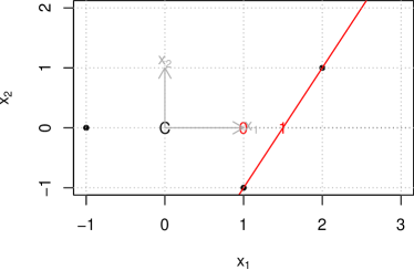
(a) LP (8) with test point on the $x_{1}$-axis: a simple closed-form solution exists.

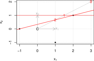
(b) LP (6) on original scale with box constraints: a suboptimal first solution results.

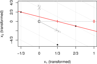
(c) LP (8) on transformed scale and without box constraints: intersection point is found immediately.

Figure 1: A toy example with three points. The centroid is marked with C; arrows indicate standard basis vectors in each dimension on the original scale, target set points are dots, supporting lines are colored red, the initial test point is 0, and its successive iterations are labeled with integers.

To make the example more concrete, let us take $a=2$ and $b=1$. Then, we see in Figure 1a that $\bm{p}=\bm{e}_{1}$ (labeled with 0) is in the convex hull, and, furthermore, that the $x_{1}$ coordinate of the point of intersection is $(2+1)/2=3/2$, and the separating line’s location does not depend where, along the ray from the origin, $\bm{p}$ is. Now, instead, let $\bm{p}$ equal $(3,2){{}^{\top}}$. This is the situation depicted in Figure 1b. The original LP (6), which includes box constraints, finds one separating line—in two dimensions, a hyperplane is a line—but the intersection of this line and the segment connecting $\bm{0}$ to $\bm{p}$, labeled with the digit 1, is not optimal. A second application of LP (6) finds the optimal point labeled 2. In this case, point 2 lies on the line $\{\bm{x}:1+x_{1}+3x_{2}=0\}$, and it is instructive that the box constraints alone prevent LP (6) from finding this solution when $\bm{p}=(3,2){{}^{\top}}$ but not when $\bm{p}=(3/2,1){{}^{\top}}$, where the latter point is the intermediate point labeled 1 in Figure 1b.

Lastly, we illustrate the linear transformation of the previous problem by ${R}$. Figure 1c shows the problem transformed using (7), with the dotted lines and arrows showing the original coordinate system, then LP (8) is applied to find the intersection point in one iteration.

5.2 Benchmarking Rglpk against lpSolveAPI

Here, we define two simple functions that each use LP (9) to search for the point on the ray from $\bm{0}$ through $\bm{p}$ that intersects the boundary of $\overline{\mathcal{C}({M})}$. Each of these functions exploits an existing R package that wraps open-source code solving linear programs: respectively, Rglpk (Theussl and Hornik, 2019) wraps the GNU Linear Programming Kit (GLPK) (Makhorin et al., 2020) and lpSolveAPI (lp_solve et al., 2020) wraps the lp_solve library (Berkelaar et al., 2021). Here is a function that uses lpSolveAPI:

library(lpSolveAPI)

LPmod1 <- function(M, p) { # it is assumed the centroid is the zero vector

  lp <- make.lp(n <- nrow(M), d <- ncol(M))

  for (k in seq_len(d)) set.column(lp, k, M[, k])

  set.constr.type(lp, rep(">=", n))

  set.rhs(lp, rep(-1.0, n))

  set.bounds(lp, lower = rep(-Inf, d), upper = rep(Inf, d)) # z unbounded

  set.objfn(lp, p) # objective function is p %*% z

  solve(lp)

  return(get.objective(lp))

}

Similarly, this code uses Rglpk:

library(Rglpk)

LPmod2 <- function(M, p) { # it is assumed the centroid is the zero vector

  n <- nrow(M)

  d <- ncol(M)

  bounds <- list(

    lower = list(ind = seq(d), val = rep(-Inf, d)),

    upper = list(ind = seq(d), val = rep(Inf, d))

  )

  ans <- Rglpk_solve_LP(

    obj = p, mat = M, dir = rep(">=", n),

    rhs = rep(-1.0, n), bounds = bounds

  )

  return(ans$optimum)

}

A test case simulates $n=100{,}000$ points uniformly distributed in the $d=20$-dimensional unit cube, then verifies that the point $\bm{p}=(1,\dotsc,1){{}^{\top}}$ is not inside the convex hull by finding the smallest $\gamma>0$ such that $\gamma\bm{p}$ is on the boundary:

set.seed(123)

M <- matrix(runif(1e5 * 20), ncol = 20)

Mbar <- colMeans(M)

M <- sweep(M, 2, Mbar) # Translate M so sample mean is at origin

p <- rep.int(1, 20) - Mbar

lpstime <- system.time(lpsstep <- -1 / LPmod1(M, p))[1]

glpktime <- system.time(glpkstep <- -1 / LPmod2(M, p))[1]

stopifnot(isTRUE(all.equal(lpsstep, glpkstep)))

Both implementations produce the same result: $\gamma\approx 0.4801$, but Rglpk takes 10 seconds, whereas lpSolveAPI takes 19. However, Rglpk requires GLPK to be installed separately on some platforms; thus, our suggestion for package developers is to check for availability of GLPK on the system and use Rglpk if it is installed.

6 Testing multiple points

As explained at the beginning of Section 2, the approximated difference of log-likelihoods in (5) requires that every $\bm{g}({Z}_{i})\in{S}$ be contained in ${\mathcal{C}({T})}$ in order for the approximation to have a maximizer. We might therefore consider a strategy of checking, prior to using (5), whether $\bm{g}({Z}_{i})\in{\mathcal{C}({T})}$ for all $i=1,\dotsc,s$ using the single-test-point methods discussed earlier. This strategy has two potential drawbacks: First, the computational burden might be quite high if any of the dimension $d$, the number of test points $s$, or the number of target points $r$ is large. Second, we must decide what to do in the case where one or more of the points in ${S}$ is found to be outside ${\mathcal{C}({T})}$. This section addresses each of these questions and then presents an illustrative example using a network dataset with missing edges.

6.1 Reducing computational burden

There are evidently many possible ways to approach the question of how to efficiently decide which test points, if any, lie outside $\mathcal{C}({T})$. Even if we only consider ideas for reducing the size of the set ${T}$ in such a way as to have little or no influence on the answer, we might attempt to search for and eliminate target set points either that lie entirely inside $\mathcal{C}({T})$, since eliminating such points from ${T}$ does not change $\mathcal{C}({T})$ at all, or that lie close to other points in ${T}$, since eliminating such points does not change $\mathcal{C}({T})$ very much. Here, we merely suggest a simplistic version of the first approach, as a thorough exploration of methods for reducing the size of ${T}$ without altering $\mathcal{C}({T})$ is well beyond the scope of this article.

Whether a point in ${T}$ is interior to $\mathcal{C}({T})$ or whether it lies on the boundary of $\mathcal{C}({T})$ has to do with that point’s so-called data depth, a concept often attributed (in the two-dimensional case) to Tukey (1975). Because the deepest points are the ones that can be eliminated without changing $\mathcal{C}({T})$, the sizable literature on data depth (see, e.g., the discussion by Zuo and Serfling, 2000) may be relevant to our problem. For the $d=2$-dimensional case, several authors have developed efficient methods for identifying exactly the points lying on the convex hull boundary; this is a particular case of the so-called convex layers problem (Chazelle, 1985).

Among the most simplistic ideas is to use Mahalanobis distance from the centroid, defined for any point $\bm{x}\in{T}$ as

$$d(\bm{x})=\sqrt{\bm{x}{{}^{\top}}\hat{\Sigma}^{-1}\bm{x}},$$

where $\hat{\Sigma}$ is the sample covariance matrix, as a measure of data depth. For the $|{T}|=100{,}000$-point example of Section 5.2, we also sample $|{S}|=5$ corners of the unit cube in $\mathbb{R}^{20}$ and try eliminating the fraction $f=i/10$ for $i=1,\dotsc,10$ of the deepest points as measured by Mahalanobis distance:

p <- sweep(matrix(rbinom(5 * 20, 1, 0.5), ncol = 20), 2, Mbar)

d <- rowSums((M %*% solve(cov(M))) * M) # Find squared Mahalanobis distances

M <- M[order(d, decreasing = TRUE), ]

b <- rep(Inf, 10) # Vector for storing LP minima

for (i in 10:1) {

  for (j in 1:nrow(p)) {

    b[i] <- min(b[i], LPmod2(M[1:(i * nrow(M) / 10), ], p[j, ]))

  }

}

Figure 2: In this example where $d=20$ and $n=100{,}000$, half of the target set can be eliminated using a simplistic Mahalonobis distance-based algorithm without appreciably degrading the quality of the convex hull scaling factor.

In this 20-dimensional problem, we see that we can effectively disregard half the points in ${T}$, using a simple Mahalanobis ordering, without degrading the solution appreciably. Since computing effort scales linearly with the number of points in ${T}$, this seems like a useful tool. We nonetheless recommend caution, as our experiments indicate that the fraction of points that may be discarded by their Mahalanobis distances varies considerably for different choices of $d$. For example, we find for $d=50$ that each of the $100{,}000$ points sampled uniformly randomly in the unit cube lies on the boundary of the convex hull.

6.2 Rescaling observed statistics

Recalling the case of a completely observed network, where ${S}$ consists of a single point $\bm{g}({Y}_{\text{obs}})$, the strategy used by Hummel et al. (2012) is to find a point, say $\hat{\bm{\xi}}$, between $\bm{0}$ and $\bm{g}({Y}_{\text{obs}})$ that lies inside $\mathcal{C}({T})$ yet close to the boundary. By treating $\hat{\bm{\xi}}$ as though it is $\bm{g}({Y}_{\text{obs}})$ in constructing approximation (3), the approximation will have a well-defined maximizer, and this maximizer is then used to generate a new target set in the next iteration of the algorithm.

In analogous fashion, when ${S}$ consists of multiple points and some of them lie outside $\mathcal{C}({T})$, we propose to shrink each of these points toward $\bm{0}$ using the same scaling factor, say $\gamma$, where $\gamma\in(0,1]$ is chosen so that every element of ${S}$ lies within $\mathcal{C}({T})$ after the scaling is applied. Since LP (9) yields the optimal step length for each point $\bm{p}$, we obtain this step length by iterating through the points in ${S}$ and selecting the least of the resulting step lengths. This transformation also has the effect of shifting the sample mean of the points in ${S}$ to a point somewhere between $\bm{0}$ and the sample mean of the untransformed points in ${S}$.

6.3 Example

This section illustrates the idea of Section 6.2 using a network representing a school friendship network based on a school community in the rural western United States. The synthetic faux.mesa.high network in the ergm package includes 205 students in grades 7 through 12. We may create a copy of this network and then randomly select 10% of the edge observations (whether the edge is present or absent) to be categorized as missing:

library(ergm)

data(faux.mesa.high)

fmh <- faux.mesa.high

m <- as.matrix(fmh)

el <- cbind(row(m)[lower.tri(m)], col(m)[lower.tri(m)])

set.seed(123)

s <- sample(nrow(el), round(nrow(el) * 0.1))

fmh[el[s, ]] <- NA

If we now define an ERGM using a few statistics related to those originally used to create the faux.mesa.high network—details are found via help(faux.mesa.high)—we begin with an estimator that can be derived using straightforward logistic regression. We denote this maximum pseudo-likelihood estimator or MPLE, details of which may be found in Section 5.2 of Hunter et al. (2008), by theta0 or $\bm{\theta}_{0}$.

fmhFormula <- fmh ~ edges + nodematch("Grade") +

  gwesp(log(3 / 2), fixed = TRUE)

theta0 <- coef(ergm(fmhFormula, estimate = "MPLE"))

To construct approximation (5), we need two samples of random networks, ${Y}_{1},\dotsc,{Y}_{r}$ and ${Z}_{1},\dotsc,{Z}_{s}$ from $\mathcal{Y}$ and $\mathcal{Y}({Y}_{\text{obs}})$, respectively. For the latter, we employ the constraints capability of the ergm package.

gY <- simulate(fmhFormula,

  coef = theta0, nsim = 500, output = "stats",

  control = snctrl(MCMC.interval = 1e4)

)

gZ <- simulate(fmhFormula,

  coef = theta0, nsim = 100, output = "stats",

  constraints = ~observed,

  control = snctrl(MCMC.interval = 1e4)

)

We can use the code developed earlier in this article to show that the $\bm{g}({Z}_{j})$ statistics are not interior to the convex hull of the $\bm{g}({Y}_{i})$ statistics:

centroid <- colMeans(gY)

gY <- sweep(gY, 2, centroid) # Translate the g(Y) statistics

gZ <- sweep(gZ, 2, centroid) # Translate the g(Y) statistics

scale <- Inf

for (j in 1:nrow(gZ)) {

  scale <- min(scale, -1 / LPmod2(gY, gZ[j, ]))

}

The code above finds that 0.733 is the largest scaling factor that, when multiplied by each $\bm{g}({Z}_{j})$ vector, ensures that the result is on or inside the boundary of the convex hull of the target points $\bm{g}({Y}_{1}),\dotsc,\bm{g}({Y}_{100})$. Since this scaling factor is less than 1, at least one element in the test set lies outside $\mathcal{C}({T})$ and so the approximation in (5) has no maximizer. Figure 3 depicts the target points, the test points, and the test points after scaling by 0.733.

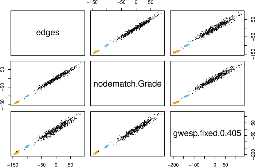
Figure 3: Pairwise scatterplots of three-dimensional network statistics generated using the MPLE, with statistics on the full sample space of networks as black dots and those on the sample space constrained to coincide with the observed network as orange dots. The constrained points are rescaled as blue points so that none lies outside the convex hull of the black points. In each plot, there are 500 black, 100 orange, and 100 blue points.

With our samples in place, we may now construct approximation (5). Here, we negate the function so that our objective is to minimize it:

l <- function(ThetaMinusTheta0, gY, gZ, scale) {

  -log(mean(exp(scale * gZ %*% ThetaMinusTheta0))) +

    log(mean(exp(gY %*% ThetaMinusTheta0)))

}

Finally, we employ the optim function in R (R Core Team, 2021) to minimize the objective function. We use a scale value of 90%  of the value that places one of the test values exactly on the boundary of the convex hull so that all of the scaled test points are interior to the convex hull. We may repeat the whole process iteratively until the entire set of test points is well within the convex hull boundary:

multipliers <- scale

NewTheta <- theta0

while (scale < 1.11) { # We want 0.9 * scale > 1 when finished

  NewTheta <- NewTheta + optim(0 * NewTheta, l,

    gY = gY, gZ = gZ,

    scale = 0.9 * scale

  )$par

  theta0 <- rbind(theta0, NewTheta)

  gY <- simulate(fmhFormula,

    coef = NewTheta, nsim = 500, output = "stats",

    control = snctrl(MCMC.interval = 1e4)

  )

  gZ <- simulate(fmhFormula,

    coef = NewTheta, nsim = 100, output = "stats",

    constraints = ~observed,

    control = snctrl(MCMC.interval = 1e4)

  )

  centroid <- colMeans(gY)

  gY <- sweep(gY, 2, centroid) # Translate the g(Y) statistics

  gZ <- sweep(gZ, 2, centroid) # Translate the g(Y) statistics

  scale <- Inf

  for (j in 1:nrow(gZ)) {

    scale <- min(scale, -1 / LPmod2(gY, gZ[j, ]))

  }

  multipliers <- c(multipliers, scale)

}

Table 1 gives successive values of $\bm{\theta}_{0}$ that are determined as maximizers of (5) after the test set points $\bm{g}({Z}_{1}),\dotsc,\bm{g}({Z}_{s})$ are rescaled to lie within the convex hull of $\bm{g}({Y}_{1}),\dotsc,\bm{g}({Y}_{r})$. The maximum pseudo-likelihood estimate (MPLE) in the first row of the table is obtained using logistic regression and is often used as an initial approximation to the maximum likelihood estimator when employing MCMC MLE (Hunter et al., 2008). However, the MPLE fails to take the missing network observations into account and, as demonstrated by Hummel et al. (2012), it is not the case that the MPLE generates sample network statistics near the observed statistics.

Table 1: Values of theta0 and their associated test point mulipliers, starting with the maximum pseudo-likelihood estimator.

Iteration	edges	nodematch.Grade	gwesp.fixed.0.405	Multiplier
0	-6.302	2.264	1.249	0.733
1	-6.236	2.098	1.276	1.094
2	-6.223	1.981	1.302	2.043

Figure 4 shows that the final value of $\bm{\theta}_{0}$ produces samples such that the whole test set lies on the interior of the target set, which allows (5) to be maximized to produce an approximate MLE. As recommended by Hummel et al. (2012), we might use moderate-sized samples to obtain a viable $\bm{\theta}_{0}$ value using the idea here, then use much larger samples once $\bm{\theta}_{0}$ has been found in order to improve the accuracy of Approximation (5).

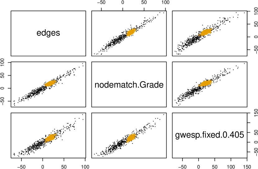
Figure 4: At the final iteration, the test set (orange) is entirely within the convex hull of the target set (black).

7 Discussion

This article discusses the problem of determining whether a given point, or set of points, lies within the convex hull of another set of points in $d$ dimensions. While this problem, along with its solution via linear programming, is known, we are not aware of any work that discusses it in the context of a statistical problem such as one discussed here, namely, the maximization of an approximation to the loglikelihood function for an intractable exponential-family model.

Here, we provide multiple improvements on the simplistic implementation of the linear programming solution to the yes-or-no question involving a single test point that exists in the ergm package (Hunter et al., 2008) as a means of implementing the idea of Hummel et al. (2012): First, we eliminate the need for the “box constraints” of ergm and show how the dual linear program may be derived from first principles. Second, we render the “trial-and-error” approach obsolete by showing how to find the exact point of intersection between the convex hull boundary and the ray originating at the origin and passing through the test point. Third, we test the lpSolveAPI package that is currently used by ergm against the Rglpk package, finding that the latter appears to be far more efficient at solving the particular linear programs we encounter. Fourth, we discuss the statistical case of missing network observations, in which the test set may consist of multiple points, establish an important necessary condition, and suggest a method for handling this case.

In addition, we point out several ways in which this work might be extended, particularly in the case of multiple test points. For one, the question of how to streamline computations is wide open, particularly since it is not necessary to find the exact maximum scaling factor that maps each test point into the convex hull. For the purposes of approximating a maximum likelihood estimator, we seek only an upper bound on the acceptable scaling factors; indeed, in practice we want to scale all test points so that they are inside the boundary. This means that it might be possible to eliminate from the target set any points that are sufficiently close to another target set point and that doing so would not change the needed scaling factor too much.

We might also consider how to optimize the size of the sample chosen for the test set in the first place. For instance, if the scaling factor needed is considerably smaller than one, there might be an advantage in sampling just a handful of points, possibly just a single point in order to move the initial value of $\bm{\theta}_{0}$ closer to the true MLE, when a larger sample of test points could be drawn.

One thing that is clear is that the extensions described here would be much more difficult, if not impossible, to consider without the improvements to the ergm package’s convex-hull testing procedure outlined in this article.

References

- Barndorff-Nielsen (1978) Ole E. Barndorff-Nielsen. Information and Exponential Families in Statistical Theory. Wiley, New York, 1978.
- Berkelaar et al. (2021) Michel Berkelaar, Jeroen Dirks, et al. lp_solve reference guide, 2021. URL https://lpsolve.sourceforge.net/5.5/.
- Besag (1974) Julian Besag. Spatial interaction and the statistical analysis of lattice systems (with discussion). Journal of the Royal Statistical Society, Series B, 36:192–236, 1974.
- Chazelle (1985) Bernard Chazelle. On the convex layers of a planar set. IEEE Transactions on Information Theory, 31(4):509–517, 1985. doi:10.1109/tit.1985.1057060.
- Frank and Strauss (1986) Ove Frank and David Strauss. Markov graphs. Journal of the American Statistical Association, 81(395):832–842, 1986. doi:10.1080/01621459.1986.10478342.
- Gelfand and Carlin (1993) Alan E. Gelfand and Bradley P. Carlin. Maximum-likelihood estimation for constrained- or missing-data models. Canadian Journal of Statistics, 21(3):303–311, 1993. doi:10.2307/3315756.
- Geyer (1994) Charles J. Geyer. On the convergence of monte carlo maximum likelihood calculations. Journal of the Royal Statistical Society: Series B, 56(1):261–274, 1994. doi:10.1111/j.2517-6161.1994.tb01976.x.
- Geyer (2009) Charles J. Geyer. Likelihood inference in exponential families and directions of recession. Electronic Journal of Statistics, 3:259–289, 2009. doi:10.1214/08-EJS349.
- Geyer and Thompson (1992) Charles J. Geyer and Elizabeth A. Thompson. Constrained Monte Carlo maximum likelihood for dependent data. Journal of the Royal Statistical Society: Series B, 54(3):657–683, 1992. doi:10.1111/j.2517-6161.1992.tb01443.x.
- Handcock and Gile (2010) Mark S. Handcock and Krista J. Gile. Modeling social networks from sampled data. Annals of Applied Statistics, 4(1):5–25, 2010. doi:10.1214/08-AOAS221.
- Holland and Leinhardt (1981) Paul W. Holland and Samuel Leinhardt. An exponential family of probability distributions for directed graphs. Journal of the American Statistical Association, 76(373):33–65, 1981.
- Hummel et al. (2012) Ruth M. Hummel, David R. Hunter, and Mark S. Handcock. Improving simulation-based algorithms for fitting ERGMs. Journal of Computational and Graphical Statistics, 21(4):920–939, 2012. doi:10.1080/10618600.2012.679224.
- Hunter et al. (2008) David R. Hunter, Mark S. Handcock, Carter T. Butts, Steven M. Goodreau, and Martina Morris. ergm: A package to fit, simulate and diagnose exponential-family models for networks. Journal of Statistical Software, 24(3):1–29, 2008. doi:10.18637/jss.v024.i03.
- Jaynes (1957) Edwin T. Jaynes. Information theory and statistical mechanics. Physical review, 106(4):620–630, 1957. doi:10.1103/physrev.106.620.
- lp_solve et al. (2020) lp_solve, Kjell Konis, and Florian Schwendinger. lpSolveAPI: R Interface to lp_solve Version 5.5.2.0, 2020. URL https://CRAN.R-project.org/package=lpSolveAPI. R package version 5.5.2.0-17.7.
- Makhorin et al. (2020) Andrew O. Makhorin et al. GLPK (GNU Linear Programming Kit), 2020. URL https://www.gnu.org/software/glpk/.
- R Core Team (2021) R Core Team. R: A Language and Environment for Statistical Computing. R Foundation for Statistical Computing, Vienna, Austria, 2021. URL https://www.R-project.org/.
- Robbins and Monro (1951) Herbert Robbins and Sutton Monro. A stochastic approximation method. The Annals of Mathematical Statistics, 22(3):400–407, 1951. doi:10.1214/aoms/1177729586.
- Schweinberger et al. (2020) Michael Schweinberger, Pavel N. Krivitsky, Carter T. Butts, and Jonathan R. Stewart. Exponential-family models of random graphs: Inference in finite, super and infinite population scenarios. Statistical Science, 35(4):627–662, 2020. doi:10.1214/19-STS743.
- Shmueli et al. (2005) Galit Shmueli, Thomas P. Minka, Joseph B. Kadane, Sharad Borle, and Peter Boatwright. A useful distribution for fitting discrete data: Revival of the Conway–Maxwell–Poisson distribution. Journal of the Royal Statistical Society: Series C, 54(1):127–142, 2005. doi:10.1111/j.1467-9876.2005.00474.x.
- Snijders (2002) Tom A. B. Snijders. Markov chain Monte Carlo estimation of exponential random graph models. Journal of Social Structure, 3(2):1–40, 2002.
- Snijders et al. (2006) Tom A. B. Snijders, Philippa E. Pattison, Garry L. Robins, and Mark S. Handcock. New specifications for exponential random graph models. Sociological Methodology, 36(1):99–153, 2006. doi:10.1111/j.1467-9531.2006.00176.x.
- Strauss (1975) David J. Strauss. A model for clustering. Biometrika, 62(2):467–475, 1975. doi:10.1093/biomet/62.2.467.
- Theussl and Hornik (2019) Stefan Theussl and Kurt Hornik. Rglpk: R/GNU Linear Programming Kit Interface, 2019. URL https://CRAN.R-project.org/package=Rglpk. R package version 0.6-4.
- Tukey (1975) John W. Tukey. Mathematics and the picturing of data. In Ralph D. James, editor, Proceedings of the International Congress of Mathematicians, Vancouver, 1974, volume 2, pages 523–531, 1975.
- Vanderbei (1997) Robert J. Vanderbei. Linear Programming: A Modern Integrated Analysis. Kluwer Academic Publishers, Boston, 1997.
- Zuo and Serfling (2000) Yijun Zuo and Robert Serfling. General notions of statistical depth function. The Annals of Statistics, 28(2):461–482, 2000. doi:10.1214/aos/1016218226.