0   

Tractable Boolean and Arithmetic Circuits

Abstract

Tractable Boolean and arithmetic circuits have been studied extensively in AI for over two decades now. These circuits were initially proposed as “compiled objects,” meant to facilitate logical and probabilistic reasoning, as they permit various types of inference to be performed in linear-time and a feed-forward fashion like neural networks. In more recent years, the role of tractable circuits has significantly expanded as they became a computational and semantical backbone for some approaches that aim to integrate knowledge, reasoning and learning. In this article, we review the foundations of tractable circuits and some associated milestones, while focusing on their core properties and techniques that make them particularly useful for the broad aims of neuro-symbolic AI.

1 Introduction

Tractable circuits, both Boolean and arithmetic, have been receiving an increased attention in AI and computer science more broadly. These circuits represent Boolean and real-valued functions, respectively. They are called tractable because they allow one to answer some hard queries about these functions in polytime, typically through a linear-time, feed-forward pass through the circuit structure. The foundations of these circuits have been developed within the area of knowledge compilation, which aims to compile knowledge into tractable representations for the goal of facilitating efficient reasoning. This area of research has a long tradition in AI; see, e.g., [15] and [73, 95, 46, 41, 49, 107, 43]. A turning point, however, has been the work of [46] which presented a comprehensive theory of knowledge compilation based on tractable Boolean circuits, which are deep representations, in contrast to earlier efforts which focused on flat representations based on conjunctive and disjunctive normal forms; see, e.g., [73, 95]. Another turning point has been the work of [36, 37] which employed tractable Boolean circuits in probabilistic reasoning, giving birth to an extensive line of work on tractable arithmetic circuits. The literature on tractable circuits has enjoyed a number of additional and exciting developments over the years, which have broadened and extended their applications from reasoning, to learning and more recently to neuro-symbolic AI; an area that is concerned with integrating neural and symbolic approaches to AI [56, 89, 10]. These developments have also raised key questions, and in some cases confusions, particularly on tractable arithmetic circuits and their relationship to tractable Boolean circuits and the now prevalent technique of weighted model counting [21]. The goal of this article is to discuss the foundations of tractable Boolean and arithmetic circuits, to clarify their relationships, and to highlight some of the key developments that have contributed to the growing interest surrounding tractable circuits today. But first, we find it pertinent to further elaborate on how and why the role of tractable circuits has evolved over the years.

The original motivation behind knowledge compilation and tractable circuits was based on the following observation. In many reasoning tasks, one is typically interested in posing a large number of queries so the (high) cost of offline compilation can be amortized over the large number of online queries. Today, however, tractable circuits are playing a significantly broader role for a number of reasons. First, these circuits have been providing a systematic methodology for computation, particularly for problems beyond NP which include important tasks in probabilistic reasoning and machine learning; see [43] for a recent survey. Second, reasoning with tractable circuits is not only efficient but can almost always be conducted using linear-time algorithms that traverse these circuits in a feed-forward fashion like neural networks. Moreover, tractable circuits are differentiable. In fact, backpropagation has been performed on these circuits, both Boolean [35] and arithmetic [37], as early as two decades ago when the derivatives were first employed in reasoning tasks. These properties of tractable circuits made them very suitable for integration with modern pipelines for machine learning and neuro-symbolic AI; see, for example, [51, 112, 111, 70, 22, 72, 92, 54, 59, 53] where tractable circuits have been recently employed in and/or integrated with neural networks, deep reinforcement learning, Bayesian network classifiers and (deep) probabilistic logic programs. Even the traditional offline/online divide that originally motivated knowledge compilation for reasoning is now being exploited in modern settings as it is aligned with the training/inference divide that governs modern AI systems; see, e.g., [51]. As such, a recent trend has emerged in which tools and techniques that were initially envisioned for reasoning tasks are now being employed to facilitate learning and its integration with knowledge and reasoning. A few additional milestones have contributed to broadening the applications of tractable circuits and their expanded role today. First is the learning of tractable arithmetic circuits from data, starting with [71]; see also [91]. Second is handcrafting the structure of these circuits, which started with [88]. These developments have significantly expanded the utility of tractable circuits as they provided other modes of usage, beyond compilation from models. They also triggered modern treatments of the theory of tractable arithmetic circuits that are independent of compilation, starting with [24] that we shall discuss later. Another milestone is the integration of tractable Boolean and arithmetic circuits, starting with [67], which provided a profound, new formalism for integrating symbolic knowledge into circuits that perform probabilistic reasoning.

This article is organized as follows. We first treat tractable Boolean circuits in Section 2, followed by tractable arithmetic circuits in Section 3. We then discuss algorithms that compile knowledge into tractable circuits in Section 4 and close with some remarks in Section 5. We do not treat the rich subjects of handcrafting and learning (the structure of) tractable arithmetic circuits as this is beyond the scope of this article.

2 Tractable Boolean Circuits

The theory of tractable Boolean circuits is based on Negation Normal Form (NNF) circuits. These are Boolean circuits that have three types of gates: and-gates, or-gates and inverters, except that inverters can only feed from the circuit variables; see figure on the right. NNF circuits are not tractable. However, by imposing certain properties on them we can attain different degrees of tractability. A comprehensive, but now incomplete, treatment of tractable NNF circuits was given in [47], in which these circuits were studied across the two dimensions of tractability and succinctness. As we increase the strength of properties imposed on NNF circuits, their tractability increases by allowing more queries to be performed on them in polytime. This typically comes at the expense of succinctness as the size of circuits gets larger. We will next review some classes of tractable Boolean circuits, with increasingly stronger properties, which will allow us to efficiently solve decision problems (and their functional variants) that are complete for the complexity classes $\mathsf{NP}\subseteq\mathsf{PP}\subseteq\mathsf{NP}^{\mathsf{PP}}\subseteq\mathsf{PP}^{\mathsf{PP}}$; see also [43]. The algorithms for these increasingly complex problems all take time linear in the circuit size, and operate by traversing the circuit in a feed-forward fashion like neural networks. In the following discussion, we will omit inverters from NNF circuits and use $\neg X$ instead to represent an inverted variable $X$.

Decomposability  One of the simplest properties that make NNF circuits tractable is decomposability [34]. According to this property, circuit fragments that feed into an and-gate cannot share variables. Figure 1 illustrates this property by highlighting two fragments (shaded) that feed into an and-gate. The fragment on the left feeds from variables $K$ and $L$. The one on the right feeds from variables $A$ and $P$. NNF circuits that satisfy the decomposability property are known as DNNF circuits. Sat, an $\mathsf{NP}$-complete problem [32], can be decided in linear time on DNNF circuits [34]. In this context, Sat is the problem of deciding whether the circuit has a satisfying input (generates output $1$).

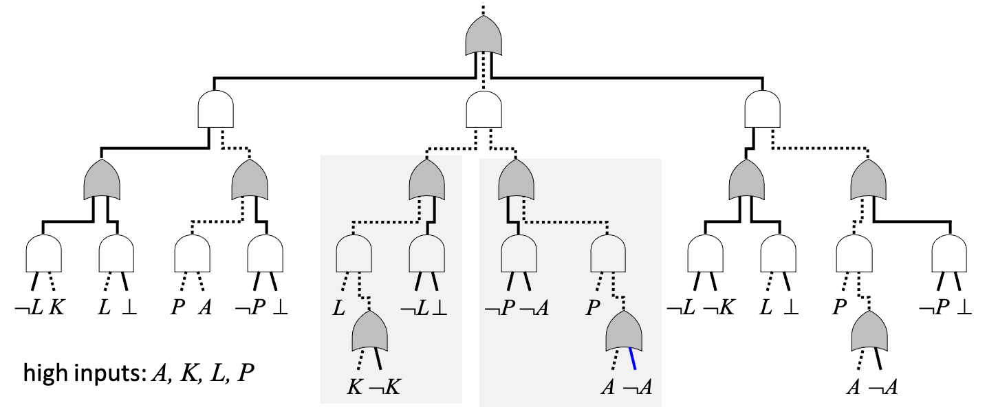
Figure 1: Illustrating the decomposability and determinism properties of NNF circuits. Dotted lines are high wires. Solid lines are low wires. The illustration does not tie shared inputs of the circuit for clarity of exposition.

Determinism  The next property we consider is determinism [35], which applies to or-gates in an NNF circuit. According to this property, at most one input for an or-gate can be high under any circuit input. Figure 1 illustrates this property when all circuit variables $A,K,L,P$ are high. Examining the or-gates in this circuit, under this circuit input, one sees that each or-gate has either one high input or no high inputs. This property corresponds to mutual exclusiveness when an or-gate is viewed as a disjunction of its inputs. NNF circuits that are decomposable and deterministic are known as d-DNNF circuits [35] and they are exponentially less succinct than DNNF circuits [13]. The $\mathsf{PP}$-complete problem MajSat [63] can be decided in polytime on d-DNNF circuits. In this context, MajSat is the problem of deciding whether the majority of circuit inputs satisfy the circuit. If d-DNNF circuits are also smooth [35], a property that can be enforced in quadratic time, these circuits allow one to perform #Sat [108] in linear time; that is, counting the number of satisfying circuit inputs, also known as model counting. If one assigns a weight to each variable value, one can define a weight for each circuit input as the product of weights assigned to its variable values. One can then sum the weights of satisfying circuit inputs also in linear time, a problem that is known as weighted model counting (WMC) [21].

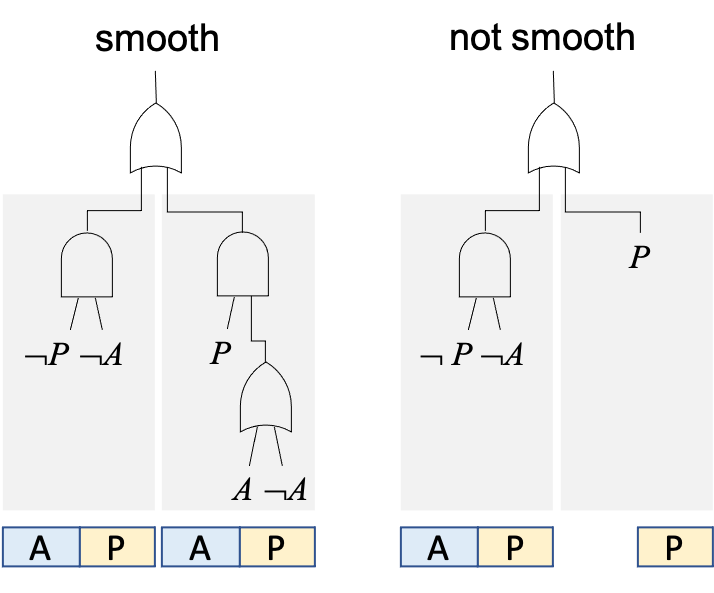
Smoothness  This property requires all circuit fragments feeding into an or-gate to mention the same variables; see illustration on the right. Enforcing smoothness can introduce trivial gates into the circuit, such as the bottom or-gate in the illustration. One can enforce smoothness in quadratic time [35] and sometimes more efficiently [105]. An example of model counting using a d-DNNF circuit is depicted in Figure 2 (left). Every literal in the circuit, whether a positive literal ($A$) or a negative literal ($\neg A$), is assigned the value $1$. Constants $\top$ and $\bot$ are assigned the values $1$ and $0$, respectively. We then propagate these numbers upwards, multiplying numbers assigned to the inputs of an and-gate and summing numbers assigned to the inputs of an or-gate. The number we obtain for the circuit output is the model count. In this example, the circuit has $9$ satisfying inputs out of $16$ possible ones. We can also obtain model counts under variable settings in linear time. For example, if we wish to count the number of satisfying circuit inputs in which ${A\!=\!1}$ and ${K\!=\!0}$, we simply assign $0$ to literals $\neg A$ and $K$ instead of $1$ and then propagate counts as just discussed. This is illustrated in Figure 2 (right), which shows that $2$ out of the $9$ satisfying circuit inputs have ${A\!=\!1}$ and ${K\!=\!0}$. If our goal is to find the model counts under each setting of a single variable, then all such counts can be obtained using a second pass on the smooth d-DNNF circuit. This pass performs backpropagation to compute partial derivatives which can be used to obtain these counts [35]. To perform weighted model counting, we simply assign a weight to a literal instead of the value $1$ and propagate the counts as usual. Model counting is a special case of weighted model counting when each literal weight is $1$.

Figure 2: Model counting through linear-time circuit traversal. Left: counting the number of satisfying circuit inputs. Right: counting the number of satisfying circuit inputs with ${A\!=\!1}$ and ${K\!=\!0}$. Unsatisfiable subscircuits always generate a count of $0$ even if not smooth, so we can exclude them when checking smoothness.

Decision  There are stronger versions of decomposability and determinism which give rise to additional, tractable NNF circuits. A stronger version of determinism is known as the decision property. It requires each or-gate $g$ to have the form $g=(X\wedge\alpha)\vee(\neg X\wedge\beta)$, where $X$ is a circuit variable known as the decision variable of gate $g$ (this or-gate will then satisfy the determinism property). NNF circuits that satisfy decomposability and decision are known as Decision-DNNF circuits [61] and they are exponentially less succinct than d-DNNF circuits [35, 7]. Suppose we split the circuit variables into ${\mathbf{X}}$ and ${\mathbf{Y}}$. We will say that the Decision-DNNF is ${\mathbf{X}}$-constrained iff no or-gate with a decision variable in ${\mathbf{X}}$ can appear below an or-gate with a decision variable in ${\mathbf{Y}}$ [87]. These circuits allow us to solve E-MajSat and its functional variant in time linear in the circuit size. E-MajSat is a decision problem that is $\mathsf{NP}^{\mathsf{PP}}$-complete [110]. It asks: is there an instantiation ${\mathbf{x}}$ under which the majority of instantiations ${\mathbf{y}}$ yield a satisfying circuit input ${\mathbf{x}}{\mathbf{y}}$? The functional version of E-MajSat includes the computation of most likely partial instantiations in probabilistic reasoning [81, 87]. The corresponding feed-forward algorithm performs summation at or-gates with decision variables in ${\mathbf{Y}}$, maximization at or-gates with decision variables in ${\mathbf{X}}$, and multiplication at and-gates [87].

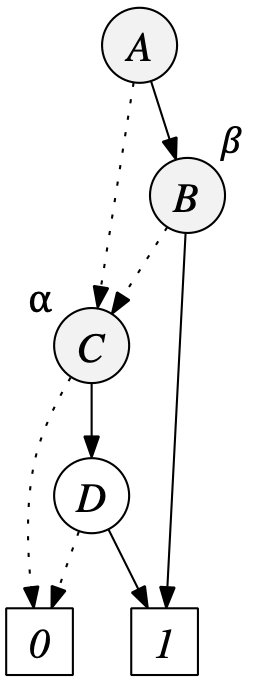
Ordered Binary Decision Diagrams (OBDDs) [14] are perhaps one of the most studied, tractable representations of Boolean functions. OBDDs are a special case of Decision-DNNF circuits even though they are notated differently as shown on the right. Each internal node in an OBDD is labeled with a variable and has two outgoing edges: a low edges (usually dotted) and a high edge (usually solid). The leaf nodes of an OBDD are labeled with $0$ ($\bot$) or $1$ ($\top$). Variables must follow the same order on any path from the root to a leaf in an OBDD. Consider the root node in the OBDD on the right, which is labeled with variable $A$. This node has a low child $\alpha$ and a high child $\beta$. If we replace this node with the or-gate $(\neg A\wedge\alpha)\vee(A\wedge\beta)$ and repeat the same process recursively for OBDDs $\alpha$ and $\beta$, we obtain a Decision-DNNF circuit. That is, we obtain an NNF circuit that satisfies the decomposability and decision properties [46]. Free Binary Decision Diagrams (FBDDs) [57] generalize OBDDs by relaxing the variable ordering requirement while keeping a weaker property known as test-once: each variable must appear at most once on any path from the root to a leaf. FBDDs are also a special case of Decision-DNNF circuits once we adjust for notation and there is a quasipolynomial simulation of Decision-DNNF circuits by equivalent FBDDs [6]. Hence, while FBDDs are less compact than Decision-DNNF circuits, they are not exponentially less succinct. OBDDs are exponentially less succinct than FBDDs though [57] so they are also exponentially less succinct than Decision-DNNF circuits.

Figure 3: Three different types of vtrees: balanced, constrained for $CE|ABD$, and right-linear. A constrained vtree for ${\mathbf{Y}}|{\mathbf{X}}$ is a vtree over variables ${\mathbf{X}}\cup{\mathbf{Y}}$ and contains a unique node $u$ with following properties: (1) $u$ can be reached from the vtree root by following right children only and (2) the variables outside $u$ are precisely ${\mathbf{X}}$. A right-linear vtree is one in which the left child of every internal node is a leaf. A right-linear vtree corresponds to a total variable order ($A,B,C,D,E$ in this case).

Structured Decomposability  This is a stronger version of decomposability which is stated with respect to a full binary tree whose leaves are in one-to-one correspondence with the circuit variables [86]. Three such trees are depicted in Figure 3, which are known as vtrees. Structured decomposability requires each and-gate to have exactly two inputs $i_{1}$ and $i_{2}$, and to have a corresponding node $v$ in the vtree such that the variables of subcircuits feeding into $i_{1}$ and $i_{2}$ are in the left and right subtrees of node $v$. The DNNF circuit in Figure 1 is structured according to the vtree on the left of Figure 3. For example, all and-gates below the root or-gate conform to vtree node $v\!=\!1$ in Figure 3 (left).

Partitioned Determinism  Structured decomposability and a stronger version of determinism, known as partitioned determinism, yield a class of NNF circuits known as Sentential Decision Diagrams (SDDs) [40]. These circuits allow one to solve MajMajSat and its functional variant in linear time. MajMajSat is a decision problem that is $\mathsf{PP}^{\mathsf{PP}}$-complete and is also based on splitting the circuit variables into ${\mathbf{X}}$ and ${\mathbf{Y}}$. It asks: is there a majority of instantiations ${\mathbf{x}}$ under which the majority of instantiations ${\mathbf{y}}$ yield a satisfying circuit input ${\mathbf{x}}{\mathbf{y}}$? The functional variant of MajMajSat includes the computation of expectations such as [31]. To illustrate partitioned determinism, consider Figure 4 and the highlighted circuit fragment. This fragment corresponds to the Boolean expression $(p_{1}\wedge s_{1})\vee(p_{2}\wedge s_{2})\vee(p_{3}\wedge s_{3})$, where each $p_{i}$ is called a prime and each $s_{i}$ is called a sub (primes and subs correspond to subcircuits). Partitioned determinism requires that under any circuit input, precisely one prime will be high (i.e., the primes form a partition). In Figure 4, under the given circuit input, prime $p_{2}$ is high while primes $p_{1}$ and $p_{3}$ are low. This means that this circuit fragment, which acts as a multiplexer, is actually passing the value of sub $s_{2}$ while suppressing the values of subs $s_{1}$ and $s_{3}$. As a result, the or-gate in this circuit fragment is guaranteed to be deterministic: at most one input of the or-gate will be high under any circuit input. SDD circuits result from recursively applying this multiplexer construct to a given vtree (the SDD circuit in Figure 4 is structured with respect to the vtree on the left of Figure 3). Recall that MajMajSat, the prototypical problem for the complexity class $\mathsf{PP}^{\mathsf{PP}}$ [110], is stated with respect to a split of circuit variables into ${\mathbf{X}}$ and ${\mathbf{Y}}$. If the vtree is constrained for ${\mathbf{Y}}|{\mathbf{X}}$, then this problem and its functional variant can be solved in linear time on the corresponding SDD [78]. Figure 3 illustrates the concept of a constrained vtree. When an SDD is structured with respect to a right-linear vtree, the result corresponds to an OBDD after adjusting for notation as discussed earlier. Figure 3 illustrates the concept of a right-linear vtree. In this case, every circuit fragment will have the form $(X\wedge\alpha)\vee(\neg X\wedge\beta)$ where literals $X$ and $\neg X$ are primes, and where $\alpha$ and $\beta$ are subs. OBDDs are therefore a subset of both FBDDs and SDDs and they are exponentially less succinct than SDDs [12]. SDDs and FBDDs are not comparable though in terms of succinctness [8, 11].

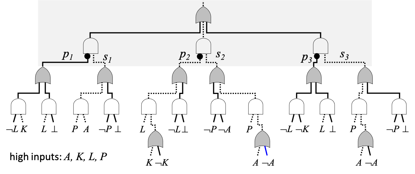
Figure 4: Illustrating the partitioned determinism property of NNF circuits. Dotted lines are high wires. Solid lines are low wires. Precisely one of $p_{1}$, $p_{2}$ and $p_{3}$ will be high for any circuit input.

We have covered in this section only a subset of the tractable Boolean circuits known today, but ones that provide the basis for many of the further refinements and additions; see, e.g, [69] and [96] for some recent additions and [107] for a relatively recent tutorial that covers more circuit types and discusses further the relative succinctness of these circuits. The circuit properties we covered also form a basis for the most influential types of tractable arithmetic circuits. We shall cover these circuit types in the next section.

3 Tractable Arithmetic Circuits

Figure 5: Computing the weighted model count of a tractable Boolean circuit, where $w(\ell)$ represents the weight of literal $\ell$. This computation induces an arithmetic circuit that is superimposed on the Boolean circuit.

We saw in the previous section how counting the models of a tractable Boolean circuit is done through the application of arithmetic operations at Boolean gates: additions at or-gates and multiplications at and-gates. This counting task induces an arithmetic circuit that shares the structure of underlying Boolean circuit as shown in Figure 5, therefore inheriting its properties such as decomposability, determinism and smoothness. Decomposability and smoothness, being structural properties, maintain their exact definitions when moving from the Boolean to the arithmetic side. However, determinism ends up being phrased slightly differently as we shall see later.

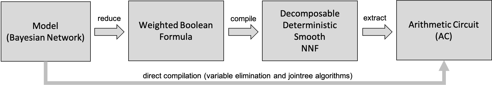
Figure 6: Constructing arithmetic circuits through a compilation process.

The above connection between tractable Boolean and arithmetic circuits originated from [36, 37], which compiled Bayesian networks into tractable arithmetic circuits to enable linear-time probabilistic reasoning on the compiled circuits; see Figure 6. According to this proposal, the Bayesian network is first encoded into a Boolean formula with literal weights, allowing one to reduce probabilistic reasoning into weighted model counting. The Boolean formula is then compiled into a tractable Boolean circuit (deterministic, decomposable and smooth), from which a tractable arithmetic circuit known as an AC is finally extracted. This approach is implemented by the ACE system, which was recently evaluated in [1] and shown to exhibit state-of-the-art performance; see also [52].

A more direct and modern account of tractable arithmetic circuits is given in [24], which reconstructed the proposal in [37] so it is independent of Bayesian networks, model compilation and weighted model counting. This modern treatment was motivated by two influential lines of developments. The first line, which started with [71], utilized arithmetic circuits in the context of learning, in contrast to reasoning. The second line of developments, initiated by [88], handcrafted the structure of arithmetic circuits instead of compiling them from models and dropped the property of determinism while keeping the circuits tractable for certain computations. These developments raised key questions but also broadened the applications of tractable arithmetic circuits significantly. We will next present the modern treatment of [24] which will allow us to also explain more recent classes of tractable arithmetic circuits, such as Sum-Product Networks (SPNs) [88] and Probabilistic Sentential Decision Diagrams (PSDDs) [67]. As we shall see, the treatment in [24] is based on a key distinction between arithmetic circuits, which can lookup values, and tractable arithmetic circuits, which can also reason. As in the Boolean case, the degree to which an arithmetic circuit is tractable and, hence, its ability to conduct various forms of reasoning, depends on the specific properties that the circuit satisfies.

The Reference Point of an Arithmetic Circuit

$A$	$f_{1}$
$a$	$1$
$\bar{{a}}$	$2$

$A$	$B$	$f_{2}$
$a$	$b$	$3$
$a$	$\bar{{b}}$	$4$
$\bar{{a}}$	$b$	$5$
$\bar{{a}}$	$\bar{{b}}$	$6$

$A$	$B$	$f$
$a$	$b$	$3$
$a$	$\bar{{b}}$	$4$
$\bar{{a}}$	$b$	$10$
$\bar{{a}}$	$\bar{{b}}$	$12$

Figure 7: Factors $f_{1}(A)$, $f_{2}(A,B)$, their product factor $f(A,B)=f_{1}f_{2}$, and an arithmetic circuit ${\mathcal{A}C}_{1}$ that computes factor $f(A,B)$. The circuit indicators ($\lambda_{a},\lambda_{\bar{{a}}},\lambda_{b},\lambda_{\bar{{b}}}$) correspond to the values of variables $A$ and $B$. The variables of factors and circuits can be discrete in general (they are binary in this example).

There is a key difference between arithmetic circuits that are compiled from models and those that are handcrafted or learned from data. The former have a clear reference point, the model, which defines the quantities that these circuits are supposed to compute. The latter circuits lack such a reference point which can cause issues when stating and evaluating claims. The theory in [24] starts by defining the reference point of an arithmetic circuit, regardless of where the circuit originates from. This reference point is the notion of a factor: a generalization of a Boolean function that maps complete variable instantiations into non-negative numbers; see Figure 7 (a distribution is one type of a factor).

An arithmetic circuit is based on a set of discrete variables, which define a key ingredient of the circuit: the indicators. For each value $x$ of a variable $X$, we have an indicator $\lambda_{x}$. The arithmetic circuit will then have constants and indicators as its leaf nodes (inputs) with adders and multipliers as its internal nodes; see Figure 7. The factor of an arithmetic circuit (the reference point) is obtained by evaluating the circuit at complete variable instantiations. To evaluate the circuit at an instantiation ${\mathbf{e}}$, we replace each indicator $\lambda_{x}$ with $1$ if the value $x$ is compatible with instantiation ${\mathbf{e}}$ and with $0$ otherwise [37]. We then evaluate the circuit bottom-up in the standard way. The factor $f(A,B)$ in Figure 7 has four rows which correspond to the four instantiations of variables $A$ and $B$. Evaluating the circuit in this figure at each of these complete instantiations yields a value for each instantiation and therefore defines the reference factor. We say in this case that the arithmetic circuit computes this factor. We also say that this circuit can lookup the values of this factor. For example, in Figure 8 (left), the circuit evaluates to $12$ under the complete variable instantiation ${A\!=\!\bar{{a}}},{B\!=\!\bar{{b}}}$ by setting the indicators to ${\lambda_{a}\!=\!0},{\lambda_{\bar{{a}}}\!=\!1},{\lambda_{b}\!=\!0},{\lambda_{\bar{{b}}}\!=\!1}$. An arithmetic circuit can be evaluated at a partial variable instantiation using the same procedure, but the value returned may not be meaningful unless the circuit is tractable (i.e., unless the circuit satisfies certain properties). For example, Figure 8 (right) evaluates the circuit at partial instantiation ${A\!=\!a}$ by setting the indicators to ${\lambda_{a}\!=\!1},{\lambda_{\bar{{a}}}\!=\!0},{\lambda_{b}\!=\!1},{\lambda_{\bar{{b}}}\!=\!1}$, leading to a value of $8$. However, this value is not meaningful since the circuit is not tractable so it cannot reason about the factor. This is a subject that we shall discuss in depth next.

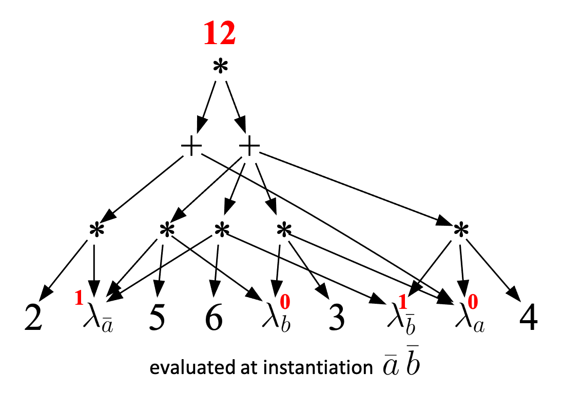
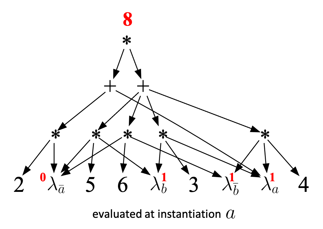
Figure 8: An arithmetic circuit ${\mathcal{A}C}_{1}$ evaluated at complete variable instantiation ${A\!=\!\bar{{a}}},{B\!=\!\bar{{b}}}$ and partial variable instantiation ${A\!=\!a}$. This circuit computes factor $f(A,B)$ in Figure 7: it can lookup the values of factor $f$. This circuit is not decomposable but is smooth and deterministic.

Circuits that Lookup Values Versus Circuits that Reason

The central question posed and treated in [24] is the following. Suppose we have an arithmetic circuit that computes a factor (i.e., looks up its values). Can this circuit reason about the factor and why? Constructing an arithmetic circuit that computes a factor can be done efficiently even when the factor is defined implicitly as a product of other factors (e.g., when the factor is defined by a probabilistic graphical model). Consider the factors and arithmetic circuit in Figure 7. Factor $f(A,B)$ is the product of factors $f_{1}(A)$ and $f_{2}(A,B)$. The arithmetic circuit computes factor $f(A,B)$ and is obtained by multiplying circuits $\lambda_{a}+2\lambda_{\bar{a}}$ and $3\lambda_{a}\lambda_{b}+4\lambda_{a}\lambda_{\bar{b}}+5\lambda_{\bar{a}}\lambda_{b}+6\lambda_{\bar{a}}\lambda_{\bar{b}}$, which compute factors $f_{1}(A)$ and $f_{2}(A,B)$, respectively. This can always be done and the size of resulting circuit is linear in the size of multiplied factors, not the size of their product which can be exponential.

The interest, however, is in tractable arithmetic circuits that can reason about a factor, not ones that can only look up its values. One fundamental reasoning task is that of computing the value of a partial variable instantiation, known as the marginals (MAR) problem [82]. Another fundamental reasoning task is that of identifying and computing the value of a most likely, complete variable instantiation, known as the MPE problem [82]. For factors that are induced by models such as Bayesian networks, the decision variant of MPE is $\mathrm{NP}$-complete [106], the decision variant of MAR is $\mathrm{PP}$-complete and its functional variant is $\mathsf{\#P}$-complete [90], making these hard reasoning tasks.

Consider again the factor $f(A,B)$ in Figure 7 and the partial instantiation ${A\!=\!a}$. The marginal for this instantiation, $f(a)$, is the sum of values assigned to rows that are compatible with instantiation ${A\!=\!a}$: $f(a)=f(a,b)+f(a,\bar{{b}})=3+4=7$. This computation is quite fundamental as it corresponds to computing marginal probabilities when the factor represents a distribution. Interestingly enough, while the arithmetic circuit ${\mathcal{A}C}_{1}$ of Figure 7 does compute the factor, it does not compute its marginals. That is, it can lookup values of rows but cannot sum them up (i.e., cannot reason). A counterexample is shown on the right of Figure 8, where the circuit evaluates to $8$ instead of $7$ at instantiation ${A\!=\!a}$.

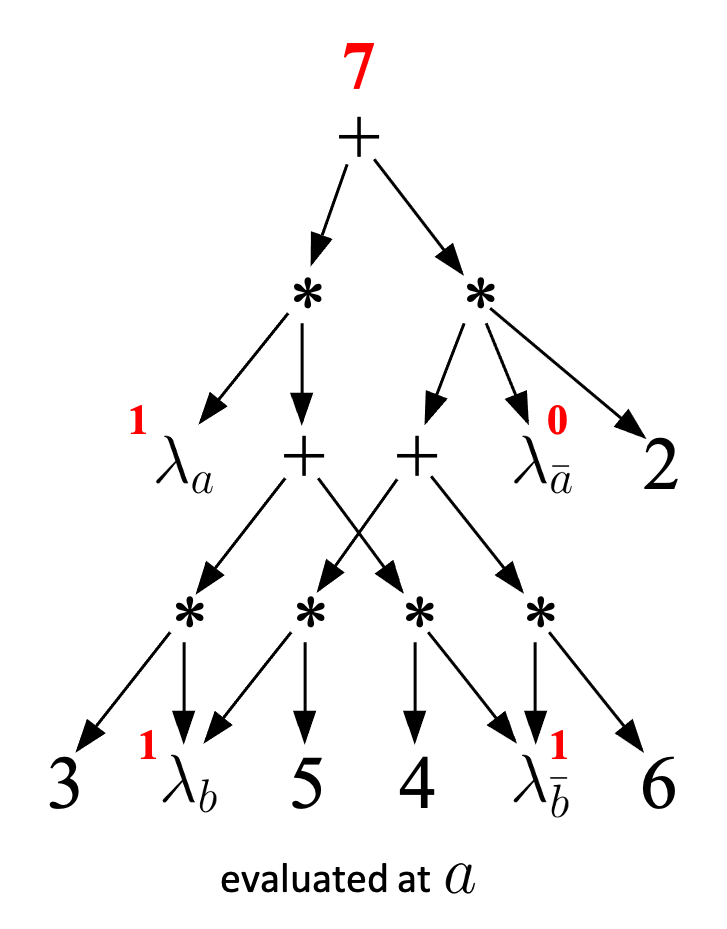
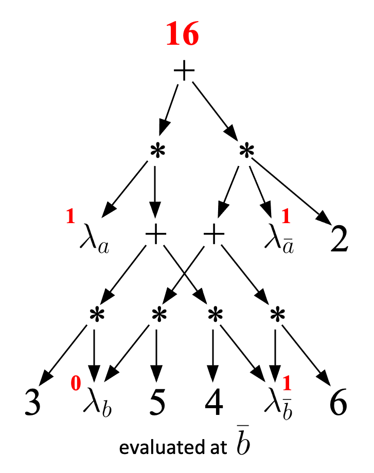
Figure 9: An arithmetic circuit ${\mathcal{A}C}_{2}$, the factor it computes, and evaluations of the circuit under the partial variable instantiations ${A\!=\!a}$ and ${B\!=\!\bar{{b}}}$. This arithmetic circuit computes the factor marginals.

Figure 9 depicts another arithmetic circuit, ${\mathcal{A}C}_{2}$, which computes the same factor computed by ${\mathcal{A}C}_{1}$ of Figure 7. Unlike ${\mathcal{A}C}_{1}$ though, ${\mathcal{A}C}_{2}$ does compute the factor marginals. Figure 9 depicts example evaluations of ${\mathcal{A}C}_{2}$ to be contrasted with the evaluations of ${\mathcal{A}C}_{1}$ in Figure 8. The question now is: Why did ${\mathcal{A}C}_{2}$ compute marginals, and hence reason about the factor, while ${\mathcal{A}C}_{1}$ could not? Before we answer this question, let us first examine another example of reasoning about a factor: computing the value and identity of a most likely, complete variable instantiation (MPE).

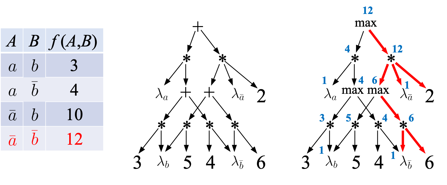
Figure 10: A factor, an arithmetic circuit ${\mathcal{A}C}_{2}$ that computes this factor, and the corresponding maximizer circuit ${\mathcal{M}C}_{2}$. This maximizer circuit computes the factor MPEs.

Consider Figure 10 which depicts ${\mathcal{A}C}_{2}$ again and the factor it computes. The figure shows another circuit, ${\mathcal{M}C}_{2}$, obtained by replacing the adders of ${\mathcal{A}C}_{2}$ with maximizers. This is called a maximizer arithmetic circuit, introduced in [17]. If we evaluate this circuit at the empty variable instantiation by setting all indicators to $1$, we obtain a value of $12$ which is the maximal value attained by any row of the factor; see the right of Figure 10. If we further evaluate this maximizer circuit at instantiation ${B\!=\!b}$, we obtain a value of $10$ which is the maximal value attained by any row of the factor that is compatible with instantiation ${B\!=\!b}$. One can verify that this maximizer circuit will compute the factor MPEs correctly for any variable instantiation, whether complete or partial.

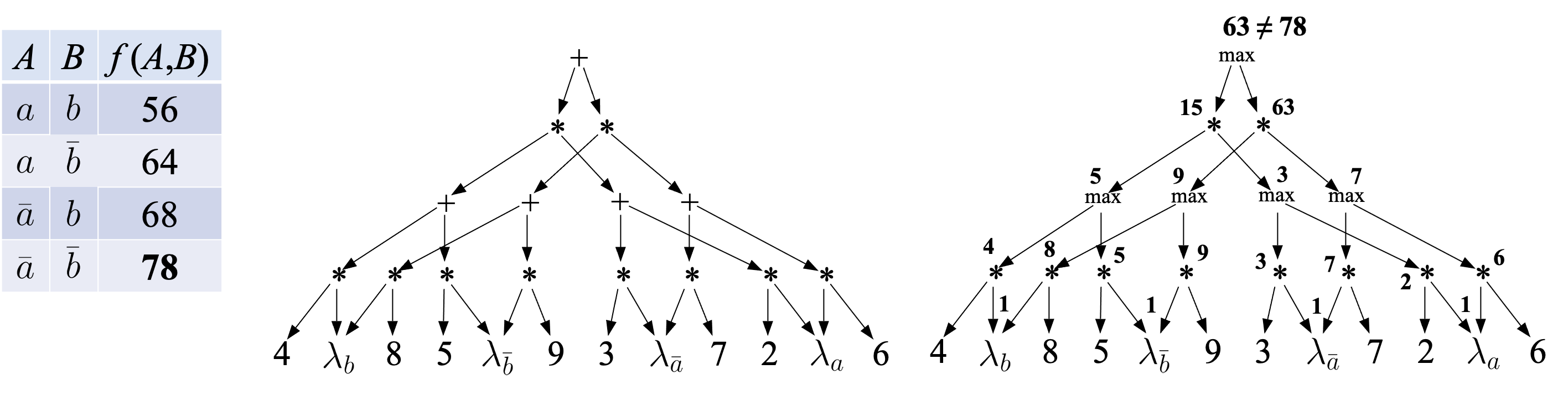
Figure 11: A factor, an arithmetic circuit ${\mathcal{A}C}_{3}$ that computes the factor marginals, and a maximizer circuit ${\mathcal{M}C}_{3}$ that does not compute the factor MPEs.

Consider now Figure 11 which depicts a third arithmetic circuit, ${\mathcal{A}C}_{3}$, and the factor it computes. This circuit computes the factor marginals but does not compute the factor MPEs. The figure shows a counterexample where the maximizer circuit fails to correctly compute the MPE under the empty variable instantiation (all indicators set to $1$). Why did ${\mathcal{M}C}_{3}$ not compute the factor MPEs while ${\mathcal{M}C}_{2}$ did, even though both ${\mathcal{A}C}_{2}$ and ${\mathcal{A}C}_{3}$ compute the marginals of their factors? We are almost ready to address this question, but we first need to introduce another fundamental notion to provide a profound answer.

Complete Subcircuits

Figure 12: Two complete subcircuits (highlighted edges) with their terms and coefficients.

The fundamental notion of a complete subcircuit was first introduced and utilized in [17]. We obtain a complete subcircuit by traversing a circuit top-down. When visiting an adder (or maximizer) node, we choose a single child of the node. When visiting a multiplier node, we choose all its children. Figure 12 depicts two examples. A complete subcircuit has a term and a coefficient. The term is the subscripts of indicators appearing in the subcircuit. The coefficient is the product of numbers appearing in the subcircuit. In Figure 12, the left subcircuit has term $\bar{{a}},\bar{{b}}$ and coefficient $12$. The right subcircuit has term $\bar{{a}},b$ and coefficient $10$. If a maximizer circuit computes the factor MPEs, we can identify a most likely, complete variable instantiation by constructing a complete subcircuit as proposed by [17]. The procedure is simple and illustrated on the right of Figure 10. We traverse the circuit top-down. When visiting a maximizer node, we choose a single child that has the same value as the node. When visiting a multiplier node, we choose all its children. The complete subcircuit selected in Figure 10 has term $\bar{{a}},\bar{{b}}$ and coefficient $12$. This means that $\bar{{a}},\bar{{b}}$ is a most likely, complete variable instantiation and $12$ is its value.

From Lookup to Reasoning: The Source of Tractability

Suppose we have an arithmetic circuit that can lookup factor values (i.e., computes the factor). As discussed earlier, it is generally efficient to construct such circuits (e.g., for the factors specified by probabilistic graphical models). The fundamental question addressed by [24] is the following. Under what conditions, and why, will this circuit attain the ability to reason about the factor (e.g., compute its marginals or compute its MPEs)?

The answer rests in the properties satisfied by the arithmetic circuit: decomposability, determinism and smoothness. We already defined these properties for Boolean circuits. Decomposability and smoothness have identical definitions on arithmetic circuits when viewing adders/multipliers as or/and gates and indicators $\lambda_{x}$ as literals ${X\!=\!x}$. Determinism is defined as having at most one non-zero input for each adder node, when the circuit is evaluated under any complete variable instantiation. We already knew from about two decades ago that if the arithmetic circuit is deterministic, decomposable and smooth, it will compute marginals [37]. We also knew later that such a circuit will compute MPEs [17]. It was further observed about a decade ago that determinism is not needed for computing marginals, leading to a class of arithmetic circuits, known as Sum-Product-Networks (SPNs) [88], which are only decomposable and smooth ([88] referred to smoothness as completeness). We also came to know recently that relaxing determinism can lead to an exponential reduction in the size of an arithmetic circuit [24].

While determinism is not needed for computing factor marginals, it is needed for the correctness of the linear-time MPE algorithm of [17] that we discussed earlier. This was missed in some earlier works [88], which used this algorithm on non-deterministic arithmetic circuits (i.e., SPNs) without realizing that it is no longer correct. This oversight was noticed in later works [84, 74], which also showed the hardness of computing MPEs without determinism [84]. The property of determinism was later called selectivity in the works on SPNs, initially in [83], leading to what has been called Selective SPNs. Since these are arithmetic circuits that satisfy determinism, decomposability and smoothness, they do compute both marginals and MPEs as was already known earlier [37, 17]. As we shall see later, determinism plays another important role even when computing MPE is not of interest as this property allows the compilation of arithmetic circuits from models such as Bayesian networks without the need to search for circuit parameters (constants).

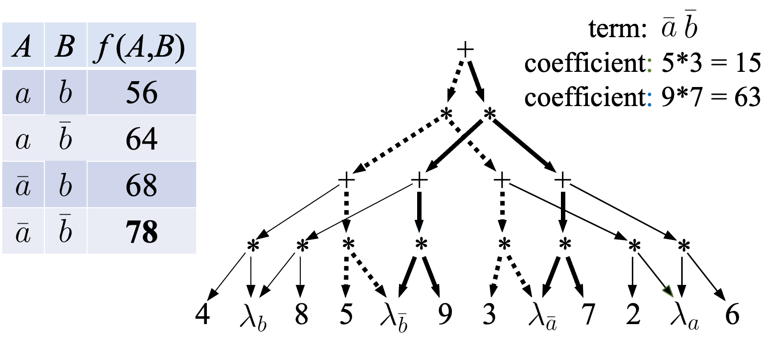
Figure 13: A factor and an arithmetic circuit ${\mathcal{A}C}_{3}$ that computes it. The circuit is decomposable and smooth but not deterministic. The complete subcircuits with term $\bar{{a}},\bar{{b}}$ are highlighted. Their coefficients are $15$ and $63$, which add up to the value $78$ of instantiation $\bar{{a}},\bar{{b}}$.

Some of the key insights provided in [24] related to why the properties of decomposability, determinism, and smoothness make arithmetic circuits tractable, particularly their ability to peform reasoning through linear-time circuit traversal. The fundamental notion here is that of a complete subcircuit which we discussed earlier. Consider Figure 13 which depicts an arithmetic circuit, ${\mathcal{A}C}_{3}$, the factor $f(A,B)$ it computes, and two complete subcircuits of ${\mathcal{A}C}_{3}$. As mentioned earlier, each complete subcircuit has a term ${\mathbf{x}}$ and a coefficient $c$ and will be called an ${\mathbf{x}}$-subcircuit. Both of the highlighted subcircuits in Figure 13 have $\bar{{a}},\bar{{b}}$ as their term and these are the only ($\bar{{a}},\bar{{b}}$)-subcircuits. Their coefficients are $15$ and $63$, which add up to $78$. This is the value assigned by factor $f$ to the variable instantiation $\bar{{a}},\bar{{b}}$, $f(\bar{{a}},\bar{{b}})=78$, which is not a coincidence. As shown in [24], decomposability ensures that the term of a complete subcircuit is consistent: it does not have conflicting variable values. Moreover, smoothness ensures that every variable is instantiated in the term of a complete subcircuit. Hence, decomposability and smoothness ensure that the term ${\mathbf{x}}$ of a complete subcircuit is a complete variable instantiation. Furthermore, for a complete variable instantiation ${\mathbf{x}}$, adding up the coefficients of ${\mathbf{x}}$-subcircuits leads to the value $f({\mathbf{x}})$ assigned by factor $f$ to instantiation ${\mathbf{x}}$. Finally, when evaluating an arithmetic circuit at a partial variable instantiation ${\mathbf{e}}$, the circuit is simply adding up the coefficients of all ${\mathbf{x}}$-subcricuits where ${\mathbf{x}}$ is compatible with ${\mathbf{e}}$, which yields the correct marginal for that instantiation, $f({\mathbf{e}})$ [24]. These results provided the first formal and semantical explanation of why these properties enable an arithmetic circuit that computes a factor to also reason about that factor, therefore making the circuit tractable.

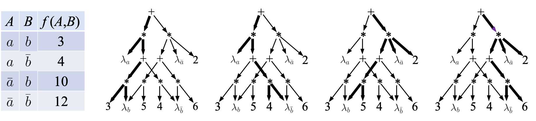
Figure 14: A factor and an arithmetic circuit ${\mathcal{A}C}_{2}$ that computes it. This circuit is decomposable, deterministic and smooth. It has four complete subcircuits, in one-to-one correspondence with the factor rows.

We now get to the property of determinism. As shown in [24], determinism (with decomposability and smoothness) ensures a one-to-one correspondence between complete subcircuits and complete variable instantiations. Moreover, the coefficient $c$ of an ${\mathbf{x}}$-subcircuit corresponds to the value assigned by the factor to complete instantiation ${\mathbf{x}}$: $f({\mathbf{x}})=c$. Figure 14 depicts an arithmetic circuit that is deterministic, decomposable and smooth. This circuit has four complete subcircuits, highlighted in the figure, which are in one-to-one correspondence with the instantiations of variables $A$ and $B$. In the order shown in Figure 14, the subcircuits have terms $a,b;$ $a,\bar{{b}};$ $\bar{{a}},b;$ $\bar{{a}},\bar{{b}}$ and coefficients $3;$ $4;$ $10;$ $12$ which match the rows of the factor computed by the circuit.

What determinism does is ensure that each row of the factor (a complete variable instantiation and its value) is represented by a single, complete subcircuit. This is essential for the linear-time MPE algorithm of [17] to work properly. Consider Figure 11 where this algorithm failed to compute the MPE correctly. The arithmetic circuit in this figure is decomposable and smooth but not deterministic. The MPE (under no evidence) is the complete instantiation $\bar{{a}},\bar{{b}}$ with value $78$. However, this instantiation and its value is not represented by a single, complete subcircuit. Instead, it is represented by two complete subcircuits with coefficients $15$ and $63$ that add up to $78$ as shown in Figure 13. The MPE algorithm will then return the coefficient $63$ as shown in Figure 11, which is not correct.

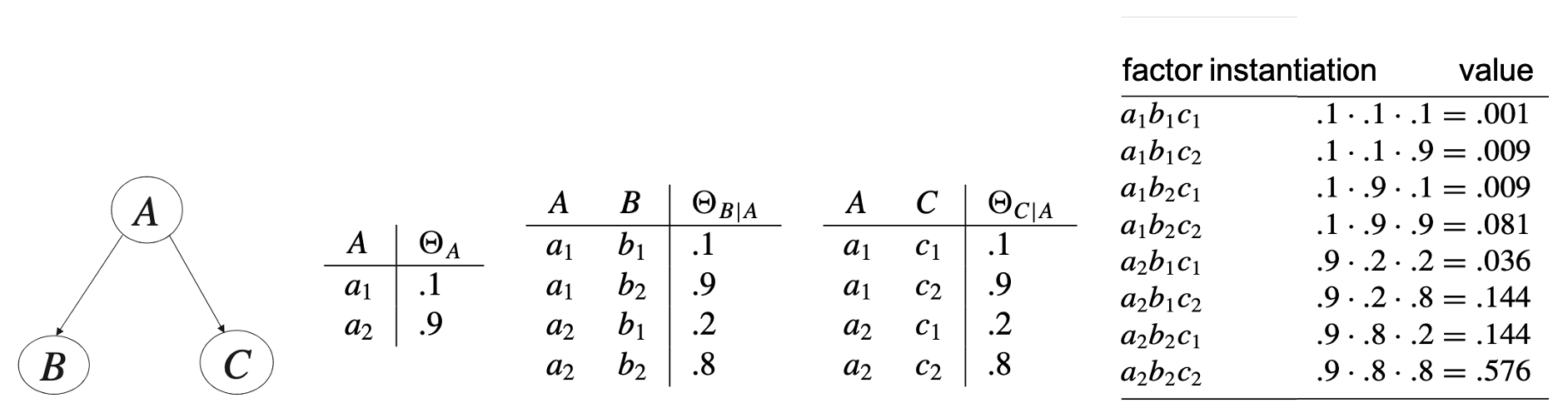
Figure 15: A Bayesian network structure, its conditional probability tables (factors $\Theta_{A}$, $\Theta_{B|A}$, $\Theta_{C|A}$) and the network distribution (factor $f$). The distribution is a product of conditional probability tables, $f=\Theta_{A}\Theta_{B|A}\Theta_{C|A}$.

More on the Need for Determinism

While determinism is not needed for computing marginals, it can be critical for compiling arithmetic circuits from models as we illustrate next. An arithmetic circuit has both a structure and parameters (the constants appearing as circuit inputs). When compiling an arithmetic circuit from a model such as a Bayesian network, one is guaranteed to find a circuit that computes marginals and whose parameters are restricted to the network parameters, if the circuit is deterministic in addition to being decomposable and smooth. However, this guarantee is lost if the circuit is only decomposable and smooth (an SPN) so one must also search for circuit parameters in this case [24]. To elaborate further on this result and its significance, consider the Bayesian network in Figure 15 which has four distinct parameters $\Theta=\{.1,.2,.8,.9\}$. Consider now the distribution (factor $f$) specified by this network. Each value in this factor can be expressed as a product of some parameters that come from $\Theta$ (this is guaranteed by the semantics of Bayesian networks and probabilistic graphical models more generally). We say in this case that the set of parameters $\Theta$ is complete for the factor $f$ (i.e., we can express the values of $f$ using products of numbers from $\Theta$). If a set of parameters $\Theta$ is complete for a factor $f$, there is always an arithmetic circuit that computes factor $f$, that is deterministic, decomposable and smooth, and whose parameters come from the set $\Theta$. Therefore, when constructing (compiling) such a circuit, one does not need to search for circuit parameters beyond the set $\Theta$. This no longer holds without determinism so the compilation process must also search for circuit parameters in addition to its structure—we do not know of any such compilation algorithm today. Consider the Bayesian network in Figure 15 and the following arithmetic circuit which does not require searching for parameters:

$${.001}*\lambda_{a_{1}}*\lambda_{b_{1}}*\lambda_{c_{1}}+{.009}*\lambda_{a_{1}}*\lambda_{b_{1}}*\lambda_{c_{2}}+\ldots+{.576}*\lambda_{a_{2}}*\lambda_{b_{2}}*\lambda_{c_{2}}.$$

This has been called the network polynomial in [37] and the factor polynomial in [24]. Each monomial in this polynomial corresponds to a factor row: its indicators capture the row’s instantiation and its coefficient captures the row’s value (which is a product of Bayesian network parameters). For example, the last monomial ${.576}*\lambda_{a_{2}}*\lambda_{b_{2}}*\lambda_{c_{2}}$ captures instantiation $a_{2},b_{2},c_{2}$ and value $.576=.9*.8*.8$. Viewed as a depth-two arithmetic circuit, this polynomial is deterministic, decomposable and smooth, and all its paramaters come from the Bayesian network parameters. It is also exponentially sized so it is mostly of theoretical interest such as illustrating the result we just discussed. Existing compilation algorithms construct more compact arithmetic circuits without searching for parameters, assuming the model parameters are known. When the model parameters are not known, these algorithms compile arithmetic circuits with symbolic parameters that can be easily replaced with numeric parameters that may be learned from data. This is a topic we shall discuss in Section 4.

It is worth noting that the original treatment of arithmetic circuits in [37] started where our current treatment has ended in the previous paragraph. That is, the starting point of [37] was the notion of a network polynomial which fully captures a distribution. The notion of an arithmetic circuit was then introduced as a tool that can be used to compactly represent the exponentially-sized network polynomial. This formulation was facilitated by the fact that [37] also started by assuming the existence of a model (a Bayesian network), which fully defines the network polynomial. This can no longer be assumed when handcrafting circuits or learning them from data, which prompted the modern treatment in [24]. We finally note that arithmetic circuits which compute distributions and their marginals can be used to reason about uncertain evidence, also called soft evidence, in addition to evidence about continuous variables with local, univariate densities. This can be done by setting the circuit indicators to appropriate real values as discussed in [16] and [39, Section 3.7], respectively.

Circuits that Reason about Constrained Factors

We now turn to a fundamental class of arithmetic circuits, known as PSDDs, which can reason about constrained factors [67]. These are factors in which some rows have fixed zero values so they define mappings from a subset of variable instantiations into non-negative numbers; see Figure 16. Constrained factors, particularly ones representing distributions, have many applications. For example, when learning arithmetic circuits that represent distributions from data, one may have domain knowledge that rules out certain states of the world so we need to ensure that any learned circuit will assign a zero probability to such infeasible states. One may also want to induce or learn distributions over combinatorial (or structured) objects such as total and partial rankings [29], graphs [77], game plays [28], routes on a map [70, 28, 27, 99, 101] and subsets of objects [99]. Distributions over these kind of objects have been captured using constrained factors and reasoned about using PSDDs as done in the works mentioned in the previous sentence.

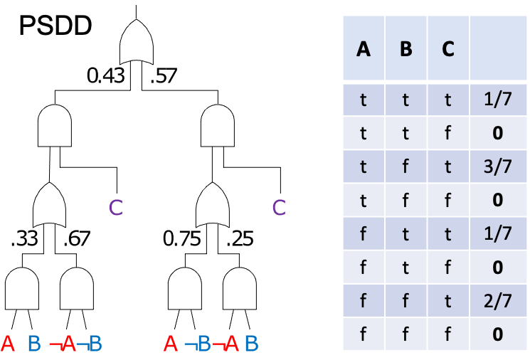
Figure 16: Left: A PSDD and the constrained factor it computes. The factor computed by this PSDD will always assign zero values to rows in which ${C\!=\!f}$, regardless of how the PSDD is parameterized. Right: A PSDD fragment and its corresponding arithmetic circuit fragment. Boolean variables and their negations in the PSDD (e.g., $A$ and $\neg A$) are converted to indicators in the arithmetic circuit ($\lambda_{A}$ and $\lambda_{\neg A}$).

Figure 17: Modeling routes between source $s$ and destination $t$ as variable instantiations that satisfy some conditions. Each edge between two locations is modeled using a Boolean variable which is set to $1$ if the edge is on a route and set to $0$ otherwise. The variable instantiation on the left corresponds to a valid route. The variable instantiation on the right corresponds to an invalid (disconnected) route.

For an example of how constrained factors can be used to model combinatorial and structured objects, consider Figure 17 where the goal is to define a distribution over routes from source $s$ to destination $t$. Each edge on the map is modeled by a binary variable, $A,\ldots,H.$ A route can be modeled using a variable instantiation that sets the variables of its edges to $1$ and all other variables to $0$. Clearly, some variable instantiations do not correspond to valid routes so these get assigned probability $0$; see the right of Figure 17. The corresponding constrained factor is then guaranteed to induce a distribution over only valid routes from source $s$ to destination $t$. Similar techniques can be used to represent other combinatorial or structured objects as long as one can define the conditions that specify variable assignments which correspond to the objects of interest.

A constrained factor is defined by specifying feasible variable instantiations and their values. The main insight behind PSDDs is to specify feasible instantiations using an SDD, which is a tractable Boolean circuit that we discussed in Section 2; see Figure 16 (left). The SDD should evaluate feasible instantiations to $1$ and infeasible instantiations to $0$ and is normally obtained through a compilation process of domain constraints. A distribution over the feasible instantiations can then be defined by assigning (local) distributions to the inputs of or-gates in the SDD, leading to a PSDD as shown in Figure 16.

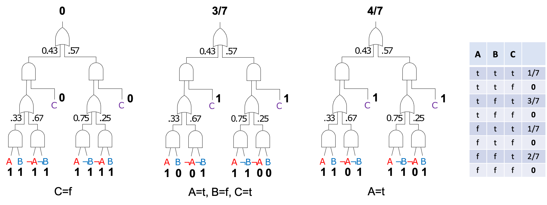
Figure 18: Evaluating a PSDD at different variable instantiations (complete and partial). The PSDD will evaluate to $0$ at any variable instantiations that does not satisfy the underlying SDD circuit. This is guaranteed regardless of how the PSDD is parameterized.

The PSDD is a highly structured arithmetic circuit that comes with strong guarantees. We can convert a PSDD into an arithmetic circuit as shown in Figure 16 (right) by removing reference to the underlying SDD circuit. The resulting arithmetic circuit is guaranteed to not only satisfy determinism, decomposability and smoothness but to also satisfy the stronger properties of structured decomposability and partitioned determinism which are forced by the underlying SDD circuit which satisfies these properties. As a result, the induced arithmetic circuit enjoys many desirable properties. First, the circuit is guaranteed to produce a zero value for any infeasible variable instantiation regardless of how we set the PSDD parameters. Figure 18 depicts example evaluations of a PSDD circuit that can be used to gain insights into this guarantee. Moreover, the PSDD can compute marginals and MPEs by virtue of being deterministic, decomposable and smooth [67]. With an appropriate vtree for the SDD circuit, it can also compute expectations [78]. One can also learn the maximum-likelihood parameters of a PSDD in closed form when the data is complete [67]. An EM algorithm has also been developed for learning PSDD parameters from incomplete data, including highly structured data in which examples can be specified using Boolean constraints, not just variable instantiations [29]. PSDDs also play a key role in probabilistic reasoning as shown in [98].

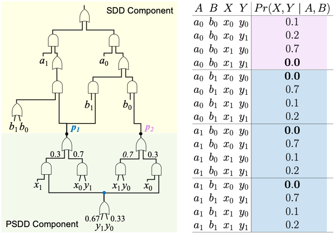
Figure 19: A conditional PSDD composed of an SDD circuit and two PSDDs that share structure. The SDD defines two constrained factors over variables $X$ and $Y$ depending on the state of variables $A$ and $B$. These constrained factors are specified by PSDDs that share structure.

Another key development has been the introduction of conditional PSDDs, which can compute and reason about factors that are conditionally constrained [100]. These are factors in which variables are partitioned into two sets, ${\mathbf{X}}$ and ${\mathbf{Y}}$, where the infeasible instantiations of ${\mathbf{Y}}$-variables are conditioned on the state of ${\mathbf{X}}$-variables. Conditional PSDDs allow one to integrate conditional constraints into tractable arithmetic circuits. For example, which routes are feasible in a neighborhood may be conditional on how we enter and exit that neighborhood [101]. Figure 19 depicts a conditional PSDD, which is composed of an SDD circuit and a set of PSDDs that share structure.

Further Extensions

The theory of tractable arithmetic circuits has been developed and explored in various additional ways. For example, additional classes of arithmetic circuits have been studied using further combinations of tractable circuit properties, such as the combination of structured decomposability and smoothness [33]. Other reasoning tasks have also been considered which are enabled by the different properties of tractable circuits; see, e.g., [109]. Some of the new extensions and works have referred to arithmetic circuits as probabilistic circuits, while reserving the term “arithmetic circuits” to deterministic, decomposable and smooth circuits. This is in contrast to earlier treatments such as [98, 24] which did not tie this term to specific properties or exclusively to probability distributions. A fundamental new extension has been the class of Testing Arithmetic Circuits (TACs) which select their parameters dynamically, based on circuit inputs through the inclusion of tests in the arithmetic circuit [25, 30]. Tractable arithmetic circuits represent multilinear functions (of indicators) [37]. Testing arithmetic circuits represent piecewise multilinear functions so they are universal function approximators like neural networks [30]. This new class of arithmetic circuits can be used to recover from some modeling errors that lead to compiled circuits that may not be expressive enough to fit the data generated by a mechanism that has been modeled incorrectly [102]. Recent theoretical results have shown that full recovery from some modeling errors is possible under certain conditions [60]. We finally note that some of the key properties of tractable circuits, including decomposability and determinism, have been exploited for tractable reasoning and learning in a more general, semiring setting; see, e.g., [65, 66, 55, 9].

4 Compiling Models into Tractable Circuits

We will next provide an overview of methods for constructing tractable circuits through a process of compilation. We will provide a brief summary of methods for tractable Boolean circuits and elaborate more on methods for tractable arithmetic circuits.

Tractable Boolean circuits are normally compiled from Boolean formulas that represent logical knowledge or constraints. This is done using systems known as knowledge compilers, such as D4 [68], c2d [38], CUDD, mini-c2d [79, 80], DSHARP [76] and the SDD library [23]. Knowledge compilers can be categorized as top-down or bottom-up. Top-down compilers are based on keeping a trace of the exhaustive DPLL algorithm [61] and they generally incorporate advanced SAT techniques [93, 80]. These compilers normally operate on Boolean formulas in conjunctive normal form, tend to have better space complexity, and include D4, c2d and DSHARP which yield Decision-DNNFs, and mini-c2d which yields SDDs. Bottom-up compilers incrementally compile a formula, by first compiling its components and then combining these compilations. They tend to operate on more general classes of Boolean formulas, demand more space, and include CUDD and the SDD library, which yield OBDDs and SDDs, respectively.

Turning next to the compilation of tractable arithmetic circuits, we first note that PSDDs, which represent distributions, are somewhat special as these arithmetic circuits are based on SDDs, which are Boolean circuits. Hence, the structure of a PSDD is obtained by first compiling a Boolean formula into an SDD, which is then parameterized to yield a PSDD. The PSDD parameters are typically obtained through a learning process based on complete or incomplete data [67, 29]. The Boolean formula that triggers this compilation process usually defines feasible states of the world, or characterizes structured (combinatorial) objects such as routes, graphs, and rankings.

Arithmetic circuits that satisfy determinism, decomposability and smoothness, also known as ACs, are typically compiled from probabilistic models such as Bayesian networks and probabilistic logic programs. We will only discuss the former but see [72, 54, 53] for some examples of the latter. Recall again that the structure of arithmetic circuits that satisfy only decomposability and smoothness (i.e., SPNs) is normally handcrafted or learned from data since relaxing determinism complicates the compilation of these structures from models as discussed in the previous section.

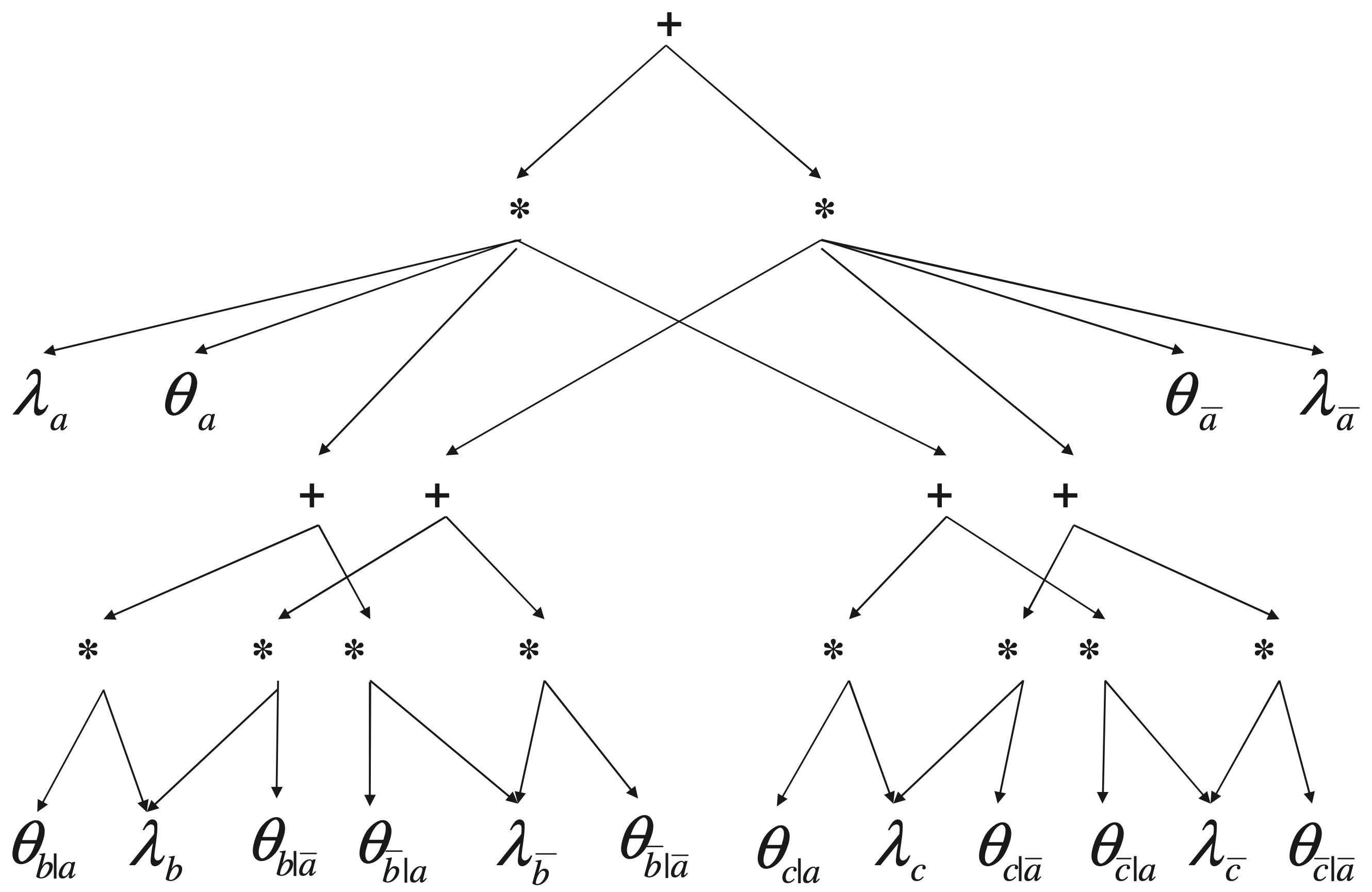
Figure 20: Compiling the Bayesian network $B\leftarrow A\rightarrow C$ into tractable arithmetic circuits. The circuit on the left computes the probability of (partial) evidence on variables $A$, $B$ and $C$. The circuit on the right computes the distribution of variable $B$ given (partial) evidence on variables $A$ and $C$ (after normalization); this circuit targets a particular query, ${\mathit{P}r}(B|.)$. In both cases, the circuit parameters correspond to Bayesian network parameters so they can be fetched from the Bayesian network, if known; otherwise, they can be learned from data.

The compilation of Bayesian networks (and probabilistic graphical models more generally) is done either directly, or indirectly as shown in Figure 6. Indirect methods are based on reductions to weighted model counting [21]. The model is first encoded into a Boolean formula with weights on literals, as initially proposed in [36, 37]. The Boolean formula is then compiled into a smooth d-DNNF circuit (a tractable Boolean circuit), from which a tractable arithmetic circuit is extracted. The size of the final arithmetic circuit depends on the size of compiled Boolean circuit, which is determined by the quality of used encoding scheme and knowledge compiler. These encoding schemes capture both the global structure of the model (its topology) and its local structure (parameters). Their efficacy relies particularly on how well they encode local structure; that is, the extent to which they capture the properties of model parameters. The first encoding scheme [36] was somewhat basic in nature, but it was later followed by more refined and potent encodings in [94, 18, 19]. A comparative discussion of various encoding schemes, including some more recent ones, is given in [52]. The above approaches have traditionally used top-down compilers of Boolean formulas into tractable Boolean circuits; for example, the ACE system [21] used the top-down c2d knowledge compiler. More recently, bottom-up compilation approaches have also been proposed, which are based on compiling the factors of a probabilistic graphical model into tractable circuits and then combining these compiled circuits in a bottom-up fashion [26, 98].

Direct methods for compiling models into tractable arithmetic circuits are simpler but they tend to be less effective, with some exceptions. These methods include the extraction of a tractable arithmetic circuit from the structure of a jointree for the model [37]. They also include methods based on the variable elimination algorithm [20, 42]; see also [39, Chapter 12]. The most recent of these methods [42] is based on variable elimination and stands out for a number of reasons. First, the method compiles circuits that target a specific class of queries, specified by evidence variables (input) and a query variable (output), which is meant to facilities supervised learning from labelled data; see Figure 20. Second, this recent method compiles arithmetic circuits in the form of computation graphs in which nodes represent tensor operations instead of arithmetic operations, allowing parallelization during parameter learning and inference. Third, this method computationally exploites a new type of local structure: functional dependencies whose identities are unknown. We have a functional dependency between a node and its parents in the Bayesian network when the state of the node is a function of the states of its parents (i.e., there is no uncertainty). A functional dependency is unknown when we do not know the identity of this function. This is significant in a learning context where the goal is to learn such functions from data. This is also significant for causal inference where functional dependencies are known as causal mechanisms which are typically unknown [44]. This latest algorithm [42] was motivated by the use of tractable arithmetic circuits for supervised learning, as in neural networks, but where the structure of the circuit is compiled from a model instead of being handcrafted as is normally the case with neural networks. Recent results [22] have shown the promise of this approach to supervised learning as it provides a principled method for embedding background knowledge into the learning process (independence constraints, logical constraints, known parameters, and unknown functional dependencies).

We close this section by the following remark on the interplay between the compilation of circuit structure and the learning of circuit parameters. Initially, the goal of compilation algorithms was to facilitate reasoning since various forms of inference can be performed in linear time on the compiled circuits. In this context, the assumption was that one already knows the model parameters before the compilation process starts. Later, however, these compilation algorithms were used to compile only the circuit structure and then coupled with additional algorithms that learn the circuit parameters from data. The key observation which permits this expanded role is that the compilation process can be conducted even if we do not know the model parameters. In particular, the substitution of model parameters into the compiled circuit can be postponed to the extraction phase of Figure 6. Hence, if a parameter is unknown, it can be kept in symbolic form during the extraction phase and then learned from labeled or unlabeled data after the compilation process is concluded; e.g., as in [42, 22] and [67, 29], respectively. This is possible since determinism (with decomposability and smoothness) allows one to compile circuits with parameters that correspond to model parameters as discussed in the previous section; see also the circuits in Figure 20 and [44] for a recent exposition of how this is done. Interestingly enough, determinism also facilitates the learning of circuit parameters, allowing one to learn parameters in closed form under complete data, in addition to allowing a linear-time evaluation of the EM update equations under incomplete data. This further highlights the importance of determinism, which also holds for tractable arithmetic circuits with handcrafted or learned structures.

5 Concluding Remarks

Tractable Boolean and arithmetic circuits have been evolving into a computational and semantical backbone for modern approaches that aim to combine knowledge, reasoning, and learning. The different modes of constructing these circuits—through compilation, handcrafting and learning—have further contributed to their versatility and positioned them as valuable tools for serving the objectives of neuro-symbolic AI. We provided an overview of tractable circuits in this article, while focusing on their foundations, their salient properties, and some of the key developments and milestones that have contributed to their current status in the field. There is much more to say about tractable circuits beyond what has been covered in this treatment. This includes the various handcrafted architectures, the learning of circuits structures (and parameters) from data, and the compilation of these circuits from higher-level models and other forms of knowledge.

References

- [1] Durgesh Agrawal, Yash Pote, and Kuldeep S. Meel. Partition function estimation: A quantitative study. In IJCAI, pages 4276–4285. ijcai.org, 2021.
- [2] S. Akshay, Jatin Arora, Supratik Chakraborty, Shankara Narayanan Krishna, Divya Raghunathan, and Shetal Shah. Knowledge compilation for Boolean functional synthesis. In FMCAD, pages 161–169. IEEE, 2019.
- [3] Antoine Amarilli. Provenance in databases and links to knowledge compilation. In KOCOON workshop on knowledge compilation, 2019. http://kocoon.gforge.inria.fr/slides/amarilli.pdf.
- [4] Marcelo Arenas, Pablo Barceló Leopoldo Bertossi, and Mikaël Monet. The tractability of shap-score-based explanations over deterministic and decomposable Boolean circuits, 2021.
- [5] Gilles Audemard, Frédéric Koriche, and Pierre Marquis. On tractable XAI queries based on compiled representations. In KR, pages 838–849, 2020.
- [6] Paul Beame, Jerry Li, Sudeepa Roy, and Dan Suciu. Lower bounds for exact model counting and applications in probabilistic databases. In UAI. AUAI Press, 2013.
- [7] Paul Beame, Jerry Li, Sudeepa Roy, and Dan Suciu. Exact model counting of query expressions: Limitations of propositional methods. ACM Trans. Database Syst., 42(1):1:1–1:46, 2017.
- [8] Paul Beame and Vincent Liew. New limits for knowledge compilation and applications to exact model counting. In UAI, pages 131–140. AUAI Press, 2015.
- [9] Vaishak Belle and Luc De Raedt. Semiring programming: A semantic framework for generalized sum product problems. Int. J. Approx. Reason., 126:181–201, 2020.
- [10] Tarek R. Besold, Artur d’Avila Garcez, Sebastian Bader, Howard Bowman, Pedro Domingos, Pascal Hitzler, Kai-Uwe Kuehnberger, Luis C. Lamb, Daniel Lowd, Priscila Machado Vieira Lima, Leo de Penning, Gadi Pinkas, Hoifung Poon, and Gerson Zaverucha. Neural-symbolic learning and reasoning: A survey and interpretation, 2017.
- [11] Beate Bollig and Matthias Buttkus. On the relative succinctness of sentential decision diagrams. Theory Comput. Syst., 63(6):1250–1277, 2019.
- [12] Simone Bova. Sdds are exponentially more succinct than obdds. In AAAI, pages 929–935. AAAI Press, 2016.
- [13] Simone Bova, Florent Capelli, Stefan Mengel, and Friedrich Slivovsky. Knowledge compilation meets communication complexity. In IJCAI, pages 1008–1014. IJCAI/AAAI Press, 2016.
- [14] R. E. Bryant. Graph-based algorithms for Boolean function manipulation. IEEE Transactions on Computers, C-35:677–691, 1986.
- [15] Marco Cadoli and Francesco M. Donini. A survey on knowledge compilation. AI Commun., 10(3-4):137–150, 1997.
- [16] Hei Chan and Adnan Darwiche. On the revision of probabilistic beliefs using uncertain evidence. Artif. Intell., 163(1):67–90, 2005.
- [17] Hei Chan and Adnan Darwiche. On the robustness of most probable explanations. In Proceedings of the 22nd Conference in Uncertainty in Artificial Intelligence (UAI), 2006.
- [18] Mark Chavira and Adnan Darwiche. Compiling Bayesian networks with local structure. In Leslie Pack Kaelbling and Alessandro Saffiotti, editors, IJCAI-05, Proceedings of the Nineteenth International Joint Conference on Artificial Intelligence, pages 1306–1312. Professional Book Center, 2005.
- [19] Mark Chavira and Adnan Darwiche. Encoding cnfs to empower component analysis. In SAT, volume 4121 of Lecture Notes in Computer Science, pages 61–74. Springer, 2006.
- [20] Mark Chavira and Adnan Darwiche. Compiling Bayesian networks using variable elimination. In Proceedings of the 20th International Joint Conference on Artificial Intelligence (IJCAI), pages 2443–2449, 2007.
- [21] Mark Chavira and Adnan Darwiche. On probabilistic inference by weighted model counting. Artif. Intell., 172(6-7):772–799, 2008.
- [22] Yizuo Chen, Arthur Choi, and Adnan Darwiche. Supervised learning with background knowledge. In PGM, volume 138 of Proceedings of Machine Learning Research, pages 89–100. PMLR, 2020.
- [23] Arthur Choi and Adnan Darwiche. Dynamic minimization of sentential decision diagrams. In Proceedings of the 27th Conference on Artificial Intelligence (AAAI), 2013.
- [24] Arthur Choi and Adnan Darwiche. On relaxing determinism in arithmetic circuits. In Proceedings of the Thirty-Fourth International Conference on Machine Learning (ICML), pages 825–833, 2017.
- [25] Arthur Choi and Adnan Darwiche. On the relative expressiveness of Bayesian and neural networks. In PGM, volume 72 of Proceedings of Machine Learning Research, pages 157–168. PMLR, 2018.
- [26] Arthur Choi, Doga Kisa, and Adnan Darwiche. Compiling probabilistic graphical models using sentential decision diagrams. In ECSQARU, volume 7958 of Lecture Notes in Computer Science, pages 121–132. Springer, 2013.
- [27] Arthur Choi, Yujia Shen, and Adnan Darwiche. Tractability in structured probability spaces. In Advances in Neural Information Processing Systems 30 (NIPS), 2017.
- [28] Arthur Choi, Nazgol Tavabi, and Adnan Darwiche. Structured features in naive Bayes classification. In AAAI, 2016.
- [29] Arthur Choi, Guy Van den Broeck, and Adnan Darwiche. Tractable learning for structured probability spaces: A case study in learning preference distributions. In IJCAI, 2015.
- [30] Arthur Choi, Ruocheng Wang, and Adnan Darwiche. On the relative expressiveness of Bayesian and neural networks. Int. J. Approx. Reason., 113:303–323, 2019.
- [31] Arthur Choi, Yexiang Xue, and Adnan Darwiche. Same-decision probability: A confidence measure for threshold-based decisions. Int. J. Approx. Reason., 53(9):1415–1428, 2012.
- [32] Stephen A. Cook. The complexity of theorem-proving procedures. In STOC, pages 151–158. ACM, 1971.
- [33] Meihua Dang, Antonio Vergari, and Guy Van den Broeck. Strudel: Learning structured-decomposable probabilistic circuits. In PGM, volume 138 of Proceedings of Machine Learning Research, pages 137–148. PMLR, 2020.
- [34] Adnan Darwiche. Decomposable negation normal form. J. ACM, 48(4):608–647, 2001.
- [35] Adnan Darwiche. On the tractable counting of theory models and its application to truth maintenance and belief revision. J. Appl. Non Class. Logics, 11(1-2):11–34, 2001.
- [36] Adnan Darwiche. A logical approach to factoring belief networks. In Dieter Fensel, Fausto Giunchiglia, Deborah L. McGuinness, and Mary-Anne Williams, editors, Proceedings of the Eights International Conference on Principles and Knowledge Representation and Reasoning (KR-02), Toulouse, France, April 22-25, 2002, pages 409–420. Morgan Kaufmann, 2002.
- [37] Adnan Darwiche. A differential approach to inference in Bayesian networks. J. ACM, 50(3):280–305, 2003.
- [38] Adnan Darwiche. New Advances in Compiling CNF into Decomposable Negation Normal Form. In ECAI, pages 328–332, 2004.
- [39] Adnan Darwiche. Modeling and Reasoning with Bayesian Networks. Cambridge University Press, 2009.
- [40] Adnan Darwiche. SDD: A new canonical representation of propositional knowledge bases. In IJCAI, pages 819–826. IJCAI/AAAI, 2011.
- [41] Adnan Darwiche. Tractable knowledge representation formalisms. In Tractability: Practical Approaches to Hard Problems, pages 141–172. Cambridge University Press, 2014.
- [42] Adnan Darwiche. An advance on variable elimination with applications to tensor-based computation. In ECAI, volume 325 of Frontiers in Artificial Intelligence and Applications, pages 2559–2568. IOS Press, 2020.
- [43] Adnan Darwiche. Three modern roles for logic in AI. In PODS, pages 229–243. ACM, 2020.
- [44] Adnan Darwiche. Causal inference with tractable circuits. In Why-21 Workshop, NeurIPS, 2021.
- [45] Adnan Darwiche and Auguste Hirth. On the reasons behind decisions. In ECAI, volume 325 of Frontiers in Artificial Intelligence and Applications, pages 712–720. IOS Press, 2020.
- [46] Adnan Darwiche and Pierre Marquis. A knowledge compilation map. J. Artif. Intell. Res., 17:229–264, 2002.
- [47] Adnan Darwiche and Pierre Marquis. A knowledge compilation map. JAIR, 17:229–264, 2002.
- [48] Adnan Darwiche and Pierre Marquis. On quantifying literals in Boolean logic and its applications to explainable AI. CoRR, abs/2108.09876, 2021.
- [49] Adnan Darwiche, Pierre Marquis, Dan Suciu, and Stefan Szeider. Recent trends in knowledge compilation (dagstuhl seminar 17381). Dagstuhl Reports, 7(9):62–85, 2017.
- [50] Guy Van den Broeck, Anton Lykov, Maximilian Schleich, and Dan Suciu. On the tractability of shap explanations, 2021.
- [51] Luca Di Liello, Pierfrancesco Ardino, Jacopo Gobbi, Paolo Morettin, Stefano Teso, and Andrea Passerini. Efficient generation of structured objects with constrained adversarial networks. In H. Larochelle, M. Ranzato, R. Hadsell, M. F. Balcan, and H. Lin, editors, Advances in Neural Information Processing Systems, volume 33, pages 14663–14674. Curran Associates, Inc., 2020.
- [52] Paulius Dilkas and Vaishak Belle. Weighted model counting with conditional weights for Bayesian networks. In UAI, 2021.
- [53] Anton Dries, Angelika Kimmig, Wannes Meert, Joris Renkens, Guy Van den Broeck, Jonas Vlasselaer, and Luc De Raedt. Problog2: Probabilistic logic programming. In ECML/PKDD (3), volume 9286 of Lecture Notes in Computer Science, pages 312–315. Springer, 2015.
- [54] Daan Fierens, Guy Van den Broeck, Joris Renkens, Dimitar Sht. Shterionov, Bernd Gutmann, Ingo Thon, Gerda Janssens, and Luc De Raedt. Inference and learning in probabilistic logic programs using weighted Boolean formulas. Theory Pract. Log. Program., 15(3):358–401, 2015.
- [55] Abram L. Friesen and Pedro M. Domingos. The sum-product theorem: A foundation for learning tractable models. In Proceedings of the 33nd International Conference on Machine Learning (ICML), pages 1909–1918, 2016.
- [56] A. Garcez and L. Lamb. Neurosymbolic ai: The 3rd wave. ArXiv, abs/2012.05876, 2020.
- [57] Jordan Gergov and Christoph Meinel. Efficient boolean manipulation with obdd’s can be extended to fbdd’s. IEEE Trans. Computers, 43(10):1197–1209, 1994.
- [58] Pascal Hitzler and Md Kamruzzaman Sarker, editors. Neuro-Symbolic Artificial Intelligence: The State of the Art, volume 342 of Frontiers in Artificial Intelligence and Applications. IOS Press, 2021.
- [59] Steven Holtzen, Guy Van den Broeck, and Todd D. Millstein. Scaling exact inference for discrete probabilistic programs. Proc. ACM Program. Lang., 4(OOPSLA):140:1–140:31, 2020.
- [60] Haiying Huang and Adnan Darwiche. On recovering from modeling errors using testing Bayesian networks. In ICML, volume 139 of Proceedings of Machine Learning Research, pages 4402–4411. PMLR, 2021.
- [61] Jinbo Huang and Adnan Darwiche. The language of search. J. Artif. Intell. Res., 29:191–219, 2007.
- [62] Xuanxiang Huang, Yacine Izza, Alexey Ignatiev, Martin C. Cooper, Nicholas Asher, and Joao Marques-Silva. Efficient explanations for knowledge compilation languages, 2021.
- [63] John T. Gill III. Computational complexity of probabilistic turing machines. In STOC, pages 91–95. ACM, 1974.
- [64] Abhay Kumar Jha and Dan Suciu. Knowledge compilation meets database theory: Compiling queries to decision diagrams. Theory Comput. Syst., 52(3):403–440, 2013.
- [65] Angelika Kimmig, Guy Van den Broeck, and Luc De Raedt. Algebraic model counting. CoRR, abs/1211.4475, 2012.
- [66] Angelika Kimmig, Guy Van den Broeck, and Luc De Raedt. Algebraic model counting. International Journal of Applied Logic, November 2016.
- [67] Doga Kisa, Guy Van den Broeck, Arthur Choi, and Adnan Darwiche. Probabilistic sentential decision diagrams. In KR. AAAI Press, 2014.
- [68] Jean-Marie Lagniez and Pierre Marquis. An improved decision-dnnf compiler. In IJCAI, pages 667–673. ijcai.org, 2017.
- [69] Yong Lai, Kuldeep S. Meel, and Roland H. C. Yap. The power of literal equivalence in model counting. In AAAI, pages 3851–3859. AAAI Press, 2021.
- [70] Jiajing Ling, Kushagra Chandak, and Akshat Kumar. Integrating knowledge compilation with reinforcement learning for routes. In ICAPS, pages 542–550. AAAI Press, 2021.
- [71] Daniel Lowd and Pedro M. Domingos. Learning arithmetic circuits. In Proceedings of the 24th Conference in Uncertainty in Artificial Intelligence (UAI), pages 383–392, 2008.
- [72] Robin Manhaeve, Sebastijan Dumancic, Angelika Kimmig, Thomas Demeester, and Luc De Raedt. DeepProbLog: Neural probabilistic logic programming. In BNAIC/BENELEARN, volume 2491 of CEUR Workshop Proceedings. CEUR-WS.org, 2019.
- [73] Pierre Marquis. Knowledge compilation using theory prime implicates. In Proceedings of the Fourteenth International Joint Conference on Artificial Intelligence (IJCAI), pages 837–845, 1995.
- [74] Denis Deratani Mauá and Cassio Polpo de Campos. Approximation complexity of maximum a posteriori inference in sum-product networks. CoRR, abs/1703.06045, 2017.
- [75] Alejandro Molina, Antonio Vergari, Karl Stelzner, Robert Peharz, Pranav Subramani, Nicola Di Mauro, Pascal Poupart, and Kristian Kersting. SPFlow: An easy and extensible library for deep probabilistic learning using sum-product networks, 2019.
- [76] Christian J. Muise, Sheila A. McIlraith, J. Christopher Beck, and Eric I. Hsu. Dsharp: Fast d-dnnf compilation with sharpsat. In Canadian Conference on AI, volume 7310 of Lecture Notes in Computer Science, pages 356–361. Springer, 2012.
- [77] Masaaki Nishino, Norihito Yasuda, Shin-ichi Minato, and Masaaki Nagata. Compiling graph substructures into sentential decision diagrams. In Proceedings of the Thirty-First AAAI Conference on Artificial Intelligence, AAAI’17, page 1213–1221. AAAI Press, 2017.
- [78] Umut Oztok, Arthur Choi, and Adnan Darwiche. Solving pp-complete problems using knowledge compilation. In Chitta Baral, James P. Delgrande, and Frank Wolter, editors, Principles of Knowledge Representation and Reasoning: Proceedings of the Fifteenth International Conference, KR 2016, Cape Town, South Africa, April 25-29, 2016, pages 94–103. AAAI Press, 2016.
- [79] Umut Oztok and Adnan Darwiche. On compiling CNF into decision-DNNF. In Proceedings of the 20th International Conference on Principles and Practice of Constraint Programming (CP), pages 42–57, 2014.
- [80] Umut Oztok and Adnan Darwiche. An exhaustive DPLL algorithm for model counting. J. Artif. Intell. Res., 62:1–32, 2018.
- [81] James D. Park and Adnan Darwiche. Complexity results and approximation strategies for MAP explanations. J. Artif. Intell. Res., 21:101–133, 2004.
- [82] Judea Pearl. Probabilistic Reasoning in Intelligent Systems: Networks of Plausible Inference. Morgan Kaufmann, 1988.
- [83] Robert Peharz, Robert Gens, and Pedro M. Domingos. Learning selective sum-product networks. In LTPM workshop, 2014.
- [84] Robert Peharz, Robert Gens, Franz Pernkopf, and Pedro Domingos. On the latent variable interpretation in sum-product networks. IEEE Transactions on Pattern Analysis and Machine Intelligence (TPAMI), 2016.
- [85] Robert Peharz, Steven Lang, Antonio Vergari, Karl Stelzner, Alejandro Molina, Martin Trapp, Guy Van den Broeck, Kristian Kersting, and Zoubin Ghahramani. Einsum networks: Fast and scalable learning of tractable probabilistic circuits. In ICML, volume 119 of Proceedings of Machine Learning Research, pages 7563–7574. PMLR, 2020.
- [86] Knot Pipatsrisawat and Adnan Darwiche. New compilation languages based on structured decomposability. In AAAI, pages 517–522. AAAI Press, 2008.
- [87] Knot Pipatsrisawat and Adnan Darwiche. A New d-DNNF-Based Bound Computation Algorithm for Functional EMAJSAT. In IJCAI, pages 590–595, July 2009.
- [88] Hoifung Poon and Pedro M. Domingos. Sum-product networks: A new deep architecture. In UAI, pages 337–346. AUAI Press, 2011.
- [89] Luc De Raedt, Sebastijan Dumancic, Robin Manhaeve, and Giuseppe Marra. From statistical relational to neuro-symbolic artificial intelligence. In IJCAI, pages 4943–4950. ijcai.org, 2020.
- [90] Dan Roth. On the hardness of approximate reasoning. Artif. Intell., 82(1-2):273–302, 1996.
- [91] Dan Roth and Rajhans Samdani. Learning multi-linear representations of distributions for efficient inference. Mach. Learn., 76(2-3):195–209, 2009.
- [92] Feras A. Saad, Martin C. Rinard, and Vikash K. Mansinghka. SPPL: probabilistic programming with fast exact symbolic inference. In PLDI, pages 804–819. ACM, 2021.
- [93] Tian Sang, Fahiem Bacchus, Paul Beame, Henry A. Kautz, and Toniann Pitassi. Combining component caching and clause learning for effective model counting. In SAT, 2004.
- [94] Tian Sang, Paul Beame, and Henry A. Kautz. Performing Bayesian inference by weighted model counting. In AAAI, pages 475–482. AAAI Press / The MIT Press, 2005.
- [95] Bart Selman and Henry A. Kautz. Knowledge compilation and theory approximation. J. ACM, 43(2):193–224, 1996.
- [96] Preey Shah, Aman Bansal, S. Akshay, and Supratik Chakraborty. A normal form characterization for efficient Boolean skolem function synthesis. In LICS, pages 1–13. IEEE, 2021.
- [97] Shubham Sharma, Rahul Gupta, Subhajit Roy, and Kuldeep S. Meel. Knowledge compilation meets uniform sampling. In LPAR, volume 57 of EPiC Series in Computing, pages 620–636. EasyChair, 2018.
- [98] Yujia Shen, Arthur Choi, and Adnan Darwiche. Tractable operations for arithmetic circuits of probabilistic models. In NIPS, pages 3936–3944, 2016.
- [99] Yujia Shen, Arthur Choi, and Adnan Darwiche. A tractable probabilistic model for subset selection. In Proceedings of the 33rd Conference on Uncertainty in Artificial Intelligence (UAI), 2017.
- [100] Yujia Shen, Arthur Choi, and Adnan Darwiche. Conditional PSDDs: Modeling and learning with modular knowledge. In AAAI, pages 6433–6442. AAAI Press, 2018.
- [101] Yujia Shen, Anchal Goyanka, Adnan Darwiche, and Arthur Choi. Structured Bayesian Networks: From inference to learning with routes. In AAAI, pages 7957–7965. AAAI Press, 2019.
- [102] Yujia Shen, Haiying Huang, Arthur Choi, and Adnan Darwiche. Conditional independence in Testing Bayesian Networks. In ICML, volume 97 of Proceedings of Machine Learning Research, pages 5701–5709. PMLR, 2019.
- [103] Weijia Shi, Andy Shih, Adnan Darwiche, and Arthur Choi. On tractable representations of binary neural networks. In KR, pages 882–892, 2020.
- [104] Andy Shih, Arthur Choi, and Adnan Darwiche. A symbolic approach to explaining Bayesian network classifiers. In IJCAI, pages 5103–5111. ijcai.org, 2018.
- [105] Andy Shih, Guy Van den Broeck, Paul Beame, and Antoine Amarilli. Smoothing structured decomposable circuits. In NeurIPS, pages 11412–11422, 2019.
- [106] Solomon Eyal Shimony. Finding MAPs for belief networks is NP-hard. Artif. Intell., 68(2):399–410, 1994.
- [107] Friedrich Slivovsky. An introduction to knowledge compilation. In KOCOON workshop on knowledge compilation, 2019. http://kocoon.gforge.inria.fr/slides/slivovsky.pdf.
- [108] Leslie G. Valiant. The complexity of enumeration and reliability problems. SIAM J. Comput., 8(3):410–421, 1979.
- [109] Antonio Vergari, YooJung Choi, Anji Liu, Stefano Teso, and Guy Van den Broeck. A compositional atlas of tractable circuit operations: From simple transformations to complex information-theoretic queries. CoRR, abs/2102.06137, 2021.
- [110] Klaus W. Wagner. The complexity of combinatorial problems with succinct input representation. Acta Informatica, 23(3):325–356, 1986.
- [111] Yaqi Xie, Ziwei Xu, Kuldeep S. Meel, Mohan S. Kankanhalli, and Harold Soh. Embedding symbolic knowledge into deep networks. In NeurIPS, pages 4235–4245, 2019.
- [112] Jingyi Xu, Zilu Zhang, Tal Friedman, Yitao Liang, and Guy Van den Broeck. A semantic loss function for deep learning with symbolic knowledge. In ICML, volume 80 of Proceedings of Machine Learning Research, pages 5498–5507. PMLR, 2018.
- [113] Han Zhao, Pascal Poupart, and Geoffrey J. Gordon. A unified approach for learning the parameters of sum-product networks. In NIPS, pages 433–441, 2016.