Revisiting the ringdown of GW150914

Abstract

We examine recent claims that evidence for an overtone in the ringdown of the GW150914 binary black hole merger was a result of noise anomalies. We cannot reproduce these claims, finding that our previous analysis of this event is robust to data analysis choices and consistent with the expectation that strain after the peak is well described as a superposition of quasinormal modes of the remnant black hole. We discuss the meaning and implications of establishing that any specific ringdown mode was detected, and argue that it is misguided to expect actual LIGO-Virgo data to inform the discussion of whether or why the merger looks linear.

I Introduction

Reference Cotesta et al. (2022) revisits the analysis of the ringdown of the black hole remnant in GW150914, claiming no evidence in favor of an overtone mode and suggesting that claims of detection of overtone modes in that signal Isi et al. (2019) (by the present authors and collaborators) are noise-dominated. The goal of this short paper is to (1) examine the claims in Cotesta et al. (2022) that the detection of the first overtone in the ringdown of GW150914 was due to a noise artifact, and (2) briefly touch upon the question of what it means to detect an individual quasinormal mode, and to what extent such detections constrain the ‘linearity’ of the spacetime of the remnant.

Regarding (1), we find that we cannot reproduce the key results reported in Cotesta et al. (2022): we recover a significant non-zero overtone amplitude stably over reasonable choices of the analysis starting time, with a decay rate fully consistent with the expected damping of the overtone; we find that the constraint on the deviation of the overtone frequency from the general relativistic prediction is also stable over analysis starting time. We take this as evidence that the results in Isi et al. (2019) are robust. Regarding (2), we argue that the question is ill-posed, with much of the focus that has been devoted to it being misplaced. Answers to questions about the nature of the source and whether its spacetime behaves linearly or not at a given point are not to be found in data from gravitational wave detectors Aasi et al. (2015); Acernese et al. (2015); Akutsu et al. (2021) at the present moment.

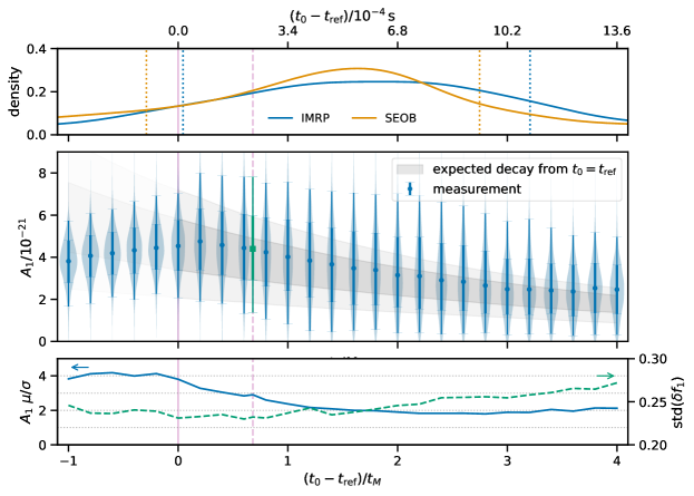
Figure 1: Analysis of the GW150914 ringdown. Top: Posterior for the strain peak time, $\mathrm{max}(h^{2}_{+}+h^{2}_{\times})$, from full IMR analyses with either IMRPhenomPv2 Husa et al. (2016); Khan et al. (2016); Schmidt et al. (2011) (blue) or SEOBNRv4ROM Taracchini et al. (2014); Pürrer (2014, 2016) (orange); dotted lines enclose the 68%-credible symmetric interval. Middle: Posterior for the overtone amplitude $A_{1}$ obtained with a two-tone model ($n=0,1$) applied at different starting times $t_{0}$ (blue, with the preferred start time from Cotesta et al. (2022) in green); the posterior is summarized by the median (circle) and 68% (95%) symmetric credible intervals as thick (thin) vertical lines. The dark (light) gray band shows the 68%-credible (95%-credible) expected decay rate starting from the measurement at $t_{0}=t_{\rm ref}$. Bottom: The left axis shows the ratio of the $A_{1}$ posterior median to the standard deviation (blue solid curve); the right axis shows the standard deviation of the Kerr deviation in the overtone frequency ($\delta f_{1}$), when both $\delta f_{1}$ and $\delta\tau_{1}$ are allowed to vary within $[-0.5,0.5]$. We express time from $t_{\rm ref}$ in seconds (top axis), as well as in units of $t_{M}=GM/c^{3}$ for $M=69M_{\odot}$, i.e., $t_{M}=0.34\,\mathrm{ms}$ (bottom axis). As in Isi et al. (2019), the reference time corresponds to GPS time $t_{\rm ref}=1126259462.423\,\mathrm{s}$ at the LIGO Hanford detector (vertical solid line).

II GW150914 revisited

Here we revisit the GW150914 data to examine the claims in Cotesta et al. (2022), the core of which we understand to be: (1) the chosen analysis start time in Isi et al. (2019) was too early, (2) the detection of the first overtone is unstable against small changes in this start time, and, finally, (3) the overtone amplitude cannot be constrained to be nonzero except significantly before the peak, when the model is known to be invalid.

The reference time in Isi et al. (2019) (a GPS time of $t_{\rm ref}=1126259462.423\,\mathrm{s}$ at the Hanford detector) was taken directly from the original LIGO-Virgo analysis Abbott et al. (2016), where it was claimed to be the peak time; it was chosen before carrying out the analysis and not tuned a posteriori. The actual location of the signal peak is uncertain because it is measured imperfectly from noisy data. It is true that, as pointed out in Cotesta et al. (2022), the reference time in Isi et al. (2019); Abbott et al. (2016) happens to fall before the median of the reconstructed posterior; nevertheless, it lies well within the bulk of the distribution, no more than ${\sim}1\sigma$ away from the median (Fig. 1, top). The choice is thus adequate.

Ringdown analyses are, for the most part, conditional on the chosen truncation time by construction Isi and Farr (2021a). This is because the start time is not a model parameter, but rather defines the data to be analyzed. The meaning and implementation of start-time marginalization are not clear. Techniques like those proposed in Finch and Moore (2021) might offer a possible avenue to allow the start time of the ringdown analysis to vary in a controlled way.

Instead, to account for uncertainty about the arrival time of the peak of the gravitational wave strain, we can always repeat the analysis at different start times. This was the strategy in Cotesta et al. (2022), where it was found that the posterior for the amplitude of the first overtone quickly drops to zero unless the start time is chosen to be significantly before the expected peak, where the quasinormal-mode model is known to be inapplicable. Furthermore, Cotesta et al. (2022) reported a decrease in the overtone amplitude immediately before and after the peak time used in Isi et al. (2019). Altogether, this was interpreted as a sign that the positive identification of the overtone in Isi et al. (2019) was due to a noise artifact. However, we are unable to reproduce any of these observations.

We carry out a similar exercise as in Cotesta et al. (2022) using the publicly available code in Isi and Farr (2021b). The result is summarized in Fig. 1, where the main panel shows the overtone amplitude ($A_{1}$) posterior obtained in a two-tone analysis (i.e., including the $n=0,1$ tones of the $\ell=m=2$ angular harmonic) starting at different times, before and after our previously chosen reference time in Isi et al. (2019) ($t_{0}-t_{\rm ref}=0$ in the plot). The amplitude posterior clearly favors $A_{1}>0$ for a broad range of times, without sharp fluctuations. On the contrary, the posterior decays smoothly in full consistency with the damping expected from the first overtone; this is shown by the gray envelopes, which represent credible regions generated by drawing overtone parameters from the posterior obtained at $t_{0}=t_{\rm ref}$ and projecting the decay forward in time. This result is consistent with the true peak lying close to $t_{\rm ref}$ and the two-tone model being a good fit from that point on.

In Isi et al. (2019) we reported that the $A_{1}$ posterior median fell $3.6\sigma$ away from zero, a measure of overtone detection significance in reference to a model with the fundamental alone, namely, $A_{1}=0$ (but see Isi et al. (2019); Isi and Farr (2021a) for an account of other factors considered, including the effect of allowing for a second overtone). We find a consistent result in our new analysis here, as shown in the bottom panel of Fig. 1 ($\mu/\sigma$, blue solid curve). For $t_{0}>t_{\rm ref}$, this figure of merit decays smoothly, consistent with the evolution of the amplitude posterior.

The bottom panel of Fig. 1 also shows our constraints on deviations from Kerr in the overtone frequency ($\delta f_{1}$) when we allow both the frequency and damping to vary around the Kerr prediction; the constraint is summarized by the $\delta f_{1}$ posterior standard deviation ($\mathrm{std}(\delta f_{1})$, green dashed curve). As we expect, the frequency is best constrained for start times around $t_{\rm ref}$. For later start times, the posterior support for $A_{1}=0$ increases and the frequency is more poorly constrained; this is clear also from the full $\delta f_{1}$ posteriors in Fig. 2. On the other hand, including data significantly before $t_{\rm ref}$ can cause the model to prefer deviations away from the Kerr spectrum, indicating that Kerr quasinormal modes are not a good model for the data at that point—the transition between the two regimes occurs sharply around $t_{0}\approx-1.5t_{M}$ (Fig. 3).

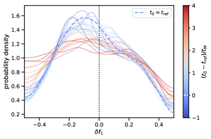
Figure 2: Posterior for deviations from Kerr in the overtone frequency ($\delta f_{1}$) obtained from a two tone analysis in which both $\delta f_{1}$ and $\delta\tau 1$ are allowed to vary uniformly over $[-0.5,0.5]$. The color of the trace corresponds to the analysis start time. The deviation is implemented such that $f_{1}=f_{1}^{\rm Kerr}\exp(\delta f_{1})$ Isi and Farr (2021a). The result for $t_{0}=t_{\rm ref}$ is highlighted with a dashed trace.

A similar conclusion can be drawn from the posterior for the remnant mass ($M$) and dimensionless spin magnitude ($\chi$) obtained assuming a Kerr spectrum in the analyses of Fig. 1. As shown in Fig. 4, the remnant posterior stabilizes around $t_{0}\approx t_{\rm ref}$, at which point it begins to show better consistency with the expectation from the full inspiral-merger-ringdown analysis (IMR, black dashed). This is not true for a model including the fundamental mode alone (Fig. 5), which fails to agree with the IMR analysis at these early times.

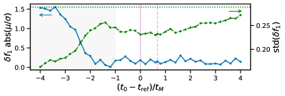
Figure 3: Summary of the posteriors in Fig. 2, plus additional analyses with start times preceding $t_{\rm ref}$ (shaded area). The left axis shows the absolute value of the posterior median-to-standard-deviation ratio for $\delta f_{1}$ (blue solid line); the right axis shows the posterior standard deviation (green dashed line), and the standard deviation of the prior (green dotted line). For $t_{0}\lesssim t_{\rm ref}-2t_{M}$, $\delta f_{1}$ is preferentially negative, indicating lower frequencies are favored.

Besides looking at GW150914 itself, we also inject a number of simulated signals in real data around the event (Fig. 6). We find results consistent with those above: the overtone amplitude posterior varies as might be expected from regular noise fluctuations, and nothing indicates that nonstationarities in the data are derailing the analysis. This experiment is meant to account for non-Gaussianities in actual detector noise; injections in Gaussian noise were already presented in Isi and Farr (2021a).

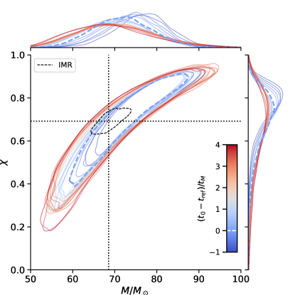
Figure 4: Posterior for the remnant mass ($M$ in solar masses $M_{\odot}$) and dimensionless spin magnitude ($\chi$) obtained with a two-tone analysis ($n=0,1$) beginning at different start times (color). Contours enclose 90% of the probability mass. The result for $t_{0}=t_{\rm ref}$ is highlighted with a dashed blue trace. The result from the IMR analysis is also shown for comparison (dashed black), and was obtained from the LIGO-Virgo samples LIGO Scientific Collaboration and Virgo Collaboration (2018); Abbott et al. (2021c) as detailed in Isi et al. (2019).

Our results here and in Isi et al. (2019), like in any analysis, are predicated on a number of choices about data conditioning and noise power-spectral-density (equivalently, autocovariance-function) estimation. For different reasonable choices for these settings, we obtain slightly different results, but this variation is within expectation and do not alter our conclusions.

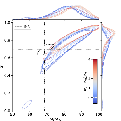
Figure 5: Same as in Fig. 5 but for a model including just the fundamental mode ($n=0$). This model is a poor description of the data at these early times.

III The meaning and implications of detecting a mode

The problem of establishing whether a specific ringdown mode has been detected is made difficult by the fact that the meaning of “detection” is not itself clear in this context. In the regime where we can inarguably expect a superposition of quasinormal modes to be a good description of the data, one can reasonably phrase this question as a choice between $A_{1}=0$ and $A_{1}>0$ within a model including both $n=0,1$—that is, presuming no other quasinormal modes could be expected to be relevant. Already in that simplified scenario the question is technically ill-posed: under that model, the probability that $A_{1}=0$ exactly is effectively zero; this problem appears in other contexts, e.g., the determination of whether a binary black hole system is precessing or whether a given angular harmonic has been detected. The problem is made even murkier if, like in Cotesta et al. (2022), one allows for the possibility that data are not a superposition of damped sinusoids and neither of the $n=0$ nor the $n=0,1$ models are valid. In that case, there is no reason to expect a preference for either model to be informative (whether quantified via the amplitude posterior or a Bayes factor).

Bayes factors are an especially poor tool for this purpose; the drawbacks of Bayes factors in the context of this problem were already discussed in Isi and Farr (2021a), so we do not repeat that here. Nevertheless, Fig. 7 shows the Bayes factors corresponding to the amplitude posteriors in Fig. 1; the Bayes factors favor the presence of the overtone even for $t_{0}>t_{\rm ref}$, unlike in Cotesta et al. (2022). Of course, as remarked in Isi and Farr (2021a), the overall vertical location of the Bayes factor curve can be shifted arbitrarily by modifying the maximum allowed value of $A_{1}$ in the prior (in our case $A_{1}=10^{-20}$). Besdies prior differences, comparing Bayes factors from different analyses can also be inappropriate when the models used are not identical—for that reason comparisons to Bayes factors in Abbott et al. (2021a) are not necessarily interesting or valid.

In any case, the question of whether a mode was detected is inherently “fuzzy.” To quote Gelman and Stern (2006): the difference between statistically significant and not statistically significant is not, itself, statistically significant. This can be seen most clearly in Figure 6, where a signal of constant amplitude injected into noise with (presumably) identical statistical properties generates, on average, a ${\sim}3.5\sigma$ overtone “detection;” but with fluctuations $\sim\pm 1\sigma$, as expected from the intrinsic variation of the particular noise realization from moment to moment. Thus the $3.6\sigma$ “detection” in Isi et al. (2019) could just as easily have been a marginal $2\sigma$ “suggestion” or a $5\sigma$ “confident detection” of the overtone’s presence. Compounded with the above, this makes the question of “how significant is the detection of an overtone” not particularly interesting.

In the end, much of the interest in whether the overtone has positively been detected in GW150914 seems to be fueled by a wish to empirically test the results in Giesler et al. (2019) that the gravitational waves from a binary black hole merger can be described as a superposition of quasinormal modes of the remnant black hole from the peak of the strain onward; however, this urge is misguided. As made clear in Isi et al. (2019), ringdown analyses starting at the peak presume the results of Giesler et al. (2019) to hold, and are not designed to corroborate them (at least not directly).

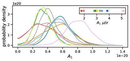
Figure 6: Posterior for the overtone amplitude $A_{1}$ obtained for injections of the GW150914-like numerical simulation SXS:BBH:0305 Kidder et al. (2019); Boyle et al. (2019); Schmidt et al. (2017) into actual LIGO noise around GW150914. We set the total redshifted mass to be $M_{\rm tot}=72\,M_{\odot}$, with a luminosity distance of 450 Mpc. The inset shows the value of the median-to-standard-deviation ratio. The variation in the amplitude posterior agrees with what we expect from Gaussian noise.

As we have argued elsewhere, all that is needed before confronting the data in an analysis like Isi et al. (2019) is the empirical confirmation from numerical relativity studies that, starting from the peak of the strain, the gravitational-wave emission from a binary black hole should be well described by a superposition of quasinormal modes with frequencies and damping rates of the remnant black hole (and not others). This is indeed the conclusion of Giesler et al. (2019) and other studies (particularly Fig. 7 in Giesler et al. (2019)). If, after analyzing real data, the quasinormal modes are not found to be consistent with a final Kerr remnant, then the observation does not agree with what we expect from the merger of two Kerr black holes in general relativity.

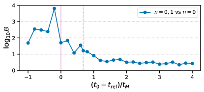
Figure 7: Base-ten logarithm of Bayes factors comparing a two-tone model ($n=0,1$) to a one-tone model ($n=0$) for runs presented in Fig. 1. The values are computed from the amplitude posterior via the Savage-Dickey density ratio, for a prior uniform in $0\leq A_{1}\leq 10^{-20}$.

The ability to carry out such a cross-check is precisely the reason we are interested in identifying multiple quasinormal modes in the first place. To the extent that we can carry out this Kerr-consistency test, the mode was detected. Concretely, as we argued in Isi et al. (2019), the $\delta f_{1}$ (or $\delta\tau_{1}$) posterior can only be informative insofar as the data support a nonzero overtone amplitude. If that is the case, we can say the overtone was “detected” and check for one of two scenarios: (1) the deviation posterior is consistent with zero and thus also with Kerr black holes in general relativity, or (2) the deviation posterior disfavors zero, indicating that one or more of the assumptions in the model is broken (including, potentially, the assumption that general relativity is correct).

IV Conclusion

We have revisited the ringdown of GW150914 finding our previous claims in Isi et al. (2019) to be robust against choices in analysis start time, within the expected location of the signal peak from inspiral-merger-ringdown analyses. We cannot reproduce the claims to the contrary presented in Cotesta et al. (2022). The robustness of our observations against choices of sampling rate and power-spectrum estimation methods gives us additional confidence in our results. We make code to reproduce results in this paper available in Isi and Farr (2022).