Learning fair representation with a parametric integral probability metric

Abstract

As they have a vital effect on social decision-making, AI algorithms should be not only accurate but also fair. Among various algorithms for fairness AI, learning fair representation (LFR), whose goal is to find a fair representation with respect to sensitive variables such as gender and race, has received much attention. For LFR, the adversarial training scheme is popularly employed as is done in the generative adversarial network type algorithms. The choice of a discriminator, however, is done heuristically without justification. In this paper, we propose a new adversarial training scheme for LFR, where the integral probability metric (IPM) with a specific parametric family of discriminators is used. The most notable result of the proposed LFR algorithm is its theoretical guarantee about the fairness of the final prediction model, which has not been considered yet. That is, we derive theoretical relations between the fairness of representation and the fairness of the prediction model built on the top of the representation (i.e., using the representation as the input). Moreover, by numerical experiments, we show that our proposed LFR algorithm is computationally lighter and more stable, and the final prediction model is competitive or superior to other LFR algorithms using more complex discriminators.

1 Introduction

Artificial intelligence (AI) has accomplished tremendous success in various real-world domains. The key of success of AI is “learning from data”. However, in many cases, data include historical bias against certain socially sensitive groups such as gender, race, religion, etc (Feldman et al., 2015; Angwin et al., 2016; Kleinberg et al., 2018; Mehrabi et al., 2019), and trained AI models from such biased data could also impose bias or unfairness against sensitive groups. As AI has a wide range of influences on human social life, issues of transparency and ethics of AI are emerging. Therefore, designing an AI algorithm which is accurate and fair simultaneously has become a crucial research topic (Calders et al., 2009; Feldman et al., 2015; Barocas & Selbst, 2016; Hardt et al., 2016; Zafar et al., 2017; Donini et al., 2018; Agarwal et al., 2018; Quadrianto et al., 2019b).

Among various researches related to fair AI, learning fair representation (LFR) has received much attention recently (Zemel et al., 2013; Xu et al., 2018; Quadrianto et al., 2019a; Ruoss et al., 2020; Gitiaux & Rangwala, 2021; Zeng et al., 2021). Fair representation typically means a feature vector obtained by transforming the data such that the distributions of the feature vector for each sensitive group are similar. Once the fair representation is learned, any prediction models constructed on the top of the fair representation (i.e. using the representation as an input vector) are expected to be fair (Zemel et al., 2013; Madras et al., 2018).

A popular approach for LFR is to use the adversarial training scheme (Edwards & Storkey, 2016; Madras et al., 2018). As is done in the generative adversarial network (GAN, Goodfellow et al. (2014)), the algorithm seeks a representation that fools the discriminator the best that tries to predict which sensitive group a given representation belongs. Different algorithms to learn the discriminator result in different algorithms for LFR.

Despite their considerable success, there are still theoretical and practical limitations in the existing learning algorithms for fair representation based on the adversarial training scheme. First of all, it is not clear how the level of fairness of the representation affects the level of fairness of the final prediction model (built on the top of the representation). This problem is important since the final goal of LFR is to construct fair prediction models.

In this paper, we consider the adversarial training scheme based on the integral probability metric (IPM). The IPM, which includes the Wasserstein distance (Kantorovich & Rubinstein, 1958; Villani, 2008) as a special case, has been widely used for learning generative models (e.g. Wasserstein GAN, Arjovsky et al. (2017)), but has not been used for fair representation. An advantage of using the IPM is that we can control the level of fairness of the final prediction model by controlling the level of fairness of the representation relatively easily.

The second problem we study, which is the main contribution of this paper, is the choice of the class of discriminators. Deep neural networks (DNNs) are popularly used for the discriminator (Goodfellow et al., 2014; Arjovsky et al., 2017; Madras et al., 2018; Creager et al., 2019; Ansari et al., 2020), but the choice of the architecture (the numbers of layers and nodes at each layer) is decided rather heuristically without justification. In this paper, we propose a specific parametric family of discriminators and provide theoretical guarantees of the fairness of the final prediction models in terms of the fairness of the representation for large classes of prediction models.

By applying the IPM with the proposed parametric family of discriminators, we propose a new learning algorithm for fair representation abbreviated by the sIPM-LFR (sigmoid IPM for Learning Fair Representation). Along with the theoretical guarantees, the sIPM-LFR has several advantages over existing LFR algorithms. For example, the sIPM-LFR is computationally lighter, more stable, and less prone to bad local minima. Moreover, the final prediction model is competitive or superior in prediction performance to those from other LFR algorithms.

This paper is organized as follows. In Section 2, we review related studies about fairness of AI. The sIPM-LFR algorithm is proposed in Section 3, and the results of theoretical studies are presented in Section 4. Numerical studies are conducted in Section 5 and concluding remarks follow in Section 6.

The main contributions of this work are summarized as follows.

• We propose a simple but powerful fair representation learning method by developing a new adversarial training scheme based on a parametric IPM.

• We give theoretical guarantees about fairness of the final prediction model in terms of fairness of the representation.

• We empirically show that our algorithm is competitive or even superior to other existing LFR algorithms.

2 Related works

Algorithmic fairness

Generally, various concepts of fair prediction models can be summarized into three categories. The first category is group fairness which requires that certain statistics of the prediction model at each sensitive group are similar (Calders et al., 2009; Barocas & Selbst, 2016).

The second notion of fair prediction models is individual fairness, which aims at treating similar inputs similarly (Dwork et al., 2012) regardless of sensitive groups. Various practical algorithms and their theoretical properties have been proposed and studied by Yona & Rothblum (2018); Sharifi-Malvajerdi et al. (2019); Mukherjee et al. (2020a, b).

The third concept of fair prediction models is counterfactual fairness (Kusner et al., 2017), which can be considered as a compromise between group fairness and individual fairness. Simply speaking, counterfactual fairness requires that similar individuals only from different sensitive groups should have similar prediction values. The notion of counterfactual is used to define similar individuals from different sensitive groups (Wu et al., 2019b; Chiappa, 2019; Garg et al., 2019).

Learning fair representations

LFR has a different strategy than the fair AI algorithms mentioned in the previous subsection. Instead of constructing fair prediction models directly, LFR first constructs a fair representation such that the distributions of the representation for each sensitive group are similar. Then, LFR learns a prediction model on the top of the representation (i.e. using the fair representation as an input). LFR has been initially considered by Zemel et al. (2013), and many advanced algorithms have been developed (Xu et al., 2018; Creager et al., 2019; Quadrianto et al., 2019a; Ruoss et al., 2020; Gitiaux & Rangwala, 2021; Zeng et al., 2021) afterward.

One of the most pivotal learning frameworks of LFR is the adversarial training scheme (Edwards & Storkey, 2016; Madras et al., 2018). Those algorithms try to fool a given discriminator similar to that of GAN does (Goodfellow et al., 2014). The aim of this paper is to propose a new adversarial training scheme for LFR which is computationally easier and has desirable theoretical guarantees.

3 Learning fair representation by use of a parametric IPM

In this section, we propose a new learning algorithm for fair representation. In particular, we develop a parametric IPM to measure the fairness of a given representation mapping. We first review the population version of the existing learning algorithms for fair representation and explain problems when we modify the population version to the sample version and propose a parametric IPM to resolve the problems.

3.1 Notations and Preliminaries

Notations

Let $\mathbf{X}\in\mathcal{X}\subset\mathbb{R}^{d}$, $S\in\{0,1\}$, and $Y\in\{0,1\}$ be the non-sensitive random input vector, (binary) sensitive random input variable and (binary) output variable whose joint distribution is $\mathbb{P}.$ Also let $\mathbf{Z}:=h(\mathbf{X},S)$ be the representation of an input vector $(\bm{X},S)$ obtained by an encoding function $h:{\cal X}\times\{0,1\}\to{\cal Z}\subset\mathbb{R}^{m}$. Note that we allow the encoding function depending on both non-sensitive and sensitive inputs as Madras et al. (2018) did. Let $f:{\cal Z}\to\mathbb{R}$ and $f_{D}:{\cal Z}\to{\cal X}\times\{0,1\}$ be a prediction model and a decoding function, respectively. For technical simplicity, we assume that ${\cal Z}$ is bounded and $\sup_{{\bf z}\in{\cal Z}}|f({\bf z})|\leq F$ for some constant $F>0.$

Fairness for DP

Fair representation is closely related to demographic parity (DP) which is a concept for group fairness. In fact, we will see later that the prediction model $f\circ h$ can be fair in view of DP when the representation $\mathbf{Z}$ is fair in a certain sense. Here, we briefly review the notion of fairness for DP.

Let $\phi$ be a function from $\mathbb{R}$ to $\mathbb{R}.$ For a given prediction model $g:{\cal X}\times\{0,1\}\rightarrow\mathbb{R},$ we say that the level of $\phi$-fairness of $g$ is $\epsilon$ if $DP_{\phi}(g)<\epsilon,$ where

$$DP_{\phi}(g)=|\mathbb{E}(\phi\circ g(\bm{X},S)|S=0)-\mathbb{E}(\phi\circ g(\bm{X},S)|S=1)|.$$ (1)

Various definitions of DP-fairness are special cases of the $\phi$-fairness. The original DP-fairness uses $\phi(w)=\mathbb{I}(w\geq 0)$ (Calders et al., 2009; Barocas & Selbst, 2016), and $\phi(w)=(w+1)_{+}$ is popularly used as a convex surrogate of $\mathbb{I}(w\geq 0)$ (Wu et al., 2019a; Lohaus et al., 2020). When $\phi(w)=w,$ the corresponding fairness measure becomes the mean DP (MDP, Madras et al. (2018); Chuang & Mroueh (2021)).

3.2 Description of LFR algorithms

The goal of LFR is to find an encoding function $h$ such that

$$\mathbb{P}\left\{h(\bm{X},S)\in\cdot|S=0\right\}\approx\mathbb{P}\left\{h(\bm{X},S)\in\cdot|S=1\right\}.$$ (2)

Once we have the encoding function, we construct a prediction model on the representation space ${\cal Z}.$ That is, the final prediction model $g$ is given as $g(\bm{x},s)=f\circ h(\bm{x},s),$ where $f$ is a prediction model from ${\cal Z}$ to $\mathbb{R}.$ Due to (2), we expect that

$$\mathbb{P}\left\{g(\bm{X},S)\in\cdot|S=0\right\}\approx\mathbb{P}\left\{g(\bm{X},S)\in\cdot|S=1\right\}.$$

and thus the prediction model is expected to be DP-fair.

The basic algorithm of LFR consists of the following two steps. The first step is to choose a deviance measure $d$ between two distributions and a class ${\cal H}$ of encoding functions and the second step is to find an encoding function $h$ which minimizes $d(\mathbb{P}_{0}^{h},\mathbb{P}_{1}^{h}),$ where $\mathbb{P}_{s}^{h}$ is the conditional distribution of $h(\bm{X},S)$ given $S=s$ for $s\in\{0,1\}.$

In turn, to define a deviance measure, the adversarial training scheme is popularly employed. For a given class of discriminators ${\cal V}$ and a given classification loss $l,$ one possible deviance measure is defined as $d(\mathbb{P}_{0}^{h},\mathbb{P}_{1}^{h})=\sup_{v\in{\cal V}}\mathbb{E}\left\{l(S,v\circ h(\bm{X},S)\right\}.$ Various classification losses have been used for learning fair representation: Edwards & Storkey (2016) uses the cross-entropy loss and Madras et al. (2018) uses the $L_{1}$ loss.

The minimizer of $d(\mathbb{P}_{0}^{h},\mathbb{P}_{1}^{h}),$ however, is not unique in most cases. For example, if there exists $h$ such that $d(\mathbb{P}_{0}^{h},\mathbb{P}_{1}^{h})=0,$ then any encoding function given as $\xi\circ h$ for any $\xi:{\cal Z}\rightarrow{\cal Z}$ also has the zero deviance. Also, an encoder derived as such might not provide helpful information (e.g., $h(\cdot)=0$).

There are two ways to resolve these problems in the adversarial training scheme for LFR - supervised and unsupervised methods. For the supervised adversarial training scheme, we choose a set ${\cal F}$ of prediction models on ${\cal Z}$ and then learn $h$ as well as $f$ by minimizing

$$L(f\circ h)+\lambda d(\mathbb{P}_{0}^{h},\mathbb{P}_{1}^{h})$$ (3)

in $f\in{\cal F}$ and $h\in{\cal H},$ where $L$ is a certain classification risk for $Y$ such as the cross-entropy and $\lambda>0$ is a regularization parameter.

For the unsupervised adversarial training scheme, we first choose a set ${\cal F}_{D}$ of decoding functions from ${\cal Z}$ to ${\cal X}\times\{0,1\},$ then we learn the encoding function by minimizing

$$L_{recon}(f_{D}\circ h)+\lambda d(\mathbb{P}_{0}^{h},\mathbb{P}_{1}^{h}),$$ (4)

where $L_{recon}$ is a reconstruction error. When the learning procedure of $h$ finishes, the extracted fair representation are used to solve various downstream classification tasks. That is, we do not use the label information $Y$ when we learn $h,$ which is an advantage of the unsupervised adversarial training scheme.

When we do not know the population distribution $\mathbb{P}$ but we have data, a standard method of LFR is to replace $\mathbb{P}$ by its empirical counterpart $\mathbb{P}_{n}(\cdot)=\sum_{i=1}^{n}\delta_{({\bf x}_{i},y_{i},s_{i})}(\cdot)/n,$ the empirical distribution, where $\delta_{a}$ is the Dirac-delta function and $\{({\bf x}_{i},y_{i},s_{i})\}_{i=1}^{n}$ is a given training dataset.

Regarding optimizing the formulas (3) and (4) in practice, obtaining the value of $d(\mathbb{P}_{0}^{h},\mathbb{P}_{1}^{h})$ is time-consuming since we have to find a discriminator maximizing the classification loss of $S$ (i.e. $\sup_{v\in{\cal V}}\mathbb{E}\left\{l(S,v\circ h(\bm{X},S)\right\}$). To reduce this computational burden, at each update, we apply a gradient ascent algorithm to update the parameters in the discriminator few times, e.g. five times, as is done by Goodfellow et al. (2014).

The aim of this paper is to propose a novel measure for $d(\mathbb{P}_{0}^{h},\mathbb{P}_{1}^{h})$ used in (3) and (4), which we will describe in the subsequent sections. For details of the corresponding learning algorithm, see Section B.3.

3.3 Learning fair representation with IPM

In this paper, we consider the integral probability metric (IPM) as the deviance measure for LFR. For a given class ${\cal V}$ of discriminators from ${\cal Z}$ to $\mathbb{R},$ the IPM $d_{{\cal V}}(\mathbb{P}_{0},\mathbb{P}_{1})$ for given two probability measures $\mathbb{P}_{0}$ and $\mathbb{P}_{1}$ is defined as

$$d_{{\cal V}}(\mathbb{P}_{0},\mathbb{P}_{1})=\sup_{v\in{\cal V}}\left|\int v(\bm{z})(d\mathbb{P}_{0}(\bm{z})-d\mathbb{P}_{1}(\bm{z}))\right|.$$

When ${\cal V}$ includes all Lipschitz functions, then the IPM becomes the well known Wasserstein norm (Kantorovich & Rubinstein, 1958). Even if it is popularly used in various applications of AI including the generative model learning, the IPM has not been studied deeply for LFR.

An obvious advantage of the IPM compared to the other deviance measures is that the level of the IPM is directly related to the level of DP-fairness of the final prediction model. That is, suppose that a given encoding function $h$ satisfies $d_{{\cal V}}(\mathbb{P}_{0}^{h},\mathbb{P}_{1}^{h})<\epsilon,$ then any prediction model given as $f\circ h$ automatically satisfies the level of $\phi$-fairness less $\epsilon,$ as long as $\phi\circ f$ belongs to ${\cal V}.$ For example, suppose that ${\cal V}$ is the set of Lipschitz continuous functions. If $\phi$ is a Lipschitz function with the Lipschitz constant less than or equal to 1, then $\phi\circ f$ belongs to ${\cal V}$ whenever $f\in{\cal V}.$ Examples of $\phi$ with the bounded Lipschitz constant are $\phi(w)=w$ and $\phi(w)=(w+1)_{+}.$

3.4 The sigmoid IPM: A parametric IPM for fair representation

We need to set in advance the function spaces for ${\cal H},{\cal F},$ and ${\cal F}_{D}$ as well as ${\cal V}$ to make the minimization of the regularized empirical risk in (3) or (4) be possible. There are many well known and popularly used models for ${\cal H}$ (e.g. DNN and ConvNet), ${\cal F}$ (e.g. linear, DNN, and Kernel machine (Cortes & Vapnik, 1995)), and ${\cal F}_{D}$ (e.g. DNN and DeConvNet (Noh et al., 2015)). In contrast, the choice of ${\cal V}$ is typically done heuristically. DNNs are popularly used for ${\cal V}$ (Arjovsky et al., 2017), but the choice of the architecture (the numbers of layers and nodes at each layer) is decided without justification. In this subsection, we focus on the choice of ${\cal V}$ and propose a specific parametric family with theoretical justifications in view of DP-fairness.

Suppose that ${\cal H}$ and ${\cal F}$ are given. That is, the final prediction model is given as $f\circ h,$ where $f\in{\cal F}$ and $h\in{\cal H}.$ Also, the fairness function $\phi$ is given. Our mission is to choose ${\cal V}$ such that the level of $\phi$-fairness of the final prediction model can be controlled by controlling the $d_{{\cal V}}(\mathbb{P}_{0}^{h},\mathbb{P}_{1}^{h}).$ This is an important task for the unsupervised LFR since the label $Y$ is not available when fair representation is learned.

To be more specific, we derive a non-decreasing function $\rho:\mathbb{R}_{+}\rightarrow\mathbb{R}_{+}$ such that

$$\sup_{f\in{\cal F}}DP_{\phi}(f\circ h)\leq\rho\left\{d_{{\cal V}}(\mathbb{P}_{0}^{h},\mathbb{P}_{1}^{h})\right\}.$$

That is, we can control the $\phi$-fairness of any $f\circ h$ by controlling the $d_{{\cal V}}$ of $h.$

A naive choice of ${\cal V}$ would be that $\phi\circ f\in{\cal V}$ for all $f\in{\cal F},$ in which case $\rho(\epsilon)=\epsilon.$ Such a choice, however, is not possible for the unsupervised LFR since the prediction model space ${\cal F}$ is selected after learning the fair representation. One may choose a very large ${\cal V}$ so that $\phi\circ{\cal F}\subset{\cal V}$ for most classes of ${\cal F}.$ Such a choice, however, would make the computational cost unnecessarily large and increase the variance of the learned model due to too many parameters in ${\cal V}$ to degrade performance.

We explore an opposite direction: to seek a class of ${\cal V}$ that is small but controls the level of $\phi$-fairness easily. In this paper, we propose a specific parametric family for ${\cal V}$ and show that the $\phi$-fairness of $f\circ h$ can be controlled nicely by $d_{{\cal V}}$ of $h$ for fairly large classes of ${\cal F}.$

In fact, using the parametric IPM is not new. Ansari et al. (2020) considers ${\cal V}_{char}=\{\exp(i\mathbf{t}^{\top}\bm{x}):\mathbf{t}\in\mathbb{R}^{m}\}$ in the GAN algorithm. This class of functions are related to the characteristic function and it is easy to see that $d_{{\cal V}_{char}}(\mathbb{P}_{0},\mathbb{P}_{1})=0$ if and only if $\mathbb{P}_{0}(\cdot)\equiv\mathbb{P}_{1}(\cdot).$ However, it is not clear what happens when $d_{{\cal V}_{char}}(\mathbb{P}_{0},\mathbb{P}_{1})<\epsilon.$ That is, not much is known about which quantities of $\mathbb{P}_{0}$ and $\mathbb{P}_{1}$ are similar. McCullagh (1994) noticed that $d_{{\cal V}_{char}}$ would not be a useful metric between probability measures.

The parametric family we propose in this paper is

$${\cal V}_{sig}=\{\sigma(\theta^{\top}\bm{x}+\mu):\theta\in\mathbb{R}^{m},\mu\in\mathbb{R}\},$$ (5)

where $\sigma(z)=(1+\exp(z))^{-1}$ is the sigmoid function. It is surprising to see that the IPM with this simple ${\cal V}_{sig}$ can control the level of $\phi$-fairness of $f\circ h$ for diverse classes of ${\cal F},$ whose results are rigorously stated in the following section.

Before going further, we give a basic property of the IPM with ${\cal V}_{sig},$ whose proof is stated in Appendix A.

Proposition 3.1.

For two probability measures $\mathbb{P}_{0}$ and $\mathbb{P}_{1},$ $d_{{\cal V}_{sig}}(\mathbb{P}_{0},\mathbb{P}_{1})=0$ if and only if $\mathbb{P}_{0}(\cdot)\equiv\mathbb{P}_{1}(\cdot).$

4 Theoretical studies of the IPM with ${\cal V}_{sig}$

One may concern that the final prediction model $f\circ h$ would not be fair because the class ${\cal V}_{sig}$ of discriminators is too small. In this section, we show that the IPM with ${\cal V}_{sig}$ can control the level of $\phi$-fairness of $f\circ h$ for quite large classes of ${\cal F}$ even if ${\cal V}_{sig}$ is small.

We start with the DP-fairness of the perfectly fair representation, which is a direct corollary of Proposition 3.1. We defer the proofs of all the following theorems to Appendix A.

Theorem 4.1.

If $d_{{\cal V}_{sig}}(\mathbb{P}_{0}^{h},\mathbb{P}_{1}^{h})=0,$ then the $\phi$-fairness of any prediction model $f\circ h$ is always 0.

It is not realizable to get a perfectly fair representation in practice. Instead, we learn an encoding function whose IPM value is close to 0. In the next two subsections, we quantify how small the level of $\phi$-fairness of $f\circ h$ when the $d_{{\cal V}_{sig}}$ of $h$ is small for various classes ${\cal F}$ of $f.$

For technical simplicity, we only consider $\phi$ being a polynomial function (i.e. $\phi(w)=w^{k}$). Note that reasonably smooth functions can be approximated by linear combinations of low order polynomial functions. Hereafter, we denote $\phi_{k}(w)=w^{k}.$

4.1 DP-fairness when ${\cal F}$ is well approximated by a shallow neural network

There is much literature about classes of functions that are well approximated by shallow neural networks with the sigmoid activation function (Barron, 1993; Yukich et al., 1995). In this section, we show that the level of DP-fairness of such functions can be controlled by the level of the sigmoid IPM.

We consider the class ${\cal F}_{a,C}$ of functions considered by Barron (1993); Yukich et al. (1995):

$${\cal F}_{a,C}=\left\{f:\int|\tilde{f}(\bm{w})|d\bm{w}\leq a,\int\|\bm{w}\|_{1}|\tilde{f}(\bm{w})|d\bm{w}\leq C\right\}$$

for positive constants $a$ and $C,$ where $\tilde{f}(\bm{w})=\int e^{-i\bm{w}^{\top}{\bf z}}f({\bf z})d{\bf z}.$

It is known that any function in ${\cal F}_{a,C}$ can be approximated closely by a single-layered shallow neural network with a finite number of hidden nodes (Yukich et al., 1995). Using this proposition, we have the following theorem, whose proof is deferred to Appendix A.

Theorem 4.2.

There exists a constant $c_{k}>0$ such that

$$\sup_{f\in{\cal F}_{a,C}}DP_{\phi_{k}}(f\circ h)\leq{c_{k}}\left\{d_{{\cal V}_{sig}}(\mathbb{P}_{0}^{h},\mathbb{P}_{1}^{h})\right\}^{1/3}.$$ (6)

Theorem 4.2 implies that we can control the level of $\phi$-fairness of the final prediction model $f\circ h$ only by making the $d_{{\cal V}_{sig}}$ of the encoding function $h$ sufficiently small. The exponent term $1/3$ on the right hand side of (6) suggests that a smaller value of $d_{{\cal V}_{sig}}$ of the encoding function $h$ is needed to control the level of $\phi$-fairness of $f.$ This is a price we pay for using a simpler class of discriminators.

The exponent $1/3$ in the right-hand side of (6) may not be tight. We can improve this exponent by assuming more on ${\cal F}_{a,C}.$ The main message of Theorem 4.2 is that the $\phi$-fairness is controlled when shallow neural networks approximate the final prediction model well. However, in the subsequent subsection, we give an interesting example in that the sigmoid IPM amply controls the $\phi$-fairness for a class of functions which is not well approximated by shallow neural networks.

4.2 DP-fairness for $f$ being infinitely differentiable

In general, the encoding function is a complicated mapping (e.g. DNNs) from the input space to the representation space and thus it is reasonable to expect that the prediction model from the representation space to the output is a simple function such as linear models or sufficiently smooth functions (e.g. the reproducing kernel Hilbert space (RKHS) with a smooth kernel). Otherwise, the final prediction model would be overly complicated. For such nice prediction models, we can show that the adversarial training scheme with the sigmoid IPM can control the level of $\phi$-fairness of the final prediction model more tightly.

Let $\mathcal{F}_{\mathcal{C}^{\infty},B}$ be the set of infinite times differentiable functions given as

$$\mathcal{F}_{\mathcal{C}^{\infty},B}=\big{\{} f:{\cal Z}\to\mathbb{R}\ :\ \forall\mathbf{r}\in\mathbb{N}_{0}^{m},$$

$$||D^{\mathbf{r}}f||_{\infty}\leq\sqrt{{\mathbf{r}}!}B^{|\bm{r}|_{1}}\big{\}}$$

for some constant $B>0,$ where $|\bm{r}|_{1}=\sum_{j=1}^{m}r_{j}$ and $D$ is the derivative operator, that is, for a vector ${\bf r}=(r_{1},\cdots,r_{m})$, $D^{{\bf r}}f:=\frac{\partial^{|{\bf r}|_{1}}f}{\partial z_{1}^{r_{1}}\cdots\partial z_{1}^{r_{1}}}.$ The specific bound $\sqrt{{\mathbf{r}}!}B^{|\bm{r}|_{1}}$ for the sup norm of the derivatives is used for $\mathcal{F}_{\mathcal{C}^{\infty},B}$ to include some RKHS with smooth kernels (e.g. radial basis function (RBF) kernel). The following theorem proves that the level of $\phi$-fairness has the same order of the sigmoid IPM for any $f$ in $\mathcal{F}_{\mathcal{C}^{\infty},B}.$

Theorem 4.3.

There exists a constant $c_{k}>0$ such that

$$\sup_{f\in\mathcal{F}_{\mathcal{C}^{\infty},B}}DP_{\phi_{k}}(f\circ h)\leq c_{k}d_{{\cal V}_{sig}}(\mathbb{P}_{0}^{h},\mathbb{P}_{1}^{h}).$$ (7)

Theorem 4.3 indicates that controlling the sigmoid IPM value of the representation $h$ is equivalent to controlling the $\phi$-fairness (up to a constant) of $f\circ h$ whenever $f\in\mathcal{F}_{\mathcal{C}^{\infty},B}.$ This result justifies the sufficiency of the sigmoid IPM for LFR.

Note that the function class ${\cal F}_{{\cal C}^{\infty},B}$ is large enough to include certain function spaces popularly used as the class of prediction models in modern machine learning algorithms. The RKHS with the RBF kernel is such an example, which is stated in the following proposition.

Proposition 4.4.

Let $k_{\gamma}:\mathbb{R}^{m}\times\mathbb{R}^{m}\to\mathbb{R}$ be the RBF kernel with the width $\gamma$ defined as

$$k_{\gamma}({\bf z},{\bf z}^{\prime})=\exp\left(-\frac{\|{\bf z}-{\bf z}^{\prime}\|_{2}^{2}}{\gamma^{2}}\right)$$

and $(\mathcal{H}_{\gamma}({\cal Z}),||\cdot||_{\mathcal{H}_{\gamma}({\cal Z})})$ be the RKHS corresponding to $k_{\gamma}.$ Define ${\cal F}_{k_{\gamma},B}=\{f\in\mathcal{H}_{\gamma}({\cal Z}):||f||_{\mathcal{H}_{\gamma}({\cal Z})}\leq B\}$ for $B>0.$ Then, there exists a $B^{\prime}>0$ such that ${\cal F}_{k_{\gamma},B}\subset{\cal F}_{{\cal C}^{\infty},B^{\prime}}.$

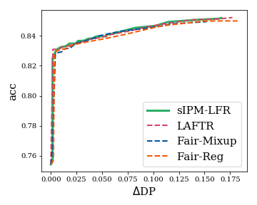
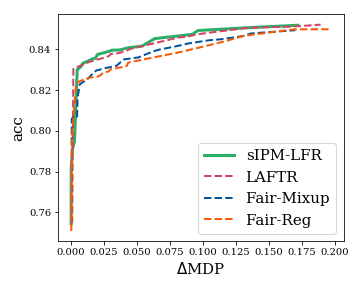
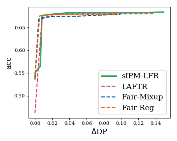
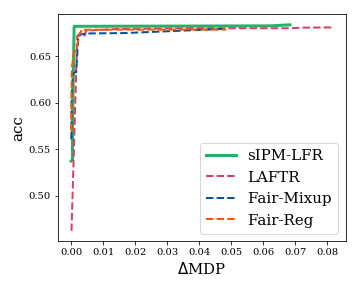
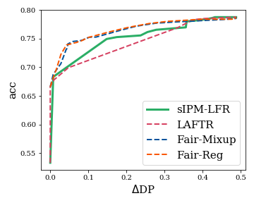
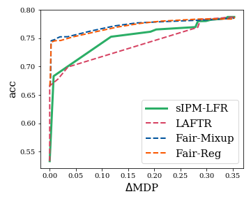
Figure 1: Supervised LFR: Pareto-front lines between the levels of DP-fairness and acc on the test data of (top) Adult, (middle) COMPAS, and (bottom) Health. For the fairness measure, (left) $\Delta\texttt{DP}$ and (right) $\Delta\texttt{MDP}$ are considered.

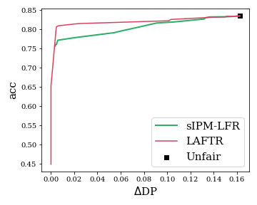
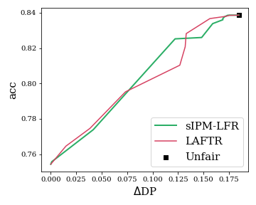
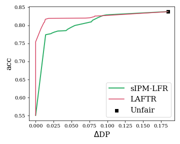
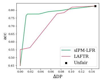
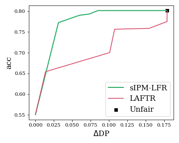
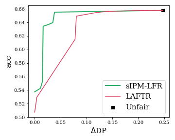
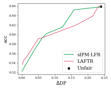
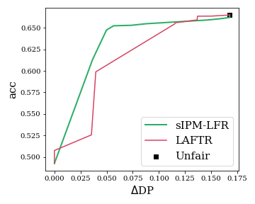
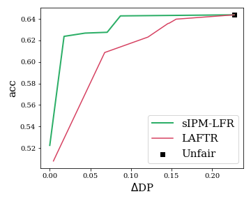
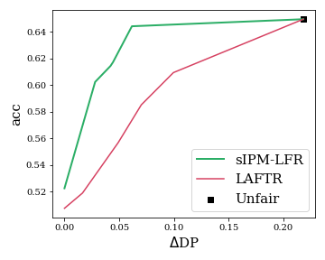
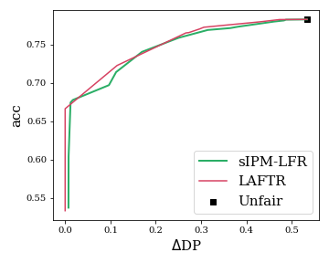
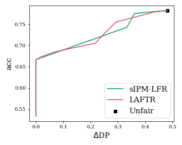
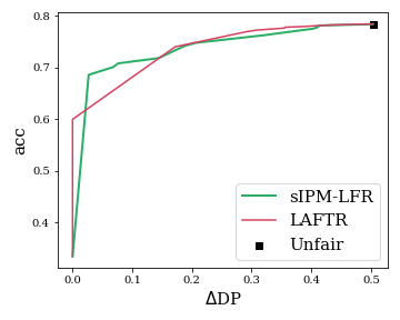
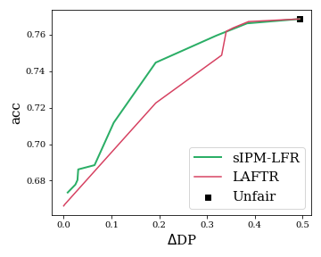
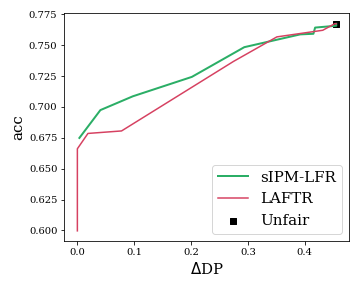
Figure 2: Unsupervised LFR: Pareto-front lines between $\Delta\texttt{DP}$ and acc on the test data of (top) Adult, (middle) COMPAS, and (bottom) Health. The results of the five prediction models are given: (left to right) linear, RBF-SVM, 1-LeakyReLU-NN, 1-Sigmoid-NN, and 2-Sigmoid-NN.

4.3 Extension to other fairness measures

The parametric IPM for DP can be easily extended to other group fairness measures such as the equal opportunity (EOpp) or equalized odds (EO). Let $\mathbb{P}_{s,y}^{h}$ be the distribution of ${\bf Z}|S=s,Y=y$ for $s\in\{0,1\}$ and $y\in\{0,1\}$. For a given function $\phi$ and a prediction function $f$, the fairness levels of EOpp and EO are defined as

$$EOpp_{\phi}(f)=|\mathbb{E}_{Z\sim\mathbb{P}_{0,0}^{h}}[\phi\circ f(Z)]-\mathbb{E}_{Z\sim\mathbb{P}_{1,0}^{h}}[\phi\circ f(Z)]|$$

and

$$EO_{\phi}(f)=\sum_{y\in\{0,1\}}|\mathbb{E}_{Z\sim\mathbb{P}_{0,y}^{h}}[\phi\circ f(Z)]-\mathbb{E}_{Z\sim\mathbb{P}_{1,y}^{h}}[\phi\circ f(Z)]|.$$

Note that the main result of the previous section is to characterize the relationship between $d_{{\cal V}_{sig}}(\mathbb{P}_{0},\mathbb{P}_{1})$ and $|\mathbb{E}_{Z\sim\mathbb{P}_{0}}[\phi\circ f(Z)]-\mathbb{E}_{Z\sim\mathbb{P}_{1}}[\phi\circ f(Z)]|$ for given two distributions $\mathbb{P}_{0}$ and $\mathbb{P}_{1}.$ We can derive similar theoretical results for EOpp and EO simply by letting $\mathbb{P}_{s}$ to $\mathbb{P}_{s,y}^{h}$. If we let $\mathbb{P}_{s}=\mathbb{P}_{s,0}^{h}$, we would obtain the connection between $d_{{\cal V}_{sig}}(\mathbb{P}_{0,0}^{h},\mathbb{P}_{1,0}^{h})$ and $EOpp_{\phi}(f)$. Similarly, we could obtain the connection between $\sum_{y\in\{0,1\}}d_{{\cal V}_{sig}}(\mathbb{P}_{0,y}^{h},\mathbb{P}_{1,y}^{h})$ and $EO_{\phi}(f).$ For learning $f$ and $h$ for EOpp and EO, we minimize (3) and (4) after replacing $d_{{\cal V}_{sig}}(\mathbb{P}_{0}^{h},\mathbb{P}_{1}^{h})$ with $d_{{\cal V}_{sig}}(\mathbb{P}_{0,0}^{h},\mathbb{P}_{1,0}^{h})$ and $\sum_{y\in\{0,1\}}d_{{\cal V}_{sig}}(\mathbb{P}_{0,y}^{h},\mathbb{P}_{1,y}^{h}),$ respectively.

5 Experiments

This section empirically shows that LFR using the sigmoid IPM (sIPM-LFR) performs well by analyzing supervised and unsupervised LFR tasks. Among these two tasks, we focus more on the latter because it is the case where fair representations is more important. We show that the sIPM-LFR yields better and more stable performances than other baselines. For unsupervised LFR, in particular, the representations generated by our method usually give improved prediction accuracies for various downstream tasks.

We also do several ablation studies for the sIPM-LFR algorithm, where the results for the stability issue are reported in the main manuscript, and the others are presented in Appendix E. We here inform that we obtain the results of the baseline algorithms of LFR by our own experiments (i.e. not copied from the related literature) and report the averaged results from five random implementations.

5.1 Experimental setup

Datasets

We analyze three benchmark datasets - 1) Adult (Dua & Graff, 2017), 2) COMPAS , and 3) Health , which are analyzed in Zemel et al. (2013); Edwards & Storkey (2016); Madras et al. (2018); Ruoss et al. (2020) for LFR.

Adult contains personal information of over 40,000 individuals from the 1994 US Census. The label indicates whether each person’s income is over 50K$ or not, and the sensitive variable is gender information.

COMPAS contains criminal information of over 5,000 individuals from Florida. The label is whether each person commits recidivism within two years, and the sensitive variable is race information.

Health contains hospitalization records and insurance claims of over 60,000 patients. The label is the binary Charlson index that estimates the death risk in the future ten years, and the sensitive variable is the binarized age information with a threshold of 70. Health also has tens of auxiliary binary labels, called the primary condition group (PCG) labels, indicating patients’ insurance claim to the specific medical conditions, which can be utilized to conduct further downstream classification tasks. In our experiments, five auxiliary labels that are commonly used in related literature are analyzed.

We split the whole data into training and test data randomly, except for Adult which already consists of training and test data. We split the training data once more into two parts of the ratio 80% and 20%, each of which is used for training and validation, respectively. See Appendix B for more detailed descriptions of the datasets including their pre-processing procedures.

Architectures

We set up the architecture construction scheme similar to other works for LFR (Edwards & Storkey, 2016; Madras et al., 2018). The architecture of the encoder is fixed to a single-layered neural network with the LeakyReLU activation and we consider the value of $m$ as 60, 8, and 40 for Adult, COMPAS, and Health, respectively. Regarding the prediction model $f$, while only single-layered neural network with the LeakyReLU activation (1-LeakyReLU-NN) is used for the supervised LFR, we take four more prediction models into account for unsupervised LFR. That is, we consider five prediction models in total: (i) linear, (ii) SVM with RBF kernel, (iii) 1-LeakyReLU-NN, (iv) 1-Sigmoid-NN, and (v) 2-Sigmoid-NN, where the last two models stand for single-layered and two-layered neural networks with the sigmoid activation, respectively.

Implementation details

We refer to other related studies (Edwards & Storkey, 2016; Madras et al., 2018) for overall implementation options. To solve the supervised LFR, we train the encoder $h$ and classifier $f$ by applying the stochastic gradient descent step to the objective function (3) for 400 training epochs, and the best networks are chosen based on the value of the difference between accuracy and level of DP-fairness, i.e., $\texttt{acc}-\Delta\texttt{DP}$, on validation data.

For the unsupervised LFR, we first minimize the formula (4) to optimize the encoder and decoder for 300 training epochs. From the encoder-decoder pairs obtained at each epoch, we select the best one with the minimum validation loss. Afterward, for given label information $Y,$ we train and select the best downstream classifier by minimizing the standard cross-entropy loss for 100 epochs while freezing the encoder.

Following what Xu et al. (2020) did, for all cases, we apply the Adadelta (Zeiler, 2012) optimizer with a learning rate of 2.0 and a mini-batch size of 512. More detailed descriptions including our pseudo algorithm are in Appendix B.

Evaluation metric

We assess the trade-off between the prediction accuracy (acc) and level of DP-fairness which are summarized by Pareto-front graphs and tables. For the fairness measure, we mainly deal with the original DP denoted by $\Delta\texttt{DP}$ and also consider other variants such as MDP denoted by $\Delta\texttt{MDP}.$ See Appendix C for formulas of the other fairness measures we consider.

Table 1: Unsupervised LFR: acc and $\Delta\texttt{DP}$ for downstream classification tasks on five PCG labels in Health. We use the RBF-SVM for the prediction model.

Target label		Unfair	LAFTR	sIPM-LFR ✓
MSC2A3	acc	0.665	0.642	0.646
	$\Delta\texttt{DP}$	0.110	0.103	0.055
METAB3	acc	0.669	0.662	0.664
	$\Delta\texttt{DP}$	0.093	0.091	0.084
ARTHSPIN	acc	0.695	0.690	0.692
	$\Delta\texttt{DP}$	0.062	0.047	0.036
NEUMENT	acc	0.759	0.730	0.728
	$\Delta\texttt{DP}$	0.302	0.170	0.138
RESPR4	acc	0.730	0.727	0.727
	$\Delta\texttt{DP}$	0.011	0.009	0.003

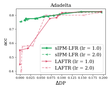
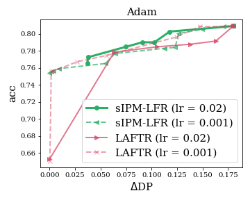
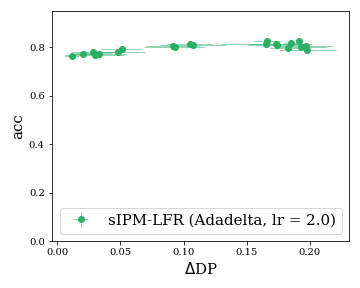
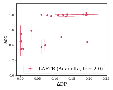
Figure 3: (Upper) Pareto-front lines between $\Delta\texttt{DP}$ and acc with various learning options. (Lower) Scatter plot with standard error bar of $\Delta\texttt{DP}$ and acc with various $\lambda$. Each horizontal and vertical bars present the standard errors for $\Delta\texttt{DP}$ and acc, respectively. All results are from Adult test dataset.

5.2 Supervised learning case

We first evaluate our method in supervised LFR tasks and compare with other baselines including one LFR approach of Madras et al. (2018) (i.e., LAFTR) and two non-LFR approaches in Chuang & Mroueh (2021). Figure 1 presents the Pareto-front trade-off graphs between the level of fairness ($\Delta\texttt{DP}$ and $\Delta\texttt{MDP}$) and acc on each test data. See Appendix D.1 for the results of other fairness measures.

We can clearly see that the proposed sIPM-LFR is compared favorably to the LAFTR even though a much simpler class of discriminators is used. The results amply confirm our theoretical results that the sigmoid IPM is sufficient for learning representations that are fair and good for prediction simultaneously.

It is also interesting to see that the sIPM-LFR is competitive to the two non-LFR algorithms which learn a fair prediction model without learning a representation. That is, the learned fair representation does not lose much information about the label. That is, the sIPM-LFR successively learns a good fair representation.

5.3 Unsupervised learning case

We show that the unsupervised sIPM-LFR provides fair representations of high quality that suit various subsequent downstream supervised tasks. As mentioned in Section 5.1, we first train an encoder by minimizing the objective function (4) without label information of $Y,$ and then train the prediction model with label information while freezing the encoder.

Figure 2 shows the Pareto-front lines between acc and $\Delta\texttt{DP}$ of various prediction models on the three datasets. See Appendix D for the Pareto-front results for other fairness measures.

From the results, we can conclude that the sIPM-LFR is desirable to learn fair representations applicable better to various downstream tasks. In particular, for COMPAS the sIPM-LFR consistently gives superior results with large margins for all of the 5 prediction models. The superiority of the sIPM-LFR regardless of the final prediction model supports our theoretical results that the sigmoid IPM can control the level of fairness well for a large class of prediction models.

We conduct further downstream classification tasks on Health using five auxiliary PCG labels, whose results are summarized in Table 1. We measure the level of DP-fairness while fixing the accuracies at certain levels. It is obvious that the sIPM-LFR consistently achieves lower levels of DP-fairness than the other baselines do, again confirming the superiority of our method.

We also conduct experiments about visualization of the representation distributions and downstream classification with artificial labels. We report the results in Appendix D.

Experiments with additional datasets

Recently, there have been some concerns about the validity of widely-used benchmark datasets in the fair AI domain (Ding et al., 2021; Bao et al., 2021). To answer this concern, we evaluate the sIPM-LFR on two additional datasets: ACSIncome and Toxicity. ACSIncome is a pre-processed version of Adult, and Toxicity is a language dataset containing a large number of Wikipedia comments with ratings of toxicity. For Toxicity, we generate the embedding vectors obtained by the BERT (Devlin et al., 2019) and regard them as input vectors. For the detailed descriptions of those datasets and implementations, see Appendix D.2.

Table 2 shows that for a fixed prediction performance, the sIPM-LFR achieves lower levels of DP-fairness with large margins on the both datasets. We present more results for various $\lambda$ values and various prediction models in Appendix D.2.

Table 2: Unsupervised LFR: acc and $\Delta\texttt{DP}$ for downstream classification tasks on ASSIncome and Toxicity. We use the 1-Sigmoid-NN for the prediction model.

Data (1-Sigmoid-NN)		Unfair	LAFTR	sIPM-LFR ✓
ACSIncome	acc	0.716	0.694	0.695
	$\Delta\texttt{DP}$	0.135	0.027	0.017
Toxicity	acc	0.802	0.790	0.790
	$\Delta\texttt{DP}$	0.042	0.021	0.013

5.4 Stability issue

Compared to other adversarial LFR approaches, the learning procedure of the sIPM-LFR is numerically more stable. We demonstrate this advantage with two additional experiments, whose results are summarized in Figure 3. The two plots at the first row of Figure 3 are the Pareto-front lines of the sIPM-LFR and LAFTR for two optimizers and two learning rates on Adult. It is noticeable that the results of the LAFTR are quite different for different learning rates when the optimizer Adam is used. In contrast, the results of the sIPM-LFR are stable. This stability would be partly because the sIPM-LFR is simpler and thus less vulnerable to bad local minima.

The two plots at the second row are the scatter plots of ($\Delta\texttt{DP}$, acc) for various values of the regularization parameters for Adult. There are many bad solutions observed for the LAFTR while the results for the sIPM-LFR vary smoothly. These results confirm again that the sIPM-LFR is easier to learn good fair representation.

6 Conclusion

In this paper, we devised a simple but powerful LFR method based on the sigmoid IPM called the sIPM-LFR. We proved that the sIPM-LFR can control the level of DP-fairness for a large class of prediction models by controlling the fairness of the representation measured by the proposed parametric IPM. We demonstrated that our learning method is competitive or better than other baselines, especially for unsupervised learning tasks, and is also numerically stable.

We note that any bounded, increasing, and measurable function instead of the sigmoid can be used and similar theoretical results can be derived. We focused on the sigmoid IPM in this paper because the sigmoid is popularly used in machine learning societies.

There are various directions for future works. Theoretically, the level of DP-fairness for diverse classes of functions other than the RKHS with the RBF kernel would be worth pursuing. Also, it would be interesting to investigate other parametric IPMs which have similar properties to the sigmoid IPM.

It would also be interesting to apply the parametric IPM to other AI tasks, such as the generation of tabular data. Unlike image data, it is presumable that tabular data have a relatively smooth distribution. In this case, we conjecture that the parametric IPM would be enough to measure the similarity of two tabular data, which we will pursue in the near future.

Appendix

Appendix A provides the rigorous proofs of theoretical results in Sections 3 and 4. Also, we include an additional theoretical result that the sigmoid IPM can ensure more general types of DP-fairness if the prediction model is simple. The formulas of various fairness measures we consider are listed in Appendix C, and the detailed settings for the experiments are explained in Appendix B. The results of additional experiments are presented in Appendix D.

Appendix A Theoretical proofs

A.1 Proofs of Proposition 3.1, Theorem 4.1, and Theorem 4.2

In this subsection, we let ${\bf Z}_{0}$ and ${\bf Z}_{1}$ are random vectors following the distributions $\mathbbm{P}^{h}_{0}$ and $\mathbbm{P}^{h}_{1}$, respectively. We start with the following lemma which plays a key role in the other proofs.

Lemma A.1.

For any $\epsilon>0$, there exists $c>0$ not depending on $\epsilon$ such that for any two probability measures $\mathbb{P}_{0}$ and $\mathbb{P}_{1}$ defined on $\mathbb{R}^{m}$,

$$d_{\mathcal{V}_{sig}}(\mathbb{P}_{0},\mathbb{P}_{1})<\epsilon$$

implies

$$\sup_{\mathbf{a}\in\mathbb{R}^{m}}\sup_{t\in\mathbb{R}}\left|\mathbbm{P}\left(\mathbf{a}^{\top}\mathbf{U}_{0}\leq t\right)-\mathbbm{P}\left(\mathbf{a}^{\top}\mathbf{U}_{1}\leq t\right)\right|< c\epsilon.$$

where ${\bf U}_{0}$ and ${\bf U}_{1}$ are random vectors following the distributions $\mathbbm{P}_{0}$ and $\mathbbm{P}_{1}$, respectively.

Proof.

Fix $\epsilon>0$ and $\mathbf{a}\in\mathbb{R}^{m}$. We first consider the value of $t\in\mathbb{R}$ that the random variables $\mathbf{a}^{\top}\mathbf{U}_{0}$ and $\mathbf{a}^{\top}\mathbf{U}_{1}$ do not have a point mass at $t.$ Then, there exists a small $\delta$ with $0<\delta<\min(\frac{1}{\log(1/\epsilon)},\frac{1}{\log(1/10)})$ such that

$$\begin{split}\mathbbm{P}\left(\mathbf{a}^{\top}\mathbf{U}_{0}\in[t-\delta,t+\delta]\right)&<\epsilon\\ \mathbbm{P}\left(\mathbf{a}^{\top}\mathbf{U}_{1}\in[t-\delta,t+\delta]\right)&<\epsilon\end{split}$$ (A.1)

hold. By the definition of $d_{\mathcal{V}_{sig}}(\mathbb{P}_{0},\mathbb{P}_{1})<\epsilon$, we have

$$\left|\mathbb{E}\left[\sigma\left(\frac{\mathbf{a}^{\top}\mathbf{U}_{0}-t}{\delta^{2}}\right)\right]-\mathbb{E}\left[\sigma\left(\frac{\mathbf{a}^{\top}\mathbf{U}_{1}-t}{\delta^{2}}\right)\right]\right|<\epsilon.$$ (A.2)

On the other hand, for any $z\in\mathbb{R}$, the following inequality holds:

$$\frac{1}{1+e^{-\frac{1}{\delta}}}\cdot\mathbb{I}\left(z>t+\delta\right)\leq\sigma\left(\frac{z-t}{\delta^{2}}\right)\leq 1-\frac{1}{1+e^{-\frac{1}{\delta}}}\cdot\mathbb{I}\left(z\leq t-\delta\right).$$

Thus for $s=0,1$ we have

$$\frac{1}{1+e^{-\frac{1}{\delta}}}\mathbbm{P}\left(\mathbf{a}^{\top}{\bf U}_{s}>t+\delta\right)\leq\mathbb{E}\left[\sigma\left(\frac{\mathbf{a}^{\top}\mathbf{U}_{s}-t}{\delta^{2}}\right)\right]\leq 1-\frac{1}{1+e^{-\frac{1}{\delta}}}\mathbbm{P}\left(\mathbf{a}^{\top}{\bf U}_{s}\leq t-\delta\right).$$ (A.3)

Also, from (A.1), we can bound the difference of the upper and lower bounds in (A.3):

$$\begin{split}1-\frac{1}{1+e^{-\frac{1}{\delta}}}\left\{\mathbbm{P}\left(\mathbf{a}^{\top}{\bf U}_{s}\leq t-\delta\right)+\mathbbm{P}\left(\mathbf{a}^{\top}{\bf U}_{s}>t+\delta\right)\right\}&\leq 1-\frac{1}{1+e^{-\frac{1}{\delta}}}(1-\epsilon)\\ &\leq 1-\frac{1-\epsilon}{1+\epsilon}\\ &\leq 2\epsilon.\end{split}$$ (A.4)

In turn, from (A.3) and (A.4), we have

$$\left|\mathbb{E}\left[\sigma\left(\frac{\mathbf{a}^{\top}\mathbf{U}_{s}-t}{\delta^{2}}\right)\right]-\left(1-\frac{1}{1+e^{-\frac{1}{\delta}}}\mathbbm{P}\left(\mathbf{a}^{\top}{\bf U}_{s}\leq t-\delta\right)\right)\right|\leq 2\epsilon.$$ (A.5)

Therefore, by (A.1), (A.2), and (A.5), we obtain the following inequality:

$$\begin{split}\frac{1}{1+e^{-\frac{1}{\delta}}}\left|\mathbbm{P}\left(\mathbf{a}^{\top}\mathbf{U}_{0}\leq t\right)-\mathbbm{P}\left(\mathbf{a}^{\top}\mathbf{U}_{1}\leq t\right)\right|&=\left|\left(1-\frac{1}{1+e^{-\frac{1}{\delta}}}\mathbbm{P}\left(\mathbf{a}^{\top}\mathbf{U}_{0}\leq t\right)\right)-\left(1-\frac{1}{1+e^{-\frac{1}{\delta}}}\mathbbm{P}\left(\mathbf{a}^{\top}\mathbf{U}_{1}\leq t\right)\right)\right|\\ &\leq\frac{1}{1+e^{-\frac{1}{\delta}}}\sum_{s\in\{0,1\}}\mathbbm{P}\left(\mathbf{a}^{\top}\mathbf{U}_{s}\in[t-\delta,t]\right)\\ &+\sum_{s\in\{0,1\}}\left|\mathbb{E}\left[\sigma\left(\frac{\mathbf{a}^{\top}\mathbf{U}_{s}-t}{\delta^{2}}\right)\right]-\left(1-\frac{1}{1+e^{-\frac{1}{\delta}}}\mathbbm{P}\left(\mathbf{a}^{\top}{\bf U}_{s}\leq t-\delta\right)\right)\right|\\ &+\left|\mathbb{E}\left[\sigma\left(\frac{\mathbf{a}^{\top}\mathbf{U}_{0}-t}{\delta^{2}}\right)\right]-\mathbb{E}\left[\sigma\left(\frac{\mathbf{a}^{\top}\mathbf{U}_{1}-t}{\delta^{2}}\right)\right]\right|\\ &\leq\frac{2\epsilon}{1+e^{-\frac{1}{\delta}}}+5\epsilon,\end{split}$$

which completes the proof.

For the case where either $\mathbf{a}^{\top}{\bf U}_{0}$ or $\mathbf{a}^{\top}{\bf U}_{1}$ has a point mass at $t$, we can construct a sequence $\{t_{j}\}_{j=1}^{\infty}$ such that 1) $t_{j}\downarrow t$ and 2) neither $\mathbf{a}^{\top}{\bf U}_{0}$ nor $\mathbf{a}^{\top}{\bf U}_{1}$ has a point mass at $\{t_{j}\}_{j=1}^{\infty}$. As $\mathbbm{P}\left(\mathbf{a}^{\top}\mathbf{U}_{s}\leq\cdot\right)$ is right-continuous, the following holds:

$$\lim_{j\to\infty}\left|\mathbbm{P}\left(\mathbf{a}^{\top}\mathbf{U}_{0}\leq t_{j}\right)-\mathbbm{P}\left(\mathbf{a}^{\top}\mathbf{U}_{1}\leq t_{j}\right)\right|=\left|\mathbbm{P}\left(\mathbf{a}^{\top}\mathbf{U}_{0}\leq t\right)-\mathbbm{P}\left(\mathbf{a}^{\top}\mathbf{U}_{1}\leq t\right)\right|<c\epsilon,$$

and the proof is done. $\square$

Proof of Proposition 3.1

Let $\mathbf{U}_{0}$ and $\mathbf{U}_{1}$ are two random vectors whose distributions are $\mathbbm{P}_{0}$ and $\mathbbm{P}_{1}$, respectively.

$(\implies)$ From $d_{\mathcal{V}_{sig}}(\mathbb{P}_{0},\mathbb{P}_{1})=0,$ we have

$$\sup_{\mathbf{a}\in\mathbb{R}^{m}}\sup_{t}\left|\mathbbm{P}\left(\mathbf{a}^{\top}\mathbf{U}_{0}\leq t\right)-\mathbbm{P}\left(\mathbf{a}^{\top}\mathbf{U}_{1}\leq t\right)\right|=0$$

by Lemma A.1. Hence we have $\mathbf{a}^{\top}\mathbf{U}_{0}\overset{d}{=}\mathbf{a}^{\top}\mathbf{U}_{1}$ holds for all $\mathbf{a}\in\mathbb{R}^{m}$, which implies $\mathbb{P}_{0}\equiv\mathbb{P}_{1}$ due to the uniqueness of the characteristic function.

$(\impliedby)$ It is trivial since for any $v\in\mathcal{V}_{sig}$, we have $\int v(\bm{u})(d\mathbbm{P}_{0}(\bm{u})-d\mathbbm{P}_{1}(\bm{u}))=0.$ $\square$

Proof of Theorem 4.1

The proof is trivial by Proposition 3.1.

Proof of Theorem 4.2

Let

$${\cal F}_{n,B}^{NN}=\Big{\{} f({\bf z})=\sum_{k=1}^{n}v_{k}\sigma(\bm{a}_{k}^{\top}{\bf z}+b_{k})+v_{0}:v_{0}\in\mathbb{R},|v_{k}|\leq B,\bm{a}_{k}\in\mathbb{R}^{m},b_{k}\in\mathbb{R},k=1,\ldots,n\Big{\}},$$

for $n\in\mathbb{N}$ and $B>0.$ Since ${\cal Z}$ is bounded, there exists $M>0$ such that ${\cal Z}\subset[-M,M]^{d}$. By Theorem 2.2 of Yukich et al. (1995), for any $f\in{\cal F}_{a,C}$ and $n\in\mathbb{N}$, there exist $\bm{a}_{k}\in\mathbb{R}^{m}$, $b_{k}\in\mathbb{R}$, $|v_{k}|\leq B$ for $k\in\{1,\dots,n\}$ and $v_{0}\in\mathbb{R}$ such that

$$\sup_{{\bf z}\in{\cal Z}}\left|f({\bf z})-\sum_{k=1}^{n}v_{k}\sigma(\bm{a}_{k}^{\top}{\bf z}+b_{k})-v_{0}\right|\leq\frac{C^{\prime}}{\sqrt{n}}$$

for some constant $C^{\prime}>0$. Thus, we have

$$\left|\int\left(f({\bf z})-\sum_{k=1}^{n}v_{k}\sigma(\bm{a}_{k}^{\top}{\bf z}+b_{k})-v_{0}\right)d\mathbb{P}_{0}^{h}({\bf z})\right|\leq \frac{C^{\prime}}{\sqrt{n}}.$$

A similar bound holds for $\mathbb{P}_{1}^{h}.$ Hence, by Proposition 3.1,

$$\left|\int f({\bf z})(d\mathbb{P}_{0}^{h}({\bf z})-d\mathbb{P}_{1}^{h}({\bf z}))\right|\leq \sum_{k=1}^{n}\left|\int(v_{k}\sigma(\bm{a}_{k}^{\top}{\bf z}+b_{k})+v_{0})(d\mathbb{P}_{0}^{h}({\bf z})-d\mathbb{P}_{1}^{h}({\bf z}))\right|+2\frac{C^{\prime}}{\sqrt{n}}$$

$$\leq nBd_{\mathcal{V}_{sig}}(\mathbb{P}_{0}^{h},\mathbb{P}_{1}^{h})+2\frac{C^{\prime}}{\sqrt{n}}$$

$$\leq C^{\prime\prime}d_{\mathcal{V}_{sig}}(\mathbb{P}_{0}^{h},\mathbb{P}_{1}^{h})^{1/3}$$

holds for some constant $C^{\prime\prime}>0$ if we let $n=\lceil\frac{1}{d_{\mathcal{V}_{sig}}(\mathbb{P}_{0}^{h},\mathbb{P}_{1}^{h})^{2/3}}\rceil,$ and thus the proof for $k=1$ is complete with $c_{1}=C^{\prime\prime}$.

For $k>1,$ note that $f^{k}\in{\cal F}_{a^{K},ka^{k-1}C}$ if $f\in{\cal F}_{a,C}$ (see p 940 of (Barron, 1993)) and thus the proof can be done similarly. $\square$

A.2 Proof of Theorem 4.3

To prove Theorem 4.3, we need the following three Lemmas A.2, A.3, and A.4.

Lemma A.2.

For $\forall r_{1},r_{2}\in\mathbb{N}$, let $r:=r_{1}+r_{2}$ and $\lambda_{i}:=-1+\frac{2i}{r}$ for $i=0,1,\dots,r$. Then there exists a vector $(\beta_{0},\beta_{1},\ldots,\beta_{r})\in\mathbb{R}^{r+1}$ such that

$$\sum_{i=0}^{r}\beta_{i}(x+\lambda_{i}y)^{r}=x^{r_{1}}y^{r_{2}}$$ (A.6)

and

$$\sum_{i=0}^{r}|\beta_{i}|<e^{r}$$ (A.7)

for all $x,y\in\mathbb{R}$.

Proof.

We first find a closed form solution of $(\beta_{0},\beta_{1},\ldots,\beta_{r})$ of (A.6) and then show that it satisfies (A.7). Note that if a vector $(\beta_{0},\beta_{1},\dots,\beta_{r})\in\mathbb{R}^{r+1}$ satisfies

$$\sum_{i=0}^{r}\beta_{i}\lambda_{i}^{k} =0\text{ for }k\in\{0,1,\dots,r\}\setminus\{r_{2}\}$$

and

$$\sum_{i=0}^{r}\beta_{i}\lambda_{i}^{r_{2}} =\frac{1}{{r\choose r_{2}}},$$

then it is a solution of (A.6). Let V be the Vandermonde matrix defined as

$$V=\begin{pmatrix}1&1&\dots&1\\ \lambda_{0}&\lambda_{1}&\dots&\lambda_{r}\\ \dots&\dots&\ddots&\dots\\ \lambda_{0}^{r}&\lambda_{1}^{r}&\dots&\lambda_{r}^{r}\end{pmatrix}.$$

Using the Vandermonde matrix, the above two equations can be re-formulated as

$$V\times(\beta_{0},\beta_{1},\dots,\beta_{r})^{\top}=\frac{1}{{r\choose r_{2}}}\bm{e}_{r_{2}+1},$$

where $\bm{e}_{r_{2}+1}\in\mathbb{R}^{r+1}$ is the vector whose $(r_{2}+1)$-th element is 1 and the rests are 0. Then by Man (2017), it is known that $V^{-1}$ can be expressed as the product of two matrices $W$ and $A$, where the matrices $W$ and $A$ are given as

$$W=\left(\begin{array}[]{ccccc}\frac{\lambda_{0}{}^{r}}{\prod_{j\neq 0}\left(\lambda_{0}-\lambda_{j}\right)}&\frac{\lambda_{0}{}^{r-1}}{\prod_{j\neq 0}\left(\lambda_{0}-\lambda_{j}\right)}&\dots&\frac{1}{\prod_{j\neq 0}\left(\lambda_{0}-\lambda_{j}\right)}\\ \frac{\lambda_{1}{}^{r}}{\prod_{j\neq 1}\left(\lambda_{1}-\lambda_{j}\right)}&\frac{\lambda_{1}{}^{r-1}}{\prod_{j\neq 1}\left(\lambda_{1}-\lambda_{j}\right)}&\dots&\frac{1}{\prod_{j\neq 1}\left(\lambda_{1}-\lambda_{j}\right)}\\ \vdots&\vdots&\ddots&\vdots\\ \frac{\lambda_{r}{}^{r}}{\prod_{j\neq r}\left(\lambda_{r}-\lambda_{j}\right)}&\frac{\lambda_{r}{}^{r-1}}{\prod_{j\neq r}\left(\lambda_{r}-\lambda_{j}\right)}&\dots&\frac{1}{\prod_{j\neq r}\left(\lambda_{r}-\lambda_{j}\right)}\end{array}\right)\textup{ and }A=\left(\begin{array}[]{ccccc}a_{0}&0&0&\cdots&0\\ a_{1}&a_{0}&0&\cdots&0\\ a_{2}&a_{1}&a_{0}&\cdots&0\\ \vdots&\vdots&\vdots&\ddots&\vdots\\ a_{r}&a_{r-1}&a_{r-2}&\cdots&a_{0}\end{array}\right),$$

where $a_{0}=1,a_{1}=-\sum\lambda_{j},a_{2}=\sum_{j<l}\lambda_{j}\lambda_{l},a_{3}=-\sum_{j<l<s}\lambda_{j}\lambda_{l}\lambda_{s},\dots,$ and $a_{r+1}=(-1)^{r+1}\prod_{j=0}^{r}\lambda_{j}.$ Since

$$(\beta_{0},\beta_{1},\dots,\beta_{r})^{\top}=\frac{1}{{r\choose r_{2}}}V^{-1}\bm{e}_{r_{2}+1}=\frac{1}{{r\choose r_{2}}}WA\bm{e}_{r_{2}+1}=\frac{1}{{r\choose r_{2}}}W(0,\dots,0,a_{0},a_{1},\dots,a_{r_{1}})^{\top},$$

we obtain the closed form solution $\beta_{i},i=0,1,\ldots,r$ of (A.6) given as

$$\beta_{i}=\frac{1}{{r\choose r_{2}}\prod_{j\neq i}\left(\lambda_{i}-\lambda_{j}\right)}\left(\lambda_{i}^{r_{1}}+\sum_{l=1}^{r_{1}}(-1)^{l}\lambda_{i}^{r_{1}-l}\sum_{k_{1}<\dots<k_{l}}\lambda_{k_{1}}\dots\lambda_{k_{l}}\right).$$ (A.8)

Now we are going to show that the vector $(\beta_{0},\beta_{1},\dots,\beta_{r})$ of (A.8) satisfies (A.7). The numerator of $\beta_{i}$ in (A.8) can be rewritten as

$$\lambda_{i}^{r_{i}}+\sum_{l=1}^{r_{1}}(-1)^{l}\lambda_{i}^{r_{1}-l}\sum_{k_{1}<\dots<k_{l}}\lambda_{k_{1}}\dots\lambda_{k_{l}}= \lambda_{i}^{r_{i}}+\sum_{l=1}^{r_{1}}(-1)^{l}\lambda_{i}^{r_{1}-l}\sum_{\underset{\{k_{1},\dots,k_{l}\}\not\ni i}{k_{1}<\dots<k_{l}}}\lambda_{k_{1}}\dots\lambda_{k_{l}}$$

$$+\sum_{l=1}^{r_{1}}(-1)^{l}\lambda_{i}^{r_{1}-l}\lambda_{i}\sum_{\underset{\{k_{1},\dots,k_{l-1}\}\not\ni i}{k_{1}<\dots<k_{l-1}}}\lambda_{k_{1}}\dots\lambda_{k_{l-1}}$$

$$=\lambda_{i}^{r_{i}}+\sum_{l=1}^{r_{1}}(-1)^{l}\lambda_{i}^{r_{1}-l}\sum_{\underset{\{k_{1},\dots,k_{l}\}\not\ni i}{k_{1}<\dots<k_{l}}}\lambda_{k_{1}}\dots\lambda_{k_{l}}$$

$$-\lambda_{i}^{r_{1}}+(-1)\sum_{l=1}^{r_{1}-1}(-1)^{l}\lambda_{i}^{r_{1}-l}\lambda_{i}\sum_{\underset{\{k_{1},\dots,k_{l}\}\not\ni i}{k_{1}<\dots<k_{l}}}\lambda_{k_{1}}\dots\lambda_{k_{l}}$$

$$=(-1)^{r_{1}}\sum_{\underset{\{k_{1},\dots,k_{{r_{1}}}\}\not\ni i}{k_{1}<\dots<k_{{r_{1}}}}}\lambda_{k_{1}}\dots\lambda_{k_{{r_{1}}}}.$$

Thus, $\beta_{i}$ is given as

$$\beta_{i}=\frac{(-1)^{r_{1}}}{{r\choose r_{2}}}\Big{(}\sum_{\underset{\{k_{1},\dots,k_{{r_{1}}}\}\not\ni i}{k_{1}<\dots<k_{{r_{1}}}}}\lambda_{k_{1}}\dots\lambda_{k_{{r_{1}}}}\Big{)}\Big{/}\Big{(}\prod_{j\neq i}\left(\lambda_{i}-\lambda_{j}\right)\Big{)}.$$

Finally, we can find the lower bound of $|\prod_{j\neq i}\left(\lambda_{i}-\lambda_{j}\right)|$ given as

$$|\prod_{j\neq i}\left(\lambda_{i}-\lambda_{j}\right)| \geq\begin{cases}(\frac{r}{2})!(\frac{r}{2})!/(\frac{r}{2})^{r},&\mbox{if }r\mbox{ is even}\\ (\frac{r+1}{2})!(\frac{r-1}{2})!/(\frac{r}{2})^{r},&\mbox{if }r\mbox{ is odd}\end{cases}$$

$$>(r+1)e^{-r}.$$

The second inequality is derived by the inequality from the Stirling’s approximation, that is,

$$n!>\sqrt{2\pi n}\left(\frac{n}{e}\right)^{n}e^{\frac{1}{12n+1}}>\sqrt{2\pi n}\left(\frac{n}{e}\right)^{n}.$$

Therefore, we finally obtain

$$\sum_{i=0}^{r}|\beta_{i}| <\frac{e^{r}}{(r+1){r\choose r_{2}}}\sum_{i=0}^{r}\sum_{\underset{\{k_{1},\dots,k_{{r_{1}}}\}\not\ni i}{k_{1}<\dots<k_{{r_{1}}}}}|\lambda_{k_{1}}\dots\lambda_{k_{{r_{1}}}}|$$

$$<\frac{e^{r}}{(r+1){r\choose r_{2}}}\sum_{i=0}^{r}\sum_{\underset{\{k_{1},\dots,k_{{r_{1}}}\}\not\ni i}{k_{1}<\dots<k_{{r_{1}}}}}1^{r_{1}}$$

$$=\frac{e^{r}}{(r+1){r\choose r_{2}}}(r+1){r\choose r_{2}}=e^{r},$$

and the proof is done. $\square$

Lemma A.3.

For $\forall u\in\mathbb{N}$ and $\forall r_{1},r_{2},\dots,r_{u}\in\mathbb{N}$, let $r=r_{1}+\dots+r_{u}$. Then there exist a real-valued sequence $\{\beta_{i}\}_{i=0}^{\infty}$ and a 2-dimensional array $\{\lambda_{ij}\}_{i\in\mathbb{N}_{0},j\in\{1,\dots,u\}}$ each of whose elements is bounded by $[-1,1]$ such that

$$\sum_{i}\left[\beta_{i}(\sum_{j=1}^{u}\lambda_{ij}z_{j})^{r}\right]=z_{1}^{r_{1}}z_{2}^{r_{2}}\dots z_{u}^{r_{u}}\textup{ and }\sum_{i}|\beta_{i}|\leq e^{(u-1)r}.$$

holds for all $z_{1},\dots,z_{u}\in\mathbb{R}$.

Proof.

We prove the lemma with the mathematical induction. The statement is obvious for $u=1,$ and we have shown in Lemma A.2 that the statement also holds for $u=2$. Suppose that the statement holds for some $u=N-1\in\mathbb{N}$, and we will prove the statement is also valid when $N$. For given $r_{1},r_{2},\dots,r_{N-1}\in\mathbb{N}$, let $r=r_{1}+\dots+r_{N-1}$. By the assumption, there exist $\beta^{\prime}_{0},\beta^{\prime}_{1},\dots\in\mathbb{R}$ and $\lambda^{\prime}_{ij}\in[-1,1]\text{ for }i\in\mathbb{N}_{0}$ and $j\in\{1,\dots,N-1\}$ such that

$$\sum_{i}\left[\beta^{\prime}_{i}(\sum_{j=1}^{N-1}\lambda^{\prime}_{ij}z_{j})^{r}\right]=z_{1}^{r_{1}}z_{2}^{r_{2}}\dots z_{N-1}^{r_{N-1}}\textup{ and }\sum_{i}|\beta^{\prime}_{i}|<e^{(N-2)r}.$$

Note that by Lemma A.2, for any $r_{N}\in\mathbb{N}$ there exist $\beta^{\prime\prime}_{0},\beta^{\prime\prime}_{1},\dots,\beta^{\prime\prime}_{r+r_{N}}\in\mathbb{R}$ with $\sum_{k=0}^{r+r_{N}}|\beta^{\prime\prime}_{k}|<e^{r+r_{N}}$ and $\lambda^{\prime\prime}_{k}\in[-1,1]$ for $k\in\{0,1,\dots,(r+r_{N})\}$ such that

$$z_{1}^{r_{1}}z_{2}^{r_{2}}\dots z_{N-1}^{r_{N-1}}z_{N}^{r_{N}}= \sum_{i}\left[\beta^{\prime}_{i}(\sum_{j=1}^{N-1}\lambda^{\prime}_{ij}z_{j})^{r}z_{N}^{r_{N}}\right]$$

$$= \sum_{i}\left[\beta^{\prime}_{i}\sum_{k=0}^{r+r_{N}}\left(\beta^{\prime\prime}_{k}(\sum_{j=1}^{N-1}\lambda^{\prime}_{ij}z_{j}+\lambda^{\prime\prime}_{k}z_{N})^{r+r_{N}}\right)\right]$$

$$= \sum_{i}\sum_{k=0}^{r+r_{N}}\left(\beta^{\prime}_{i}\beta^{\prime\prime}_{k}(\sum_{j=1}^{N-1}\lambda^{\prime}_{ij}z_{j}+\lambda^{\prime\prime}_{k}z_{N})^{r+r_{N}}\right).$$

Also, we can check that $\sum_{i}|\sum_{k=0}^{r+r_{N}}\beta^{\prime}_{i}\beta^{\prime\prime}_{k}|<e^{(N-1)(r+r_{N})}$ holds. Thus, the statement holds for $N$ if we set $\beta_{i}=\sum_{k=1}^{r+r_{N}}\beta_{i}^{\prime}\beta_{k}^{\prime\prime},$ for $i\in\mathbb{N}_{0}$ and $\{\lambda_{ij}\}_{i\in\mathbb{N}_{0},j\in\{1,\dots,N\}}$ accordingly. $\square$

Lemma A.4.

Suppose that $d_{{\cal V}_{sig}}(\mathbb{P}_{0}^{h},\mathbb{P}_{1}^{h})<\epsilon$ for a given $\epsilon>0.$ Then for a $m$-dimensional index $\mathbf{r}:=(r_{1},\dots,r_{m})^{\top}\in\mathbb{N}_{0}^{m}$, there exist $c_{1},c_{2}>0$ not depending on $\epsilon$ and $\mathbf{r}$ such that

$$\left|\mathbbm{E}(\mathbf{Z}_{0}^{\mathbf{r}})-\mathbbm{E}(\mathbf{Z}_{1}^{\mathbf{r}})\right|<c_{1}c_{2}^{{|\mathbf{r}|_{1}}}\epsilon$$

holds where ${\bf Z}_{0}$ and ${\bf Z}_{1}$ are random vectors following the distributions $\mathbbm{P}_{0}^{h}$ and $\mathbbm{P}_{1}^{h}$, respectively.

Proof.

Since ${\cal Z}$ is bounded, there exists $M>0$ such that ${\cal Z}\subset[-M,M]^{m}$. By Lemma A.3, there exist a real-valued sequence $\{\beta_{i}\}_{i=0}^{\infty}$ and a 2-dimensional array $\{\lambda_{ij}\}_{i\in\mathbb{N}_{0},j\in\{1,\dots,m\}}$ that each element is bounded by $[-1,1]$ such that

$$\sum_{i}\left[\beta_{i}(\sum_{j=1}^{m}\lambda_{ij}z_{j})^{|\mathbf{r}|_{1}}\right]=z_{1}^{r_{1}}z_{2}^{r_{2}}\dots z_{m}^{r_{m}}\textup{ and }\sum_{i}|\beta_{i}|\leq e^{(m-1)|\mathbf{r}|_{1}}$$

hold for all ${\bf z}\in{\cal Z}$. Thus, we have

$$\left|\mathbbm{E}(\mathbf{Z}_{0}^{\mathbf{r}})-\mathbbm{E}(\mathbf{Z}_{1}^{\mathbf{r}})\right|\leq \sum_{i}|\beta_{i}|\left|\mathbbm{E}\left((\sum_{j=1}^{m}\lambda_{ij}\mathbf{Z}_{0j})^{|\mathbf{r}|_{1}}\right)-\mathbbm{E}\left((\sum_{j=1}^{m}\lambda_{ij}\mathbf{Z}_{1j})^{|\mathbf{r}|_{1}}\right)\right|$$

$$\leq e^{(m-1)|\mathbf{r}|_{1}}\sup_{|\mathbf{a}|_{\infty}\leq 1}\left|\mathbbm{E}\left((\mathbf{a}^{\top}\mathbf{Z}_{0})^{|\mathbf{r}|_{1}}\right)-\mathbbm{E}\left((\mathbf{a}^{\top}\mathbf{Z}_{1})^{|\mathbf{r}|_{1}}\right)\right|.$$

In addition, since the function $s(\cdot):=(\cdot)^{|\mathbf{r}|_{1}}/({|\mathbf{r}|_{1}}(mM)^{{|\mathbf{r}|_{1}}-1})$ is $1$-Lipschitz on $[-mM,mM]$, we have

$$\sup_{|\mathbf{a}|_{\infty}\leq 1}\left|\mathbbm{E}\left((\mathbf{a}^{\top}\mathbf{Z}_{0})^{|\mathbf{r}|_{1}}\right)-\mathbbm{E}\left((\mathbf{a}^{\top}\mathbf{Z}_{1})^{|\mathbf{r}|_{1}}\right)\right| \leq{|\mathbf{r}|_{1}}(mM)^{{|\mathbf{r}|_{1}}-1}\sup_{|\mathbf{a}|_{\infty}\leq 1}\int_{t\in\mathbb{R}}\left|\mathbbm{P}\left(\mathbf{a}^{\top}\mathbf{Z}_{0}\leq t\right)-\mathbbm{P}\left(\mathbf{a}^{\top}\mathbf{Z}_{1}\leq t\right)\right|dt$$

by the property of the Wasserstein metric (Gibbs & Su, 2002). Now, by Lemma A.1, there exist $c_{1},c_{2}>0$ such that

$$\left|\mathbbm{E}(\mathbf{Z}_{0}^{\mathbf{r}})-\mathbbm{E}(\mathbf{Z}_{1}^{\mathbf{r}})\right|\leq c_{1}{c_{2}}^{{|\mathbf{r}|_{1}}}\epsilon,$$

and the proof is done.

$\square$

Proof of Theorem 4.3

By using Taylor’s expansion, we can write

$$\begin{split}\phi_{k}(f(\mathbf{z}))=f(\mathbf{z})^{k}=\sum_{\bm{j}\in\mathbb{N}_{0}^{m}}\frac{a_{\bm{j},k}}{\bm{j}!}\mathbf{z}^{\bm{j}},\end{split}$$

where $\bm{j}=(j_{1},\dots,j_{m})\in\mathbb{N}_{0}^{m}$ and $a_{\bm{j},k}=D^{\bm{j}}(f^{k})|_{{\bf z}=0}.$ For a given $\bm{j},$ we are going to inductively show that

$$\begin{split}|a_{\bm{j},k}|\leq\sqrt{\bm{j}!}(kB)^{|\bm{j}|_{1}}\end{split}$$ (A.9)

for all $k\in\mathbb{N}.$ The case when $k=1$ is trivial due to the definition of $\mathcal{F}_{{\cal C}^{\infty},B}.$ Suppose the equation (A.9) holds when $k=N-1\geq 1$ for some $N.$ Then, for $k=N,$

$$f(\mathbf{z})^{N}=f(\mathbf{z})^{N-1}f(\mathbf{z})=\left(\sum_{\bm{l}\in\mathbb{N}_{0}^{m}}\frac{a_{\bm{l},N-1}}{\bm{l}!}\mathbf{z}^{\bm{l}}\right)\left(\sum_{\bm{m}\in\mathbb{N}_{0}^{m}}\frac{a_{\bm{m},1}}{\bm{m}!}\mathbf{z}^{\bm{m}}\right).$$

Thus, the absolute value of the $\mathbf{z}^{\bm{j}}$’s coefficient for $f(\mathbf{z})^{N}$ satisfies

$$\left|\sum_{\bm{h}\in\mathbb{N}_{0}^{m},\bm{h}\leq\bm{j}}\frac{a_{\bm{h},k-1}}{\bm{h}!}\frac{a_{\bm{j}-\bm{h},1}}{(\bm{j}-\bm{h})!}\right|\leq \sum_{\bm{h}\in\mathbb{N}_{0}^{m},\bm{h}\leq\bm{j}}\frac{\sqrt{\bm{h}!}((k-1)B)^{|\bm{h}|_{1}}}{\bm{h}!}\frac{\sqrt{\bm{(j-h)}!}B^{|\bm{j}-\bm{h}|_{1}}}{(\bm{j}-\bm{h})!}$$

$$= \frac{B^{|\bm{j}|_{1}}}{\sqrt{\bm{j}!}}\sum_{h_{1}=0}^{j_{1}}\dots\sum_{h_{m}=0}^{j_{m}}\left(\sqrt{{j_{1}\choose h_{1}}}(k-1)^{h_{1}}\right)\cdots\left(\sqrt{{j_{m}\choose h_{m}}}(k-1)^{h_{m}}\right)$$

$$= \frac{B^{|\bm{j}|_{1}}}{\sqrt{\bm{j}!}}\left(\sum_{h_{1}=0}^{j_{1}}\sqrt{{j_{1}\choose h_{1}}}(k-1)^{h_{1}}\right)\cdots\left(\sum_{h_{m}=0}^{j_{m}}\sqrt{{j_{m}\choose h_{m}}}(k-1)^{h_{m}}\right)$$

$$\leq \frac{B^{|\bm{j}|_{1}}}{\sqrt{\bm{j}!}}\left(\sum_{h_{1}=0}^{j_{1}}{j_{1}\choose h_{1}}(k-1)^{h_{1}}\right)\cdots\left(\sum_{h_{m}=0}^{j_{m}}{j_{m}\choose h_{m}}(k-1)^{h_{m}}\right)$$

$$= \frac{\sqrt{\bm{j}!}(kB)^{|\bm{j}|_{1}}}{\bm{j}!},$$

which implies that (A.9) holds for all $\bm{j}\in\mathbb{N}_{0}^{m}$ and $k\in\mathbb{N}$. Thus, we have

$$\begin{split}\left|\int f(\mathbf{z})^{k}(d\mathbb{P}_{0}^{h}({\bf z})-d\mathbb{P}_{1}^{h}({\bf z}))\right|\leq&\sum_{\bm{j}\in\mathbb{N}_{0}^{m}}\left|\frac{a_{\bm{j},k}}{\bm{j}!}\right|\left|\int\mathbf{z}^{\bm{j}}(d\mathbb{P}_{0}^{h}({\bf z})-d\mathbb{P}_{1}^{h}({\bf z}))\right|\\ \leq&C_{2}d_{{\cal V}_{sig}}(\mathbb{P}_{0}^{h},\mathbb{P}_{1}^{h})\sum_{\bm{j}\in\mathbb{N}_{0}^{m}}\left|\frac{(C_{1}kB)^{|\bm{j}|_{1}}}{\sqrt{\bm{j}!}}\right|\\ \leq&C_{2}2^{m}\max(1,C_{1}kB)d_{{\cal V}_{sig}}(\mathbb{P}_{0}^{h},\mathbb{P}_{1}^{h})\sum_{\bm{j}\in\mathbb{N}_{0}^{m}}\left|\frac{(C_{1}kB)^{2|\bm{j}|_{1}}}{\bm{j}!}\right|\\ =&C_{2}2^{m}\max(1,C_{1}kB)d_{{\cal V}_{sig}}(\mathbb{P}_{0}^{h},\mathbb{P}_{1}^{h})\exp((C_{1}kB)^{2})\end{split}$$

for some $C_{1}$, $C_{2}>0,$ where the second and third inequalities are due to Lemma A.4 and $\sqrt{\bm{j}!}>(\lfloor\bm{j}/2\rfloor)!,$ respectively, which completes the proof. $\square$

A.3 Proof of Proposition 4.4

Proof of Proposition 4.4

The proof is a slight modification of the proof of Theorem 4.48 in Steinwart & Christmann (2008). Let $V_{\gamma}:L_{2}({\cal Z})\to\mathcal{H}_{\gamma}({\cal Z})$ be the metric surjection defined by

$$V_{\gamma}g(\bm{z})=\frac{2^{m/2}}{\gamma^{m/2}\pi^{m/4}}\int_{\mathbb{R}^{m}}e^{-2\gamma^{-2}\|\bm{z}-\bm{y}\|_{2}^{2}}g(\bm{y})d\bm{y}$$

for $g\in L_{2}\left(\mathbb{R}^{m}\right)$ and $\bm{z}\in{\cal Z}.$ Then for a fixed $f\in\mathcal{H}_{\gamma}({\cal Z})$, there exists a $g\in L_{2}\left(\mathbb{R}^{m}\right)$ such that $V_{\gamma}g=f$ and $\|g\|_{L_{2}\left(\mathbb{R}^{m}\right)}\leq 2\|f\|_{\mathcal{H}_{\gamma}({\cal Z})}$.

For $\bm{r}\in\mathbb{N}_{0}^{m}$ and $\bm{z}\in{\cal Z}$, we have

$$|D^{\mathbf{r}}f(\bm{z})|= \frac{2^{m/2}}{\gamma^{m/2}\pi^{m/4}}\left|D^{\mathbf{r}}\int_{\mathbb{R}^{m}}e^{-2\gamma^{-2}\|\bm{z}-\bm{y}\|_{2}^{2}}g(\bm{y})d\bm{y}\right|$$

$$\leq \frac{2^{m/2}}{\gamma^{m/2}\pi^{m/4}}\int_{\mathbb{R}^{m}}\left|D^{\mathbf{r}}e^{-2\gamma^{-2}\|\bm{z}-\bm{y}\|_{2}^{2}}g(\bm{y})\right|d\bm{y}$$

$$\leq \frac{2^{m/2}}{\gamma^{m/2}\pi^{m/4}}\|g\|_{L_{2}\left(\mathbb{R}^{m}\right)}\sqrt{\int_{\mathbb{R}^{m}}\left(D^{\mathbf{r}}e^{-2\gamma^{-2}\|\bm{z}-\bm{y}\|_{2}^{2}}\right)^{2}d\bm{y}},$$ (A.10)

where the last inequality holds by Hölder’s inequality.

Now, recall that for $r\in\mathbb{N}_{0}$, the $r$-th Hermite polynomial is defined by

$$h_{r}(t)=(-1)^{r}e^{t^{2}}\frac{d^{r}}{dt^{r}}e^{-t^{2}},t\in\mathbb{R},$$ (A.11)

which has the following property

$$\int_{-\infty}^{\infty}h_{r_{1}}(t)h_{r_{2}}(t)e^{-t^{2}}dt=2^{r_{1}}{r_{1}}!\sqrt{\pi}\delta_{r_{1},r_{2}},$$ (A.12)

where $\delta_{r_{1},r_{2}}:=\mathbb{I}(r_{1}=r_{2})$ is the Kronecker symbol. By (A.11), we have

$$\frac{d^{r}}{dt^{r}}e^{-2\gamma^{-2}(t-s)^{2}}=\left(-\sqrt{2}\gamma^{-1}\right)^{r}e^{-2\gamma^{-2}(t-s)^{2}}h_{r}\left(\sqrt{2}\gamma^{-1}(t-s)\right)$$

and hence

$$\int_{\mathbb{R}}\left|\frac{d^{r}}{dt^{r}}e^{-2\gamma^{-2}(t-s)^{2}}\right|^{2}ds= \left(2\gamma^{-2}\right)^{r}\int_{\mathbb{R}}e^{-4\gamma^{-2}(t-s)^{2}}h_{r}^{2}\left(\sqrt{2}\gamma^{-1}(t-s)\right)ds$$

$$= \left(2\gamma^{-2}\right)^{r}\int_{\mathbb{R}}e^{-4\gamma^{-2}s^{2}}h_{r}^{2}\left(\sqrt{2}\gamma^{-1}s\right)ds$$

$$= \left(\sqrt{2}\gamma^{-1}\right)^{2r-1}\int_{\mathbb{R}}e^{-2s^{2}}h_{r}^{2}(s)ds$$

$$\leq \sqrt{\pi}2^{2r-1/2}r!\gamma^{1-2r},$$ (A.13)

where the last inequality holds by (A.12).

Since $e^{-2\gamma^{-2}\|\bm{z}-\bm{y}\|_{2}^{2}}=\prod_{i=1}^{m}e^{-2\gamma^{-2}\left(z_{i}-y_{i}\right)^{2}}$ holds, (A.10) and (A.13) imply

$$|D^{\mathbf{r}}f(\bm{z})|\leq\frac{2^{m/2+1}}{\gamma^{m/2}\pi^{m/4}}\|f\|_{\mathcal{H}_{\gamma}({\cal Z})}\sqrt{\pi^{m/2}2^{2|\bm{r}|_{1}-m/2}\bm{r}!\gamma^{m-2|\bm{r}|_{1}}},$$

and thus the main statement holds if we let

$$B^{\prime}=\frac{2}{\gamma}\max\left(1,\frac{2^{m/2+1}B}{\gamma^{m/2}\pi^{m/4}}\sqrt{\pi^{m/2}2^{-m/2}\gamma^{m}}\right).$$

$\square$

A.4 About linear prediction models

For the prediction model $f$ being linear, the sigmoid IPM can eusure the level of more general DP-fairness. In fact, the original DP fairness of a prediction model can be controlled by the sigmoid IPM, which is stated in the following theorem.

Theorem A.5 (Linear classifier).

Suppose ${\cal F}=\{f:f(\mathbf{{\bf z}})=\bm{a}^{\top}\mathbf{z}+b:\bm{a}\in\mathbb{R}^{m},b\in\mathbb{R}\}.$ Then if $d_{{\cal V}_{sig}}(\mathbb{P}_{0}^{h},\mathbb{P}_{1}^{h})<\epsilon$ for a given $\epsilon>0,$ there exists a constant $c>0$ such that

$$\begin{split}\sup_{f\in\mathcal{F}}\sup_{\tau\in\mathbb{R}}|\mathbbm{E}(\mathbb{I}(f({\bf Z}_{0})>\tau))-\mathbbm{E}(\mathbb{I}(f({\bf Z}_{1})>\tau))|<c\epsilon\end{split}$$ (A.14)

holds.

Proof of Theorem A.5.

For a given $f({\bf z})=b+\bm{a}^{\top}{\bf z}$ and $\tau$, we have

$$\mathbb{I}(f({\bf z})>\tau)=\mathbb{I}(\bm{a}^{\top}{\bf z}>\tau-b).$$

Thus, by applying Lemma A.1, the proof is done. $\square$

Appendix B Experimental setup details

B.1 Dataset pre-processing

For Adult and COMPAS, we follow the standard pre-processing procedures conducted by Xu et al. (2020). As for Adult, three variables, education, age, and race, are transformed to categorical variables. Specifically, we split the education variable into three categories ($<6$, $6\leq\textup{ and }\leq 12$, $<12$) and we binarize the age variable with a threshold of 70. The categorical values for race are repartitioned into two categories, white or non-white. And we change all of the categorical variables to dummy variables.

And for COMPAS, we remove abnormal observations with the pre-specified criterion (days_b_screening_arrest is between -30 and 30, is_recid is not -1, c_charge_degree is not “O”, and score_text is not “N/A”). Like Adult, we replace all the categorical variables to dummy variables.

Regarding Health, we pre-process the data as is done in https://github.com/truongkhanhduy95/Heritage-Health-Prize.

We summarize the information of three pre-processed datasets in Table B.1.

Table B.1: Descriptions of Adult, COMPAS, and Health after pre-processing.

Dataset	Input dimension ($d$)	Representation dimension ($m$)	Sample size (train / val. / test)
Adult	112	60	24130 / 6032 / 15060
COMPAS	10	8	3457 / 864 / 1851
Health	78	40	42861 / 14286 / 14287

B.2 Implementation details

The adversarial network is updated two times per each update of the encoder and prediction model (or decoder). All the reported results in our paper are achieved by considering various values of $\lambda$. We also standardize input vectors for unsupervised LFR because the reconstruction error is well-matched with standardized input vectors rather than raw inputs. For implementation of other baselines, we refer to the publicly available source codes. We re-implement LAFTR with the Pytorch version of LAFTR in https://github.com/VectorInstitute/laftr. And for Fair-Mixup and Fair-Reg, we use the official source codes of Fair-Mixup in https://github.com/chingyaoc/fair-mixup.

B.3 Pseudo-code of the sIPM-LFR algorithm

In this subsection, we provide the sIPM-LFR algorithm in Algorithm 1. For unsupervised LFR, we first train the encoder and solve the downstream tasks while fixing the encoder. The Pytorch implemention of the sIPM-LFR is publicly available in https://github.com/kwkimonline/sIPM-LFR.

Algorithm 1 Algorithm of the sIPM-LFR.

0:  : $\texttt{mode}\in\{\textup{unsup},\textup{sup}\}:$ the learning setup.

0:  $\eta$: parameter of the encoder $h$, $\omega$: parameter of the decoder (if mode == unsup) or prediction function (if mode == sup).

0:  $\psi=[\theta,\mu]:$ parameter of the sigmoid discriminator.

0:  $\lambda:$ regularization parameter. $(\textup{lr},\textup{lr}_{\textup{adv}}):$ two learning rates. $(T,T_{\textup{adv}})$: two update numbers. $n_{\textup{mb}}:$ mini-batch size.

1:  for $i=1,\cdots,T$ do

2:     Sample a batch $(\mathbf{x}_{i},y_{i},s_{i})_{i=1}^{n_{\textup{mb}}}$ from the training dataset.

3:     if mode == unsup then

4:        $\mathcal{L}_{\textup{unsup}}(\eta,\omega)=\frac{1}{n_{\textup{mb}}}\sum_{i=1}^{n_{\textup{mb}}}||\mathbf{x}_{i}-f_{\omega}(h_{\eta}(\mathbf{x}_{i}))||^{2}$ # Compute the reconstruction loss.

5:     else

6:        $\mathcal{L}_{\textup{sup}}(\eta,\omega)=\frac{1}{n_{\textup{mb}}}\sum_{i=1}^{n_{\textup{mb}}}\textup{cross-entropy}(y_{i},f_{\omega}(h_{\eta}(\mathbf{x}_{i}))$ # Compute the cross-entropy loss.

7:     end if

8:     $\mathcal{L}_{\textup{fair}}(\eta,\psi)=\left|\frac{1}{\sum_{i=1}^{n_{\textup{mb}}}\mathbbm{I}(s_{i}=0)}\sum_{i:s_{i}=0}\sigma(\theta^{\top}h_{\eta}(\mathbf{x}_{i})+\mu)-\frac{1}{\sum_{i=1}^{n_{\textup{mb}}}\mathbbm{I}(s_{i}=1)}\sum_{i:s_{i}=1}\sigma(\theta^{\top}h_{\eta}(\mathbf{x}_{i})+\mu)\right|$ # Compute the fair loss.

9:     $\mathcal{L}(\eta,\omega,\psi)=\mathcal{L}_{\texttt{mode}}(\eta,\omega)+\lambda\mathcal{L}_{\textup{fair}}(\eta,\psi)$ # Compute the total loss.

10:     for $t=1,\cdots,T_{\textup{adv}}$ do

11:        $\psi\leftarrow\psi+\textup{lr}_{\textup{adv}}\cdot\nabla_{\psi}\mathcal{L}(\eta,\omega,\psi)$ # Update $\psi$ for $T_{\textup{adv}}$ times.

12:     end for

13:     $\eta\leftarrow\eta-\textup{lr}\cdot\nabla_{\eta}\mathcal{L}(\eta,\omega,\psi)\newline \omega\leftarrow\omega-\textup{lr}\cdot\nabla_{\omega}\mathcal{L}(\eta,\omega,\psi)$ # Update $\eta$ and $\omega$.

14:  end for
Return $\eta$ and $\omega$

Appendix C Fairness measures

For given a encoder $h$, a prediction model $f$, and a threshold $\tau\in\mathbb{R}$, let $\widehat{Y}_{\tau}=\mathbb{I}(f\circ h(\bm{X},S)>\tau)$ be the predicted label of a random input vector $({\bf X},S)$. In this paper, we consider four types of DP-fairness measures - 1) original DP, 2) mean DP, 3) strong DP, and 4) variance of DP. The precise formulas of these fairness measures are provided in Table C.1.

Table C.1: Formulas of the four DP-fairness measures.

Fairness measure	Formula
$\Delta\texttt{DP}$	$|\mathbbm{P}(\widehat{Y}_{0}=1|S=0)-\mathbbm{P}(\widehat{Y}_{0}=1|S=1)|$
$\Delta\texttt{MDP}$	$\left|\mathbbm{E}\left(f\circ h(\mathbf{X},S)|S=0\right)-\mathbbm{E}\left(f\circ h(\mathbf{X},S)|S=1\right)\right|$
$\Delta\texttt{SDP}$	$\mathbbm{E}_{\tau}(|\mathbbm{P}(\widehat{Y}_{\tau}=1|S=0)-\mathbbm{P}(\widehat{Y}_{\tau}=1|S=1)|)$
$\Delta\texttt{VDP}$	$\left|\mathbf{Var}\left(f\circ h(\mathbf{X},S)|S=0\right)-\mathbf{Var}\left(f\circ h(\mathbf{X},S)|S=1\right)\right|$

Appendix D Additional experiments

D.1 Supervised LFR

We draw the Pareto-front lines between $\Delta\texttt{SDP}$ and acc in Figure D.1.

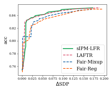
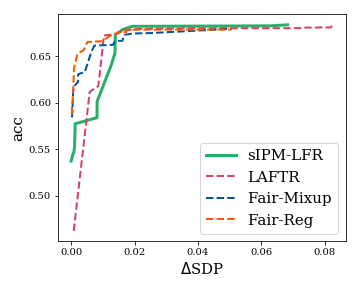
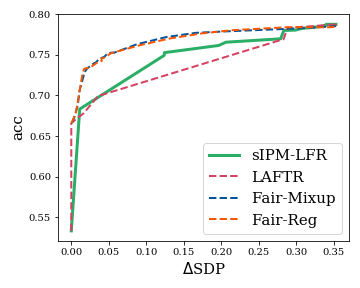
Figure D.1: Supervised LFR: Pareto-front lines between $\Delta\texttt{SDP}$ and acc on the test data of (left) Adult, (center) COMPAS, and (right) Health.

D.2 Unsupervised LFR

Additional datasets

Recently, there have been some discussions on the validity of widely-used datasets for fair AI (Ding et al., 2021; Bao et al., 2021). Furthermore, the three tabular datasets analyzed in the main paper have relatively small dimensions. Under this background, we assess the sIPM-LFR on two additional datasets: ACSIncome Toxicity.

• ACSIncome (Ding et al., 2021): This dataset is a pre-processed version of Adult dataset. Differing from Adult, ACSIncome only includes individuals above the age of 16, with working hours of at least 1hour/week in the past year, and with income of at least $100. We perform the sIPM-LFR for unsupervised LFR compared to the LAFTR on ACSIncome dataset and provide the results in Figure D.2.

• Toxicity : This dataset is a language dataset (English) containing a large number of Wikipedia comments with ratings of toxicity. For input vectors, we use the extracted representations from the encoder of a pre-trained BERT (BERT-base-uncased) (Devlin et al., 2019) provided by huggingface. For class labels, we annotate labels $1$ if the toxicity rating is over $0.5$ and $0$ otherwise. We use the encoder network with two hidden layers and the four classifiers used in Figure 2 except the 2-Sigmoid-NN. We do not use the 2-Sigmoid-NN due to its gradient vanishing problem. We perform the sIPM-LFR for unsupervised LFR compared to the LAFTR on Toxicity dataset and provide the Pareto-front lines in Figure D.3.

As can be seen in Figures D.2 and D.3, we observe similar results to those in Figure 2 for the two additional datasets in that the sIPM-LFR is better than the LAFTR in most cases.

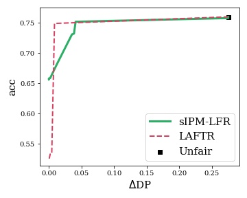
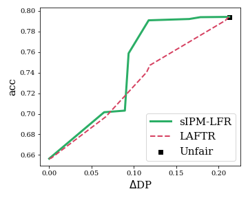
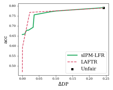
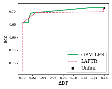
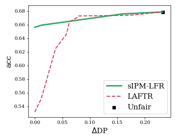
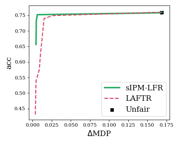
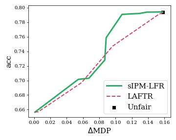
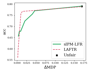
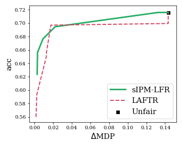
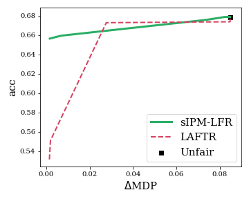
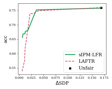
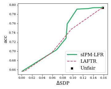
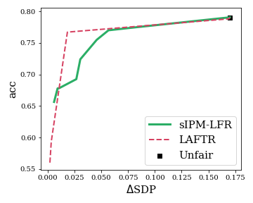
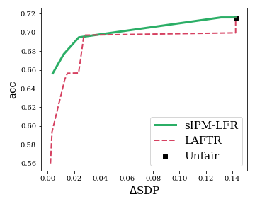
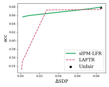
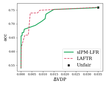
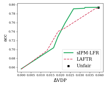
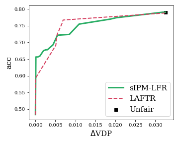
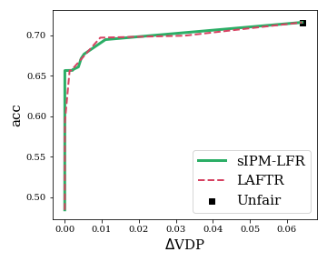
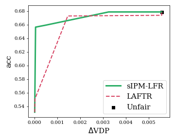
Figure D.2: Unsupervised LFR: Pareto-front lines between $\{\Delta\texttt{DP},\Delta\texttt{MDP},\Delta\texttt{SDP},\Delta\texttt{VDP}\}$ and acc on the test data of ACSIncome. (left to right) We consider the five prediction models: linear, RBF-SVM, 1-LeakyReLU-NN, 1-Sigmoid-NN, and 2-Sigmoid-NN.

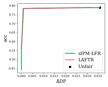
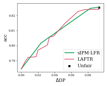
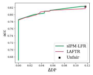
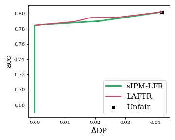
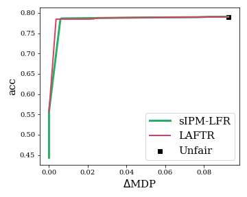
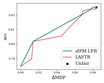
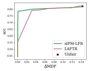
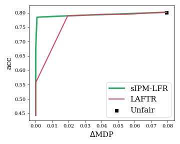
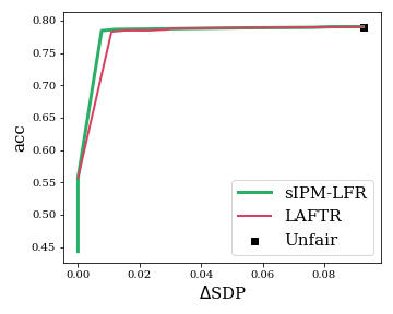
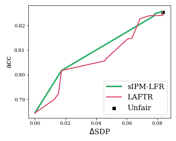
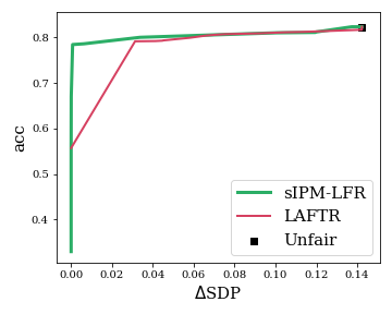
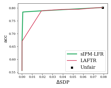
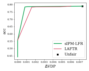
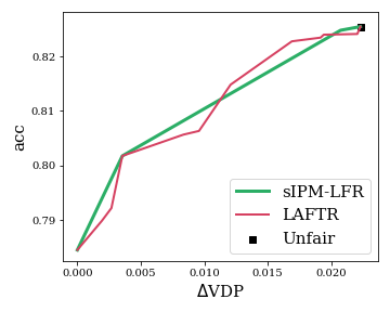
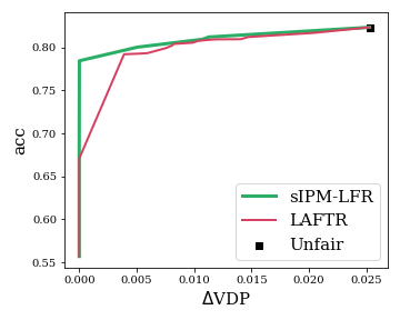
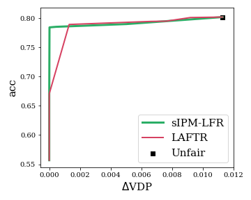
Figure D.3: Unsupervised LFR: Pareto-front lines between $\{\Delta\texttt{DP},\Delta\texttt{MDP},\Delta\texttt{SDP},\Delta\texttt{VDP}\}$ and acc on the test data of Toxicity. (left to right) We consider the four prediction models: linear, RBF-SVM, 1-LeakyReLU-NN, and 1-Sigmoid-NN.

Trade-offs between $\{\Delta\texttt{MDP},\Delta\texttt{SDP},\Delta\texttt{VDP}\}$ and acc.

We provide the Pareto-front lines (Figure D.4, D.5, and D.6) for more measures of fairness: $\Delta\texttt{MDP},\Delta\texttt{SDP},\Delta\texttt{VDP}$. We confirm that the results are similar to Figure 2.

Visualization of learned representations

Figure D.7 visualizes the representation distributions for each sensitive group derived by the sIPM-LFR with various regularization parameters. We can observe that the larger $\lambda$ becomes, the more fair the encoded representation is. That is, we can control the fairness of representation (and thus fairness of the final prediction model) nicely by choosing $\lambda$ accordingly.

Simulation for Adult with artificial $Y$

We verify our method’s superiority on unsupervised learning by an additional downstream classification task with artificial labels. We consider Adult and the artificial labels are generated as follows. We first train the encoder $h$ and decoder $f_{D}$ only with the reconstruction loss. And we draw an $m$-dimensional random vector $\gamma$ from $\mathcal{N}(0_{m},2I_{m})$ and fix it until the label generation process ends. Then, for each input sample $({\bf x},s)$, we sample a random vector $\epsilon\sim\mathcal{N}(0_{m},2I_{m})$ and generate its artificial label as $\mathbb{I}(\gamma^{\top}h({\bf x},s)+\epsilon)$. We analyze Adult with the artificial labels by comparing our method and the LAFTR, whose results are depicted in Figure D.8. We utilize the linear prediction model and consider three DP-fairness measures, $\Delta\texttt{DP},\Delta\texttt{MDP},\Delta\texttt{SDP}$. Figure D.8 shows that our method achieves consistently better trade-off results between the accuracy and DP measures.

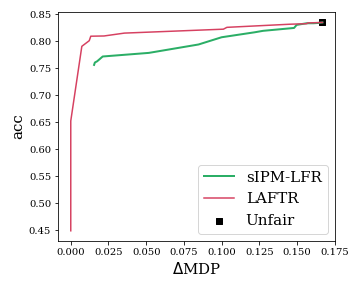
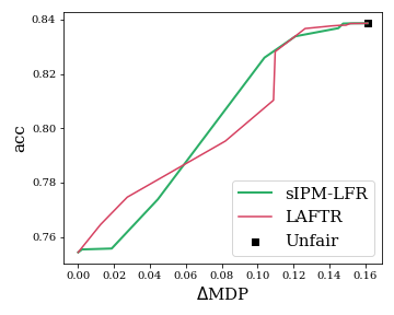
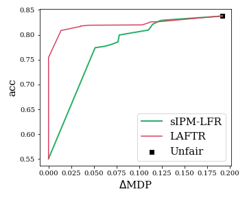
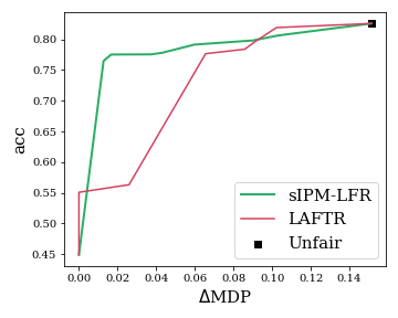
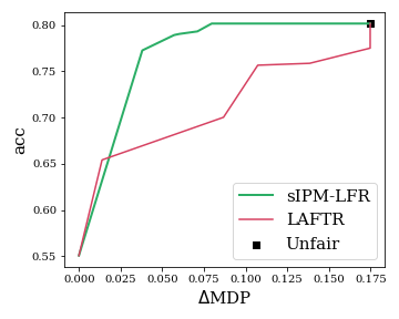
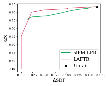
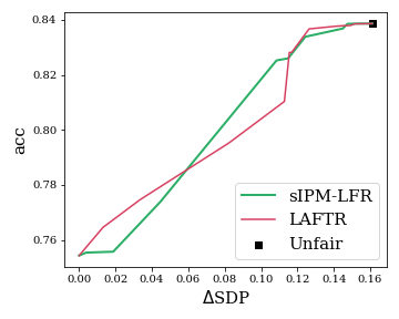
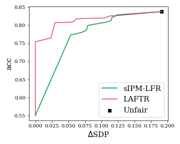
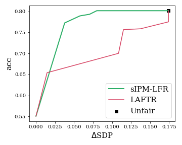
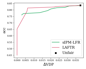
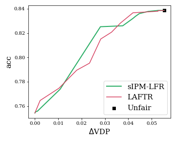
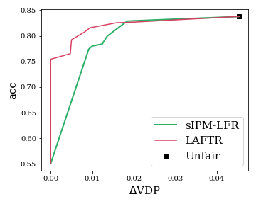
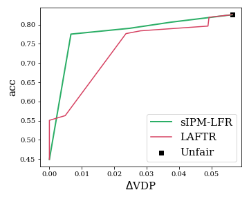
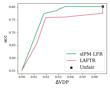
Figure D.4: Unsupervised LFR: Pareto-front lines between $\{\Delta\texttt{MDP},\Delta\texttt{SDP},\Delta\texttt{VDP}\}$ and acc on the test data of Adult. (left to right) We consider the five prediction models: linear, RBF-SVM, 1-LeakyReLU-NN, 1-Sigmoid-NN, and 2-Sigmoid-NN.

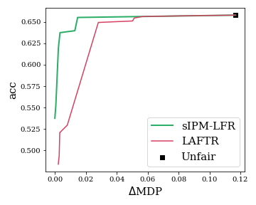
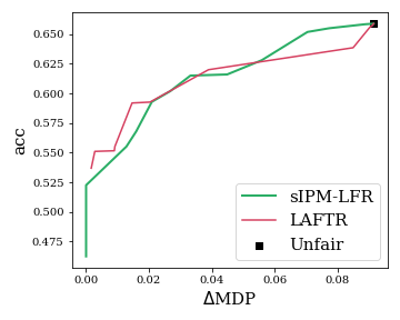
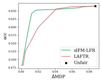
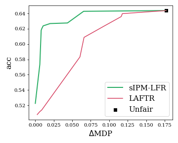
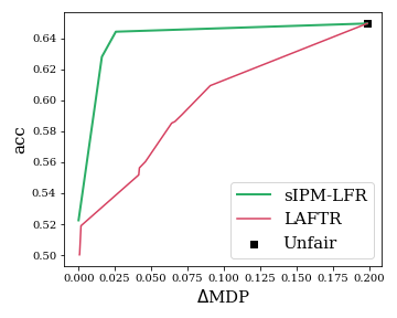
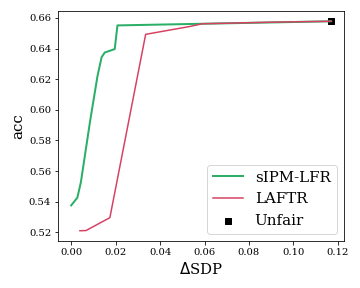
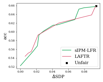
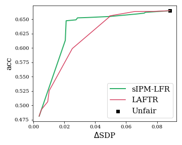
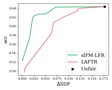
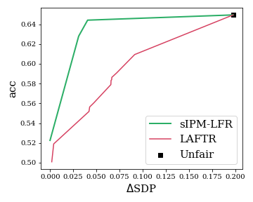
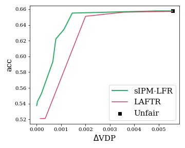
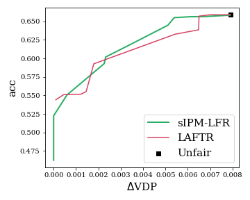
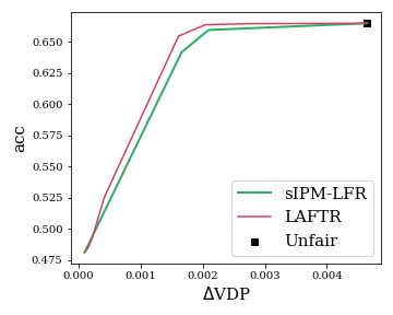
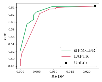
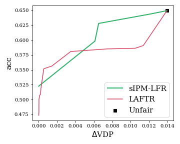
Figure D.5: Unsupervised LFR: Pareto-front lines between $\{\Delta\texttt{MDP},\Delta\texttt{SDP},\Delta\texttt{VDP}\}$ and acc on the test data of COMPAS. (left to right) We consider the five prediction models: linear, RBF-SVM, 1-LeakyReLU-NN, 1-Sigmoid-NN, and 2-Sigmoid-NN.

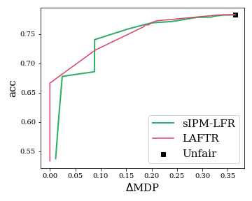
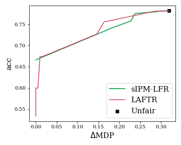
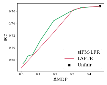
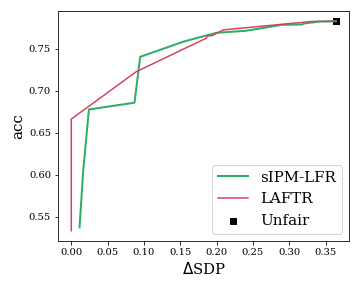
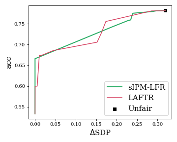
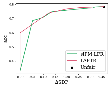
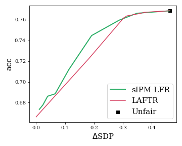
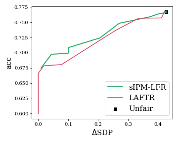
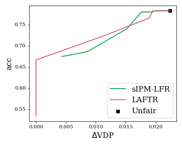
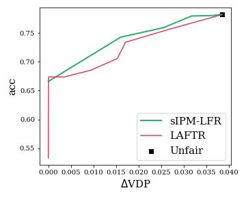
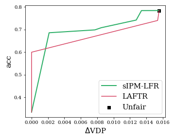
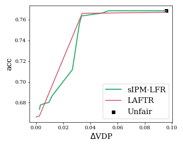
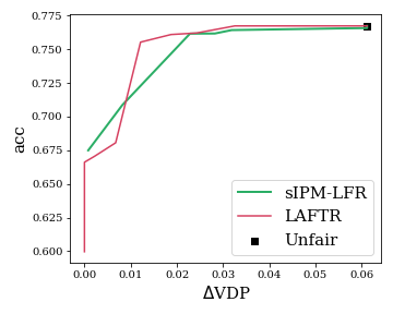
Figure D.6: Unsupervised LFR: Pareto-front lines between $\{\Delta\texttt{MDP},\Delta\texttt{SDP},\Delta\texttt{VDP}\}$ and acc on the test data of Health. (left to right) We consider the five prediction models: linear, RBF-SVM, 1-LeakyReLU-NN, 1-Sigmoid-NN, and 2-Sigmoid-NN.

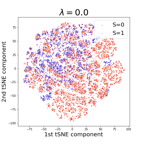
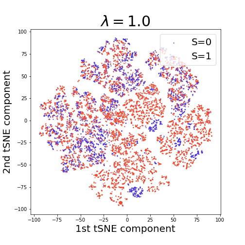
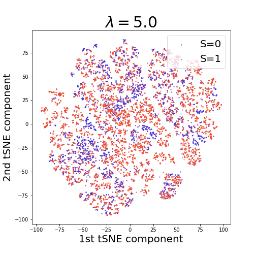
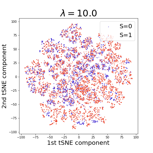
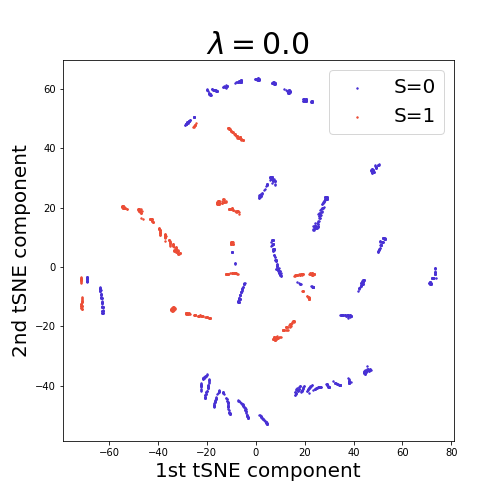
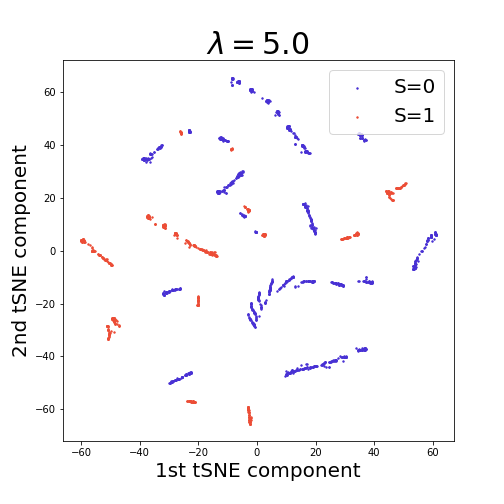
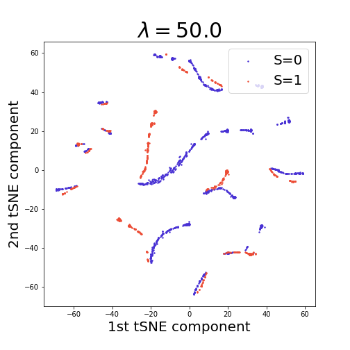
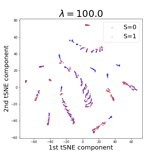
Figure D.7: Unsupervised LFR: tSNE visualization of the learned fair representation for (upper) Adult and (lower) COMPAS with various values of $\lambda$.

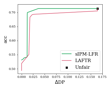
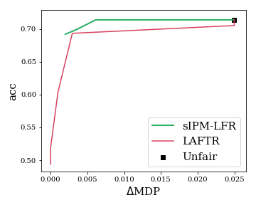
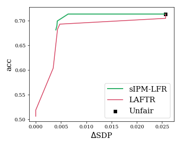
Figure D.8: Unsupervised LFR: Pareto-front lines of $\{\Delta\texttt{DP},\Delta\texttt{MDP},\Delta\texttt{SDP}\}$ (x-axis) vs. acc (y-axis) on Adult with the artificial label.

Appendix E Ablation studies

This section provides additional ablation experiments that are not included in the main manuscript.

Computation time

We conduct learning-time comparisons for the sIPM-LFR and LAFTR. As can be seen in Table E.1, sIPM-LFR requires about 20% less computation times compared to the LAFTR.

Varying the dimension of the representation

We analyze the effect of varying the representation’s dimension $m$. For each dataset, we consider two values of $m$, and compare their performances with the Pareto-front lines. As shown in Figure E.1, our method is more insensitive to the selection of $m$ compared to the LAFTR.

sIPM-LFR vs. MMD-LFR

We compare the sIPM-LFR to the FVAE (Louizos et al., 2015) which is one of the MMD-based LFR methods. Theoretically, the MMD regularization in the FVAE is also a kind of IPM that utilizes a unit ball in an RKHS as $\mathcal{V}$ (the class of discriminators). We can easily show that Theorem 4.3 and Proposition 4.4 imply that the MMD with the Gaussian kernel is upper bounded by the sIPM. That is, by controlling the parametric IPM, we expect that the MMD will be also reduced.

An obvious practical advantage of the sIPM-LFR over the FVAE would be computational simplicity. We conduct an experiment to compare the stability and performance between the sIPM-LFR and FVAE. Figure E.2 depicts the scatter points with standard errors for $\Delta\texttt{DP}$ and acc for 1-Sigmoid-NN on Adult dataset. We can check that the sIPM-LFR is more stable as well as superior compared to the FVAE, which again validates the superiority of our method.

Table E.1: Training time comparisons between the sIPM-LFR and LAFTR. We report each method’s mean and standard values with five random implementations.

Dataset	Method	Computation Time (s.e.)
Adult	sIPM-LFR ✓	100.00% (0.80%)
	LAFTR	117.48% (0.33%)
COMPAS	sIPM-LFR ✓	100.00% (3.23%)
	LAFTR	121.13% (1.77%)
Health	sIPM-LFR ✓	100.00% (0.91%)
	LAFTR	117.81% (0.53%)

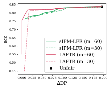
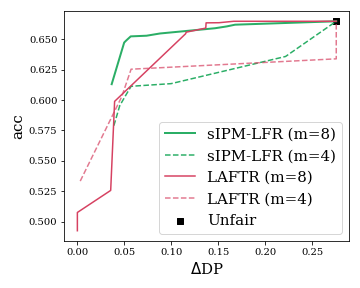
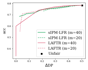
Figure E.1: Unsupervised LFR: Pareto-front lines between $\Delta\texttt{DP}$ (x-axis) and acc (y-axis) with different values of the representation dimension. We analyze three datasets: (left) Adult, (center) COMPAS, and (right) Health. We utilize the 1-LeakyReLU-NN as the prediction model.

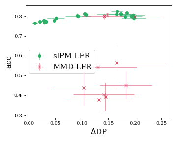
Figure E.2: Scatter plot with standard error bar of $\Delta\texttt{DP}$ and acc with various $\lambda$. Each horizontal and vertical bars present the standard errors for $\Delta\texttt{DP}$ and acc, respectively. All results are from Adult test dataset.

References

- Agarwal et al. (2018) Agarwal, A., Beygelzimer, A., Dudik, M., Langford, J., and Wallach, H. A reductions approach to fair classification. In Dy, J. and Krause, A. (eds.), Proceedings of the 35th International Conference on Machine Learning, volume 80 of Proceedings of Machine Learning Research, pp. 60–69. PMLR, 10–15 Jul 2018. URL https://proceedings.mlr.press/v80/agarwal18a.html.
- Angwin et al. (2016) Angwin, J., Larson, J., Mattu, S., and Kirchner, L. Machine bias. ProPublica, May, 23:2016, 2016.
- Ansari et al. (2020) Ansari, A. F., Scarlett, J., and Soh, H. A characteristic function approach to deep implicit generative modeling, 2020.
- Arjovsky et al. (2017) Arjovsky, M., Chintala, S., and Bottou, L. Wasserstein generative adversarial networks. In Proceedings of the 34th International Conference on Machine Learning - Volume 70, ICML’17, pp. 214–223. JMLR.org, 2017.
- Bao et al. (2021) Bao, M., Zhou, A., Zottola, S. A., Brubach, B., Desmarais, S., Horowitz, A. S., Lum, K., and Venkatasubramanian, S. It’s COMPASlicated: The messy relationship between RAI datasets and algorithmic fairness benchmarks. In Thirty-fifth Conference on Neural Information Processing Systems Datasets and Benchmarks Track (Round 1), 2021. URL https://openreview.net/forum?id=qeM58whnpXM.
- Barocas & Selbst (2016) Barocas, S. and Selbst, A. D. Big data’s disparate impact. Calif. L. Rev., 104:671, 2016.
- Barron (1993) Barron, A. R. Universal approximation bounds for superpositions of a sigmoidal function. IEEE Transactions on Information theory, 39(3):930–945, 1993.
- Calders et al. (2009) Calders, T., Kamiran, F., and Pechenizkiy, M. Building classifiers with independency constraints. In 2009 IEEE International Conference on Data Mining Workshops, pp. 13–18. IEEE, 2009.
- Chiappa (2019) Chiappa, S. Path-specific counterfactual fairness. Proceedings of the AAAI Conference on Artificial Intelligence, 33(01):7801–7808, Jul. 2019. doi: 10.1609/aaai.v33i01.33017801. URL https://ojs.aaai.org/index.php/AAAI/article/view/4777.
- Chuang & Mroueh (2021) Chuang, C.-Y. and Mroueh, Y. Fair mixup: Fairness via interpolation. 2021.
- Cortes & Vapnik (1995) Cortes, C. and Vapnik, V. Support-vector networks. Mach. Learn., 20(3):273–297, sep 1995. ISSN 0885-6125. doi: 10.1023/A:1022627411411. URL https://doi.org/10.1023/A:1022627411411.
- Creager et al. (2019) Creager, E., Madras, D., Jacobsen, J.-H., Weis, M., Swersky, K., Pitassi, T., and Zemel, R. Flexibly fair representation learning by disentanglement. In Chaudhuri, K. and Salakhutdinov, R. (eds.), Proceedings of the 36th International Conference on Machine Learning, volume 97 of Proceedings of Machine Learning Research, pp. 1436–1445. PMLR, 09–15 Jun 2019. URL https://proceedings.mlr.press/v97/creager19a.html.
- Devlin et al. (2019) Devlin, J., Chang, M.-W., Lee, K., and Toutanova, K. BERT: Pre-training of deep bidirectional transformers for language understanding. In Proceedings of the 2019 Conference of the North American Chapter of the Association for Computational Linguistics: Human Language Technologies, Volume 1 (Long and Short Papers), pp. 4171–4186, Minneapolis, Minnesota, June 2019. Association for Computational Linguistics. doi: 10.18653/v1/N19-1423. URL https://aclanthology.org/N19-1423.
- Ding et al. (2021) Ding, F., Hardt, M., Miller, J., and Schmidt, L. Retiring adult: New datasets for fair machine learning, 2021. URL https://arxiv.org/abs/2108.04884.
- Donini et al. (2018) Donini, M., Oneto, L., Ben-David, S., Shawe-Taylor, J. S., and Pontil, M. Empirical risk minimization under fairness constraints. In Advances in Neural Information Processing Systems, pp. 2791–2801, 2018.
- Dua & Graff (2017) Dua, D. and Graff, C. UCI machine learning repository, 2017. URL http://archive.ics.uci.edu/ml.
- Dwork et al. (2012) Dwork, C., Hardt, M., Pitassi, T., Reingold, O., and Zemel, R. Fairness through awareness. ITCS ’12, pp. 214–226, New York, NY, USA, 2012. Association for Computing Machinery. ISBN 9781450311151. doi: 10.1145/2090236.2090255. URL https://doi.org/10.1145/2090236.2090255.
- Edwards & Storkey (2016) Edwards, H. and Storkey, A. Censoring representations with an adversary. In International Conference in Learning Representations (ICLR2016), pp. 1–14, May 2016. URL https://iclr.cc/archive/www/doku.php%3Fid=iclr2016:main.html. 4th International Conference on Learning Representations, ICLR 2016 ; Conference date: 02-05-2016 Through 04-05-2016.
- Feldman et al. (2015) Feldman, M., Friedler, S. A., Moeller, J., Scheidegger, C., and Venkatasubramanian, S. Certifying and removing disparate impact. In proceedings of the 21th ACM SIGKDD international conference on knowledge discovery and data mining, pp. 259–268, 2015.
- Garg et al. (2019) Garg, S., Perot, V., Limtiaco, N., Taly, A., Chi, E. H., and Beutel, A. Counterfactual fairness in text classification through robustness. In Proceedings of the 2019 AAAI/ACM Conference on AI, Ethics, and Society, AIES ’19, pp. 219–226, New York, NY, USA, 2019. Association for Computing Machinery. ISBN 9781450363242. doi: 10.1145/3306618.3317950. URL https://doi.org/10.1145/3306618.3317950.
- Gibbs & Su (2002) Gibbs, A. L. and Su, F. E. On choosing and bounding probability metrics. International statistical review, 70(3):419–435, 2002.
- Gitiaux & Rangwala (2021) Gitiaux, X. and Rangwala, H. Learning smooth and fair representations. In Banerjee, A. and Fukumizu, K. (eds.), Proceedings of The 24th International Conference on Artificial Intelligence and Statistics, volume 130 of Proceedings of Machine Learning Research, pp. 253–261. PMLR, 13–15 Apr 2021. URL https://proceedings.mlr.press/v130/gitiaux21a.html.
- Goodfellow et al. (2014) Goodfellow, I., Pouget-Abadie, J., Mirza, M., Xu, B., Warde-Farley, D., Ozair, S., Courville, A., and Bengio, Y. Generative adversarial nets. In Ghahramani, Z., Welling, M., Cortes, C., Lawrence, N., and Weinberger, K. Q. (eds.), Advances in Neural Information Processing Systems, volume 27. Curran Associates, Inc., 2014. URL https://proceedings.neurips.cc/paper/2014/file/5ca3e9b122f61f8f06494c97b1afccf3-Paper.pdf.
- Hardt et al. (2016) Hardt, M., Price, E., and Srebro, N. Equality of opportunity in supervised learning. In Advances in neural information processing systems, pp. 3315–3323, 2016.
- Kantorovich & Rubinstein (1958) Kantorovich, L. and Rubinstein, G. S. On a space of totally additive functions. Vestnik Leningrad. Univ, 13:52–59, 1958.
- Kleinberg et al. (2018) Kleinberg, J., Ludwig, J., Mullainathan, S., and Rambachan, A. Algorithmic fairness. In Aea papers and proceedings, volume 108, pp. 22–27, 2018.
- Kusner et al. (2017) Kusner, M. J., Loftus, J., Russell, C., and Silva, R. Counterfactual fairness. In Guyon, I., Luxburg, U. V., Bengio, S., Wallach, H., Fergus, R., Vishwanathan, S., and Garnett, R. (eds.), Advances in Neural Information Processing Systems, volume 30. Curran Associates, Inc., 2017. URL https://proceedings.neurips.cc/paper/2017/file/a486cd07e4ac3d270571622f4f316ec5-Paper.pdf.
- Lohaus et al. (2020) Lohaus, M., Perrot, M., and Luxburg, U. V. Too relaxed to be fair. In III, H. D. and Singh, A. (eds.), Proceedings of the 37th International Conference on Machine Learning, volume 119 of Proceedings of Machine Learning Research, pp. 6360–6369. PMLR, 13–18 Jul 2020. URL https://proceedings.mlr.press/v119/lohaus20a.html.
- Louizos et al. (2015) Louizos, C., Swersky, K., Li, Y., Welling, M., and Zemel, R. The variational fair autoencoder, 2015. URL https://arxiv.org/abs/1511.00830.
- Madras et al. (2018) Madras, D., Creager, E., Pitassi, T., and Zemel, R. S. Learning adversarially fair and transferable representations. In ICML, 2018.
- Man (2017) Man, Y. K. On computing the vandermonde matrix inverse. In Proceedings of the World Congress on Engineering, volume 1, 2017.
- McCullagh (1994) McCullagh, P. Does the moment-generating function characterize a distribution? The American Statistician, 48(3):208–208, 1994.
- Mehrabi et al. (2019) Mehrabi, N., Morstatter, F., Saxena, N., Lerman, K., and Galstyan, A. A survey on bias and fairness in machine learning. arXiv preprint arXiv:1908.09635, 2019.
- Mukherjee et al. (2020a) Mukherjee, D., Yurochkin, M., Banerjee, M., and Sun, Y. Two simple ways to learn individual fairness metrics from data. In Proceedings of the 37th International Conference on Machine Learning, pp. 7097–7107, 2020a.
- Mukherjee et al. (2020b) Mukherjee, D., Yurochkin, M., Banerjee, M., and Sun, Y. Two simple ways to learn individual fairness metrics from data. In Proceedings of the 37th International Conference on Machine Learning, pp. 7097–7107, 2020b.
- Noh et al. (2015) Noh, H., Hong, S., and Han, B. Learning deconvolution network for semantic segmentation. In Proceedings of the IEEE international conference on computer vision, pp. 1520–1528, 2015.
- Quadrianto et al. (2019a) Quadrianto, N., Sharmanska, V., and Thomas, O. Discovering fair representations in the data domain. In Proceedings of the IEEE/CVF Conference on Computer Vision and Pattern Recognition (CVPR), June 2019a.
- Quadrianto et al. (2019b) Quadrianto, N., Sharmanska, V., and Thomas, O. Discovering fair representations in the data domain. In Proceedings of the IEEE/CVF Conference on Computer Vision and Pattern Recognition, pp. 8227–8236, 2019b.
- Ruoss et al. (2020) Ruoss, A., Balunovic, M., Fischer, M., and Vechev, M. Learning certified individually fair representations. In Advances in Neural Information Processing Systems 33. 2020.
- Sharifi-Malvajerdi et al. (2019) Sharifi-Malvajerdi, S., Kearns, M., and Roth, A. Average individual fairness: Algorithms, generalization and experiments. In Advances in Neural Information Processing Systems, volume 32, 2019. URL https://proceedings.neurips.cc/paper/2019/file/0e1feae55e360ff05fef58199b3fa521-Paper.pdf.
- Steinwart & Christmann (2008) Steinwart, I. and Christmann, A. Support vector machines. Springer Science & Business Media, 2008.
- Villani (2008) Villani, C. Optimal transport: Old and new. 2008.
- Wu et al. (2019a) Wu, Y., Zhang, L., and Wu, X. On convexity and bounds of fairness-aware classification. In The World Wide Web Conference, WWW ’19, pp. 3356–3362, New York, NY, USA, 2019a. Association for Computing Machinery. ISBN 9781450366748. doi: 10.1145/3308558.3313723. URL https://doi.org/10.1145/3308558.3313723.
- Wu et al. (2019b) Wu, Y., Zhang, L., and Wu, X. Counterfactual fairness: Unidentification, bound and algorithm. In Proceedings of the Twenty-Eighth International Joint Conference on Artificial Intelligence, IJCAI-19, pp. 1438–1444. International Joint Conferences on Artificial Intelligence Organization, 7 2019b. doi: 10.24963/ijcai.2019/199. URL https://doi.org/10.24963/ijcai.2019/199.
- Xu et al. (2018) Xu, D., Yuan, S., Zhang, L., and Wu, X. Fairgan: Fairness-aware generative adversarial networks. In 2018 IEEE International Conference on Big Data (Big Data), pp. 570–575, 2018. doi: 10.1109/BigData.2018.8622525.
- Xu et al. (2020) Xu, R., Cui, P., Kuang, K., Li, B., Zhou, L., Shen, Z., and Cui, W. Algorithmic decision making with conditional fairness. Proceedings of the 26th ACM SIGKDD International Conference on Knowledge Discovery Data Mining, Jul 2020. doi: 10.1145/3394486.3403263. URL http://dx.doi.org/10.1145/3394486.3403263.
- Yona & Rothblum (2018) Yona, G. and Rothblum, G. Probably approximately metric-fair learning. In Dy, J. and Krause, A. (eds.), Proceedings of the 35th International Conference on Machine Learning, volume 80 of Proceedings of Machine Learning Research, pp. 5680–5688, Stockholmsmässan, Stockholm Sweden, 10–15 Jul 2018. PMLR.
- Yukich et al. (1995) Yukich, J. E., Stinchcombe, M. B., and White, H. Sup-norm approximation bounds for networks through probabilistic methods. IEEE Transactions on Information Theory, 41(4):1021–1027, 1995.
- Zafar et al. (2017) Zafar, M. B., Valera, I., Rogriguez, M. G., and Gummadi, K. P. Fairness constraints: Mechanisms for fair classification. In Artificial Intelligence and Statistics, pp. 962–970, 2017.
- Zeiler (2012) Zeiler, M. D. Adadelta: An adaptive learning rate method. CoRR, abs/1212.5701, 2012. URL http://dblp.uni-trier.de/db/journals/corr/corr1212.html#abs-1212-5701.
- Zemel et al. (2013) Zemel, R., Wu, Y., Swersky, K., Pitassi, T., and Dwork, C. Learning fair representations. In Dasgupta, S. and McAllester, D. (eds.), Proceedings of the 30th International Conference on Machine Learning, volume 28 of Proceedings of Machine Learning Research, pp. 325–333, Atlanta, Georgia, USA, 17–19 Jun 2013. PMLR. URL https://proceedings.mlr.press/v28/zemel13.html.
- Zeng et al. (2021) Zeng, Z., Islam, R., Keya, K. N., Foulds, J., Song, Y., and Pan, S. Fair representation learning for heterogeneous information networks, 2021.