Role of Gauss-Bonnet corrections in a DGP brane gravitational collapse

Abstract

An Oppenheimer-Snyder (OS)-type collapse is considered for a Dvali-Gabadadze-Porrati (DGP) brane, whereas a Gauss-Bonnet (GB) term is provided for the bulk. We study the combined effect of the DGP induced gravity plus the GB curvature, regarding any modification of the general relativistic OS dynamics. Our paper has a twofold objective. On the one hand, we investigate the nature of singularities that may arise at the collapse end state. It is shown that all dynamical scenarios for the contracting brane would end in one of the following cases, depending on conditions imposed: either a central shell-focusing singularity or what we designate as a “sudden collapse singularity.” On the other hand, we also study the deviations of the exterior spacetime from the standard Schwarzschild geometry, which emerges in our modified OS scenario. Our purpose is to investigate whether a black hole always forms regarding this brane world model. We find situations where a naked singularity emerges instead.

I Introduction

One of the most impressive features in relativistic astrophysics is the occurrence of continual gravitational collapse of supermassive stars due to their own gravitational fields. This provides a framework toward understanding the basic mechanism for the formation of white dwarfs, neutron stars, then possibly supermassive black holes [1, 2]. In particular, one of the main consequences of general relativistic gravitational collapse is the formation of central singularities at the collapsing final state, where the gravitational field and, consequently, the spacetime scalar curvature are predicted to diverge.

An important inquiry that may arise in this context is whether there exist circumstances that avoid the formation of the black hole event horizon prior to the occurrence of the central singularity, allowing it to be visible to the external world. It turns out that, despite the theoretical predictions for the existence of naked singularity solutions in general relativity (GR), Penrose argued, through his cosmic censorship conjecture [3], that such situation would not occur: central singularities should be hidden within event horizons and therefore cannot be observed from the rest of the spacetime. The previous appraisal notwithstanding, at a more fundamental level it is believed that a singularity is indeed not a location where quantities really become infinite, but instead where GR merely breaks down. Thereby, GR should be superseded by a robust singularity-free gravitational theory (as yet unknown, quantum theory of gravity). In the past decades, there has been enormous efforts in order to put forward a more complete theory for gravitation, which would be free of such obstacles.

Higher-dimensional brane world models [4, 5, 6, 7, 8], due to the presence of both bulk and brane curvature terms in their actions, have a different gravitational behavior from their general relativistic counterpart [9, 10]. They provide interesting extensions of our parameter space for gravitational theories. In particular, within cosmological and astrophysical contexts, brane world models admit spacetime singularities of rather unusual form and nature [11, 12, 13, 14]. Among these models, there are scenarios of specific interest. On the one hand, we have brane gravity proposed by Dvali et al. (known as the DGP induced-gravity model), in which the brane action constitutes an alteration (with respect to the Einstein-Hilbert term for GR), so that it provides a low energy (or infrared) modification through an induced-gravity term [5]. On the other hand, we can also consider Gauss-Bonnet (GB) (higher-order curvature) corrections, which are introduced for the bulk [15, 16, 17, 18, 19]. So, whereas DGP features play at infrared range, the GB elements change gravity at high energy (or ultraviolet). These two additions allow us to broaden the scope of research with respect to gravitational collapse, beyond and encompassing GR as a suitable limit, possibly suggesting a peculiar phenomenology from the quantum gravity sector.

The previous paragraphs set the context of our herewith reported research, with the one just above closely assisting in defining our purposes. Let us be more precise. The gravitational collapse of a stellar object was first studied by Oppenheimer and Snyder [20] in the context of GR. By considering a homogeneous spherically symmetric matter cloud with vanishing internal pressures and zero rotation, they showed that the cloud collapses simultaneously to a (central) spacetime singularity, covered within a black hole event horizon. This mechanism has been extended later to more general models of gravitational collapse in GR (see [2, 21] and references therein) and alternative theories of gravity [22, 23, 24, 25], namely, brane induced gravity [26, 27] including GB corrections [28], as well as in quantum gravity approaches [29, 30, 31, 32, 33, 34, 35, 36, 37, 38, 39].

Further regarding our setup, let us mention that a supermassive star can both be large and have huge energy density. That motivates and suggests that it should be of specific interest to investigate, for instance, how the combination of DGP brane gravity with GB terms can alter the final state, possibly with asymptotic states rather different from those within a GR framework. Therefore, questions such as how the influence of higher-dimensional effects would modify the evolution of event horizons and formation of central singularity are sufficient to enthuse us to investigate gravitational collapse as described above. In this sense, it has been shown that a collapse in the DGP-GB system can avoid the formation of a black hole. Concretely, if one considers a large scale system (the initial matter configuration assumed to be distributed within a large radius) that corresponds to a marginally bound [$k=0$, here $k$ is a constant in Friedmann-Lemaître-Robertson-Walker (FLRW) metric which represents the curvature of the space] case, then the collapse outcome depends on the initial mass of the system, and a “naked sudden singularity” can emerge before the collapse process reaches the vanishing physical radius $R=0$ point; see Ref. [28] for details. In our present paper, we develop instead from a generalized initial configuration which has been assumed to include the bound collapse ($k=1$), and, as it will be discussed in the rest of the paper, new plausible scenarios have been obtained.

Thus, our current paper has a twofold objective. On the one hand, we study the effect of the DGP brane world model, containing a GB curvature in the bulk, regarding any modification of the general relativistic Oppenheimer-Snyder (OS) [20] collapse. Concretely, we investigate the nature of singularities that may arise at the collapse end state. We find that, depending on conditions that we will make explicit, two type of singularities can happen: a central shell-focusing singularity or what we designate as a sudden collapse singularity (SCS). In addition, our other purpose is to identify any deviation of the exterior spacetime from the standard Schwarzschild black hole, which emerges in the relativistic OS model.

Motivated as we described in the previous paragraphs, we thus organized our paper as follows. In Sec. II, we will present our model of gravitational collapse, by considering a closed FLRW for the contracting brane, containing a dust fluid as matter content, with a GB term in the bulk. We will then present the evolution equation of the collapse on the brane and provide different classes of solutions. In Sec. III, we discuss the physically relevant solutions for the evolution of the contracting brane and present the emergence of a specific type of singularity at which, for a nonzero physical radius, the energy density of the brane remains finite, while the time derivative of the Hubble rate diverges. In Sec. IV, the matching condition at the boundary of the collapsing object will be investigated and possible solutions to the exterior geometry at the final state of the collapse will be determined. Finally, in Sec. V, we present our conclusion and a discussion of our work.

II Gravitational collapse in the DGP-GB model

We consider the DGP brane world model in which a GB curvature term is present in the five-dimensional Minkowski bulk containing a FLRW brane with an induced-gravity term. Moreover, all the energy-momentum is localized on the four-dimensional brane. Therefore, the total gravitational action can be written as

$$S =\frac{1}{2}\int dx^{5}\sqrt{-g^{(5)}}\,M^{3}_{(5)}\left[{\cal R}_{(5)}+\alpha\mathcal{L}_{\rm GB}\right]+\frac{1}{2}\int dx^{4}\sqrt{-g}\,M^{2}_{(4)}\left({\cal R}_{(4)}+{\cal L}_{\rm matt}\right),$$ (1)

where $\mathcal{L}_{\rm GB}$ is the Lagrangian density of the GB sector

$$\mathcal{L}_{\rm GB}={\cal R}_{(5)}^{2}-4{\cal R}_{(5)ab}{\cal R}_{(5)}^{ab}+{\cal R}_{(5)abcd}{\cal R}_{(5)}^{abcd}.$$ (2)

Here, $g^{(5)}$ and $g$ denote, respectively, determinants of the metric in the bulk and the induced metric on the brane. The couplings $M_{(5)}^{-3}=\kappa^{2}_{(5)}$ and $M_{(4)}^{-2}=\kappa^{2}_{(4)}$ are respectively, the four- and five-dimensional gravitational constants. Moreover, $\alpha>0$ is the GB coupling constant. The standard DGP model is the special case with $\alpha=0$ and possesses a crossover scale, defined by $r_{c}=\kappa^{2}_{(5)}/2\kappa^{2}_{(4)}$, which marks the transition from the four-dimensional brane to the five-dimensional bulk.

We consider an OS model for gravitational collapse on the brane. It consists of a spacetime manifold $\mathbb{R}\times\Sigma$ on the brane, where $\mathbb{R}$ represents the time direction and $\Sigma$ is a homogeneous and isotropic three-manifold bearing a dust cloud. The homogeneity and isotropy imply that $\Sigma$ must be a maximally symmetric space, so the space is spherically symmetric. Then, the spacetime geometry within this spherically symmetric cloud is described by the comoving coordinates $(t,r,\theta,\varphi)$ [20]

$$ds^{2}=-dt^{2}+\frac{a^{2}(t)}{\left(1+kr^{2}/4\right)^{2}}\Big{[}dr^{2}+r^{2}d\Omega^{2}\Big{]},$$ (3)

where $t$ is the proper time, with $a(t)$ being the scale factor of the collapse, and $d\Omega^{2}$ is the line element of the standard unit two-sphere. Moreover, $R$ is denoted to be the physical radius, given by

$$R(t,r)=\frac{ra(t)}{1+kr^{2}/4}\,=:\,\mathbf{r}a(t)\,.$$ (4)

In GR, the case $k=0$ describes a marginally bound collapse, in which shells at infinity have zero initial velocity [i.e., $\dot{R}(t_{0},r)=0$]. The case in which $k=-1$ states an unbound collapse whose shells at infinity have positive initial velocity [$\dot{R}(t_{0},r)>0$]. Finally, the case $k=+1$ represents a bound collapse for which shells at infinity have negative initial velocity [$\dot{R}(t_{0},r)<0$].

The generalized Friedmann equation of a spatially closed (i.e., with $k=+1$) DGP brane with a GB term in a Minkowski bulk [defined in Eq. (1)] reads [9]

$$h^{2}=\frac{\kappa_{(5)}^{2}}{6r_{c}}\rho+\frac{\epsilon}{r_{c}}\left(1+\frac{8}{3}\alpha h^{2}\right)h,$$ (5)

where, $h$ is defined in terms of the parameter $H$ of the brane as

$$h^{2}\ :=\ H^{2}+\frac{k}{a^{2}}\,.$$ (6)

For the case $\alpha=0$ and $k=0$, Eq. (5) reduces to the Friedmann equation in the standard DGP model [4]. The parameter $\epsilon$ can take the values $\epsilon=\pm 1$; the $(-)$ sign for $\epsilon$ can be visualized as the interior of the space bounded by a hyperboloid (the brane), whereas the $(+)$ sign corresponds to the exterior. Moreover, $\rho$ stands for the total energy density of the brane. For an evolving brane, containing a perfect fluid with an equation of state parameter $w=\gamma-1$, which represents a collapsing star, the energy density is well described by

$$\rho=\rho_{0}\left(\frac{a_{0}}{a}\right)^{3\gamma}\,,$$ (7)

where $\gamma,\rho_{0}$ and $a_{0}$ are constants. To compare our model to an OS-type collapse, we are interested in a (pressureless) dust fluid, so henceforth we will set $\gamma=1$.

It is convenient to introduce the following dimensionless variables in order to analyze the evolution of the Hubble rate as a function of the energy density of the brane [12]:

$$\bar{h}:=\frac{8}{3}\frac{\alpha}{r_{c}}h,\quad\bar{\rho}:=\frac{32}{27}\frac{\kappa_{(5)}^{2}\alpha^{2}}{r_{c}^{3}}\rho,\quad b:=\frac{8}{3}\frac{\alpha}{r_{c}^{2}}\,.\quad$$ (8)

Using these new variables, the evolution equation (5) for the $(-)$ and $(+)$ branches become

$${\bar{h}}^{3}+{\bar{h}}^{2}+b\bar{h}-\bar{\rho}=0\quad{\rm for~{}the~{}(-)~{}branch},$$ (9a)

$${\bar{h}}^{3}-{\bar{h}}^{2}+b\bar{h}+\bar{\rho}=0\quad{\rm for~{}the~{}(+)~{}branch}.\quad$$ (9b)

By solving these equations for $\bar{h}$, we can obtain the solutions to the Hubble rate as

$$\bar{H}\,=\,-\sqrt{\bar{h}^{2}-\frac{\bar{k}^{2}}{a^{2}}}\,,$$ (10)

where we have defined

$$\bar{H}\,:=\,\frac{8}{3}\frac{\alpha}{r_{c}}H=br_{c}H\,,\quad{\rm and}\quad\bar{k}^{2}\,:=\,kb^{2}r_{c}^{2}\,.$$ (11)

We note that $\bar{H}$ above is always real and negative when the argument under the square root is positive. The two cubic equations (9a) and (9b) can be transformed to one another by changing the parameter therein as $\bar{h}\rightarrow-\bar{h}$. Thus, positive solutions of the first equation correspond to the negative solutions of the second one, and vice versa. Interestingly, the solutions $\bar{h}$ in the expression (10) under the square root is of quadratic form, which indicates that considering either of the branches leads to identical solutions for the Hubble rate [14]. Therefore, we will henceforth consider only the first equation [the one corresponding to the $(-)$ branch] and will present the solutions of the second equation only briefly in Table 1. Nevertheless, we should notice that, as we will explain carefully in what follows, having the same solution for $\bar{h}$ does not necessarily lead to the same end state for the collapse. In fact, other elements will also play an important role as we will explain.

Let assume that $\bar{k}>0$. Then, at the initial configuration, positiveness of the argument under the square root implies that $|\bar{h}(t_{0})|$ should be slightly larger than $\bar{k}/a_{0}$, where the collapsing cloud has a maximum size at $a(t_{0})=a_{0}$. Since the scale factor decreases as the collapse evolves, then in order to keep the argument under the square root positive, the parameter $|\bar{h}|$ should increase toward $a=0$ (and identically zero physical radius, $R=0$). This means that $|\bar{h}|$ has a minimum value at the initial hypersurface, i.e., $|\bar{h}_{0}|=|\bar{h}|_{\rm min}$. This minimum should satisfy the initial condition

$$\bar{h}_{0}\gtrsim\frac{\bar{k}}{a_{0}}\,\quad\quad{\rm or}\quad\quad\bar{h}_{0}\lesssim-\frac{\bar{k}}{a_{0}}\,.$$ (12)

Then, for all $t>t_{0}$, the physically reasonable solutions for $\bar{h}(t)$ are those that hold the condition

$$|\bar{h}(t)|\geq\frac{\bar{k}}{a(t)}\,.$$ (13)

In order to determine the number of real roots of the cubic equations (9) it is helpful to define the discriminant function $N$ as [41, 14]

$$N=Q^{3}+S^{2},$$ (14)

where $Q$ and $S$ are

$$Q:=\frac{1}{3}\left(b-\frac{1}{3}\right),\quad\quad S:=\frac{1}{6}b+\frac{1}{2}\bar{\rho}-\frac{1}{27}\,.$$ (15)

For later convenience, in analyzing the number of physical solutions of the modified Friedmann equation, we rewrite $N$ as [14]

$$N=\frac{1}{4}(\bar{\rho}-\bar{\rho}_{A})(\bar{\rho}-\bar{\rho}_{B}),$$ (16)

where

$$\bar{\rho}_{A}\, := \,\frac{2}{27}\left[1+\sqrt{(1-3b)^{3}}\right]-\frac{b}{3}\,,$$ (17a)

$$\bar{\rho}_{B}\, := \,\frac{2}{27}\left[1-\sqrt{(1-3b)^{3}}\right]-\frac{b}{3}\,.$$ (17b)

The number of roots of Eqs. (9) is determined by the sign of $N$: If $N$ is positive, there exists a unique real root. If $N$ is negative, there are three real solutions, and for vanishing $N$, all roots are real and at least two are equal.

From Eq. (16) it is clear that the sign of $N$ depends on the value of the energy density of the brane $\bar{\rho}$ with respect to the parameters $\bar{\rho}_{A}$ and $\bar{\rho}_{B}$. Moreover, $\bar{\rho}_{A}$ and $\bar{\rho}_{B}$ are defined in terms of the parameter $b$. Then, in order to determine the sign of $N$ and, consequently, the number of solutions of the modified Friedmann equations for the $(-)$ and $(+)$ branches, it is convenient to distinguish four ranges for the values of $b$, as (A) the range $0<b<\frac{1}{4}$, (B) the range $\frac{1}{4}\leq b<\frac{1}{3}$, (C) the value $b=\frac{1}{3}$, and, finally, (D) the range $b>\frac{1}{3}$.

In the following subsections, we will study the possible solutions of the Friedmann equations (9) for different ranges of $b$, namely A–D.

II.1 The case $0<b<\frac{1}{4}$

In this case, the values of $\bar{\rho}_{A}$ and $\bar{\rho}_{B}$ are real and, furthermore, $\bar{\rho}_{A}>0$ and $\bar{\rho}_{B}<0$. Then, the number of real roots of the cubic equation (9a) depend on the minimum energy density $\rho_{0}$ (of the dust fluid) on the brane. Let us define the dimensionless energy density $\bar{\rho}_{0}$ of the collapsing fluid as

$$\bar{\rho}_{0}\,:=\,\frac{32}{27}\frac{\kappa_{(5)}^{2}\alpha^{2}}{r_{c}^{3}}\rho_{0}\,=\,\frac{\kappa_{(4)}^{2}}{3}b^{2}r_{c}^{2}\rho_{0}.$$ (18)

Then, different situations for the roots can be distinguished within two cases: $\bar{\rho}_{0}>\bar{\rho}_{A}$ and $\bar{\rho}_{0}\leq\bar{\rho}_{A}$. In what follows in this subsection we will analyze the possible real solutions of (9a) for these two initial conditions.

II.1.1 The condition $\bar{\rho}_{0}>\bar{\rho}_{A}$

For this choice of initial condition at any $t>t_{0}$ in the future, the condition $\bar{\rho}>\bar{\rho}_{A}$ will always hold because, in the collapse process, the energy density of the dust is incremental as it moves from the initial configuration toward $R=0$. Thus, the function $N$ will always remain positive, thereby, there exists a unique real solution for (9a),

$$\bar{h}_{1}(\eta)=\frac{1}{3}\left[2\sqrt{1-3b}\cosh\left(\frac{\eta}{3}\right)-1\right],$$ (19)

where the parameter $\eta$ is defined as

$$\quad\cosh(\eta)\coloneqq\frac{S}{\sqrt{-Q^{3}}}~{},\quad\quad\sinh(\eta)\coloneqq\sqrt{-\frac{N}{Q^{3}}}\,.$$ (20)

Using the first relation in Eq. (20), we can find an expression for the energy density of the brane in terms of $\eta$ as

$$\bar{\rho}_{1}(\eta)\,=\,\frac{2}{27}\left[1+\sqrt{(1-3b)^{3}}\cosh(\eta)\right]-\frac{b}{3}\,.\quad\quad$$ (21)

From $\bar{\rho}_{1}(\eta)\geq\bar{\rho}_{0}>\bar{\rho}_{A}$, it follows that the parameter $\eta$ is constrained by $\cosh(\eta)\geq\cosh(\eta_{0})>\cosh(\eta_{A})$. This yields a lower bound on $\eta$ as $\eta\geq\eta_{0}>\eta_{A}$, where $\eta_{A}$ and $\eta_{0}$ are given by

$$\cosh(\eta_{A})\, = \,\frac{9b+27\bar{\rho}_{A}-2}{2\sqrt{(1-3b)^{3}}}\,,$$ (22a)

$$\cosh(\eta_{0})\, = \,\frac{9b+27\bar{\rho}_{0}-2}{2\sqrt{(1-3b)^{3}}}\,.$$ (22b)

Now, Eq. (22a) yields $\eta_{A}=0$, thereby, the solution $\bar{h}_{1}(\eta_{A})\equiv\bar{h}_{A}$ is determined as

$$\bar{h}_{A}\coloneqq\frac{1}{3}\left[2\sqrt{1-3b}-1\right].$$ (23)

Likewise, by using the energy density (21) into the Eq. (7) the scale factor is obtained in terms of $\eta$ as

$$a_{1}(\eta) = a_{0}\left(\frac{\bar{\rho}_{0}}{\bar{\rho}_{1}(\eta)}\right)^{\frac{1}{3}}.\quad\qquad$$ (24)

As $\eta$ increases, $\bar{\rho}_{1}(\eta)$ increases as well so the scale factor decreases toward zero, where $\eta$ diverges.

The condition (13) implies that, since the scale factor $a_{1}(t)$ decreases by time as collapse proceeds, the solution $\bar{h}_{1}(\eta)$ should increase much faster than $\bar{k}/a_{1}(\eta)$. It turns out that, since $\bar{h}_{1}(\eta)$ was initially positive valued, it should remain positive for all times in the future. By imposing the initial condition (12) into the solution (19), this produces a more restricted range for the parameter $\eta$; it is $\eta_{0}>\eta_{\rm min}>0$, where $\eta_{\rm min}$ is given by

$$\cosh\left(\frac{\eta_{\rm min}}{3}\right)\coloneqq\frac{3(\bar{k}/a_{0})+1}{2\sqrt{1-3b}}\,.$$ (25)

On the other hand, $\bar{h}_{1}(\eta)$ should belong to the range

$$\bar{h}_{1}(\eta_{0})>\bar{h}_{1}(\eta)>\bar{h}_{\rm 1min}\,,$$ (26)

where, $\bar{h}_{\rm 1min}\equiv\bar{k}/a_{0}$. Thus, $\bar{H}_{1}(\eta)$ is determined by setting Eqs. (19) and (24) into Eq. (10):

$$\bar{H}_{1}(\eta)\,=\,-\sqrt{\bar{h}_{1}^{2}(\eta)-\frac{\bar{k}^{2}}{a_{1}^{2}(\eta)}}\,.$$ (27)

Because both terms under the square root of Eq. (27) increase from the initial state, we expect two possible scenarios for the evolution of the collapse. The first is a case in which the term $\bar{h}_{1}(\eta)$ increases faster than the second term $\bar{k}/a_{1}(\eta)$, so that, as the collapse progresses toward a “centering” point, $\bar{H}_{1}$ blows up. The other scenario is that the second term in Eq. (27) increases faster than the first term so that at some moment in the future, the two terms cancel each other and $\bar{H}_{1}$ vanishes. Nevertheless, the numerical analysis shown in Fig. 1 indicates that initially, when the collapse starts [i.e., $\bar{H}_{1}(t_{0})\lesssim 0$] and satisfies the condition (26), this condition will continue to hold through the whole collapsing process. Therefore, as the collapse proceeds, the first term in Eq. (27) increases faster than the second term so that, $\bar{H}_{1}(\eta)$ will blow up (with a minus sign) at the vicinity of $a=0$.

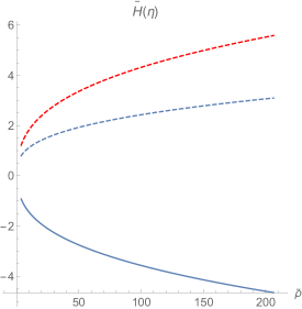
Figure 1: The evolution of the (dimensionless) $\bar{H}_{1}(\eta)$ in terms of $\bar{\rho}$, in the range of parameters $0<b<1/4$ and for the initial condition $\bar{\rho}_{0}>\bar{\rho}_{A}$: it is shown that for all $\eta>\eta_{\rm min}$, the first term, $\bar{h}_{1}(\eta)$, in Eq. (27) (dashed red curve) increases faster than the second term, $\bar{k}/a_{1}(\eta)$ (dashed blue curve), so $\bar{H}_{1}(\eta)$ (solid blue curve) blows up (with a minus sign) when $\bar{\rho}_{1}(\eta)$ tends to infinity.

II.1.2 The condition $\bar{\rho}_{0}\leq\bar{\rho}_{A}$

For this choice of initial condition, the number of solutions of Eq. (9a) will depend on the values of the energy density $\bar{\rho}$ with respect to $\bar{\rho}_{A}$. As the energy density blueshifts in time (i.e., $\rho$ increases as the collapse evolves), we can distinguish three regimes: (i) a low energy regime, where $\bar{\rho}<\bar{\rho}_{A}$, (ii) a limiting regime with $\bar{\rho}=\bar{\rho}_{A}$, and (iii) a high energy regime for which $\bar{\rho}>\bar{\rho}_{A}$. In what follows, we will summarize the solutions of Eq. (9a) and their properties through these three regimes:

1. The low energy regime is given by the range of the fluid energy density $\bar{\rho}<\bar{\rho}_{A}$, which corresponds to the range of physical radius $R(t)>R_{A}$, where

   $$R_{A}\coloneqq R_{0}\left(\frac{\bar{\rho}_{0}}{\bar{\rho}_{A}}\right)^{\frac{1}{3}}$$ (28)

   is the physical radius, $R_{A}=\mathbf{r}a_{A}$ of the collapse in the limit $\bar{\rho}=\bar{\rho}_{A}$. Likewise, $R_{0}=\mathbf{r}a_{0}$ is the initial value for the physical radius. Hereon, the function $N$ is negative, and there are three real solutions for $\bar{h}$. Two of these solutions are negative given by

   $$\quad\quad\bar{h}_{2}(\theta)=-\frac{1}{3}\left[2\sqrt{1-3b}\cos\left(\frac{\pi+\theta}{3}\right)+1\right],$$ (29)

   and

   $$\quad\quad\bar{h}_{3}(\theta)=-\frac{1}{3}\left[2\sqrt{1-3b}\cos\left(\frac{\pi-\theta}{3}\right)+1\right],$$ (30)

   in which, $0<\theta\leq\theta_{0}$ defined by

   $$\quad\quad\cos(\theta)\coloneqq\frac{S}{\sqrt{-Q^{3}}}\,,\quad\quad\sin(\theta)\coloneqq\sqrt{\frac{N}{Q^{3}}}\,.$$ (31)

   Here, again $\theta_{0}$ is a parameter at the initial configuration for which $\bar{\rho}(\theta_{0})\equiv\bar{\rho}_{0}$,

   $$\cos(\theta_{0}) = \frac{9b+27\bar{\rho}_{0}-2}{2\sqrt{(1-3b)^{3}}}\,.$$ (32)

   From the first relation in Eq. (31) we obtain the energy density of the dust as

   $$\bar{\rho}_{2}(\theta)\,=\,\frac{2}{27}\left[1+\sqrt{(1-3b)^{3}}\cos(\theta)\right]-\frac{b}{3}\,.\$$ (33)

   It is clear that $\bar{\rho}_{2}(\theta)$ is bounded because of the bound on the cosine term. Moreover, since $\bar{\rho}_{2}(\theta)$ increases as the collapse evolves, so $\bar{\rho}_{0}\leq\bar{\rho}_{2}(\theta)<\bar{\rho}_{A}$. Thus, the upper bound on the energy density is the density $\bar{\rho}_{A}$, in the limiting regime, which corresponds to the parameter $\theta_{A}=0$. This yields a limit on $\theta$ as $0<\theta\leq\theta_{0}$ or, accordingly, $\cos(\theta_{0})\leq\cos(\theta)<1$, as mentioned above.

   In the limit $\theta\rightarrow 0$ where $\bar{\rho}\rightarrow\bar{\rho}_{A}$, both solutions (29) and (30) coincide and approach a limiting solution [cf. next item, Eq. (38)],

   $$\bar{h}_{2},\ \bar{h}_{3}\ \longrightarrow\ \bar{h}_{A}^{\prime}\coloneqq-\frac{1}{3}\left[\sqrt{1-3b}+1\right].$$ (34)

   This illustrates a collapse scenario on the brane that starts to contract from an initial configuration with $\theta_{0}$ and $\bar{\rho}_{0}$, and then by increasing $\bar{\rho}_{2}(\theta)$, it proceeds toward the limiting regime as $\theta\rightarrow 0$. In the meantime, for the collapse to start in this regime, the initial $\bar{H}(t_{0})$ should be slightly negative at the initial state. The condition (12) in this case reads $\theta_{0}<\theta_{\rm m}$, where $\theta_{\rm m}$ is defined in

   $$\quad\cos\left(\frac{\pi+\theta_{\rm m}}{3}\right)\ \coloneqq\ \frac{(3\bar{k}/a_{0})-1}{2\sqrt{1-3b}}\,.$$ (35)

   To have a physical reasonable situation for the collapse, $|\bar{h}(\theta)|$ should increase from the initial configuration as $\bar{\rho}$ increases. A numerical analysis of the solutions (29) and (30) in Fig. 2 (cf. blue curves) indicates that the only possible solution describing this situation is $\bar{h}_{2}(\theta)$ given by Eq. (29). Indeed, the solution (30) cannot be a physically relevant possibility because it represents an evolution in which $|\bar{h}_{3}(\theta)|$ decreases as $\bar{\rho}(\theta)$ grows.

   

   Figure 2: The evolution of $\bar{h}_{2}(\theta)$ (blue solid curve), $\bar{h}_{3}(\theta)$ (blue dashed curve), and $\bar{h}_{4}(\theta)$ (red solid curve) given, respectively, by Eqs. (29), (30), and (36) with the assumed ranges of parameters $0<b<1/4$ and $0<\theta<\theta_{0}$. This was plotted by setting $b=1/8$ and $\theta_{0}=0.9\pi$ within the allowed regions of parameters.

   The third solution in this regime is positive, given by

   $$\quad\quad\bar{h}_{4}(\theta)=\frac{1}{3}\left[2\sqrt{1-3b}\cos\left(\frac{\theta}{3}\right)-1\right],$$ (36)

   where $0<\theta\leq\theta_{0}$, during which the quantity $\bar{h}_{4}(\theta)$ increases from the initial state at $\theta_{0}$ toward the limiting state at $\theta=0$ (cf. the red solid curve in Fig. 2). Note that the initial condition for $\bar{H}_{4}(\theta)$, namely, the relation (13), implies that $\theta_{0}<\tilde{\theta}_{\rm m}$, where $\tilde{\theta}_{\rm m}$ is defined by

   $$\cos\left(\frac{\tilde{\theta}_{\rm m}}{3}\right)\,\coloneqq\,\frac{(3\bar{k}/a_{0})+1}{2\sqrt{1-3b}}\,.$$ (37)

   When $\theta$ tends to zero [limiting regime; cf item (ii) below], then $\bar{h}_{4}(\theta)\rightarrow\bar{h}_{A}$, where $\bar{h}_{A}$ is given by Eq. (23).

2. In the limiting regime for which $\bar{\rho}=\bar{\rho}_{A}$, the function $N$ vanishes, so there are two real solutions,

   $$\bar{h}_{A}=\frac{1}{3}\left(2\sqrt{1-3b}-1\right),$$ (38)

   and

   $$\bar{h}_{A}^{\prime}\ =\ -\frac{1}{3}\left(\sqrt{1-3b}+1\right).$$ (39)

   The above solutions are the upper bound for the solutions we have found earlier in the low energy regime, when $\theta\rightarrow 0$. On the contrary, the solution (19), in the case $\bar{\rho}_{0}>\bar{\rho}_{A}$, has its lower bound at $\bar{h}_{A}$; that is, $\bar{h}_{1}(\eta)>\bar{h}_{A}$, where $\eta>\eta_{A}$. Indeed, the solution $\bar{h}_{1}(\eta)$ can be classified in the high energy regime, presented in the following item.

3. During the high energy regime, the energy density of the brane has a lower bound at $\bar{\rho}_{A}$. Since $N>0$ in this case, Eq. (9a) has a unique solution that is described by the solution (19). The contracting brane in this regime displays a (negatively) decreasing $\bar{H}_{1}(\eta)$, given by Eq. (27), for the contracting brane that is proceeding toward the center, $R=0$. Therefore, if the collapse enters this regime, it can end up with a shell-focusing singularity.

To summarize this subsection, let us point out the aspects that are assisting our investigation and that will be employed further. In particular, the reasonable physical solutions within this range of the $b$ parameter is the brane contracting solutions described by Eqs. (19), (29) and (36). In Secs. II.2–II.4, we will work out solutions for the remaining range of the $b$ parameter. In the subsequent sections, we will study the type of singularities (namely, shell-focusing and sudden collapse singularities) that result from the solutions found so far in this section, and those presented for the remaining range of the $b$ parameter in the rest of this section.

II.2 The case $\frac{1}{4}\leq b<\frac{1}{3}$

In this case, $\bar{\rho}_{A}\leq 0$ and $\bar{\rho}_{B}<0$ for which $N>0$. Since $\bar{\rho}_{0}>0$, there exists a unique real solution for $\bar{h}$ which is described by Eq. (19) and leads to the rate (27) concerning the evolution of the brane. This solution corresponds to a contracting brane with a permanent increase in $\bar{H}_{1}(\eta)$, so that it can blow up at $R=0$.

II.3 The case $b=\frac{1}{3}$

This case corresponds to a unique real solution because $\bar{\rho}_{A}=\bar{\rho}_{B}=-1/27<0$ so that $N>0$. The dimensionless quantity $\bar{h}$ in this case reads

$$\bar{h}_{5}(t)\ =\ \frac{1}{3}\left[(1+27\bar{\rho})^{1/3}-1\right].$$ (40)

This solution is positive and should satisfy the initial condition (13) to present a physically relevant contracting brane. This implies a constraint on the initial energy density of the brane as $\bar{\rho}_{0}>\bar{\rho}_{\rm min}$, where

$$\bar{\rho}_{\rm min}=\frac{1}{27}\left(\frac{3\bar{k}}{a_{0}}+1\right)^{3}-\frac{1}{27}\,.$$ (41)

The quantity $\bar{h}_{5}$ is an increasing function of $\bar{\rho}$. Then, $\bar{H}_{5}$ provided by this solution is a decreasing (with negative sign) function, so that it blows up as the center is approached.

II.4 The case $b>\frac{1}{3}$

In this case, two parameters $\bar{\rho}_{A}$ and $\bar{\rho}_{B}$ are complex conjugates. Therefore, $N$ is always positive and Eq. (9a) has a unique real solution for $\bar{h}$. This solution reads

$$\bar{h}_{6}(\vartheta)=\frac{1}{3}\left[2\sqrt{3b-1}\sinh\left(\frac{\vartheta}{3}\right)-1\right],$$ (42)

where, $\vartheta$ is defined by

$$\quad\sinh(\vartheta):=\frac{S}{\sqrt{Q^{3}}}~{},\quad\quad\cosh(\vartheta):=\sqrt{\frac{N}{Q^{3}}}\,.$$ (43)

The first relation in Eq. (43) yields the energy density of the dust as

$$\bar{\rho}_{6}(\vartheta)\,=\,\frac{2}{27}\left[1+\sqrt{(3b-1)^{3}}\sinh(\vartheta)\right]-\frac{b}{3}\,,\quad$$ (44)

which is an increasing function of $\vartheta$ from a convenient initial parameter $\vartheta_{0}$.

The solution (42) describes a collapsing scenario that begins with an initial energy density $\bar{\rho}_{0}=\bar{\rho}_{6}(\vartheta_{0})$ toward $R=0$. By setting this solution in Eq. (10), we obtain the collapse rate $\bar{H}_{6}(\vartheta)$, which is a negative decreasing function within the range of parameter $\vartheta\geq\vartheta_{0}>\vartheta_{\rm m}$, where $\vartheta_{\rm m}$ is defined by

$$\sinh\left(\frac{\vartheta_{\rm m}}{3}\right)\coloneqq\frac{(3\bar{k}/a_{0})+1}{2\sqrt{3b-1}}\,.$$ (45)

Therefore, as the collapse approaches the center $R=0$, the energy density and $\bar{h}_{6}$ diverge.

So far in Secs. II.1–II.4, we have analyzed the solution $\bar{h}$ of the cubic equation (9a) for the $(-)$ branch. So, let us recall that the solutions of the cubic equation (9b) can be expressed as the negative of the solutions of (9a). In other words, having determined the solutions $\bar{h}$ of the $(-)$ branch we can find the solutions of the $(+)$ branch, simply, by setting $\bar{h}\rightarrow-\bar{h}$. We have summarized this in Table 1, namely, the solutions for the gravitational collapse on the $(+)$ branch of the DGP-GB model. The $\bar{H}$ is equivalent for both $(+)$ and $(-)$ branches, since the solutions $\bar{h}$ used in the relation (10) are quadratic, which means that regardless of the sign of $\bar{h}$, the value of $\bar{H}$ is also determined. In the next section, we will examine these solutions to find out what type of singularity [shell-focusing singularity (SFS) or SCS] is the result. Furthermore, we will check their compatibility with the energy conditions. To see if the singularity is hidden behind an event horizon, we will study the exterior geometry of the collapsing system.

$b$	Initial conditions	$\bar{\rho}$	Solutions  $\bar{h}$	Ranges of $\eta,\theta,\vartheta$
$0<b<\frac{1}{4}$	$\bar{\rho}_{0}>\bar{\rho}_{A}$	$\bar{\rho}>\bar{\rho}_{A}$	$\bar{\mathpzc{h}}_{1}(\eta)=-\frac{1}{3}\left[2\sqrt{1-3b}\cosh\left(\frac{\eta}{3}\right)-1\right]$	$\eta>0$
	$\bar{\rho}_{0}\leq\bar{\rho}_{A}$	$\bar{\rho}<\bar{\rho}_{A}$	$\bar{\mathpzc{h}}_{2}(\theta)=\frac{1}{3}\left[2\sqrt{1-3b}\cos\left(\frac{\pi+\theta}{3}\right)+1\right]$	$0<\theta<\theta_{0}$
			$\bar{\mathpzc{h}}_{3}(\theta)=\frac{1}{3}\left[2\sqrt{1-3b}\cos\left(\frac{\pi-\theta}{3}\right)+1\right]$	$0<\theta<\theta_{0}$
			$\bar{\mathpzc{h}}_{4}(\theta)=-\frac{1}{3}\left[2\sqrt{1-3b}\cos\left(\frac{\theta}{3}\right)-1\right]$	$0<\theta<\theta_{0}$
	$\bar{\rho}_{0}\leq\bar{\rho}_{A}$	$\bar{\rho}=\bar{\rho}_{A}$	$\bar{\mathpzc{h}}_{A}=-\bar{h}_{A}=\frac{1}{3}\left[\sqrt{1-3b}+1\right]$
			$\bar{\mathpzc{h}}_{A}^{\prime}=-\bar{h}_{A}^{\prime}=-\frac{1}{3}\left[2\sqrt{1-3b}-1\right]$
$\frac{1}{4}\leq b<\frac{1}{3}$	$\bar{\rho}_{0}>0$	$\bar{\rho}_{A},\bar{\rho}_{B}<0$	$\bar{\mathpzc{h}}_{1}(\eta)=-\frac{1}{3}\left[2\sqrt{1-3b}\cosh\left(\frac{\eta}{3}\right)-1\right]$	$\eta>0$
$b=\frac{1}{3}$	$\bar{\rho}_{0}>0$	$\bar{\rho}_{A},\bar{\rho}_{B}<0$	$\bar{\mathpzc{h}}_{5}=-\frac{1}{3}\left[(1+27\bar{\rho})^{1/3}-1\right]$
$b>\frac{1}{3}$	$\bar{\rho}_{0}>0$	$\bar{\rho}_{A},\bar{\rho}_{B}$ complex conjugates	$\bar{\mathpzc{h}}_{6}(\vartheta)=-\frac{1}{3}\left[2\sqrt{3b-1}\sinh\left(\frac{\vartheta}{3}\right)-1\right]$	$\vartheta\geq\vartheta_{0}$

Table 1: Solutions for $\bar{h}$ in gravitational collapse on the $(+)$ branch of DGP-GB model. Note that all the parameters $\bar{h},b,N,\bar{\rho},\eta,\theta,\vartheta$ are the same as defined in Sec. II.

III Nature of the singularity

In this section, we study the fate of the collapse for the various solutions we have found in the previous section for appropriate ranges of the parameter $b$. In particular, we will find which of the solutions obtained in the previous section can lead to a SCS by checking the time derivative of $\bar{H}$. Furthermore, we will examine their compatibility with the energy conditions.

III.1 Collapse: Possible outcomes

We consider the brane filled with a dust fluid collapsing toward the center, $R=0$. The conservation equation for the energy density $\rho$ of the brane reads

$$\dot{\rho}+3H\rho=0.$$ (46)

Since $\dot{\rho}>0$, the energy density of the brane increases from $\rho_{0}$ as the collapse proceeds toward $R=0$, i.e., the point where the relativistic singularity is located. Consequently, $H$ increases (with negative sign) through the contracting solutions we obtained for different ranges of $b$ (cf. the previous section). If the brane matter content blueshifts during its contraction, then $H$, its time derivative $\dot{H}$, and the energy density $\rho$ of the brane keep increasing until they diverge at the center. In this case, the collapse would end up with a central, shell-focusing singularity. However, through a careful analysis of the evolution of $\dot{H}$, it is demonstrated that a rather different outcome for the collapse end state is inevitable. As we will show in the current section, the GB term modifies the evolution of $H$ and its time derivative $\dot{H}$ in such a way that a different outcome, in contrast to the conventional collapse scenarios, will be plausible.

Let us therefore proceed. By differentiating Eq. (6) with respect to the comoving time, we get the time derivative $\dot{H}$ as

$$\dot{H}=\sqrt{1+\frac{k}{a^{2}H^{2}}}\ \dot{h}+\frac{k}{a^{2}}\,.$$ (47)

In above equation, $\dot{h}$ can be obtained by taking the (comoving) time derivative of $h(t)$ in the modified Friedmann equation (5),

$$\dot{h}=\frac{\kappa_{(4)}^{2}\dot{\rho}}{3\Big{[}2h-\frac{\epsilon}{r_{c}}(1+8\alpha h^{2})\Big{]}}\,,$$ (48)

thereby, $\dot{H}$ reads

$$\dot{H}=\frac{\kappa_{(4)}^{2}h\dot{\rho}}{3H\Big{[}2h-\frac{\epsilon}{r_{c}}(1+8\alpha h^{2})\Big{]}}+\frac{k}{a^{2}}\,.$$ (49)

By replacing $\dot{\rho}=-3H\rho$ from Eq. (46) in the above equation, it becomes

$$\dot{H}=\frac{-\kappa_{(4)}^{2}\rho r_{c}\,ha^{2}+k\Big{[}2r_{c}h-\epsilon(1+8\alpha h^{2})\Big{]}}{a^{2}\Big{[}2r_{c}h-\epsilon(1+8\alpha h^{2})\Big{]}}\,.$$ (50)

If $\alpha=0$, i.e., a DGP model without a GB term, then the denominator of $\dot{H}$ becomes zero if $h=\pm 1/2r_{c}$. And this solution does not lead to any SCS. For each value of $\epsilon=\pm 1$, corresponding to each contracting branch $(\pm)$, the denominator of the above equation allows us to obtain two quadratic equations,

$$8\alpha h^{2}+2r_{c}h+1=0,\quad\quad(\epsilon=-1),$$ (51a)

$$8\alpha h^{2}-2r_{c}h+1=0,\quad\quad(\epsilon=+1).$$ (51b)

Each of these equations has two real roots,

$$\mathfrak{h}_{\pm}^{(1)} =-\frac{r_{c}}{8\alpha}\left(1\mp\sqrt{1-3b}\right) \quad\textrm{for}~{}(-)~{}\textrm{branch},\quad\quad$$ (52a)

$$\mathfrak{h}_{\pm}^{(2)} =\frac{r_{c}}{8\alpha}\left(1\pm\sqrt{1-3b}\right) \quad\textrm{for}~{}(+)~{}\textrm{branch}.$$ (52b)

In terms of the dimensionless functions, the equations above can be mapped, respectively, to

$$\bar{\mathfrak{h}}_{\pm}^{(1)}\, = \,-\frac{1}{3}\left(1\mp\sqrt{1-3b}\right),$$ (53a)

$$\bar{\mathfrak{h}}_{\pm}^{(2)}\, = \,\frac{1}{3}\left(1\pm\sqrt{1-3b}\right).$$ (53b)

In Eqs. (53) the $\pm$ signs have nothing to do with the signs of the branches encoded in $\epsilon$. These signs denote the two different roots of the denominator of Eq. (50) for each branch only, whereas, the solutions associated with the negative and positive branches are now denoted by the superscripts $(1)$ and $(2)$, respectively. Moreover, observe that $\bar{\mathfrak{h}}_{\pm}^{(2)}=-\bar{\mathfrak{h}}_{\mp}^{(1)}$, thus, asymptotic solutions for one branch are the negative of the asymptotic solutions for the other branch. Notice also that, for the case of parameter $b>\frac{1}{3}$, the solutions (52) are not real, so they are not physical solutions. Therefore, the real solutions $\bar{\mathfrak{h}}_{\pm}^{(i)}$ (with $i=1,2$) are only possible within the range of the parameter $0<b\leq\frac{1}{3}$.

For the $(-)$ branch, the solution $\bar{\mathfrak{h}}_{+}^{(1)}$ in Eq. (53a) is associated with the energy density $\bar{\rho}_{B}$, which is always negative. Therefore, $\bar{\mathfrak{h}}_{+}^{(1)}$ is not a physically reasonable solution. Likewise, solution $\bar{\mathfrak{h}}_{-}^{(2)}$ corresponds to the energy density $\bar{\rho}_{B}<0$, which neither represents a relevant solution for the collapse scenario. Moreover, the remaining solutions are the known solutions we have found earlier, i.e. $\bar{\mathfrak{h}}_{-}^{(1)}=-\bar{\mathfrak{h}}_{+}^{(2)}=\bar{h}_{A}$.

The existence of the real solutions (52) implies that, as the collapse approaches the regime in which $\bar{h}$ reaches any of the constants $\bar{\mathfrak{h}}^{(i)}_{\pm}$ above, while the values of $\bar{H}$ and the energy density $\bar{\rho}$ of the brane remain finite, the first time derivative $\dot{H}$ diverges. Therefore, as we will see in the following paragraph, the collapse would end up with an abrupt event at a non-zero physical radius, i.e., at some $R(t_{s},r)\neq 0$ before the collapse reaches the center, $R=0$, where the SFS would have been located. An analog abrupt event occurs in cosmological scenarios within phantom dark energy models; it is called a sudden singularity [40]. Despite the analogy between the abrupt event appearing in our collapse model and that in cosmology, which both happen within a finite comoving time, in the present context the singularity may not be reached during a finite time coordinate of an external observer (due to formation of the horizon). Therefore, to distinguish the abrupt event occurring in our model from the one emerging in the dark energy cosmological scenarios, we term it as sudden collapse singularity.

In order to identify which quantities $\bar{\mathfrak{h}}_{\pm}^{(i)}$ (with $i=1,2$ for two branches) given by (53) belong to the trajectories of the dust cloud satisfying any of the solutions $\bar{h}_{1},\bar{h}_{2},\bar{h}_{4},\bar{h}_{5},\bar{h}_{6}$, we first set

$$\bar{h}_{j}=\bar{\mathfrak{h}}_{\pm}^{(i)}\qquad(j=1,\dots,6),$$ (54)

for every physical relevant solution $\bar{h}_{j}$ we obtained in the previous section. If the above equation respects the physical ranges of validity for the parameters of the system, namely, $\eta,\theta,\vartheta$ or $\bar{\rho}_{j}$, then such solutions will govern, through Eq. (54), the final fate of the gravitational collapse from the formation of a SCS. Otherwise, the collapse end state will be a shell-focusing singularity. We will give a separate, more detailed explanation for each branch in the following subsections.

III.1.1 The $(-)$ branch

In the following list, we further analyze the features of this branch:

1. In the range $0<b<\frac{1}{4}$ and for the initial condition $\bar{\rho}_{0}>\bar{\rho}_{A}$, the evolution of the collapse is governed by the solution $\bar{h}_{1}(\eta)$, given by Eq. (19). By setting $\bar{h}_{1}(\eta)\ =\ \bar{\mathfrak{h}}_{\pm}^{(1)}$, we obtain $\cosh(\eta_{\pm})=\pm\frac{1}{2}$. This solution implies that the quantities (53) do not lie on the trajectory of the solution (19), because the allowed range of the hyperbolic cosine term is $\cosh(\eta/3)>1$ for all $\eta>0$. In other words, the possible values of the energy density of the brane to assure the equality (54) read

   $$\bar{\rho}_{1}(\eta_{\pm})=\frac{2}{27}\left[1\pm\frac{1}{2}\sqrt{(1-3b)^{3}}\right]-\frac{b}{3}\,.$$ (55)

   These stay out of the high energy regime (with $\bar{\rho}>\bar{\rho}_{0}>\bar{\rho}_{A}$), that is, $\bar{\rho}_{1}(\eta_{\pm})<\bar{\rho}_{A}$. This indicates that, as the collapse proceeds from its initial condition $\bar{\rho}_{0}>\bar{\rho}_{A}$ toward the center, the brane energy density $\bar{\rho}_{1}(\eta)$, $\bar{H}_{1}(\eta)$ and its time derivative increase and blow up at $R=0$. In this case, the collapse will end up with a central shell-focusing singularity.

2. For the initial dust density $\bar{\rho_{0}}\leq\bar{\rho}_{A}$, the solutions $\bar{h}_{2}(\theta)$ and $\bar{h}_{4}(\theta)$ represent dynamical behaviors of the collapse within a low energy regime, where $\theta$ belongs to the range $0<\theta<\theta_{0}<\pi$. Then, by setting $\bar{h}_{2}(\theta)$ into Eq. (54) we obtain $\cos\big{[}(\pi+\theta_{\pm})/3\big{]}=\mp\frac{1}{2}$, or equivalently, $\theta_{+}=\pi$ and $\theta_{-}=0$. Thereby, the possible quantities (53) for the $(-)$ branch that match with the solution $\bar{h}_{2}(\theta)$ are $\theta_{-}=0$ only; more clearly in the limit $\theta\rightarrow 0$, we have $\bar{h}_{2}(\theta)\rightarrow\bar{\mathfrak{h}}^{(1)}_{-}~{}(=\bar{h}_{A}^{\prime})$ and $\bar{\rho}_{2}(\theta)\rightarrow\bar{\rho}_{A}$. The physical radius $R_{A}$ at which the collapse meets the solution $\bar{\mathfrak{h}}_{-}^{(1)}$, with the energy density $\bar{\rho}_{A}$, is determined by Eq. (28). Then, by using Eq. (10), the finite (dimensionless) rate $\bar{H}_{A}^{\prime}$ associated with the solution $\mathfrak{h}_{-}^{(1)}$ is obtained as

   $$\bar{H}_{A}^{\prime}\,=\,-\left[\left(\bar{h}_{A}^{\prime}\right)^{2}-\frac{\bar{k}^{2}}{a_{0}^{2}}\left(\frac{\bar{\rho}_{A}}{\bar{\rho}_{0}}\right)^{\frac{2}{3}}\right]^{\frac{1}{2}}.$$ (56)

   The above argument implies that, as the collapse, governed by $\bar{H}_{2}(\theta)$, proceeds toward the limiting regime with a finite value of $\bar{H}_{A}^{\prime}$ and a finite energy density $\bar{\rho}_{A}$, the time derivative $\dot{\bar{H}}_{2}(\theta)$ diverges. Therefore, the collapse will end up with a SCS at the limiting regime.

3. The other solution in the low energy regime, i.e., $\bar{h}_{4}(\theta)$, within the given range of the parameter $\theta$, does not intersect any of the quantities (53). Because in this case Eq. (54) yields $\cos\left(\theta_{\pm}/3\right)=\pm\frac{1}{2}$, from which we get $\theta_{+}=\pi\notin(0,\theta_{0})$ and $\theta_{-}=2\pi\notin(0,\theta_{0})$. The collapse associated with this solution, when reaching the limiting regime as $\bar{h}_{4}(\theta)\rightarrow\bar{h}_{A}$ [cf. Eq. (38)], with $\bar{h}_{A}\neq\mathfrak{h}_{\pm}^{(1)}$, remains regular. Afterward, it will enter the high energy domain, so that its final state will be governed by a different dynamical evolution in this regime. Consequently, the dynamical behavior of the collapse is determined from $\bar{h}_{1}(\eta)$, given by Eq. (19). This is the same solution whose evolution was discussed at the beginning of the paragraph above Eq. (55), for the initial condition $\bar{\rho}_{0}>\bar{\rho}_{A}$. It turns out that, if the collapsing cloud enters the high energy regime, its final state will be a SFS.

4. In the parameter range $\frac{1}{4}\leq b<\frac{1}{3}$, the physical trajectories of the collapse are also given by Eq. (19). Then, similar to the previous case (high energy regime), there is no solution for the equation $\bar{h}_{1}(\eta)=\bar{\mathfrak{h}}_{\pm}^{(1)}$, thus the collapse will proceed continuously toward the center without reaching any of the values $\bar{\mathfrak{h}}_{\pm}^{(1)}$. Therefore, the collapse end state in this case is also a shell-focusing singularity.

5. For the case $b=\frac{1}{3}$, by replacing the solution $\bar{h}_{5}$, given by Eq. (40), into Eq. (54) we can find the energy densities at which quantities $\bar{\mathfrak{h}}_{+}^{(1)}=\bar{\mathfrak{h}}_{-}^{(1)}=-\frac{1}{3}$ intersect with $\bar{h}_{5}$ by setting $\bar{h}_{5}(\bar{\varrho}_{\pm})=\bar{\mathfrak{h}}_{\pm}^{(1)}$; they read $\bar{\varrho}_{+}=\bar{\varrho}_{-}=\bar{\rho}_{A}=\bar{\rho}_{B}=-\frac{1}{27}$. This implies that none of the quantities $\bar{\mathfrak{h}}_{\pm}^{(1)}$ lie on the trajectory of the solution (40). Then, as the collapse proceeds, $\bar{H}_{5}$ and its energy density $\bar{\rho}_{5}$ increase until the center where they diverge. Thus, the collapse will end up with a SFS.

6. Finally, in the range of parameter $b>\frac{1}{3}$, there exist no real solutions (52), thereby, no SCS would form prior to formation of the central singularity. Therefore, the final state of the collapse for this range of $b$ is a SFS.

In Table 2, we have summarized the fate of the collapse in terms of different initial conditions and the range of the parameter $b$. As a summary of the above discussion, the only solution that ends up with SCS is $\bar{h}_{2}(\theta)$, which belongs to the range $0<b<\frac{1}{4}$. The other solutions will end up in a shell-focusing singularity.

$b$	Initial conditions	$R$	$\bar{\rho}$	$\bar{H},\bar{\mathcal{H}}$	$\dot{\bar{H}},\dot{\bar{\mathcal{H}}}$	Nature of singularity
The $\boldsymbol{(-)}$ branch:
$0<b<\frac{1}{4}$	$\bar{\rho}_{0}<\bar{\rho}_{A}$	$R_{A}$	$\bar{\rho}_{1}(\theta)\rightarrow\bar{\rho}_{A}$	$\bar{H}_{2}\rightarrow\bar{H}_{A}^{\prime}$	$\dot{\bar{H}}_{2}\to+\infty$	SCS
	$\bar{\rho}_{0}<\bar{\rho}_{A}$	$0$	$\bar{\rho}_{4}(\theta)\rightarrow\infty$	$\bar{H}_{4}\rightarrow-\infty$	$\dot{\bar{H}}_{4}\to-\infty$	SFS
	$\bar{\rho}_{0}>\bar{\rho}_{A}$	$0$	$\bar{\rho}_{1}(\eta)\rightarrow\infty$	$\bar{H}_{1}\rightarrow-\infty$	$\dot{\bar{H}}_{1}\to-\infty$	SFS
$\frac{1}{4}\leq b<\frac{1}{3}$	For all $\bar{\rho}_{0}$	$0$	$\bar{\rho}_{1}(\eta)\rightarrow\infty$	$\bar{H}_{1}\rightarrow-\infty$	$\dot{\bar{H}}_{1}\to-\infty$	SFS
$b=\frac{1}{3}$	For all $\bar{\rho}_{0}$	$0$	$\bar{\rho}_{5}\rightarrow\infty$	$\bar{H}_{5}\rightarrow-\infty$	$\dot{\bar{H}}_{5}\to-\infty$	SFS
$b>\frac{1}{3}$	For all $\bar{\rho}_{0}$	$0$	$\bar{\rho}_{6}(\vartheta)\rightarrow\infty$	$\bar{H}_{6}\rightarrow-\infty$	$\dot{\bar{H}}_{6}\to-\infty$	SFS
The $\boldsymbol{(+)}$ branch:
$0<b<\frac{1}{4}$	$\bar{\rho}_{0}<\bar{\rho}_{A}$	$R_{A}$	$\bar{\rho}(\theta)\rightarrow\bar{\rho}_{A}$	$\bar{\mathcal{H}}_{2}\rightarrow\bar{H}_{A}^{\prime}$	$\dot{\bar{\mathcal{H}}}_{2}\to-\infty$	SCS
	$\bar{\rho}_{0}<\bar{\rho}_{A}$	$0$	$\bar{\rho}_{4}(\theta)\rightarrow\infty$	$\bar{\mathcal{H}}_{4}\rightarrow-\infty$	$\dot{\bar{\mathcal{H}}}_{4}\to+\infty$	SFS
	$\bar{\rho}_{0}>\bar{\rho}_{A}$	$0$	$\bar{\rho}_{1}(\eta)\rightarrow\infty$	$\bar{\mathcal{H}}_{1}\rightarrow-\infty$	$\dot{\bar{\mathcal{H}}}_{1}\to+\infty$	SFS
$\frac{1}{4}\leq b<\frac{1}{3}$	For all $\bar{\rho}_{0}$	$0$	$\bar{\rho}_{1}(\eta)\rightarrow\infty$	$\bar{\mathcal{H}}_{1}\rightarrow-\infty$	$\dot{\bar{\mathcal{H}}}_{1}\to+\infty$	SFS
$b=\frac{1}{3}$	For all $\bar{\rho}_{0}$	$0$	$\bar{\rho}_{5}\rightarrow\infty$	$\bar{\mathcal{H}}_{5}\rightarrow-\infty$	$\dot{\bar{\mathcal{H}}}_{5}\to+\infty$	SFS
$b>\frac{1}{3}$	For all $\bar{\rho}_{0}$	$0$	$\bar{\rho}_{6}(\vartheta)\rightarrow\infty$	$\bar{\mathcal{H}}_{6}\rightarrow-\infty$	$\dot{\bar{\mathcal{H}}}_{6}\to+\infty$	SFS

Table 2: Final state of the gravitational collapse on the DGP brane with the curvature term induced from the bulk, in terms of different values of the parameter $b$ and the initial condition of the collapse. There are two types of singularities: SFS and SCS.

III.1.2 The $(+)$ branch

In the following, we complete our analysis for the $(+)$ branch:

1. For the range $0<b<\frac{1}{4}$ with the initial energy density $\bar{\rho}_{0}>\bar{\rho}_{A}$, by setting $\bar{\mathpzc{h}}_{2}(\theta)$ [cf. Table 1] into Eq. (54), we obtain two solutions: $\cos\big{[}(\pi+\theta_{\pm})/3\big{]}=\pm\frac{1}{2}$. From the allowed range of the parameter $\theta$, we observe that the only quantity that lies on the path of the solution $\bar{\mathpzc{h}}_{2}(\theta)$, in parameter space of $\theta$, is $\bar{\mathfrak{h}}_{+}^{(2)}$. Note that $\bar{\mathfrak{h}}_{+}^{(2)}=-\bar{h}_{A}^{\prime}$, being the value of $\bar{h}$ at the limiting regime. The physical radius $R_{A}$ at which $\bar{\mathpzc{h}}_{2}\rightarrow-\bar{h}_{A}^{\prime}$ and, subsequently, $\bar{\rho}_{2}(\theta)\rightarrow\bar{\rho}_{A}$, is determined by Eq. (28). Then, by using Eq. (10), the finite (dimensionless) $\bar{H}_{A}^{\prime}$ associated with the solution $\mathfrak{h}_{+}^{(2)}$ is obtained as

   $$\bar{H}_{A}^{\prime}\,=\,-\left[\left(-\bar{h}_{A}^{\prime}\right)^{2}-\frac{\bar{k}^{2}}{a_{0}^{2}}\left(\frac{\bar{\rho}_{A}}{\bar{\rho}_{0}}\right)^{\frac{2}{3}}\right]^{\frac{1}{2}}.$$ (57)

   This implies that, as the collapse tends to the limiting regime, $\bar{\mathcal{H}}_{2}(\theta)$ and the energy density $\bar{\rho}_{2}(\theta)$ of the brane remain finite, whereas the time derivative $\dot{\bar{\mathcal{H}}}_{2}(\theta)$, diverges. Therefore, the final state of the collapse in this case will be a SCS.

2. On the other hand, for the solution $\bar{\mathpzc{h}}_{4}(\theta)$, Eq. (54) yields $\cos(\theta_{\pm}/3)=\mp 1/2$. None of the parameter $\theta$, i.e. $\theta_{\pm}=\pi,2\pi$ lie on the trajectory of $\bar{\mathpzc{h}}_{4}$. Then, as the collapse proceeds, it passes through the limiting regime and enters the high energy regime. Hereafter, the collapse fate will be determined by its evolution due to the solution $\bar{\mathpzc{h}}_{1}(\eta)$. In the high energy regime, by setting $\bar{\mathpzc{h}}_{1}(\eta)$ in Eq. (54), we obtain $\cosh(\eta_{\pm}/3)=\mp 1/2$. This solution is not physically relevant because $\eta>0$, so $\cosh(\eta/3)>1$. Thus, none of the quantities $\bar{\mathfrak{h}}_{\pm}^{(2)}$ can be reached as the collapse evolves. Therefore, the evolution will continue until the dust cloud reaches the center, where a shell-focusing singularity will form.

3. For $\frac{1}{4}\leq b<\frac{1}{3}$ the solution is given by $\bar{\mathpzc{h}}_{1}(\eta)$, i.e., the same solution as that of the high energy regime. Therefore, none of the quantities (53) lie on the dust cloud trajectory, and likewise the collapse final state will be a shell-focusing singularity.

4. For $b=\frac{1}{3}$, the energy density associated with the solution $\bar{\mathpzc{h}}_{5}$ reads $\bar{\rho}_{A}=\bar{\rho}_{B}=-\frac{1}{27}<0$. This is equal to the energy density associated with Eqs. (53) which are not physically reasonable for the brane’s energy densities. This implies that the quantities $\bar{\mathfrak{h}}_{\pm}^{(2)}$ cannot be endorsed as solutions for the collapse end state. Thus, the brane will proceed with increasing $\bar{\mathcal{H}}_{5}$ and $\bar{\rho}_{5}$ until it reaches the center. So, the collapse end state will be a shell-focusing singularity.

5. Finally, for the range $b>\frac{1}{3}$, the solutions (52) are not real, so this does not correspond to a physically relevant solution. Thus, none of solutions (52) are viable for the collapse end state. Therefore, as discussed in Sec. II.4 (see also Table 1), the collapse process will terminate with a shell-focusing singularity.

Here, similar to the $(-)$ branch, the only solution that ends up with SCS is $\bar{h}_{2}(\theta)$, which belongs to the range $0<b<\frac{1}{4}$, and the other solutions will end up in a shell-focusing singularity. In the rest of the paper, we will study the physical implications of these solutions. We will answer the following questions: Do these solutions satisfy energy conditions? How do they match to the exterior space time? By answering the latter, we will be able to distinguish the solutions that will be hidden behind an event horizon from those that will be naked singularities.

Since we are interested in the fate of the singularity, we need to establish how much time it takes for the sudden singularity to occur. This can be obtained by integrating the energy conservation equation with respect to the density $\rho$. Therefore, the time $t_{\rm sing}-t_{0}$ required for the singularity occurrence reads,

$$t_{\rm sing}-t_{0}=-\frac{br_{c}}{3}\int_{\bar{\rho}_{0}}^{\bar{\rho}_{A}}\frac{d\bar{\rho}}{\bar{\rho}\,\bar{H}(\bar{\rho})}\,,$$ (58)

where $t_{0}$ and $t_{\rm sing}$ are respectively, the initial time and the time at which the singularity forms. Figure 3 depicts the time $t_{\rm sing}-t_{0}$ as a function of the density $\bar{\rho}$ for the solution (29). It is clear that the time interval (58) during which a SCS happens is finite. This is because both parameters $\bar{\rho}$ and $\bar{H}(\bar{\rho})$ are bounded and nonvanishing.

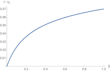
Figure 3: The time $t_{\rm sing}-t_{0}$, for the sudden singularity formation, is plotted in terms of the density $\bar{\rho}$.

III.2 Energy conditions

So far we have only obtained solutions to Eq. (5). In this section, we examine their compatibility with a set of energy conditions [42]. The “weak energy condition” is needed to be satisfied by standard matter. It guarantees, for example, the positiveness of the energy density for any local timelike observer. We need to define an effective energy density $\rho_{\rm eff}$ for the collapse to follow the energy conditions discussion according to their well-known form in GR.

Let us rewrite the modified Friedmann equation (5) in an effective relativistic form:

$$H^{2} = \frac{\kappa_{(4)}^{2}}{3}\rho_{\rm eff}-\frac{k}{a^{2}}\,,$$ (59)

where, we have introduced an effective energy density $\rho_{\rm eff}$ on the brane as

$$\rho_{\rm eff} := \rho+\frac{6\epsilon}{\kappa_{(5)}^{2}}\left(1+\frac{8}{3}\alpha h^{2}\right)h\,.$$ (60)

We introduce an effective pressure by defining an effective equation of state $w_{\rm eff}$ for a perfect fluid with an effective energy density $\rho_{\rm eff}$, as $p_{\rm eff}:=w_{\rm eff}\,\rho_{\rm eff}$. Thereby, an effective conservation equation can be written as

$$\dot{\rho}_{\rm eff}+3H(1+w_{\rm eff})\rho_{\rm eff}=0.$$ (61)

Then, using Eq. (60) we obtain

$$\dot{\rho}_{\rm eff} := \dot{\rho}+\frac{6\epsilon}{\kappa_{(5)}^{2}}\left(1+8\alpha h^{2}\right)\dot{h}\,,$$ (62)

where $\dot{h}$ is given by Eq. (48). From Eqs. (61) and (62) the effective pressure can be written as

$$p_{\rm eff} = -\rho_{\rm eff}-\frac{\dot{\rho}}{3H}-\frac{2\epsilon}{\kappa_{(5)}^{2}H}\left(1+8\alpha h^{2}\right)\dot{h}$$ (63)

$$= -\rho_{\rm eff}+\frac{2r_{c}h\rho}{2r_{c}h-\epsilon(1+8\alpha h^{2})}\,,$$

where in the second term, we have used the conservation equation (46) for the dust fluid.

The effective energy-momentum tensor should satisfy the energy conditions (ECs)

$$\textrm{EC.1}:\quad\quad \rho_{\rm eff}\ =\ \rho+\frac{6\epsilon}{\kappa_{(5)}^{2}}\left(1+\frac{8}{3}\alpha h^{2}\right)h\geq 0,$$ (64a)

$$\textrm{EC.2}:\quad\quad \rho_{\rm eff}+p_{\rm eff}\ =\ \frac{2r_{c}h\rho}{2r_{c}h-\epsilon(1+8\alpha h^{2})}\geq 0\,.$$ (64b)

The above inequality can be rewritten in terms of dimensionless parameters as

$$\textrm{EC.1}:\quad\quad\quad\quad\bar{\rho}+\epsilon\left(b+\bar{h}^{2}\right)\bar{h}\geq 0,$$ (65a)

$$\textrm{EC.2}:\quad\quad\quad\quad\frac{2\bar{h}\bar{\rho}}{2\bar{h}-\epsilon(b+3\bar{h}^{2})}\geq 0\,.$$ (65b)

The first energy condition (EC.1) above can be written for each branch, respectively, as

$$\bar{h}^{3}+b\bar{h}-\bar{\rho}\leq 0\quad\quad\textrm{for the $(-)$ branch,}$$ (66)

$$\bar{h}^{3}+b\bar{h}+\bar{\rho}\geq 0\quad\quad\textrm{for the $(+)$ branch}.$$ (67)

From Eq. (9a) we observe that ${\bar{h}}^{3}+b\bar{h}-\bar{\rho}=-{\bar{h}}^{2}<0$, thus, the EC.1 for the $(-)$ branch (i.e., the first equation above) is satisfied. Likewise, Eq. (9b) indicates that ${\bar{h}}^{3}+b\bar{h}+\bar{\rho}={\bar{h}}^{2}>0$, so the second inequality above [i.e., EC.1 for the $(+)$ branch] is also satisfied. Therefore, the EC.1 (65a) is respected in the herein effective theory for both branches.

The second energy condition (EC.2), given by (65b), can be written equivalently as

$$\textrm{EC.2a}\colon\quad\quad\bar{h}>0\quad\land\quad 2\bar{h}-\epsilon(b+3\bar{h}^{2})>0,\quad\quad\quad$$ (68a)

or

$$\textrm{EC.2b}\colon\quad\quad\bar{h}<0\quad\land\quad 2\bar{h}-\epsilon(b+3\bar{h}^{2})<0.\quad\quad\quad$$ (68b)

Depending on the sign of $\epsilon$ we can distinguish two different cases as we will analyze in the following.

III.2.1 The $(-)$ branch

In this case, one of the conditions EC.2a or EC.2b should be satisfied.

1. If the condition EC.2a, given by Eq. (68a), holds, we would have

   $$\quad\left\{\bar{h}>0\right\}\ \land\ \left\{\bar{h}<\bar{\mathfrak{h}}_{-}^{(1)}\ \lor\ \bar{h}>\bar{\mathfrak{h}}_{+}^{(1)}\right\},$$ (69)

   where both quantities $\bar{\mathfrak{h}}_{\pm}^{(1)}$ are negative and defined in Eq. (53). The intersection of the above sets reads $\bar{h}>0$, which means that the range of quantities $\bar{h}$ that holds EC.2a is $\bar{h}>0$. This condition results in a class of physically relevant solutions,

   $$\quad\textrm{EC.2a}\quad\Leftrightarrow\quad\left\{\bar{h}_{1}(\eta),\ \bar{h}_{4}(\theta),\ \bar{h}_{5},\ \bar{h}_{6}(\vartheta)\right\},\quad$$ (70)

   for the herein DGP-GB model of dust collapse (cf. Sec. II). In this case, $\bar{h}(t)$ is positive, having a lower bound at $\bar{k}/a(t)$ at any time $t$. But, it has no upper limit, so it can diverge at some time in the future.

2. The condition EC.2b in Eq. (68b) implies that

   $$\quad\left\{\bar{h}<0\right\}\ \land\ \left\{\bar{\mathfrak{h}}_{-}^{(1)}<\bar{h}<\bar{\mathfrak{h}}_{+}^{(1)}\right\}.$$

   Since $\bar{\mathfrak{h}}_{-}^{(1)},\,\bar{\mathfrak{h}}_{+}^{(1)}<0$, the intersection of two ranges above will be $\bar{\mathfrak{h}}_{-}^{(1)}<\bar{h}<\bar{\mathfrak{h}}_{+}^{(1)}$. In this range for $\bar{h}$, there exists only one physically reasonable solution,

   $$\textrm{EC.2b}\quad\Leftrightarrow\quad\bar{h}_{2}(\theta)\,.$$ (71)

The sets of solutions (70) and (71) display two separate scenarios: The first one (cf. EC.2a) represents a collapse starting from an initial configuration at some values $\bar{h}_{0}>0$ and evolving by increasing $\bar{h}_{2}(\theta)$ toward the $R=0$, at which $\bar{H}$, $\bar{\rho}$, and $\dot{\bar{H}}$ diverge. Therefore, the collapse end state in this case is a SFS. The second scenario (cf. EC.2b) performs a collapse starting from an initial state with $\bar{\mathfrak{h}}_{-}^{(1)}\leq\bar{h}_{0}<\bar{\mathfrak{h}}_{+}^{(1)}$ and evolves toward $\bar{\mathfrak{h}}_{-}^{(1)}$ by (negatively) decreasing function $\bar{h}(\theta)$. When it reaches $\bar{\mathfrak{h}}_{-}^{(1)}~{}(=\bar{h}_{A})$, the brane hits a SCS.

III.2.2 The $(+)$ branch

For this branch, we also have two cases, depending on if either of the conditions EC.2a or EC.2b is satisfied.

1. Following the condition EC.2a, two inequalities yield the condition on $\bar{h}$ as

   $$\left\{\bar{h}>0\right\}\ \land\ \left\{\bar{\mathfrak{h}}_{+}^{(2)}<\bar{h}<\bar{\mathfrak{h}}_{-}^{(2)}\right\},$$

   where $\bar{\mathfrak{h}}_{\pm}^{(2)}$ are both positive numbers given by Eq. (53). The intersection of two ranges above gives a physical range for the evolution of $\bar{h}$ as

   $$\bar{\mathfrak{h}}_{+}^{(2)}<\bar{h}<\bar{\mathfrak{h}}_{-}^{(2)}\,.\quad$$ (72)

   This positive range of $\bar{h}$ contains only one solution (cf. Table 1):

   $$\textrm{EC.2a}\quad\Leftrightarrow\quad\bar{\mathpzc{h}}_{2}(\theta).$$ (73)

2. Likewise, for the condition EC.2b, we get

   $$\left\{\bar{h}<0\right\}\ \land\ \left\{\bar{h}<\bar{\mathfrak{h}}_{+}^{(2)}\ \lor\ \bar{h}>\bar{\mathfrak{h}}_{-}^{(2)}\right\}.$$ (74)

   The intersection of the above sets provides a range of changes for $\bar{h}$ as

   $$\bar{h}<0\,.\quad$$ (75)

   This condition implies that the physically reasonable solutions for the $(+)$ branch in this case is given by the solutions (cf. Table 1):

   $$\textrm{EC.2b}\quad\Leftrightarrow\quad\left\{\bar{\mathpzc{h}}_{1}(\eta),\ \bar{\mathpzc{h}}_{4}(\theta),\ \bar{\mathpzc{h}}_{5},\ \bar{\mathpzc{h}}_{6}(\vartheta)\right\}.$$ (76)

The above argument describes two different scenarios for the herein collapse on the $(+)$ branch: The case EC.2a describes a collapse starting at an initial configuration with $\bar{h}_{0}$ holding the range $\bar{\mathfrak{h}}_{+}^{(2)}<\bar{h}_{0}<\bar{\mathfrak{h}}_{-}^{(2)}$ and then evolves by an incremental function $\bar{h}$ until it reaches the upper limit $\bar{\mathfrak{h}}_{-}^{(2)}=-\bar{h}_{A}^{\prime}$. In this limit, the brane ends up with a SCS. The second scenario, EC.2b, corresponds to a collapse that began from an initial state with $\bar{h}_{0}<0$ and evolves (by $\bar{h}$ decreasing negatively) toward the center. When it reaches $R=0$, the brane ends with a shell-focusing singularity.

As a consequence of the analysis we have presented in this section, we have found differences with respect to the scenarios provided by GR; therein, the energy densities always blueshift and eventually diverge, with the central shell-focusing (naked or black hole) singularities emerging. Instead, herewith our investigation within the DGP-GB modifications to the dynamics of the collapse, we have found a range for the parameter $b$ that leads to a different destiny for the collapse outcome. In particular, by choosing a convenient initial condition as $\rho_{0}<\rho_{A}$, $\dot{h}_{0}<0$ and for the range of parameter $0<b<\frac{1}{4}$, the collapse of a dust fluid on the DGP brane would terminate with a SCS abrupt event, rather different from the mere formation of a central singularity. In the next section, we will investigate the circumstances for the formation of black hole horizons.

IV Status of the black hole horizon

In this section, we will present the matching conditions at the boundary of the collapsing object on the brane with a convenient exterior geometry. We then apply such conditions to the particular solutions we retrieved for the herein DGP-GB collapse.

The modified Friedmann Eq. (59) can be written as

$$\dot{R}^{2}=f_{0}(R)+\epsilon f(R),$$ (77)

where, two functions $f_{0}(R)$ and $f(R)$ were introduced as

$$f_{0}(R) :=\frac{2Gm_{0}}{R}+\mathcal{E},\quad\quad$$ (78)

$$f(R) :=\frac{2Gm(R)}{R}\,=\,\left(\bar{h}^{3}+b\bar{h}\right)\frac{R^{2}}{b^{2}r_{c}^{2}}\,,$$ (79)

in terms of the physical radius $R$, where $\mathcal{E}\equiv-k\mathbf{r}_{\rm b}^{2}>-1$, and $m_{0}=(4\pi\mathbf{r}_{\rm b}^{3}a_{0}^{3}/3)\rho_{0}$ is the initial mass of the star. The first term in Eq. (79) stands for the pure relativistic effects, the second term stands for the DGP-GB modifications, and the term $\mathcal{E}$ is the energy per unit mass.

Since the OS collapse in GR is matched to a Schwarzschild exterior, our objective is to find a general static exterior geometry for our herein modified OS model. Let us then match the interior modified OS spacetime at the boundary $\Sigma$, to a convenient general, spherically symmetric static exterior metric of the form [26]

$$ds^{2}_{\rm ext}=-A^{2}(R)F(R)d\tau^{2}+F^{-1}(R)dR^{2}+R^{2}d\Omega^{2}\,,$$ (80)

for some unknown function $A(R)$ and $F(R)$,

$$F(R):=1-\frac{2GM(R)}{R}\,.$$ (81)

These two functions should be determined by employing a convenient set of matching conditions. Thus, following the approach presented in [26], we get

$$\dot{R}^{2} = -F(R)+\tilde{\mathcal{E}},\quad\quad$$ (82)

where $\tilde{\mathcal{E}}$ is a constant. Contrasting Eqs. (77) and (82), we obtain

$$F(R)\,=\,\tilde{\mathcal{E}}-f_{0}(R)-\epsilon f(R).\quad\quad$$ (83)

Moreover, by choosing $\tilde{\mathcal{E}}=\mathcal{E}-1$, without loss of generality, we get

$$F(R)\,=\,1-\frac{2Gm_{0}}{R}-\epsilon\frac{2Gm(R)}{R}\,.$$ (84)

Using this, we can introduce a generalized mass $M(R)$ in terms of the Schwarzschild mass $m_{0}$ and the modifications induced by the DGP-GB effects as

$$M(R) = m_{0}+\epsilon\,m(R).$$ (85)

This relation states that, in the presence of the DGP-GB modifications to GR, provided by the correction term $m(R)=(R/2G)f(R)\neq 0$, the exterior solution deviates from the standard Schwarzschild geometry. However, for the particular case of $\alpha=0$, and in the limit of larger scales (when the distances are much larger than $r_{c}$), the action (1) reduces to the four-dimensional Einstein-Hilbert action and the Schwarzschild solution is restored for the exterior.

In what follows, we will analyze the possible exterior geometries and the status of horizon formation at the dust boundary in terms of the the interior collapse solutions we have derived in Sec. II). We start by assuming that the collapse is initially untrapped, that is, the parameters $m_{0},b,r_{c}$, and $R_{0}$ are such that $F(R)$ is initially positive,

$$F(R_{0})=1-\frac{2Gm_{0}}{R_{0}}-\epsilon f(R_{0})>0\,.$$ (86)

Then, as the collapse evolves, depending on the induced-gravity effects, $F(R)$ may or may not become zero or negative. The roots of the equation $F(R_{H})=0$ provides the location of the horizon $R_{H}$ of the final black hole. If such a root does not exist, then no black hole would form.

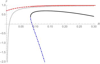
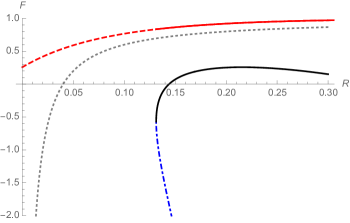
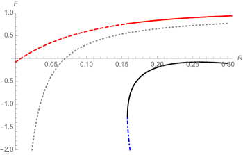
Figure 4: The evolution of the exterior functions associated with the interior solutions for $\epsilon=-1$ are depicted. The black and the red curves represent, respectively, exterior functions associated with the solutions $\bar{h}_{2}$ (leading to a SCS) and $\bar{h}_{4}$ (containing a SFS). The dashed blue and red curves depict the solutions $\bar{h}_{3}$ (physically irrelevant) and $\bar{h}_{1}$ (leading to SFS), respectively. Finally, the dotted gray curves are associated with the standard relativistic Schwarzschild geometry with $f_{0}(R)=1-2Gm_{0}/R$. The collapse parameters are chosen as $b=1/8$, $G=1$, $r_{c}=0.5$, and the initial values of the star mass are $m_{0}=0.005$ (upper), $m_{0}=0.02$ (middle), and $m_{0}=0.035$ (lower).

Figures 4 and 5 present numerical behaviors of the exterior function $F(R)$ for the physically relevant solutions we obtained in the Sec. II for the two branches, $\epsilon=\pm 1$. Both diagrams were plotted for the range of parameter $0<b<\frac{1}{4}$. In Fig. 4 the black and red curves depict the exterior functions associated with the two solutions $\bar{h}_{2}$ and $\bar{h}_{4}$, respectively. The dashed blue and red curves represent the exterior function corresponding to the solutions $\bar{h}_{3}$ and $\bar{h}_{1}$. Finally, the dashed gray curves depict the standard relativistic exterior function representing a Schwarzschild black hole geometry with constant mass $m_{0}$. On those figures, the points where the solid curves end and the dashed curves begin are the radii at the limiting regime $R_{A}$.

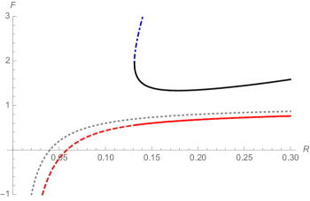
Figure 5: The evolution of the exterior functions associated with the interior solutions for $\epsilon=+1$ are depicted. The black curve represents the exterior function associated with the solution $\bar{\mathpzc{h}}_{2}$ (containing a SCS). The dashed and solid red curves depict the solutions $\bar{\mathpzc{h}}_{1}$ and $\bar{\mathpzc{h}}_{4}$ (containing SFSs), respectively. Finally, the dotted gray curve is associated with the standard relativistic Schwarzschild geometry with $f_{0}(R)=1-2Gm_{0}/R$. The collapse parameters are chosen as $b=1/8$, $G=1$, $r_{c}=0.5$, and $m_{0}=0.02$.

As it is shown in Fig. 4, for a set of initial parameters, there exist solutions in which the horizontal axis will not be crossed by $F(R)$, which indicates that no horizon would form in the collapse process and the final state of the collapse will be a naked SFS. To be more concrete, in Fig. 4 ($\epsilon=-1$ branch), the red solid curve represents the exterior function of a collapse that begins from a low energy regime [cf. the solution $\bar{h}_{4}$ in Eq. (36)] and evolves toward the limiting regime at $R_{A}$. Subsequently, it enters the high energy regime [governed by the solution $\bar{h}_{1}$, Eq. (19)] and proceeds toward the center. Depending on the choice of initial parameters, the exterior function may intersect the horizontal axis. If it reaches the horizontal axis, the final state for the exterior geometry will be a black hole. Likewise, for the solid black curve, there is a range of initial parameters for which, as the collapse proceeds from its initial condition up to the limiting regime at the radius $R_{A}$, no intersection between exterior function and the horizontal axis will happen; hence the exterior geometry will represent a naked sudden singularity. For other choices of the parameters, an apparent horizon would form and the final sudden singularity would be hidden by a black hole horizon.

Figure 5 depicts how the exterior geometry of the $(+)$ branch behaves differently. The exterior function associated with the interior solution $\bar{\mathpzc{h}}_{2}$ (which leads to a SCS) does not have an event horizon regardless of the initial mass $m_{0}$ value, thus the SCS is naked. On the other hand, the solutions $\bar{\mathpzc{h}}_{1}$ and $\bar{\mathpzc{h}}_{4}$, which result in SFSs, are always hidden inside the event horizon of a black hole.

V Conclusions and Outlook

In this paper, we investigated a higher-dimensional brane world extension of the general relativistic OS model for gravitational collapse. More precisely, we considered a DGP brane world model for gravitational collapse, where a GB term was present on the bulk. The brane was filled with a homogeneous dust fluid as matter content, whereas its geometry was governed by a closed FLRW metric.

From extracting the evolution equation of the brane, we subsequently provided a class of solutions relevant to describe a contracting brane. This conveys the gravitational collapse of a spherically symmetric object toward the central singularity.

We also obtained a particular solution in which, as the brane evolves toward a minimum nonzero radius, the energy density and $\bar{H}$ remain finite; the first time derivative of $\bar{H}$ diverges, though. Therefore, the brane reaches a particular singularity before it could reach the central singularity for which the energy density and the curvature of the brane become infinite. Such singularity is known as sudden singularity which would occur in a finite cosmic time in the future. Nevertheless, given that the singularity is reached in an infinite time from the point of view of an external observer, we will call it a sudden collapse singularity.

By employing a convenient matching condition at the boundary of the collapsing dust, we also provided an exterior solution for the collapse final state. By doing so, we were able to examine the role of the GB sector on the process and the outcome of the collapse. We have shown that for the $(+)$ branch, there exists a solution where the SCS happens before the formation of an event horizon. This occurs regardless of the initial conditions of the system. This is the direct consequence of the GB term which modifies the system in the high energy regime. The other shell-focusing solutions will have an event horizon no matter what initial settings they started with. On the other hand, in the case of the $(-)$ branch of the solution, the event horizon formation for the shell focusing depends on the initial conditions. Therefore, the SCS in this collapse scenario may not be accompanied by an event horizon.

The focus and scope of our paper herewith was to study the bound collapse $(k=1)$ on DGP-GB brane. The study of a marginal bound model $(k=0)$ was done in Ref. [28], which shows a similar result for the $(-)$ branch, in this sense that the formation of a naked or a black hole singularity depends on the initial condition. However, in the bound model $(k=1)$, the $(+)$ branch of the solutions does not violate the null energy condition in general, in contrast with the marginally bound system. Moreover, the $(+)$ branch in the bound collapse contains a characteristic solution that supports a naked SCS, which is independent of the initial condition.

Appendix A The cubic equation

In this appendix, we review very briefly a cubic equation representing the Friedmann equations (9a) or (9b) and their possible solutions following the prescription provided in Ref. [41].

Let us consider the general cubic equation:

$$z^{3}+a_{2}z^{2}+a_{1}z+a_{0}=0\ .$$ (87)

Let us define the variables as

$$Q = \frac{1}{3}\left(a_{1}-\frac{a_{2}^{2}}{3}\right),$$ (88)

$$S = \frac{1}{6}\left(a_{1}a_{2}-3a_{0}\right)-\frac{a_{2}^{3}}{27}\,,$$ (89)

and let us also introduce the discriminant function $N$ as

$$N=Q^{3}+S^{2}.$$ (90)

For $N>0$ there exists only one real root and a pair of complex conjugate roots; for $N=0$ there exists three real roots but at least two of them are equal; for $N<0$ there exists three real roots (irreducible case).

By defining the new variables

$$S_{1} = \left[S+\sqrt{N}\right]^{1/3},$$ (91)

$$S_{2} = \left[S-\sqrt{N}\right]^{1/3},$$ (92)

we can write the three solutions to the cubic equation (87) as

$$Z_{1} = (S_{1}+S_{2})-\frac{a_{2}}{3}\,,$$ (93a)

$$Z_{2} = -\frac{1}{2}(S_{1}+S_{2})-\frac{a_{2}}{3}+\frac{i\sqrt{3}}{2}(S_{1}-S_{2}),$$ (93b)

$$Z_{3} = -\frac{1}{2}(S_{1}+S_{2})-\frac{a_{2}}{3}-\frac{i\sqrt{3}}{2}(S_{1}-S_{2}).$$ (93c)

References

- Joshi [1987] P. S. Joshi, Global aspects in gravitation and cosmology (1987).
- Joshi [2012] P. S. Joshi, ed., Gravitational Collapse and Spacetime Singularities, Cambridge Monographs on Mathematical Physics (Cambridge University Press, 2012).
- Penrose [1969] R. Penrose, Gravitational collapse: The role of general relativity, Riv. Nuovo Cim. 1, 252 (1969), [Gen. Rel. Grav.34,1141(2002)].
- Deffayet [2001] C. Deffayet, Cosmology on a brane in Minkowski bulk, Phys. Lett. B502, 199 (2001), arXiv:hep-th/0010186 [hep-th] .
- Dvali et al. [2000] G. R. Dvali, G. Gabadadze, and M. Porrati, 4-D gravity on a brane in 5-D Minkowski space, Phys. Lett. B485, 208 (2000), arXiv:hep-th/0005016 [hep-th] .
- Cho and Neupane [2003] Y. M. Cho and I. P. Neupane, Warped brane-world compactification with Gauss-Bonnet term, Int. J. Mod. Phys. A18, 2703 (2003), arXiv:hep-th/0112227 [hep-th] .
- Randall and Sundrum [1999a] L. Randall and R. Sundrum, A Large mass hierarchy from a small extra dimension, Phys. Rev. Lett. 83, 3370 (1999a), arXiv:hep-ph/9905221 [hep-ph] .
- Randall and Sundrum [1999b] L. Randall and R. Sundrum, An Alternative to compactification, Phys. Rev. Lett. 83, 4690 (1999b), arXiv:hep-th/9906064 [hep-th] .
- Kofinas et al. [2003] G. Kofinas, R. Maartens, and E. Papantonopoulos, Brane cosmology with curvature corrections, JHEP 10, 066, arXiv:hep-th/0307138 [hep-th] .
- Deffayet et al. [2002] C. Deffayet, G. R. Dvali, and G. Gabadadze, Accelerated universe from gravity leaking to extra dimensions, Phys. Rev. D65, 044023 (2002), arXiv:astro-ph/0105068 [astro-ph] .
- Brown et al. [2005] R. A. Brown, R. Maartens, E. Papantonopoulos, and V. Zamarias, A late-accelerating universe with no dark energy- and a finite-temperature big bang, JCAP 0511, 008, arXiv:gr-qc/0508116 [gr-qc] .
- Bouhmadi-Lopez and Vargas Moniz [2008] M. Bouhmadi-Lopez and P. Vargas Moniz, Phantom-like behaviour in a brane-world model with curvature effects, Phys. Rev. D78, 084019 (2008), arXiv:0804.4484 [gr-qc] .
- Bouhmadi-Lopez et al. [2011] M. Bouhmadi-Lopez, A. Errahmani, and T. Ouali, The cosmology of an holographic induced gravity model with curvature effects, Phys. Rev. D84, 083508 (2011), arXiv:1104.1181 [astro-ph.CO] .
- Bouhmadi-Lopez et al. [2010] M. Bouhmadi-Lopez, Y. Tavakoli, and P. Vargas Moniz, Appeasing the Phantom Menace?, JCAP 1004, 016, arXiv:0911.1428 [gr-qc] .
- Charmousis and Dufaux [2002] C. Charmousis and J.-F. Dufaux, General Gauss-Bonnet brane cosmology, Class. Quant. Grav. 19, 4671 (2002), arXiv:hep-th/0202107 [hep-th] .
- Kim et al. [2000] J. E. Kim, B. Kyae, and H. M. Lee, Various modified solutions of the Randall-Sundrum model with the Gauss-Bonnet interaction, Nucl. Phys. B582, 296 (2000), [Erratum: Nucl. Phys.B591,587(2000)], arXiv:hep-th/0004005 [hep-th] .
- Nojiri et al. [2002] S. Nojiri, S. D. Odintsov, and S. Ogushi, Friedmann-Robertson-Walker brane cosmological equations from the five-dimensional bulk (A)dS black hole, Int. J. Mod. Phys. A17, 4809 (2002), arXiv:hep-th/0205187 [hep-th] .
- Davis [2003] S. C. Davis, Generalized Israel junction conditions for a Gauss-Bonnet brane world, Phys. Rev. D67, 024030 (2003), arXiv:hep-th/0208205 [hep-th] .
- Gravanis and Willison [2003] E. Gravanis and S. Willison, Israel conditions for the Gauss-Bonnet theory and the Friedmann equation on the brane universe, Phys. Lett. B562, 118 (2003), arXiv:hep-th/0209076 [hep-th] .
- Oppenheimer and Snyder [1939] J. R. Oppenheimer and H. Snyder, On Continued gravitational contraction, Phys. Rev. 56, 455 (1939).
- Tavakoli [2014] Y. Tavakoli, Astrophysical and cosmological doomsdays, Ph.D. thesis (2014), arXiv:1405.5455 [gr-qc] .
- Maeda [2006] H. Maeda, Final fate of spherically symmetric gravitational collapse of a dust cloud in Einstein-Gauss-Bonnet gravity, Phys. Rev. D73, 104004 (2006), arXiv:gr-qc/0602109 [gr-qc] .
- Jhingan and Ghosh [2010] S. Jhingan and S. G. Ghosh, Inhomogeneous dust collapse in D-5 Einstein-Gauss-Bonnet gravity, Phys. Rev. D81, 024010 (2010), arXiv:1002.3245 [gr-qc] .
- Tavakoli et al. [2017] Y. Tavakoli, C. Escamilla‐Rivera, and J. C. Fabris, The final state of gravitational collapse in Eddington‐inspired Born‐Infeld theory, Annalen Phys. 529, 1600415 (2017), arXiv:1512.05162 [gr-qc] .
- Ziaie and Tavakoli [2019] A. H. Ziaie and Y. Tavakoli, Gravitational collapse of Vaidya spacetime in Rastall theory of gravity, (2019), arXiv:1912.08890 [gr-qc] .
- Bruni et al. [2001] M. Bruni, C. Germani, and R. Maartens, Gravitational collapse on the brane, Phys. Rev. Lett. 87, 231302 (2001), arXiv:gr-qc/0108013 [gr-qc] .
- Gannouji [2018] R. Gannouji, DGP black holes on the brane, Eur. Phys. J. C78, 318 (2018), arXiv:1209.5128 [gr-qc] .
- Tavakoli et al. [2021] Y. Tavakoli, A. K. Ardabili, and P. Vargas Moniz, Exploring the cosmic censorship conjecture with a Gauss-Bonnet sector, Phys. Rev. D 103, 084039 (2021), arXiv:2012.05642 [gr-qc] .
- Bojowald et al. [2005] M. Bojowald, R. Goswami, R. Maartens, and P. Singh, A Black hole mass threshold from non-singular quantum gravitational collapse, Phys. Rev. Lett. 95, 091302 (2005), arXiv:gr-qc/0503041 [gr-qc] .
- Bojowald et al. [2008] M. Bojowald, T. Harada, and R. Tibrewala, Lemaitre-Tolman-Bondi collapse from the perspective of loop quantum gravity, Phys. Rev. D78, 064057 (2008), arXiv:0806.2593 [gr-qc] .
- Tippett and Husain [2011] B. K. Tippett and V. Husain, Gravitational collapse of quantum matter, Phys. Rev. D84, 104031 (2011), arXiv:1106.1118 [gr-qc] .
- Bambi et al. [2013] C. Bambi, D. Malafarina, and L. Modesto, Non-singular quantum-inspired gravitational collapse, Phys. Rev. D88, 044009 (2013), arXiv:1305.4790 [gr-qc] .
- Barcelo et al. [2008] C. Barcelo, S. Liberati, S. Sonego, and M. Visser, Fate of gravitational collapse in semiclassical gravity, Phys. Rev. D77, 044032 (2008), arXiv:0712.1130 [gr-qc] .
- Hajicek [1992] P. Hajicek, Quantum mechanics of gravitational collapse, Commun. Math. Phys. 150, 545 (1992).
- Marto et al. [2015] J. Marto, Y. Tavakoli, and P. Vargas Moniz, Improved dynamics and gravitational collapse of tachyon field coupled with a barotropic fluid, Int. J. Mod. Phys. D24, 1550025 (2015), arXiv:1308.4953 [gr-qc] .
- Tavakoli et al. [2014] Y. Tavakoli, J. Marto, and A. Dapor, Semiclassical dynamics of horizons in spherically symmetric collapse, Int. J. Mod. Phys. D23, 1450061 (2014), arXiv:1303.6157 [gr-qc] .
- Tavakoli et al. [2013] Y. Tavakoli, J. Marto, A. H. Ziaie, and P. Vargas Moniz, Semiclassical collapse with tachyon field and barotropic fluid, Phys. Rev. D87, 024042 (2013).
- Vaz and Witten [2001] C. Vaz and L. Witten, Quantum black holes from quantum collapse, Phys. Rev. D64, 084005 (2001), arXiv:gr-qc/0104017 [gr-qc] .
- Parvizi et al. [2021] A. Parvizi, T. Pawłowski, Y. Tavakoli, and J. Lewandowski, Rainbow Black Hole From Quantum Gravitational Collapse, (2021), arXiv:2110.03069 [gr-qc] .
- Barrow [2004] J. D. Barrow, Sudden future singularities, Class. Quant. Grav. 21, L79 (2004), arXiv:gr-qc/0403084 [gr-qc] .
- Abramowitz and Stegun [1965] M. Abramowitz and I. Stegun, Handbook of Mathematical Functions (Dover, 1965).
- Hawking and Ellis [2011] S. W. Hawking and G. F. R. Ellis, The Large Scale Structure of Space-Time (Cambridge University Press, 2011).