Influence of protostellar jets and HII regions on the formation and evolution of stellar clusters

Abstract

Context. Understanding the conditions in which stars and stellar clusters form is of great importance. In particular the role that stellar feedback may have is still hampered by large uncertainties.

Aims. We investigate the role played by ionising radiation and protostellar outflows during the formation and evolution of a stellar cluster. To self-consistently take into account gas accretion, we start with clumps of tens of parsecs in size.

Methods. Using an adaptive mesh refinement code, we run magneto-hydrodynamical numerical simulations aiming at describing the collapse of massive clumps with either no stellar feedback or taking into account ionising radiation and/or protostellar jets.

Results. Stellar feedback substantially modifies the protostellar cluster properties, in several ways. We confirm that protostellar outflows reduce the star formation rate by a factor of a few, although the outflows do not stop accretion and likely enough do not modify the final cluster mass. On the other hand, ionising radiation, once sufficiently massive stars have formed, efficiently expels the remaining gas and reduces the final cluster mass by a factor of several. We found that while HII radiation and jets barely change the distribution of high density gas, the latter increases, at a few places, the dense gas velocity dispersion again by a factor of several. As we are starting from a relatively large scale, we found that the clusters whose mass and size are respectively on the order of a few 1000 M_⊙ and a fraction of parsec, present a significant level of rotation. Moreover we found that the sink particles which mimic the stars themselves, tend to have rotation axis aligned with the cluster large scale rotation. Finally, computing the classical $Q$ parameter used to quantify stellar cluster structure, we infer that when jets are included in the calculation, the $Q$ values are typical of observations, while when protostellar jets are not included, the $Q$ values tend to be significantly lower. This is due to the presence of sub-clustering that is considerably reduced by the jets.

Conclusions. Both large scale gas accretion and stellar feedback, namely HII regions and protostellar jets, appear to significantly influence the formation and evolution of stellar clusters.

1 Introduction

It is largely established that a large fraction, and likely the majority, of stars forms in stellar clusters (Lada & Lada 2003; Bressert et al. 2010). As such, stellar clusters are certainly amongst the most important structures to understand in galaxies. This is particularly important to know the physical conditions that prevail as a star and its surrounding planets form and evolve.

How exactly stellar clusters form remains largely unknown and has been the subject of several recent reviews (Longmore et al. 2014; Krumholz et al. 2019; Krause et al. 2020; Adamo et al. 2020). While it is well established that their births take place through the collapse of massive gas proto-clusters, which likely have been observed (Urquhart et al. 2014; Elia et al. 2017), the exact conditions under which the collapse proceeds are still a matter of debate. Not only the initial conditions are still hampered by large uncertainties, in particular because gas clouds do not seem to present gas densities sufficiently high to reproduce the ones needed to explain the stellar densities in clusters (Krumholz et al. 2019) but also because the feedback effects and efficiency have still only been partially explored and quantified.

Starting from dense clumps, several authors have performed collapse calculations with various spatial resolutions ignoring stellar feedback (e.g. Bonnell et al. 2008; Bate 2012; Kuznetsova et al. 2015). In all these works, compact concentration of both gas and stars are naturally produced as a consequence of gravitational collapse. Lee & Hennebelle (2016a, b) closely investigated the radius of the gas proto-cluster as well as the stellar clusters and concluded that their mass-radius relation present similar scaling laws that the ones inferred from observations (e.g. Pfalzner et al. 2016). In this process, accretion-driven turbulence (Klessen & Hennebelle 2010) is playing a fundamental role. As gas falls in the gas proto-cluster, it sustains turbulent motion that get virialised and leads to the observed mass-size relation.

However it is firmly established that stellar feedback plays a fundamental role during the course of stellar cluster formation and evolution. The main stellar feedback processes believed to be significant by the time of the cluster formation are protostellar outflows, ionising radiation and stellar winds. The supernovae themselves arrive at least $4\text{\,}\mathrm{M}\mathrm{y}\mathrm{r}$ after the formation of the most massive stars and therefore likely do not play a significant role. Numerous studies have considered one or several feedback processes. This is particularly the case for ionising feedback which has been extensively studied (e.g. Dale et al. 2012, 2014; Walch et al. 2013; Geen et al. 2015, 2017; Gavagnin et al. 2017; Grudić & Hopkins 2019). There is a general agreement that the ionising radiation can efficiently disperse molecular clouds provide they are not bound, meaning that typically the escape velocity should not be larger than the sound speed of the ionised gas that is around $5\text{\,}\mathrm{k}\mathrm{m}{\scriptstyle.}\mathrm{s}^{-1}$. More precisely for molecular clouds typical of the solar neighbourhood, it has been inferred that the typical efficiency, that is to say the gas mass fraction which is converted into stars, is on the order of a few percents, although there are considerable variations. These variations are due on one hand to the stochastic nature of the gravo-turbulent fragmentation and on the other hand to the strong dependence of the ionising flux onto the stellar mass (Geen et al. 2018).

While several studies have considered the role of jets in cores (e.g. Offner & Chaban 2017) or low mass clusters (e.g. Cunningham et al. 2018), a somewhat more restricted numbers of studies have considered the role of jets at the scale of more massive clusters, that is to say a few parsecs across. For instance Nakamura & Li (2007) and Wang et al. (2010) considered star forming clumps of about $1000\text{\,}\mathrm{M_{\odot}}$ and show that turbulence can be maintained through the driving of jets but also that the star formation rate (SFR) can be reduced by a factor of a few compared to the case without jet driving leading to SFR that are typical of observed values. Guszejnov et al. (2021) explored the influence of jets on a large variety of clouds and also found that they have a significant influence on their evolution, particularly on the mass spectrum of the stellar objects. Similar results regarding the star formation efficiency (SFE) have been obtained using periodic boxes which in total also contain about $1000\text{\,}\mathrm{M_{\odot}}$ (Carroll et al. 2009; Federrath et al. 2014; Murray et al. 2018).

So far to our knowledge, no work have thus investigated the influence of both ionising radiation and protostellar outflows simultaneously. Moreover, most works that have included protostellar jets considered computational domain on the order of a few parsecs which makes the time both for accretion to proceed and jets to reach the computational domain a little short. Both aspects however are essential to assess the respective role of accretion driven turbulence and feedback driven turbulence. Indeed, protostellar outflows from stars in HII regions have been observed in our Galaxy, such as jets detected at the tip of dense gas pillars similar to the “Pillars of Creation” in M16 (McLeod et al. 2016).

In the present work, we aim at simulating the formation of a stellar cluster by describing self-consistently spatial scales from a few tens of pc down to about $1000\text{\,}\mathrm{a}\mathrm{u}$. This allows us to describe the proto-cluster environment while getting a reasonable description of the gaseous proto-cluster whose size ranges between 0.1 and $1\text{\,}\mathrm{p}\mathrm{c}$. We treat both ionising radiation and stellar jet feedback. By performing a series of simulations that include none, one or both feedback processes, we can induce their respective influence, in conjunction with large scale infall, on the gas and the stars.

The paper is organised as follows. The second part of the paper describes the numerical methods and the initial conditions of the runs performed. It is complemented by an appendix which describes in details our jet implementation. The third part of the paper presents the general description of the simulation results as well as a detailed analysis of the gas properties. It also discuss the star formation rate and efficiency obtained in the various simulations. The fourth part focuses on the gas properties with particular emphasis on the kinematic and the influence of the various types of feedback. The fifth part investigates the star/sink particle properties, namely the global rotation of the cluster, the stellar rotation axis orientation and the cluster structure, that we quantify using the $Q$ parameter. Section six concludes the paper.

2 Numerical methods and initial conditions

2.1 Code and numerical parameters

To investigate the joint influences of HII regions and protostellar jets on the formation of a stellar cluster, we carry out a set of four simulations starting from ${10}^{4}\text{\,}\mathrm{M_{\odot}}$ of gas in a cubic box of side $30.4\text{\,}\mathrm{p}\mathrm{c}$, differing only by the included type of stellar feedbacks. Thus, one simulation is including no feedback at all, one is including HII regions only, one is including protostellar jets only, and the last one is including both HII regions and protostellar jets.

These simulations have been made using $\mathcal{R}$amses (Teyssier 2002). This numerical Eulerian code uses Adaptative Mesh Refinement (AMR) technique to enhance resolution locally, where it is needed, on a Cartesian mesh. We use five levels of AMR, from 7 to 12. This gives a cell size of at least $0.24\text{\,}\mathrm{p}\mathrm{c}$ ($5\text{$\ {\scriptstyle.}$}{10}^{4}\text{\,}\mathrm{a}\mathrm{u}$) everywhere, and $7.4\text{$\ {\scriptstyle.}$}{10}^{-3}\text{\,}\mathrm{p}\mathrm{c}$ ($1.5\text{$\ {\scriptstyle.}$}{10}^{3}\text{\,}\mathrm{a}\mathrm{u}$) in the most refined cells. Our refinement criterion is based on Jeans length such that each local Jeans length is described by at least 40 cells.

We use open boundary conditions for the hydro solver to allow the matter to flow out of the box, and we use periodic boundaries for gravity. The refinement is not allowed in the outer 5% of the simulation box, to avoid the appearance of numerical instabilities in the matter flowing out of the box.

When the density in a cell rises above ${10}^{7}\text{\,}\mathrm{c}\mathrm{m}^{-3}$, we create a sink particle (Krumholz et al. 2004; Bleuler & Teyssier 2014) which interacts gravitationally with the surrounding gas and by the way of accretion and ejection processes. The radius and luminosity of the sinks are provided through evolutionary tables of Kuiper & Yorke (2013).

Our four simulations will include magnetic field. This latter is treated through the ideal magnetohydrodynamics approximation (Fromang et al. 2006). The cooling and heating processes are as described in Audit & Hennebelle (2005). It includes the most important atomic cooling and the heating photo-electric effect on PaH due to an external standard galactic UV field. Typically the resulting cooling curve is almost identical to the one obtained for instance in Koyama & Inutsuka (2000). This is in good agreement with earlier conclusions by Levrier et al. (2012) and Glover & Clark (2012) where comparisons between atomic and molecular cooling have been performed.

2.2 Stellar objects and ionising radiation

The resulting IMF in those simulations does not compare to the observed ones, partly due to a lack of numerical resolution but also to the fact that we do not treat here the infrared radiation that leads to a strong heating of the high density gas (Krumholz et al. 2007; Hennebelle et al. 2020). Indeed Lee & Hennebelle (2018b) found that when using an explicit barotropic equation of state to mimic the temperature at high density, a numerical resolution typically below 10 AU is needed to get numerical convergence on the stellar mass spectrum, in particular to describe the peak. This condition becomes even more severe, typically at least few AU of resolution are requested, when infrared radiation is treated (Hennebelle et al. 2020). While one may argue that not properly resolving the formation of low mass stars does not preclude to resolve the formation of high mass stars, the issue is that too many of the latter will then be produced because the total mass of gas converted in stars does not strongly depend on resolution. This issue may even be more severe when infrared radiation is treated since the resulting gas heating may then be overestimated and the number of massive stars further amplified.

Notably, the lack of massive stars in our simulations would be problematic for studying the influence of HII regions which are mainly triggered by massive stars. More generally the ionising flux emitted by massive stars strongly depend on their mass (e.g. Vacca et al. 1996). Even for a thousand solar masses in stars, the most massive star in our simulation hardly exceeds $10\text{\,}\mathrm{M_{\odot}}$ while observations suggest that statistically, for a pool of $120\text{\,}\mathrm{M_{\odot}}$ of stars, typically one massive star lies in them. To overcome this issue, we proceed as in Colling et al. (2018), where a simple sub-grid model is presented. Every time that $120\text{\,}\mathrm{M_{\odot}}$ of gas have been accreted into stars, we consider that one massive stars should have formed, so we create a stellar object whose mass is randomly chosen between 8 and $120\text{\,}\mathrm{M_{\odot}}$ assuming that the mass function is a power-law of index -2.35.

We do not use the approach in, e.g., He et al. (2019), where each sink particle is considered to be a core containing one massive star. This is a) because it is still unclear how much these cores should fragment into close binaries, which would change the distribution of massive stars in the cloud, and b) in order to allow a consistent set of stellar masses to be implemented in comparisons between simulations. The influence of the particular prescriptions made to introduce massive stars has been analysed in details by Grudić & Hopkins (2019), who concluded that it indeed results in large uncertainties, which can be as important as a factor of 3. Typically quantifying the influence of the prescriptions such as the random choices of the massive star masses (Geen et al. 2018) would require to perform several runs which is outside the scope of the present work. Along the same line, a statistical sample should also be run to quantify the influence of different random seeds of the initial turbulence, although this would increase the cost of the work even further.

Each stellar object emits an ionising radiation as given by Vacca et al. (1996). This ionises the surrounding gas, which then expands into a HII regions provided the strength of the radiative field compared to the density of the environment is sufficient, as described in Geen et al. (2015). The ionising radiation is treated using the RT method developed in Rosdahl et al. (2013) which treats the propagation of light using the reduced speed approximation (a factor of ${10}^{-4}\text{\,}$ is employed in this work as it is sufficient to capture the expansion of the ionisation front, provided it does not expand faster than $30\text{\,}\mathrm{k}\mathrm{m}{\scriptstyle.}\mathrm{s}^{-1}$ — a few times the speed of sound). As in Geen et al. (2015), we used 3 groups of photons to describe the ionisation of hydrogen and helium.

2.3 Implementation of protostellar jets

As our maximum resolution is of the order of a thousand astronomical units, we do not resolve all the physics responsible for the ejection of matter from young accreting stars known as protostellar jets. To still be able to take into account the effect of these jets on the large scale evolution, we implemented a sub-grid model based on the properties of the sink particles. Once a sink grows a mass higher than $0.15\text{\,}\mathrm{M_{\odot}}$, at each time step it expels $1/3$ of the mass accreted during this time step in the form of a circular biconic jet. The matter is expelled with a velocity equal to 24% of the escape velocity at the surface of the star. The direction of the ejection is given by the angular momentum of the sink. Each circular cone has an opening angle of $20^{\circ}$. The expelled material has the same specific thermal energy than the direct surrounding of the sink particle. Technical details of the implementation and references for the values above can be find in Appendix A.

2.4 Neglect of supernovae and stellar winds

Our work omits the influence of stellar winds and supernovae from massive stars. Simulations using a similar setup have explored the interaction between photoionisation feedback and winds (Dale et al. 2014; Geen et al. 2021; Lancaster et al. 2021b, c) or supernovae (Geen et al. 2016; Kimm et al. 2021). The reason for this is both scientific and technical. Except for large, long-lived cloud complexes, supernovae either occur too late or do not have sufficient compressive power to strongly influence either their host cloud or other nearby clouds (Seifried et al. 2018), although they are thought to be a trigger for new cloud formation (Inutsuka et al. 2015; Fujii et al. 2021).

Winds are more complex, since they are produced by stars during their main sequence, similarly to ionising radiation. Stellar winds shock the cloud material to very high temperatures ($>10^{6}\leavevmode\nobreak\$K, sufficient to emit x-rays, e.g. Guedel et al. 2008), which create hot bubbles that store large quantities of energy. Their low density means the bubbles themselves do not typically radiate energy strongly Mac Low & McCray (1988). However, strong cooling channels exist either through evaporation of dense structures in the cloud overrun by the wind bubble (Arthur 2012), or by turbulent mixing with the cloud material (Rosen et al. 2014; Lancaster et al. 2021a, see also Tan et al. 2021 for an analysis of turbulent mixing on shockfronts). In this case, wind bubbles become momentum-driven rather than pressure-driven (Silich & Tenorio-Tagle 2013), and their dyanmical influence drops considerably. In this mode, winds only significantly drive the expansion of HII regions at small radii (Geen et al. 2020; Olivier et al. 2021), similar to the influence of radiation pressure. However, they can still play a strong role in structuring the photoionised region around the star (Pellegrini et al. 2007; Rahner et al. 2017) or even trapping ionising radiation at early times (Geen & de Koter 2021). This has a non-linear influence on the evolution of HII regions that should be explored in more detail.

A more technical reason for omitting stellar winds is the relatively high computational cost in simulating them. The sound speed in photoionised gas is $\sim 10\leavevmode\nobreak\$km/s, compared to speeds sometimes exceeding 3000  km/s for stellar winds (Vink et al. 2011; Ekström et al. 2012). The Courant condition for gas flows on the simulation grid thus requires around 100 times more timesteps if winds or other sources of hot gas such as supernovae are included. We thus justify omitting them both because their influence is more subtle and requires additional research to determine when they are important, but also because to do so would drastically increase our computational costs and thus limit our ability to explore the core physics in this work.

2.5 Initial conditions

Our four simulations have the same initial conditions as they only differ by the types of stellar feedbacks included. Those initial conditions are very similar to those used by Lee & Hennebelle (2016a). To set the density, we divide the box into 3 concentric regions. The inner one is a Bonnor-Ebert-like spherical cloud whose diameter is $15.2\text{\,}\mathrm{p}\mathrm{c}$, half of the box length. In this inner cloud the number density $n$ is distributed according to a top hat function:

$$n\left(r\right)=\frac{n_{0}}{1+\left(\frac{r}{r_{0}}\right)^{2}}$$ (1)

with $r$ the distance of the cell from the centre of the box, $n_{0}=$8\text{$\ {\scriptstyle.}$}{10}^{2}\text{\,}\mathrm{c}\mathrm{m}^{-3}$$, and $r_{0}=$2.5\text{\,}\mathrm{p}\mathrm{c}$$. This lead to a mass of ${10}^{4}\text{\,}\mathrm{M_{\odot}}$ in this central region. The second region, beginning at the cloud edge, is a ring whose outer diameter is equal to the box length. The density in this ring is constant and equal to about $8\text{\,}\mathrm{c}\mathrm{m}^{-3}$, a tenth of the cloud edge density. The rest of the box, the eight corners, are filled with a constant density of $1\text{\,}\mathrm{c}\mathrm{m}^{-3}$.

The initial temperature set by the cooling function is about $10\text{\,}\mathrm{K}$ in the dense gas. We initialised the magnetic field with a uniform mass-to-flux ratio of about 8 in the $x$ direction.

To initialise the velocity we do not consider those three regions separately. We mimic roughly the turbulence of the interstellar medium by constructing a velocity field according to a probability distribution of the turbulence (see for example section 3 of Hennebelle & Falgarone 2012, for a review on turbulence in interstellar clouds): in Fourier space, the power spectrum of the velocity field follows a Kolmogorov turbulence law, and the phases are randomly chosen. This turbulent field is normalised to have a Mach number of 6.7.

Those initial conditions are set by specifying ratios of characteristic timescales in the inner regions of size $r_{0}$. We then define the free-fall time to sound-crossing time ratio $\tfrac{t_{\text{ff}}}{t_{\text{sc}}}=0.15$, the free-fall time to Alfvén-crossing time ratio $\tfrac{t_{\text{ff}}}{t_{\text{ac}}}=0.2$, and the free-fall time to turbulent-crossing time $\tfrac{t_{\text{ff}}}{t_{\text{tc}}}=1$. The two first ratios show that the thermal and magnetic support against gravity are low, while the turbulent support is the dominant one.

2.6 Runs performed

We used this numerical setup to run four simulations which differ only by the stellar feedback that is included. The first simulation – NF – is run without feedback at all. One simulation includes only protostellar jets as stellar feedback – PSJo – and another includes only HII regions – HIIRo. The last one – PSJ-HIIR – includes both protostellar jets and HII regions. The acronyms used to refer to those simulations are summarised in Table 1.

Simulation	No feedback	Jets only	HII regions only	Jets & HII regions
Protostellar jets	✗	✓	✗	✓
HII regions	✗	✗	✓	✓
Acronym	NF	PSJo	HIIRo	PSJ-HIIR

Table 1: Summary of the four runs performed. The check marks and crosses indicate whether or not the protostellar jets or the HII regions are included in the simulations. The acronym for each simulation is given on the last line. These acronyms will be used all across the article.

We also ran two simulations with protostellar jets as the unique source of feedback but with different properties for the jets than in the PSJo simulation. The jets in the simulation “jets - wider” exhibit a wider ejection angle of $30^{\circ}$ while it is $20^{\circ}$ in PSJo. The jets in the simulation “jets - faster” are expelled with a velocity equal to 48% of the escape velocity of the sink, while it is 24% in PSJo.

3 General description, star formation rate and star formation efficiency

3.1 Global appearance of the emerging structures

We first look at the appearance of the emerging star clusters and surrounding gas on Fig. 1 and 2 for the four simulations. Figure 1 shows the emerging clusters at intermediate scales, whereas Fig. 2 shows them at large scales. The two first columns show column density along two different lines of sight, and the third column shows the mean velocity norm along the second line of sight, weighted by density. The overplotted red circles represent the sink particles. The four simulations are visualised at the same time of $3.5\text{\,}\mathrm{M}\mathrm{y}\mathrm{r}$. The first row exhibits the column densities of the simulation without feedback, NF, the second one those of the simulation with jets only, PSJo, the third one those of the simulation with HII regions only, HIIRo, and the last row exhibits the column density of the simulation with both protostellar jets and HII regions, PSJ-HIIR. The simulations that do not include HII regions are pretty similar, exhibiting a flattened cluster of stars, surrounding by spiralling gas with a disk-like shape. In the case of simulations with jets, the distribution of the gas is a bit more messy, due to the presence of jets. Those jets are visible in the third panel of the second row as high velocity components from either side of the cluster. On the other hand, the simulations that include HII regions have a qualitatively different appearance. The two simulations exhibit a distribution of the gas which is much more shredded, due to the expansion of HII regions, which is clearly visible from the velocity maps displayed in the third column of Fig. 1 and 2. The disk-like shape of the gas which was visible in the simulations without HII regions is no longer visible. However the star cluster also seems to be a bit flattened in these simulations.

In the case of the simulations without HII regions, this disk-like shape of the gas correlated to the flattened aspect of the star cluster seems to indicate that a preferred angular direction emerges as the cluster forms. This is not surprising, as Verliat et al. (2020) exposed a mechanism through which a protostellar disk naturally form around a protostar even in the absence of initial rotation. Angular momentum with respect to the cluster center, which is not the mass center of the system, is produced by inertial forces. The same mechanism can be invoked here to explain the formation of this rotating structure emerging from the gravitational collapse. Moreover Lee & Hennebelle (2016a) inferred that the clusters formed in their simulations without feedback indeed significantly rotate due to angular momentum inherited from the large scale collapse.

An evolutionary sequence of the cluster seen at small scales is visible on Fig. 3. The arrows attached to the sink particles represent their velocities in the plane perpendicular to the line of sight. At $2\text{\,}\mathrm{M}\mathrm{y}\mathrm{r}$, NF and HIIRo are very similar as the expansion of HII regions has not yet occurred. At this time, the simulations with jets — PSJo and PSJ-HIIR — are already more messy and also look both similar. As time progresses, the cluster in NF, PSJo and PSJ-HIIR becomes organised in the disk-like shape which seems to rotate. In HIIRo, the cluster has been completely depleted of gas, and its rotation is less obvious.

\begin{overpic}[width=144.39223pt]{cluster_cooling_nsink7_nojet_dens_y_11_271.pdf} \put(20.0,65.0){{\color[rgb]{1,1,1}\text{NF}}} \end{overpic}

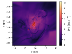
\begin{overpic}[width=144.39223pt]{cluster_cooling_nsink7_dens_y_11_329.pdf} \put(20.0,65.0){{\color[rgb]{1,1,1}\text{PSJo}}} \end{overpic}

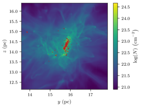
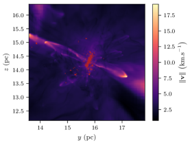
\begin{overpic}[width=144.39223pt]{cluster_cooling_nsink7_nojet_regionHii_dens_y_11_314.pdf} \put(20.0,65.0){{\color[rgb]{1,1,1}\text{HIIRo}}} \end{overpic}

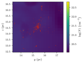
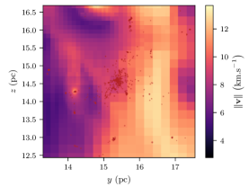
\begin{overpic}[width=144.39223pt]{cluster_cooling_nsink7_jet_regionHii_dens_y_11_373.pdf} \put(20.0,65.0){{\color[rgb]{1,1,1}\text{PSJ-HIIR}}} \end{overpic}

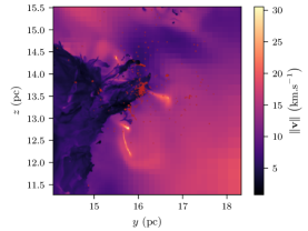
Figure 1: Global appearance of the star cluster surrounded by its gas environment. Each row corresponds to a different simulation. The four simulations are visualised at the same time of $3.5\text{\,}\mathrm{M}\mathrm{y}\mathrm{r}$. From top to bottom are the simulations without feedback, with protostellar jets only, with HII regions only, and with both jets and HII regions. The two first columns are column density along the $y$ and $x$ axis of the simulation, and the third column is the mean of the velocity norm integrated along the line of sight, weighted by the density. The colour scales are not common and depend on each map. The overplotted red circles represent the sink particles. As the view on the two last rows, corresponding to the simulations with HII regions, is a bit narrow, we presented on Fig. 2 the same maps with a spatial scale four times larger. We also present zooms on the central star cluster on Fig. 3.

\begin{overpic}[width=144.39223pt]{cluster_cooling_nsink7_nojet_dens_y_16_271.pdf} \put(20.0,65.0){{\color[rgb]{1,1,1}\text{NF}}} \end{overpic}

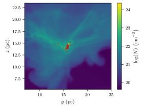
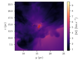
\begin{overpic}[width=144.39223pt]{cluster_cooling_nsink7_dens_y_16_329.pdf} \put(20.0,65.0){{\color[rgb]{1,1,1}\text{PSJo}}} \end{overpic}

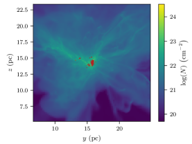
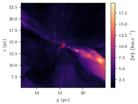
\begin{overpic}[width=144.39223pt]{cluster_cooling_nsink7_nojet_regionHii_dens_y_16_314.pdf} \put(20.0,65.0){{\color[rgb]{1,1,1}\text{HIIRo}}} \end{overpic}

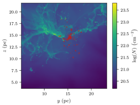
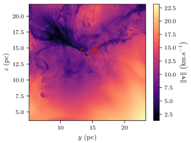
\begin{overpic}[width=144.39223pt]{cluster_cooling_nsink7_jet_regionHii_dens_y_16_373.pdf} \put(20.0,65.0){{\color[rgb]{1,1,1}\text{PSJ-HIIR}}} \end{overpic}

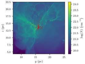
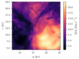
Figure 2: Global appearance of the star cluster surrounded by its gas environment, at a spatial scale four times larger than Fig. 1. The four simulations are visualised at the same time of $3.5\text{\,}\mathrm{M}\mathrm{y}\mathrm{r}$. Each row corresponds to a different simulation. From top to bottom are the simulations without feedback, with protostellar jets only, with HII regions only, and with both jets and HII regions. The two first columns are column density along the $y$ and $x$ axis of the simulation, and the third column is the mean of the velocity norm integrated along the line of sight, weighted by the density. The colour scales are not common and depend on each map. The overplotted red circles represent the sink particles.

\begin{overpic}[width=144.39223pt]{cluster_cooling_nsink7_nojet_dens_overplotsinkvel_y_18_154} \put(20.0,65.0){{\color[rgb]{1,1,1}\text{NF}}} \put(33.0,75.0){{\color[rgb]{0,0,0}$t=$2\text{\,}\mathrm{M}\mathrm{y}\mathrm{r}$$}}\end{overpic}

\begin{overpic}[width=144.39223pt]{cluster_cooling_nsink7_nojet_dens_overplotsinkvel_y_18_212} \put(33.0,75.0){{\color[rgb]{0,0,0}$t=$2.75\text{\,}\mathrm{M}\mathrm{y}\mathrm{r}$$}}\end{overpic}

\begin{overpic}[width=144.39223pt]{cluster_cooling_nsink7_nojet_dens_overplotsinkvel_y_18_271} \put(33.0,75.0){{\color[rgb]{0,0,0}$t=$3.5\text{\,}\mathrm{M}\mathrm{y}\mathrm{r}$$}}\end{overpic}

\begin{overpic}[width=144.39223pt]{cluster_cooling_nsink7_dens_overplotsinkvel_y_18_171} \put(20.0,65.0){{\color[rgb]{1,1,1}\text{PSJo}}} \end{overpic}

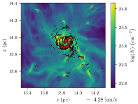
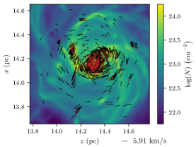
\begin{overpic}[width=144.39223pt]{cluster_cooling_nsink7_nojet_regionHii_dens_overplotsinkvel_y_18_154} \put(20.0,65.0){{\color[rgb]{1,1,1}\text{HIIRo}}} \end{overpic}

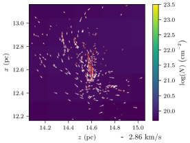
\begin{overpic}[width=144.39223pt]{cluster_cooling_nsink7_jet_regionHii_dens_overplotsinkvel_y_18_168} \put(20.0,65.0){{\color[rgb]{1,1,1}\text{PSJ-HIIR}}} \end{overpic}

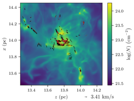
Figure 3: Evolutionary sequence of the global appearance of the star cluster. Each row corresponds to a different simulation. The four simulations are visualised at three different times, $2\text{\,}\mathrm{M}\mathrm{y}\mathrm{r}$, $2.75\text{\,}\mathrm{M}\mathrm{y}\mathrm{r}$ and $3.5\text{\,}\mathrm{M}\mathrm{y}\mathrm{r}$. From top to bottom are the simulations without feedback, with protostellar jets only, with HII regions only, and with both jets and HII regions, seen from the $y$ axis of the simulation. The colour scales are not common and depend on each map. The overplotted red circles represent the sink particles and the arrows associated represent their velocities in the plane of the visualisation.

3.2 Star formation rate and efficiency

The first and straightforward quantity to investigate is the total mass of the sink particles as a function of time. The slope of this curve represents the rapidity at which the stars accrete and is often refered to as the SFR while the final value of the accreted mass divided by the initial cloud mass represents the star formation efficiency (SFE).

The evolution of this total mass over time is presented on Fig. 4. The two orange curves represent the two simulations without HII regions, while the two purple ones represent the two simulations including HII regions. The two dashed lines represent the simulations without protostellar jets, while the two solid lines represent the simulations including them. The brown solid line and the yellow solid line represent the simulations with respectively wider and faster jets.

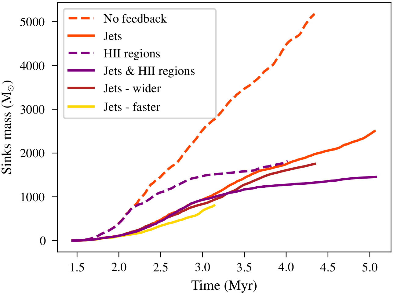
Figure 4: Total mass of the sink particles in the four simulations including or not different types of feedback. The two orange (respectively purple) curves stand for the simulations without (respectively with) HII regions. The dashed (respectively solid) lines represent the simulations without (respectively with) protostellar jets.

Let’s compare the two orange curves, thus the simulations without feedback at all on one hand, and with protostellar jets only on the other hand. After $2\text{\,}\mathrm{M}\mathrm{y}\mathrm{r}$ for the simulation without feedback, and $2.6\text{\,}\mathrm{M}\mathrm{y}\mathrm{r}$ for the simulations with jets, the total sink mass seems to evolve almost linearly with time. The SFR of these simulations is thus about $2\text{$\ {\scriptstyle.}$}{10}^{-3}\text{\,}\mathrm{M_{\odot}}{\scriptstyle.}\mathrm{y}\mathrm{r}^{-1}$ for the fisrt one, and about $8\text{$\ {\scriptstyle.}$}{10}^{-4}\text{\,}\mathrm{M_{\odot}}{\scriptstyle.}\mathrm{y}\mathrm{r}^{-1}$ for the second one. The difference in term of SFR when adding protostellar jets from a situation without feedback is thus a bit more than a factor two. This is consistent with what has been inferred previously in the litterature for instance by Wang et al. (2010) and Federrath et al. (2014) as can be respectivelly seen from Fig. 1 and 2 of these papers.

In Fig. 5, the orange dashdotted curve shows the ratio of the total sink mass in the simulation with protostellar jets over the total sink mass in the simulation without feedback : $M_{\text{sink,\text{PSJo}{}}}/M_{\text{sink,\text{NF}{}}}$. This curve exhibits a plateau for times larger than $2.6\text{\,}\mathrm{M}\mathrm{y}\mathrm{r}$, which corresponds to the linear regime of the orange curves in Fig. 4. The value of this plateau lies around 0.4, corresponding to the ratio $\frac{$8\text{$\ {\scriptstyle.}$}{10}^{-4}\text{\,}\mathrm{M_{\odot}}{\scriptstyle.}\mathrm{y}\mathrm{r}^{-1}$}{$2\text{$\ {\scriptstyle.}$}{10}^{-3}\text{\,}\mathrm{M_{\odot}}{\scriptstyle.}\mathrm{y}\mathrm{r}^{-1}$}$ of the two SFR. The orange dotted curve shows what this ratio would be if the difference in mass would only be due to the fraction of mass ejected in protostellar jets. This difference is easy to compute as the sub-grid model used for the protostellar jets specifies that each sink particle whose mass is larger than $0.15\text{\,}\mathrm{M_{\odot}}$ expels one third of the mass it accretes. In the limit of large times, the majority of the sink particles have a mass greatly larger than the mass threshold of $0.15\text{\,}\mathrm{M_{\odot}}$, thus the mass expelled by each sink tends toward the limit of $\frac{1}{3}$ of its accreted mass, leading to a ratio of $\frac{2}{3}$. We see that the ratio in the simulation is significantly lower than the one given by considering only ejected mass. This shows that an important effect of the protostellar jets is to diminish the accretion onto the sink particles. Thus the difference in mass is due to both the loss of the mass directly expelled by the jets and the reduction of the accretion rate onto the sink particles due to the interaction between the jets and the environment.

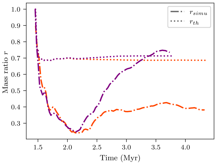
Figure 5: In dashdotted lines, $M_{\text{sink,\text{PSJo}{}}}/M_{\text{sink,\text{NF}{}}}$ in orange, and $M_{\text{sink,\text{PSJ-HIIR}{}}}/M_{\text{sink,\text{HIIRo}{}}}$ in purple. In dotted lines, the same ratios which would be obtained if the difference of total sink mass in those simulations would only be due to the fraction of mass ejected by protostellar jets.

The brown and yellow solid lines in Fig. 4 represent the two simulations with protostellar jets only but with different parameters for the jets than PSJo. The “jets - wider” uses wider jets while “jets - faster” uses faster jets. We see that the difference between these two curves and the orange solid one standing for PSJo is small compared to the influence of including or not the different types of feedback. All the analysis presented in the rest of this article were conducted for our six simulations. As the “jets - wider” and “jets - faster” simulations show similar results than PSJo for all the analysis, we will then ignore these two simulations for the remaining presentation.

Let’s now compare the four simulations NF, PSJo, HIIRo, PSJ-HIIR. In Fig. 4, we see that for times lower than $2.2\text{\,}\mathrm{M}\mathrm{y}\mathrm{r}$, the simulations without feedback at all, and with only HII regions behave strictly the same. This reflects the late onset of HII regions. The same observation can be made comparing the simulations with protostellar jets only, and with both protostellar jets and HII regions for times lower than $2.9\text{\,}\mathrm{M}\mathrm{y}\mathrm{r}$, with an onset of HII regions a bit delayed due to a lower SFR in the simulations including protostellar jets. Once the HII regions begin to have an impact on its parent cloud, the behaviour of the sinks mass starts to be different as the expansion of the HII regions becomes more and more important with time and with the apparition of stellar objects. Thereby the SFR in the simulations including HII regions tends to be lower and lower with time, entirely stopping star formation within a few million years, while the SFR in the simulations without HII regions is roughly constant as the sinks mass is nearly linear with time. Figure 6 shows the sinks mass separately for the two simulations that include HII regions, with indicators for the moments of formation of stellar objects which give birth to HII regions. On these two panels, the mass sequence of the different stellar objects is the same as the seed chosen to initialise the random number generator is the same. This permits close comparison, in particular ensuring that the differences between the two simulations are not coming from the random draw on stellar objects mass (Geen et al. 2018). We see that the first five stellar objects to form are not so massive, between 20 and $40\text{\,}\mathrm{M_{\odot}}$. As the mass of those stellar objects remains limited, and since they are formed in a dense environment, the HII regions associated are not powerful enough to expand and have a significant impact on the cluster. This explains the strong similarity in the sinks mass versus time between the corresponding simulations without HII regions before $2.2\text{\,}\mathrm{M}\mathrm{y}\mathrm{r}$ for the ones without jets, and before $2.9\text{\,}\mathrm{M}\mathrm{y}\mathrm{r}$ for the ones with jets. This similarity is also observed qualitatively on the gas distribution. The sixth stellar object to form has a mass of $102.6\text{\,}\mathrm{M_{\odot}}$. This rather massive stars is associated to a photon flux of about ${10}^{50}\text{\,}\mathrm{s}^{-1}$ and is able to form a HII region powerful enough to expand in this dense medium. In fact, we see in the two panels of Fig. 6 a change in behaviour just after the formation of this massive stellar objects (the vertical yellow line). Before its formation the SFR is increasing over time, and just after its formation the SFR starts decreasing over time. The stellar objects that form later have less impact than the $102.6\text{\,}\mathrm{M_{\odot}}$ one, but still contribute to the decrease in SFR.

In Fig. 5, the purple dashdotted curve shows the ratio of the total sink mass in the simulation with protostellar jets and HII regions over the total sink mass in the simulation including only HII regions: $M_{\text{sink,\text{PSJ-HIIR}{}}}/M_{\text{sink,\text{HIIRo}{}}}$. Between 1.6 and $2.2\text{\,}\mathrm{M}\mathrm{y}\mathrm{r}$, this curve is below the dotted purple curve, which represents what this ratio would be if the difference in sinks mass would only be due to the fraction of mass ejected in protostellar jets. As stated previously for the simulations without HII regions, this shows that the difference in mass is due to both the loss of the mass directly expelled by the jets and the reduction of the accretion rate onto the sink particles due to the interaction between the jets and the environment. At $2.2\text{\,}\mathrm{M}\mathrm{y}\mathrm{r}$, the ratio begins to increase over time. This is due to the appearance of the first HII regions which does not occur at the same time for the two simulations. In fact, between 2.2 and $2.9\text{\,}\mathrm{M}\mathrm{y}\mathrm{r}$, in the simulation including HII regions only, the first HII regions began to appear, while in the simulation which includes protostellar jets and HII regions, the HII regions have not expanded yet. Here we are then comparing simulations which have different behaviour in this time interval, and thus this increase in the ratio is not relevant.

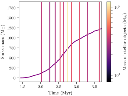
Figure 6: Left: total mass of the sink particles in the simulations including only HII regions. Right: total mass of the sink particles in the simulations including HII regions and protostellar jets. The purple curves in the two panels are thus corresponding to the same ones in Fig. 4. In the two panels, the vertical lines show the moments of creation of stellar objects, with the colours of the lines coding their mass.

In Appendix B we present the evolution of the number of sinks in time, for different masses of sinks. Figure 18 shows that for simulations with HII regions, the onset of HII regions stop most of the accretion onto the stars, while new small stars continue to form insensitively to the expansion of HII regions.

4 Gas density PDF and kinematic

In this section we investigate the gas properties focusing on the density PDF and the Mach number density relation within the whole computational box. We complement the analysis by studying the velocity dispersion of the dense structures.

4.1 Density PDF

\begin{overpic}[width=216.81pt]{pdf_rho_mult.pdf} \put(50.0,60.0){{\color[rgb]{0,0,0}\text{NF}{}}} \end{overpic}

\begin{overpic}[width=216.81pt]{pdf_rho_mult_bisjet.pdf} \put(50.0,60.0){{\color[rgb]{0,0,0}\text{PSJo}{}}} \end{overpic}

\begin{overpic}[width=216.81pt]{pdf_rho_mult_bisregionHii.pdf} \put(50.0,60.0){{\color[rgb]{0,0,0}\text{HIIRo}{}}} \end{overpic}

\begin{overpic}[width=216.81pt]{pdf_rho_mult_bis_jetregionHii.pdf} \put(50.0,60.0){{\color[rgb]{0,0,0}\text{PSJ-HIIR}{}}} \end{overpic}

Figure 7: Density PDF for the runs NF (top-left), PSJo (top-right), HIIRo (bottom-left) and PSJ-HIIR (bottom-right) for four snapshots (solid lines). The dotted lines visible in top-right and bottom left represent two snapshots of run NF, while the ones on bottom-right panel are from run HIIRo. The total accreted mass is indicated as it is more representative to make comparison between the runs.

The density PDF is a fundamental quantity to investigate not only because it reflects the dynamical state of the gas but also because it is believed to play a fundamental role regarding the mass spectrum of stars (Padoan et al. 1997; Hennebelle & Chabrier 2008; Lee & Hennebelle 2018a).

Figure 7 displays the density PDF for the four runs NF, PSJo, HIIRo and PSJ-HIIR for various snapshots. To make comparison easier, we have reported in the top-right panel (PSJo) and bottom-left one (HIIRo), two snapshots of run NF (dotted lines) using the color code to indicate what timesteps should be most comparable. In the bottom-right one (PSJ-HIIR), two snapshots of run HIIRo (dotted lines) have been reported.

The top-left panel portrays the density PDF of run NF. It is a clear powerlaw of index $\simeq-1.5$ typical of gravitational collapse arising in turbulent flows (Kritsuk et al. 2011; Lee & Hennebelle 2018a). The powerlaw is remarkably stable and does not evolve significantly over a period that goes from the cluster formation time up to the end of the simulation where about half of the gas has been accreted.

The top-right panel reveals that the jets have no significant influence on the density PDF, while the bottom-left panel shows that ionising radiation has a drastic role once massive enough stellar objects have formed. In particular, the quantity of gas at densities between ${10}^{2}\text{\,}$ and ${10}^{3}\text{\,}\mathrm{c}\mathrm{m}^{-3}$ is diminishing by one to two orders of magnitude compared to the case without feedback. On the contrary the quantity of gas at densities around $10\text{\,}\mathrm{c}\mathrm{m}^{-3}$ increases by almost one order of magnitude, which is a clear signature of the strong photo-ionisation that is induced by the massive stars. The bottom-right panel shows that even in the presence of ionising radiation feedback, the jets have very little influence on the density PDF. We note from both bottom panels that the high density gas is not strongly affected by the ionising radiation which is due to the recombination of electron and proton being very efficient at high densities.

4.2 Mach number density relation

\begin{overpic}[width=216.81pt]{pdf_mach_mult_bis_nojetnoregionHii.pdf} \put(40.0,18.0){{\color[rgb]{0,0,0}\text{NF}{}}} \end{overpic}

\begin{overpic}[width=216.81pt]{pdf_mach_mult_bisjet.pdf} \put(40.0,18.0){{\color[rgb]{0,0,0}\text{PSJo}{}}} \end{overpic}

\begin{overpic}[width=216.81pt]{pdf_mach_mult_bisregionHii.pdf} \put(40.0,18.0){{\color[rgb]{0,0,0}\text{HIIRo}{}}} \end{overpic}

\begin{overpic}[width=216.81pt]{pdf_mach_mult_bis_jetregionHii.pdf} \put(40.0,18.0){{\color[rgb]{0,0,0}\text{PSJ-HIIR}{}}} \end{overpic}

Figure 8: Same as Fig. 7 for the Mach-density relation.

A fundamental question with the feedback processes is how they exactly operate on the surrounding gas. For instance, do the jets increase the turbulence and by how much are crucial issues. Various teams (e.g. Carroll et al. 2009; Wang et al. 2010; Federrath et al. 2014; Offner & Chaban 2017; Murray et al. 2018) have all concluded that jets do trigger some turbulence although the importance of the effect vary between studies. This may be a consequence of the various setups that have been employed. Figure 8 displays the mean Mach number as a function of density for the four runs using the same conventions and snapshots than for Fig. 7.

The top-left panel shows that in the absence of feedback, the Mach number increases with density from about 1 to 30. It also increases with time for densities larger than $\sim${10}^{2}\text{\,}\mathrm{c}\mathrm{m}^{-3}$$. This is obviously a consequence of gravity which produces both infall and virial motions of the order of $\sqrt{GM/R}$, where $M$ is the accreted mass in the cluster and $R$ the typical distance from the cluster center.

The top-right panel reveals that the presence of jets increases the mean Mach number by tens of percents, mainly for intermediate densities of about ${10}^{3}\text{\,}\mathrm{c}\mathrm{m}^{-3}$, as visible when more than ${10}^{3}\text{\,}\mathrm{M_{\odot}}$ have been accreted. We therefore conclude that in the present configuration in which the turbulence is fed by accretion and in which the jet directions are not widely dispersed (see Sect. 5.4), turbulence is not strongly enhanced by the presence of jets. It is therefore likely that they mainly act by repulsing some of the gas that would have otherwise been accreted as indeed envisioned by Matzner & McKee (2000).

The importance of ionising radiation is visible from bottom panels. Clearly this feedback substancially modifies the mean Mach number at almost all densities. At about ${10}^{3}\text{\,}\mathrm{c}\mathrm{m}^{-3}$ it is on the order of 2 which implies a kinematic energy roughly four times larger and therefore influences much the gas behaviour. Note that the drop seen at ${10}^{2}\text{\,}\mathrm{c}\mathrm{m}^{-3}$ is due to the increase of the gas temperature. Let us stress that while the ionising radiation has little effect on gas temperature for densities above 10³ cm^-3 and below $\simeq$5 cm^-3, it can significantly heat, typically up to $T=$5000-8000 K, gas of intermediate densities. The presence of jets (bottom-right panel) further increases the Mach number for gas of densities ${10}^{3}\text{\,}\mathrm{c}\mathrm{m}^{-3}$ (compare blue dotted line and purple solid one), which is consistent with the final SFE being a bit lower when both jets and ionising radiation are included.

4.3 Dense structures internal velocity dispersion

\begin{overpic}[width=216.81pt]{CLUSTER_HOP_00250_10000.0_nojet__hist2D_mass_sig_250.pdf} \put(58.0,18.0){{\color[rgb]{0,0,0}\text{NF}{}}} \end{overpic}

\begin{overpic}[width=216.81pt]{CLUSTER_HOP_00300_10000.0_jet__hist2D_mass_sig_300.pdf} \put(58.0,18.0){{\color[rgb]{0,0,0}\text{PSJo}{}}} \end{overpic}

\begin{overpic}[width=216.81pt]{CLUSTER_HOP_00300_10000.0_nojethii__hist2D_mass_sig_300.pdf} \put(58.0,18.0){{\color[rgb]{0,0,0}\text{HIIRo}{}}} \end{overpic}

\begin{overpic}[width=216.81pt]{CLUSTER_HOP_00300_10000.0_jethii__hist2D_mass_sig_300.pdf} \put(58.0,18.0){{\color[rgb]{0,0,0}\text{PSJ-HIIR}{}}} \end{overpic}

Figure 9: Bidimensional histograms showing the velocity dispersion of dense structures for the four runs NF (top-left), PSJo (top-right), HIIRo (bottom-left) and PSJ-HIIR (bottom-right) at a time of about $3.2\text{\,}\mathrm{M}\mathrm{y}\mathrm{r}$.

Finally we complement the analysis presented in the previous section, which is a global estimate on the whole simulations, by investigating the local velocity dispersion of dense structures. The latter have been identified by running the HOP algorithm (Eisenstein & Hut 1998) on gas cells having densities larger than ${10}^{4}\text{\,}\mathrm{c}\mathrm{m}^{-3}$. While the mean Mach number analysis captures the large scale motions, which dominate in turbulent flows, the velocity dispersion of dense structures reveals the local motions in star forming clumps.

Figure 9 portrays the bidimensional histograms of the velocity dispersion of these structures at a time of about $3.2\text{\,}\mathrm{M}\mathrm{y}\mathrm{r}$. The top-left panel is typical of previous analysis reported in simulations without feedback (Hennebelle 2018; Ntormousi & Hennebelle 2019). Interestingly, top-right panel shows that in the presence of jets, the histogram presents a significant population of dense structures of gaseous masses between 0.1 and $1\text{\,}\mathrm{M_{\odot}}$ that have a velocity dispersion up to five times larger than the typical velocity dispersion $\left(\sim$0.3\text{\,}\mathrm{k}\mathrm{m}{\scriptstyle.}\mathrm{s}^{-1}$\right)$ found in the absence of jets. This indeed confirms that jets can locally perturb significantly the dense structures in which they develop. We note however that the bulk of the dense structures, that contains most of the mass, remains very similar to the one obtained in run NF.

The bottom panels show that ionising radiation has a moderate impact on the velocity dispersion of dense structures. The HIIRo run presents velocity dispersion slightly larger $\left(\text{say }\sim 50\%\right)$ than in run NF, while a similar, though even less pronounced, trend is observed between runs PSJo and PSJ-HIIR.

We conclude that altogether stellar feedback certainly alters the velocity dispersion and motions in star forming clumps by increasing it by a factor of a few (Goldbaum et al. 2011). However the nature of these motions cannot be simply described by a mere increase of turbulence. The net effect of the jets remains modest but they can have local very significant impact and this is probably why they reduce the SFR by a factor of roughly 2. On the contrary the ionising radiation appears to have even less impact on the dense gas but on the other hand they lead to global expansions — as visually obvious from Fig. 1 — that considerably decreases the SFE.

5 The stellar/sink properties

We now turn to the description of the stellar properties. We will then consider the sink particles as individual stars.

5.1 Bound and unbound stars

We saw in Fig. 3 that a lot of stars are forming around the central, dense cluster of stars in the simulations that include HII regions. In this part we try to distinguish between the stars bound to the cluster, and the ones that are destined to leave it.

We first compute bi-dimensional histograms of the sink positions and we took the bin of highest concentration as the cluster’s center. By doing it before and after the output of interest, we are also able to estimate the velocity of the cluster center. We then construct concentric spherical shells around the center. For each shell, we compute the escape velocity $V_{\text{esc}}$ at the shell radius $R$ as well as the mass, $M_{\text{int}}$, obtained by summing all the mass of sinks and gas at radii lower than $R$:

$$V_{\text{esc}}\left(R\right)=\sqrt{\frac{2GM_{\text{int}}}{R}}.$$ (2)

For each sink particle in the shell, we compute its projected velocity along the unit vector from the cluster’s center to the sink particle. This velocity is noted $V_{\text{rad}}$ and is positive if the sink particle is going away from the center and negative if going toward the center. In Fig. 10 we plotted all the sink particles in the four simulations with a color code indicating the ratio $\frac{V_{\text{rad}}}{V_{\text{esc}}}$. The sink particles in blue exhibit a ratio lower than 1, indicating that they should be bound at the time of interest. The ones in red exhibit on the contrary a ratio higher than 1. As they are moving away from the center at a speed higher than the escape velocity, they are destined to disperse and to leave the cluster, and we can consider these stars as unbound. We see that in the two upper panels representing simulations without HII regions (NF and PSJo), all the stars in the cluster are bound. For the two bottom panels, representing simulations with HII regions (HIIRo and PSJ-HIIR), the cluster consists of a bound core, surrounded by stars that are likely to disperse over time. The existence of unboud stars is likely to be due to the star formation in the material compressed by the expansion of HII regions. The escape velocity $V_{\text{esc}}$ is roughly constant over $R$, with a value about $2.4\text{\,}\mathrm{k}\mathrm{m}{\scriptstyle.}\mathrm{s}^{-1}$. The expansion of HII regions takes place at the sound speed in the ionized gas (Geen et al. 2015), which is about ten kilometres per second. A maximum value of about 4 for the ratio $\frac{V_{\text{rad}}}{V_{\text{esc}}}$ is coherent for stars that would have been formed in the expanding material of the HII regions.

\begin{overpic}[width=216.81pt]{cluster_cooling_nsink7_nojet_bound_y_271coq_min0.1ncoq20} \put(35.0,67.0){{\color[rgb]{0,0,0}\text{NF}{}}} \end{overpic}

\begin{overpic}[width=216.81pt]{cluster_cooling_nsink7_bound_y_329coq_min0.1ncoq20} \put(50.0,67.0){{\color[rgb]{0,0,0}\text{PSJo}{}}} \end{overpic}

\begin{overpic}[width=216.81pt]{cluster_cooling_nsink7_nojet_regionHii_bound_y_314coq_min0.1ncoq20} \put(26.0,67.0){{\color[rgb]{0,0,0}\text{HIIRo}{}}} \end{overpic}

\begin{overpic}[width=216.81pt]{cluster_cooling_nsink7_jet_regionHii_bound_y_373coq_min0.1ncoq20} \put(24.0,67.0){{\color[rgb]{0,0,0}\text{PSJ-HIIR}{}}} \end{overpic}

Figure 10: Distribution of stars in the four simulations at $3.5\text{\,}\mathrm{M}\mathrm{y}\mathrm{r}$. The colors code the ratio of the radial outward velocity of the sink particles over the escape velocity at their respective distance from the cluster’s center. Particles that appear in blue are likely to be bound, whereas the ones that appear in red are likely to be unbound.

5.2 Bound and unbound mass

We saw that in the two simulations that does not include HII regions, all the sinks are bound. This remains true for the entire temporal evolution. For the two simulations that include HII regions, namely HIIRo and PSJ-HIIR, they both exhibit unbound stars. Figure 11 shows the total amount of mass in bound and unbound stars in those two simulations. We see that in HIIRo the mass of unbound stars quickly grows to reach about a quarter of the total star mass. In PSJ-HIIR, the mass of unbound stars is three times lower, for the same mass of bound stars. As the evolution of the cluster in this simulation is slower, this indicates that the unbound stars form in the late stage, as HII regions are expanding in the outskirt of the cluster, triggering formation of unbound stars in these regions.

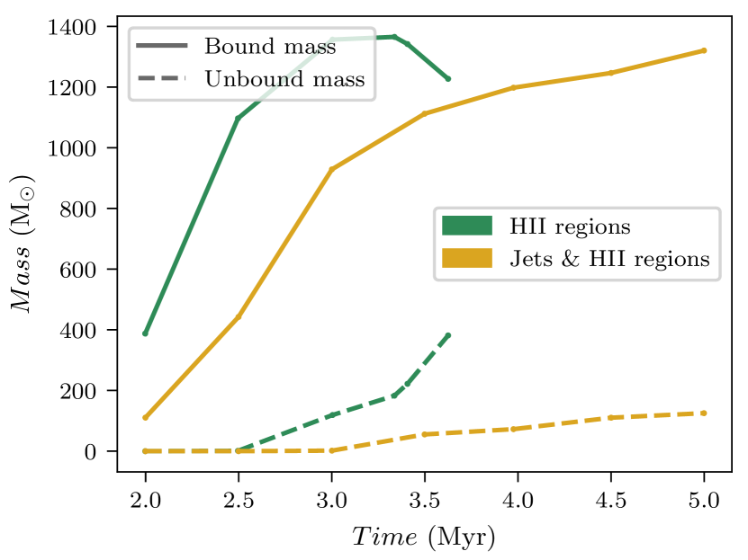
Figure 11: Evolution of the total mass of bound and unbound stars. The mass of unbound stars is significantly higher in the simulation HIIRo.

5.3 Rotation of the cluster

In this section we focus on the rotation of the bound part of the cluster. As in the previous section, we identify the cluster’s center as the place of highest concentration of stellar mass. We define the rotation axis of the cluster as the mean direction of the angular momentum of the bound sink particles. We define the equatorial plane as the plane perpendicular to the rotation axis and containing the cluster’s center. We then construct concentric cylindrical shells around the cluster center, aligned to the rotation axis. For each sink particle we compute the azimuthal velocity. We then divide the mean of the azimuthal velocities of the sink particles by the radius of the considered shell to obtain the mean angular velocity.

The profiles of the angular velocity is presented on Fig. 12. We see that for the simulations NF, PSJo and PSJ-HIIR, the angular velocity profiles are well defined and stable in time, except for early times (dark blue curves) when rotation seems not to be fully developed. They roughly follow a power-law of index -1.

The bottom left panel of Fig. 12 shows the angular velocity profiles for the simulation with HII regions only, HIIRo. Its velocity profiles show different behaviours compared to the ones of the other simulations. Note that the net rotation at $r\simeq$1\text{\,}\mathrm{p}\mathrm{c}$$ is nevertheless clear though a factor 2-3 lower than for the other runs. At $0.1\text{\,}\mathrm{p}\mathrm{c}$ they are lower by a factor of 10, whereas at $10\text{\,}\mathrm{p}\mathrm{c}$ they show similar values. They thus exhibit a flatter power-law. This behaviour could be due to the very early onset of the HII regions in this simulation, as shown by Fig. 4 and 6. This early onset could be responsible for a rapid emptying of the gas in the inner part of the cluster, disrupting the structure and preventing the stars from reaching the angular momentum corresponding to the profile observed in the other simulations. This does not happen in the simulation PSJ-HIIR which includes both HII regions and protostellar jets, as the jets slow down the accretion, allowing time for gas carrying large angular momentum to reach the cluster. This effect could be enhanced by the presence of unbound stars at late stages. At $3.5\text{\,}\mathrm{M}\mathrm{y}\mathrm{r}$, about a quarter of the mass of stars is unbound in HIIRo. These unbound stars could also play a role in perturbing the dynamics of the central bound stars.

Observationally, the situation appears to be complicated. Several authors (Hénault-Brunet et al. 2012; Kamann et al. 2018) report the presence of significant rotation on several clusters. Rotation velocities of a few $\text{\,}\mathrm{k}\mathrm{m}{\scriptstyle.}\mathrm{s}^{-1}$ are being measured and our simulations qualitatively agrees with this. However other observations (Kuhn et al. 2019) do not detect significant rotation in a sample of young stellar clusters. In our simulations, the presence of rotation is a clear consequence of the large scale collapse of a gaseous turbulent clump. If confirmed, the absence of rotation in a fraction of stellar clusters will probably require alternative scenario for stellar cluster formation.

\begin{overpic}[width=216.81pt]{cluster_cooling_nsink7_nojet_Multiple_omega_coq_min0.1ncoq20} \put(85.0,65.0){{\color[rgb]{0,0,0}\text{NF}{}}} \end{overpic}

\begin{overpic}[width=216.81pt]{cluster_cooling_nsink7_Multiple_omega_coq_min0.1ncoq20} \put(82.0,65.0){{\color[rgb]{0,0,0}\text{PSJo}{}}} \end{overpic}

\begin{overpic}[width=216.81pt]{cluster_cooling_nsink7_nojet_regionHii_Multiple_omega_coq_min0.1ncoq20} \put(80.0,65.0){{\color[rgb]{0,0,0}\text{HIIRo}{}}} \end{overpic}

\begin{overpic}[width=216.81pt]{cluster_cooling_nsink7_jet_regionHii_bis_smallr_Multiple_omega_coq_min0.1ncoq20} \put(75.0,65.0){{\color[rgb]{0,0,0}\text{PSJ-HIIR}{}}} \end{overpic}

Figure 12: Angular velocity profiles of the bound part of the cluster in the four simulations, at several times. The legend is shared by the four panels. Some of the profiles are missing in the two left panels since the corresponding simulations are not advanced enough.

5.4 Alignment of the stars in the cluster

As the clusters are rotating, we study here the alignment of the angular directions of the sink particles in our four simulations. Indeed spin alignment in two stellar clusters has been inferred by Corsaro et al. (2017), and by Kovacs (2018) in one cluster. We investigate whether or not a privileged direction also exists in the set of sink particles. An alignment is clearly expected in the simulations without HII regions as the gas exhibits a global rotating motion at the cluster scale. Then one may wonder what happens in the cases where HII regions are included. In particular, as the gas shows a lower global rotating motion, is the alignment still visible in the set of sink particles?

To answer these questions, we computed the mean direction of the sink particles angular momentum in each simulation, at each time step. The angular momentum of a sink particle is simply that of all the gas it has accreted. We then get the angular dispersion of the directions around this mean value by taking the standard deviation $\sigma_{\theta}$ of the angles between the sink directions and the mean direction previously computed. In order to be able to tell if the sinks are aligned with the mean direction, or on the contrary randomly distributed, we computed the same quantity $\sigma_{\theta}$ for a set with the same cardinality than the set of sink particles at each time step, exhibiting random angular orientations. The results over time for the four simulations are presented on Fig. 13. For times lower than $1.8\text{\,}\mathrm{M}\mathrm{y}\mathrm{r}$, the curves corresponding to the simulations and the ones corresponding to sets with random orientations are not distinguishable. At those times the sinks are not very massive, few in number, and the geometry of the gas flow is ill defined, which explains that we observe no particular alignment. However, after $1.8\text{\,}\mathrm{M}\mathrm{y}\mathrm{r}$, the angular dispersion begins to drop, stabilising at values between 20 and 40° for the four simulations. These values are lower than the ones corresponding to the sets of random orientations, which values tend to be constant and equal to about 50°. This shows that in those simulations the sink particles tend to align. This is expected from the gas geometry visible in the two first panels of Fig. 1, corresponding to the simulations without HII regions. In these two simulations the infalling gas forms a rotating disk-like structure around the star cluster, indicating a privileged direction as a global angular momentum emerges. In the two simulations which include HII regions, the sink particles also exhibit a preferred orientation. In Fig. 1 and 2 we see that the gas geometry is much more disorganised and dislocated than for the simulations without HII regions. Nevertheless, the sinks particles still exhibit a preferred orientation in these simulations which seems to survive through time as HII regions are developing. On the bottom panels of Fig. 14, the solid lines represent the same quantity than on Fig. 13, and we indicate the creation of the stellar objects with vertical coloured lines. In this first panel standing for the simulation with HII regions only, in solid green line, we see that after the formation of the most massive stellar object at $2.2\text{\,}\mathrm{M}\mathrm{y}\mathrm{r}$ the angular dispersion slightly increases gradually from 20° to around 33°. This increase could be due to the formation of unbound stars in the outskirt of the cluster as HII regions are expanding. Unlike central stars, unbound ones should not have a preferred direction as the dynamics of the gas is different at these places. In the second panel, representing the simulations with protostellar jets and HII regions, in solid yellow line, we see that there is no clear correlation between the slight variations of the angular dispersion and the onset of HII regions. It is thus unclear whether or not the HII regions play a role in modifying the angular dispersion here. A correlation is found only in the simulation with HII regions only. Moreover, even if the HII regions had an impact on this angular dispersion, it would be minimal as the variations in the other cases (and especially in the cases without HII regions) are of the same order of magnitude.

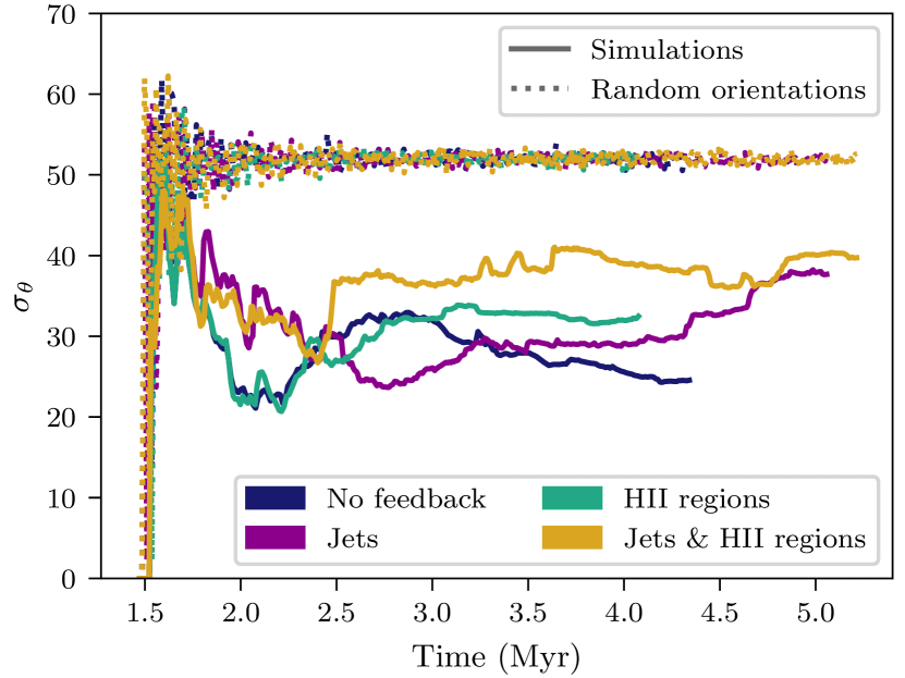
Figure 13: The solid lines show the angular dispersion of the sink particles relatively to the mean angular direction, each colour corresponding to a different simulation. To consider only relevant sink particles, we selected the ones with a mass larger than $0.07\text{\,}\mathrm{M_{\odot}}$. In comparison, the dotted lines show the angular dispersion of a set with the same cardinality than the set of sink particles at each time step, exhibiting random angular orientations. For times larger than $2\text{\,}\mathrm{M}\mathrm{y}\mathrm{r}$, the angular dispersion in the simulations is significantly lower than for a set of random orientations, implying that the sink particles have a preferred angular directions.

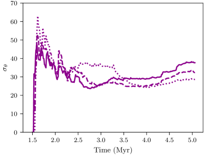
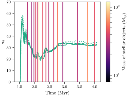
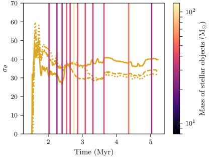
Figure 14: Angular dispersion of the sink particles distribution in each simulation. From top to bottom and from left to right are the simulations without feedback, with protostellar jets only, with HII regions only, and with both jets and HII regions. The different types of lines indicate the different mass sink thresholds used to define the sets. For the two simulations with HII regions, on the second row, we indicate the moments of creation of the stellar objects with vertical lines, whose colours code their mass.

The four panels of Fig. 14 represent the angular dispersion in the four simulations. The solid lines show the results for the same selection rule than in Fig. 13, which is that only sinks with a mass higher than $0.07\text{\,}\mathrm{M_{\odot}}$ are selected. The dashed and dotted lines show results for the sets of sink particles with a mass higher than $0.5\text{\,}\mathrm{M_{\odot}}$ and $1\text{\,}\mathrm{M_{\odot}}$ respectively. We see that for the first panel representing the NF simulation, the sets of higher masses exhibit slightly lower angular dispersion. This would mean that in this simulation the more massive stars are more aligned than the less massive ones. As the massive ones accrete more and more material from the oriented gas flow, they tend to align with time. When considering the less massive stars, as they are more sensitive to local slight variations in the gas flow, they exhibit a higher angular dispersion.

In the second panel and fourth panels, representing respectively the simulation PSJo and PSJ-HIIR, the sets of higher masses show higher angular dispersion during the first hundreds of kyrs of evolution, then the trend is reversing and the same behaviour than the one in NF is observed. A possible explanation for this behaviour could be that at the beginning of the formation of the cluster, sinks are not particularly aligned, as showed by Fig. 13. As time goes by, sinks are accreting matter. In NF, as a preferred orientation emerged from the gas flow, it is directly reflected in the sink particles behaviour. The massive ones are accreting more matter, and then are aligned more rapidly than the lower mass ones which are more sensitive to gas properties variations. In PSJo, the presence of jets modifies the accretion onto sink particles. The sink particles with a mass higher than $0.5\text{\,}\mathrm{M_{\odot}}$ have already started to launch protostellar jets. This modifies the direct environment of these sink particles, promoting accretion in their orthogonal plane, even if a global preferred orientation of the gas flow emerges. It is thus harder to change their initial orientation when the particles are accreting this way. The higher the mass of the particles, the more powerful the jets, and therefore the more impact they have on the direct environment of the particles. It is thus more difficult for the massive particles to align when protostellar jets are included. When considering lower mass particles with a threshold of $0.07\text{\,}\mathrm{M_{\odot}}$, we are taking into account all the newly formed particles, which are not affected by their own protostellar jets, thus are more sensitive to the gas flow geometry, and are directly formed with a preferred orientation on average as an orientation emerges in the flow. The angular dispersion in this set is thus lower here. At $3.5\text{\,}\mathrm{M}\mathrm{y}\mathrm{r}$ for PSJo and $2.9\text{\,}\mathrm{M}\mathrm{y}\mathrm{r}$ for PSJ-HIIR, the trend is reversing and the same behaviour than in NF is observed. As the massive particles are accreting more and more, they tend to align, even if the jets slow down this alignment, and we come back to a situation where the massive stars are the most aligned whereas the newly formed stars are more sensitive to variations and exhibit higher angular dispersion.

In the third panel, representing HIIRo, the three curves present similar trends and it is therefore hard to interpret the slight differences insofar as they could be due to the particular realisation. Furthermore, comparing NF and HIIRo in one hand – left panels –, and PSJo and PSJ-HIIR in the other hand – right panels –, we see that HII regions only have a minor influence on the observed behaviour, while protostellar jets seem to play a more important role in the alignment of the sink particles.

5.5 Spatial distribution of the emerging clusters

We now study the spatial distribution of the stars in the simulations, as traced by the sink particles. A first effect of feedback in the global cluster distribution can already be seen from visual inspection of previous figures in the text. All simulations start with a globally similar distribution of stars, as shown in the first column of Fig. 3. At later stages, however, it is clear from Fig. 2 (first column) or Fig. 10 (pay attention to spatial scales) that simulations with HII regions produce distributions with larger spatial dispersion, where the stars spread over a larger fraction of the region.

To globally characterise the distribution of stars and its evolution with time we computed the $Q$ parameter. This parameter, which has been introduced and developed by Cartwright & Whitworth (2004, 2009), has been widely used to objectively evaluate the level of sub-clustering or concentration in stellar clusters and associations. The value of $Q$ is given by the ratio of the mean distance of the members and the average length of their minimum spanning tree . Cartwright & Whitworth (2004) calibrated the $Q$ parameter in synthetic clusters and found that values of $Q>0.8$ correspond to radial concentration, $Q\simeq 0.8$ corresponds to clusters with homogeneous distribution, and $Q<0.8$ corresponds to clumpy clusters showing sub-clusterisation. To avoid over-interpretation in realistic distributions, these boundaries should not be strictly applied, and $Q$ should be used qualitatively. In appendix C we explain the details on the calculations performed in this work.

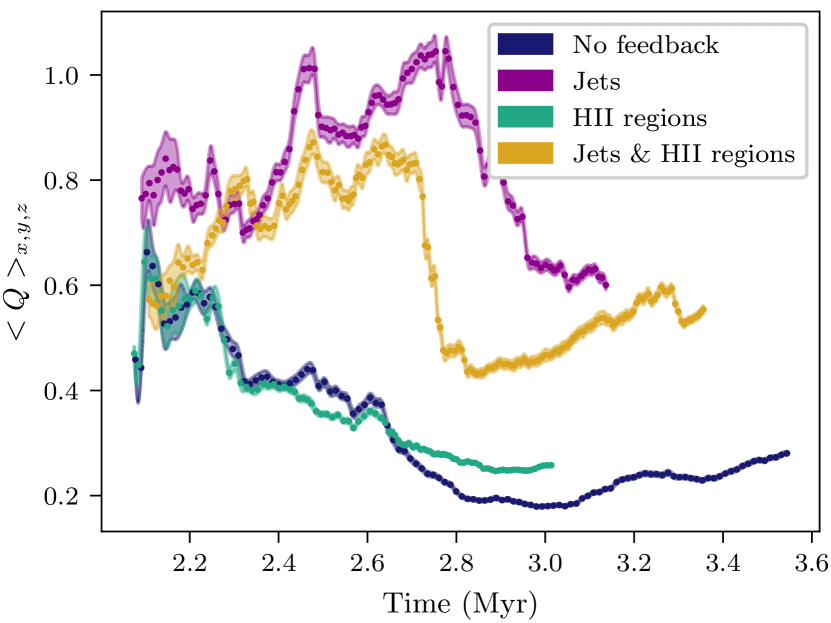
Figure 15: Evolution of the $Q$ parameter with time.

The evolution of $Q$ with time is shown in Fig. 15 where the $Q$ parameter is plotted over time for the four simulations represented by four distinct colours. The points represent the mean value of the $Q$ parameter, while the colour filled areas represent the interval of the mean value $\pm 1\sigma$. For each simulation, we begin at a time where approximately 300 sink particles are formed, in order to have enough sink particles in the sample.

The first notable result is that two clear trends appear. On one hand, the two simulations that include jets – PSJo and PSJ-HIIR – show a similar evolution over time, while in the other hand, the two simulations that do not include jets – NF and HIIRo – also show a similar trend, different from the first one.

Both PSJo and PSJ-HIIR show an increase in the $Q$ parameter between 2.1 to $2.7\text{\,}\mathrm{M}\mathrm{y}\mathrm{r}$, followed by a significant decrease. The initial increase in the $Q$ parameter indicates an evolution of the initial substructure presents in PSJ-HIIR, and an increase of the radial concentration in PSJo which, indeed, starts with $Q$ values around 0.8, consistent with homogeneous distributions. In both cases, the decrease in $Q$ around $2.7\text{\,}\mathrm{M}\mathrm{y}\mathrm{r}$ is associated to the growth of substructure in the outskirts of the field, far from the main cluster. These structures are small compared to the main clump of stars in the center, but the $Q$ parameter decreases as they become dense enough to be significant. The decrease is more abrupt in the simulation with an HII region, PSJ-HIIR, where a subsequent slow increase is also observed.

The two simulations without jets, NF and HIIRo, both show clear substructure at $2.1\text{\,}\mathrm{M}\mathrm{y}\mathrm{r}$ with a $Q$ parameter of about 0.6, that slowly and steadily decreases to 0.2 at $2.8\text{\,}\mathrm{M}\mathrm{y}\mathrm{r}$. At $3\text{\,}\mathrm{M}\mathrm{y}\mathrm{r}$, the $Q$ in NF slowly increases from 0.2 to 0.3 at $3.6\text{\,}\mathrm{M}\mathrm{y}\mathrm{r}$. These values of $Q\lesssim 0.3$ are much lower than the observed values for sub-clustered distributions and even that the box-fractal models in which the method was originally calibrated. In order to understand these very low values, we computed the $Q$ parameter of the inner part of the cluster, containing $90\%$ of the stars mass. This selection thus excludes the small substructures that grows far away from the central cluster. The $Q$ evolution is visible on Fig. 16 for this inner part, in the two simulations without HII regions – NF and PSJo. We see that the inner part in NF (blue dashed curve) exhibits higher and more stable values, between 0.4 and 0.7. This means that the very low values of the $Q$ parameter for the entire cluster is largely affected by the presence of sub-clusterisation in the outskirts. We also see that in the simulation PSJo (purple dashed curve), the drop at $2.7\text{\,}\mathrm{M}\mathrm{y}\mathrm{r}$ disappears, which confirms that this drop is associated to the growth of substructures in the outskirts of the field. Comparing the inner parts of NF and PSJo, we find that rapidly the $Q$ of PSJo rises over the one of NF. From $2.5\text{\,}\mathrm{M}\mathrm{y}\mathrm{r}$, PSJo exhibits a homogeneous inner region with a $Q$ of the order of 0.8, whereas NF still exhibits sub-clusterisation in its inner part, with a $Q$ between 0.45 and 0.7. We conclude that the protostellar jets seem to be efficient at preventing (or at least delaying) the apparition of substructures in the outskirts. Broadly speaking, the $Q$ values inferred in the presence of jets, appear in better agreement with the observations that when jets are absent.

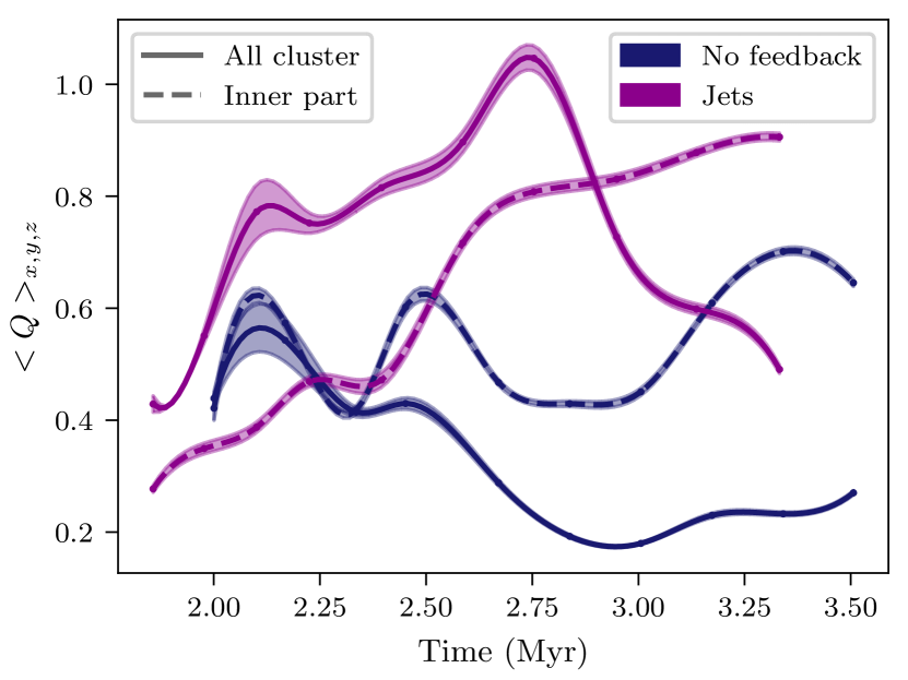
Figure 16: Smoothed temporal evolution of the $Q$ parameter for the entire cluster and for the inner part only, in NF and PSJo.

Our results show that protostellar jets seem to play an important role in the structuring and distribution of stars in the cluster, while HII regions, despite producing more disperse distributions, do not seem to produce statistically significant structural changes. Looking at the results presented in sections 4 and 5, jets and HII regions have different impacts on the gas and the star cluster. Protostellar jets only have a minor influence on the gas appearance while having a major influence on the stars distribution in the cluster. Conversely, HII regions have a major role in shaping the gas but their impact on the distribution of stars in the cluster is limited.

6 Conclusions and perspectives

6.1 Conclusions

To study the formation and evolution of stellar clusters, we performed a set a four simulations including or not the effects of HII regions and protostellar jets. We started from a turbulent, magnetised cloud of ${10}^{4}\text{\,}\mathrm{M_{\odot}}$ of gas.

The structures formed in these simulations have a very different appearance depending on whether or not HII regions are included. The expansion of the HII regions empties the central part and shreds the gas. We have shown that protostellar jets have a significant influence on the star formation rate. They slow down star formation, reducing the SFR by more than a factor of two, but do not stop star formation. The onset of HII regions also reduces the SFR but quickly leads to the dispersion of the gas in the cluster, which almost completely extinguishes the accretion onto stars and then decreasing the SFE.

The study of the gas reveals that the jets have almost no influence on the density distribution and have a moderate influence on the Mach number. On the contrary, the HII regions strongly alter the gas at intermediate densities and strongly modify the Mach number at all densities. It is thus difficult to find evidences for the presence of jets looking only at the kinematics of the gas. Turbulence in cluster forming clumps is primary due to gas accretion.

We then studied the emerging star clusters. In simulations without HII regions, all the stars formed are gravitationally bound. When HII regions are included, the cluster consists of a central core of bound stars surrounded by an outskirt of unbound stars. The clusters are rotating. We showed that the angular velocity profiles are stable in time. In the simulation with HII regions only, the early onset of HII regions could explain the low rotation of the cluster. We showed that the stars exhibit a preferred alignment of their own rotation axis. This alignment seems to persist through time, even in the simulation with HII regions only, where the global rotation of the cluster is less obvious. In order to characterise the spatial distribution of the formed stars, we calculated the $Q$ parameter of these clusters. Protostellar jets play a major role here. They seem to prevent the formation of sub-structures in the outskirt of the cluster. Simulation including protostellar jets thus showed distribution with less substructures, and the ones that still form appear in later times.

6.2 Perspectives

It would be interesting to further investigate the $Q$ parameter. One possibility could be to use the S2D2 algorithm developed by González et al. (2021) to detect significant small-scale sub-structures known as Nested Elementary STructures (NESTs). The study of these NESTs and their distribution could be a powerful way to interpret more precisely the $Q$ parameter of the emerging clusters.

One of the limitations of our study is the impossibility to run simulations with a significant statistics on the initial conditions, due to the high computational cost of this type of simulations. It would be valuable to run similar simulations with different initial conditions and different seeds for the random generator of the stellar object masses. As the expansion of HII regions is known to depend on the density of the gas where it takes place, varying the initial conditions would allow to investigate the statistics for the onset of HII regions.

One could also try to perform similar simulations with higher resolutions. It would then be possible to study the emerging initial mass function and to determine the individual and joint influences of HII regions and protostellar jets on it.

It would be interesting to investigate for longer times the mass fraction of bound and unbound stars and to follow those stars in time. In fact, it is known that some of the clusters are evaporating and Gavagnin et al. (2017) showed that cluster survival depends on feedback strength. Leading this study in simulations with different initial conditions would probably shed lights on conditions and processes responsible for the evaporation of such stellar clusters.

Appendix A Protostellar jets modelisation and implementation

In our simulations, the maximum resolution associated to the finest AMR level is about $1.5\text{$\ {\scriptstyle.}$}{10}^{3}\text{\,}\mathrm{a}\mathrm{u}$. This prevents to observe effects emerging from physical mechanisms happening at smaller scales. In particular we do not resolve all the physics responsible for the emission of protostellar jets. The theories describing these ejections of matter from young accreting stars such as the centrifugal acceleration mechanism or the X-wind model (see for example Federrath et al. 2014) involve physical mechanisms taking place on scales smaller than the astronomical unit. It is thus for the moment not possible to describe consistently the emission of protostellar jets and the dynamical formation of a star cluster in a $30.4\text{\,}\mathrm{p}\mathrm{c}$ simulation box.

A.1 The sub-grid model

To still be able to take into account the effect of these jets on the large scale evolution, we implement a sub-grid model based on the properties of the sinks. Once a sink grows a mass higher than $0.15\text{\,}\mathrm{M_{\odot}}$, at each timestep it expels $1/3$ of the mass accreted during this timestep in the form of a circular biconic jet. The matter is expelled with a velocity equal to a fraction $f_{v}$ of the escape velocity at the surface of the star. The direction of the ejection is given by the angular momentum of the sink. Each circular cone has an opening angle of $\theta_{\text{jet}}$. $f_{v}$ and $\theta_{\text{jet}}$ are fixed and are the same for all the sink particles in the simulation. Figure 17 shows a schematic view of the jets geometry around a sink particle.

Figure 17: Illustration of the geometric properties of the protostellar jets model. The central protostar is schematised is yellow, surrounded by its accretion disk in grey. The third of the accreted mass at each time step is ejected in a right circular bicone of opening angle $\theta_{\text{jet}}$ and of direction the angular momentum of the sink particle ${\@vec{j}_{\text{sink}}}$.

A.2 Implementation in $\mathcal{R}$amses

The numerical implementation of this sub-grid model of protostellar jets is made through a routine called just after the accretion onto the sinks. First of all, during a time step, the accretion of material onto each sink is processed. The mass accreted by each sink during this time step is stored in a variable which will be named here $m_{\text{acc},j}$ with the index $j$ referring to the sink number.

Once this accreted mass is computed, the routine setting protostellar jets is called. This routine contains a first loop over the CIC particles. Doing so, it is possible to identify the gas cells around each sink particle without having to scan the entire AMR grid. During this first loop, for each sink particle, the total volume of the cells that lay in a circular bicone around the sink is computed. A second loop over the CIC particles is done to redistributed some of the accreted quantities to the gas. For each sink particle, the quantities retrieved by each gas cell are proportional to the fraction of the cell volume over the total volume of gas cells in the circular bicone. This ensures that the quantity that is redistributed in the jet launch area is homogeneous over this area.

For each sink particle $j$ that exhibits mass greater than $0.15\text{\,}\mathrm{M_{\odot}}$, an arbitrary fraction $1/3$ of the accreted mass $m_{\text{acc},j}$ is given back to the gas cells. This value of $1/3$ is coherent with previous analytical, numerical, and observational studies of protostellar jets. For example, theories based on centrifugal acceleration or X-wind model by Blandford & Payne (1982); Pudritz & Norman (1986); Shu et al. (1988); Wardle & Koenigl (1993); Konigl & Pudritz (2000); Pudritz et al. (2007) and observations by Hartmann & Calvet (1995); Calvet (1998); Bacciotti et al. (2002); Cabrit et al. (2007); Bacciotti et al. (2011) suggest a fraction of the accreted mass which is ejected in the range of 0.1 to 0.4 (see page 4 of Federrath et al. 2014, for a review over these different studies and results). The arbitrary threshold of $0.15\text{\,}\mathrm{M_{\odot}}$ stands to ensure that the angular momentum of the sink particle is well defined when ejection begins. The velocity given to the ejected fraction of mass is equal to a fraction of the escape velocity at the protostar surface $v_{jet}=f_{v}\sqrt{2GM_{j}/R_{j}}$ with $M_{j}$ and $R_{j}$ being respectively the mass and radius of the protostar modelled by the sink particle. For $f_{v}$ between $0.25$ and $0.5$ this prescription gives jets velocities of the order of a hundred to a few hundreds of $\text{\,}\mathrm{k}\mathrm{m}{\scriptstyle.}\mathrm{s}^{-1}$. The matter deposited in the circular bicone is given an specific thermal energy which is the same than the one of the gas cell in which it is deposited.

Once these quantities are given back to the gas, they are deduced from the sink particles quantity: $M_{j}=M_{j}-\frac{m_{\text{acc},j}}{3}$. The linear and angular momentum, and the energy associated to each ejection is also calculated and subtracted from the linear and angular momentum of each sink particle.

Appendix B Evolution of the number of sinks

The evolution of the number of sinks with time is presented in Fig. 18. The four panels represent the four simulations. The y-axes have the same extent, but the x-axes extent depends on each panel. For the two simulations including HII regions, vertical lines indicate the formation of stellar objects.

We see that for the simulation including HII regions – HIIRo and PSJ-HIIR – the evolution of the number of sinks without using a mass threshold or using one of $0.07\text{\,}\mathrm{M_{\odot}}$ exhibits low influence of stellar objects formation. However, when we look at the sinks number using a mass threshold of $0.5\text{\,}\mathrm{M_{\odot}}$, we see that just after the apparition of the most massive stellar object (yellow vertical line), the increase in the number of stars shows a drastic drop. This is also the case for the stars with a mass higher than $1\text{\,}\mathrm{M_{\odot}}$ in HIIRo, but not in PSJ-HIIR where this change in behaviour is seen at $3.3\text{\,}\mathrm{M}\mathrm{y}\mathrm{r}$. This results show that stars continue to form in simulations with HII regions, but it is essentially low mass stars. HII regions seems to be efficient at cutting accretion onto the less massive stars as they form but do not accrete enough to grow higher masses when the HII regions are developing.

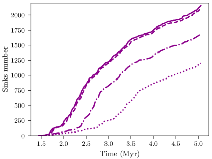
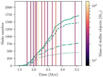
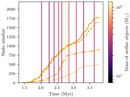
Figure 18: Evolution of the number of sinks during the temporal evolution. From top to bottom and from left to right, the simulation NF, PSJo, HIIRo, and PSJ-HIIR. For the simulations with HII regions, vertical lines indicate the formation of stellar objects, with the colours coding for their mass. In the four panels, the solid lines indicate the total number of sinks, the other types of line (dashed, dash-dotted, and dotted respectively) indicate the number of sinks with a mass lower than a threshold (0.07, 0.5 and $1\text{\,}\mathrm{M_{\odot}}$ respectively).

Appendix C $Q$ parameter

In this appendix we describe the specific calculations of $Q$ performed in this work, along with their motivation. We refer the reader to Appendix B in González et al. (2021) for a recent review on the $Q$ parameter method and its alternatives.

The $Q$ parameter is defined by:

$$Q=\frac{\bar{l}_{\text{MST}}}{\bar{s}}$$ (3)

where $\bar{s}$ is the normalized mean distance between stars, and $\bar{l}_{\text{MST}}$ is the normalized mean edge length of the minimum spanning tree (MST) (see e.g. Borůvka 1926; Kruskal 1956; Prim 1957; Gower & Ross 1969). A spanning tree is a set of straight lines connecting all the points of the sample without cycle. The MST is the unique spanning tree whose sum of edges is minimal. To allow for the comparison of regions of different size, the values of $\bar{s}$ and $\bar{l}_{\text{MST}}$ are normalised. Following Cartwright & Whitworth (2004), $\bar{s}$ should be normalised with a radius representative of the size of the cluster, and $\bar{l}_{\text{MST}}$ with a factor that includes the area subtended by the MST and the minimum number of points. We use consistent normalisation area $A$ for the MST and radius $R$ for the cluster, that follow the relationship $A=\pi R^{2}$.

Despite giving the boundary $Q=0.8$, there is some dispersion in the $Q$ values obtained in Cartwright & Whitworth (2004) that can be associated to sampling effects and the different random realisations of each distribution. This dispersion implies that even synthetic clusters with low degree of substructure or concentration are not statistically distinguishable from homogeneous.

As the $Q$ parameter has been introduced to describe observed clusters, $\bar{s}$ and $\bar{l}_{\text{MST}}$ were calibrated by Cartwright & Whitworth (2004) using the projected position of the stars in the plane of the sky for a set of synthetic clusters, with radial concentration, homogeneous distribution, or fractal sub-clusterisation. Despite the fact that in our simulations we have access to the 3D positions of the stars, we perform the calculations in projection, for consistency and to allow for comparisons with previous results. We compensate for the potential effects of projection onto a specific plane by calculating three 2D projections of each snapshot (using the $x$, $y$, and $z$ axis of the simulation as lines of sight) and averaging the obtained value of $Q$ of the three projections, $Q=\frac{1}{3}\left(Q_{x}+Q_{y}+Q_{z}\right)$ ,with its corresponding standard deviation $\sigma=\frac{1}{3}\sqrt{\sigma_{x}^{2}+\sigma_{y}^{2}+\sigma_{z}^{2}}$. We note that in any case, the projection effects are not severe, with globally similar results in the three projections.

The values of the $Q$ parameter can be sensitive to the presence of outliers, so we apply a resampling strategy to mitigate their effect. For each snapshot we randomly choose a subsample with 90% of the stars, compute the $Q$ parameter on this set, and repeat the process 100 times. This gives a distribution of the values of $Q$ within the sample, with its associated mean value and standard deviation.