Posterior Representations for Bayesian Context Trees:
Sampling, Estimation and Convergence

Abstract

We revisit the Bayesian Context Trees (BCT) modelling framework for discrete time series, which was recently found to be very effective in numerous tasks including model selection, estimation and prediction. A novel representation of the induced posterior distribution on model space is derived in terms of a simple branching process, and several consequences of this are explored in theory and in practice. First, it is shown that the branching process representation leads to a simple variable-dimensional Monte Carlo sampler for the joint posterior distribution on models and parameters, which can efficiently produce independent samples. This sampler is found to be more efficient than earlier MCMC samplers for the same tasks. Then, the branching process representation is used to establish the asymptotic consistency of the BCT posterior, including the derivation of an almost-sure convergence rate. Finally, an extensive study is carried out on the performance of the induced Bayesian entropy estimator. Its utility is illustrated through both simulation experiments and real-world applications, where it is found to outperform several state-of-the-art methods.

Keywords. Discrete time series, Bayesian context trees, branching processes, exact sampling, consistency, model selection, prediction, entropy estimation, context-tree weighting.

1 Introduction

The statistical modelling and analysis of discrete time series are important scientific and engineering tasks, with a very wide range of applications. Numerous Markovian model classes have been developed in connection with these and related problems, including mixture transition distribution (MTD) models (Raftery, 1985; Berchtold and Raftery, 2002), variable-length Markov chains (VLMC) (Bühlmann and Wyner, 1999; Bühlmann, 2000; Mächler and Bühlmann, 2004) and sparse Markov chains (Jääskinen et al., 2014; Xiong et al., 2016). Alternative approaches also include the use of multinomial logit or probit regression (Zeger and Liang, 1986), categorical regression models (Fokianos and Kedem, 2003), and conditional tensor factorisation (Sarkar and Dunson, 2016).

A popular and useful class of relevant models for discrete time series are the context-tree sources, introduced by Rissanen (1983a, b, 1986) as descriptions of variable-memory Markov chains, a flexible and rich class of chains that admit parsimonious representations. Their key feature is that the memory length of the chain is allowed to depend on the most recently observed symbols, providing a richer model class than ordinary Markov chains. Context-tree sources have been very successful in information-theoretic applications in connection with data compression (Weinberger et al., 1994; Willems et al., 1995), and the celebrated context tree weighting (CTW) algorithm (Willems et al., 1995; Willems, 1998), also based on context-tree sources, has been used widely as an efficient compression method with extensive theoretical guarantees and justifications.

Recently, Kontoyiannis et al. (2022) revisited context-tree models and the CTW algorithm from a Bayesian inference point of view. A general modelling framework, called Bayesian Context Trees (BCT), was developed for discrete time series, along with a collection of efficient algorithmic tools both for exact inference and for posterior sampling via Markov chain Monte Carlo (MCMC). The BCT methods were found to be very effective in important statistical tasks, including model selection, estimation, prediction and change-point detection (Papageorgiou et al., 2021; Lungu et al., 2022b, a); see also the R package BCT (Papageorgiou et al., 2020).

In this work we derive an alternative representation of the posterior distribution induced by the BCT framework, and explore several ways in which it facilitates inference, both in theory and in practice. Our first main contribution is described in Sections 3.1 and 3.2, where we show that both the prior and posterior distributions on model space admit explicit representations as simple branching processes. In particular, sampling tree models from the prior or the posterior is shown to be equivalent to generating trees via an appropriate Galton-Watson process (Athreya and Ney, 2004; Harris, 1963), stopped at a given depth. Therefore, in some sense the BCT model prior acts as a ‘conjugate’ prior for variable-memory Markov chains. An immediate first practical consequence of this representation is that it facilitates direct Monte Carlo (MC) sampling from the posterior, where independent and identically distributed (i.i.d.) samples can be efficiently obtained from the joint posterior distribution on models and parameters. This variable-dimensional sampler and its potential utility in a wide range of applications (including model selection, parameter estimation and Markov order estimation) are described in Section 3.3.

The Bayesian perspective adopted in this work is neither purely subjective nor purely objective. For example, we think of the model posterior distribution as a summary of the most accurate, data-driven representation of the regularities present in a given time series, but we also examine the frequentist properties of the resulting inferential procedures (Gelman et al., 1995; Chipman et al., 2001; Bernardo and Smith, 2009). Indeed, in Section 4 we employ the branching process representation to show that the posterior asymptotically almost surely concentrates on the “true” underlying model (Theorem 4.1), and in Theorem 4.2 we derive an explicit rate for this convergence as a function of the sample size. Analogous results are established in Theorems 4.3 and 4.4 in the case of out-of-class modelling, when the data are generated by a model outside the BCT class. Importantly, the limiting model is explicitly identified in this case. The branching process representation is also used in Proposition 4.1 to provide a simple, explicit representation of the posterior predictive distribution. These theoretical results are the second main contribution of this work.

Our last contribution, in Section 5, is a brief experimental evaluation of the utility of the MC sampler of Section 3, and a careful examination of the performance of the induced Bayesian entropy estimator. In Section 5.1, the new i.i.d. sampler is compared with the MCMC samplers introduced by Kontoyiannis et al. (2022) on simulated data. As expected, it is found that the i.i.d. sampler has superior performance, both in terms of estimation accuracy and, as expected, in terms of mixing.

Finally, in Section 5.2 we consider the important problem of estimating the entropy rate of a discrete time series. Starting with the original work of Shannon (1951), many different approaches have been developed for this task, including Lempel-Ziv (LZ) estimators (Ziv and Lempel, 1977; Wyner and Ziv, 1989), prediction by partial matching (PPM) (Cleary and Witten, 1984), the CTW algorithm (Gao et al., 2008), and block sorting methods (Cai et al., 2004); for an extensive review of the relevant literature, see Verdú (2019). Entropy estimation has also received a lot of attention in the neuroscience literature (Strong et al., 1998; London et al., 2002; Nemenman et al., 2004; Paninski, 2003), in an effort to describe and quantify the amount of information transmitted by neurons.

In contrast with most earlier work, here we adopt a fully-Bayesian approach. Since the entropy rate is a functional of the model and associated parameters, the branching process sampler of Section 3 makes it possible to effectively sample from (and hence estimate) the actual posterior distribution of the entropy rate. This of course provides a much richer picture than the simple point estimates employed in most applications. The performance of the BCT entropy estimator is illustrated both on simulated data and real-world applications from neuroscience, finance and animal communication, where it is seen to outperform several of the state-of-the-art methods.

In closing this introduction, we mention that there are, of course, numerous other approaches to the problem of inference for discrete time series. In addition to the extensive review given by Kontoyiannis et al. (2022), those include the class of reversible variable-memory chains examined by Bacallado (2011); Bacallado et al. (2013, 2016), and the Bayesian analyses of discrete models with priors that encourage sparse representations developed in Heiner et al. (2019); Heiner and Kottas (2022).

2 Bayesian context trees

In this section, we briefly review the BCT model class, the associated prior structure, and some relevant properties and results that will be needed in subsequent sections.

The BCT model class consists of variable-memory Markov chains, where the memory length of the process may depend on the values of the most recently observed symbols. Variable-memory Markov chains admit natural representations as context trees. Let $\{X_{n}\}$ be a $d$th order Markov chain, for some $d\geq 0$, taking values in the alphabet $A=\{0,1,\ldots,m-1\}$. The model describing $\{X_{n}\}$ as a variable-memory chain is represented by a proper $m$-ary tree $T$ as in the example in Figure 1, where a tree $T$ is called proper if any node in $T$ that is not a leaf has exactly $m$ children.

Each leaf of the tree $T$ corresponds to a string $s$ determined by the sequence of symbols along the path from the root node $\lambda$ to that leaf. At each leaf $s$, there is an associated set of parameters $\theta_{s}$ that form a probability vector, $\theta_{s}=(\theta_{s}(0),\theta_{s}(1),\ldots,\theta_{s}(m-1))$. At every time $n$, the conditional distribution of the next symbol $X_{n}$, given the past $d$ observations $(x_{n-1},\ldots,x_{n-d})$, is given by the vector $\theta_{s}$ associated to the unique leaf $s$ of $T$ that is a suffix of $(x_{n-1},\ldots,x_{n-d})$. Throughout this paper, every variable-memory Markov chain is described by a tree model $T$ and a set of associated parameters $\theta=\{\theta_{s}\;;\;s\in T\}$, where $T$ is viewed as the collection of its leaves.

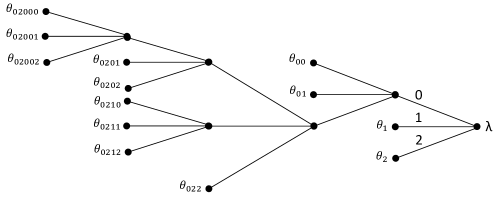
Figure 1: Tree model representation of a 5th order variable-memory chain.

Model prior. Given a maximum depth $D\geq 0$, let $\mathcal{T}(D)$ denote the collection of all proper $m$-ary trees with depth no greater than $D$. In Kontoyiannis et al. (2022), the following prior distribution is introduced on $\mathcal{T}(D)$,

$$\pi(T)=\pi_{D}(T;\beta)=\alpha^{|T|-1}\beta^{|T|-L_{D}(T)}\ ,$$ (2.1)

where $\beta\in(0,1)$ is a hyperparameter, $\alpha$ is given by $\alpha=(1-\beta)^{1/(m-1)}$, $|T|$ is the number of leaves of $T$, and $L_{D}(T)$ is the number of leaves of $T$ at depth $D$.

This prior clearly penalises larger trees by an exponential amount, and larger values of $\beta$ make the penalisation more severe. We adopt the default value $\beta=1-2^{-m+1}$ for $\beta$; see Kontoyiannis et al. (2022) for an extensive discussion of the properties of this prior and the choice of the hyperparameter $\beta$.

Prior on parameters. Given a tree model $T\in\mathcal{T}(D)$, an independent Dirichlet prior with parameters $(1/2,1/2,\ldots,1/2)$ is placed on each $\theta_{s}$, so that:

$$\pi(\theta|T)=\prod_{s\in T}\pi(\theta_{s})=\prod_{s\in T}\text{Dir}(1/2,1/2,\ldots,1/2).\vspace*{-0.1 cm}$$ (2.2)

Let $x=(x_{-D+1},\ldots,x_{0},x_{1},\ldots,x_{n})$ denote a time series with values in $A$. For each $i\leq j$, we write $x_{i}^{j}$ for the segment $(x_{i},x_{i+1},\ldots,x_{j})$, so that $x$ consists of the observations $x_{1}^{n}$ along with an initial context $x_{-D+1}^{0}$ of length $D$.

One of the main observations of Kontoyiannis et al. (2022) is that the prior predictive likelihood, averaged over both models and parameters,

$$P(x)=\sum_{T\in\mathcal{T}(D)}\int_{\theta}P(x|T,\theta)\pi(\theta|T)\pi(T)d\theta,\vspace*{-0.1 cm}$$ (2.3)

can be computed exactly and efficiently by a version of the CTW algorithm (where $P(x|T,\theta)$ denotes the probability of $x$ under model $T$ with parameters $\theta$), which of course facilitates numerous important statistical tasks. For a given time series $x=x_{-D+1}^{n}$, the CTW algorithm uses the estimated probabilities $P_{e,s}$ defined as follows. For any tree model $T\in\mathcal{T}(D)$ and any context $s$ (not necessarily a leaf),

$$P_{e,s}=P_{e}(a_{s})=\frac{\prod_{j=0}^{m-1}[(1/2)(3/2)\cdots(a_{s}(j)-1/2)]}{(m/2)(m/2+1)\cdots(m/2+M_{s}-1)},$$ (2.4)

where the elements of each count vector $a_{s}=(a_{s}(0),a_{s}(1),\ldots,a_{s}(m-1))$ are given by,

$$a_{s}(j)=\mbox{\# times symbol $j\in A$ follows context $s$ in $x_{1}^{n}$},$$ (2.5)

and $M_{s}=a_{s}(0)+a_{s}(1)+\cdots+a_{s}(m-1)$.

CTW: The context tree weighting algorithm.

1. Build the tree $T_{\text{MAX}}$, which is the smallest proper tree that contains all the contexts $x_{i-D+1}^{i},\ i=1,2,\ldots,n$, as leaves. Compute $P_{e,s}$ as given in (2.4) for each node $s$ of $T_{\text{MAX}}$.

2. Starting at the leaves and proceeding recursively towards the root, for each node $s$ of $T_{\text{MAX}}$ compute the weighted probabilities $P_{w,s}$, given by,

   $$P_{w,s}\!=\!\left\{\begin{array}[]{ll}P_{e,s},&\mbox{if $s$ is a leaf,}\\ \beta P_{e,s}+(1-\beta)\prod_{j=0}^{m-1}P_{w,sj},&\mbox{otherwise,}\end{array}\!\!\right.\!\!$$ (2.6)

   where $sj$ is the concatenation of context $s$ and symbol $j$.

As shown in Kontoyiannis et al. (2022), the weighted probability $P_{w,\lambda}$ produced by the CTW algorithm at the root $\lambda$, is indeed exactly equal to the prior predictive likelihood in (2.3). A family of Markov chain Monte Carlo (MCMC) samplers for the posterior $\pi(T|x)$ or $\pi(T,\theta|x)$ were also introduced in Kontoyiannis et al. (2022). However, as will be seen below, the representation of Section 3 leads to a simple i.i.d. MC sampler that typically outperforms these MCMC samplers.

3 Branching process representations

In this section we show that the BCT model prior $\pi(T)=\pi_{D}(T;\beta)$ of (2.1) and the resulting posterior $\pi(T|x)$ both admit natural and easily interpretable representations in terms of simple branching processes. We also discuss how the posterior representation leads to efficient samplers that can be used for model selection and estimation.

3.1 The prior branching process

Given $D\geq 0$ and $\beta\in(0,1)$, let $T=\{\lambda\}$ consist of only the root node $\lambda$ and consider the following procedure:

• If $D=0$, stop.

• If $D>0$, then, with probability $\beta$, mark the root as a leaf and stop, or, with probability $(1-\beta)$, add all $m$ children of $\lambda$ at depth $1$ to $T$. If $D=1$, stop.

• If $D>1$, examine each of the $m$ new nodes, and either mark a node as a leaf with probability $\beta$, or add all $m$ of its children to $T$ with probability $(1-\beta)$, independently from node to node.

• Continue recursively, at each step examining all non-leaf nodes at depths strictly smaller than $D$, until no more eligible nodes remain to be examined.

• Output the resulting tree $T\in\mathcal{T}(D)$.

The above construction is a simple Galton-Watson process (Athreya and Ney, 2004; Harris, 1963) with offspring distribution $(\beta,(1-\beta))$ on $\{0,m\}$, stopped at generation $D$. The following proposition states that the distribution of a tree $T$ generated by this process is exactly the prior $\pi_{D}(T;\beta)$. Note that this also implies that the expression for $\pi_{D}(T;\beta)$ given in (2.1) indeed defines a probability distribution on $\mathcal{T}(D)$, giving an alternative proof of (Kontoyiannis et al., 2022, Lemma 2.1).

Proposition 3.1.

For any $D\geq 0$ and any $\beta\in(0,1)$, the probability that the above branching process produces any particular tree $T\in\mathcal{T}(D)$ is given by $\pi_{D}(T;\beta)$ as in (2.1).

Proof.

When $D=0$, $\mathcal{T}(D)$ consists of a single tree, $T=\{\lambda\}$, which has probability 1 under both $\pi_{D}$ and the branching process construction. Assume $D\geq 1$. Note that every tree $T\in\mathcal{T}(D)$ can be viewed as a collection of a number, $k$, say, of $m$-branches, since every node in $T$ has either zero or $m$ children. The proposition is proven by induction on $k$. The result is trivial for $k=0$, since the only tree with no $m$-branches is $T=\{\lambda\}$ and its probability under both $\pi_{D}$ and the branching process construction is equal to $\beta$.

Suppose the claim of the proposition is true for all trees with $k$ $m$-branches, and let $T^{\prime}\in\mathcal{T}(D)$ consist of $(k+1)$ $m$-branches. Then $T^{\prime}$ can be obtained from some $T\in\mathcal{T}(D)$ that has $k$ $m$-branches, by adding a single $m$-branch to one of its leaves, $s$, say. Two cases are considered.

$(i)$ If $s$ is at depth $D-2$ or smaller, then the probability $\pi_{b}(T^{\prime})$ of $T^{\prime}$ under the branching process construction is,

$$\pi_{b}(T^{\prime})=\frac{\pi_{b}(T)}{\beta}(1-\beta)\beta^{m}=\frac{\pi_{D}(T;\beta)}{\beta}(1-\beta)\beta^{m}=\frac{\alpha^{|T|-1}\beta^{|T|-L_{D}(T)}}{\beta}\alpha^{m-1}\beta^{m},\vspace*{-0.1cm}$$

where the second equality follows from the inductive hypothesis and the third from the definition of $\pi_{D}(T;\beta)$. Therefore, since $|T^{\prime}|=|T|+m-1$ and no leaves are added at depth $D$, so that $L_{D}(T^{\prime})=L_{D}(T)$,

$$\pi_{b}(T^{\prime})=\alpha^{[|T|+m-1]-1}\beta^{|T|+m-1-L_{D}(T)}=\alpha^{|T^{\prime}|-1}\beta^{|T^{\prime}|-L_{D}(T^{\prime})}=\pi_{D}(T^{\prime};\beta),$$

as required.

$(ii)$ If $s$ is at depth $D-1$, we similarly find that,

$$\pi_{b}(T^{\prime})=\frac{\pi_{b}(T)}{\beta}(1-\beta)=\frac{\pi_{D}(T;\beta)}{\beta}(1-\beta)=\frac{\alpha^{|T|-1}\beta^{|T|-L_{D}(T)}}{\beta}\alpha^{m-1},\vspace*{-0.1 cm}$$

and since $|T^{\prime}|=|T|+m-1$, but now, $L_{D}(T^{\prime})=L_{D}(T)+m$,

$$\pi_{b}(T^{\prime})=\alpha^{[|T|+m-1]-1}\beta^{[|T|+m-1]-[L_{D}(T)+m]}=\alpha^{|T^{\prime}|-1}\beta^{|T^{\prime}|-L_{D}(T^{\prime})}=\pi_{D}(T^{\prime};\beta),$$

completing the proof.     $\Box$

Apart from being aesthetically appealing, this representation also offers a simple and practical way of sampling from $\pi_{D}(T;\beta)$. Moreover, using well-known properties of the Galton-Watson process we can perform some direct computations that offer better insight into the nature and specific properties of the BCT prior.

Interpretation and choice of $\beta$. The branching process description of $\pi_{D}(T,\beta)$ further clarifies the role of the hyperparameter $\beta$: It is exactly the probability that, when a node is added to the tree $T$, it is marked as a leaf and its children are not included in $T$.

In terms of choosing the value of the hyperparameter $\beta$ appropriately, recall that, for a Galton-Watson process, the expected number of children of each node, in this case $\rho=m(1-\beta)$, governs the probability of extinction $P_{e}$: If $\rho\leq 1$ we have $P_{e}=1$, whereas if $\rho>1$, $P_{e}$ is strictly less than one. Therefore, in the binary case $m=2$, the original choice $\beta=1/2$ used in the CTW algorithm gives an expected number of children equal to the critical value $\rho=1$. This suggests that a reasonable choice for general alphabets could be $\beta=1-1/m$, which keeps $\rho=1$, so that the resulting prior would have similar qualitative characteristics with the well-studied binary case. This is also in line with the observation of Kontoyiannis et al. (2022) that $\beta$ should decrease with $m$.

Now suppose $T$ is a random model generated by the prior and let $L_{d}(T)$ denote the number of nodes at depth $d=0,1,\ldots,D$. Then, standard Galton-Watson theory (Athreya and Ney, 2004; Harris, 1963) provides the useful expressions,

$$\mathbb{E}\left[L_{d}(T)\right]=\rho^{d},\quad\quad\quad\text{Var}\left[L_{d}(T)\right]=\left\{\begin{array}[]{ll}\sigma^{2}d,&\mbox{if $\rho=1$,}\\ \sigma^{2}\rho^{d-1}\frac{1-\rho^{d}}{1-\rho},&\mbox{if $\rho\neq 1$},\end{array}\!\!\right.\vspace*{-0.15 cm}$$

where $\sigma^{2}=m^{2}\beta(1-\beta)$.

3.2 The posterior branching process

Given a time series $x=x_{-D+1}^{n}$, a maximum depth $D$, and $\beta\in(0,1)$, for any context $s$ with length strictly smaller than $D$ we define the branching probabilities $P_{b,s}$ as,

$$P_{b,s}:=\frac{\beta P_{e,s}}{P_{w,s}},\vspace*{-0.1 cm}$$ (3.1)

where the estimated and weighted probabilities, $P_{e,s}$ and $P_{w,s}$, are defined in (2.4)-(2.6), and with the convention that $P_{b,s}=\beta$ for all contexts $s$ that do not appear in $x$. Starting with $T=\{\lambda\}$, the following construction produces a sample model $T\in{\mathcal{T}}(D)$ from the model posterior $\pi(T|x)$:

• If $D=0$, stop.

• If $D>0$, then, with probability $P_{b,\lambda}$, mark the root as a leaf and stop, or, with probability $(1-P_{b,\lambda})$, add all $m$ children of $\lambda$ at depth $1$ to $T$. If $D=1$, stop.

• If $D>1$, examine each of the $m$ new nodes and either mark a node $s$ as a leaf with probability $P_{b,s}$, or add all $m$ of its children to $T$ with probability $(1-P_{b,s})$, independently from node to node.

• Continue recursively, at each step examining all non-leaf nodes at depths strictly smaller than $D$, until no more eligible nodes remain.

• Output the resulting tree $T\in\mathcal{T}(D)$.

Proposition 3.2.

For any $D\geq 0$ and any $\beta\in(0,1)$, the probability that the above branching process produces any particular tree $T\in\mathcal{T}(D)$ is given by $\pi(T|x)$.

The proof, which follows along the same lines as that of Proposition 3.1, is given in Section A of the supplementary material. It is perhaps somewhat remarkable that the posterior $\pi(T|x)$ on the vast model space $\mathcal{T}(D)$ admits such a simple description. Indeed, the posterior branching process is of exactly the same form as that of the prior, which can then naturally be viewed as a conjugate prior on $\mathcal{T}(D)$.

Model posterior probabilities. Proposition 3.2 allows us to write an exact expression for the posterior of any model $T\in\mathcal{T}(D)$ in terms of the branching probabilities $P_{b,s}$,

$$\pi(T|x)=\prod_{s\in T_{o}}\left(1-P_{b,s}\right)\prod_{s\in T}P_{b,s},\vspace*{-0.1 cm}$$ (3.2)

where $T_{o}$ denotes the set of all internal nodes of $T$, and with the convention that $P_{b,s}=1$ for all leaves of $T$ at depth $d=D$. This expression will be the starting point in the proofs of the asymptotic results of Section 4 for $\pi(T|x)$.

In terms of inference, the main utility of Proposition 3.2 is that it offers a practical way of obtaining exact i.i.d. samples directly from the model posterior, as described in the next section.

3.3 Sampling from the posterior

The branching process representation of $\pi(T|x)$ readily leads to a simple way for obtaining i.i.d. samples $\{T^{(i)}\}$ from the posterior on model space. And since the full conditional density of the parameters $\pi(\theta|T,x)$ is explicitly identified by Kontoyiannis et al. (2022) as a product of Dirichlet densities,

$$\pi(\theta|T,x)=\prod_{s\in T}\text{Dir}\left(1/2+a_{s}(0),1/2+a_{s}(1),\ldots,1/2+a_{s}(m-1)\right),$$ (3.3)

for each $T^{(i)}$ we can draw a conditionally independent sample $\theta^{(i)}\sim\pi(\theta|T^{(i)},x)$, producing a sequence of exact i.i.d. samples $\{(T^{(i)},\theta^{(i)})\}$ from the joint posterior $\pi(T,\theta|x)$.

This facilitates numerous applications. For example, effective parameter estimation can be performed by simply keeping the samples $\{\theta^{(i)}\}$, which come from the marginal posterior distribution $\pi(\theta|x)$. Similarly, Markov order estimation can be performed by collecting the sequence of maximum depths of the models $\{T^{(i)}\}$. And in model selection tasks, the model posterior can be extensively explored, offering better insight and deeper understanding of the underlying structure and dependencies present in the data.

Although a family of MCMC samplers was introduced and successfully used for the same tasks in Kontoyiannis et al. (2022), MCMC sampling has well-known limitations and drawbacks, including potentially slow mixing, high correlation between samples, and the need for convergence diagnostics (Gelman and Rubin, 1992; Cowles and Carlin, 1996; Robert and Casella, 2004). Partly for these reasons, being able to obtain i.i.d. samples from the posterior is generally much more desirable, as illustrated in Section 5.1.

Estimation of general functionals. Consider the general Bayesian estimation problem, where the goal is to estimate an arbitrary functional $F=F(T,\theta)$ of the underlying variable-memory chain, based on data $x$. Using the above sampler, the entire posterior distribution of the statistic $F$ can be explored, by considering the i.i.d. samples $F^{(i)}=F(T^{(i)},\theta^{(i)})$, distributed according to the desired posterior $\pi(F|x)$.

In connection with classical estimation techniques, and in order to evaluate estimation performance more easily in practice, several reasonable point estimates can also be obtained. The most common choices are the empirical average approximation to the posterior mean,

$$\widehat{F}_{\text{MC}}=\frac{1}{N}\sum_{i=1}^{N}F^{(i)}=\frac{1}{N}\sum_{i=1}^{N}F(T^{(i)},\theta^{(i)}),$$ (3.4)

or the posterior mode, i.e., the maximum a posteriori probability (MAP) estimate, $\widehat{F}_{\text{MAP}}$. In cases where the conditional mean $\bar{F}(T)={E}\big{(}F(T,\theta)|x,T\big{)}$ can be computed for any model $T$ (as e.g. in the case of parameter estimation), a lower-variance Rao-Blackwellised estimate (Blackwell, 1947; Gelfand and Smith, 1990) for the posterior mean can also be obtained as,

$$\widehat{F}_{\text{RB}}=\frac{1}{N}\sum_{i=1}^{N}\bar{F}(T^{(i)}).$$

Importantly, as this posterior sampler provides access to the entire posterior distribution $\pi(F|x)$ of the statistic of interest $F$, standard Bayesian methodology can be applied to quantify the resulting uncertainty of any estimator $\hat{F}$, for example by obtaining credible intervals in terms of the posterior $\pi(F|x)$.

An interesting special case of particular importance in practice is the estimation of the entropy rate $H$ of the underlying process, $F(T,\theta)=H(T,\theta)$. The performance of all methods discussed above, with emphasis on the estimation of the entropy rate, is illustrated through simulated experiments and real-world applications in Section 5.2.

4 Theoretical results

Using the branching process representation of Proposition 3.2, we show how to derive precise results on the asymptotic behaviour of the BCT posterior $\pi(T|x)$ on model space, and provide an explicit, useful expression for the posterior predictive distribution.

Let $\{X_{n}\}$ be a variable-memory chain with model $T\in\mathcal{T}(D)$. The specific model $T$ that describes the chain is typically not unique, for the same reason, e.g., that every i.i.d. process can also trivially be described as a first-order Markov chain: Adding $m$ children to any leaf of $T$ which is not at maximal depth, and giving each of them the same parameters as their parent, leaves the distribution of the chain unchanged.

The natural main goal in model selection is to identify the “minimal” model, i.e., the smallest model that can fully describe the distribution of the chain. A model $T\in\mathcal{T}(D)$ is called minimal if every $m$-tuple of leaves $\{sj\;;\;j=0,1,\ldots,m-1\}$ in $T$ contains at least two with non-identical parameters, i.e., there are $j\neq j^{\prime}$ such that $\theta_{sj}\neq\theta_{sj^{\prime}}$. It is easy to see that every $D$th order Markov chain $\{X_{n}\}$ has a unique minimal model $T^{*}\in\mathcal{T}(D)$.

A variable-memory chain $\{X_{n}\}$ with model $T\in\mathcal{T}(D)$ and with associated parameters $\theta=\{\theta_{s};s\in T\}$ is ergodic, if the corresponding first-order chain $\{Z_{n}:=X_{n-D+1}^{n};n\geq 1\}$ taking values in $A^{D}$ is irreducible and aperiodic. In order to avoid uninteresting technicalities, in most of our results we will assume that the data are generated by a positive-ergodic chain $\{X_{n}\}$, namely that all its parameters $\theta_{s}(j)$ are nonzero, so that its unique stationary distribution $\pi$ gives strictly positive probability to all finite contexts $s$.

4.1 Posterior consistency and concentration

Our first theorem is a strong consistency result, which states that, if the data $x=x_{-D+1}^{n}$ are generated by an ergodic chain with minimal model $T^{*}\in\mathcal{T}(D)$, then the model posterior asymptotically almost surely (a.s.) concentrates on $T^{*}$. Theorem 4.1 both strengthens and generalises a weaker result on the asymptotic behaviour of the MAP model established in (Willems et al., 1993, Theorem 8).

Theorem 4.1.

Let $X_{-D+1}^{n}=(X_{-D+1},\ldots,X_{0},X_{1},\ldots,X_{n})$ be a time series generated by a positive-ergodic, variable-memory chain $\{X_{n}\}$ with minimal model $T^{*}\in\mathcal{T}(D)$. For any value of the prior hyperparameter $\beta\in(0,1)$, the posterior distribution over models concentrates on $T^{*}$, i.e.,

$$\pi(T^{*}|X_{-D+1}^{n})\to 1,\quad\text{a.s., as }n\to\infty.$$

Proof.

Recalling the posterior representation in (3.2), it suffices to show that, as $n\to\infty$, $P_{b,s}\to 0$ a.s. for all internal nodes of $T^{*}$, and $P_{b,s}\to 1$ a.s. for all leaves of $T^{*}$. These two claims are established in Lemmas 4.2 and 4.3 below.     $\Box$

We first recall the following simple bounds on the estimated probabilities $P_{e,s}$; see Krichevsky and Trofimov (1981); Xie and Barron (2000) and (Catoni, 2004, Ch. 1).

Lemma 4.1.

For every node $s$ with count vector $a_{s}=(a_{s}(0),a_{s}(1),\ldots,a_{s}(m-1))$ and $M_{s}=a_{s}(0)+\cdots+a_{s}(m-1)$, the estimated probabilities $P_{e,s}$ of (2.4) satisfy:

$$\log P_{e,s}\geq \sum_{j=0}^{m-1}a_{s}(j)\log\frac{a_{s}(j)}{M_{s}}-\frac{m-1}{2}\log M_{s}-\log m;$$ (4.1)

$$\log P_{e,s}\leq \sum_{j=0}^{m-1}a_{s}(j)\log\frac{a_{s}(j)}{M_{s}}-\frac{m-1}{2}\log\frac{M_{s}}{2\pi}-\log\frac{\pi^{m/2}}{\Gamma(m/2)}.$$ (4.2)

[Throughout the paper, $\log\equiv\log_{e}$ denotes the natural logarithm.] Lemma 4.2 is a generalisation of (Jiao et al., 2013, Lemma 12).

Lemma 4.2.

Under the assumptions of Theorem 4.1, for every internal node $s$ of $T^{*}$, the branching probability $P_{b,s}\to 0$, a.s., as $n\to\infty$.

Proof.

As the complete proof is quite involved, only the main and more interesting part of the argument is given here, with the remaining details given in Section B.1 of the supplementary material. We begin by observing that,

$$P_{b,s}=\frac{\beta P_{e,s}}{P_{w,s}}=\frac{\beta P_{e,s}}{\beta P_{e,s}+(1-\beta)\prod_{j}P_{w,sj}} =\frac{1}{1+{(1-\beta)}/{\beta}\ {\prod_{j}P_{w,sj}}/{P_{e,s}}}$$ (4.3)

$$\leq\frac{1}{1+c_{0}\ {\prod_{j}P_{e,sj}}/{P_{e,s}}},$$ (4.4)

for some constant $c_{0}$, where in the last step we used that either $P_{w,sj}\geq\beta P_{e,sj}$ or $P_{w,sj}=P_{e,sj}$. Therefore, it suffices to show that $P_{e,s}\big{/}\prod_{j}P_{e,sj}\to 0$, a.s., as $n\to\infty$.

Let $s$ be a fixed finite context, and let $X$ and $J$ denote the random variables corresponding to the symbols that follow and precede $s$, respectively, under the stationary distribution of $\{X_{n}\}$. Using Lemma 4.1 and the ergodic theorem for Markov chains, it is shown in Section B.1 of the supplementary material that,

$$\log P_{e,s}-\sum_{j}\log P_{e,sj}=-nI(X;J|s)\pi(s)+o(n),\quad\text{a.s.},$$ (4.5)

where $I(X;J|s)$ is the conditional mutual information between $X$ and $J$ given $s$ (Cover and Thomas, 2012, Ch. 2). This mutual information is always nonnegative, and it is zero if and only if $X$ and $J$ are conditionally independent given $s$.

For any internal node $s$ that is a parent of leaves of $T^{*}$, the minimality of $T^{*}$ implies that $X$ and $J$ are not conditionally independent given $s$, as there exist $j\neq j^{\prime}$ such that $\theta_{sj}\neq\theta_{sj^{\prime}}$, so that $\theta_{sj}$ depends on $j$. Therefore, $I(X;J|s)>0$ and $\pi(s)>0$ by assumption, so (4.5) implies that $\log P_{e,s}-\sum_{j}\log P_{e,sj}\to-\infty$, a.s., as required.

For the general case of internal nodes that may not be parents of leaves, a simple iterative argument is given in Section B.1 of supplementary material establishing the same result in that case as well, and completing the proof of the lemma.     $\Box$

Lemma 4.3.

Under the assumptions of Theorem 4.1, for every leaf $s$ of $T^{*}$, the branching probability $P_{b,s}\to 1$, a.s., as $n\to\infty$.

Proof.

As with the previous lemma, we only give an outline of the main interesting steps in the proof here; complete details are provided in Section B.2 of the supplementary material.

By definition, for any leaf $s$ of $T^{*}$ (and also for any ‘external’ node $s$, that is, any context $s$ not in $T^{*}$), we have $I(X;J|s)=0$ because of conditional independence. Therefore, we need to consider the higher-order terms in the asymptotic expansion of (4.5). Using Lemma 4.1, the ergodic theorem, and the law of the iterated logarithm (LIL) for Markov chains, it is shown in Section B.2 of the supplementary material that here,

$$\sum_{j}\log P_{e,sj}-\log P_{e,s}\leq-\frac{(m-1)^{2}}{2}\log n+O(\log\log n),\quad\text{a.s.}$$ (4.6)

This implies that $\sum_{j}\log P_{e,sj}-\log P_{e,s}\to-\infty$, so that $\prod_{j}P_{e,sj}/{P_{e,s}}\to 0$, a.s.

The last step of the proof, namely that for any leaf $s$ of $T^{*}$, $\prod_{j}P_{e,sj}/{P_{e,s}}\to 0$ also implies that $\prod_{j}P_{w,sj}/{P_{e,s}}\to 0$, a.s., so that, by (4.3), $P_{b,s}\to 1$, a.s., is given in Section B.2 of the supplementary material.     $\Box$

Our next result is a refinement of Theorem 4.1, which characterises the rate at which the posterior probability of $T^{*}$ converges to 1.

Theorem 4.2.

Let $X_{-D+1}^{n}$ be a time series generated by a positive-ergodic variable-memory chain $\{X_{n}\}$ with minimal model $T^{*}\in\mathcal{T}(D)$. For any value of the prior hyperparameter $\beta\in(0,1)$ and any $\epsilon>0$, we have, as $n\to\infty$:

$$\pi(T^{*}|X_{-D+1}^{n})=1-O\left(n^{-\frac{(m-1)^{2}}{2}+\epsilon}\right),\quad\text{a.s.}$$

The proof of Theorem 4.2 is given in Section B.3 of the supplementary material. In fact, as discussed at the end of Section B.3, the proof also reveals that a stronger statement can be made about the rate in the case of full $D$th order Markov chains:

Corollary 4.1.

If $\{X_{n}\}$ is a genuinely $D$th order chain in that its minimal model $T^{*}$ is the complete tree of depth $D$, then its posterior probability $\pi(T^{*}|X_{-D+1}^{n})$ almost surely converges to 1 at an exponential rate.

4.2 Out-of-class modelling

In this section we consider the behaviour of the posterior distribution $\pi(T|x)$ on models $T\in{\mathcal{T}}(D)$ when the time series $x$ is not generated by a chain from the model class ${\mathcal{T}}(D)$, but from a general stationary and ergodic process $\{X_{n}\}$ with possibly infinite memory. We first give an explicit description of the “limiting” model $T_{\infty}\in{\mathcal{T}}(D)$ on which the posterior $\pi(T|x)$ concentrates when the observations are generated by a general process outside ${\mathcal{T}}(D)$, and then we give conditions under which $T_{\infty}$ is structurally “as close as possible” to the true underlying model.

Description of $T_{\infty}$. Recall that, for any context $s$, we write $X$ and $J$ for the random variables corresponding to the symbols that follow and precede $s$, respectively. The limiting tree $T_{\infty}\in{\mathcal{T}}(D)$ corresponding to a general stationary process $\{X_{n}\}$ with values in $A$ can be constructed via the following procedure:

• Take $T_{\infty}$ to be the empty tree.

• Starting with the nodes at depth $d=D-1$, for each such $s$, if $I(X;J|s)>0$, then add $s$ to $T_{\infty}$ along with all its children and all its ancestors; that is, add the complete path from the root $\lambda$ to the children of $s$.

• After all nodes $s$ at depth $d=D-1$ have been examined, examine all possible nodes $s$ at depth $d=D-2$ that are not already included in $T_{\infty}$, and repeat the same process.

• Continue recursively towards the root, until all nodes at all depths $0\leq d\leq D-1$ have been examined.

• For any node already in $T_{\infty}$ at depth $d\leq D-1$, such that only some but not all $m$ of its children are included in $T_{\infty}$, add the missing children to $T_{\infty}$ so that it becomes proper.

• Output $T_{\infty}$.

In order to state our results we need to impose two additional conditions on the underlying data-generating process. Suppose $\{X_{n}\}$ is stationary. Without loss of generality (by Kolmogorov’s extension theorem) we may consider the two-sided version of the process, $\{X_{n}\;;\;n\in{\mathbb{Z}}\}$. Its $\alpha$-mixing coefficients (Ibragimov, 1962; Philipp and Stout, 1975) are defined as,

$$\alpha_{n}=\sup_{A\in\mathcal{A},\;B\in\mathcal{B}}|\mathbb{P}(A\cap B)-\mathbb{P}(A)\mathbb{P}(B)|,$$ (4.7)

where $\mathcal{A}$ and $\mathcal{B}$ denote the $\sigma$-algebras, $\sigma(\ldots,X_{-1},X_{0})$ and $\sigma(X_{n},X_{n+1},\ldots)$, respectively. We will need a mixing condition and a positivity condition for our results:

$$\sum_{n=1}^{\infty}\alpha_{n}^{\delta/(2+\delta)}<\infty\;\mbox{for some}\;\delta>0,\quad\mbox{and}\quad{\mathbb{P}}(X_{0}^{D}=x_{0}^{D})>0\;\mbox{for all}\;x_{0}^{D}\in A^{D+1}.$$ (4.8)

Theorem 4.3.

Let $X_{-D+1}^{n}$ be a time series generated by a stationary ergodic process $\{X_{n}\}$ satisfying the assumptions (4.8), and let $T_{\infty}\in{\mathcal{T}}(D)$ be given by the above construction. Then, for any value of the prior hyperparameter $\beta\in(0,1)$ we have:

$$\pi(T_{\infty}|X_{-D+1}^{n})\to 1,\quad\text{a.s., as }n\to\infty.$$

The proof of Theorem 4.3 follows along exactly the same lines as the earlier proof of Theorem 4.1. Instead of the ergodic theorem for Markov chains (Chung, 1967, p. 92) we now use Birkhoff’s ergodic theorem (Breiman, 1992, Ch. 6), and instead of the LIL for Markov chains we apply the general LIL for functions of blocks of an ergodic process, which follows, as usual, from the almost-sure invariance principle (Philipp and Stout, 1975; Rio, 1995; Zhao and Woodroofe, 2008). The mixing condition in (4.8) was chosen as one of the simplest ones that guarantee this general version of the LIL.

Regarding the overall structure of the proof, all the earlier asymptotic expansions of the branching probabilities still remain valid, including (4.5) and (4.6). The only possible difference might be at the boundary conditions that are required as a starting point for the iterative argument in the proof of Lemma 4.2, since the actual “leaves” of the true underlying model of $\{X_{n}\}$ are not necessarily at depth $d\leq D$ here. But, as before, all branching probabilities $P_{b,s}$ tend either to 0 or to 1, depending on whether the mutual information condition that appears in the description of $T_{\infty}$ holds or not. Specifically, starting from nodes $s$ at depth $d=D-1$, if $I(X;J|s)=0$ then we are in the same situation as in Lemma 4.3, so that $P_{b,s}\to 1$, and all children of $s$ are pruned. On the other hand, if $I(X;J|s)>0,$ then $P_{b,s}\to 0$, and by the same iterative argument, $P_{b,u}\to 0$ for all ancestors $u$ of node $s$ as well.

Analogous comments apply to the proof of Theorem 4.4, which is again a refinement characterising the rate at which the posterior probability of $T_{\infty}$ converges to 1.

Theorem 4.4.

Let $X_{-D+1}^{n}$ be a time series generated by a stationary ergodic process $\{X_{n}\}$ satisfying the assumptions (4.8), and let $T_{\infty}$ be its limiting model in ${\mathcal{T}}(D)$. Then, for any $\beta\in(0,1)$ and any $\epsilon>0$, as $n\to\infty$ we have:

$$\pi(T_{\infty}|X_{-D+1}^{n})=1-O\left(n^{-\frac{(m-1)^{2}}{2}+\epsilon}\right),\quad\mbox{a.s.}$$

In general, it is natural to expect that $T_{\infty}$ should be “as close as possible” in some sense to the true underlying model $T^{*}$, and this is indeed what is most often observed in applications: $T_{\infty}$ being the same as $T^{*}$ truncated to depth $D$.

But this is not always the case. For example, recall the 3rd order chain $\{X_{n}\}$ considered in Example 5.2 of Kontoyiannis et al. (2022), also described as having a “bimodal posterior” in Section 5.2. There, $T^{*}$ is the complete $m$-ary tree of depth 3 (with $m=6$), but $X_{n}$ depends on $(X_{n-1},X_{n-2},X_{n-3})$ only via $X_{n-3}$. For that reason, the limiting model $T_{\infty}$ in ${\cal T}(D)$ with $D=1$ or $D=2$ is not $T^{*}$ truncated at depth $D$, but rather the empty tree $\{\lambda\}$ consisting of only the root node $\lambda$.

Fortunately, we can read a simple necessary and sufficient condition for the “expected” behaviour to occur from the definition of $T_{\infty}$ itself. Let $\{X_{n}\}$ be a stationary and ergodic process on the finite alphabet $A$. From the description of Csiszár and Talata (2006), it is easy to see that there is a unique minimal context tree model $T^{*}$ for $\{X_{n}\}$ of possibly infinite depth. Let $T^{*}_{|D}$ be $T^{*}$ truncated at depth $D$, and write $N_{D-1}(T^{*})$ for the set of all internal nodes of $T^{*}$ at depth $d=D-1$ whose children exist in $T^{*}$ (at depth $D$) but are not leaves of $T^{*}$.

Corollary 4.2.

The limiting model $T_{\infty}=T^{*}_{|D}$ if and only if $I(X;J|s)>0$ for all the nodes $s\in N_{D-1}(T^{*})$.

Proof.

The result follows directly from the definition of $T_{\infty}$ combined with the observation that the condition $I(X;J|s)>0$ is already satisfied for all nodes $s$ of $T^{*}$ at depth $d=D-1$ whose children are leaves of $T^{*}$.     $\Box$

4.3 The posterior predictive distribution

The branching process representation of the posterior can also be used to facilitate practically useful computations. In Proposition 4.1, an exact expression is given for the posterior predictive distribution $P\left(x_{n+1}|x_{-D+1}^{n}\right)$ in terms of the branching probabilities $P_{b,s}$.

Proposition 4.1.

The posterior predictive distribution is given by,

$$P\left(x_{n+1}|x_{-D+1}^{n}\right)=\sum_{i=0}^{D}\left(\frac{a_{s^{(i)}}\left(x_{n+1}\right)+1/2}{M_{s^{(i)}}+m/2}\right)\gamma_{i},$$ (4.9)

where, for $0\leq i\leq D$, the string $s^{(i)}$ is the context of length $i$ preceding $x_{n+1}$, and $\gamma_{i}$ is the posterior probability that node $s^{(i)}$ is a leaf, given by,

$$\gamma_{i}\!=\!\left\{\begin{array}[]{ll}P_{b,\lambda},&i=0,\\ \prod_{k=0}^{i-1}\left(1-P_{b,s^{(k)}}\right)P_{b,s^{(i)}},&1\leq i\leq D-1,\\ \prod_{k=0}^{D-1}\left(1-P_{b,s^{(k)}}\right),&i=D.\end{array}\!\!\right.\!\!$$ (4.10)

Proof.

Writing $x=x_{-D+1}^{n}$, the posterior predictive distribution can be expressed as,

$$P\left(x_{n+1}|x\right)=\sum_{T\in\mathcal{T}(D)}P\left(x_{n+1}|T,x\right)\pi(T|x).$$ (4.11)

For any tree ${T\in\mathcal{T}(D)}$, exactly one of the contexts $s^{(i)}$, $0\leq i\leq D$, is a leaf of the tree. For every $0\leq i\leq D$, define the subset $\mathcal{T}_{i}(D)\subset\mathcal{T}(D)$ to be the collection of trees $T\in\mathcal{T}(D)$ such that the context of $x_{n+1}$ that is a leaf of $T$ is $s^{(i)}$; these $\mathcal{T}_{i}(D)$ are disjoint and their union is $\mathcal{T}(D)$.

The key observation here is that $P(x_{n+1}|T,x)$ is the same for all trees $T\in\mathcal{T}_{i}(D)$, since,

$$P(x_{n+1}|T,x)= \int_{\theta}P(x_{n+1}|T,\theta,x)\pi(\theta|T,x)\ d\theta$$

$$= \int_{\theta_{s^{(i)}}}P(x_{n+1}|T,\theta_{s^{(i)}},x)\pi(\theta_{s^{(i)}}|T,x)\ d\theta_{s^{(i)}}$$

$$= \int_{\theta_{s^{(i)}}}\theta_{s^{(i)}}\left(x_{n+1}\right)\pi(\theta_{s^{(i)}}|T,x)\ d\theta_{s^{(i)}}=\frac{a_{s^{(i)}}\left(x_{n+1}\right)+1/2}{M_{s^{(i)}}+m/2},$$ (4.12)

where we used the full conditional density of the parameters in (3.3). So, from (4.11),

$$P\left(x_{n+1}|x\right)=\sum_{i=0}^{D}\sum_{T\in\mathcal{T}_{i}(D)}P\left(x_{n+1}|T,x\right)\pi(T|x)=\sum_{i=0}^{D}\frac{a_{s^{(i)}}\left(x_{n+1}\right)+1/2}{M_{s^{(i)}}+m/2}\sum_{T\in\mathcal{T}_{i}(D)}\pi(T|x),$$

which completes the proof upon noticing that the last sum $\sum_{T\in\mathcal{T}_{i}(D)}\pi(T|x)$ is exactly the posterior probability that node $s^{(i)}$ is a leaf, namely, $\gamma_{i}$ as in (4.10).     $\Box$

5 Experimental results

Being able to obtain exact i.i.d. samples from the posterior is generally more desirable and typically leads to more efficient estimation than using approximate MCMC samples. In Section 5.1 we offer empirical evidence justifying this statement in the present setting through a simple simulation example. Then in Section 5.2 we present the results of a careful empirical study of the natural entropy estimator induced by the BCT framework, compared against a number of the most common alternative estimators, on three simulated and three real-world data sets.

5.1 Comparison with MCMC

Consider $n=1000$ observations generated from a 5th order, ternary chain, with model given by the context tree of Figure 1 in Section 2 (the values of the parameters $\theta=\{\theta_{s};s\in T\}$ are given in Section C of the supplementary material). A simple and effective convergence diagnostic here (which can also be viewed as an example of an estimation problem) is the examination of the frequency with which the MAP model, $T_{1}^{*}$, appears in the i.i.d. or the MCMC sample trajectory. The model $T_{1}^{*}$ can be identified by the BCT algorithm and its posterior probability $\pi(T_{1}^{*}|x)$ can be computed, as in (Kontoyiannis et al., 2022).

Figure 2: Frequency of $T_{1}^{*}$. Blue: MCMC estimates. Red: i.i.d. estimates. In each case, the five graphs correspond to five independent repetitions of the experiment with $N=1000$ simulated samples. The horizontal line is the limiting frequency, $\pi(T_{1}^{*}|x)$.

As shown in Figure 2, the estimates based on the random-walk MCMC sampler of Kontoyiannis et al. (2022) and on the i.i.d. sampler of Section 3.3 both appear to converge quite quickly, with the corresponding MCMC estimates converging significantly more slowly. In 50 independent repetitions of the same experiment (with $N=1000$ simulated samples in each run), the estimated variance of the MCMC estimates (0.0084) was found to be larger than that for the i.i.d. estimates ($1.4\times 10^{-4}$), by a factor of around 60.

Figure 3 shows the trace plots (Roy, 2020) obtained from $N=10000$ simulated samples from the MCMC and i.i.d. samplers, which can be used to monitor the log-posterior in each case. It is immediately evident that the i.i.d. sampler is more efficient in exploring the effective support of the posterior.

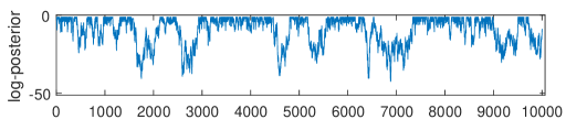
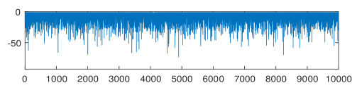
Figure 3: Trace plots showing the log-posterior, $\log\pi(T^{(i)}|x)$, at each iteration. Top: MCMC samples. Bottom: i.i.d. samples.

As expected, the i.i.d. sampler has superior performance compared to the MCMC sampler, both in terms of estimation and in terms of mixing. Also, although the two types of samplers have comparable complexity in terms of computation time and memory requirements, the structure of the i.i.d. sampler is much simpler, giving a much easier implementation. In view of these observations, in the following section we only employ the i.i.d. sampler for the purposes of entropy estimation.

5.2 Entropy estimation

Estimating the entropy rate from empirical data – in this case, a discrete time series – is an important and timely problem that has received a lot of attention in the recent literature, in connection with questions in many areas including neuroscience (Timme and Lapish, 2018), natural language modelling (Willems et al., 2016), animal communication (Kershenbaum, 2014), and cryptography (Simion, 2020), among others; see, e.g., the recent literature reviews by Verdú (2019) and Feutrill and Roughan (2021). The well-known difficulties of entropy estimation stemming from the nonlinear nature of the entropy rate functional and its dependence on the entire process distribution are discussed in the references listed above.

For a general process $\{X_{n}\}$ on a finite alphabet, the entropy rate $\bar{H}$ is defined as the limit $\bar{H}=\lim_{n\to\infty}(1/n)H(X_{1}^{n})$, whenever the limit exists, where $H(X_{1}^{n})$ denotes the usual Shannon entropy (in nats rather than bits, as we take logarithms to the base $e$) of the discrete random vector $X_{1}^{n}$. For an ergodic, first-order Markov chain $\{X_{n}\}$, $\bar{H}$ can be expressed as,

$$\bar{H}=-\sum_{i,j\in S}\pi(i)P_{ij}\log P_{ij},$$ (5.1)

where $S$ is the state space of $\{X_{n}\}$, and $(P_{ij})$ and $(\pi(i))$ denote its transition matrix and its stationary distribution, respectively.

An analogous formula can be written for the entropy rate of any ergodic variable-memory chain with model $T\in{\mathcal{T}}(D)$, by viewing it as a full $D$th order chain and considering blocks of length $(D+1)$, as usual; cf. Cover and Thomas (2012). This means that $\bar{H}$ can be expressed as an explicit function $\bar{H}=H(T,\theta)$ of the model and parameters.

Therefore, given a time series $x$, using the MC sampler of Section 3.3 to produce i.i.d. samples $(T^{(i)},\theta^{(i)})$ from $\pi(T,\theta|x)$, we can obtain i.i.d. samples $H^{(i)}=H(T^{(i)},\theta^{(i)})$ from the posterior $\pi(\bar{H}|x)$ of the entropy rate. The calculation of each $H^{(i)}=H(T^{(i)},\theta^{(i)})$ is straightforward and only requires the computation of the stationary distribution $\pi$ of the induced first-order chain that corresponds to taking blocks of size [depth$(T^{(i)})+1$]. The only potential difficulty is if either the depth of $T^{(i)}$ or the alphabet size $m$ are so large that the computation of $\pi$ becomes computationally expensive. In such cases, $H^{(i)}$ can be computed approximately by including an additional Monte Carlo step: Generate a sufficiently long random sample $Y_{-D+1}^{M}$ from the chain $(T^{(i)},\theta^{(i)})$, and calculate:

$$H^{(i)}\approx-\frac{1}{M}\log P(Y_{1}^{M}|Y_{-D+1}^{0},T^{(i)},\theta^{(i)}).$$ (5.2)

The ergodic theorem and the central limit theorem for Markov chains (Chung, 1967; Meyn and Tweedie, 2012) then guarantee the accuracy of (5.2).

In the remainder of this section, the BCT estimator (with maximum model depth $D=10$) is compared with the state-of-the-art approaches, as identified by Gao et al. (2008) and Verdú (2019) and summarised below. The BCT estimator is found to generally give the most reliable estimates on a variety of different types of simulated and real-world data. Moreover, compared to most existing approaches that give simple point estimates (sometimes accompanied by confidence intervals), the BCT estimator has the additional advantage that it provides the entire posterior distribution $\pi(\bar{H}|x)$.

Plug-in estimator. Motivated by the definition of the entropy rate, the simplest and one of the most commonly used estimators of the entropy rate is the per-sample entropy of the empirical distribution of $k$-blocks. Letting $\widehat{p}_{k}(y_{1}^{k})$, $y_{1}^{k}\in A^{k}$, denote the empirical distribution of $k$-blocks induced by the data on $A^{k}$, the plug-in or maximum-likelihood estimator is simply, $\widehat{H}_{k}=(1/k)H(\widehat{p}_{k})$. The main advantage of this estimator is its simplicity. Well-known drawbacks include its high variance due to undersampling, and the difficulty in choosing appropriate block-lengths $k$ effectively.

Lempel-Ziv estimator. Among the numerous match-length-based entropy estimators that have been derived from the Lempel-Ziv family of data compression algorithms, we consider the increasing-window estimator of Gao et al. (2008), identified there as the most effective one. For every position $i$ in the observed data, let $\ell_{i}$ denote the length of the longest segment $x_{i}^{i+\ell_{i}-1}$ starting at $i$ which also appears somewhere in the window $x_{0}^{i-1}$ preceding $i$. Writing $L_{i}=1+\ell_{i}$ for each $i$, the relevant estimator is,

$$\widehat{H}_{\text{LZ}}=\frac{1}{n}\sum_{i=2}^{n}\frac{\log i}{L_{i}}.\vspace*{-0.1 cm}$$

CTW estimator. This uses the prior predictive likelihood $P(x)$ computed by the CTW algorithm, to define $\widehat{H}_{\text{CTW}}=-(1/n)\log P(x_{1}^{n})$. This estimator was found by Gao et al. (2008) and Verdú (2019) to achieve the best performance in practice. Its consistency and asymptotic normality follow easily from standard results, and its (always positive) bias is of $O((\log n)/n)$, which can be shown to be in a minimax sense as small as possible. In all experiments we take the maximum depth of CTW to be $D=10$.

PPM estimator. Using a different adaptive probability assignment, $Q(x)$, this method forms an estimate of the same type as the CTW estimator, $\widehat{H}_{\text{PPM}}=-(1/n)\log Q(x_{1}^{n})$, where prediction by partial matching (PPM) (Cleary and Witten, 1984) is used to fit the model that leads to $Q(x_{1}^{n})$. We use the interpolated smoothing variant of PPM introduced by Bunton (1996), which is implemented in the R package available at: https://rdrr.io/github/pmcharrison/ppm/.

A ternary chain. We consider the same $n=1000$ observations generated from the 5th order, ternary chain examined in Section 5.1. The entropy rate of this chain is $\bar{H}=1.02$. In Figure 4 we show MC estimates of the prior distribution $\pi(\bar{H})$, and of the posterior $\pi(\bar{H}|x)$ based on $n=100$ and on $n=1000$ observations from the chain. After $n=1000$ observations, the posterior is close to a Gaussian with mean $\mu=1.005$ and standard deviation $\sigma=0.017$. For each histogram $N=10^{5}$ i.i.d. samples were used, and in each case (and in all subsequent examples), the vertical axis of the histograms shows the frequency of the bins in the Monte Carlo sample.

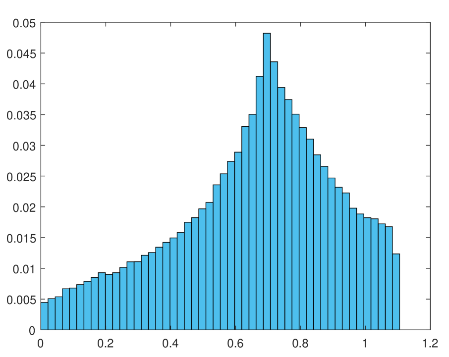
(a) prior

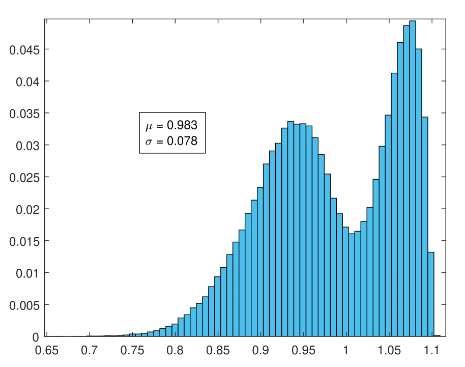
(b) $n=100$

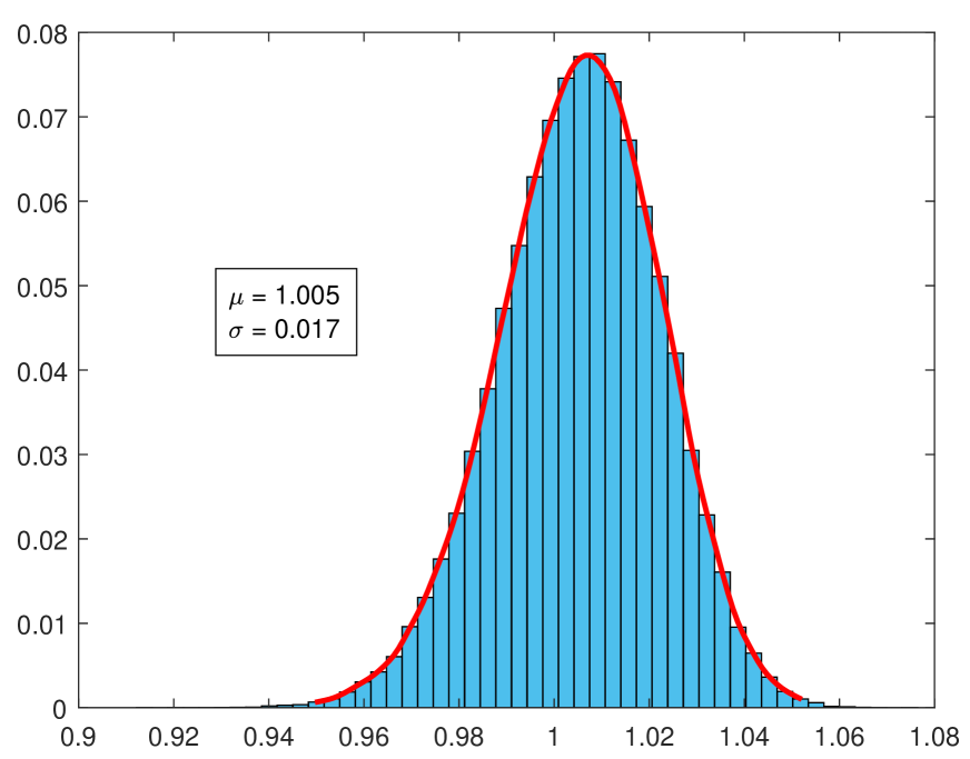
(c) $n=1000$

Figure 4: Prior $\pi(\bar{H})$ and posterior $\pi(\bar{H}|x)$ of the entropy rate $\bar{H}$ with $n=100$ and $n=1000$ observations $x$.

Figure 5 shows the performance of the BCT estimator compared with the other four estimators described above, as a function of the length $n$ of the available observations $x$. For BCT we plot the posterior mean. For the plug-in we plot estimates with block-lengths $k=5,6,7$. It is easily observed that the BCT estimator outperforms all the alternatives, and converges faster and closer to the true value of $\bar{H}$.

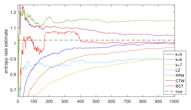
Figure 5: Entropy rate estimates for the 5th order ternary chain, as the number of observations increases.

A third order binary chain. Here, we consider $n=1000$ observations generated from an example of a third order binary chain from Berchtold and Raftery (2002). The underlying model is the complete binary tree of depth $3$ pruned at node $s=11$; the tree model $T$ and the parameter values $\theta=\{\theta_{s};s\in T\}$ are given in Section C of the supplementary material. The entropy rate of this chain is $\bar{H}=0.4815$. Figure 6 shows the performance of all five estimators, where the BCT estimator (which uses the posterior mean again) is found to have the best performance. The histogram of the BCT posterior after $n=1000$ observations, shown in Section C of the supplementary material, is close to a Gaussian with a mean $\mu=0.4806$ and a standard deviation $\sigma=0.0405$.

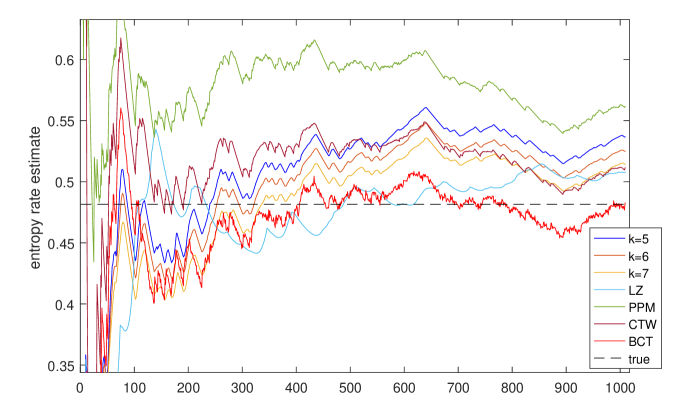
Figure 6: Entropy rate estimates for the third order binary chain, as the number of observations increases.

A bimodal posterior. We re-examine a simulated time series $x$ from Kontoyiannis et al. (2022), which consists of $n=1450$ observations generated from a $3$rd order chain $\{X_{n}\}$ with alphabet size $m=6$ and with the property that each $X_{n}$ depends on past observations only via $X_{n-3}$. The complete specification of the chain is given in Section C of the supplementary material. Its entropy rate is $\bar{H}=1.355$. An interesting aspect of this data set is that the model posterior is bimodal, with one mode corresponding to the empty tree (describing i.i.d. observations) and the other consisting of tree models of depth 3.

As shown in Figure 7(a), the posterior of the entropy rate is also bimodal here, with two separated approximately-Gaussian modes corresponding to each of the modes of the model posterior. The dominant mode is the one corresponding to models of depth 3; it has mean $\mu_{1}=1.406$, standard deviation $\sigma_{1}=0.031$, and relative weight $w_{1}=0.91$. The second mode corresponding to the empty tree has mean $\mu_{2}=1.632$, standard deviation $\sigma_{2}=0.020$, and a much smaller weight $w_{2}=1-w_{1}=0.09$. In this case, the mode of $\pi(\bar{H}|x)$ gives a more reasonable choice for a point estimate than the posterior mean. Like in the previous two examples, the BCT entropy estimator performs better than most benchmarks, as illustrated in Section C of the supplementary material.

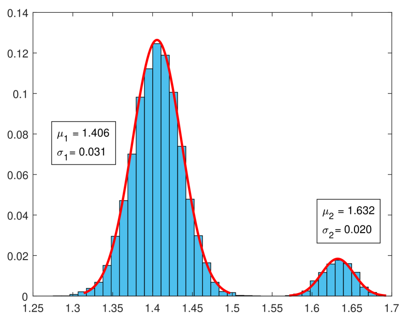
(a) bimodal example

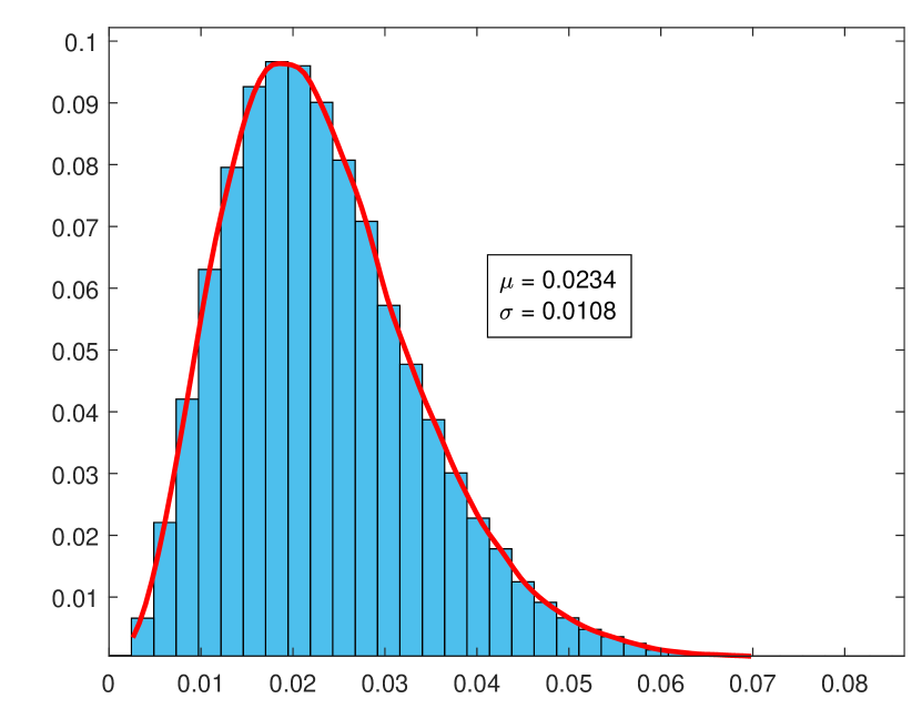
(b) spike train

Figure 7: Histograms of the posterior distribution $\pi(\bar{H}|x)$ of the entropy rate, constructed from $N=10^{5}$ i.i.d. samples in each case.

Neural spike trains. We consider $n=1000$ binary observations from a spike train recorded from a single neuron in region V4 of a monkey’s brain. The BCT posterior is shown in Figure 7(b): Its mean is $\mu=0.0234$, its standard deviation is $\sigma=0.0108$, and is skewed to the right. This dataset is the first part of a long spike train of length $n=3,919,361$ from Gregoriou et al. (2009, 2012). Although there is no “true” value of the entropy rate here, for the purposes of comparison we use the estimate obtained by the CTW estimator (identified as the most effective method by Gao et al. (2008) and Verdú (2019)) when all $n=3,919,361$ samples are used, giving $\bar{H}=0.0241$. The resulting estimates for all five methods (with the posterior mean given for BCT) are summarised in Table 1, verifying again that BCT outperforms all the other methods.

	“True”	BCT	CTW	PPM	LZ	$k=2$	$k=5$	$k=10$	$k=15$
$\widehat{H}$	0.0241	0.0234	0.0249	0.0360	0.0559	0.0204	0.0204	0.0198	0.0187

Table 1: Entropy rate estimates for the neural spike train.

Financial data. Here, we consider $n=2000$ observations from the financial dataset F.2 of Kontoyiannis et al. (2022). This consists of tick-by-tick price changes of the Facebook stock price, quantised to three values: $x_{i}=0$ if the price goes down, $x_{i}=1$ if it stays the same, and $x_{i}=2$ if it goes up. The BCT entropy-rate posterior is shown in Figure 8(a): It has mean $\mu=0.921$, and standard deviation $\sigma=0.028$.

Once again, as the “true” value of the entropy rate we take the estimate produced by the CTW estimator on a longer sequence with $n=10^{4}$ observations, giving $\bar{H}=0.916$. The results of all five estimators are summarised in Table 2, where for the BCT estimator we once again give the posterior mean.

	“True”	BCT	CTW	PPM	LZ	$k=5$	$k=6$	$k=7$	$k=10$
$\widehat{H}$	0.916	0.921	0.939	1.049	0.846	0.930	0.907	0.870	0.713

Table 2: Entropy rate estimates for the financial data set.

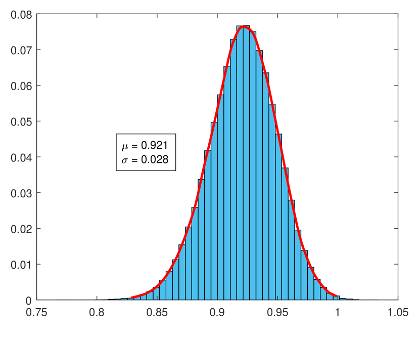
(a) financial dataset

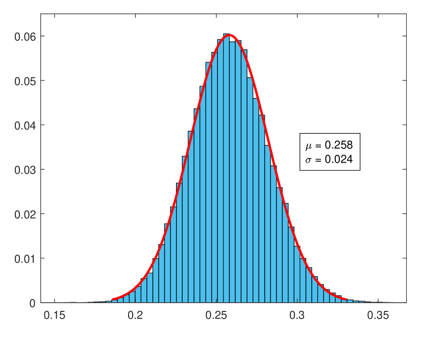
(b) pewee birdsong

Figure 8: Histograms of the posterior distribution $\pi(\bar{H}|x)$ of the entropy rate, constructed from $N=10^{5}$ i.i.d. samples in each case.

Pewee birdsong. The last data set examined is a time series $x$ describing the twilight song of the wood pewee bird (Craig, 1943; Sarkar and Dunson, 2016). It consists of $n=1327$ observations from an alphabet of size $m=3$. The BCT posterior is shown in Figure 8(b): It is approximately Gaussian with mean $\mu=0.258$ and standard deviation $\sigma=0.024$. The fact that the standard deviation is small is important as it suggests “confidence” in the resulting estimates, which is important because here (as in most real applications) there is no knowledge of a “true” underlying value. Table 3 shows all the resulting estimates; the posterior mean is shown for the BCT estimator.

	BCT	CTW	PPM	LZ	$k=2$	$k=5$	$k=10$	$k=15$
$\widehat{H}$	0.258	0.278	0.318	0.275	0.776	0.467	0.336	0.272

Table 3: Entropy rate estimates for the pewee song data.

Summary. The main conclusion from the results on the six data sets examined in this section is that the BCT estimator gives the most accurate and reliable results among the five estimators considered. In addition to the fact that the BCT point estimates typically outperform those produced by other methods, the BCT estimator is accompanied by the entire posterior distribution $\pi(\bar{H}|x)$ of the entropy rate, induced by the observations $x$. As usual, this distribution can be used to quantify the uncertainty in estimating $\bar{H}$, and it contains significantly more information than simple point estimates and their associated confidence intervals.

6 Concluding remarks

In this work, we revisited the Bayesian Context Trees (BCT) modelling framework, which was recently found to be very effective for a range of statistical tasks in the analysis of discrete time series. We showed that the prior and posterior distributions on model space admit simple and easily interpretable representations in terms of branching processes, and we demonstrated their utility both in theory and in practice.

The branching process representation was first employed to develop an efficient Monte Carlo sampler that provides i.i.d. samples from the joint posterior on models and parameters, thus facilitating effective Bayesian inference with empirical time series data. Then, it was used to establish strong theoretical results on the asymptotic consistency of the BCT posterior on model space, which provide important theoretical justifications for the use of the BCT framework in practice. Finally, the performance of the proposed Monte Carlo sampler was examined extensively in the context of entropy estimation. The resulting fully-Bayesian entropy estimator was found to outperform several of the state-of-the-art approaches, on simulated and real-world data.

Although the BCT framework was originally developed for modelling and inference of discrete-valued time series, it was recently used to develop general mixture models for real-valued time series, along with a collection of associated algorithmic tools for inference (Papageorgiou and Kontoyiannis, 2022a). Extending the results presented in this work to that setting presents an interesting direction of further research, motivated by important practical applications.

Appendix A Proof of Proposition 3.2

We need the following representation of the marginal likelihood from (Kontoyiannis et al., 2022).

Lemma A.1.

The marginal likelihood $P(x|T)$ of the observations $x$ given a model $T$ is,

$$P(x|T)=\int P(x|\theta,T)\pi(\theta|T)d\theta=\prod_{s\in T}P_{e,s},$$

where $P_{e,s}$ are the estimated probabilities in (2.4).

Proof of Proposition 3.2. The proof parallels that of Proposition 3.1. When $D=0$, $\mathcal{T}(D)$ consists of a single tree, $T=\{\lambda\}$, which has probability 1 under both the BCT posterior $\pi(\cdot|x)$ and under the distribution $\pi_{b}(\cdot)$ induced by the branching process construction. Suppose $D\geq 1$.

As before, we view every tree $T\in\mathcal{T}(D)$ as a collection of $k$ of $m$-branches, and we proceed by induction on $k$. For $k=0$, i.e., for $T=\{\lambda\}$, by the definitions,

$$\pi_{b}(\{\lambda\})=P_{b,\lambda}=\frac{\beta P_{e,\lambda}}{P_{w,\lambda}}=\pi_{D}(\{\lambda\};\beta)\frac{P_{e,\lambda}}{P_{w,\lambda}},$$

and using Lemma A.1 and the fact that $P_{w,\lambda}$ is exactly the normalising constant $P(x)$,

$$\pi_{b}(\{\lambda\})=\frac{\pi_{D}(\{\lambda\};\beta)P(x|\{\lambda\})}{P(x)}=\pi(\{\lambda\}|x).$$

Now assume the result of the proposition holds for all trees with $k$ $m$-branches, and suppose $T^{\prime}\in\mathcal{T}(D)$ contains $(k+1)$ $m$-branches and is obtained from some $T\in\mathcal{T}(D)$ by adding a single $m$-branch to one of its leaves, $s$. Again, consider two cases.

$(i)$ If $s$ is at depth $D-2$ or smaller, then by construction,

$$\pi_{b}(T^{\prime})= \frac{\pi_{b}(T)}{P_{b,s}}(1-P_{b,s})\prod_{j=0}^{m-1}P_{b,sj},$$

and therefore, using the inductive hypothesis,

$$\pi_{b}(T^{\prime})=\pi(T|x)\Big{(}\frac{1-P_{b,s}}{P_{b,s}}\Big{)}\prod_{j}P_{b,sj}=\pi(T^{\prime}|x)\frac{\pi(T|x)}{\pi(T^{\prime}|x)}\Big{(}\frac{1-P_{b,s}}{P_{b,s}}\Big{)}\prod_{j}P_{b,sj}.$$ (A.1)

Using the definitions of $\pi_{D}$ and $P_{b,s}$, as well as Lemma A.1, we can express the posterior odds $\frac{\pi(T^{\prime}|x)}{\pi(T|x)}$ in (A.1) as,

$$\frac{\pi_{D}(T^{\prime};\beta)}{\pi_{D}(T;\beta)}\frac{P(x|T^{\prime})}{P(x|T)}= \frac{\pi_{D}(T^{\prime};\beta)}{\pi_{D}(T;\beta)}\frac{\prod_{j=0}^{m-1}P_{e,sj}}{P_{e,s}}$$

$$= \frac{\beta^{m}(1-\beta)}{\beta}\frac{\prod_{j}P_{e,sj}}{P_{e,s}}$$

$$= (1-P_{b,s})\frac{1-\beta}{\beta P_{e,s}(1-P_{b,s})}\prod_{j}\beta P_{e,sj}$$

$$= (1-P_{b,s})\frac{P_{w,s}}{\beta P_{e,s}}\frac{1-\beta}{(P_{w,s}-\beta P_{e,s})}\prod_{j}\beta P_{e,sj},$$

and from the definitions of $P_{w,s}$ and $P_{b,s}$ we obtain,

$$\frac{\pi(T^{\prime}|x)}{\pi(T|x)}=(1-P_{b,s})\frac{1}{P_{b,s}}\frac{1}{\prod_{j}P_{w,sj}}\prod_{j}\beta P_{e,sj}=\Big{(}\frac{1-P_{b,s}}{P_{b,s}}\Big{)}\prod_{j}P_{b,sj}.$$ (A.2)

Substituting (A.2) into (A.1) yields, $\pi_{b}(T^{\prime})=\pi(T^{\prime}|x)$, as claimed.

$(ii)$ Similarly, if $s$ is at depth $D-1$, from the inductive hypothesis,

$$\pi_{b}(T^{\prime})=\frac{\pi_{b}(T)}{P_{b,s}}(1-P_{b,s})=\pi(T|x)\Big{(}\frac{1-P_{b,s}}{P_{b,s}}\Big{)}=\pi(T^{\prime}|x)\frac{\pi(T|x)}{\pi(T^{\prime}|x)}\Big{(}\frac{1-P_{b,s}}{P_{b,s}}\Big{)},$$

where the posterior odds can be expressed as,

$$\frac{\pi(T^{\prime}|x)}{\pi(T|x)}= \frac{\pi_{D}(T^{\prime};\beta)}{\pi_{D}(T;\beta)}\frac{\prod_{j=0}^{m-1}P_{e,sj}}{P_{e,s}}$$

$$= \Big{(}\frac{1-\beta}{\beta}\Big{)}\frac{\prod_{j}P_{w,sj}}{P_{e,s}}$$

$$= \frac{P_{w,s}-\beta P_{e,s}}{\beta P_{e,s}}=\frac{1-P_{b,s}}{P_{b,s}},$$ (A.3)

where in the second equality we used that $P_{w,sj}=P_{e,sj}$, as all nodes $sj$ are at depth $d=D$ in this case. Substituting (A) above yields $\pi_{b}(T^{\prime})=\pi(T^{\prime}|x)$, and completes the proof.     $\Box$

Appendix B Proofs of results from Section 4

B.1 Proof of Lemma 4.2

Here we establish the two missing steps in the proof of the lemma given in Section 4.1 of the main text.

Proof of (4.5). Using the upper bound of Lemma 4.1 for a fixed context $s$, and the corresponding lower bound for the context $sj$, we obtain the upper bound,

$$\frac{1}{M_{s}}\left(\log P_{e,s}-\sum_{j=0}^{m-1}\log P_{e,sj}\right)\leq \sum_{i=0}^{m-1}\frac{a_{s}(i)}{M_{s}}\log\frac{a_{s}(i)}{M_{s}}-\sum_{j=0}^{m-1}\frac{M_{sj}}{M_{s}}\sum_{i=0}^{m-1}\frac{a_{sj}(i)}{M_{sj}}\log\frac{a_{sj}(i)}{M_{sj}}$$

$$+ \frac{m-1}{2M_{s}}\left(\sum_{j=0}^{m-1}\log M_{sj}-\log M_{s}\right)+\frac{C}{M_{s}},$$ (B.1)

for some constant $C$. Since $M_{s}$ and $M_{sj}$ both tend to infinity a.s. as $n\to\infty$ by positive-ergodicity, the last two terms above both vanish a.s.

For the first two terms, we first note that, by the ergodic theorem for Markov chains (e.g., (Chung, 1967, p. 92)),

$$\frac{a_{s}(i)}{M_{s}}=\frac{a_{s}(i)}{n}\ \frac{n}{M_{s}}\to\frac{\pi(si)}{\pi(s)}=\pi(i|s),\quad\text{a.s.},$$ (B.2)

where for the stationary distribution $\pi$, the notation we use is that $si$ denotes the concatenation of context $s$ followed by symbol $i$ moving ‘forward’ in time.

Recalling the definition of $X$ and $J$, we have,

$$\mathbb{P}(X=i|s)=\frac{\pi(si)}{\pi(s)}=\pi(i|s),\quad\mathbb{P}(J=j|s)=\frac{\pi(js)}{\pi(s)},$$ (B.3)

so that for the first term of (B.1), as $n\to\infty$,

$$\sum_{i=0}^{m-1}\frac{a_{s}(i)}{M_{s}}\log\frac{a_{s}(i)}{M_{s}}\to-H(X|s),\quad\text{a.s.}$$ (B.4)

Similarly, for the second term of (B.1), from the ergodic theorem,

$$\frac{a_{sj}(i)}{M_{sj}}=\frac{a_{sj}(i)}{n}\ \frac{n}{M_{sj}}\to\frac{\pi(jsi)}{\pi(js)}=\pi(i|js)=\mathbb{P}(X=i|s,J=j),\quad\text{a.s.},$$ (B.5)

$$\frac{M_{sj}}{M_{s}}=\frac{M_{sj}}{n}\ \frac{n}{M_{s}}\to\frac{\pi(js)}{\pi(s)}=\mathbb{P}(J=j|s),\quad\text{a.s.},$$ (B.6)

so that, as $n\to\infty$,

$$-\sum_{j=0}^{m-1}\frac{M_{sj}}{M_{s}}\sum_{i=0}^{m-1}\frac{a_{sj}(i)}{M_{sj}}\log\frac{a_{sj}(i)}{M_{sj}}\to\sum_{j=0}^{m-1}\mathbb{P}(J=j|s)H(X|s,J=j)=H(X|s,J),$$ (B.7)

by the definition of conditional entropy. Finally, combining with (B.4), we get,

$$\sum_{i=0}^{m-1}\frac{a_{s}(i)}{M_{s}}\log\frac{a_{s}(i)}{M_{s}}-\sum_{j=0}^{m-1}\frac{M_{sj}}{M_{s}}\sum_{i=0}^{m-1}\frac{a_{sj}(i)}{M_{sj}}\log\frac{a_{sj}(i)}{M_{sj}}\to-I(X;J|s),\quad\text{a.s.}$$ (B.8)

Following the same sequence of steps, we can obtain a lower bound corresponding to (B.1) as,

$$\frac{1}{M_{s}}\left(\log P_{e,s}-\sum_{j=0}^{m-1}\log P_{e,sj}\right)\geq \sum_{i=0}^{m-1}\frac{a_{s}(i)}{M_{s}}\log\frac{a_{s}(i)}{M_{s}}-\sum_{j=0}^{m-1}\frac{M_{sj}}{M_{s}}\sum_{i=0}^{m-1}\frac{a_{sj}(i)}{M_{sj}}\log\frac{a_{sj}(i)}{M_{sj}}$$

$$+ \frac{m-1}{2M_{s}}\left(\sum_{j=0}^{m-1}\log M_{sj}-\log M_{s}\right)+\frac{C^{\prime}}{M_{s}},$$ (B.9)

where the only difference from (B.1) is the constant $C^{\prime}$. Therefore,

$$\frac{1}{M_{s}}\left(\log P_{e,s}-\sum_{j=0}^{m-1}\log P_{e,sj}\right)\to-I(X;J|s),\quad\text{a.s.},$$

or, equivalently,

$$\log P_{e,s}-\sum_{j=0}^{m-1}\log P_{e,sj}=-M_{s}I(X;J|s)+o(M_{s}),\quad\text{a.s.}$$ (B.10)

And since $M_{s}=n\pi(s)+o(1)$ a.s. by the ergodic theorem, we get (4.5).     $\Box$

Proof of final step in Lemma 4.2. As already noted, (4.5) implies $P_{b,s}\to 0$ a.s. for nodes whose children are leaves of $T^{*}$. The same holds for all internal nodes $s$ of $T^{*}$ for which $I(X;J|s)>0$. The only remaining case is that of internal nodes $u$ for which $I(X;J|u)=0$. The fact that again $P_{b,u}\to 0$ a.s. is an immediate consequence of the result given as Lemma B.1 in Section B.3.     $\Box$

B.2 Proof of Lemma 4.3

Here we provide proofs for the two missing steps in the proof of the lemma given in Section 4.1 of the main text.

Proof of (4.6). We can rewrite (B.9) as,

$$\sum_{j=0}^{m-1}\log P_{e,sj}-\log P_{e,s} \leq\sum_{j=0}^{m-1}\sum_{i=0}^{m-1}{a_{sj}(i)}\log\frac{a_{sj}(i)}{M_{sj}}-\sum_{i=0}^{m-1}{a_{s}(i)}\log\frac{a_{s}(i)}{M_{s}}$$

$$-\frac{m-1}{2}\left(\sum_{j=0}^{m-1}\log M_{sj}-\log M_{s}\right)-{C^{\prime}}.$$ (B.11)

We write $\widehat{p}_{s}$ and $\pi_{s}$ for the empirical and stationary conditional distributions of the symbol following $s$,

$$\widehat{p}_{s}(i):=\frac{a_{s}(i)}{M_{s}},\quad\pi_{s}(i):=\pi(i|s)=\frac{\pi(si)}{\pi(s)},\qquad i\in A.$$

Let $D(p\|q)$ denote the relative entropy (or Kullback-Leibler divergence) between two probability mass functions $p,q$ on the same discrete alphabet (Cover and Thomas, 2012, Ch. 2). By the nonnegativity of relative entropy we have,

$$\sum_{i=0}^{m-1}a_{s}(i)\log\pi_{s}(i)-\sum_{i=0}^{m-1}{a_{s}(i)}\log\frac{a_{s}(i)}{M_{s}}=M_{s}\sum_{i=0}^{m-1}{\widehat{p}_{s}(i)}\log\frac{\pi_{s}(i)}{\widehat{p}_{s}(i)}=-M_{s}D(\widehat{p}_{s}\|\pi_{s})\leq 0.$$

Adding and subtracting the term $\sum_{i=0}^{m-1}a_{s}(i)\log\pi_{s}(i)$ to (B.11) and using the last inequality,

$$\sum_{j=0}^{m-1}\log P_{e,sj}-\log P_{e,s} \leq\sum_{j=0}^{m-1}\sum_{i=0}^{m-1}a_{sj}(i)\log\widehat{p}_{sj}(i)-\sum_{i=0}^{m-1}a_{s}(i)\log\pi_{s}(i)$$

$$-\frac{m-1}{2}\left(\sum_{j=0}^{m-1}\log M_{sj}-\log M_{s}\right)-{C^{\prime}}.$$ (B.12)

We examine the first and second terms in (B.12) separately. For the first (and main) term, since for all count vectors, $a_{s}(i)=\sum_{j=0}^{m-1}a_{sj}(i)$, we can express,

$$\sum_{j=0}^{m-1}\sum_{i=0}^{m-1}a_{sj}(i)\log\widehat{p}_{sj}(i)-\sum_{i=0}^{m-1}a_{s}(i)\log\pi_{s}(i)= \sum_{j=0}^{m-1}\sum_{i=0}^{m-1}a_{sj}(i)\log\frac{\widehat{p}_{sj}(i)}{\pi_{s}(i)}$$

$$= \sum_{j=0}^{m-1}M_{sj}\sum_{i=0}^{m-1}\widehat{p}_{sj}(i)\log\frac{\widehat{p}_{sj}(i)}{\pi_{s}(i)}$$

$$= \sum_{j=0}^{m-1}M_{sj}D(\widehat{p}_{sj}\|\pi_{s})$$

$$= \sum_{j=0}^{m-1}M_{sj}D(\widehat{p}_{sj}\|\pi_{sj}),$$

where the last equality holds because $s$ is either a leaf or an external nodes of $T^{*}$, so that $I(X;J|s)=0$ and $\pi_{sj}=\pi_{sj^{\prime}}=\pi_{s}$, for all $j,j^{\prime}$.

In order to bound the relative entropy between the empirical and the stationary conditional distributions, we first recall that relative entropy is bounded above by the $\chi^{2}$-distance, e.g., (Gibbs and Su, 2002),

$$D(\widehat{p}_{sj}\|\pi_{sj})\leq d_{\chi^{2}}(\widehat{p}_{sj},\pi_{sj})=\sum_{i=0}^{m-1}\frac{(\widehat{p}_{sj}(i)-\pi_{sj}(i))^{2}}{\pi_{sj}(i)}.$$ (B.13)

From the law of the iterated logarithm (LIL) for Markov chains (Chung, 1967, p. 106), we have, a.s. as $n\to\infty$,

$$a_{sj}(i)=n\pi(jsi)+O(\sqrt{n\log\log n}),\quad M_{sj}=n\pi(js)+O(\sqrt{n\log\log n}),$$ (B.14)

so that,

$$\widehat{p}_{sj}(i)=\frac{a_{sj}(i)}{M_{sj}}=\frac{\pi(jsi)}{\pi(js)}+O\left(\sqrt{\frac{\log\log n}{n}}\right)=\pi_{sj}(i)+O\left(\sqrt{\frac{\log\log n}{n}}\right).$$

Substituting in (B.13) yields,

$$D(\widehat{p}_{sj}\|\pi_{sj})\leq O\left({\frac{\log\log n}{n}}\right)\sum_{i=0}^{m-1}\frac{1}{\pi_{sj}(i)}=O\left({\frac{\log\log n}{n}}\right),\quad\text{a.s.},$$ (B.15)

and finally, using (B.14) again,

$$\sum_{j=0}^{m-1}M_{sj}D(\widehat{p}_{sj}\|\pi_{sj})=O(\log\log n),\quad\text{a.s.}$$ (B.16)

For the third term in (B.12),

$$\sum_{j=0}^{m-1}\log M_{sj}-\log M_{s}=\sum_{j=0}^{m-1}\log\frac{M_{sj}}{M_{s}}+(m-1)\log M_{s}.$$

Using the LIL, $M_{s}=n\pi(s)+O(\sqrt{n\log\log n})$, a.s., so,

$$\log M_{s}=\log\left(n\pi(s)\left\{1+O(\sqrt{\log\log n/n})\right\}\right)=\log n+O(1),\quad\text{a.s.}$$

And, using LIL again as above, $M_{sj}/M_{s}=\pi(js)/\pi(s)+O(\sqrt{\log\log n/n})=O(1)$, a.s., so that, $\log{M_{sj}}/{M_{s}}=O(1)$, a.s., and,

$$\sum_{j=0}^{m-1}\log M_{sj}-\log M_{s}=(m-1)\log n+O(1),\quad\text{a.s.},$$ (B.17)

which together with (B.12) and (B.16) complete the proof of equation (4.6).     $\Box$

Proof of final step in Lemma 4.3. As discussed in the proof of Lemma 4.3 in the main text, the asymptotic relation (4.6) implies that $\prod_{j}P_{e,sj}/{P_{e,s}}\to 0$, a.s., for all leaves and external nodes $s$ of $T^{*}$. The next proposition states that it also implies that $\prod_{j}P_{w,sj}/{P_{e,s}}\to 0$, so that by (4.3) $P_{b,s}\to 1$, a.s., completing the proof of Lemma 4.3. Note that it suffices to consider leaves at depths $d\leq D-1$, since for leaves $s$ at depth $D$ we already have $P_{b,s}=1$.     $\Box$

Proposition B.1.

Under the assumptions of Theorem 4.1, for all leaves and external nodes $s$ of $T^{*}$ at depths $d\leq D-1$ we have, as $n\to\infty$:

$$\frac{\prod_{j=0}^{m-1}P_{w,sj}}{{P_{e,s}}}\to 0,\quad\text{a.s.}$$

Proof. Note that, since the stationary distribution is positive on all finite contexts, the tree $T_{\text{MAX}}$ is eventually a.s. the complete tree of depth $D$, so we need not consider special cases of contexts $s$ that do not appear in the data separately. Let $s$ be a leaf or external node of $T^{*}$ at depth $0\leq d\leq D-1$. The proof is by induction on $d$.

For $d=D-1$, the claim is satisfied trivially as $P_{w,sj}=P_{e,sj}$, since nodes $sj$ are at depth $D$. For the inductive step, we assume that the claim holds for all leaves and external nodes $s$ of $T^{*}$ at some depth $d\leq D-1$, and consider a leaf or external node $s$ of $T^{*}$ at depth $d-1$. We have, as $n\to\infty$,

$$\frac{\prod_{j=0}^{m-1}P_{w,sj}}{{P_{e,s}}}= \frac{\prod_{j=0}^{m-1}\big{[}\beta P_{e,sj}+(1-\beta)\prod_{t=0}^{m-1}P_{w,sjt}\big{]}}{{P_{e,s}}}$$

$$= \frac{\prod_{j=0}^{m-1}\big{[}\beta P_{e,sj}+(1-\beta)\prod_{t=0}^{m-1}P_{w,sjt}\big{]}}{\prod_{j=0}^{m-1}\beta P_{e,sj}}\ \frac{\prod_{j=0}^{m-1}\beta P_{e,sj}}{{P_{e,s}}}$$

$$= \prod_{j=0}^{m-1}\left(1+\frac{1-\beta}{\beta}\frac{\prod_{t=0}^{m-1}P_{w,sjt}}{P_{e,sj}}\right)\ \frac{\prod_{j=0}^{m-1}P_{e,sj}}{{P_{e,s}}}\beta^{m}\to 0,\quad\text{a.s.},$$ (B.18)

as ${\prod_{t=0}^{m-1}P_{w,sjt}}/{P_{e,sj}}\to 0$ by the inductive hypothesis, and ${\prod_{j=0}^{m-1}P_{e,sj}}/{{P_{e,s}}}\to 0$ for a node $s$ which is either a leaf or external node of $T^{*}$. This establishes the inductive step and completes the proof.     $\Box$

B.3 Proof of Theorem 4.2

The starting point of the proof is the representation of the posterior given in equation (3.2) of the main text. In particular, we examine the asymptotic behaviour of the branching probabilities $P_{b,s}$ separately for leaves and internal nodes.

Leaves. Let $s$ be a leaf or an external node of $T^{*}$. We already have a strong upper bound for the estimated probabilities of $s$ in (4.6). Write $r=(m-1)^{2}/2$. Since the bound (4.6) holds a.s., a straightforward sample-path-wise computation immediately implies that, for all $\epsilon>0$,

$$\frac{\prod_{j=0}^{m-1}P_{e,sj}}{P_{e,s}}=O\big{(}n^{-r+\epsilon}\big{)},\quad\text{a.s.}$$ (B.19)

Proposition B.2 states that $\prod_{j}P_{w,sj}/{P_{e,s}}$ has the same asymptotic behaviour.

Proposition B.2.

For all leaves and external nodes $s$ of $T^{*}$ at depths $d\leq D-1$, for any $\epsilon>0$ we have as $n\to\infty$:

$$\frac{\prod_{j=0}^{m-1}P_{w,sj}}{{P_{e,s}}}={O}\left(n^{-\frac{(m-1)^{2}}{2}+\epsilon}\right),\quad\text{a.s.}$$

Proof. The proof is similar to that of Proposition B.1, by induction on $d$.

If $d=D-1$, then $P_{w,sj}=P_{e,sj}$ and the claim follows from (B.19). For the inductive step, assume the claim holds for all leaves and external nodes at some depth $d\leq D-1$, and consider a leaf or external node $s$ at depth $d-1$. Then substituting (B.19) into (B.18) and noting that ${\prod_{t}P_{w,sjt}}/{P_{e,sj}}\to 0$ a.s. by Proposition B.1, completes the proof.     $\Box$

Combining Proposition B.2 with equation (4.3), we get that, for any leaf or external node $s$ at depth $d$, a.s. as $n\to\infty$:

$$P_{b,s}=1-{O}\left(n^{-\frac{(m-1)^{2}}{2}+\epsilon}\right),\quad\mbox{if }d\leq D-1,\qquad\mbox{and }P_{b,s}=1,\quad\mbox{if }d=D.$$ (B.20)

Internal nodes. As in the proof of Lemma 4.2, we first consider internal nodes whose children are leaves of $T^{*}$, so that $I=I(X;J|s)>0$. For these nodes, equation (4.5) gives,

$$\frac{P_{e,s}}{\prod_{j=0}^{m-1}P_{e,sj}}=\exp\big{\{}-nI\pi(s)+o(n)\big{\}},\quad\text{a.s.},$$ (B.21)

so for any $\epsilon>0$,

$$\frac{P_{e,s}}{\prod_{j=0}^{m-1}P_{e,sj}}=o\big{(}\exp\big{\{}-n(1-\epsilon)I\pi(s)\big{\}}\big{)},\quad\text{a.s.},$$ (B.22)

and substituting in equation (4.4) in the main text we obtain the same bound for the branching probabilities,

$$P_{b,s}=o\Big{(}\exp\big{\{}-n(1-\epsilon)I\pi(s)\big{\}}\Big{)},\quad\text{a.s.}$$ (B.23)

Next we establish a corresponding bound for all internal nodes, indeed, for any node $u$ that is a suffix of a node $s$ that has $I(X;J|s)>0$.

Lemma B.1.

Let $s$ be a context of length $l(s)\leq D-1$ for which $I(X;J|s)>0$, and let $u$ be any suffix of $s$. Then, for any $\epsilon>0$, we have as $n\to\infty$:

$$P_{b,u}=o\Big{(}\exp\big{\{}-n(1-\epsilon)I(X;J|s)\pi(s)\big{\}}\Big{)},\quad\text{a.s.}$$ (B.24)

Proof. Let $\Delta l=l(s)-l(u)\geq 0$; the proof is by induction on $\Delta l$. For $\Delta l=0$, the claim is satisfied trivially as $u=s$, for which $I(X;J|s)>0$, corresponding to the previous case.

For the inductive step, we assume that the claim holds for context $uj$ which is the suffix of $s$ with $\Delta l=k\geq 0$, and prove that it also holds for the context $u$, which is the suffix of $s$ with $\Delta l=k+1$. For node $u$, which is at depth $d<D-1$, from (4.4) and the definition of the branching probabilities,

$$P_{b,u}\leq\Big{(}\frac{\beta}{1-\beta}\Big{)}\frac{P_{e,u}}{\prod_{t=0}^{m-1}P_{w,ut}}=C\frac{P_{e,u}}{\prod_{t=0}^{m-1}P_{e,ut}}\prod_{t=0}^{m-1}P_{b,ut},$$

where the constant $C=[\beta^{m-1}(1-\beta)]^{-1}$. And, as $P_{b,ut}\leq 1$ for all $t$, we can further bound,

$$P_{b,u}\leq C\ \frac{P_{e,u}}{\prod_{t=0}^{m-1}P_{e,ut}}\ P_{b,uj},$$ (B.25)

keeping only the specific child $uj$ of $u$ which is a suffix of $s$.

From (B.21) for node $u$, we know that, even if $I(X;J|u)$ is zero, we have,

$$\frac{P_{e,u}}{\prod_{t=0}^{m-1}P_{e,ut}}=\exp(o(n)),\quad\text{a.s.},$$ (B.26)

and combining this with (B.25) and the inductive hypothesis that (B.24) holds for $uj$ in place of $u$,

$$P_{b,u}=o\Big{(}\exp\big{\{}-n(1-2\epsilon)I(X;J|s)\pi(s)\big{\}}\Big{)},\quad\text{a.s.},$$

completing the proof of the inductive step and the proof of the lemma.     $\Box$

Substituting the bounds on the branching probabilities on the leaves (B.20) and on the internal nodes (B.24) into the expression for the posterior of $T^{*}$ in equation (3.2) in the main text, yields the result claimed in Theorem 4.2. Finally, a simple examination of (B.20) and (B.24) in the case when $T^{*}$ is the full tree of depth $D$ shows that $P_{b,s}=1$ for all leaves $s$, so the rate is determined by the exponential bounds in (B.24) as claimed in Corollary 4.1.

Appendix C Entropy estimation

This section contains additional details associated with the entropy estimation experiments of Section 5.2 of the main text.

A ternary chain. The parameters of this chain are:

$$\theta_{1}=(0.4,0.4,0.2),\;\theta_{2}=(0.2,0.4,0.4),$$

$$\theta_{00}=(0.4,0.2,0.4),\;\theta_{01}=(0.3,0.6,0.1),$$

$$\theta_{022}=(0.5,0.3,0.2),$$

$$\theta_{0212}=(0.1,0.3,0.6),\;\theta_{0211}=(0.05,0.25,0.7),\;\theta_{0210}=(0.35,0.55,0.1),$$

$$\theta_{0202}=(0.1,0.2,0.7),\;\theta_{0201}=(0.8,0.05,0.15),$$

$$\theta_{02002}=(0.7,0.2,0.1),\;\theta_{02001}=(0.1,0.1,0.8),\;\theta_{02000}=(0.3,0.45,0.25).$$

A third order binary chain.

(a) tree model and parameters

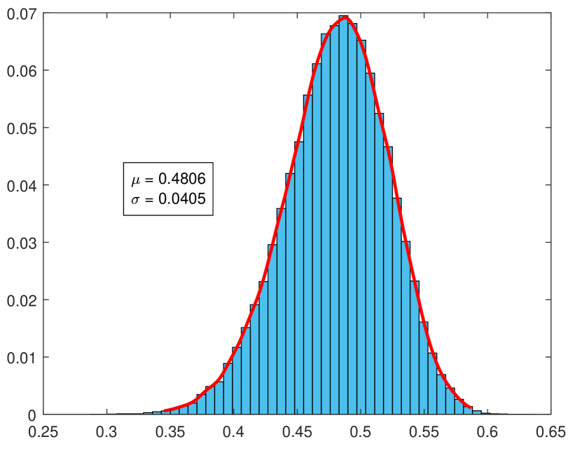
(b) entropy rate posterior

Figure 9: $(a)$ Model and parameters for the third order binary chain. $(b)$ Histogram of the posterior $\pi(\bar{H}|x)$ of the entropy rate given $n=1000$ observations from the chain, constructed from $N=10^{5}$ Monte Carlo samples.

The tree model for the third order binary chain, along with its associated parameters, is shown in Figure 9(a). The posterior $\pi(\bar{H}|x)$ of the entropy rate based on $n=1000$ observations $x$ is shown in Figure 9(b): It is approximately Gaussian with mean $\mu=0.4806$ and standard deviation $\sigma=0.0405$. The histogram was constructed using $N=10^{5}$ i.i.d. samples from the entropy rate posterior.

A bimodal posterior. The distribution of the third-order chain $\{X_{n}\}$ in this example is given by,

$$\Pr(X_{n}=j|X_{n-1}=a,X_{n-2}=b,X_{n-3}=i)=Q_{ij},\quad i,j,a,b\in A,$$

where the alphabet $A=\{0,1,2,3,4,5\}$ and the transition matrix $Q=(Q_{ij})$ is,

$$Q=\left(\begin{array}[]{cccccc}0.5&0.2&0.1&0&0.05&0.15\\ 0.4&0&0.4&0.2&0&0\\ 0.3&0.1&0.23&0.12&0.05&0.2\\ 0.05&0.1&0.05&0.05&0.03&0.72\\ 0&0&1&0&0&0\\ 0.1&0.2&0.3&0.2&0.05&0.15\end{array}\right).$$

Viewed as a variable-memory chain, the model of $\{X_{n}\}$ is the complete tree of depth 3, but the dependence of each $X_{n}$ on its past is only via $X_{n-3}$. So, meaningful dependence is detected only at memory lengths of at least three: the two most recent symbols are independent of $X_{n}$. This is why the MAP model $T_{1}^{*}$ identified by the BCT algorithm of Kontoyiannis et al. (2022) based on the $n=1450$ observations $x$ is the empty tree $T_{1}^{*}=\{\lambda\}$, corresponding to i.i.d. data. Its posterior probability is $\pi(T_{1}^{*}|x)=0.09$, which corresponds exactly to the weight of the secondary mode in the entropy rate posterior, as shown in Figure 7a of the main text. All other trees identified by the $k$-BCT algorithm are complex trees of depth 3, with posterior probabilities close to that of $T_{1}^{*}$; e.g., the second a posteriori most likely model $T_{2}^{*}$ has posterior $\pi(T_{2}^{*}|x)=0.08$. These trees of depth 3 form the other mode of the bimodal posterior on model space, which corresponds to the primary mode of the entropy rate posterior in Figure 7a.

Table 4 shows the entropy rate estimates by all five methods in this example. The MAP value of the posterior $\pi(\bar{H}|x)$ is given for BCT. Note that, although the plug-in estimator with block-length $k=5$ gives a slightly better estimate than the BCT here, given the well-known high variability of the plug-in this is likely more a coincidence rather than an indication of accuracy of the plug-in.

	True	BCT	CTW	PPM	LZ	$k=3$	$k=4$	$k=5$	$k=6$
$\widehat{H}$	1.355	1.406	1.643	1.650	1.283	1.609	1.481	1.333	1.173

Table 4: Entropy rate estimates for the ‘bimodal posterior’ example.

References

- Athreya and Ney (2004) K.B. Athreya and P.E. Ney. Branching processes. Courier Corporation, 2004.
- Bacallado (2011) S. Bacallado. Bayesian analysis of variable-order, reversible Markov chains. The Annals of Statistics, 39(2):838–864, 2011.
- Bacallado et al. (2013) S. Bacallado, S. Favaro, and L. Trippa. Bayesian nonparametric analysis of reversible Markov chains. The Annals of Statistics, pages 870–896, 2013.
- Bacallado et al. (2016) S. Bacallado, V. Pande, S. Favaro, and L. Trippa. Bayesian regularization of the length of memory in reversible sequences. Journal of the Royal Statistical Society: Series B (Statistical Methodology), 78(4):933–946, 2016.
- Berchtold and Raftery (2002) A. Berchtold and A.E. Raftery. The mixture transition distribution model for high-order markov chains and non-gaussian time series. Statistical Science, 17(3):328–356, 2002.
- Bernardo and Smith (2009) J.M. Bernardo and A.F.M. Smith. Bayesian theory, volume 405. John Wiley & Sons, 2009.
- Blackwell (1947) D. Blackwell. Conditional expectation and unbiased sequential estimation. The Annals of Mathematical Statistics, pages 105–110, 1947.
- Breiman (1992) L. Breiman. Probability. SIAM Classics in Applied Mathematics, 7, Philadelphia, PA, 1992.
- Bühlmann (2000) P. Bühlmann. Model selection for variable length Markov chains and tuning the context algorithm. Annals of the Institute of Statistical Mathematics, 52(2):287–315, 2000.
- Bühlmann and Wyner (1999) P. Bühlmann and A.J. Wyner. Variable length Markov chains. The Annals of Statistics, 27(2):480–513, 1999.
- Bunton (1996) S. Bunton. On-line stochastic processes in data compression. Ph.D. thesis, University of Washington, 1996.
- Cai et al. (2004) H. Cai, S.R. Kulkarni, and S. Verdú. Universal entropy estimation via block sorting. IEEE Transactions on Information Theory, 50(7):1551–1561, 2004.
- Catoni (2004) O. Catoni. Statistical learning theory and stochastic optimization, volume 1851 of Lecture Notes in Mathematics. Springer-Verlag, Berlin, 2004. Lecture notes from the 31st Summer School on Probability Theory held in Saint-Flour, July 8–25, 2001.
- Chipman et al. (2001) H. Chipman, E.I. George, R.E. McCulloch, M. Clyde, D.P. Foster, and R.A. Stine. The practical implementation of Bayesian model selection. In Model selection, volume 38 of IMS Lecture Notes Monogr. Ser., pages 65–134. Inst. Math. Statist., Beachwood, OH, 2001. With discussion by M. Clyde, Dean P. Foster, and Robert A. Stine, and a rejoinder by the authors.
- Chung (1967) K.L. Chung. Markov chains with stationary transition probabilities. Springer-Verlag, New York, 1967.
- Cleary and Witten (1984) J. Cleary and I. Witten. Data compression using adaptive coding and partial string matching. IEEE transactions on Communications, 32(4):396–402, 1984.
- Cover and Thomas (2012) T.M. Cover and J.A. Thomas. Elements of information theory. J. Wiley & Sons, New York, second edition, 2012.
- Cowles and Carlin (1996) M.K. Cowles and B.P. Carlin. Markov chain Monte Carlo convergence diagnostics: A comparative review. Journal of the American Statistical Association, 91(434):883–904, 1996.
- Craig (1943) W. Craig. The song of the wood pewee (Myiochanes virens Linnaeus): A study of bird music. New York State Museum Bulletin No. 334. University of the State of New York, Albany, NY, 1943.
- Csiszár and Talata (2006) I. Csiszár and Z. Talata. Context tree estimation for not necessarily finite memory processes, via BIC and MDL. IEEE Transactions on Information theory, 52(3):1007–1016, 2006.
- Feutrill and Roughan (2021) A. Feutrill and M. Roughan. A review of Shannon and differential entropy rate estimation. Entropy, 23(8), 2021.
- Fokianos and Kedem (2003) K. Fokianos and B. Kedem. Regression theory for categorical time series. Statistical Science, 18(3):357–376, 2003.
- Gao et al. (2008) Y. Gao, I. Kontoyiannis, and E. Bienenstock. Estimating the entropy of binary time series: Methodology, some theory and a simulation study. Entropy, 10(2):71–99, 2008.
- Gelfand and Smith (1990) A.E. Gelfand and A.F.M. Smith. Sampling-based approaches to calculating marginal densities. Journal of the American Statistical Association, 85(410):398–409, 1990.
- Gelman and Rubin (1992) A. Gelman and D.B. Rubin. Inference from iterative simulation using multiple sequences. Statistical Science, 7(4):457–472, 1992.
- Gelman et al. (1995) A. Gelman, J.B. Carlin, H.S. Stern, and D.B. Rubin. Bayesian data analysis. Chapman and Hall/CRC, 1995.
- Gibbs and Su (2002) A.L. Gibbs and F.E. Su. On choosing and bounding probability metrics. International Statistical Review, 70(3):419–435, 2002.
- Gregoriou et al. (2009) G.G. Gregoriou, S.J. Gotts, H. Zhou, and R. Desimone. High-frequency, long-range coupling between prefrontal and visual cortex during attention. Science, 324(5931):1207–1210, 2009.
- Gregoriou et al. (2012) G.G. Gregoriou, S.J. Gotts, and R. Desimone. Cell-type-specific synchronization of neural activity in FEF with V4 during attention. Neuron, 73(3):581–594, 2012.
- Harris (1963) T.E. Harris. The theory of branching processes, volume 6. Springer Berlin, 1963.
- Heiner and Kottas (2022) M. Heiner and A. Kottas. Estimation and selection for high-order Markov chains with Bayesian mixture transition distribution models. Journal of Computational and Graphical Statistics, 31(1):100–112, 2022.
- Heiner et al. (2019) M. Heiner, A. Kottas, and S. Munch. Structured priors for sparse probability vectors with application to model selection in Markov chains. Statistics and Computing, 29(5):1077–1093, 2019.
- Ibragimov (1962) I.A. Ibragimov. Some limit theorems for stationary processes. Theory of Probability and its Applications, 7:349–382, 1962.
- Jääskinen et al. (2014) V. Jääskinen, J. Xiong, J. Corander, and T. Koski. Sparse Markov chains for sequence data. Scandinavian Journal of Statistics, 41(3):639–655, 2014.
- Jiao et al. (2013) J. Jiao, H.H. Permuter, L. Zhao, Y.H. Kim, and T. Weissman. Universal estimation of directed information. IEEE Transactions on Information Theory, 59(10):6220–6242, 2013.
- Kershenbaum (2014) A. Kershenbaum. Entropy rate as a measure of animal vocal complexity. Bioacoustics, 23(3):195–208, 2014.
- Kontoyiannis et al. (2022) I. Kontoyiannis, L. Mertzanis, A. Panotopoulou, I. Papageorgiou, and M. Skoularidou. Bayesian Context Trees: Modelling and exact inference for discrete time series. Journal of the Royal Statistical Society: Series B (Statistical Methodology), 84(4):1287–1323, 2022.
- Krichevsky and Trofimov (1981) R. Krichevsky and V. Trofimov. The performance of universal encoding. IEEE Transactions on Information Theory, 27(2):199–207, 1981.
- London et al. (2002) M. London, A. Schreibman, M. Häusser, M.E. Larkum, and I. Segev. The information efficacy of a synapse. Nature Neuroscience, 5(4):332–340, 2002.
- Lungu et al. (2022a) V. Lungu, I. Papageorgiou, and I. Kontoyiannis. Change-point detection and segmentation of discrete data using Bayesian Context Trees. arXiv preprint arXiv:2203.04341, 2022a.
- Lungu et al. (2022b) V. Lungu, I. Papageorgiou, and I. Kontoyiannis. Bayesian change-point detection via context-tree weighting. In 2022 IEEE Information Theory Workshop (ITW), pages 125–130. IEEE, 2022b.
- Mächler and Bühlmann (2004) M. Mächler and P. Bühlmann. Variable length Markov chains: methodology, computing, and software. Journal of Computational and Graphical Statistics, 13(2):435–455, 2004.
- Meyn and Tweedie (2012) S.P. Meyn and R.L. Tweedie. Markov chains and stochastic stability. Springer Science & Business Media, 2012.
- Nemenman et al. (2004) I. Nemenman, W. Bialek, and R.R.D.R. Van Steveninck. Entropy and information in neural spike trains: Progress on the sampling problem. Physical Review E, 69(5):056111, 2004.
- Paninski (2003) L. Paninski. Estimation of entropy and mutual information. Neural Computation, 15(6):1191–1253, 2003.
- Papageorgiou and Kontoyiannis (2022a) I. Papageorgiou and I. Kontoyiannis. The Bayesian Context Trees State Space Model: Interpretable mixture models for time series. arXiv preprint arXiv:2106.03023, 2022a.
- Papageorgiou and Kontoyiannis (2022b) I. Papageorgiou and I. Kontoyiannis. The posterior distribution of Bayesian Context-Tree models: Theory and applications. In 2022 IEEE International Symposium on Information Theory (ISIT), pages 702–707. IEEE, 2022b.
- Papageorgiou and Kontoyiannis (2022c) I. Papageorgiou and I. Kontoyiannis. Truly Bayesian entropy estimation. arXiv preprint arXiv:2212.06705, 2022c.
- Papageorgiou et al. (2020) I. Papageorgiou, V.M. Lungu, and I. Kontoyiannis. BCT: Bayesian Context Trees for Discrete Time Series, 2020. R package version 1.1. https://CRAN.R-project.org/package=BCT.
- Papageorgiou et al. (2021) I. Papageorgiou, I. Kontoyiannis, L. Mertzanis, A. Panotopoulou, and M. Skoularidou. Revisiting context-tree weighting for Bayesian inference. In 2021 IEEE International Symposium on Information Theory (ISIT), pages 2906–2911, 2021.
- Philipp and Stout (1975) W. Philipp and W. Stout. Almost sure invariance principles for partial sums of weakly dependent random variables, volume 161. Memoirs of the AMS, 1975.
- Raftery (1985) A.E. Raftery. A model for high-order markov chains. Journal of the Royal Statistical Society: Series B (Methodological), 47(3):528–539, 1985.
- Rio (1995) E. Rio. The functional law of the iterated logarithm for stationary strongly mixing sequences. The Annals of Probability, pages 1188–1203, 1995.
- Rissanen (1983a) J. Rissanen. A universal data compression system. IEEE Transactions on Information Theory, 29(5):656–664, 1983a.
- Rissanen (1983b) J. Rissanen. A universal prior for integers and estimation by minimum description length. Annals of Statistics, 11(2):416–431, 1983b.
- Rissanen (1986) J. Rissanen. Complexity of strings in the class of markov sources. IEEE Transactions on Information Theory, 32(4):526–532, 1986.
- Robert and Casella (2004) C.P. Robert and G. Casella. Monte Carlo statistical methods, volume 2. Springer, 2004.
- Roy (2020) V. Roy. Convergence diagnostics for markov chain monte carlo. Annual Review of Statistics and Its Application, 7:387–412, 2020.
- Sarkar and Dunson (2016) A. Sarkar and D.B. Dunson. Bayesian nonparametric modeling of higher order Markov chains. Journal of the American Statistical Association, 111(516):1791–1803, 2016.
- Shannon (1951) C.E. Shannon. Prediction and entropy of printed English. Bell System Technical Journal, 30(1):50–64, 1951.
- Simion (2020) E. Simion. Entropy and randomness: From analogic to quantum world. IEEE Access, 8:74553–74561, 2020.
- Strong et al. (1998) S.P. Strong, R. Koberle, R.R.D.R. Van Steveninck, and W. Bialek. Entropy and information in neural spike trains. Physical Review Letters, 80(1):197, 1998.
- Timme and Lapish (2018) N.M. Timme and C. Lapish. A tutorial for information theory in neuroscience. eneuro, 5(3):1–40, 2018.
- Verdú (2019) S. Verdú. Empirical estimation of information measures: A literature guide. Entropy, 21(8):720, 2019.
- Weinberger et al. (1994) M.J. Weinberger, N. Merhav, and M. Feder. Optimal sequential probability assignment for individual sequences. IEEE Transactions on Information Theory, 40(2):384–396, 1994.
- Willems (1998) F.M.J. Willems. The context-tree weighting method: extensions. IEEE Transactions on Information Theory, 44(2):792–798, 1998.
-
Willems et al. (1993)
F.M.J. Willems, Y.M. Shtarkov, and T.J. Tjalkens.
Context tree weighting: Basic properties.
Unpublished manuscript. Available online at:
www.sps.ele.tue.nl/members/F.M.J.Willems/, August 1993. - Willems et al. (1995) F.M.J. Willems, Y.M. Shtarkov, and T.J. Tjalkens. The context-tree weighting method: basic properties. IEEE Transactions on Information Theory, 41(3):653–664, 1995.
- Willems et al. (2016) R.M. Willems, S.L. Frank, A.D. Nijhof, P. Hagoort, and A. Van den Bosch. Prediction during natural language comprehension. Cerebral Cortex, 26(6):2506–2516, 2016.
- Wyner and Ziv (1989) A.D. Wyner and J. Ziv. Some asymptotic properties of the entropy of a stationary ergodic data source with applications to data compression. IEEE Transactions on Information Theory, 35(6):1250–1258, 1989.
- Xie and Barron (2000) Q. Xie and A.R. Barron. Asymptotic minimax regret for data compression, gambling, and prediction. IEEE Transactions on Information Theory, 46(2):431–445, March 2000.
- Xiong et al. (2016) J. Xiong, V. Jääskinen, and J. Corander. Recursive learning for sparse Markov models. Bayesian Analysis, 11(1):247–263, 2016.
- Zeger and Liang (1986) S.L. Zeger and K.Y. Liang. Longitudinal data analysis for discrete and continuous outcomes. Biometrics, pages 121–130, 1986.
- Zhao and Woodroofe (2008) O. Zhao and M. Woodroofe. Law of the iterated logarithm for stationary processes. The Annals of Probability, 36(1):127–142, 2008.
- Ziv and Lempel (1977) J. Ziv and A. Lempel. A universal algorithm for sequential data compression. IEEE Transactions on Information Theory, 23(3):337–343, 1977.
Supplementary material