Covariate-Adjusted Log-Rank Test: Guaranteed Efficiency Gain and Universal Applicability

Abstract

Nonparametric covariate adjustment is considered for log-rank type tests of treatment effect with right-censored time-to-event data from clinical trials applying covariate-adaptive randomization. Our proposed covariate-adjusted log-rank test has a simple explicit formula and a guaranteed efficiency gain over the unadjusted test. We also show that our proposed test achieves universal applicability in the sense that the same formula of test can be universally applied to simple randomization and all commonly used covariate-adaptive randomization schemes such as the stratified permuted block and Pocock and Simon’s minimization, which is not a property enjoyed by the unadjusted log-rank test. Our method is supported by novel asymptotic theory and empirical results for type I error and power of tests.

Keywords: Covariate calibration; Minimization; Pitman’s relative efficiency; Permuted block; Stratification; Time-to-event data; Validity and power of tests.

1 Introduction

In clinical trials, adjusting for baseline covariates has been widely advocated as a way to improve efficiency for demonstrating treatment effects, “under approximately the same minimal statistical assumptions that would be needed for unadjusted estimation” (ICH E9,, 1998; EMA,, 2015; FDA,, 2021). In testing for effect between two treatments with right-censored time-to-event outcomes, adjusting for covariates using the Cox proportional hazards model has been demonstrated to yield valid tests even if the Cox model is misspecified (Lin and Wei,, 1989; Kong and Slud,, 1997; DiRienzo and Lagakos,, 2002). However, these tests may be less powerful than the log-rank test that does not adjust for any covariates when the Cox model is misspecified (Kong and Slud,, 1997). Although efforts have been made to improve the efficiency of the log-rank test through covariate adjustment from semiparametric theory (Lu and Tsiatis,, 2008; Moore and van der Laan,, 2009), the solutions are complicated and their validities are established only under simple randomization, i.e., treatments are assigned to patients completely at random.

To balance the number of patients in each treatment arm across baseline prognostic factors in clinical trials with sequentially arrived patients, covariate-adaptive randomization has become the new norm. From 1989 to 2008, covariate-adaptive randomization was used in more than 500 clinical trials (Taves,, 2010); among nearly 300 trials published in two years, 2009 and 2014, 237 of them applied covariate-adaptive randomization (Ciolino et al.,, 2019). The two most popular covariate-adaptive randomization schemes are the stratified permuted block (Zelen,, 1974) and Pocock-Simon’s minimization (Taves,, 1974; Pocock and Simon,, 1975). Other schemes can be found in two reviews, Schulz and Grimes, (2002) and Shao, (2021). Unlike simple randomization, covariate-adaptive randomization generates a dependent sequence of treatment assignments, which may render conventional methods developed under simple randomization not necessarily valid under covariate-adaptive randomization (EMA,, 2015; FDA,, 2021). For time-to-event data under covariate-adaptive randomization, Ye and Shao, (2020) shows that some conventional tests including the log-rank test are conservative and Wang et al., (2021) shows that the Kaplan-Meier estimator of survival function has reduced variance compared to that under simple randomization.

The discussion so far has brought up two issues in adjusting covariates, the guaranteed efficiency gain over unadjusted method under the same assumption and the wide applicability to all commonly used covariate-adaptive randomization schemes. These issues have been well addressed when adjustments are made under linear working models for non-time-to-event data (Tsiatis et al.,, 2008; Zhang et al.,, 2008; Lin,, 2013; Ye et al.,, 2022). Ye et al., (2022) also shows that adjustment via linear working models can achieve universal applicability in the sense that the same inference procedure can be universally applied to all commonly used covariate-adaptive randomization schemes, a desirable property for application. For right-censored time-to-event outcomes, to the best of our knowledge, no result has been established for covariate adjustment with guaranteed efficiency gain and universal applicability.

In this paper we propose a nonparametric covariate adjustment method for the log-rank test, which has a simple explicit form and can achieve the goal of guaranteed efficiency gain over the unadjusted log-rank test as well as universal applicability to simple randomization and all commonly used covariate-adaptive randomization schemes. Note that the unadjusted log-rank test is not valid under covariate-adaptive randomization; although it can be modified to be applicable to some randomization schemes (Ye and Shao,, 2020), the modification needs to be tailored to each randomization scheme, i.e., no universal applicability. Our main idea is to obtain a particular “derived outcome” for each patient from linearizing the log-rank test statistic and then apply the generalized regression adjustment or augmentation (Cassel et al.,, 1976; Lu and Tsiatis,, 2008; Tsiatis et al.,, 2008; Zhang et al.,, 2008) to the derived outcomes. We also develop parallel results for the stratified log-rank test with adjustment for additional covariates. Our proposed tests are supported by novel asymptotic theory of the existing and proposed statistics under null hypothesis and alternative without requiring any specific model assumption, and under all commonly used covariate-adaptive randomization schemes. Estimation and confidence intervals for treatment effects after testing are also discussed. Our theoretical results are corroborated by a simulation study that examines finite sample type I error and power of tests. A real data example is included for illustration.

2 Preliminaries

For a patient from the population under investigation, let $T_{j}$ and $C_{j}$ be the potential failure time and right-censoring time, respectively, under treatment $j=0$ or 1, and $W$ be a vector containing all baseline covariates and time-varying covariates, observed or unobserved. Suppose that a random sample of $n$ patients is obtained from the population with independent $({T}_{i0},C_{i0},{T}_{i1},C_{i1},W_{i})$, $i=1,...,n$, identically distributed as $(T_{0},C_{0},T_{1},C_{1},W)$. For each patient, only one of the two treatments is received. Thus, if patient $i$ receives treatment $j$, then the observed outcome with possible right censoring is $\{\min({T}_{ij},C_{ij}),\delta_{ij}\}$, where $\delta_{ij}$ is the indicator of the event ${T}_{ij}\leq C_{ij}$.

Let $I_{i}$ be a binary treatment indicator for patient $i$ and $0<\pi<1$ be the pre-specified treatment assignment proportion for treatment 1. Consider the design, i.e., the generation of $I_{i}$’s for $n$ sequentially arrived patients. Simple randomization assigns patients to treatments completely at random with ${\rm pr}(I_{i}=1)=\pi$ for all $i$, which does not make use of baseline covariates and may yield treatment proportions that substantially deviate from the target $\pi$ across levels of some prognostic factors. Because of this, covariate-adaptive randomization using a sub-vector $Z$ of the baseline covariates in $W$ is widely applied, which does not use any model and is nonparametric. All commonly used covariate-adaptive randomization schemes satisfy the following mild condition (Baldi Antognini and Zagoraiou,, 2015).

(D) The covariate $Z$ for which we want to balance in treatment assignment is an observed discrete baseline covariate with finitely many joint levels; conditioned on $(Z_{i},\,i\!=\!1,...,n)$, $(I_{i},\,i\!=\!1,...,n)$ is conditionally independent of $({T}_{i1},C_{i1},{T}_{i0},C_{i0},W_{i},\,i\!=\!1,...,n)$; $E(I_{i}\mid Z_{1},...,Z_{n})=\pi$ for all $i$; and for every level $z$ of $Z$, $n_{z1}/n_{z}\rightarrow\pi$ in probability as $n\to\infty$, where $n_{z}$ is the number of patients with $Z_{i}=z$ and $n_{z1}$ is the number of patients with $Z_{i}=z$ and $I_{i}=1$.

Although simple randomization is not counted as covariate-adaptive randomization, it also satisfies (D).

We focus on testing the following null hypothesis of no treatment effect, which is the null hypothesis when the conventional log-rank test is applied, $H_{0}\mathrel{\mathop{\ordinarycolon}}\lambda_{1}(t)=\lambda_{0}(t)$ for any time $t$, versus the alternative that $H_{0}$ does not hold, where $\lambda_{j}(t)$ is the unspecified hazard function of $T_{j}$, unconditional on covariates.

After data are collected from all patients, a test statistic ${\cal T}$ is a function of observed data, constructed such that $H_{0}$ is rejected if and only if $|{\cal T}|>z_{\alpha/2}$, where $\alpha$ is a given significance level and $z_{\alpha/2}$ is the $(1-\alpha/2)$th quantile of the standard normal distribution. A test ${\cal T}$ is (asymptotically) valid if under $H_{0}$, $\lim_{n\rightarrow\infty}{\rm pr}(|{\cal T}|>z_{\alpha/2})\leq\alpha$, with equality holding for at least one parameter value under the null hypothesis $H_{0}$. A test ${\cal T}$ is (asymptotically) conservative if under $H_{0}$, there exists an $\alpha_{0}$ such that $\lim_{n\rightarrow\infty}{\rm pr}(|{\cal T}|>z_{\alpha/2})\leq\alpha_{0}<\alpha$.

The test statistic of log-rank test is

$${\cal T}_{\mathrm{L}}=\sqrt{n}\,\widehat{U}_{\mathrm{L}}/\,\widehat{\sigma}_{\mathrm{L}}$$ (1)

(Mantel,, 1966; Kalbfleisch and Prentice,, 2011), where

$$\widehat{U}_{\mathrm{L}}=\frac{1}{{n}}\sum_{i=1}^{n}\int_{0}^{\tau}\left\{I_{i}-\frac{\bar{Y}_{1}(t)}{\bar{Y}(t)}\right\}dN_{i}(t),\qquad\widehat{\sigma}^{2}_{\mathrm{L}}=\frac{1}{n}\sum_{i=1}^{n}\int_{0}^{\tau}\frac{\bar{Y}_{1}(t)\bar{Y}_{0}(t)}{\bar{Y}(t)^{2}}dN_{i}(t),$$

$\bar{Y}_{1}(t)=\sum_{i=1}^{n}I_{i}Y_{i}(t)/n,\bar{Y}_{0}(t)=\sum_{i=1}^{n}(1-I_{i})Y_{i}(t)/n$, $\bar{Y}(t)=\bar{Y}_{1}(t)+\bar{Y}_{0}(t)$, $Y_{i}(t)=I_{i}Y_{i1}(t)\,+$ $(1-I_{i})Y_{i0}(t)$, $Y_{ij}(t)=$ the indicator of the event $\min({T}_{ij},C_{ij})\geq t$, $N_{i}(t)=I_{i}N_{i1}(t)$ $+(1-I_{i})N_{i0}(t)$ is the counting process of observed failures, $N_{ij}(t)$ is the indicator of the event ${T}_{ij}\leq\min(t,C_{ij})$, and the upper limit $\tau$ in the integral is a point satisfying ${\rm pr}\big{(}\min({T}_{ij},C_{ij})\geq\tau\big{)}>0$ for $j=0,1$.

The log-rank test ${\cal T}_{\mathrm{L}}$ in (1) is valid under simple randomization and the following assumption:

(C) $\ C_{I}\perp(T_{I},W)\mid I$, where $I$ is the treatment indicator, $\perp$ denotes independence, and $\mid$ is conditioning.

Under (C), censoring can be affected by treatment, but not by any covariate and, hence, it is termed as non-informative censoring. It is a strong assumption on censoring, but is required in order to have a valid nonparametric log-rank test without requiring any model on $T_{j}$ or $C_{j}$ (Kong and Slud,, 1997; DiRienzo and Lagakos,, 2002; Lu and Tsiatis,, 2008; Parast et al.,, 2014; Zhang,, 2015).

As ${\cal T}_{\mathrm{L}}$ does not utilize any baseline covariate information, it is used as the benchmark in considering baseline covariate adjustment for efficiency gain, under the same assumption (C) “that would be needed for unadjusted” ${\cal T}_{\mathrm{L}}$ (FDA,, 2021).

For the validity of log-rank test and our covariate-adjusted log-rank test proposed in §3, condition (C) can be weakened to the following (CR), but a mild transformation model assumption (TR) is needed.

(CR) There is a possibly time-varying covariate vector $V\subset W$ such that $C_{I}\perp(T_{I},W)\mid(I,V)$ and the ratio ${\rm pr}(C_{1}\geq t\mid V)/{\rm pr}(C_{0}\geq t\mid V)$ is a function of $t$ only.

(TR) There exists an increasing function $h$ such that $h({\rm pr}(T_{0}\geq t\mid V))=\theta+h({\rm pr}(T_{1}\geq t\mid V))$ for all $(t,V)$ and a constant $\theta$, where $V$ is in (CR) and both $h$ and $\theta$ are unknown.

The first condition in (CR), $C_{I}\perp(T_{I},W)\mid(I,V)$, is weaker than what is typically assumed as it only requires the existence of $V$ that can be not fully observed. The condition in (CR) about the ratio ${\rm pr}(C_{1}\geq t\mid V)/{\rm pr}(C_{0}\geq t\mid V)$ is interpreted by Kong and Slud, (1997) as no treatment-by-$V$ interaction on censoring. It is plausible if censoring is purely administrative at a fixed calendar time while patients enter the study randomly depending on $V$, or censoring is due to side-effects related to the treatment but not $V$. The transformation model (TR) is a general model discussed in Cheng et al., (1995), which includes many commonly used semiparametric models as special cases, e.g., the Cox proportional hazards model with $h(s)=-\log(-\log(s))$.

There is also a line of research weakening (C) to censoring-at-random (Robins and Finkelstein,, 2000; Lu and Tsiatis,, 2011; Díaz et al.,, 2019) under which, however, the log-rank test is not valid and needs to be replaced by a weighted log-rank test that requires a correctly specified censoring distribution as the weights are inverse probabilities of censoring. Thus, the conditions and properties of weighted log-rank tests are not comparable with those of the log-rank test. Furthermore, the validity of weighted log-rank tests has only been established under simple randomization. The study of weighted log-rank tests under covariate-adaptive randomization is a future work.

3 Covariate-Adjusted Log-Rank Test

Let $X\subset W$ contains observed baseline covariates to be adjusted in the construction of tests, with a nonsingular covariance matrix $\Sigma_{X}={\rm var}(X)$. In this section, we develop a nonparametric covariate-adjusted log-rank test that has a simple and explicit formula, enjoys guaranteed efficiency gain over the log-rank test, and is universally valid under all covariate-adaptive randomization schemes satisfying (D).

To develop our covariate adjustment method, we first consider the following linearization of $\widehat{U}_{\mathrm{L}}$ in (1),

$$\widehat{U}_{\mathrm{L}} =U_{\mathrm{lin}}+n^{-1/2}\,o_{p}(1),\quad\quad\ \ U_{\mathrm{lin}}=\frac{1}{n}\sum_{i=1}^{n}\{I_{i}{O}_{i1}-(1-I_{i}){O}_{i0}\},\vspace{-4mm}$$

$${O}_{ij} =\int_{0}^{\tau}\{1-\mu(t)\}^{j}\{\mu(t)\}^{1-j}\{dN_{ij}(t)-Y_{ij}(t)p(t)dt\},\quad j=0,1,$$

(Lin and Wei,, 1989; Ye and Shao,, 2020), where $\mu(t)=E(I_{i}\mid Y_{i}(t)=1)$, $p(t)dt={E}\{dN_{i}(t)\}/E\{Y_{i}(t)\}$, and $o_{p}(1)$ denotes a term converging to 0 in probability as $n\to\infty$. Note that $U_{\mathrm{lin}}$ is an average of random variables that are independent and identically distributed under simple randomization. If we treat ${O}_{ij}$’s in $U_{\mathrm{lin}}$ as “outcomes” and apply the generalized regression adjustment or augmentation (Cassel et al.,, 1976; Tsiatis et al.,, 2008), then we obtain the following covariate-adjusted “statistic”,

$$\begin{split}U_{\mathrm{Clin}}&=\frac{1}{n}\sum_{i=1}^{n}\left[I_{i}\{{O}_{i1}-(X_{i}-\bar{X})^{\top}\beta_{1}\}-(1-I_{i})\{{O}_{i0}-(X_{i}-\bar{X})^{\top}\beta_{0}\}\right]\vspace{-4mm}\\ &=U_{\mathrm{lin}}-\frac{1}{n}\sum_{i=1}^{n}\left\{I_{i}(X_{i}-\bar{X})^{\top}\beta_{1}-(1-I_{i})(X_{i}-\bar{X})^{\top}\beta_{0}\right\},\end{split}$$ (2)

where $\bar{X}$ is the sample mean of all $X_{i}$’s, $a^{\top}$ is the transpose of vector $a$, and $\beta_{j}=\Sigma_{X}^{-1}{\rm cov}(X_{i},{O}_{ij})$ for $j=0,1$. Because the distribution of baseline covariate $X_{i}$ is not affected by treatment, the last term on the right hand side of (2) has mean 0. Under simple randomization, it follows from the theory of generalized regression (Cassel et al.,, 1976) that ${\rm var}(U_{\mathrm{Clin}})\leq{\rm var}(U_{\mathrm{lin}})$, and thus the covariate-adjusted $U_{\mathrm{Clin}}$ in (2) has a guaranteed efficiency gain over the unadjusted $U_{\mathrm{lin}}$. This also holds under covariate-adaptive randomization; see Theorem S1 of Supplementary Material.

To derive our covariate-adjusted procedure, it remains to find appropriate statistics to replace ${O}_{ij}$’s and $\beta_{j}$’s in (2) because they involve unknown quantities. We consider the following sample analog of ${O}_{ij}$,

$$\widehat{O}_{ij}=\int_{0}^{\tau}\frac{\bar{Y}_{1-j}(t)}{\bar{Y}(t)}\left\{dN_{ij}(t)-Y_{ij}(t)\frac{d\bar{N}(t)}{\bar{Y}(t)}\right\},\quad j=0,1,$$ (3)

where $\bar{N}(t)=\sum_{i=1}^{n}N_{i}(t)/n$. Using a correct form of $\widehat{O}_{ij}$ is important, as it captures the true correlation between ${O}_{ij}$ and $X_{i}$. See the discussion after Theorem S1 of Supplementary Material. Replacing ${O}_{ij}$ in (2) by the derived outcome $\widehat{O}_{ij}$ in (3), we obtain the following covariate-adjusted version of $\widehat{U}_{\mathrm{L}}$,

$$\begin{split}\widehat{U}_{\mathrm{CL}}&=\frac{1}{n}\sum_{i=1}^{n}\left[I_{i}\{\widehat{O}_{i1}-(X_{i}-\bar{X})^{\top}\widehat{\beta}_{1}\}-(1-I_{i})\{\widehat{O}_{i0}-(X_{i}-\bar{X})^{\top}\widehat{\beta}_{0}\}\right]\vspace{-4mm}\\ &=\widehat{U}_{L}-\frac{1}{n}\sum_{i=1}^{n}\left\{I_{i}(X_{i}-\bar{X})^{\top}\widehat{\beta}_{1}-(1-I_{i})(X_{i}-\bar{X})^{\top}\widehat{\beta}_{0}\right\},\end{split}$$ (4)

where the last equality follows from the algebraic identity $\widehat{U}_{\mathrm{L}}=n^{-1}\sum_{i=1}^{n}\{I_{i}\widehat{O}_{i1}-(1-I_{i})\widehat{O}_{i0}\}$,

$$\widehat{\beta}_{j}=\bigg{\{}\sum_{i\mathrel{\mathop{\ordinarycolon}}I_{i}=j}(X_{i}-\bar{X}_{j})(X_{i}-\bar{X}_{j})^{\top}\bigg{\}}^{-1}\sum_{i\mathrel{\mathop{\ordinarycolon}}I_{i}=j}(X_{i}-\bar{X}_{j})\widehat{O}_{ij}$$ (5)

is a sample analog of $\beta_{j}=\Sigma_{X}^{-1}{\rm cov}(X_{i},{O}_{ij})$, and $\bar{X}_{j}$ is the sample mean of $X_{i}$’s with $I_{i}=j$. By Lemma S1 in Supplementary Material, $\widehat{\beta}_{j}$ in (5) converges to $\beta_{j}$ in probability, which guarantees that $\widehat{U}_{\mathrm{CL}}$ in (4) reduces the variability of $\widehat{U}_{\mathrm{L}}$ in (1). Thus, we propose the following covariate-adjusted log-rank test,

$${\cal T}_{\mathrm{CL}}=\sqrt{n}\ \widehat{U}_{\mathrm{CL}}/\,\widehat{\sigma}_{\mathrm{CL}},$$ (6)

where $\widehat{\sigma}_{\mathrm{CL}}^{2}=\widehat{\sigma}_{\mathrm{L}}^{2}-\pi(1-\pi)(\widehat{\beta}_{1}+\widehat{\beta}_{0})^{\top}\widehat{\Sigma}_{X}(\widehat{\beta}_{1}+\widehat{\beta}_{0})$ whose form is suggested by $\sigma^{2}_{\mathrm{CL}}$ in Theorem 1, $\widehat{\sigma}_{\mathrm{L}}^{2}$ is defined in (1), and $\widehat{\Sigma}_{X}$ is the sample covariance matrix of all $X_{i}$’s.

Asymptotic properties of covariate-adjusted log-rank test ${\cal T}_{\mathrm{CL}}$ in (6) are established in the following theorem. All technical proofs are in Supplementary Material. In what follows, $\xrightarrow{d}$ or $\xrightarrow{p}$ denotes convergence in distribution or probability, as $n\to\infty$.

Theorem 1.

Assume (C) or (CR)-(TR). Assume also (D) and that all levels of $Z_{i}$ used in covariate-adaptive randomization are included in $X_{i}$ as a sub-vector. Then, the following results hold regardless of which covariate-adaptive randomization scheme is applied.

• Under the null $H_{0}$ or alternative hypothesis, $\sqrt{n}\{\widehat{U}_{\mathrm{CL}}-(n_{1}\theta_{1}-n_{0}\theta_{0})/n\}\xrightarrow{d}N\left(0,\,\sigma_{\mathrm{CL}}^{2}\right)$, where $\theta_{j}=E({O}_{ij})$, $n_{j}=$ the number of patients in treatment $j$, $\sigma_{\mathrm{CL}}^{2}=\sigma^{2}_{\mathrm{L}}-\pi(1-\pi)(\beta_{1}+\beta_{0})^{\top}\Sigma_{X}(\beta_{1}+\beta_{0})$, and $\sigma^{2}_{\mathrm{L}}=\pi{\rm var}({O}_{i1})+(1-\pi){\rm var}({O}_{i0})$.

• Under the null hypothesis $H_{0}$,  $\theta_{1}=\theta_{0}=0$, $\ \widehat{\sigma}^{2}_{\mathrm{CL}}\xrightarrow{p}\sigma^{2}_{\mathrm{CL}}$, and $\ {\cal T}_{\mathrm{CL}}\xrightarrow{d}N(0,1)$, i.e., ${\cal T}_{\mathrm{CL}}$ is valid.

• Under the local alternative hypothesis that $\theta_{j}=c_{j}n^{-1/2}$ with $c_{j}$’s not depending on $n$ and that $\lambda_{1}(t)/\lambda_{0}(t)$ is bounded and $\to 1$ for every $t$, ${\cal T}_{\mathrm{CL}}\xrightarrow{d}N(\{\pi c_{1}-(1-\pi)c_{0}\}/\sigma_{\mathrm{CL}},\ 1)$.

The results under alternative hypothesis in Theorem 1 are obtained without any specific model on the distribution of $T_{j}$ or $C_{j}$, different from many published research articles assuming a specific model under alternative such as the Cox proportional hazards model for $T_{j}$.

Theorem 1 shows that ${\cal T}_{\mathrm{CL}}$ in (6) is applicable to all randomization schemes satisfying (D) with a universal formula, if all levels of $Z_{i}$ are included in $X_{i}$. Tests with universal applicability are desirable for application, as the complication of using tailored formulas for different randomization schemes is avoided.

To show that ${\cal T}_{\mathrm{CL}}$ in (6) has a guaranteed efficiency gain over the benchmark ${\cal T}_{\mathrm{L}}$ in (1), we establish an asymptotic result for ${\cal T}_{\mathrm{L}}$ under covariate-adaptive randomization satisfying an additional condition (D^†):

(D^†) As $n\rightarrow\infty$, $\sqrt{n}\left(n_{z1}/n_{z}-\pi,\,z\in\mathcal{Z}\right)^{\top}\mid Z_{1},\dots,Z_{n}\xrightarrow{d}N\left(0,\Omega\right)$, where $\mathcal{Z}$ is the set containing all levels of $Z$, $\Omega$ is the diagonal matrix whose diagonal entries are $\nu/{\rm pr}(Z=z)$, $z\in\mathcal{Z}$, and $\nu\leq\pi(1-\pi)$ is a known constant depending on the randomization scheme.

Theorem 2.

Assume (C) or (CR)-(TR). Assume also (D) and (D^†). Then the following results hold.

• Under the null $H_{0}$ or alternative hypothesis, $\sqrt{n}\{\widehat{U}_{\mathrm{L}}-(n_{1}\theta_{1}-n_{0}\theta_{0})/n\}\xrightarrow{d}N\left(0,\,\sigma_{\mathrm{L}}^{2}(\nu)\right)$, where $n_{j}$ and $\theta_{j}$ are given in Theorem 1, $\sigma_{\mathrm{L}}^{2}(\nu)=\sigma^{2}_{\mathrm{L}}-\{\pi(1-\pi)-\nu\}{\rm var}\{E({O}_{i1}|Z_{i})+E({O}_{i0}|Z_{i})\}$ for $\nu$ given in (D^†), and $\sigma^{2}_{\mathrm{L}}$ is defined in Theorem 1.

• Under the null hypothesis $H_{0}$,  $\theta_{1}=\theta_{0}=0$,  $\widehat{\sigma}_{\mathrm{L}}^{2}\xrightarrow{p}\sigma_{\mathrm{L}}^{2}$,  and  ${\cal T}_{\mathrm{L}}\xrightarrow{d}N\left(0,\sigma_{\mathrm{L}}^{2}(\nu)/\sigma_{\mathrm{L}}^{2}\right)$. Hence, ${\cal T}_{\mathrm{L}}$ is conservative unless $\nu=\pi(1-\pi)$ or $E(O_{i1}|Z_{i})+E(O_{i0}|Z_{i})=0$ almost surely under $H_{0}$.

• Under the local alternative hypothesis in Theorem 1(c), ${\cal T}_{\mathrm{L}}\xrightarrow{d}N(\{\pi c_{1}-(1-\pi)c_{0}\}/\sigma_{\mathrm{L}},\ \sigma_{\mathrm{L}}^{2}(\nu)/\sigma_{\mathrm{L}}^{2})$.

Under simple randomization, (D^†) holds with $\nu=\pi(1-\pi)$ and, hence, Theorem 2 also applies with $\sigma^{2}_{\mathrm{L}}(\nu)=\sigma^{2}_{\mathrm{L}}$. Under the local alternative specified in Theorem 1(c) with $\pi c_{1}-(1-\pi)c_{0}\neq 0$, by Theorems 1(c) and 2(c), Pitman’s asymptotic relative efficiency of ${\cal T}_{\mathrm{CL}}$ in (6) with respect to the benchmark ${\cal T}_{\mathrm{L}}$ in (1) is $\sigma_{\mathrm{L}}^{2}/\sigma_{\mathrm{CL}}^{2}=1+\pi(1-\pi)(\beta_{1}+\beta_{0})^{\top}\Sigma_{X}(\beta_{1}+\beta_{0})/\sigma_{\mathrm{CL}}^{2}\geq 1$ with the strict inequality holding unless $\beta_{1}+\beta_{0}=0$. Thus, ${\cal T}_{\mathrm{CL}}$ has a guaranteed efficiency gain over ${\cal T}_{\mathrm{L}}$ under simple randomization.

Under covariate-adaptive randomization satisfying (D^†) with $\nu<\pi(1-\pi)$, Theorem 2(b) shows that ${\cal T}_{\mathrm{L}}$ is not valid but conservative as $\sigma^{2}_{\mathrm{L}}(\nu)<\sigma^{2}_{\mathrm{L}}$ unless $E(O_{i1}|Z_{i})+E(O_{i0}|Z_{i})=0$ almost surely under $H_{0}$, which holds under some extreme scenarios, e.g., $Z$ used for randomization is independent of the outcome. This conservativeness can be corrected by a multiplication factor $\widehat{r}(\nu)\xrightarrow{p}\sigma_{\mathrm{L}}/\sigma_{\mathrm{L}}(\nu)$ under $H_{0}$. The resulting $\widehat{r}(\nu){\cal T}_{\mathrm{L}}$ is the modified log-rank test in Ye and Shao, (2020), which is valid and always more powerful than ${\cal T}_{\mathrm{L}}$. Under the local alternative specified in Theorem 1(c) with $\pi c_{1}-(1-\pi)c_{0}\neq 0$, Pitman’s asymptotic relative efficiency of $\widehat{r}(\nu){\cal T}_{\mathrm{L}}$ with respect to ${\cal T}_{\mathrm{CL}}$ in (6) is $\sigma_{\mathrm{L}}^{2}(\nu)/\sigma_{\mathrm{CL}}^{2}=1+(\beta_{1}+\beta_{0})^{\top}\left[\pi(1-\pi)E\{{\rm var}(X_{i}\mid Z_{i})\}+\nu{\rm var}\{E(X_{i}\mid Z_{i})\}\right](\beta_{1}+\beta_{0})/\sigma^{2}_{\mathrm{CL}}\geq 1$ with the strict inequality holding unless $\beta_{1}+\beta_{0}=0$, e.g., $X_{i}$ is uncorrelated with $O_{ij}$, or $\nu=0$ and $E\{{\rm cov}(X_{i},O_{i1}\mid Z_{i})+{\rm cov}(X_{i},O_{i0}\mid Z_{i})\}=0$, e.g., covariates in $X_{i}$ but not in $Z_{i}$ are uncorrelated with $O_{ij}$ conditioned on $Z_{i}$. Hence, the adjusted ${\cal T}_{\mathrm{CL}}$ has a guaranteed efficiency gain over both the log-rank test ${\cal T}_{\mathrm{L}}$ and modified log-rank test $\widehat{r}(\nu){\cal T}_{\mathrm{L}}$ under any covariate-adaptive randomization schemes satisfying (D) and (D^†).

Note that Pocock and Simon’s minimization satisfies (D) but not necessarily (D^†) as $I_{i}$’s are correlated across strata. Hence, under Pocock and Simon’s minimization, Theorem 2 is not applicable and ${\cal T}_{\mathrm{L}}$ may not be valid, whereas ${\cal T}_{\mathrm{CL}}$ is valid according to Theorem 1, another advantage of covariate adjustment.

$\widehat{U}_{\mathrm{CL}}$ in the numerator of (6) is the same as the augmented score in Lu and Tsiatis, (2008), which shares the same idea as those in Tsiatis et al., (2008) and Zhang et al., (2008) for non-censored data. However, the denominator $\widehat{\sigma}_{\rm CL}$ in (6) is different from that used by Lu and Tsiatis, (2008). The key difference between our result on guaranteed efficiency gain and the result in Lu and Tsiatis, (2008) is, our result is obtained under covariate-adaptive randomization and an alternative hypothesis without any specific model on the distribution of $T_{j}$ or $C_{j}$, whereas the result in Lu and Tsiatis, (2008) is for simple randomization and an alternative under a correctly specified Cox proportional hazards model for $T_{j}$.

After testing $H_{0}$, it is often of interest to estimate and construct a confidence interval for an effect size (Lu and Tsiatis,, 2008; Parast et al.,, 2014; Zhang,, 2015; Díaz et al.,, 2019). A commonly considered effect size is the hazard ratio $e^{\theta}$ under the Cox proportional hazards model $\lambda_{1}(t)=\lambda_{0}(t)e^{\theta}$. Note that the hazard ratio $e^{\theta}$ is interpretable only when the Cox proportional hazards model is correctly specified. Thus, in the rest of this section we consider covariate-adjusted estimation and confidence interval for $\theta$, assuming $\lambda_{1}(t)=\lambda_{0}(t)e^{\theta}$.

Without using any covariate, the score from the partial likelihood under model $\lambda_{1}(t)=\lambda_{0}(t)e^{\theta}$ is

$$\widehat{U}_{\mathrm{L}}(\vartheta)=\frac{1}{n}\sum_{i=1}^{n}\int_{0}^{\tau}\bigg{\{}I_{i}-\frac{e^{\vartheta}\bar{Y}_{1}(t)}{e^{\vartheta}\bar{Y}_{1}(t)+\bar{Y}_{0}(t)}\bigg{\}}dN_{i}(t).$$

The maximum partial likelihood estimator $\widehat{\theta}_{\mathrm{L}}$ of $\theta$ is a solution to $\widehat{U}_{\mathrm{L}}(\vartheta)=0$. Using the idea in (4) with $X_{i}$ containing all levels of $Z_{i}$ used in covariate-adaptive randomization, our covariate-adjusted score is

$$\widehat{U}_{\mathrm{CL}}(\vartheta) =\widehat{U}_{\mathrm{L}}(\vartheta)-\frac{1}{n}\sum_{i=1}^{n}\{I_{i}(X_{i}-\bar{X})^{\top}\widehat{\beta}_{1}(\widehat{\theta}_{\mathrm{L}})-(1-I_{i})(X_{i}-\bar{X})^{\top}\widehat{\beta}_{0}(\widehat{\theta}_{\mathrm{L}})\},$$

where, for $j=0,1$, $\widehat{\beta}_{j}(\vartheta)$ is equal to $\widehat{\beta}_{j}$ in (5) with $\widehat{O}_{ij}$ replaced by

$$\widehat{O}_{ij}(\vartheta)=\int_{0}^{\tau}\frac{\{e^{\vartheta}\bar{Y}_{1}(t)\}^{(1-j)}\{\bar{Y}_{0}(t)\}^{j}}{e^{\vartheta}\bar{Y}_{1}(t)+\bar{Y}_{0}(t)}\left\{dN_{ij}(t)-\frac{Y_{ij}(t)e^{j\vartheta}d\bar{N}(t)}{e^{\vartheta}\bar{Y}_{1}(t)+\bar{Y}_{0}(t)}\right\}.$$

Solving $\widehat{U}_{\mathrm{CL}}(\vartheta)=0$ gives the covariate-adjusted estimator $\widehat{\theta}_{\mathrm{CL}}$. As $\widehat{U}_{\mathrm{CL}}(\theta)$ has reduced variability compared to $\widehat{U}_{\mathrm{L}}(\theta)$, and $\partial\widehat{U}_{\mathrm{CL}}(\vartheta)/\partial\vartheta=\partial\widehat{U}_{\mathrm{L}}(\vartheta)/\partial\vartheta$, by a standard argument for M-estimators, $\widehat{\theta}_{\mathrm{CL}}$ is guaranteed to have smaller variance than $\widehat{\theta}_{\mathrm{L}}$. It is established in Section S2.2 of Supplementary Material that $\sqrt{n}(\widehat{\theta}_{\mathrm{CL}}-\theta)\xrightarrow{d}N(0,\sigma^{2}(\theta))$ under any covariate-adaptive randomization satisfying (D), with $\sigma^{2}(\theta)$ given in Theorem S2 in Supplementary Material. An asymptotic confidence interval for $\theta$ can be obtained based on this result and a consistent estimator of $\sigma^{2}(\theta)$ given by $[g(\widehat{\theta}_{\mathrm{CL}})-\pi(1-\pi)\{\widehat{\beta}_{1}(\widehat{\theta}_{\mathrm{L}})+\widehat{\beta}_{0}(\widehat{\theta}_{\mathrm{L}})\}^{\top}\widehat{\Sigma}_{X}\{\widehat{\beta}_{1}(\widehat{\theta}_{\mathrm{L}})+\widehat{\beta}_{0}(\widehat{\theta}_{\mathrm{L}})\}]/\{g(\widehat{\theta}_{\mathrm{CL}})\}^{2}$, where $g(\vartheta)=-\partial\widehat{U}_{\mathrm{L}}(\vartheta)/\partial\vartheta$.

4 Covariate-Adjusted Stratified Log-Rank Test

The stratified log-rank test (Peto et al.,, 1976) is a weighted average of the stratum-specific log-rank test statistics with finitely many strata constructed using a discrete baseline covariate. We consider stratification with all levels of $Z_{i}$. Results can be obtained similarly for stratifying on more levels than those of $Z_{i}$ or fewer levels than those of $Z_{i}$ with levels of $Z_{i}$ not used in stratification included in $X_{i}$. Here, we remove the part of $X_{i}$ that can be linearly represented by $Z_{i}$ and still denote the remaining as $X_{i}$. As such, it is reasonable to assume that $E\{{\rm var}(X_{i}\mid Z_{i})\}$ is positive definite.

The stratified log-rank test using levels of $Z_{i}$ as strata is

$${\cal T}_{\mathrm{SL}}=\sqrt{n}\,\widehat{U}_{\mathrm{SL}}/\,\widehat{\sigma}_{\mathrm{SL}},$$ (7)

where

$$\widehat{U}_{\mathrm{SL}}=\frac{1}{n}\sum_{z}\sum_{i\mathrel{\mathop{\ordinarycolon}}Z_{i}=z}\int_{0}^{\tau}\left\{I_{i}-\frac{\bar{Y}_{z1}(t)}{\bar{Y}_{z}(t)}\right\}dN_{i}(t),\quad\widehat{\sigma}^{2}_{\mathrm{SL}}=\frac{1}{n}\sum_{z}\sum_{i\mathrel{\mathop{\ordinarycolon}}Z_{i}=z}\int_{0}^{\tau}\frac{\bar{Y}_{z1}(t)\bar{Y}_{z0}(t)}{\bar{Y}_{z}(t)^{2}}dN_{i}(t),$$

$\bar{Y}_{z1}(t)=\sum_{i\mathrel{\mathop{\ordinarycolon}}Z_{i}=z}I_{i}Y_{i}(t)/n$, $\bar{Y}_{z0}(t)=\sum_{i\mathrel{\mathop{\ordinarycolon}}Z_{i}=z}(1-I_{i})Y_{i}(t)/n$, and $\bar{Y}_{z}(t)=\bar{Y}_{z1}(t)+\bar{Y}_{z0}(t)$.

With stratification, ${\cal T}_{\rm SL}$ in (7) actually tests the null hypothesis $\widetilde{H}_{0}\mathrel{\mathop{\ordinarycolon}}\lambda_{1}(t\mid z)=\lambda_{0}(t\mid z)$ for all $(t,z)$, where $\lambda_{j}(t\mid z)$ is the hazard function of $T_{j}$ conditional on $Z=z$. Hypothesis $\widetilde{H}_{0}$ may be stronger than $H_{0}\mathrel{\mathop{\ordinarycolon}}\lambda_{1}(t)=\lambda_{0}(t)$ for all $t$, the null hypothesis for unstratified log-rank test ${\cal T}_{\rm L}$ and its adjustment ${\cal T}_{\rm CL}$ considered in §2-3. In some scenarios, $\widetilde{H}_{0}=H_{0}$; for example, when (TR) holds with $Z\subset V$.

To further adjust for baseline covariate $X_{i}$, we still linearize $\widehat{U}_{\mathrm{SL}}$ as follows (Ye and Shao,, 2020),

$$\widehat{U}_{\mathrm{SL}} =\frac{1}{{n}}\sum_{z}\sum_{i\mathrel{\mathop{\ordinarycolon}}Z_{i}=z}\left\{I_{i}{O}_{zi1}-(1-I_{i}){O}_{zi0}\right\}+o_{p}(n^{-1/2}),$$

where

$${O}_{zij}=\int_{0}^{\tau}\{1-\mu_{z}(t)\}^{j}\{\mu_{z}(t)\}^{1-j}\{dN_{ij}(t)-Y_{ij}(t)p_{z}(t)dt\},\quad j=0,1,$$

$p_{z}(t)dt={E}\{dN_{i}(t)\mid Z_{i}=z\}/E\{Y_{i}(t)\mid Z_{i}=z\}$, and $\mu_{z}(t)=E(I_{i}\mid Y_{i}(t)=1,Z_{i}=z)$. Following the same idea in Section 3, we apply the generalized regression adjustment by using

$$\widehat{O}_{zij}=\int_{0}^{\tau}\frac{\bar{Y}_{z(1-j)}(t)}{\bar{Y}_{z}(t)}\left\{dN_{ij}(t)-Y_{ij}(t)\frac{d\bar{N}_{z}(t)}{\bar{Y}_{z}(t)}\right\},\quad j=0,1,$$

as derived outcomes, where $\bar{N}_{z}(t)=\sum_{i\mathrel{\mathop{\ordinarycolon}}Z_{i}=z}N_{i}(t)/n$. The resulting covariate-adjusted version of $\widehat{U}_{\mathrm{SL}}$ is

$$\widehat{U}_{\mathrm{CSL}} =\frac{1}{n}\sum_{z}\sum_{i\mathrel{\mathop{\ordinarycolon}}Z_{i}=z}\left[I_{i}\{\widehat{O}_{zi1}-(X_{i}-\bar{X}_{z})^{\top}\widehat{\gamma}_{1}\}-(1-I_{i})\{\widehat{O}_{zi0}-(X_{i}-\bar{X}_{z})^{\top}\widehat{\gamma}_{0}\}\right]$$

$$=\widehat{U}_{\mathrm{SL}}-\frac{1}{n}\sum_{z}\sum_{i\mathrel{\mathop{\ordinarycolon}}Z_{i}=z}\left\{I_{i}(X_{i}-\bar{X}_{z})^{\top}\widehat{\gamma}_{1}-(1-I_{i})(X_{i}-\bar{X}_{z})^{\top}\widehat{\gamma}_{0}\right\},$$

where the last equality is from the algebraic identify $\widehat{U}_{\mathrm{SL}}=n^{-1}\sum_{z}\sum_{i\mathrel{\mathop{\ordinarycolon}}Z_{i}=z}\{I_{i}\widehat{O}_{zi1}-(1-I_{i})\widehat{O}_{zi0}\},$ $\bar{X}_{z}$ is the sample mean of $X_{i}$’s with $Z_{i}=z$,

$$\widehat{\gamma}_{j}=\bigg{\{}\sum_{z}\sum_{i\mathrel{\mathop{\ordinarycolon}}I_{i}=j,Z_{i}=z}(X_{i}-\bar{X}_{zj})(X_{i}-\bar{X}_{zj})^{\top}\bigg{\}}^{-1}\sum_{z}\sum_{i\mathrel{\mathop{\ordinarycolon}}I_{i}=j,Z_{i}=z}(X_{i}-\bar{X}_{zj})\widehat{O}_{zij}$$

converging to a limit value $\gamma_{j}$ in probability (Lemma S1 of Supplementary Material), and $\bar{X}_{zj}$ is the sample mean of $X_{i}$’s with $Z_{i}=z$ and treatment $j$, $j=0,1$. Our proposed covariate-adjusted stratified log-rank test is

$${\cal T}_{\mathrm{CSL}}=\sqrt{n}\,\widehat{U}_{\mathrm{CSL}}/\,\widehat{\sigma}_{\mathrm{CSL}},$$ (8)

where $\widehat{\sigma}_{\mathrm{CSL}}^{2}=\widehat{\sigma}^{2}_{\mathrm{SL}}-\pi(1-\pi)(\widehat{\gamma}_{1}+\widehat{\gamma}_{0})^{\top}\big{\{}\sum_{z}(n_{z}/n)\widehat{\Sigma}_{X|z}\big{\}}(\widehat{\gamma}_{1}+\widehat{\gamma}_{0})$ and $\widehat{\Sigma}_{X|z}$ is the sample covariance matrix of $X_{i}$’s within stratum $z$.

The following theorem establishes the asymptotic properties of the stratified log-rank test ${\cal T}_{\mathrm{SL}}$ and covariate-adjusted stratified log-rank test ${\cal T}_{\mathrm{CSL}}$.

Theorem 3.

Assume $C_{I}\perp(T_{I},W)\mid(I,Z)$ or (CR)-(TR) with $Z\subset V$. Assume also (D). Then, the following results hold regardless of which covariate-adaptive randomization is applied.

• Under the null $\widetilde{H}_{0}$ or alternative hypothesis, $\sqrt{n}\{\widehat{U}_{\mathrm{CSL}}-\sum_{z}(n_{z1}\theta_{z1}-n_{z0}\theta_{z0})/n\}\xrightarrow{d}N\left(0,\sigma_{\mathrm{CSL}}^{2}\right)$, and the same result holds with $\widehat{U}_{\mathrm{CSL}}$ and $\sigma_{\mathrm{CSL}}^{2}$ replaced by $\widehat{U}_{\mathrm{SL}}$ and $\sigma_{\mathrm{SL}}^{2}$, respectively, where $\theta_{zj}=E({O}_{zij}\mid Z_{i}=z)$, $n_{zj}=$ the number of patients with treatment $j$ in stratum $z$, $j=0,1$, $\sigma_{\mathrm{CSL}}^{2}=\sigma_{\mathrm{SL}}^{2}-\pi(1-\pi)(\gamma_{1}+\gamma_{0})^{\top}E\{{\rm var}(X_{i}\mid Z_{i})\}(\gamma_{1}+\gamma_{0})$, and $\sigma_{\mathrm{SL}}^{2}=\sum_{z}{\rm pr}(Z_{i}=z)\{\pi{\rm var}({O}_{zi1}\mid Z_{i}=z)+(1-\pi){\rm var}({O}_{zi0}\mid Z_{i}=z)\}$.

• Under the null hypothesis $\widetilde{H}_{0}$,  $\theta_{z1}=\theta_{z0}=0$  for any $z$,  $\widehat{\sigma}^{2}_{\mathrm{SL}}\xrightarrow{p}\sigma^{2}_{\mathrm{SL}}$,  $\widehat{\sigma}^{2}_{\mathrm{CSL}}\xrightarrow{p}\sigma^{2}_{\mathrm{CSL}}$,  ${\cal T}_{\mathrm{SL}}\xrightarrow{d}N(0,1)$,  and  ${\cal T}_{\mathrm{CSL}}\xrightarrow{d}N(0,1)$, i.e., both ${\cal T}_{\mathrm{SL}}$ and ${\cal T}_{\mathrm{CSL}}$ are valid for testing null hypothesis $\widetilde{H}_{0}$.

• Under the local alternative hypothesis that $\theta_{zj}=c_{zj}n^{-1/2}$ with $c_{zj}$’s not depending on $n$ and that $\lambda_{1}(t\mid z)/\lambda_{0}(t\mid z)$ is bounded and $\to 1$ for every $t$ and $z$, ${\cal T}_{\mathrm{CSL}}\xrightarrow{d}N(\sum_{z}{\rm pr}(Z=z)\{\pi c_{z1}-(1-\pi)c_{z0}\}/\sigma_{\mathrm{CSL}},\ 1)$, and the same result holds with ${\cal T}_{\mathrm{CSL}}$ and $\sigma_{\mathrm{CSL}}$ replaced by ${\cal T}_{\mathrm{SL}}$ and $\sigma_{\mathrm{SL}}$, respectively.

Like ${\cal T}_{\mathrm{CL}}$ in (6), both ${\cal T}_{\mathrm{SL}}$ in (7) and ${\cal T}_{\mathrm{CSL}}$ in (8) are applicable to all covariate-adaptive randomization schemes with universal formulas, i.e., they achieve the universal applicability. In terms of Pitman’s asymptotic efficiency under the local alternative specified in Theorem 3(c), ${\cal T}_{\mathrm{CSL}}$ is always more efficient than ${\cal T}_{\mathrm{SL}}$, since $\sigma_{\mathrm{CSL}}^{2}\leq\sigma_{\mathrm{SL}}^{2}$with the strict inequality holding unless $\gamma_{1}+\gamma_{0}=0$.

The condition $C_{I}\perp(T_{I},W)\mid(I,Z)$ in Theorem 3 for stratified log-rank test and its adjustment is weaker than condition (C) in Theorem 1 for unstratified log-rank test. However, the hypothesis $\widetilde{H}_{0}$ may be stronger than $H_{0}$.

Is ${\cal T}_{\mathrm{SL}}$ or ${\cal T}_{\mathrm{CSL}}$ more efficient than the unstratified log-rank test ${\cal T}_{\mathrm{L}}$? The answer is not definite because, first of all, the null hypotheses $\widetilde{H}_{0}$ and $H_{0}$ may be different as we discussed earlier, and secondly, even if $\widetilde{H}_{0}=H_{0}$, under the alternative the asymptotic mean $(n_{1}\theta_{1}-n_{0}\theta_{0})/n$ of $\widehat{U}_{\mathrm{L}}$ may not be comparable with the asymptotic mean $\sum_{z}(n_{z1}\theta_{z1}-n_{z0}\theta_{z0})/n$ of $\widehat{U}_{\mathrm{SL}}$ or $\widehat{U}_{\mathrm{CSL}}$. In fact, the indefiniteness of relative efficiency between the stratified and unstratified log-rank tests is a standing problem in the literature.

There is also no definite answer when comparing the efficiency of ${\cal T}_{\mathrm{CL}}$ and the stratified ${\cal T}_{\mathrm{CSL}}$.

Similar to the discussion in the end of Section 3, after testing hypothesis $\widetilde{H}_{0}$, we can obtain a covariate-adjusted confidence interval for the effect size $\theta$ under a stratified Cox proportional hazards model $\lambda_{1z}(t)=\lambda_{0z}(t)e^{\theta}$ for every $z$. The details are in Section S2.3 of Supplementary Material.

5 Simulations

To supplement theory and examine finite sample type I error and power of tests ${\cal T}_{\mathrm{L}}$, ${\cal T}_{\mathrm{CL}}$, ${\cal T}_{\mathrm{SL}}$, and ${\cal T}_{\mathrm{CSL}}$, we carry out a simulation study under the following four cases/models.

Case I: The conditional hazard follows a Cox model, $\lambda_{j}(t\mid W)=(\log 2)\exp(-\theta j+\eta^{\top}W)$ for $j=0,1$, where $\theta$ denotes a scalar parameter, $\eta=(0.5,0.5,0.5)^{\top}$, and $W$ is a 3-dimensional covariate vector following the 3-dimensional standard normal distribution. The censoring variables $C_{0}$ and $C_{1}$ follow uniform distribution on interval $(10,40)$ and are independent of $W$.

Case II: The conditional hazard is the same as that in case I. Conditional on $W$ and treatment assignment $j$, $C_{j}-(3-3j)$ follows a standard exponential distribution.

Case III: $T_{j}=\exp(-\theta j+\eta^{\top}W)+{\cal E}$, $j=0,1$, where $\theta$, $\eta$, and $W$ are the same as those in case I, and ${\cal E}$ is a random variable independent of $(C_{1},C_{0},W)$ and has the standard exponential distribution. The setting for censoring is the same as that in case I.

Case IV: The models for $T_{j}$’s and $C_{j}$’s are the same as that in case III and case II, respectively.

In this simulation, the significance level $\alpha=5\%$, the target treatment assignment proportion $\pi=0.5$, the overall sample size $n=500$, and the null hypothesis $H_{0}\mathrel{\mathop{\ordinarycolon}}\theta=0$. Three randomization schemes are considered, simple randomization, stratified permuted block with block size 4 and levels of $Z$ as strata, and Pocock and Simon’s minimization assigning a patient with probability 0.8 to the preferred arm minimizing the sum of balance scores over marginal levels of $Z$, where $Z$ is the 2-dimensional vector whose first component is a two-level discretized first component of $W$ and second component is a three-level discretized second component of $W$. For stratified log-rank tests, levels of $Z$ are used as strata. For covariate adjustment, $X$ is the vector containing $Z$ and the third component of $W$ for ${\cal T}_{\mathrm{CL}}$, and $X$ is the third component of $W$ for ${\cal T}_{\mathrm{CSL}}$.

Based on 10,000 simulations, type I error rates for four tests under four cases and three randomization schemes are shown in Table 1. The results agree with our theory. For ${\cal T}_{\mathrm{CL}}$, ${\cal T}_{\mathrm{SL}}$, and ${\cal T}_{\mathrm{CSL}}$, there is no substantial difference among the three randomization schemes. The log-rank test ${\cal T}_{\mathrm{L}}$ preserves 5% rate under simple randomization, but it is conservative under stratified permuted block and minimization.

Based on 10,000 simulations, power curves of four tests for $\theta$ ranging from 0 to 0.6, under four cases and stratified permuted block randomization are plotted in Figure 1. Similar figures for simple randomization and minimization are given in Supplementary Material. In all cases, the power curves of covariate-adjusted tests ${\cal T}_{\mathrm{CL}}$ and ${\cal T}_{\mathrm{CSL}}$ are better than those of unadjusted tests ${\cal T}_{\mathrm{L}}$ and ${\cal T}_{\mathrm{SL}}$, especially the benchmark ${\cal T}_{\mathrm{L}}$. Under Cox’s model, ${\cal T}_{\mathrm{CSL}}$ is better than ${\cal T}_{\mathrm{CL}}$, but not necessarily under non-Cox model. The stratified ${\cal T}_{\mathrm{SL}}$ is mostly better than the unstratified ${\cal T}_{\mathrm{L}}$, but unlike ${\cal T}_{\mathrm{CL}}$ and ${\cal T}_{\mathrm{CSL}}$, there is no guaranteed efficiency gain, e.g., case III when $\theta>0.4$. The difference in censoring model also has some effect.

More simulation results can be found in Supplementary Material.

6 A Real Data Application

We apply four tests ${\cal T}_{\mathrm{L}}$, ${\cal T}_{\mathrm{CL}}$, ${\cal T}_{\mathrm{SL}}$, and ${\cal T}_{\mathrm{CSL}}$ to the data from the AIDS Clinical Trials Group Study 175 (ACTG 175), a randomized controlled trial evaluating antiretroviral treatments in adults infected with human immunodeficiency virus type 1 whose CD4 cell counts were from 200 to 500 per cubic millimeter (Hammer et al.,, 1996). The primary endpoint was time to a composite event defined as a $\geq 50$% decline in CD4 cell count, an AIDS-defining event, or death. Stratified permuted block randomization with equal allocation was applied with covariate $Z$ having three levels related with the length of prior antiretroviral therapy: $Z=1$, 2, and 3 representing 0 week, between 1 to $52$ weeks, and more than $52$ weeks of prior antiretroviral therapy, respectively. The dataset is publically available in the R package speff2trial.

We focus on the comparison of treatment 0 (zidovudine) versus treatment 1 (didanosine). For stratified log-rank test ${\cal T}_{\mathrm{SL}}$, the three-level $Z$ is used as the stratification variable. For covariate adjustment, two additional prognostic baseline covariates are considered as $X$, the baseline CD4 cell count and number of days receiving antiretroviral therapy prior to treatment. In addition to testing treatment effect for all patients, a sub-group analysis with $Z$-strata as sub-groups is also of interest because responses to antiretroviral therapy may vary according to the extent of prior drug exposure. Within each sub-group defined by $Z$, the stratified tests become the same as their unstratified counterparts, and thus we only apply tests ${\cal T}_{\mathrm{L}}$ and ${\cal T}_{\mathrm{CL}}$ in the sub-group analysis.

Table 2 reports the number of patients, numerator and denominator of each test, and p-value for testing with all patients or with a sub-group. The effect of covariate adjustment is clear: for the covariate-adjusted tests, the standard errors $\widehat{\sigma}_{\mathrm{CL}}$ and $\widehat{\sigma}_{\mathrm{CSL}}$ are smaller than $\widehat{\sigma}_{\mathrm{L}}$ and $\widehat{\sigma}_{\mathrm{SL}}$ in all analyses.

For the analysis based on all patients, all four tests significantly reject the null hypothesis $H_{0}$ of no treatment effect. In sub-group analysis, the p-values are adjusted using Bonferroni’s correction to control for the family-wise error rate. From Table 2, p-values in sub-group analysis are substantially larger than those in the analysis of all patients, because of reduced sample sizes as well as Bonferroni’s correction. The empirical result in this example illustrates the benefit of covariate-adjustment in testing when sample size is not very large. Using the adjusted log-rank test ${\cal T}_{\mathrm{CL}}$, together with the estimated effect size and its standard error shown in Table 2, we can conclude the superiority of treatment 1 for both $Z=1$ and $Z=3$, which is consistent with the evidence in Hammer et al., (1996).

Supplementary Material

The supplementary material contains all technical proofs and some additional results.

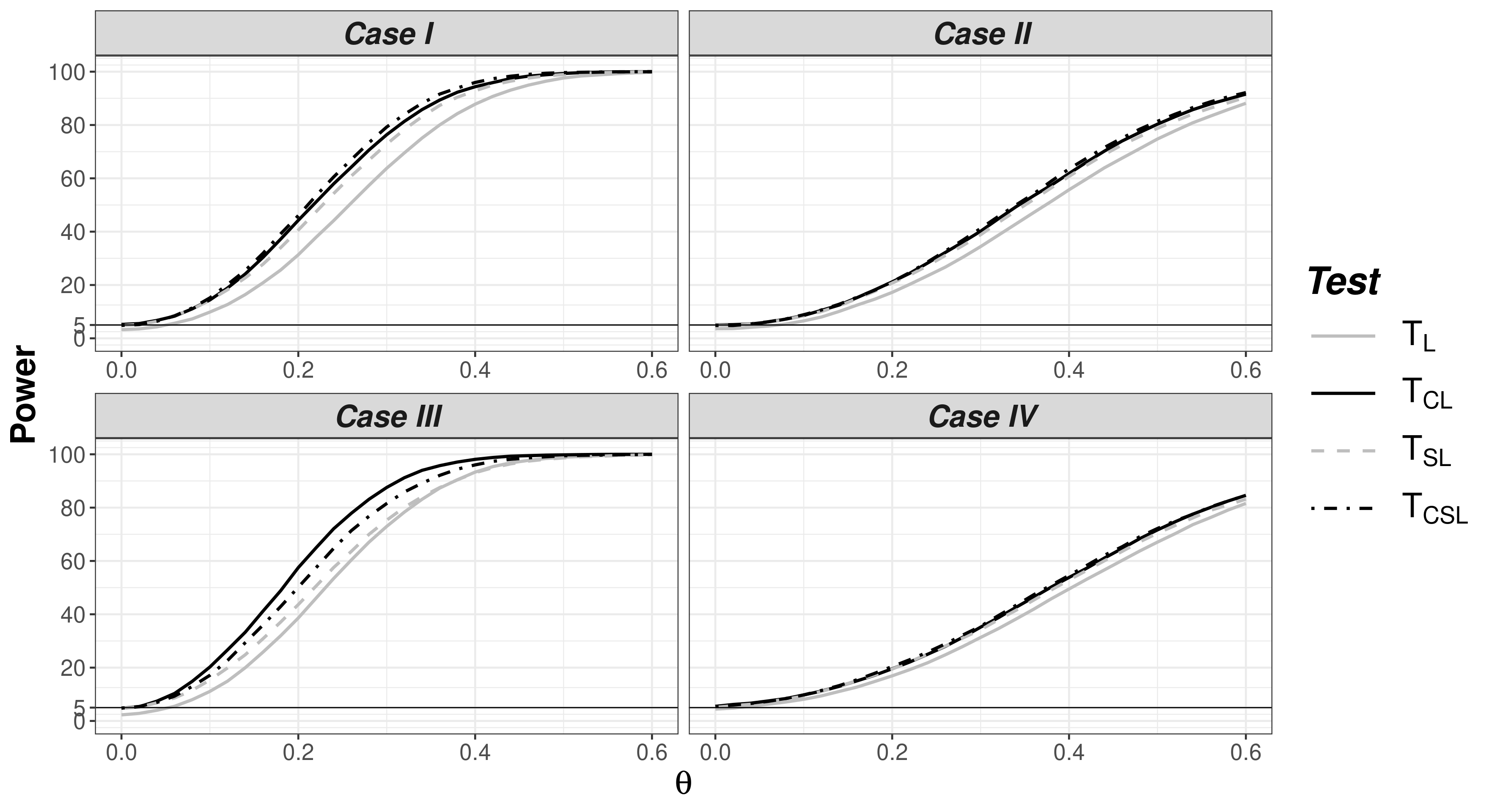
Figure 1: Power curves based on 10,000 simulations

Table 1: Type I errors (in %) based on 10,000 simulations

Case	Randomization		${\cal T}_{\mathrm{L}}$	${\cal T}_{\mathrm{CL}}$	${\cal T}_{\mathrm{SL}}$	${\cal T}_{\mathrm{CSL}}$
I	simple		4.91	5.16	4.86	4.78
	permuted block		3.25	5.22	4.80	4.85
	minimization		3.40	5.43	5.02	5.23
II	simple		5.39	5.14	5.00	4.97
	permuted block		3.59	5.03	4.94	4.82
	minimization		4.01	5.23	5.11	5.28
III	simple		5.07	5.43	5.27	5.16
	permuted block		2.29	4.79	4.76	4.82
	minimization		2.88	5.43	5.23	5.52
IV	simple		5.41	5.30	5.39	5.21
	permuted block		4.44	5.48	5.10	5.49
	minimization		4.21	5.18	5.04	5.06

Table 2: Statistics for the ACTG 175 example

			Sub-group
	All patients		$Z=1$	$Z=2$	$Z=3$
Number of patients	1,093		461	198	434
Log-rank
$\sqrt{n}\widehat{U}_{\mathrm{L}}$	-1.223		-0.542	-0.144	-1.292
$\widehat{\sigma}_{\mathrm{L}}$	0.265		0.235	0.270	0.290
p-value (adjusted for sub-group analysis)	<0.001		0.064	1	<0.001
Estimated $\theta$	-0.528		-0.455	-0.140	-0.740
Standard error of the estimated $\theta$	0.116		0.199	0.263	0.171
Covariate-adjusted log-rank
$\sqrt{n}\widehat{U}_{\mathrm{CL}}$	-1.273		-0.553	-0.129	-1.382
$\widehat{\sigma}_{\mathrm{CL}}$	0.257		0.230	0.265	0.282
p-value (adjusted for sub-group analysis)	<0.001		0.049	1	<0.001
Estimated $\theta$	-0.550		-0.464	-0.127	-0.793
Standard error of the estimated $\theta$	0.113		0.195	0.257	0.166
Stratified log-rank
$\sqrt{n}\widehat{U}_{\mathrm{SL}}$	-1.228
$\widehat{\sigma}_{\mathrm{SL}}$	0.264
p-value	<0.001
Estimated $\theta$	-0.531
Standard error of the estimated $\theta$	0.116
Covariate-adjusted stratified log-rank
$\sqrt{n}\widehat{U}_{\mathrm{CSL}}$	-1.284
$\widehat{\sigma}_{\mathrm{CSL}}$	0.258
p-value	<0.001
Estimated $\theta$	-0.556
Standard error of the estimated $\theta$	0.113
$\theta$ respectively denotes log hazard ratio for all patients and for each subgroup.

Supplementary Materials

1 Additional Simulations

1.1 Additional simulations with $n=500$ under Case I-IV

Based on 10,000 simulations, power curves of four tests for $\theta$ ranging from 0 to 0.6 under simple randomization and minimization are in Figure S1.

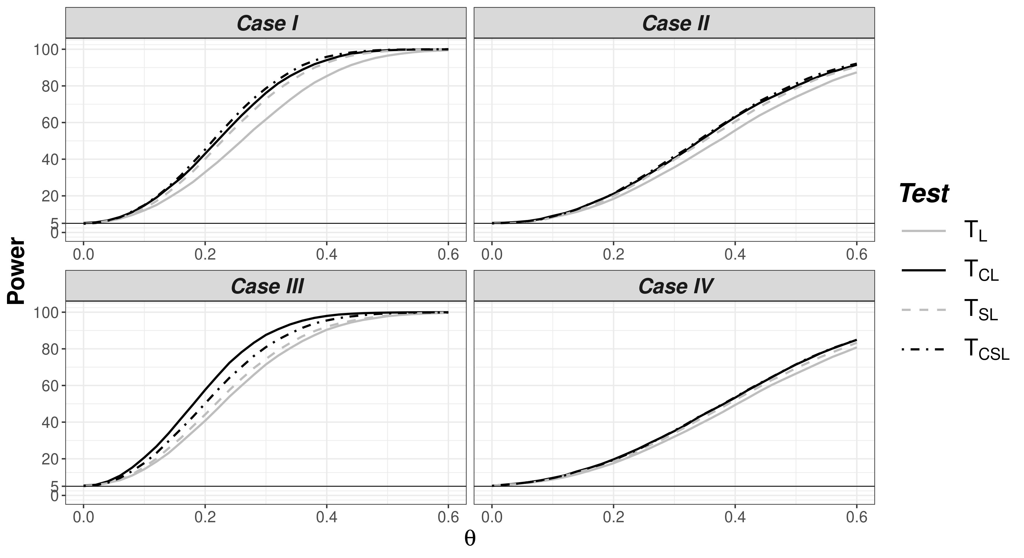
Figure S1: Power curves based on 10,000 simulations with $n=500$ under simple randomization (top) and minimization (bottom).

1.2 Simulations with $n=200$ under Case I-IV

The simulation setting is the same as the simulations in the main article, except that $n=200$ and $Z$ is the 2-dimensional vector whose first component is a two-level discretized first component of $W$ and second component is a two-level discretized second component of $W$. Thus, the average sample size in each treatment and $Z$-level combination is $200/(2\times 4)=25$. Type I error rates for four tests under four cases and three randomization schemes are shown in Table S1. Power curves under three randomization schemes are in Figure S2. From Table S1, we see that with a smaller sample size, the type I error rates of the two covariate-adjusted tests $\mathcal{T}_{\mathrm{CL}}$ and $\mathcal{T}_{\mathrm{CSL}}$ can be slightly inflated but the inflation is not too severe. Otherwise, the results with $n=200$ are similar to the results with $n=500$.

Table S1: Type I errors (in %) based on 10,000 simulations with $n=200$

Case	Randomization	${\cal T}_{\mathrm{L}}$	$\mathcal{T}_{\mathrm{CL}}$	${\cal T}_{\mathrm{SL}}$	${\cal T}_{\mathrm{CSL}}$
Case I	simple	4.90	5.34	4.94	5.01
	permuted block	3.29	5.00	5.07	4.92
	minimization	3.36	5.03	5.01	5.24
Case II	simple	5.05	5.59	5.16	5.28
	permuted block	4.19	5.37	4.86	4.92
	minimization	4.04	5.42	4.92	5.27
Case III	simple	4.88	5.53	5.12	5.18
	permuted block	2.98	5.44	5.28	5.32
	minimization	3.28	5.60	5.46	5.52
Case IV	simple	4.85	5.36	5.19	5.39
	permuted block	4.16	5.19	4.87	4.96
	minimization	4.64	5.64	5.35	5.38

Figure S2: Power curves based on 10,000 simulations with $n=200$ under permuted block randomization (previous page), simple randomization (top this page), and minimization (bottom this page).

1.3 Simulations under violations of Assumption CR

This simulation setting is the same as Case III, except that $C_{j}$ follows a Cox model with conditional hazard $\log(1.1)\exp(-\psi j+\eta_{C}^{\top}W)$ for $j=0,1$, $\psi$ ranges from 0 to 1 for different extent of assumption violation, and $\eta_{C}=(0.2,0.2,0.2)^{\top}$. Type I error rates for four tests under three randomization schemes are shown in Table S2. It can be seen that type I error is inflated as $\psi$ becomes larger.

Table S2: Type I errors (in %) based on 10,000 simulations with $n=500$ when Assumption CR is violated.

Randomization	$\psi$	${\cal T}_{\mathrm{L}}$	${\cal T}_{\mathrm{CL}}$	${\cal T}_{\mathrm{SL}}$	${\cal T}_{\mathrm{CSL}}$
simple	0.0	4.89	5.14	5.12	4.80
	0.1	4.84	5.21	5.22	4.93
	0.2	5.00	5.23	5.15	5.12
	0.3	5.27	5.59	5.29	5.03
	0.4	5.35	5.96	5.41	5.30
	0.5	5.84	6.51	5.34	5.40
	0.6	6.34	7.25	5.35	5.75
	0.7	6.79	7.99	5.76	5.82
	0.8	7.85	8.95	5.94	5.93
	0.9	8.63	10.07	6.12	6.43
	1.0	9.70	11.60	6.52	6.94
permuted block	0.0	3.41	5.36	5.40	4.86
	0.1	3.38	5.49	5.43	5.04
	0.2	3.37	5.36	5.36	4.97
	0.3	3.63	5.79	5.41	5.20
	0.4	3.87	6.04	5.44	5.20
	0.5	4.27	6.76	5.60	5.30
	0.6	4.62	7.08	5.69	5.43
	0.7	5.28	7.68	5.84	5.68
	0.8	5.78	8.84	6.06	5.95
	0.9	6.53	9.90	6.35	6.39
	1.0	7.52	11.34	6.71	6.81
minimization	0.0	3.13	5.26	5.15	5.10
	0.1	3.11	5.27	5.10	5.08
	0.2	3.28	5.54	5.26	5.14
	0.3	3.42	5.72	5.18	4.97
	0.4	3.63	6.19	5.08	5.10
	0.5	4.10	6.87	5.17	5.27
	0.6	4.45	7.46	5.55	5.38
	0.7	5.14	8.10	5.55	5.65
	0.8	5.74	9.02	5.69	6.06
	0.9	6.48	10.15	5.92	6.25
	1.0	7.39	11.15	6.50	6.57

2 Lemmas and Additional theoretical results

2.1 Asymptotic optimality

Consider a general class of log-rank score functions

$$\widehat{U}_{\mathrm{CL}}(b_{0},b_{1}) =\frac{1}{n}\sum_{i=1}^{n}\left[I_{i}\{{O}_{i1}-(X_{i}-\bar{X})^{\top}b_{1}\}-(1-I_{i})\{{O}_{i0}-(X_{i}-\bar{X})^{\top}b_{0}\}\right]+n^{-1/2}o_{p}(1),$$

where $b_{1}$ and $b_{0}$ are any fixed constants. The following theorem derives the asymptotic distribution of $\widehat{U}_{\mathrm{CL}}(b_{0},b_{1})$, and shows that $\widehat{U}_{\mathrm{CL}}(\beta_{0},\beta_{1})$ has the smallest variance.

Theorem S1.

Assume (D), (D^†), and that all levels of $Z$ used in covariate-adaptive randomization are included in $X_{i}$ as a sub-vector. Then the following results hold.

$$\sqrt{n}\left(\widehat{U}_{\mathrm{CL}}(b_{0},b_{1})-\frac{n_{1}\theta_{1}-n_{0}\theta_{0}}{n}\right)\xrightarrow{d}N\left(0,\sigma_{\mathrm{CL}}^{2}(b_{0},b_{1})\right),$$

where

$$\sigma_{\mathrm{CL}}^{2}(b_{0},b_{1})= \pi E\left\{{\rm var}({O}_{i1}-X_{i}^{\top}b_{1}\mid Z_{i})\right\}+(1-\pi)E\left\{{\rm var}({O}_{i0}-X_{i}^{\top}b_{0}\mid Z_{i})\right\}$$

$$\qquad+\nu{\rm var}\left\{E({O}_{i1}-X_{i}^{\top}b_{1}\mid Z_{i})+E({O}_{i0}-X_{i}^{\top}b_{0}\mid Z_{i})\right\}$$

$$\qquad+{\rm var}\left\{\pi E({O}_{i1}-X_{i}^{\top}b_{1}\mid Z_{i})-(1-\pi)E({O}_{i0}-X_{i}^{\top}b_{0}\mid Z_{i})\right\}$$

$$\qquad+\{2\pi\beta_{1}-2(1-\pi)\beta_{0}-\pi b_{1}+(1-\pi)b_{0}\}^{\top}{\rm var}(X_{i})\{\pi b_{1}-(1-\pi)b_{0}\}.$$

Furthermore,

$$\sigma^{2}_{\mathrm{CL}}(b_{0},b_{1})-\sigma^{2}_{\mathrm{CL}}(\beta_{0},\beta_{1})$$

$$=\pi(1-\pi)(\beta_{1}-b_{1}+\beta_{0}-b_{0})^{\top}\left[E\{{\rm var}(X_{i}\mid Z_{i})\}+\frac{\nu}{\pi(1-\pi)}{\rm var}\{E(X_{i}\mid Z_{i})\}\right](\beta_{1}-b_{1}+\beta_{0}-b_{0})$$

which is $\geq 0$ with strict inequality holding unless $\beta_{1}+\beta_{0}=b_{0}+b_{1}$ or ${\rm var}(X_{i}\mid Z_{i})=0$ and $\nu=0$ almost surely.

To end this section we emphasize that the use of $\widehat{O}_{ij}$’s in (3) as derived outcomes to reduce variability of $\widehat{U}_{\mathrm{L}}$ is a key to our results. The use of other derived outcomes may not achieve guaranteed efficiency gain. For example, Tangen and Koch, (1999) and Jiang et al., (2008) considered log-rank scores $\widetilde{O}_{ij}=\int_{0}^{\tau}{\textstyle\frac{1}{2}}\big{\{}dN_{ij}(t)-Y_{ij}(t)d\bar{N}(t)/\bar{Y}(t)\big{\}}$ as derived outcomes; however, using $\widetilde{O}_{ij}$ to replace $\widehat{O}_{ij}$ in (4) and (5) produces an adjusted score that is not necessarily more efficient than the unadjusted $\widehat{U}_{\mathrm{L}}$ and is always less efficient than $\widehat{U}_{\mathrm{CL}}$ in (4) (as shown in Theorem S1), due to the reason that using $\widetilde{O}_{ij}$ instead of $\widehat{O}_{ij}$ in (5) does not correctly capture the true correlation between ${O}_{ij}$ and $X_{i}$. Furthermore, using $\widetilde{O}_{ij}$ may not produce a valid test under covariate-adaptive randomization, even with (C)-(D) and all joint levels of $Z_{i}$ included in $X_{i}$.

2.2 Covariate adjustment in hazard ratio estimation under Cox model

After testing the null hypothesis of no treatment effect using the covariate-adjusted log-rank test $\mathcal{T}_{\mathrm{CL}}$, it is of interest to also report an effect size estimate and confidence interval. One common parameter is the hazard ratio $e^{\theta}$ under the Cox proportional hazards model

$$\lambda_{1}(t)=\lambda_{0}(t)e^{\theta}.$$

Without using covariates, the score equation from the partial likelihood is

$$\widehat{U}_{\mathrm{L}}(\vartheta)=\frac{1}{n}\sum_{i=1}^{n}\int_{0}^{\tau}\left\{I_{i}-\frac{S^{(1)}(\vartheta,t)}{S^{(0)}(\vartheta,t)}\right\}dN_{i}(t),$$

where $S^{(1)}(\vartheta,t)=n^{-1}\sum_{i=1}^{n}I_{i}Y_{i}(t)e^{\vartheta I_{i}}=e^{\vartheta}\bar{Y}_{1}(t)$ and $S^{(0)}(\vartheta,t)=n^{-1}\sum_{i=1}^{n}Y_{i}(t)e^{\vartheta I_{i}}=e^{\vartheta}\bar{Y}_{1}(t)+\bar{Y}_{0}(t)$. The log-rank test uses $\widehat{U}_{\mathrm{L}}(0)$.

Let

$$O_{i1}(\theta) =\int_{0}^{\tau}\left\{1-\frac{s^{(1)}(\theta,t)}{s^{(0)}(\theta,t)}\right\}\left\{dN_{i1}(t)-Y_{i1}(t)e^{\theta}\frac{E(dN_{i}(t))}{s^{(0)}(\theta,t)}\right\}$$

$$O_{i0}(\theta) =\int_{0}^{\tau}\frac{s^{(1)}(\theta,t)}{s^{(0)}(\theta,t)}\left\{dN_{i0}(t)-Y_{i0}(t)\frac{E(dN_{i}(t))}{s^{(0)}(\theta,t)}\right\},$$

where $s^{(1)}(\theta,t)=e^{\theta}\mu(t)E\{Y_{i}(t)\}$ and $s^{(0)}(\theta,t)=\{e^{\theta}\mu(t)+1-\mu(t)\}E\{Y_{i}(t)\}$.

Theorem S2.

Assume (C) and (D), and all joint levels of $Z_{i}$ used in covariate-adaptive randomization are included in $X_{i}$ as a sub-vector. Also assume the Cox proportional hazards model $\lambda_{1}(t)=\lambda_{0}(t)e^{\theta}$. Then, the following results hold regardless of which covariate-adaptive randomization scheme is applied.

$$\sqrt{n}(\widehat{\theta}_{\mathrm{CL}}-\theta)\xrightarrow{d}N\left(0,\frac{\sigma_{\mathrm{CL}}^{2}(\theta)}{\sigma^{4}_{\mathrm{L}}(\theta)}\right),$$

where $\sigma_{\mathrm{CL}}^{2}(\theta)=\sigma_{\mathrm{L}}^{2}(\theta)-\pi(1-\pi)(\beta_{1}(\theta)+\beta_{0}(\theta))^{\top}\Sigma_{X}(\beta_{1}(\theta)+\beta_{0}(\theta))$,

$$\sigma_{\mathrm{CL}}^{2}(\theta) =\pi\mathrm{var}(O_{i1}(\theta)-X_{i}^{\top}\beta_{1}(\theta))+(1-\pi)\mathrm{var}(O_{i0}(\theta)-X_{i}^{\top}\beta_{0}(\theta))$$

$$\quad+(\pi\beta_{1}(\theta)-(1-\pi)\beta_{0}(\theta))^{\top}\Sigma_{X}(\pi\beta_{1}(\theta)-(1-\pi)\beta_{0}(\theta)),$$

$$\sigma_{\mathrm{L}}^{2}(\theta) =\pi{\rm var}(O_{i1}(\theta))+(1-\pi){\rm var}(O_{i0}(\theta)),$$

and $\beta_{j}(\theta)=\Sigma_{X}^{-1}\mathrm{cov}(X_{i},O_{ij}(\theta))$ for $j=0,1$.

Inference can be made based on Theorem S2 and estimated variance $\widehat{\sigma}^{2}_{\mathrm{CL}}(\widehat{\theta}_{\mathrm{CL}})/\widehat{\sigma}^{4}_{\mathrm{L}}(\widehat{\theta}_{\mathrm{CL}})$, with

$$\widehat{\sigma}^{2}_{\mathrm{L}}(\widehat{\theta}_{\mathrm{CL}})=-\partial\widehat{U}_{\mathrm{L}}(\vartheta)/\partial\vartheta\mid_{\vartheta=\widehat{\theta}_{\mathrm{CL}}}=n^{-1}\sum_{i=1}^{n}\int_{0}^{\tau}\frac{e^{\widehat{\theta}_{\mathrm{CL}}}\bar{Y}_{1}(t)\bar{Y}_{0}(t)}{\{e^{\widehat{\theta}_{\mathrm{CL}}}\bar{Y}_{1}(t)+\bar{Y}_{0}(t)\}^{2}}dN_{i}(t)$$

and $\widehat{\sigma}^{2}_{\mathrm{CL}}(\widehat{\theta}_{\mathrm{CL}})=\widehat{\sigma}^{2}_{\mathrm{L}}(\widehat{\theta}_{\mathrm{CL}})-\pi(1-\pi)(\widehat{\beta}_{1}(\widehat{\theta}_{\mathrm{L}}))+\widehat{\beta}_{0}(\widehat{\theta}_{\mathrm{L}}))^{\top}\widehat{\Sigma}_{X}(\widehat{\beta}_{1}(\widehat{\theta}_{\mathrm{L}}))+\widehat{\beta}_{0}(\widehat{\theta}_{\mathrm{L}}))$.

2.3 Covariate adjustment in hazard ratio estimation under stratified Cox model

In this section, we assume the stratified Cox proportional hazards model:

$$\lambda_{z1}(t)=\lambda_{z0}(t)e^{\theta}.$$

Without using covariates, the score equation from the partial likelihood is

$$\widehat{U}_{\mathrm{SL}}(\vartheta)=n^{-1}\sum_{z}\sum_{i\mathrel{\mathop{\ordinarycolon}}Z_{i}=z}\int_{0}^{\tau}\bigg{\{}I_{i}-\frac{S_{z}^{(1)}(\vartheta,t)}{S_{z}^{(0)}(\vartheta,t)}\bigg{\}}dN_{i}(t).$$

where $S_{z}^{(1)}(\vartheta,t)=n^{-1}\sum_{i\mathrel{\mathop{\ordinarycolon}}Z_{i}=z}I_{i}Y_{i}(t)e^{\vartheta I_{i}}=e^{\vartheta}\bar{Y}_{z1}(t)$ and $S_{z}^{(0)}(\vartheta,t)=n^{-1}\sum_{i\mathrel{\mathop{\ordinarycolon}}Z_{i}=z}Y_{i}(t)e^{\vartheta I_{i}}=e^{\vartheta}\bar{Y}_{z1}(t)+\bar{Y}_{z0}(t)$. The log-rank test uses $\widehat{U}_{\mathrm{SL}}(0)$. The maximum partial likelihood estimator $\widehat{\theta}_{\mathrm{SL}}$ of $\theta$ is a solution to $\widehat{U}_{\mathrm{SL}}(\vartheta)=0$. Our covariate-adjusted score is

$$\widehat{U}_{\mathrm{CSL}}(\vartheta) =\widehat{U}_{\mathrm{SL}}(\vartheta)-\frac{1}{n}\sum_{z}\sum_{i\mathrel{\mathop{\ordinarycolon}}Z_{i}=z}\left\{I_{i}(X_{i}-\bar{X}_{z})^{\top}\widehat{\gamma}_{1}(\widehat{\theta}_{\mathrm{SL}})-(1-I_{i})(X_{i}-\bar{X}_{z})^{\top}\widehat{\gamma}_{0}(\widehat{\theta}_{\mathrm{SL}})\right\},$$

where, for $j=0,1$, $\widehat{\gamma}_{j}(\widehat{\theta}_{\mathrm{SL}})$ is equal to $\widehat{\gamma}_{j}$ in the main article with $\widehat{O}_{zij}$ replaced by

$$\widehat{O}_{zij}(\widehat{\theta}_{\mathrm{SL}})=\int_{0}^{\tau}\frac{\{e^{\widehat{\theta}_{\mathrm{SL}}}\bar{Y}_{z1}(t)\}^{(1-j)}\{\bar{Y}_{z0}(t)\}^{j}}{e^{\widehat{\theta}_{\mathrm{SL}}}\bar{Y}_{z1}(t)+\bar{Y}_{z0}(t)}\left\{dN_{ij}(t)-\frac{Y_{ij}(t)e^{j\widehat{\theta}_{\mathrm{SL}}}d\bar{N}_{z}(t)}{e^{\widehat{\theta}_{\mathrm{SL}}}\bar{Y}_{z1}(t)+\bar{Y}_{z0}(t)}\right\}.$$

We obtain $\widehat{\theta}_{\mathrm{CSL}}$ from solving $\widehat{U}_{\mathrm{CSL}}(\vartheta)=0$.

Let

$$O_{zi1}(\theta) =\int_{0}^{\tau}\left\{1-\frac{s_{z}^{(1)}(\theta,t)}{s_{z}^{(0)}(\theta,t)}\right\}\left\{dN_{i1}(t)-Y_{i1}(t)e^{\theta}\frac{E(dN_{i}(t)\mid Z_{i}=z)}{s_{z}^{(0)}(\theta,t)}\right\}$$

$$O_{zi0}(\theta) =\int_{0}^{\tau}\frac{s_{z}^{(1)}(\theta,t)}{s_{z}^{(0)}(\theta,t)}\left\{dN_{i0}(t)-Y_{i0}(t)\frac{E(dN_{i}(t)\mid Z_{i}=z)}{s_{z}^{(0)}(\theta,t)}\right\},$$

where $s_{z}^{(1)}(\theta,t)=e^{\theta}\mu_{z}(t)E\{Y_{i}(t)\}$ and $s_{z}^{(0)}(\theta,t)=\{e^{\theta}\mu_{z}(t)+1-\mu_{z}(t)\}E\{Y_{i}(t)\}$.

Theorem S3.

Under (C-z) and (D). Also assume the Cox proportional hazards model $\lambda_{z1}(t)=\lambda_{z0}(t)e^{\theta}$. Then, the following results hold regardless of which covariate-adaptive randomization scheme is applied.

$$\sqrt{n}(\widehat{\theta}_{\mathrm{CSL}}-\theta)\xrightarrow{d}N\left(0,\frac{\sigma_{\mathrm{CSL}}^{2}(\theta)}{\sigma^{4}_{\mathrm{SL}}(\theta)}\right),$$

where $\sigma_{\mathrm{CSL}}^{2}(\theta)=\sigma_{\mathrm{SL}}^{2}(\theta)-\pi(1-\pi)(\gamma_{1}(\theta)+\gamma_{0}(\theta))^{\top}E\{{\rm var}(X_{i}\mid Z_{i})\}(\gamma_{1}(\theta)+\gamma_{0}(\theta))$, $\sigma_{\mathrm{SL}}^{2}(\theta)=\sum_{z}\mathrm{pr}(Z_{i}=z)\{\pi{\rm var}(O_{zi1}(\theta)\mid Z_{i}=z)+(1-\pi){\rm var}(O_{zi0}(\theta)\mid Z_{i}=z)\}$.

The proof of Theorem S3 is similar to the proof of Theorem S2 and thus is omitted. Based on Theorem S3, inference can be made based on the estimated variance $\widehat{\sigma}^{2}_{\mathrm{CSL}}(\widehat{\theta}_{\mathrm{CSL}})/\widehat{\sigma}^{4}_{\mathrm{SL}}(\widehat{\theta}_{\mathrm{CSL}})$, with

$$\widehat{\sigma}^{2}_{\mathrm{SL}}(\widehat{\theta}_{\mathrm{CSL}}) =-\partial\widehat{U}_{\mathrm{SL}}(\vartheta)/\partial\vartheta\mid_{\vartheta=\widehat{\theta}_{\mathrm{CSL}}}=n^{-1}\sum_{z}\sum_{i\mathrel{\mathop{\ordinarycolon}}Z_{i}=z}\int_{0}^{\tau}\frac{e^{\widehat{\theta}_{\mathrm{CSL}}}\bar{Y}_{z1}(t)\bar{Y}_{z0}(t)}{\{e^{\widehat{\theta}_{\mathrm{CSL}}}\bar{Y}_{z1}(t)+\bar{Y}_{z0}(t)\}^{2}}dN_{i}(t)$$

and $\widehat{\sigma}^{2}_{\mathrm{CSL}}(\widehat{\theta}_{\mathrm{CSL}})=\widehat{\sigma}^{2}_{\mathrm{SL}}(\widehat{\theta}_{\mathrm{CSL}})-\pi(1-\pi)(\widehat{\gamma}_{1}(\widehat{\theta}_{\mathrm{SL}})+\widehat{\gamma}_{0}(\widehat{\theta}_{\mathrm{SL}}))^{\top}\{\sum_{z}(n_{z}/n)\widehat{\Sigma}_{X\mid z}\}(\widehat{\gamma}_{1}(\widehat{\theta}_{\mathrm{SL}})+\widehat{\gamma}_{0}(\widehat{\theta}_{\mathrm{SL}}))$.

2.4 Lemmas

The following lemmas are useful for proving the main theorems.

Lemma S1.

Under condition (D),
(a) $\widehat{\beta}_{1}=\beta_{1}+o_{p}(1)$ and $\widehat{\beta}_{0}=\beta_{0}+o_{p}(1)$.
(b) $\widehat{\gamma}_{1}=\gamma_{1}+o_{p}(1)$ and $\widehat{\gamma}_{0}=\gamma_{0}+o_{p}(1)$.

Lemma S2.

Assume (CR) and (D). Let $E_{H_{0}^{\dagger}}$, $\lambda_{H_{0}^{\dagger}}$, $\mu_{H_{0}^{\dagger}}(t)$, and $p_{H_{0}^{\dagger}}(t)$ be the expectation, hazard, $\mu(t)$, and $p(t)$ under the null hypothesis $H_{0}^{\dagger}\mathrel{\mathop{\ordinarycolon}}\lambda_{1}(t,v)=\lambda_{0}(t,v)$ for all $t$ and $v$, where $\lambda_{j}(t,v)$ is the true hazard function of $T_{j}$ conditional on $V=v$ for $j=0,1$, and $V$ is in (CR). Then, for any $t$,
(a) $E_{H_{0}^{\dagger}}\{I_{i}Y_{i}(t)\mid V_{i}\}=\pi E_{H_{0}^{\dagger}}\{Y_{i1}(t)\mid V_{i}\}=\mu_{H_{0}^{\dagger}}(t)E_{H_{0}^{\dagger}}\{Y_{i}(t)\mid V_{i}\},$
(b) $E_{H_{0}^{\dagger}}\{(1-I_{i})Y_{i}(t)\mid V_{i}\}=(1-\pi)E_{H_{0}^{\dagger}}\{Y_{i0}(t)\mid V_{i}\}=\{1-\mu_{H_{0}^{\dagger}}(t)\}E_{H_{0}^{\dagger}}\{Y_{i}(t)\mid V_{i}\},$
(c) $E_{H_{0}^{\dagger}}\{Y_{ij}(t)\lambda_{H_{0}^{\dagger}}(t,V_{i})\}=p_{H_{0}^{\dagger}}(t)E_{H_{0}^{\dagger}}\{Y_{ij}(t)\},\ j=0,1.$

Note that conditions (C) and (D) imply Lemma S2 to hold with $V=\emptyset$. In addition, as (TR) leads to the equivalence of $H_{0}$ and $H_{0}^{\dagger}$, thus, (CR), (TR) and (D) imply Lemmas S2(a)-(c) to also hold under $H_{0}$.

Lemma S3.

Let $\widetilde{\sigma}_{\mathrm{L}}^{2}=\int_{0}^{\tau}\mu(t)\{1-\mu(t)\}E\{dN_{i}(t)\}$. Assume (CR) and (D), $\widehat{\sigma}_{\mathrm{L}}^{2}\xrightarrow{p}\widetilde{\sigma}_{\mathrm{L}}^{2}$ and

$$\widetilde{\sigma}_{\mathrm{L}}^{2}=\int_{0}^{\tau}E\left[\mu(t)\{1-\mu(t)\}\{\pi Y_{i1}(t)\lambda_{1}(t,V_{i})+(1-\pi)Y_{i0}(t)\lambda_{0}(t,V_{i})\}\right]dt.$$

Lemma S4.

Assume the conditions in Theorem 1 and the local alternative hypothesis specified in Theorem 1(c). Then, $E(O_{ij})\to 0$, $j=0,1$, and both $\sigma^{2}_{\mathrm{L}}$ and $\widetilde{\sigma}_{\mathrm{L}}^{2}\to\pi{\rm var}_{H_{0}}(O_{i1})+(1-\pi){\rm var}_{H_{0}}(O_{i0})$, where ${\rm var}_{H_{0}}$ denotes the variance under $H_{0}$.

3 Technical Proofs

3.1 Proofs of Lemmas

Proof of Lemma S1.
(a) We show the proof for $\widehat{\beta}_{1}$ and $\beta_{1}$. Note first that

$$\frac{1}{n_{1}}\sum_{i=1}^{n}I_{i}(X_{i}-\bar{X}_{1})(X_{i}-\bar{X}_{1})^{\top}\xrightarrow{p}\Sigma_{X}$$

from the proof of Lemma 3 in Ye et al., (2022). From Lemma 3 of Ye and Shao, (2020), we have that $\bar{Y}_{0}(t)\xrightarrow{p}(1-\pi)E\{Y_{i0}(t)\},\bar{Y}_{1}(t)\xrightarrow{p}\pi E\{Y_{i1}(t)\},\bar{Y}(t)\xrightarrow{p}E\{Y_{i}(t)\}$. Similarly, we can show that $n_{1}^{-1}\sum_{i=1}^{n}I_{i}X_{i}dN_{i1}(t)\xrightarrow{p}E\{X_{i}dN_{i1}(t)\}$, $n_{1}^{-1}\sum_{i=1}^{n}I_{i}X_{i}Y_{i1}(t)\xrightarrow{p}E\{X_{i}Y_{i1}(t)\}$, and $\bar{N}(t)\xrightarrow{p}E\{N_{i}(t)\}$. Hence,

$$\frac{1}{n_{1}}\sum_{i=1}^{n}I_{i}(X_{i}-\bar{X}_{1})\widehat{O}_{i1}\xrightarrow{p}{\rm cov}(X_{i},{O}_{i1}),$$

concluding the proof that $\widehat{\beta}_{1}=\beta_{1}+o_{p}(1)$. The result for $\widehat{\beta}_{0}$ can be shown in the same way.
(b) The proof for $\widehat{\gamma}_{1},\widehat{\gamma}_{0}$ and $\gamma_{1},\gamma_{0}$ are similar and can be established from showing

$$\frac{1}{n_{1}}\sum_{z}\sum_{i\mathrel{\mathop{\ordinarycolon}}Z_{i}=z}I_{i}(X_{i}-\bar{X}_{z1})(X_{i}-\bar{X}_{z1})^{\top} \xrightarrow{p}E\{{\rm var}(X_{i}\mid Z_{i})\}$$

$$\frac{1}{n_{1}}\sum_{z}\sum_{i\mathrel{\mathop{\ordinarycolon}}Z_{i}=z}I_{i}(X_{i}-\bar{X}_{z1})\widehat{O}_{zi1} \xrightarrow{p}\sum_{z}P(Z=z){\rm cov}\left(X_{i},O_{zi1}\mid Z_{i}=z\right)$$

$$={\rm cov}\left(X_{i},\sum_{z}I(Z_{i}=z)(O_{zi1}-\theta_{z1})\right),$$

where $\gamma_{j}=E\{{\rm var}(X_{i}\mid Z_{i})\}^{-1}{\rm cov}\left(X_{i},\sum_{z}I(Z_{i}=z)(O_{zij}-\theta_{zj})\right)$.

Proof of Lemma S2.
For simplicity, we remove the subscript $H_{0}^{\dagger}$ and assume all calculations are under $H_{0}^{\dagger}$.
(a) Note that

$$\pi E\{Y_{i1}(t)\mid V_{i}\}=E\left[E(I_{i}\mid Z_{1},\dots,Z_{n},V_{i})E\{Y_{i1}(t)\mid Z_{1},\dots,Z_{n},V_{i}\}\mid V_{i}\right]$$

$$=E\left[I_{i}Y_{i}(t)\mid V_{i}\right]=E\left[E\{I_{i}\mid Y_{i}(t)=1,V_{i}\}Y_{i}(t)\mid V_{i}\right]$$

$$=\mu(t)E\left\{Y_{i}(t)\mid V_{i}\right\},$$

where the first equality is because of $E(I_{i}\mid Z_{1},\dots,Z_{n},V_{i})=E(I_{i}\mid Z_{1},\dots,Z_{n})=\pi$, the second equality is because of the conditional independence $I_{i}\perp Y_{i1}(t)\mid Z_{1},\dots,Z_{n},V_{i}$ implied by (D), the last equality is from $E\{I_{i}\mid Y_{i}(t)=1,V_{i}\}=\mu(t)$ under (CR) and $H_{0}^{\dagger}$ due to Lemma 1 in Ye and Shao, (2020).
(b) The proof is the same as that for (a).
(c) The result is straightforward from showing that

$$E\{Y_{i1}(t)\lambda(t,V_{i})\} =\pi^{-1}E\{I_{i}Y_{i}(t)\lambda(t,V_{i})\}=\pi^{-1}E\left[E\{I_{i}\mid Y_{i}(t)=1,V_{i}\}Y_{i}(t)\lambda(t,V_{i})\right]$$

$$=\pi^{-1}\mu(t)E\left[Y_{i}(t)\lambda(t,V_{i})\right]=\pi^{-1}\mu(t)E\left[Y_{i}(t)\right]p(t)$$

$$E\{Y_{i1}(t)\} =\pi^{-1}E\{I_{i}Y_{i}(t)\}=\pi^{-1}E\left[E\{I_{i}\mid Y_{i}(t)=1\}Y_{i}(t)\right]$$

$$=\pi^{-1}\mu(t)E\left[Y_{i}(t)\right],$$

as well as the counterparts for $E\{Y_{i0}(t)\lambda(t,V_{i})\}$ and $E\{Y_{i0}(t)\}$.

Proof of Lemma S3.
The first result $\widehat{\sigma}_{\mathrm{L}}^{2}\xrightarrow{p}\widetilde{\sigma}_{\mathrm{L}}^{2}$ is because $\bar{Y}_{1}(t)\bar{Y}_{0}(t)/\bar{Y}(t)^{2}\xrightarrow{p}\mu(t)\{1-\mu(t)\}$ from Lemma 3 of Ye and Shao, (2020), and $d\bar{N}(t)\xrightarrow{p}E\{dN_{i}(t)\}$.

Then, under (CR), from the theory of counting processes in survival analysis (Andersen and Gill,, 1982), the process $N_{ij}(t)$ has random intensity process of the form $Y_{ij}(t)\lambda_{j}(t,V_{i})$, $j=0,1$. Hence, for $i=1,...,n$, $j=0,1,$ the process $N_{ij}(t)-\int_{0}^{t}Y_{ij}(s)\lambda_{j}(s,V_{i})ds$ is a local square integrable martingale with respect to the filtration ${\cal F}_{t}=\sigma\{N_{ij}(u),(1-\delta_{ij}){\cal I}(X_{ij}\leq u),V_{i}\mathrel{\mathop{\ordinarycolon}}0\leq u\leq t\}$. From the fact that martingales have expectation zero, we conclude that $E\{dN_{ij}(t)\}=E\{Y_{ij}(t)\lambda_{j}(t,V_{i})\}dt$. The second result follows from

$$E\{dN_{i}(t)\} =E\{I_{i}dN_{i1}(t)+(1-I_{i})dN_{i0}(t)\}$$

$$=\pi E\{Y_{i1}(t)\lambda_{1}(t,V_{i})\}dt+(1-\pi)E\{Y_{i0}(t)\lambda_{0}(t,V_{i})\}dt.$$

Proof of Lemma S4.
Let $V_{i}=\emptyset$ under (C), and $V_{i}$ is the $V_{i}$ in (CR) under (CR)-(TR). Then,

$$E(O_{i1})=\int_{0}^{\tau}E[\{1-\mu(t)\}Y_{i1}(t)\{\lambda_{1}(t,V_{i})-p(t)\}]dt.$$

Under the local alternative and from the dominated convergence theorem, for every $t$,

$$E\{Y_{i1}(t)\} =\int e^{-\int_{0}^{t}\lambda_{1}(s,v)ds}{\rm pr}(C_{1}\geq t\mid V=v)dF(v)$$

$$\rightarrow\int e^{-\int_{0}^{t}\lambda_{H_{0}^{\dagger}}(s,v)ds}{\rm pr}(C_{1}\geq t\mid V=v)dF(v)$$

$$=E_{H_{0}^{\dagger}}\{Y_{i1}(t)\},$$ (S1)

where $F$ is the distribution of $V$ and $\lambda_{H_{0}^{\dagger}}$ and $E_{H_{0}^{\dagger}}$ denote the hazard and expectation under $H_{0}^{\dagger}$ defined in Lemma S2, respectively. Similarly, we can show that

$$E\left\{Y_{i1}(t)\lambda_{1}(t,V_{i})\right\}\rightarrow E_{H_{0}^{\dagger}}\left\{Y_{i1}(t)\lambda_{H_{0}^{\dagger}}(t,V_{i})\right\}.$$ (S2)

These imply that $\mu(t)\rightarrow\mu_{H_{0}^{\dagger}}(t)$ and $p(t)\rightarrow p_{H_{0}^{\dagger}}(t)$, where $\mu_{H_{0}^{\dagger}}(t)$ and $p_{H_{0}^{\dagger}}(t)$ are $\mu(t)$ and $p(t)$ under $H_{0}^{\dagger}$, respectively. Hence, again from the dominant convergence theorem,

$$E(O_{i1}) =\int_{0}^{\tau}\{1-\mu(t)\}E[Y_{i1}(t)\{\lambda_{1}(t,V_{i})-p(t)\}]dt$$

$$\to\int_{0}^{\tau}\{1-\mu_{H_{0}^{\dagger}}(t)\}E_{H_{0}^{\dagger}}[Y_{i1}(t)\{\lambda_{H_{0}^{\dagger}}(t,V_{i})-p_{H_{0}^{\dagger}}(t)\}]dt$$

$$=E_{H_{0}^{\dagger}}(O_{i1})$$

$$=0$$

where the last equality follows from Lemma S2(c). The proof for $E(O_{i0})\to 0$ is the same.

Let ${\rm var}_{H_{0}}$ denote the variance under $H_{0}$. Theorem S1 with $b_{0}=b_{1}=0$ implies that $\sigma_{\mathrm{L}}^{2}=\pi{\rm var}(O_{i1})+(1-\pi){\rm var}(O_{i0})$. Next, we show that under the local alternative, $\sigma_{\mathrm{L}}^{2}\to\pi{\rm var}_{H_{0}^{\dagger}}(O_{i1})+(1-\pi){\rm var}_{H_{0}^{\dagger}}(O_{i0})$. For ${\rm var}(O_{ij})$, since ${\rm var}(O_{ij})=E(O_{ij}^{2})-\{E(O_{ij})\}^{2}$ and $E(O_{ij})\to 0$, it suffices to show that $E(O_{ij}^{2})\to{\rm var}_{H_{0}^{\dagger}}(O_{ij}^{2})$. Note that

$$E(O_{i1}^{2}) =E\left[\bigg{\{}\int_{0}^{\tau}\{1-\mu(t)\}dN_{i1}(t)\bigg{\}}^{2}\right.$$

$$\quad-2\int_{0}^{\tau}\int_{0}^{\tau}\{1-\mu(t)\}Y_{i1}(t)\lambda_{1}(t,V_{i})\{1-\mu(s)\}Y_{i1}(s)p(s)dtds$$

$$\left.\quad+\int_{0}^{\tau}\int_{0}^{\tau}\{1-\mu(t)\}\{1-\mu(s)\}Y_{i1}(s)Y_{i1}(t)p(s)p(t)dtds\right]$$

$$=\int_{0}^{\tau}\{1-\mu(t)\}^{2}E\left\{dN_{i1}(t)\right\}$$

$$\qquad-2\int_{0}^{\tau}\int_{t\geq s}\{1-\mu(t)\}\{1-\mu(s)\}p(s)E\{Y_{i1}(t)\lambda_{1}(t,V_{i})-Y_{i1}(t)p(t)\}dtds,$$

where the second equality is because, when $t>s$, $Y_{i1}(t)dN_{i1}(s)=0$, $E\{Y_{i1}(s)dN_{i1}(t)\mid\mathcal{F}_{t-}\}=Y_{i1}(s)Y_{i1}(t)\lambda_{1}(t,V_{i})dt$ for $t\geq s$, and $Y_{i1}(t)Y_{i1}(s)=Y_{i1}\{\max(t,s)\}$. These techniques will be used frequently in the following proofs, and will not be further elaborated. From (S1)-(S2), we have that $E\{Y_{i1}(t)\lambda_{1}(t,V_{i})-Y_{i1}(t)p(t)\}\to 0$ for every $t$, and consequently

$$E(O_{i1}^{2})\to\int_{0}^{\tau}\{1-\mu_{H_{0}^{\dagger}}(t)\}^{2}E_{H_{0}^{\dagger}}\left\{Y_{i1}(t)\lambda_{H_{0}^{\dagger}}(t,V_{i})\right\}dt,$$

which is equal to ${\rm var}_{H_{0}^{\dagger}}(O_{i1})$ by the same argument and the fact that $E_{H_{0}^{\dagger}}(O_{i1})=0$. Similarly, we can show that $E(O_{i0}^{2})\to\int_{0}^{\tau}\mu_{H_{0}^{\dagger}}(t)^{2}E_{H_{0}^{\dagger}}\left\{Y_{i0}(t)\lambda_{H_{0}^{\dagger}}(t,V_{i})\right\}dt={\rm var}_{H_{0}^{\dagger}}(O_{i0})$. This concludes the proof that $\sigma_{\mathrm{L}}^{2}\to\pi{\rm var}_{H_{0}^{\dagger}}(O_{i1})+(1-\pi){\rm var}_{H_{0}^{\dagger}}(O_{i0})$ under the local alternative.

For $\widetilde{\sigma}_{\mathrm{L}}^{2}$, under the local alternative, from Lemma S2, (S1)-(S2), and a similar argument as above,

$$\widetilde{\sigma}_{\mathrm{L}}^{2} =\int_{0}^{\tau}\mu(t)\{1-\mu(t)\}\left[\pi E\{Y_{i1}(t)\lambda_{1}(t,V_{i})\}+(1-\pi)E\{Y_{i0}(t)\lambda_{0}(t,V_{i})\}\right]dt$$

$$\to\int_{0}^{\tau}\mu_{H_{0}^{\dagger}}(t)\{1-\mu_{H_{0}^{\dagger}}(t)\}\left[\pi E_{H_{0}^{\dagger}}\{Y_{i1}(t)\lambda_{H_{0}^{\dagger}}(t,V_{i})\}+(1-\pi)E_{H_{0}^{\dagger}}\{Y_{i0}(t)\lambda_{H_{0}^{\dagger}}(t,V_{i})\}\right]dt$$

$$=\pi{\rm var}_{H_{0}^{\dagger}}(O_{i1})+(1-\pi){\rm var}_{H_{0}^{\dagger}}(O_{i0}).$$

The result follows from the fact that $H_{0}^{\dagger}=H_{0}$ under either (C) or (CR)-(TR).

3.2 Proofs of Theorems

Proof of Theorem 1.

(a) Following a Taylor expansion as in the Appendix of Lin and Wei, (1989), we obtain that under either the null or alternative hypothesis,

$$\widehat{U}_{\mathrm{L}} =n^{-1}\sum_{i=1}^{n}\int_{0}^{\tau}\{I_{i}-\mu(t)\}\{dN_{i}(t)-Y_{i}(t)p(t)dt\}+o_{p}(n^{-1/2})$$

$$=n^{-1}\sum_{i=1}^{n}\{I_{i}{O}_{i1}-(1-I_{i}){O}_{i0}\}+o_{p}(n^{-1/2}),$$

where $({O}_{i1},{O}_{i0}),i=1,\dots,n$ are i.i.d.. Then from $n^{-1}\sum_{i=1}^{n}I_{i}(X_{i}-\bar{X})={n^{-1}n_{1}(\bar{X}_{1}-\bar{X})=O_{p}(n^{-1/2})}$, and Lemma S1, we have that

$$\widehat{U}_{\mathrm{CL}}=n^{-1}\sum_{i=1}^{n}\left[I_{i}\{{O}_{i1}-(X_{i}-\bar{X})^{\top}\beta_{1}\}-(1-I_{i})\{{O}_{i0}-(X_{i}-\bar{X})^{\top}\beta_{0}\}\right]+o_{p}(n^{-1/2}).$$

The rest of the proof is similar to the proof of Theorem 2 in Ye et al., (2022). Define $\mathcal{I}=\{I_{1},\dots,I_{n}\}$ and $\mathcal{S}=\{Z_{1},\dots,Z_{n}\}$, then

$$\widehat{U}_{{\mathrm{CL}}}-\left(\frac{n_{1}}{n}\theta_{1}-\frac{n_{0}}{n}\theta_{0}\right)$$

$$=\frac{1}{n}\sum_{i=1}^{n}I_{i}\{{O}_{i1}-\theta_{1}-(X_{i}-\bar{X})^{\top}\beta_{1}\}-(1-I_{i})\{{O}_{i0}-\theta_{0}-(X_{i}-\bar{X})^{\top}\beta_{0}\}+o_{p}(n^{-1/2})$$

$$=\frac{1}{n}\sum_{i=1}^{n}I_{i}\{{O}_{i1}-\theta_{1}-(X_{i}-\mu_{X})^{\top}\beta_{1}\}-(1-I_{i})\{{O}_{i0}-\theta_{0}-(X_{i}-\mu_{X})^{\top}\beta_{0}\}$$

$$\qquad+\frac{n_{1}}{n}(\bar{X}-\mu_{X})^{\top}\beta_{1}-\frac{n_{0}}{n}(\bar{X}-\mu_{X})^{\top}\beta_{0}+o_{p}(n^{-1/2})$$

$$=\frac{1}{n}\sum_{i=1}^{n}I_{i}\{{O}_{i1}-\theta_{1}-(X_{i}-\mu_{X})^{\top}\beta_{1}\}-\frac{1}{n}\sum_{i=1}^{n}(1-I_{i})\{{O}_{i0}-\theta_{0}-(X_{i}-\mu_{X})^{\top}\beta_{0}\}$$

$$\qquad+\pi(\bar{X}-\mu_{X})^{\top}\beta_{1}-(1-\pi)(\bar{X}-\mu_{X})^{\top}\beta_{0}+o_{p}(n^{-1/2})$$

$$=\underbrace{\frac{1}{n}\sum_{i=1}^{n}I_{i}\{{O}_{i1}-\theta_{1}-(X_{i}-\mu_{X})^{\top}\beta_{1}\}}_{M_{1}}-\underbrace{\frac{1}{n}\sum_{i=1}^{n}(1-I_{i})\{{O}_{i0}-\theta_{0}-(X_{i}-\mu_{X})^{\top}\beta_{0}\}}_{M_{2}}$$

$$\qquad+\underbrace{(\bar{X}-E(\bar{X}\mid\mathcal{I},\mathcal{S}))^{\top}(\pi\beta_{1}-(1-\pi)\beta_{0})}_{M_{3}}+\underbrace{(E(\bar{X}\mid\mathcal{I},\mathcal{S})-\mu_{X})^{\top}(\pi\beta_{1}-(1-\pi)\beta_{0})}_{M_{4}}$$

$$\qquad+o_{p}(n^{-1/2})$$

$$\mathrel{\mathop{\ordinarycolon}}=M_{1}-M_{2}+M_{3}+M_{4}+o_{p}(n^{-1/2}),$$

By using the definition $\beta_{j}=\Sigma_{X}^{-1}{\mathrm{c}ov}(X_{i},{O}_{ij})$, we have

$$E\big{[}X_{i}^{\top}\{{O}_{ij}-\theta_{j}-(X_{i}-\mu_{X})^{\top}\beta_{j}\}\big{]}={\mathrm{c}ov}(X_{i},{O}_{ij})-{\mathrm{c}ov}(X_{i},{O}_{ij})=0$$

Because $Z_{i}$ is discrete and $X_{i}$ contains all joint levels of $Z_{i}$ as a sub-vector, according to the estimation equations from the least squares, we have that

$$E\left[I(Z_{i}=z)\{{O}_{ij}-\theta_{j}-(X_{i}-\mu_{X})^{\top}\beta_{j}\}\right]=0,~{}\forall z\in\mathcal{Z},$$

and thus,

$$E\left[{O}_{ij}-\theta_{j}-(X_{i}-\mu_{X})^{\top}\beta_{j}\mid Z_{i}\right]=0,~{}\text{a.s..}$$ (S3)

Next, we show that $\sqrt{n}(M_{1}-M_{2}+M_{3})$ is asymptotically normal. Consider the random vector

$$\sqrt{n}\left(\begin{array}[]{c}E_{n}\left[I_{i}({O}_{i1}-\theta_{1}-(X_{i}-\mu_{X})^{\top}\beta_{1})\right]\\ E_{n}\left[(1-I_{i})({O}_{i0}-\theta_{0}-(X_{i}-\mu_{X})^{\top}\beta_{0})\right]\\ E_{n}\left[(X_{i}-E(X_{i}\mid Z_{i}))\right]\end{array}\right),$$ (S7)

where $E_{n}[K_{i}]\mathrel{\mathop{\ordinarycolon}}=\frac{1}{n}\sum_{i=1}^{n}K_{i}$. Conditional on $\mathcal{I},\mathcal{S}$, every component in (S7) is an average of independent terms. Similar to the proof of Theorem 2 in Ye et al., (2022), the Lindeberg’s Central Limit Theorem justifies that (S7) is asymptotically normal with mean 0 conditional on $\mathcal{I},\mathcal{S}$, as $n\rightarrow\infty$. This implies that $\sqrt{n}(M_{1}-M_{2}+M_{3})$ is asymptotically normal with mean 0 conditional on $\mathcal{I},\mathcal{S}$. Then, we calculate its variance. Note that

$${\rm var}\left(\sqrt{n}(M_{1}-M_{2})\mid\mathcal{I},\mathcal{S}\right) =\frac{1}{n}\sum_{i=1}^{n}I_{i}{\rm var}({O}_{i1}-\theta_{1}-(X_{i}-\mu_{X})^{\top}\beta_{1}\mid Z_{i})$$

$$\quad+\frac{1}{n}\sum_{i=1}^{n}(1-I_{i}){\rm var}({O}_{i0}-\theta_{0}-(X_{i}-\mu_{X})^{\top}\beta_{0}\mid Z_{i})$$

$$=\frac{1}{n}\sum_{z}\sum_{i\mathrel{\mathop{\ordinarycolon}}Z_{i}=z}I_{i}{\rm var}({O}_{i1}-\theta_{1}-(X_{i}-\mu_{X})^{\top}\beta_{1}\mid Z_{i}=z)$$

$$\quad+(1-I_{i}){\rm var}({O}_{i0}-\theta_{0}-(X_{i}-\mu_{X})^{\top}\beta_{0}\mid Z_{i}=z)$$

$$=\sum_{z}\frac{n_{1}(z)}{n}{\rm var}({O}_{i1}-\theta_{1}-(X_{i}-\mu_{X})^{\top}\beta_{1}\mid Z_{i}=z)$$

$$\quad+\frac{n_{0}(z)}{n}{\rm var}({O}_{i0}-\theta_{0}-(X_{i}-\mu_{X})^{\top}\beta_{0}\mid Z_{i}=z)$$

$$=\sum_{z}\frac{n_{1}(z)}{n(z)}\frac{n(z)}{n}{\rm var}({O}_{i1}-\theta_{1}-(X_{i}-\mu_{X})^{\top}\beta_{1}\mid Z_{i}=z)$$

$$\quad+\frac{n_{0}(z)}{n(z)}\frac{n(z)}{n}{\rm var}({O}_{i0}-\theta_{0}-(X_{i}-\mu_{X})^{\top}\beta_{0}\mid Z_{i}=z)$$

$$=\pi\sum_{z}P(Z=z){\rm var}({O}_{i1}-\theta_{1}-(X_{i}-\mu_{X})^{\top}\beta_{1}\mid Z_{i}=z)$$

$$\quad+(1-\pi)\sum_{z}P(Z=z){\rm var}({O}_{i0}-\theta_{0}-(X_{i}-\mu_{X})^{\top}\beta_{0}\mid Z_{i}=z)+o_{p}(1)$$

$$=\pi E\big{\{}{\rm var}({O}_{i1}-\theta_{1}-(X_{i}-\mu_{X})^{\top}\beta_{1}\mid Z_{i})\big{\}}$$

$$\quad+(1-\pi)E\big{\{}{\rm var}({O}_{i0}-\theta_{0}-(X_{i}-\mu_{X})^{\top}\beta_{0}\mid Z_{i})\big{\}}+o_{p}(1)$$

$$=\pi{\rm var}({O}_{i1}-\theta_{1}-(X_{i}-\mu_{X})^{\top}\beta_{1})$$

$$\quad+(1-\pi){\rm var}({O}_{i0}-\theta_{0}-(X_{i}-\mu_{X})^{\top}\beta_{0})+o_{p}(1)$$

$$=\pi{\rm var}({O}_{i1}-X_{i}^{\top}\beta_{1})+(1-\pi){\rm var}({O}_{i0}-X_{i}^{\top}\beta_{0})+o_{p}(1),$$

$${\rm var}\left(\sqrt{n}\bar{X}\mid\mathcal{I},\mathcal{S}\right)=\frac{1}{n}\sum_{i=1}^{n}{\rm var}(X_{i}\mid Z_{i})=E\{{\rm var}(X_{i}\mid Z_{i})\}+o_{p}(1),$$

and

$$n{\rm cov}(M_{1},\bar{X}\mid\mathcal{I},\mathcal{S}) =n{\rm cov}\left(\frac{1}{n}\sum_{i=1}^{n}I_{i}\{{O}_{i1}-\theta_{1}-(X_{i}-\mu_{X})^{\top}\beta_{1}\},\frac{1}{n}\sum_{i=1}^{n}X_{i}\mid\mathcal{I},\mathcal{S}\right)$$

$$=\frac{1}{n}\sum_{i=1}^{n}I_{i}{\rm cov}\left({O}_{i1}-\theta_{1}-(X_{i}-\mu_{X})^{\top}\beta_{1},X_{i}\mid Z_{i}\right)$$

$$=\sum_{z}\frac{n_{1}(z)}{n(z)}\frac{n(z)}{n}{\rm cov}\left({O}_{i1}-\theta_{1}-(X_{i}-\mu_{X})^{\top}\beta_{1},X_{i}\mid Z_{i}=z\right)$$

$$=\pi\sum_{z}P(Z=z){\rm cov}\left({O}_{i1}-\theta_{1}-(X_{i}-\mu_{X})^{\top}\beta_{1},X_{i}\mid Z_{i}=z\right)+o_{p}(1)$$

$$=\pi E\left\{{\rm cov}\left({O}_{i1}-\theta_{1}-(X_{i}-\mu_{X})^{\top}\beta_{1},X_{i}\mid Z_{i}\right)\right\}+o_{p}(1)$$

$$=o_{p}(1),$$

where the last equality holds because $E({O}_{i1}-X_{i}^{\top}\beta_{1}\mid Z_{i})=\theta_{1}-\mu_{X}^{\top}\beta_{1}$ and, thus, ${\rm cov}\{E({O}_{i1}-X_{i}^{\top}\beta_{1}\mid Z_{i}),E(X_{i}\mid Z_{i})\}=0$ and $E\big{\{}{\rm cov}({O}_{i1}-\theta_{1}-(X_{i}-\mu_{X})^{\top}\beta_{1},X_{i}\mid Z_{i})\big{\}}={\rm cov}({O}_{i1}-\theta_{1}-(X_{i}-\mu_{X})^{\top}\beta_{1},X_{i})=0$ according to the definition of $\beta_{1}$. Similarly, we can show that $n{\rm cov}(M_{2},\bar{X}\mid\mathcal{I},\mathcal{S})=o_{p}(1)$.

Combining the above derivations and from the Slutsky’s theorem, we have shown that

$$\sqrt{n}(M_{1}-M_{2}+M_{3})\mid\mathcal{I},\mathcal{S} \xrightarrow{d}N\left(0,\pi{\rm var}({O}_{i1}-X_{i}^{\top}\beta_{1})+(1-\pi){\rm var}({O}_{i0}-X_{i}^{\top}\beta_{0})\right.$$

$$\quad\left.+(\pi\beta_{1}-(1-\pi)\beta_{0})^{\top}E\{{\rm var}(X_{i}\mid Z_{i})\}(\pi\beta_{1}-(1-\pi)\beta_{0})\right).$$

From the bounded convergence theorem, this result also holds unconditionally, i.e.,

$$\sqrt{n}(M_{1}-M_{2}+M_{3}) \xrightarrow{d}N\left(0,\pi{\rm var}({O}_{i1}-X_{i}^{\top}\beta_{1})+(1-\pi){\rm var}({O}_{i0}-X_{i}^{\top}\beta_{0})\right.$$

$$\left.\quad+(\pi\beta_{1}-(1-\pi)\beta_{0})^{\top}E\{{\rm var}(X_{i}\mid Z_{i})\}(\pi\beta_{1}-(1-\pi)\beta_{0})\right).$$

Moreover, since $M_{4}$ is an average of i.i.d. terms, by the central limit theorem,

$$\sqrt{n}(E(\bar{X}\mid\mathcal{I},\mathcal{S})-\mu_{X})=n^{-1/2}\sum_{i=1}^{n}\{E(X_{i}\mid Z_{i})-\mu_{X}\}\xrightarrow{d}N(0,{\rm var}(E(X_{i}\mid Z_{i}))),$$

and

$$\sqrt{n}M_{4}\xrightarrow{d}N\big{(}0,(\pi\beta_{1}-(1-\pi)\beta_{0})^{\top}{\rm var}\{E(X_{i}\mid Z_{i})\}(\pi\beta_{1}-(1-\pi)\beta_{0})\big{)}$$

Next, we show that $(\sqrt{n}(M_{1}-M_{2}+M_{3}),\sqrt{n}M_{4})\xrightarrow{d}(\xi_{1},\xi_{2})$, where $(\xi_{1},\xi_{2})$ are mutually independent. This can be seen from

$$P(\sqrt{n}(M_{1}-M_{2}+M_{3})\leq t_{1},\sqrt{n}M_{4}\leq t_{2})$$

$$=E\{I(\sqrt{n}(M_{1}-M_{2}+M_{3})\leq t_{1})I(\sqrt{n}M_{4}\leq t_{2})\}$$

$$=E\{P(\sqrt{n}(M_{1}-M_{2}+M_{3})\leq t_{1}\mid\mathcal{I},\mathcal{S})I(\sqrt{n}M_{4}\leq t_{2})\}$$

$$=E\big{[}\{P(\sqrt{n}(M_{1}-M_{2}+M_{3})\leq t_{1}\mid\mathcal{I},\mathcal{S})-P(\xi_{1}\leq t_{1})\}I(\sqrt{n}M_{4}\leq t_{2})\big{]}$$

$$\quad+P(\xi_{1}\leq t_{1})P(\sqrt{n}M_{4}\leq t_{2})$$

$$\rightarrow P(\xi_{1}\leq t_{1})P(\xi_{2}\leq t_{2}),$$

where the last step follows from the bounded convergence theorem. Finally, using the definitions of $\beta_{0},\beta_{1}$, it is easy to show that

$$\pi{\rm var}({O}_{i1}-X_{i}^{\top}\beta_{1})+(1-\pi){\rm var}({O}_{i0}-X_{i}^{\top}\beta_{0})+(\pi\beta_{1}-(1-\pi)\beta_{0})^{\top}\Sigma_{X}(\pi\beta_{1}-(1-\pi)\beta_{0})$$

$$=\pi{\rm var}(O_{i1})+(1-\pi){\rm var}(O_{i0})-\pi(1-\pi)(\beta_{1}+\beta_{0})^{\top}\Sigma_{X}(\beta_{1}+\beta_{0}),$$

concluding the proof that

$$\sqrt{n}\left\{\widehat{U}_{\mathrm{CL}}-\left(\frac{n_{1}}{n}\theta_{1}-\frac{n_{0}}{n}\theta_{0}\right)\right\}\xrightarrow{d}N(0,\sigma_{\mathrm{CL}}^{2}).$$

(b) Since

$$\theta_{1}=E({O}_{i1}) =\int_{0}^{\tau}\{1-\mu(t)\}\left[E\{dN_{i1}(t)\}-E\{Y_{i1}(t)\}p(t)dt\right]$$

$$=\int_{0}^{\tau}\{1-\mu(t)\}\left[E\{Y_{i1}(t)\lambda_{1}(t,V_{i})\}dt-E\{Y_{i1}(t)\}p(t)dt\right],$$

where $V_{i}=\emptyset$ under (C), and $V_{i}$ is the $V_{i}$ in (CR) under (CR)-(TR). Thus, the fact that $\theta_{1}=0$ under $H_{0}$ follows from Lemma S2(c). Similarly, $\theta_{0}=0$ under $H_{0}$.

Next, $\widehat{\sigma}_{\mathrm{CL}}^{2}\xrightarrow{p}\sigma_{\mathrm{CL}}^{2}$ under $H_{0}$ is from $\widehat{\sigma}_{\mathrm{L}}^{2}\xrightarrow{p}\sigma_{\mathrm{L}}^{2}$ as shown in the Proof of (17) in Ye and Shao, (2020), and $\widehat{\beta}_{j}=\beta_{j}+o_{p}(1),j=0,1$ and $\widehat{\Sigma}_{X}=\Sigma_{X}+o_{p}(1)$ from Lemma S1. The result that ${\cal T}_{\mathrm{CL}}\xrightarrow{d}N(0,1)$ follows from Slutsky’s theorem.

(c) Under the local alternative, from Lemma S4, we have that $\widehat{\sigma}_{\mathrm{CL}}^{2}=\sigma_{\mathrm{CL}}^{2}+o_{p}(1)$, and thus

$${\cal T}_{\mathrm{CL}}-\frac{\pi c_{1}-(1-\pi)c_{0}}{\sigma_{\mathrm{CL}}} =\frac{\sqrt{n}\widehat{U}_{\mathrm{CL}}}{\widehat{\sigma}_{\mathrm{CL}}}-\frac{\pi c_{1}-(1-\pi)c_{0}}{\sigma_{\mathrm{CL}}}$$

$$=\frac{\sqrt{n}\left(\widehat{U}_{\mathrm{CL}}-\frac{n_{1}\theta_{1}-n_{0}\theta_{0}}{n}\right)}{\widehat{\sigma}_{\mathrm{CL}}}+\frac{n_{1}c_{1}-n_{0}c_{0}}{n\widehat{\sigma}_{\mathrm{CL}}}-\frac{\pi c_{1}-(1-\pi)c_{0}}{\sigma_{\mathrm{CL}}}$$

$$=\frac{\sqrt{n}\left(\widehat{U}_{\mathrm{CL}}-\frac{n_{1}\theta_{1}-n_{0}\theta_{0}}{n}\right)}{\sigma_{\mathrm{CL}}}+o_{p}(1)$$

$$\xrightarrow{d}N(0,1).$$

Proof of Theorem S1.

Similar to the Taylor expansion in the proof of Theorem 1(a),

$$\widehat{U}_{\mathrm{CL}}(b_{0},b_{1})-\frac{n_{1}\theta_{1}-n_{0}\theta_{0}}{n}$$

$$=\frac{1}{n}\sum_{i=1}^{n}\left[I_{i}\{{O}_{i1}-\theta_{1}-(X_{i}-\mu_{X})^{\top}b_{1}\}-(1-I_{i})\{{O}_{i0}-\theta_{0}-(X_{i}-\mu_{X})^{\top}b_{0}\}\right]$$

$$\qquad+\frac{n_{1}}{n}(\bar{X}-\mu_{X})^{\top}b_{1}-\frac{n_{0}}{n}(\bar{X}-\mu_{X})^{\top}b_{0}+o_{p}(n^{-1/2})$$

$$=\underbrace{\frac{1}{n}\sum_{i=1}^{n}I_{i}\left[\{{O}_{i1}-\theta_{1}-(X_{i}-\mu_{X})^{\top}b_{1}\}-E\{{O}_{i1}-\theta_{1}-(X_{i}-\mu_{X})^{\top}b_{1}\mid Z_{i}\}\right]}_{M_{1}}$$

$$\qquad-\underbrace{\frac{1}{n}\sum_{i=1}^{n}(1-I_{i})\left[\{{O}_{i0}-\theta_{0}-(X_{i}-\mu_{X})^{\top}b_{0}\}-E\{{O}_{i0}-\theta_{0}-(X_{i}-\mu_{X})^{\top}b_{0}\mid Z_{i}\}\right]}_{M_{2}}$$

$$\qquad+\underbrace{\bigg{(}\bar{X}-\frac{1}{n}\sum_{i=1}^{n}E(X_{i}\mid Z_{i})\bigg{)}^{\top}\left(\pi b_{1}-(1-\pi)b_{0}\right)}_{M_{3}}$$

$$\qquad+\underbrace{\frac{1}{n}\sum_{i=1}^{n}(I_{i}-\pi)\left[E\{{O}_{i1}-\theta_{1}-(X_{i}-\mu_{X})^{\top}b_{1}\mid Z_{i}\}+E\{{O}_{i0}-\theta_{0}-(X_{i}-\mu_{X})^{\top}b_{0}\mid Z_{i}\}\right]}_{M_{4}}$$

$$\qquad+\underbrace{\frac{1}{n}\sum_{i=1}^{n}\left[\pi E\{{O}_{i1}-\theta_{1}-(X_{i}-\mu_{X})^{\top}b_{1}\mid Z_{i}\}-(1-\pi)E\{{O}_{i0}-\theta_{0}-(X_{i}-\mu_{X})^{\top}b_{0}\mid Z_{i}\}\right]}_{M_{5}}$$

$$\qquad+\underbrace{\bigg{(}\frac{1}{n}\sum_{i=1}^{n}E(X_{i}\mid Z_{i})-\mu_{X}\bigg{)}^{\top}\left(\pi b_{1}-(1-\pi)b_{0}\right)}_{M_{6}}+o_{p}(n^{-1/2}).$$

In what follows, we will analyze these terms separately. Note that

$$n{\rm var}(M_{1}-M_{2}\mid\mathcal{I},\mathcal{S}) =\pi E\left\{{\rm var}({O}_{i1}-X_{i}^{\top}b_{1}\mid Z_{i})\right\}$$

$$\quad+(1-\pi)E\left\{{\rm var}({O}_{i0}-X_{i}^{\top}b_{0}\mid Z_{i})\right\}+o_{p}(1)$$

$$n{\rm var}(M_{3}\mid\mathcal{I},\mathcal{S}) =\left(\pi b_{1}-(1-\pi)b_{0}\right)^{\top}E\{{\rm var}(X_{i}\mid Z_{i})\}\left(\pi b_{1}-(1-\pi)b_{0}\right)$$

$$n{\rm cov}(M_{1}-M_{2},M_{3}\mid\mathcal{I},\mathcal{S}) =\{\pi(\beta_{1}-b_{1})-(1-\pi)(\beta_{0}-b_{0})\}^{\top}E\{{\rm var}(X_{i}\mid Z_{i})\}(\pi b_{1}-(1-\pi)b_{0}).$$

Similar to the proof of Theorem 3 in Ye et al., (2022), the Lindeberg’s Central Limit Theorem and Slutsky theorem justify that $\sqrt{n}(M_{1}-M_{2}+M_{3})$ is asymptotically normal with mean 0 conditional on $\mathcal{I},\mathcal{S}$. Namely,

$$\sqrt{n}(M_{1}-M_{2}+M_{3})\mid\mathcal{I},\mathcal{S} \xrightarrow{d}N\bigg{(}0,\pi E\big{\{}{\rm var}({O}_{i1}-X_{i}^{\top}b_{1}\mid Z_{i})\big{\}}$$

$$\quad+(1-\pi)E\big{\{}{\rm var}({O}_{i0}-X_{i}^{\top}b_{0}\mid Z_{i})\big{\}}+\{2\pi\beta_{1}-2(1-\pi)\beta_{0}$$

$$\quad-\pi b_{1}+(1-\pi)b_{0}\}^{\top}E\{{\rm var}(X_{i}\mid Z_{i})\}(\pi b_{1}-(1-\pi)b_{0})\bigg{)}.$$

Moreover, from (C4), $\sqrt{n}M_{4}$ is asymptotically normal conditional on $\mathcal{S}$, i.e.,

$$\sqrt{n}M_{4}\mid\mathcal{S}\xrightarrow{d}N\left(0,\nu{\rm var}\big{\{}E({O}_{i1}-X_{i}^{\top}b_{1}\mid Z_{i})+E({O}_{i0}-X_{i}^{\top}b_{0}\mid Z_{i})\big{\}}\right).$$

Because $M_{5},M_{6}$ only involve sums of identically and independently distributed terms, $E(M_{5}+M_{6})=0$, and

$$n{\rm var}(M_{5}) ={\rm var}\left\{\pi E({O}_{i1}-X_{i}^{\top}b_{1}\mid Z_{i})-(1-\pi)E({O}_{i0}-X_{i}^{\top}b_{0}\mid Z_{i})\right\}$$

$$n{\rm var}(M_{6}) =\left(\pi b_{1}-(1-\pi)b_{0}\right)^{\top}{\rm var}\{E(X_{i}\mid Z_{i})\}\left(\pi b_{1}-(1-\pi)b_{0}\right)$$

$$n{\rm cov}(M_{5},M_{6}) =\{\pi(\beta_{1}-b_{1})-(1-\pi)(\beta_{0}-b_{0})\}^{\top}{\rm var}\{E(X_{i}\mid Z_{i})\}(\pi b_{1}-(1-\pi)b_{0}),$$

we therefore have

$$\sqrt{n}(M_{5}+M_{6})\xrightarrow{d} N\left(0,{\rm var}\left\{\pi E({O}_{i1}-X_{i}^{\top}b_{1}\mid Z_{i})-(1-\pi)E({O}_{i0}-X_{i}^{\top}b_{0}\mid Z_{i})\right\}\right.$$

$$\left.\{2\pi\beta_{1}-2(1-\pi)\beta_{0}-\pi b_{1}+(1-\pi)b_{0}\}^{\top}{\rm var}\{E(X_{i}\mid Z_{i})\}(\pi b_{1}-(1-\pi)b_{0})\right).$$

Combining all the above derivations and similarly to the proof of Theorem 1, we can show that $(\sqrt{n}(M_{1}-M_{2}+M_{3}),\sqrt{n}M_{4},\sqrt{n}(M_{5}+M_{6}))\xrightarrow{d}(\xi_{1},\xi_{2},\xi_{3})$, where $(\xi_{1},\xi_{2},\xi_{3})$ are mutually independent. Therefore, $\sqrt{n}\left(\widehat{U}_{\mathrm{CL}}(b_{0},b_{1})-\frac{n_{1}\theta_{1}-n_{0}\theta_{0}}{n}\right)$ is asymptotically normal with mean 0 and variance

$$\sigma_{\mathrm{L}}^{2}(b_{0},b_{1})= \pi E\left\{{\rm var}({O}_{i1}-X_{i}^{\top}b_{1}\mid Z_{i})\right\}+(1-\pi)E\left\{{\rm var}({O}_{i0}-X_{i}^{\top}b_{0}\mid Z_{i})\right\}$$

$$\qquad+\nu{\rm var}\left\{E({O}_{i1}-X_{i}^{\top}b_{1}\mid Z_{i})+E({O}_{i0}-X_{i}^{\top}b_{0}\mid Z_{i})\right\}$$

$$\qquad+{\rm var}\left\{\pi E({O}_{i1}-X_{i}^{\top}b_{1}\mid Z_{i})-(1-\pi)E({O}_{i0}-X_{i}^{\top}b_{0}\mid Z_{i})\right\}$$

$$\qquad+\{2\pi\beta_{1}-2(1-\pi)\beta_{0}-\pi b_{1}+(1-\pi)b_{0}\}^{\top}{\rm var}(X_{i})(\pi b_{1}-(1-\pi)b_{0}).$$

Let $\sigma^{2}_{\mathrm{CL,SR}}(\beta_{0},\beta_{1})$ be the asymptotic variance under simple randomization. From the fact that $\sigma^{2}_{\mathrm{CL}}(\beta_{0},\beta_{1})=\sigma^{2}_{\mathrm{CL,SR}}(\beta_{0},\beta_{1})$, we have

$$\sigma^{2}_{\mathrm{CL}}(b_{0},b_{1})-\sigma^{2}_{\mathrm{CL}}(\beta_{0},\beta_{1}) =\sigma^{2}_{\mathrm{CL}}(b_{0},b_{1})-\sigma^{2}_{\mathrm{C}L,SR}(b_{0},b_{1})+\sigma^{2}_{\mathrm{CL,SR}}(b_{0},b_{1})-\sigma^{2}_{\mathrm{CL,SR}}(\beta_{0},\beta_{1}).$$

Note first that

$$\sigma^{2}_{\mathrm{CL}}(b_{0},b_{1})-\sigma^{2}_{\mathrm{CL,SR}}(b_{0},b_{1})$$

$$=-\{\pi(1-\pi)-\nu\}{\rm var}\left\{E(O_{i1}-X_{i}^{\top}b_{1}\mid Z_{i})+E(O_{i0}-X_{i}^{\top}b_{0}\mid Z_{i})\right\}$$

$$=-\{\pi(1-\pi)-\nu\}(\beta_{1}-b_{1}+\beta_{0}-b_{0})^{\top}{\rm var}\{E(X_{i}\mid Z_{i})\}(\beta_{1}-b_{1}+\beta_{0}-b_{0}),$$

where the third line is because $X_{i}$ includes all joint levels of $Z_{i}$ and thus $E(O_{i1}-X_{i}^{\top}\beta_{1}\mid Z_{i})=\theta_{1}-\mu_{X}^{\top}\beta_{1}$.

To calculate $\sigma^{2}_{\mathrm{CL,SR}}(b_{0},b_{1})-\sigma^{2}_{\mathrm{CL,SR}}(\beta_{0},\beta_{1})$, we first note that

$$\sigma^{2}_{\mathrm{CL,SR}}(b_{0},b_{1}) ={\rm var}\left[I_{i}\{{O}_{i1}-\theta_{1}-(X_{i}-\mu_{X})^{\top}b_{1}\}-(1-I_{i})\{{O}_{i0}-\theta_{0}-(X_{i}-\mu_{X})^{\top}b_{0}\}\right]$$

$$\qquad+\{2\pi\beta_{1}-2(1-\pi)\beta_{0}-\pi b_{1}+(1-\pi)b_{0}\}^{\top}\Sigma_{X}\{\pi b_{1}-(1-\pi)b_{0}\}$$

$$={\rm var}\bigg{[}I_{i}\{{O}_{i1}-\theta_{1}-(X_{i}-\mu_{X})^{\top}\beta_{1}+(X_{i}-\mu_{X})^{\top}(\beta_{1}-b_{1})\}$$

$$\qquad-(1-I_{i})\{{O}_{i0}-\theta_{0}-(X_{i}-\mu_{X})^{\top}\beta_{0}+(X_{i}-\mu_{X})^{\top}(\beta_{0}-b_{0})\}\bigg{]}$$

$$\qquad+\{2\pi\beta_{1}-2(1-\pi)\beta_{0}-\pi b_{1}+(1-\pi)b_{0}\}^{\top}\Sigma_{X}\{\pi b_{1}-(1-\pi)b_{0}\}$$

$$={\rm var}\left[I_{i}\{{O}_{i1}-\theta_{1}-(X_{i}-\mu_{X})^{\top}\beta_{1}\}-(1-I_{i})\{{O}_{i0}-\theta_{0}-(X_{i}-\mu_{X})^{\top}\beta_{0}\}\right]$$

$$\qquad+{\rm var}\left[I_{i}(X_{i}-\mu_{X})^{\top}(\beta_{1}-b_{1})-(1-I_{i})(X_{i}-\mu_{X})^{\top}(\beta_{0}-b_{0})\right]$$

$$\qquad+\{2\pi\beta_{1}-2(1-\pi)\beta_{0}-\pi b_{1}+(1-\pi)b_{0}\}^{\top}\Sigma_{X}\{\pi b_{1}-(1-\pi)b_{0}\}.$$

Then, we can calculate that

$$\sigma^{2}_{\mathrm{CL,SR}}(b_{0},b_{1})-\sigma^{2}_{\mathrm{CL,SR}}(\beta_{0},\beta_{1})$$

$$={\rm var}\left\{I_{i}(X_{i}-\mu_{X})^{\top}(\beta_{1}-b_{1})-(1-I_{i})(X_{i}-\mu_{X})^{\top}(\beta_{0}-b_{0})\right\}$$

$$\qquad+\{2\pi\beta_{1}-2(1-\pi)\beta_{0}-\pi b_{1}+(1-\pi)b_{0}\}^{\top}\Sigma_{X}\{\pi b_{1}-(1-\pi)b_{0}\}$$

$$\qquad-\{\pi\beta_{1}-(1-\pi)\beta_{0}\}^{\top}\Sigma_{X}\{\pi\beta_{1}-(1-\pi)\beta_{0}\}$$

$$={\rm var}\left\{I_{i}(X_{i}-\mu_{X})^{\top}(\beta_{1}-b_{1})\right\}+{\rm var}\left\{(1-I_{i})(X_{i}-\mu_{X})^{\top}(\beta_{0}-b_{0})\right\}$$

$$\qquad+\{2\pi\beta_{1}-2(1-\pi)\beta_{0}-\pi b_{1}+(1-\pi)b_{0}\}^{\top}\Sigma_{X}\{\pi b_{1}-(1-\pi)b_{0}\}$$

$$\qquad-\{\pi\beta_{1}-(1-\pi)\beta_{0}\}^{\top}\Sigma_{X}\{\pi\beta_{1}-(1-\pi)\beta_{0}\}$$

$$=\pi(\beta_{1}-b_{1})^{\top}\Sigma_{X}(\beta_{1}-b_{1})+(1-\pi)(\beta_{0}-b_{0})^{\top}\Sigma_{X}(\beta_{0}-b_{0})$$

$$\qquad+\{\pi\beta_{1}-(1-\pi)\beta_{0}\}^{\top}\Sigma_{X}\{\pi b_{1}-(1-\pi)b_{0}\}$$

$$\qquad+\{\pi(\beta_{1}-b_{1})-(1-\pi)(\beta_{0}-b_{0})\}^{\top}\Sigma_{X}\{\pi b_{1}-(1-\pi)b_{0}\}$$

$$\qquad-\{\pi\beta_{1}-(1-\pi)\beta_{0}\}^{\top}\Sigma_{X}\{\pi\beta_{1}-(1-\pi\beta_{0})\}$$

$$=\pi(1-\pi)(\beta_{1}-b_{1}+\beta_{0}-b_{0})^{\top}\Sigma_{X}(\beta_{1}-b_{1}+\beta_{0}-b_{0}).$$

Combining aforementioned results, we conclude that

$$\sigma^{2}_{\mathrm{CL}}(b_{0},b_{1})-\sigma^{2}_{\mathrm{CL}}(\beta_{0},\beta_{1})$$

$$=\pi(1-\pi)(\beta_{1}-b_{1}+\beta_{0}-b_{0})^{\top}E\{{\rm var}(X_{i}\mid Z_{i})\}(\beta_{1}-b_{1}+\beta_{0}-b_{0})$$

$$\qquad+\nu(\beta_{1}-b_{1}+\beta_{0}-b_{0})^{\top}{\rm var}\{E(X_{i}\mid Z_{i})\}(\beta_{1}-b_{1}+\beta_{0}-b_{0}),$$

which is greater or equal to zero because $E\{{\rm var}(X_{i}\mid Z_{i})\}$ and ${\rm var}\{E(X_{i}\mid Z_{i})\}$ are positive definite.

Proof of Theorem S2.

Since $\widehat{\theta}_{\mathrm{CL}}$ solves $\widehat{U}_{\mathrm{CL}}(\vartheta)=0$, from the standard argument of M-estimation, we will show that under the Cox model $\lambda_{1}(t)=\lambda_{0}(t)e^{\theta}$,

$$\sqrt{n}\widehat{U}_{\mathrm{CL}}(\theta) \xrightarrow{d}N(0,\sigma_{\mathrm{CL}}^{2}(\theta))$$ (S8)

$$-\partial\widehat{U}_{\mathrm{CL}}(\vartheta)/\partial\vartheta\mid_{\vartheta=\bar{\vartheta}} =-\partial\widehat{U}_{\mathrm{L}}(\vartheta)/\partial\vartheta\mid_{\vartheta=\bar{\vartheta}}\xrightarrow{p}\sigma_{\mathrm{L}}^{2}(\theta)$$ (S9)

where $\bar{\vartheta}$ lies between $\widehat{\theta}_{\mathrm{CL}}$ and $\theta$. Therefore,

$$\sqrt{n}(\widehat{\theta}_{\mathrm{CL}}-\theta)\xrightarrow{d}N\left(0,\frac{\sigma_{\mathrm{CL}}^{2}(\theta)}{\sigma^{4}_{\mathrm{L}}(\theta)}\right).$$

We first consider (S8). Following the steps in the proof of Theorem 1, we can linearize $\widehat{U}_{\mathrm{L}}(\theta_{0})$ and obtain

$$\widehat{U}_{\mathrm{L}}(\theta) =\frac{1}{n}\sum_{i=1}^{n}\{I_{i}O_{i1}(\theta)-(1-I_{i})O_{i0}(\theta)\}+n^{-1/2}o_{p}(1),$$

$$O_{i1}(\theta) =\int_{0}^{\tau}\left\{1-\frac{s^{(1)}(\theta,t)}{s^{(0)}(\theta,t)}\right\}\left\{dN_{i1}(t)-Y_{i1}(t)e^{\theta}\frac{E(dN_{i}(t))}{s^{(0)}(\theta,t)}\right\}$$

$$O_{i0}(\theta) =\int_{0}^{\tau}\frac{s^{(1)}(\theta,t)}{s^{(0)}(\theta,t)}\left\{dN_{i0}(t)-Y_{i0}(t)\frac{E(dN_{i}(t))}{s^{(0)}(\theta,t)}\right\}$$

where $s^{(1)}(\theta,t)=e^{\theta}\mu(t)E\{Y_{i}(t)\}$ and $s^{(0)}(\theta,t)=\{e^{\theta}\mu(t)+1-\mu(t)\}E\{Y_{i}(t)\}$. In addition, similar to the proof of Lemma S1, we can show that $\widehat{\beta}_{j}(\widehat{\theta}_{\mathrm{L}})\xrightarrow{p}\beta_{j}(\theta)$ for $j=0,1$. Thus,

$$\widehat{U}_{\mathrm{CL}}(\theta) =n^{-1}\sum_{i=1}^{n}\left[I_{i}\{{O}_{i1}(\theta)-(X_{i}-\bar{X})^{\top}\beta_{1}(\theta)\}-(1-I_{i})\{{O}_{i0}(\theta)-(X_{i}-\bar{X})^{\top}\beta_{0}(\theta)\}\right]$$

$$\quad+o_{p}(n^{-1/2}).$$

Then as $E\{{O}_{i1}(\theta)\}=E\{{O}_{i0}(\theta)\}=0$, we have

$$\sqrt{n}\widehat{U}_{\mathrm{CL}}(\theta)\xrightarrow{d}N(0,\sigma_{\mathrm{CL}}^{2}(\theta)),$$

where

$$\sigma_{\mathrm{CL}}^{2}(\theta) =\pi{\rm var}({O}_{i1}(\theta)-X_{i}^{\top}\beta_{1}(\theta))+(1-\pi){\rm var}({O}_{i0}(\theta)-X_{i}^{\top}\beta_{0}(\theta))$$

$$\quad+(\pi\beta_{1}(\theta)-(1-\pi)\beta_{0}(\theta))^{\top}\Sigma_{X}(\pi\beta_{1}(\theta)-(1-\pi)\beta_{0}(\theta))$$

$$=\pi{\rm var}(O_{i1}(\theta))+(1-\pi){\rm var}(O_{i0}(\theta))-\pi(1-\pi)(\beta_{1}(\theta)+\beta_{0}(\theta))^{\top}\Sigma_{X}(\beta_{1}(\theta)+\beta_{0}(\theta)).$$

For (S9), note that

$$-\frac{\partial\widehat{U}_{\mathrm{CL}}(\vartheta)}{\partial\vartheta}\mid_{\vartheta=\bar{\vartheta}} =-\frac{\partial\widehat{U}_{\mathrm{L}}(\vartheta)}{\partial\vartheta}\mid_{\vartheta=\bar{\vartheta}}=n^{-1}\sum_{i=1}^{n}\int_{0}^{\tau}\left\{\frac{S^{(1)}(\bar{\vartheta},t)}{S^{(0)}(\bar{\vartheta},t)}\right\}-\left\{\frac{S^{(1)}(\bar{\vartheta},t)}{S^{(0)}(\bar{\vartheta},t)}\right\}^{2}dN_{i}(t)$$

$$\xrightarrow{p}\int_{0}^{\tau}\left\{\frac{s^{(1)}(\theta,t)}{s^{(0)}(\theta,t)}-\frac{s^{(1)}(\theta,t)^{2}}{s^{(0)}(\theta,t)^{2}}\right\}s^{(0)}(\theta,t)dt.$$

It remains to verify that

$$\pi{\rm var}(O_{i1}(\theta))+(1-\pi){\rm var}(O_{i0}(\theta))=\int_{0}^{\tau}\left\{\frac{s^{(1)}(\theta,t)}{s^{(0)}(\theta,t)}-\frac{s^{(1)}(\theta,t)^{2}}{s^{(0)}(\theta,t)^{2}}\right\}s^{(0)}(\theta,t)dt,$$

which is easy to show from $E(O_{i1}(\theta))=0$ and

$${\rm var}(O_{i1}(\theta)) =E\{O_{i1}^{2}(\theta)\}=\int_{0}^{\tau}\left\{1-\frac{s^{(1)}(\theta,t)}{s^{(0)}(\theta,t)}\right\}^{2}E\{dN_{i1}(t)\},$$

$${\rm var}(O_{i0}(\theta)) =E\{O_{i0}^{2}(\theta)\}=\int_{0}^{\tau}\left\{\frac{s^{(1)}(\theta,t)}{s^{(0)}(\theta,t)}\right\}^{2}E\{dN_{i0}(t)\}.$$

Proof of Theorem 2.

Part (a) is from Theorem S1(a) with $b_{0}=b_{1}=0$. For part (b), $\theta_{1}=\theta_{0}=0$ is proved in Theorem 1(b), $\widehat{\sigma}_{\mathrm{L}}^{2}\xrightarrow{p}\sigma_{\mathrm{L}}^{2}$ is proved in Ye and Shao, (2020). For part (c), note that $\widehat{\sigma}_{\mathrm{L}}^{2}=\sigma_{\mathrm{L}}^{2}+o_{p}(1)$ under the local alternative (Lemmas S3-S4). Hence,

$${\cal T}_{\mathrm{L}}-\frac{\pi c_{1}-(1-\pi)c_{0}}{\sigma_{\mathrm{L}}} =\frac{\sqrt{n}\widehat{U}_{\mathrm{L}}}{\widehat{\sigma}_{\mathrm{L}}}-\frac{\pi c_{1}-(1-\pi)c_{0}}{\sigma_{\mathrm{L}}}$$

$$=\frac{\sqrt{n}\left(\widehat{U}_{\mathrm{L}}-\frac{n_{1}\theta_{1}-n_{0}\theta_{0}}{n}\right)}{\widehat{\sigma}_{\mathrm{L}}}+\frac{n_{1}c_{1}-n_{0}c_{0}}{n\widehat{\sigma}_{\mathrm{L}}}-\frac{\pi c_{1}-(1-\pi)c_{0}}{\sigma_{\mathrm{L}}}$$

$$=\frac{\sqrt{n}\left(\widehat{U}_{\mathrm{L}}-\frac{n_{1}\theta_{1}-n_{0}\theta_{0}}{n}\right)}{\sigma_{\mathrm{L}}}+o_{p}(1)$$

$$\xrightarrow{d}N\left(0,\frac{\sigma_{\mathrm{L}}^{2}(\nu)}{\sigma_{\mathrm{L}}^{2}}\right).$$

Proof of Theorem 3.

(a) From linearizing $\widehat{U}_{\mathrm{S}L}$ (Ye and Shao,, 2020), we have that

$$\widehat{U}_{\mathrm{S}L}-\sum_{z}\left(\frac{n_{z1}}{n}\theta_{z1}-\frac{n_{z0}}{n}\theta_{z0}\right)$$

$$=\frac{1}{n}\sum_{z}\sum_{i\mathrel{\mathop{\ordinarycolon}}Z_{i}=z}I_{i}\left({O}_{zi1}-\theta_{z1}\right)-(1-I_{i})\left({O}_{zi0}-\theta_{z0}\right)+o_{p}(n^{-1/2}).$$

Following similar steps as in the proof of Theorem 1, we have that

$$\sqrt{n}\left\{\widehat{U}_{\mathrm{S}L}-\sum_{z}\left(\frac{n_{z1}}{n}\theta_{z1}-\frac{n_{z0}}{n}\theta_{z0}\right)\right\}\xrightarrow{d}N\left(0,\sigma_{\mathrm{S}L}^{2}\right).$$

For the calibrated stratified log-rank test $\widehat{U}_{{\mathrm{C}SL}}$, from the linearization of $\widehat{U}_{\mathrm{S}L}$, $n^{-1}\sum_{z}\sum_{i\mathrel{\mathop{\ordinarycolon}}Z_{i}=z}I_{i}(X_{i}-\bar{X}_{z})=O_{p}(n^{-1/2})$, and $\bar{X}_{z}-E(X_{i}\mid Z_{i}=z)=O_{p}(n^{-1/2})$, we have

$$\widehat{U}_{\mathrm{C}SL}-\sum_{z}\left(\frac{n_{z1}}{n}\theta_{z1}-\frac{n_{z0}}{n}\theta_{z0}\right)$$

$$=\sum_{z}\frac{1}{n}\sum_{i=1}^{n}I_{i}{\cal I}(Z_{i}=z)\left({O}_{zi1}-\theta_{z1}-(X_{i}-E(X_{i}\mid Z_{i}=z))^{\top}\gamma_{1}\right)$$

$$\qquad-\sum_{z}\frac{1}{n}\sum_{i=1}^{n}(1-I_{i}){\cal I}(Z_{i}=z)\left({O}_{zi0}-\theta_{z0}-(X_{i}-E(X_{i}\mid Z_{i}=z))^{\top}\gamma_{0}\right)$$

$$\qquad+\sum_{z}{\rm pr}(Z=z)(\pi\gamma_{1}-(1-\pi)\gamma_{0})^{\top}(\bar{X}_{z}-E(X_{i}\mid Z_{i}=z))+o_{p}(n^{-1/2}).$$

$$\mathrel{\mathop{\ordinarycolon}}=B_{1}-B_{2}+B_{3}+o_{p}(n^{-1/2}).$$ (S10)

Next, we show that $\sqrt{n}(B_{1}-B_{2}+B_{3})$ is asymptotically normal. Let $\mu_{Xz}=E(X_{i}\mid Z_{i}=z)$. Consider the random vector

$$\sqrt{n}\left(\begin{array}[]{c}\left(E_{n}\big{[}I_{i}{\cal I}(Z_{i}=z)({O}_{zi1}-\theta_{z1}-(X_{i}-\mu_{Xz})^{\top}\gamma_{1})\big{]},z\in\mathcal{Z}\right)^{\top}\\ \left(E_{n}\big{[}(1-I_{i}){\cal I}(Z_{i}=z)({O}_{zi0}-\theta_{z0}-(X_{i}-\mu_{Xz})^{\top}\gamma_{0})\big{]},z\in\mathcal{Z}\right)^{\top}\\ \left(E_{n}\big{[}{\cal I}(Z_{i}=z)(X_{i}-\mu_{Xz})\big{]},z\in\mathcal{Z}\right)^{\top}\end{array}\right).$$ (S14)

Conditional on $\mathcal{I},\mathcal{S}$, every component in (S14) is an average of independent terms. From Lindeberg’s Central Limit Theorem, as $n\rightarrow\infty$, (S14) is asymptotically normal with mean 0 conditional on $\mathcal{I},\mathcal{S}$. This implies that $\sqrt{n}(B_{1}-B_{2}+B_{3})$ is asymptotically normal with mean 0 conditional on $\mathcal{I},\mathcal{S}$. Then, we calculate its variance. Note that

$${\rm var}(\sqrt{n}(B_{1}-B_{2})\mid\mathcal{I},\mathcal{S})$$

$$=\sum_{z}\frac{1}{n}\sum_{i=1}^{n}I_{i}{\cal I}(Z_{i}=z){\rm var}({O}_{zi1}-(X_{i}-\mu_{Xz})^{\top}\gamma_{1}\mid Z_{i}=z)$$

$$\quad+\sum_{z}\frac{1}{n}\sum_{i=1}^{n}(1-I_{i}){\cal I}(Z_{i}=z){\rm var}({O}_{zi0}-(X_{i}-\mu_{Xz})^{\top}\gamma_{0}\mid Z_{i}=z)$$

$$=\pi\sum_{z}P(Z_{i}=z){\rm var}({O}_{zi1}-(X_{i}-\mu_{Xz})^{\top}\gamma_{1}\mid Z_{i}=z)$$

$$\quad+(1-\pi)\sum_{z}P(Z_{i}=z){\rm var}({O}_{zi0}-(X_{i}-\mu_{Xz})^{\top}\gamma_{0}\mid Z_{i}=z)+o_{p}(1)$$

$$=\pi\sum_{z}P(Z_{i}=z)\big{\{}{\rm var}({O}_{zi1}\mid Z_{i}=z)+\gamma_{1}^{\top}{\rm var}(X_{i}\mid Z_{i}=z)\gamma_{1}-2\gamma_{1}^{\top}{\rm cov}(X_{i},O_{zi1}\mid Z_{i}=z)\big{\}}$$

$$\quad+(1-\pi)\sum_{z}P(Z_{i}=z)\big{\{}{\rm var}({O}_{zi0}\mid Z_{i}=z)+\gamma_{0}^{\top}{\rm var}(X_{i}\mid Z_{i}=z)\gamma_{0}$$

$$\quad-2\gamma_{0}^{\top}{\rm cov}(X_{i},O_{zi0}\mid Z_{i}=z)\big{\}}+o_{p}(1)$$

$$=\sigma_{\mathrm{S}L}^{2}-\pi\gamma_{1}^{\top}E\{{\rm var}(X_{i}\mid Z_{i})\}\gamma_{1}-(1-\pi)\gamma_{0}^{\top}E\{{\rm var}(X_{i}\mid Z_{i})\}\gamma_{0}+o_{p}(1),$$

where the last line is because

$$\gamma_{j}=\bigg{\{}\sum_{z}P(Z_{i}=z){\rm var}(X_{i}\mid Z_{i}=z)\bigg{\}}^{-1}\bigg{\{}\sum_{z}P(Z_{i}=z){\rm cov}(X_{i},O_{zij}\mid Z_{i}=z)\bigg{\}}$$

for $j=0,1$, from Lemma S1. Moreover,

$${\rm var}(\sqrt{n}B_{3}\mid\mathcal{I},\mathcal{S})$$

$$=(\pi\gamma_{1}-(1-\pi)\gamma_{0})^{\top}E\{{\rm var}(X_{i}\mid Z_{i})\}(\pi\gamma_{1}-(1-\pi)\gamma_{0})+o_{p}(1).$$

Next, we can calculate the covariance between $\sqrt{n}B_{1}$ and $\sqrt{n}B_{3}$ when conditional on $\mathcal{I},\mathcal{S}$ as

$${\rm cov}(\sqrt{n}B_{3},\sqrt{n}B_{1}\mid\mathcal{I},\mathcal{S})$$

$$=n{\rm cov}\left(\sum_{z}\Pr(Z=z)(\pi\gamma_{1}-(1-\pi)\gamma_{0})^{\top}(\bar{X}_{z}-\mu_{Xz}),\right.$$

$$\quad\left.\sum_{z}\frac{1}{n}\sum_{i=1}^{n}I_{i}{\cal I}(Z_{i}=z)({O}_{zi1}-(X_{i}-\mu_{Xz})^{\top}\gamma_{1})\mid\mathcal{I},\mathcal{S}\right)$$

$$=\sum_{z}\sum_{i=1}^{n}I_{i}{\cal I}(Z_{i}=z)\Pr(Z=z)(\pi\gamma_{1}-(1-\pi)\gamma_{0})^{\top}{\rm cov}(\bar{X}_{z}-\mu_{Xz},{O}_{zi1}-(X_{i}-\mu_{Xz})^{\top}\gamma_{1}\mid\mathcal{I},\mathcal{S})$$

$$=\sum_{z}\sum_{i=1}^{n}I_{i}{\cal I}(Z_{i}=z)\Pr(Z=z)(\pi\gamma_{1}-(1-\pi)\gamma_{0})^{\top}\frac{1}{n_{z}}{\rm cov}(X_{i}-\mu_{Xz},{O}_{zi1}-(X_{i}-\mu_{Xz})^{\top}\gamma_{1}\mid\mathcal{I},\mathcal{S})$$

$$=\sum_{z}\pi\Pr(Z_{i}=z)(\pi\gamma_{1}-(1-\pi)\gamma_{0})^{\top}\left\{{\rm cov}(X_{i},{O}_{zi1}\mid Z_{i})-{\rm var}(X_{i}\mid Z_{i})\gamma_{1}\right\}+o_{p}(1)$$

$$=o_{p}(1)$$

Similarly, ${\rm cov}(\sqrt{n}B_{3},\sqrt{n}B_{2}\mid\mathcal{I},\mathcal{S})=o_{p}(1).$ Hence, ${\rm cov}(\sqrt{n}B_{3},\sqrt{n}(B_{1}-B_{2})\mid\mathcal{I},\mathcal{S})=o_{p}(1)$. Combining all the above derivations, we have that

$${\rm var}\{\sqrt{n}(B_{1}-B_{2}+B_{3})\mid\mathcal{I},\mathcal{S}\}$$

$$=\sigma_{\mathrm{S}L}^{2}-\pi(1-\pi)(\gamma_{1}+\gamma_{0})^{\top}E\{{\rm var}(X_{i}\mid Z_{i})\}(\gamma_{1}+\gamma_{0})+o_{p}(1).$$

The asymptotic distribution then follows from the Slutsky’s theorem and bounded convergence theorem.

(b) It is straightforward to show the assumed conditions imply $\theta_{z1}=\theta_{z0}=0$ for any $z$ from applying Lemma S2 separately for every stratum $z$.

Next, under $H_{0}$, $\widehat{\sigma}_{\mathrm{S}L}^{2}\xrightarrow{p}\sigma_{\mathrm{S}L}^{2}$ is proved in Ye and Shao, (2020), and $\widehat{\sigma}_{\mathrm{C}SL}^{2}\xrightarrow{p}\sigma_{\mathrm{C}SL}^{2}$ is from $\widehat{\gamma}_{j}=\gamma_{j}+o_{p}(1),j=0,1$ from Lemma S1, $\widehat{\Sigma}_{X\mid z}={\rm var}(X_{i}\mid Z_{i}=z)+o_{p}(1)$, and $n_{z}/n=P(Z_{i}=z)+o_{p}(1)$. The result that ${\cal T}_{\mathrm{CL}}\xrightarrow{d}N(0,1)$ and validity of ${\cal T}_{\mathrm{CL}}$ follows from Slutsky theorem.

(c) Under the local alternative, applying Lemmas S3-S4 within each stratum $Z_{i}=z$ gives $\widehat{\sigma}_{\mathrm{S}L}^{2}=\sigma_{\mathrm{S}L}^{2}+o_{p}(1)$. In addition, from Lemma S1 and $\widehat{\Sigma}_{X|z}={\rm var}(X_{i}\mid Z_{i}=z)+o_{p}(1)$, we have $\widehat{\sigma}_{\mathrm{C}SL}^{2}=\sigma_{\mathrm{C}SL}^{2}+o_{p}(1)$. Then,

$${\cal T}_{\mathrm{S}L}-\frac{\sum_{z}\Pr(Z=z)\{\pi c_{z1}-(1-\pi)c_{z0}\}}{\sigma_{\mathrm{S}L}}$$

$$=\frac{\sqrt{n}\widehat{U}_{\mathrm{S}L}}{\widehat{\sigma}_{\mathrm{S}L}}-\frac{\sum_{z}\Pr(Z=z)\{\pi c_{z1}-(1-\pi)c_{z0}\}}{\sigma_{\mathrm{S}L}}$$

$$=\frac{\sqrt{n}\left(\widehat{U}_{\mathrm{S}L}-\sum_{z}\frac{n_{z1}\theta_{z1}-n_{z0}\theta_{z0}}{n}\right)}{\widehat{\sigma}_{\mathrm{S}L}}+\sum_{z}\frac{n_{z1}c_{z1}-n_{z0}c_{z0}}{n\widehat{\sigma}_{\mathrm{S}L}}-\frac{\sum_{z}\Pr(Z=z)\{\pi c_{z1}-(1-\pi)c_{z0}\}}{\sigma_{\mathrm{S}L}}$$

$$=\frac{\sqrt{n}\left(\widehat{U}_{\mathrm{S}L}-\sum_{z}\frac{n_{z1}\theta_{z1}-n_{z0}\theta_{z0}}{n}\right)}{\widehat{\sigma}_{\mathrm{S}L}}+o_{p}(1)$$

$$\xrightarrow{d}N(0,1),$$

and

$${\cal T}_{\mathrm{C}SL}-\frac{\sum_{z}\Pr(Z=z)\{\pi c_{z1}-(1-\pi)c_{z0}\}}{\sigma_{\mathrm{C}SL}}$$

$$=\frac{\sqrt{n}\widehat{U}_{\mathrm{C}SL}}{\widehat{\sigma}_{\mathrm{C}SL}}-\frac{\sum_{z}\Pr(Z=z)\{\pi c_{z1}-(1-\pi)c_{z0}\}}{\sigma_{\mathrm{C}SL}}$$

$$=\frac{\sqrt{n}\left(\widehat{U}_{\mathrm{C}SL}-\sum_{z}\frac{n_{z1}\theta_{z1}-n_{z0}\theta_{z0}}{n}\right)}{\widehat{\sigma}_{\mathrm{C}SL}}+\sum_{z}\frac{n_{z1}c_{z1}-n_{z0}c_{z0}}{n\widehat{\sigma}_{\mathrm{C}SL}}-\frac{\sum_{z}\Pr(Z=z)\{\pi c_{z1}-(1-\pi)c_{z0}\}}{\sigma_{\mathrm{C}SL}}$$

$$=\frac{\sqrt{n}\left(\widehat{U}_{\mathrm{C}SL}-\sum_{z}\frac{n_{z1}\theta_{z1}-n_{z0}\theta_{z0}}{n}\right)}{\widehat{\sigma}_{\mathrm{C}SL}}+o_{p}(1)$$

$$\xrightarrow{d}N(0,1).$$

References

• Andersen and Gill, (1982) Andersen, P. K. and Gill, R. D. (1982). Cox’s regression model for counting processes: A large sample study. Annals of Statistics, 10(4):1100–1120.
• Baldi Antognini and Zagoraiou, (2015) Baldi Antognini, A. and Zagoraiou, M. (2015). On the almost sure convergence of adaptive allocation procedures. Bernoulli Journal, 21(2):881–908.
• Cassel et al., (1976) Cassel, C. M., Särndal, C. E., and Wretman, J. H. (1976). Some results on generalized difference estimation and generalized regression estimation for finite populations. Biometrika, 63(3):615–620.
• Cheng et al., (1995) Cheng, S., Wei, L., and Ying, Z. (1995). Analysis of transformation models with censored data. Biometrika, 82(4):835–845.
• Ciolino et al., (2019) Ciolino, J. D., Palac, H. L., Yang, A., Vaca, M., and Belli, H. M. (2019). Ideal vs. real: a systematic review on handling covariates in randomized controlled trials. BMC Medical Research Methodology, 19(1):136.
• Díaz et al., (2019) Díaz, I., Colantuoni, E., Hanley, D. F., and Rosenblum, M. (2019). Improved precision in the analysis of randomized trials with survival outcomes, without assuming proportional hazards. Lifetime data analysis, 25(3):439–468.
• DiRienzo and Lagakos, (2002) DiRienzo, A. G. and Lagakos, S. W. (2002). Effects of model misspecification on tests of no randomized treatment effect arising from cox’s proportional hazards model. Journal of the Royal Statistical Society: Series B (Statistical Methodology), 63(4):745–757.
• EMA, (2015) EMA (2015). Guideline on adjustment for baseline covariates in clinical trials. Committee for Medicinal Products for Human Use, European Medicines Agency (EMA).
• FDA, (2021) FDA (2021). Adjusting for covariates in randomized clinical trials for drugs and biological products. Draft Guidance for Industry. Center for Drug Evaluation and Research and Center for Biologics Evaluation and Research, Food and Drug Administration (FDA), U.S. Department of Health and Human Services. May 2021.
• Hammer et al., (1996) Hammer, S. M., Katzenstein, D. A., Hughes, M. D., Gundacker, H., Schooley, R. T., Haubrich, R. H., Henry, W. K., Lederman, M. M., Phair, J. P., Niu, M., Hirsch, M. S., and Merigan, T. C. (1996). A trial comparing nucleoside monotherapy with combination therapy in hiv-infected adults with cd4 cell counts from 200 to 500 per cubic millimeter. New England Journal of Medicine, 335(15):1081–1090.
• ICH E9, (1998) ICH E9 (1998). Statistical principles for clinical trials E9. International Council for Harmonisation (ICH).
• Jiang et al., (2008) Jiang, H., Symanowski, J., Paul, S., Qu, Y., Zagar, A., and Hong, S. (2008). The type i error and power of non-parametric logrank and wilcoxon tests with adjustment for covariates–a simulation study. Statistics in Medicine, 27(2):5850–5860.
• Kalbfleisch and Prentice, (2011) Kalbfleisch, J. D. and Prentice, R. L. (2011). The Statistical Analysis of Failure Time Data. Wiley, New York.
• Kong and Slud, (1997) Kong, F. H. and Slud, E. (1997). Robust covariate-adjusted logrank tests. Biometrika, 84(4):847–862.
• Lin and Wei, (1989) Lin, D. Y. and Wei, L. J. (1989). The robust inference for the cox proportional hazards model. Journal of the American Statistical Association, 84(408):1074–1078.
• Lin, (2013) Lin, W. (2013). Agnostic notes on regression adjustments to experimental data: Reexamining freedman’s critique. Annals of Applied Statistics, 7(1):295–318.
• Lu and Tsiatis, (2008) Lu, X. and Tsiatis, A. A. (2008). Improving the efficiency of the log-rank test using auxiliary covariates. Biometrika, 95(3):679–694.
• Lu and Tsiatis, (2011) Lu, X. and Tsiatis, A. A. (2011). Semiparametric estimation of treatment effect with time-lagged response in the presence of informative censoring. Lifetime data analysis, 17(4):566–593.
• Mantel, (1966) Mantel, N. (1966). Evaluation of survival data and two new rank order statistics arising in its consideration. Cancer Chemotherapy Reports, 50(3):163–170.
• Moore and van der Laan, (2009) Moore, K. L. and van der Laan, M. J. (2009). Increasing power in randomized trials with right censored outcomes through covariate adjustment. Journal of Biopharmaceutical Statistics, 19(6):1099–1131.
• Parast et al., (2014) Parast, L., Tian, L., and Cai, T. (2014). Landmark estimation of survival and treatment effect in a randomized clinical trial. Journal of the American Statistical Association, 109(505):384–394.
• Peto et al., (1976) Peto, R., Pike, M. C., Armitage, P., Breslow, N. E., Cox, D. R., Howard, S. V., Mantel, N., McPherson, K., Peto, J., and Smith, P. G. (1976). Design and analysis of randomized clinical trials requiring prolonged observation of each patient. i. introduction and design. British Journal of Cancer, 34(6):585–612.
• Pocock and Simon, (1975) Pocock, S. J. and Simon, R. (1975). Sequential treatment assignment with balancing for prognostic factors in the controlled clinical trial. Biometrics, 31(1):103–115.
• Robins and Finkelstein, (2000) Robins, J. M. and Finkelstein, D. M. (2000). Correcting for noncompliance and dependent censoring in an aids clinical trial with inverse probability of censoring weighted (ipcw) log-rank tests. Biometrics, 56(3):779–788.
• Schulz and Grimes, (2002) Schulz, K. F. and Grimes, D. A. (2002). Generation of allocation sequences in randomised trials: chance, not choice. The Lancet, 359(9305):515–519.
• Shao, (2021) Shao, J. (2021). Inference for covariate-adaptive randomization: Aspects of methodology and theory (with discussions). Statistical Theory and Related Fields, 5(3):172–186.
• Tangen and Koch, (1999) Tangen, C. M. and Koch, G. G. (1999). Nonparametric analysis of covariance for hypothesis testing with logrank and wilcoxon scores and survival-rate estimation in a randomized clinical trial. Journal of Biopharmaceutical Statistics, 9(2):307–338.
• Taves, (1974) Taves, D. R. (1974). Minimization: A new method of assigning patients to treatment and control groups. Clinical Pharmacology and Therapeutics, 15(5):443–453.
• Taves, (2010) Taves, D. R. (2010). The use of minimization in clinical trials. Contemporary Clinical Trials, 31(2):180–184.
• Tsiatis et al., (2008) Tsiatis, A. A., Davidian, M., Zhang, M., and Lu, X. (2008). Covariate adjustment for two-sample treatment comparisons in randomized clinical trials: A principled yet flexible approach. Statistics in Medicine, 27(23):4658–4677.
• Wang et al., (2021) Wang, B., Susukida, R., Mojtabai, R., Amin-Esmaeili, M., and Rosenblum, M. (2021). Model-robust inference for clinical trials that improve precision by stratified randomization and covariate adjustment. Journal of the American Statistical Association.
• Ye and Shao, (2020) Ye, T. and Shao, J. (2020). Robust tests for treatment effect in survival analysis under covariate-adaptive randomization. Journal of the Royal Statistical Society: Series B (Statistical Methodology), 82:1301–1323.
• Ye et al., (2022) Ye, T., Shao, J., Yi, Y., and Zhao, Q. (2022). Toward better practice of covariate adjustment in analyzing randomized clinical trials. Journal of the American Statistical Association.
• Zelen, (1974) Zelen, M. (1974). The randomization and stratification of patients to clinical trials. Journal of Chronic Diseases, 27(7):365–375.
• Zhang, (2015) Zhang, M. (2015). Robust methods to improve efficiency and reduce bias in estimating survival curves in randomized clinical trials. Lifetime data analysis, 21(1):119–137.
• Zhang et al., (2008) Zhang, M., Tsiatis, A. A., and Davidian, M. (2008). Improving efficiency of inferences in randomized clinical trials using auxiliary covariates. Biometrics, 64(3):707–715.