Higher Order Correlation Analysis for Multi-View Learning

Abstract.

Multi-view learning is frequently used in data science. The pairwise correlation maximization is a classical approach for exploring the consensus of multiple views. Since the pairwise correlation is inherent for two views, the extensions to more views can be diversified and the intrinsic interconnections among views are generally lost. To address this issue, we propose to maximize higher order correlations. This can be formulated as a low rank approximation problem with the higher order correlation tensor of multi-view data. We use the generating polynomial method to solve the low rank approximation problem. Numerical results on real multi-view data demonstrate that this method consistently outperforms prior existing methods.

1. Introduction

Multi-view learning is a frequently used paradigm for multi-view data, which has broad applications. Generally, multi-view data contains sets of samples, each of which is depicted by a different characteristic. For instance, an image can be described by different feature descriptors such as color, texture and shape. A web page contains text and images, as well as hyperlinks to other web pages. Due to heterogeneous features extracted from each view, multi-view learning becomes popular in data science to reduce the heterogeneous gap among multiple views by maximizing the consensus of multiple views in some common latent space.

There are various multi-view learning methods in the prior work. Among them, the canonical correlation analysis (CCA), originally introduced for measuring the linear correlation between two sets of variables [20], has been the workhorse for learning a common latent space between two views [44]. It is extended to various learning scenarios, such as multiple views [29, 35], nonlinear and sparse representations [1, 19]. Its importance has been well demonstrated in many scientific domains [40]. As a measurement, correlation is usually defined for two sets of variables. The extension from two to more sets can be diversified. See [35] for various combinations of objectives and constraints. Pairwise correlation is a common criterion for capturing the intrinsic interconnections of two views. But for more than two views, the intrinsic interconnections among all views are lost.

To overcome the above issue of pairwise correlations, higher order tensor correlation methods are generally used. They directly model interconnections as tensors. The tensor canonical correlation analysis (TCCA) method is introduced in [29] for maximizing the higher order tensor correlation. It not only generalizes the correlation between two views but also explores higher order correlations for more views. The maximization of higher order tensor correlations often use the alternating least squares (ALS) method [5, 23]. It is suboptimal for solving the best rank-$r$ tensor approximation problem [29]. This is because the set of tensors whose ranks are less than or equal to $r$ is usually not closed. The ALS is convenient for implementation, but its performance is generally not reliable. When $r=1$, the problem is reduced to the best rank-1 approximation. Frequently used methods are higher order power iterations [13], semidefinite relaxations [7, 32], and SVD-based algorithms [17]. For a generic tensor $\mathcal{F}$, the best rank-1 approximation is unique [16]. For $r>1$, there exist various methods for computing rank-$r$ approximations, see [5, 38, 39]. Many of these methods are based on ALS. Their performance is not very reliable. Generally, only critical points can be guaranteed. We refer to [5, 6, 31] for recent work on low rank tensor approximations.

In this paper, we propose a new method for solving the higher order tensor correlation maximization problem. The generating polynomial method is introduced to compute low rank approximating tensors with promising performance from the higher order correlation tensor of multi-view input data. Consequently, the proposed method can achieve better performance than earlier methods based on the ALS, since a good initial point can be found by the generating polynomial method. The proposed method is tested on two real data sets for multi-view feature extraction. The computational results show that our proposed method consistently outperforms the prior existing methods.

The paper is organized as follows. Section 2 gives some preliminaries about tensor computations. We introduce the generating polynomial method for low rank tensor approximation in Section 3. The formulation of low rank tensor approximation for the higher order tensor correlation maximization problem is given in Section 4. An algorithm for solving the formulated problem is given in Section 5. The numerical experiments on two real multi-view data sets are given in Section 6.

2. Preliminary

Notation

The symbol $\mathbb{N}$ (resp., $\mathbb{R}$, $\mathbb{C}$) denotes the set of nonnegative integers (resp., real, complex numbers). For an integer $r>0$, denote the set $[r]\coloneqq\{1,\ldots,r\}$. Uppercase letters (e.g., $A$) denote matrices, $(A)_{i,j}$ denotes the $(i,j)$th entry of the matrix $A$, and Curl letters (e.g., $\mathcal{F}$) denote tensors. For a complex matrix $A$, $A^{T}$ denotes its transpose and $A^{*}$ denotes its conjugate transpose. The $col(A)$ denotes the column space of $A$. Bold lower case letters (e.g., $\mathbf{v}$) denote vectors, and $(\mathbf{v})_{i}$ denotes the $i$th entry of $\mathbf{v}$. The $\mbox{diag}(\mathbf{v})$ denotes the square diagonal matrix whose diagonal entries are given by the entries of $\mathbf{v}$. For a matrix $A$, the subscript notation $A_{:,j}$ and $A_{i,:}$ respectively denotes its $j$th column and $i$th row. For a vector $\mathbf{v}$, the subscript $\mathbf{v}_{s:t}$ denotes the subvector of $\mathbf{v}$ whose label is from $s$ to $t$. Similar subscript notation is used for tensors.

Let $\mathbb{F}$ be a field (either the real field $\mathbb{R}$ or the complex field $\mathbb{C}$). Let $m$ and $n_{1},\ldots,n_{m}$ be positive integers. A tensor of order $m$ and dimension $(n_{1},\ldots,n_{m})$ can be represented by an array $\mathcal{F}$ that is labelled by an integeral tuple $(i_{1},\ldots,i_{m})$, with $1\leq i_{j}\leq n_{j},\,j=1,\ldots,m$, such that

(2.1) $$\mathcal{F}=(\mathcal{F}_{i_{1},\ldots,i_{m}})_{1\leq i_{1}\leq n_{1},\ldots,1\leq i_{m}\leq n_{m}}.$$

The space of all such tensors with entries in the field $\mathbb{F}$ is denoted as $\mathbb{F}^{n_{1}\times\cdots\times n_{m}}$. The integer $m$ is the order of $\mathcal{F}$. The Hilbert-Schmidt norm of $\mathcal{F}$ is

$$\|\mathcal{F}\|=\sqrt{\sum_{\begin{subarray}{c}1\leq i_{j}\leq n_{j},1\leq j\leq m\end{subarray}}|\mathcal{F}_{i_{1},\ldots,i_{m}}|^{2}}.$$

For vectors $\mathbf{v}_{1}\in\mathbb{F}^{n_{1}},\ldots,\mathbf{v}_{m}\in\mathbb{F}^{n_{m}}$, their outer product $\mathbf{v}_{1}\otimes\ldots\otimes\mathbf{v}_{m}$ is the tensor in $\mathbb{F}^{n_{1}\times\cdots\times n_{m}}$ such that

$$(\mathbf{v}_{1}\otimes\cdots\otimes\mathbf{v}_{m})_{i_{1},\ldots,i_{m}}=(\mathbf{v}_{1})_{i_{1}}\cdots(\mathbf{v}_{m})_{i_{m}}$$

for all labels $i_{1},\ldots,i_{m}$ in the range. A tensor in the form $\mathbf{v}_{1}\otimes\ldots\otimes\mathbf{v}_{m}$ is called a rank-$1$ tensor. For each $\mathcal{F}\in\mathbb{F}^{n_{1}\times\cdots\times n_{m}}$, there exist tuples of vectors $(\mathbf{v}^{s,1},\ldots,\mathbf{v}^{s,m})$, $s=1,\ldots,r$, with $\mathbf{v}^{s,j}\in\mathbb{F}^{n_{j}}$, such that

(2.2) $$\mathcal{F}=\sum_{s=1}^{r}\mathbf{v}^{s,1}\otimes\cdots\otimes\mathbf{v}^{s,m}.$$

The smallest such $r$ is the rank of $\mathcal{F}$ over the field $\mathbb{F}$, for which we denote $\text{rank}_{\mathbb{F}}(\mathcal{F})$. If $\text{rank}_{\mathbb{F}}(\mathcal{F})=r$, the equation (2.2) is called a rank-$r$ decomposition. In the literature, $\text{rank}_{\mathbb{C}}(\mathcal{F})$ is also called the candecomp-parafac (CP) rank of $\mathcal{F}$ and (2.2) is called a CP decomposition. We refer to [24, 28] for tensor theory and refer to [3, 10, 12, 14, 25, 30, 39, 41] for tensor decomposition methods. Recent applications of tensor decompositions can be found in [18, 23, 33]. Tensors are closely related to polynomial optimization [7, 15, 32, 34].

Tensors can be naturally used to characterize multidimensional data in applications, such as 3D images, panel data (subjects $\times$ variables $\times$ time $\times$ location), including multi-channel EEG and fMRI data in Neuroscience [8, 9], higher order multivariate portfolio moments [2], and multi-view datasets [29]. The traditional data analysis approach based on representations by vectors or matrices has to reshape multidimensional data into the vector/matrix format. However, such a transformation not only destroys the intrinsic interconnections between the data points, but also gives exponentially growing number of estimated parameters.

A tensor decomposition can be represented by matrices. If a tensor $\mathcal{F}$ has the decomposition

$$\mathcal{F}=\sum_{s=1}^{r}\mathbf{u}^{s,1}\otimes\cdots\otimes\mathbf{u}^{s,m},$$

we can denote the matrices

$$U^{(i)}\,=\,[\mathbf{u}^{1,i},...,\mathbf{u}^{r,i}],\leavevmode\nobreak\ i=1,\ldots,m.$$

We call such $U^{(i)}$ the $i$th decomposing matrix for $\mathcal{F}$. For convenience of notation, we denote that

$$U^{(1)}\circ\cdots\circ U^{(m)}=\sum_{i=1}^{r}(U^{(1)})_{:,i}\otimes\ldots\otimes(U^{(m)})_{:,i}.$$

In the above, $(U^{(m)})_{:,i}$ stands for the $i$th column of $U^{(m)}$. For two matrices $A$ and $B$, with $A=(A_{ij})\in\mathbb{F}^{k\times n}$ and $B=[\mathbf{b}_{1},\ldots,\mathbf{b}_{n}]\in\mathbb{F}^{p\times n}$, their Khatri-Rao product $\odot$ is the matrix

$$A\odot B\coloneqq\begin{bmatrix}A_{11}\mathbf{b}_{1}&\dots&A_{1n}\mathbf{b}_{n}\\ \vdots&\ddots&\vdots\\ A_{k1}\mathbf{b}_{1}&\dots&A_{kn}\mathbf{b}_{n}\\ \end{bmatrix}.$$

For a given matrix $V\in\mathbb{C}^{p\times n_{t}}$, we define the matrix-tensor product

$$\hat{\mathcal{F}}\coloneqq V\times_{t}\mathcal{F}\in\mathbb{C}^{n_{1}\times...\times n_{t-1}\times p\times n_{t+1}\times...\times n_{m}}$$

such that the $i$th slice of $\hat{\mathcal{F}}$ is

$$\hat{\mathcal{F}}_{i_{1},...,i_{t-1},:,i_{t+1},...,i_{m}}=V\mathcal{F}_{i_{1},...,i_{t-1},:,i_{t+1},...,i_{m}}.$$

In particular, if $V$ is a vector $\mathbf{v}\in\mathbb{F}^{n_{t}}$, then the vector-tensor product

$$\mathbf{v}^{T}\times_{t}\mathcal{F}\in\mathbb{C}^{n_{1}\times...\times n_{t-1}\times 1\times n_{t+1}\times...\times n_{m}}$$

is similarly defined. Note that the order of $\mathbf{v}^{T}\times_{t}\mathcal{F}$ drops by one.

The low rank tensor approximation (LRTA) problem is to approximate a given tensor by a low rank one. The LRTA is equivalent to solving a nonlinear least square problem. For a given tensor $\mathcal{F}\in\mathbb{F}^{n_{1}\times\cdots\times n_{m}}$, and a given rank $r$, the LRTA is to find $r$ tuples

$$\mathbf{v}^{(s)}\coloneqq(\mathbf{v}^{s,1},\ldots,\mathbf{v}^{s,m})\in\mathbb{F}^{n_{1}}\times\cdots\times\mathbb{F}^{n_{m}},\quad s=1,\ldots,r,$$

which gives a minimizer to the following nonlinear least square problem

(2.3) $$\min\limits_{{\mathbf{v}^{(1)},\cdots,\mathbf{v}^{(r)}}}\big{\|}\mathcal{F}-\sum\limits_{s=1}^{r}\mathbf{v}^{s,1}\otimes\cdots\otimes\mathbf{v}^{s,m}\big{\|}^{2}.$$

3. Generating Polynomials

This section shows how to use generating polynomials to compute tensor decompositions. Without loss of generality, we assume the tensor dimensions are decreasing:

$$n_{1}\geq n_{2}\geq\ldots\geq n_{m}.$$

We consider tensors with rank $r\leq n_{1}$. Denote indeterminate variables

$$\mathbf{x_{1}}=(x_{1,1},...x_{1,n_{1}}),\,\,\mathbf{x_{2}}=(x_{2,1},...x_{2,n_{2}}),\,\,\ldots,\mathbf{x_{m}}=(x_{m,1},...x_{m,n_{m}}).$$

The $(i_{1},i_{2},...,i_{m})$th entry of a tensor $\mathcal{F}$ can be labelled by a monomial $x_{1,i_{1}}x_{2,i_{2}}...x_{m,i_{m}}$. Let

(3.1) $$\begin{array}[]{rcl}\mathbb{M}&\coloneqq&\big{\{}x_{1,i_{1}}...x_{m,i_{m}}\;|\;1\leq i_{j}\leq n_{j},1\leq j\leq m\big{\}},\\ \mathcal{M}&\coloneqq&{\rm span}\{\mathbb{M}\}.\end{array}$$

For a subset $J\subseteq\{1,2,...,m\}$, we denote that

(3.2) $$\begin{array}[]{rcl}J^{c}&\coloneqq&\{1,2,...,m\}\backslash J,\\ \mathbb{M}_{J}&\coloneqq&\big{\{}x_{1,i_{1}}...x_{m,i_{m}}\;|\;{x_{j,i_{j}}=1},\;\;j\in J^{c}\big{\}},\\ \mathcal{M}_{J}&\coloneqq&{\rm span}\{\mathbb{M}_{J}\}.\end{array}$$

Note that $(i_{1},\ldots,i_{m})$ is uniquely determined by the monomial $x_{1,i_{1}}\cdots x_{m,i_{m}}$. So a tensor $\mathcal{F}\in\mathbb{C}^{n_{1}\times\ldots\times n_{m}}$ can be equivalently labelled as

(3.3) $$\mathcal{F}_{x_{1,i_{1}}\ldots x_{m,i_{m}}}\coloneqq\mathcal{F}_{i_{1},\ldots,i_{m}}.$$

With the above new labelling, we define the bi-linear operation $\langle\cdot,\cdot\rangle$ between $\mathcal{M}_{J}$ and $\mathbb{C}^{n_{1},\ldots,n_{m}}$ as

(3.4) $$\langle\sum_{\mu\in\mathbb{M}}c_{\mu}\mu,\mathcal{F}\rangle\coloneqq\sum_{\mu\in\mathbb{M}}c_{\mu}\mathcal{F}_{\mu}.$$

In the above, each $c_{\mu}$ is a scalar and $\mathcal{F}$ is labelled by monomials as in (3.3).

Definition 3.1.

For a subset $J\subseteq\{1,2,...,m\}$ and a tensor $\mathcal{F}\in\mathbb{C}^{n_{1}\times\cdots\times n_{m}}$, a polynomial $p\in\mathcal{M}_{J}$ is called a generating polynomial for $\mathcal{F}$ if

(3.5) $$\langle pq,\mathcal{F}\rangle=0\quad\mbox{for all}\,\,q\in\mathbb{M}_{J^{c}}.$$

The following is an example of generating polynomials.

Example 3.2.

Consider the cubic order tensor $\mathcal{F}\in\mathbb{C}^{3\times 3\times 3}$ given as

$$\begin{bmatrix}\mathcal{F}_{:,:,1}&\vline&\mathcal{F}_{:,:,2}&\vline&\mathcal{F}_{:,:,3}\\ \end{bmatrix}=\begin{bmatrix}\begin{matrix}-10&48&70\\ -10&-64&-50\\ -5&10&20\\ \end{matrix}&\vline&\begin{matrix}22&-16&-58\\ -42&0&78\\ 3&-6&-12\\ \end{matrix}&\vline&\begin{matrix}-1&44&49\\ -29&-68&-19\\ -4&8&16\end{matrix}\\ \end{bmatrix}.$$

For $J=\{1,2\}$, note that $\begin{bmatrix}6&3&2&1\end{bmatrix}$ is orthogonal to

$$\begin{bmatrix}\mathcal{F}_{1,1,i_{3}}&\mathcal{F}_{1,2,i_{3}}&\mathcal{F}_{2,1,i_{3}}&\mathcal{F}_{2,2,i_{3}}\end{bmatrix}$$

for $i_{3}=1,2,3$. So $\begin{bmatrix}6&3&2&1\end{bmatrix}$ is the coefficient vector of a generating polynomial. The following is a generating polynomial for $\mathcal{F}$:

$$p\coloneqq(3x_{1,1}+x_{1,2})(2x_{2,1}+x_{2,2}).$$

Note that $p\in\mathcal{M}_{\{1,2\}}$ and for each $i_{3}=1,2,3$

$$p\cdot x_{3,i_{3}}=(3x_{1,1}+x_{1,2})(2x_{2,1}+x_{2,2})x_{3,i_{3}}.$$

One can check that for each $i_{3}=1,2,3$

$$6\mathcal{F}_{1,1,i_{3}}+3\mathcal{F}_{1,2,i_{3}}+2\mathcal{F}_{2,1,i_{3}}+\mathcal{F}_{2,2,i_{3}}=0.$$

So, $\langle pq,\mathcal{F}\rangle=0$ for all $q\in\mathcal{M}_{\{3\}}$, hence $p$ is a generating polynomial.

Suppose the rank $r\leq n_{1}$ is given. For convenience of notation, denote the label set

(3.6) $$J\coloneqq\{(i,j,k):1\leq i\leq r,\leavevmode\nobreak\ 2\leq j\leq m,\leavevmode\nobreak\ 2\leq k\leq n_{j}\}.$$

For a matrix $G\in\mathbb{C}^{[r]\times J}$ and a triple $\tau=(i,j,k)\in J$, define the bi-linear polynomial

(3.7) $$\phi[G,\tau](x)\coloneqq\sum_{\ell=1}^{r}G(\ell,\tau)x_{1,\ell}x_{j,1}-x_{1,i}x_{j,k}\,\,\in\,\mathcal{M}_{\{1,j\}}.$$

The rows of $G$ are labelled by $\ell=1,2,...,r$ and the columns of $G$ are labelled by $\tau\in J$. We are interested in $G$ such that $\phi[G,\tau]$ is a generating polynomial for a tensor $\mathcal{F}\in\mathbb{C}^{n_{1}\times n_{2}\times\ldots\times n_{m}}$. This requires that

$$\langle\phi[G,\tau]\cdot\mu,\mathcal{F}\rangle=0\,\quad\mbox{for all}\,\,\mu\in\mathbb{M}_{\{1,j\}^{c}}.$$

The above is equivalent to the equation ($\mathcal{F}$ is labelled as in (3.3))

(3.8) $$\sum_{\ell=1}^{r}G(\ell,\tau)\mathcal{F}_{x_{1,\ell}\cdot\mu}=\mathcal{F}_{x_{1,i}x_{j,k}\cdot\mu}.$$

Definition 3.3.

If (3.8) holds for all $\tau\in J$, then $G$ is called a generating matrix for $\mathcal{F}$.

For given $G$, $j\in\{2,\ldots,m\}$ and $k\in\{2,\ldots,n_{j}\}$, we denote the matrix

(3.9) $$M^{j,k}[G]\coloneqq\begin{bmatrix}G(1,(1,j,k))&G(2,(1,j,k))&\dots&G(r,(1,j,k))\\ G(1,(2,j,k))&G(2,(2,j,k))&\dots&G(r,(2,j,k))\\ \vdots&\vdots&\ddots&\vdots\\ G(1,(r,j,k))&G(2,(r,j,k))&\dots&G(r,(r,j,k))\\ \end{bmatrix}.$$

For each $j,k$, define the matrices

(3.10) $$\begin{cases}\leavevmode\nobreak\ \leavevmode\nobreak\ A[\mathcal{F},j]\leavevmode\nobreak\ \leavevmode\nobreak\ \leavevmode\nobreak\ \leavevmode\nobreak\ \leavevmode\nobreak\ \coloneqq&\Big{(}\mathcal{F}_{x_{1,\ell}\cdot\mu}\Big{)}_{\mu\in\mathbb{M}_{\{1,j\}^{c}},1\leq\ell\leq r},\\ \leavevmode\nobreak\ \leavevmode\nobreak\ B[\mathcal{F},j,k]\leavevmode\nobreak\ \leavevmode\nobreak\ \coloneqq&\Big{(}\mathcal{F}_{x_{1,\ell}\cdot x_{j,k}\cdot\mu}\Big{)}_{\mu\in\mathbb{M}_{\{1,j\}^{c}},1\leq\ell\leq r}.\end{cases}$$

Then the equation (3.8) is equivalent to

(3.11) $$A[\mathcal{F},j](M^{j,k}[G])^{T}=B[\mathcal{F},j,k].$$

The following is a useful property for the matrices $M^{j,k}[G]$.

Theorem 3.4.

Suppose $\mathcal{F}=\sum_{s=1}^{r}\mathbf{u}^{s,1}\otimes...\otimes\mathbf{u}^{s,m}$ with vectors $\mathbf{u}^{s,j}\in\mathbb{C}^{n_{j}}$. If $r\leq n_{1}$, $(\mathbf{u}^{s,2})_{1}...(\mathbf{u}^{s,m})_{1}\neq 0$, and the first $r$ rows of the first decomposing matrix

$$U^{(1)}\coloneqq[\mathbf{u}^{1,1}\,\,\cdots\,\,\mathbf{u}^{r,1}]$$

are linearly independent, then there exists a $G$ satisfying (3.11) and satisfying (for all $j\in\{2,\ldots,m\}$, $k\in\{2,\ldots,n_{j}\}$ and $s=1,\ldots,r$)

(3.12) $$M^{j,k}[G]\cdot(\mathbf{u}^{s,1})_{1:r}=(\mathbf{u}^{s,j})_{k}\cdot(\mathbf{u}^{s,1})_{1:r}.$$

Proof.

Since $(\mathbf{u}^{s,2})_{1}...(\mathbf{u}^{s,m})_{1}\neq 0$, we can generally assume

$$(\mathbf{u}^{s,2})_{1}\cdots(\mathbf{u}^{s,m})_{1}=1,$$

up to a scaling on $\mathbf{u}^{s,1}$. Denote the matrices

$$\hat{U}_{1}= \begin{bmatrix}(\mathbf{u}^{1,1})_{1:r}&(\mathbf{u}^{2,1})_{1:r}&\dots&(\mathbf{u}^{r,1})_{1:r}\\ \end{bmatrix},$$

$$\hat{U}_{j}= \begin{bmatrix}\mathbf{u}^{1,j}&\mathbf{u}^{2,j}&\ldots&\mathbf{u}^{r,j}\\ \end{bmatrix},\leavevmode\nobreak\ \leavevmode\nobreak\ \leavevmode\nobreak\ \leavevmode\nobreak\ j=2,\ldots,m.$$

Since $r\leq n_{1}$ and the first $r$ rows of $U^{(1)}$ are linearly independent, the matrix $\hat{U}_{1}$ is invertible. Let $U^{(j)}$ be the $j$th decomposing matrix of $\mathcal{F}$. For $j=2,\ldots m,\,k=2,\ldots,n_{j}$, denote

$$W_{j}\coloneqq U^{(2)}\odot\cdots\odot U^{(j-1)}\odot U^{(j+1)}\cdots\odot U^{(m)},$$

$$\Lambda_{j,k}\coloneqq\mbox{diag}((U^{(j)})_{k,:}).$$

Then one can verify that

(3.13) $$A[\mathcal{F},j]=W_{j}\Lambda_{j,1}\hat{U}_{1}^{T},\quad B[\mathcal{F},j,k]=W_{j}\Lambda_{j,k}\hat{U}_{1}^{T}.$$

Let $\hat{G}$ be the matrix such that for all $(i,j,k)\in J$

(3.14) $$M_{j,k}[\hat{G}]\coloneqq\hat{U}_{1}\Lambda_{j,k}(\hat{U}_{1})^{-1}.$$

Note that each $M_{j,k}[\hat{G}]$ satisfies (3.12). We next show that $\hat{G}$ is a generating matrix for $\mathcal{F}$. Applying expressions in (3.13) and (3.14) to (3.11), we get that

$$A[\mathcal{F},j](M^{j,k}[\hat{G}])^{T} =W_{j}\Lambda_{j,1}\hat{U}_{1}^{T}({{\hat{U}_{1}}^{T}})^{-1}\Lambda_{j,k}(\hat{U}_{1})^{T}$$

$$=W_{j}\Lambda_{j,1}\Lambda_{j,k}\hat{U}_{1}^{T}=B[\mathcal{F},j,k].$$

The above implies that $M^{j,k}[\hat{G}]$ satisfies (3.11) for all $j,k$ in the range, so $\hat{G}$ is a generating matrix for $\mathcal{F}$. ∎

Theorem 3.4 implies that if the tensor $\mathcal{F}$ has rank $r\leq n_{1}$ and has generic decomposing vectors, there exists a generating matrix $G$ such that all $M^{j,k}[G]$ are simultaneously diagonalizable as in (3.12). That is, there exists an invertible matrix $V=[\mathbf{v}_{1},\mathbf{v}_{2},\ldots,\mathbf{v}_{r}]$ such that

$$V^{-1}M^{j,k}[G]V=\mbox{diag}[\lambda_{j,k,1},\lambda_{j,k,2},\ldots,\lambda_{j,k,r}]$$

are all diagonal. For this case, there must exist scalars $c_{1},c_{2},\ldots,c_{r}$ such that

(3.15) $$\mathcal{F}_{1:r,1,...,1}=c_{1}\mathbf{v}_{1}+c_{2}\mathbf{v}_{2}+...+c_{r}\mathbf{v}_{r}.$$

Let $\hat{\mathcal{F}}\coloneqq\mathcal{F}_{1:r,:,\cdots,:}$ be the subtensor and let

$$\mathcal{H}\coloneqq c_{1}\mathbf{w}^{1,1}\otimes\cdots\otimes\mathbf{w}^{1,m}+\cdots+c_{r}\mathbf{w}^{r,1}\otimes\cdots\otimes\mathbf{w}^{r,m},$$

where the vectors $\mathbf{w}^{s,1}=\mathbf{v}_{s}$ and ($1\leq s\leq r,2\leq j\leq m$)

$$\mathbf{w}^{s,j}\coloneqq\begin{bmatrix}1&\lambda_{j,2,s}&\lambda_{j,3,s}&\cdots&\lambda_{j,n_{j},s}\end{bmatrix}^{T}.$$

Then we show that $\mathcal{H}=\hat{\mathcal{F}}$. By (3.5) and (3.7),

$$\langle\phi[G,\tau]p,\hat{\mathcal{F}}\rangle=\langle\phi[G,\tau]p,\mathcal{H}\rangle=0,$$

for all $p\in\mathbb{M}_{\{1,j\}^{c}}$, so

(3.16) $$\langle\phi[G,\tau]p,\mathcal{H}-\hat{\mathcal{F}}\rangle=0,\quad\mbox{for all}\,\,p\in\mathbb{M}_{\{1,j\}^{c}}.$$

The equation (3.15) implies that

(3.17) $$(\mathcal{H}-\hat{\mathcal{F}})_{1:r,1,\ldots,1}=0.$$

By (3.17), for $\tau=(i,2,k)\in J$, we get

$$\langle\mathcal{H}-\hat{\mathcal{F}},\phi[G,\tau]\rangle=0,\leavevmode\nobreak\ \leavevmode\nobreak\ \leavevmode\nobreak\ \leavevmode\nobreak\ (\mathcal{H}-\hat{\mathcal{F}})_{:,:,1,\ldots,1}=0.$$

Then, for $\tau=(i,2,k)\in J$, we have

$$\langle\mathcal{H}-\hat{\mathcal{F}},\phi[G,\tau]x_{2,:}\rangle=0,\leavevmode\nobreak\ \leavevmode\nobreak\ \leavevmode\nobreak\ \leavevmode\nobreak\ (\mathcal{H}-\hat{\mathcal{F}})_{:,:,:,1,\ldots,1}=0.$$

Doing this inductively, we can see $\mathcal{H}=\hat{\mathcal{F}}$. Since $\hat{\mathcal{F}}=\mathcal{F}_{1:r,:...}$ and $\mathcal{F}$ has rank $r$, $\mathcal{F}$ has a tensor decomposition

$${\mathcal{F}=U^{(1)}\circ U^{(2)}\circ\ldots\circ U^{(m)}.}$$

Let $W\coloneqq{U^{(1)}(U^{(1)}_{1:r,:})^{-1}}\in\mathbb{C}^{n_{1}\times r}$, then $(W)_{1:r,:}=I_{r}$ and

(3.18) $$\mathcal{F}=W\times_{1}\hat{\mathcal{F}}.$$

This implies the tensor decomposition

(3.19) $${\mathcal{F}=\sum_{i=1}^{r}c_{i}\mathbf{\hat{w}}^{i,1}\otimes\mathbf{w}^{i,1}\otimes\cdots\otimes\mathbf{w}^{i,m},}$$

where the vectors

$$\mathbf{\hat{w}}^{i,1}=W\mathbf{w}^{i,1}=\begin{bmatrix}\mathbf{w}^{i,1}\\ \mathbf{\tilde{w}}^{i,1}\end{bmatrix}.$$

In computation, we do not need to compute the matrix $W$ explicitly. The vectors $\mathbf{\tilde{w}}^{i,1}$ can be obtained by solving the linear least squares

(3.20) $$\min_{\mathbf{z}_{1},...,\mathbf{z}_{r}}\bigg{\lVert}\sum_{s=1}^{r}\mathbf{z}_{s}\otimes\mathbf{w}^{s,2}\otimes...\otimes\mathbf{w}^{s,m}-\mathcal{F}_{r+1:n_{1},:,...,:}\bigg{\rVert}^{2}.$$

The optimal solutions are the vectors $\tilde{\mathbf{w}}^{i,1}$. Then $\mathcal{F}$ has the rank-$r$ decomposition

(3.21) $$\mathcal{F}=\sum_{i=1}^{r}\mathbf{\hat{w}}^{i,1}\otimes\mathbf{w}^{i,2}\otimes...\otimes\mathbf{w}^{i,m}.$$

When $\mathcal{F}$ is a rank-$r$ tensor, the above process can produce a rank-$r$ decomposition for $\mathcal{F}$. When $\mathcal{F}$ is near to a rank-$r$ tensor, one can similarly obtain a rank-$r$ tensor approximation for $\mathcal{F}$. This is shown in Section 5.

4. The Higher order Tensor Correlation Maximization

Let $\{(\mathbf{y}_{i,1},\ldots,\mathbf{y}_{i,m})\}_{i=1}^{N}$ be a multi-view data set, with $m$ views and $N$ points. The vector $\mathbf{y}_{i,j}\in\mathbb{R}^{n_{j}}$ is the $i$th data point of the view $j$ residing in the $n_{j}$-dimensional space. We are looking for a $r$-dimensional latent space $\mathbb{R}^{r}$ such that each $\mathbf{y}_{i,j}$ is projected to $\mathbf{z}_{i,j}\in\mathbb{R}^{r}$. The projection for the $j$th view can be represented by a matrix $P_{j}$, that is, $\mathbf{z}_{i,j}=P_{j}^{\mathrm{T}}\mathbf{y}_{i,j}$. The higher order canonical correlation $\rho$ of $m$ views is the quantity

(4.1) $$\rho\coloneqq\sum_{i=1}^{N}\sum_{s=1}^{r}\prod_{j=1}^{m}(\mathbf{z}_{i,j})_{s}.$$

The tensor canonical correlation analysis aims to find optimal projection matrices $P_{1},\ldots,P_{m}$ that maximize $\rho$. When $m=2$, $\rho$ reduces to the trace of sample cross-correlation, which is used in the classical canonical correlation analysis. When $m\geq 3$, $\rho$ generalizes CCA for capturing higher order correlations, which is inherently different from the sum of pairwise correlations [35].

The connection of $\rho$ as in (4.1) to a tensor can be built based on the $t$-mode product of a tensor obtained from the input data with projection matrices $P_{1},\ldots,P_{m}$. The tensor of the input data is the $m$th order tensor of dimension $n_{1}\times\cdots\times n_{m}$

(4.2) $$\mathcal{C}\coloneqq\sum_{i=1}^{N}\mathbf{y}_{i,1}\otimes\cdots\otimes\mathbf{y}_{i,m}.$$

Write that $P_{j}=[\mathbf{p}^{1,j},\ldots,\mathbf{p}^{r,j}]$, where $\mathbf{p}^{s,j}\in\mathbb{R}^{n_{j}}$ is the $s$th column of $P_{j}$. The higher order canonical correlation $\rho$ can be written as

(4.3) $$\rho=\sum_{s=1}^{r}(\mathbf{p}^{s,1})^{T}\times_{1}\cdots(\mathbf{p}^{s,m})^{T}\times_{m}\mathcal{C}.$$

People often pose the uncorrelation constraints for projected points in the latent common space

(4.4) $$\frac{1}{N}\sum_{i=1}^{N}\mathbf{z}_{i,j}\mathbf{z}_{i,j}^{\mathrm{T}}=P_{j}^{\mathrm{T}}C_{j}P_{j}=I_{r},j=1,\ldots,m,$$

where the $j$th view matrix

$$C_{j}\coloneqq\frac{1}{N}\sum_{i=1}^{N}\mathbf{y}_{i,j}\mathbf{y}_{i,j}^{\mathrm{T}}$$

Denote the vectors and tensor

(4.5) $$\mathbf{u}^{s,j}\coloneqq C_{j}^{\frac{1}{2}}\mathbf{p}^{s,j},\quad\mathbf{p}^{s,j}\coloneqq C_{j}^{-\frac{1}{2}}\mathbf{u}^{s,j},$$

(4.6) $$\mathcal{M}\coloneqq C_{1}^{-\frac{1}{2}}\times_{1}\cdots C_{m}^{-\frac{1}{2}}\times_{m}\mathcal{C}.$$

Then, we get the tensor correlation maximization problem

(4.7) $$\left\{\begin{array}[]{cl}\max\limits_{\mathbf{u}^{s,j}}&\sum_{s=1}^{r}(\mathbf{u}^{s,1})^{T}\times_{1}\cdots(\mathbf{u}^{s,m})^{T}\times_{m}\mathcal{M}\\ \textrm{s.t.}\nobreak\leavevmode&\|\mathbf{u}^{s,j}\|_{2}=1,\,s=1,\ldots r,\,j=1,\ldots,m,\\ &(\mathbf{u}^{s,j})^{\mathrm{T}}\mathbf{u}^{s^{\prime},j}=0\quad\mbox{for all}\,\,s\neq s^{\prime}.\end{array}\right.$$

The above is equivalent to the rank-$r$ tensor approximation problem

(4.8) $$\left\{\begin{array}[]{rl}\min\limits_{\mathbf{u}^{s,j},\lambda_{s}}&\Big{\|}\mathcal{M}-\sum_{s=1}^{r}\lambda_{s}\cdot\mathbf{u}^{s,1}\otimes\cdots\otimes\mathbf{u}^{s,m}\Big{\|}^{2},\\ \textrm{s.t.}&\|\mathbf{u}^{s,j}\|_{2}=1,s=1,\ldots r,\,j=1,\ldots,m,\\ &(\mathbf{u}^{s,j})^{\mathrm{T}}\mathbf{u}^{s^{\prime},j}=0\quad\mbox{for all}\,\,s\neq s^{\prime}.\end{array}\right.$$

The optimization (4.8) requires to compute the best rank-$r$ orthogonal tensor approximation. This is typically a computationally hard task. Generally, the orthogonality constraints in (4.7) is hard to be enforced, because the rank decomposition and the orthogonal decomposition are usually not achievable simultaneously [11]. For better performance in computational practice, people often relax the orthogonality constraints (see [29]) and then solve the following relaxation of (4.8):

(4.9) $$\left\{\begin{array}[]{rl}\min\limits_{\mathbf{u}^{s,j},\lambda_{s}}&\Big{\|}\mathcal{M}-\sum_{s=1}^{r}\lambda_{s}\cdot\mathbf{u}^{s,1}\otimes\cdots\otimes\mathbf{u}^{s,m}\Big{\|}^{2},\\ \textrm{s.t.}&\|\mathbf{u}^{s,j}\|_{2}=1,s=1,\ldots r,\,j=1,\ldots,m.\end{array}\right.$$

After the vectors $\mathbf{u}^{s,j}$ are obtained by solving (4.9), the projection matrices $P_{j}$ can be chosen such that $\mathbf{p}^{s,j}=C_{r}^{-\frac{1}{2}}\mathbf{u}^{s,j}$. We would like to remark that when $\mathcal{M}$ is sufficiently close to a rank-$r$ orthogonal tensor, the optimizer of (4.9) is expected to be close to a rank-$r$ orthogonal tensor.

5. The Algorithm for TCCA

For the given multi-view data set $\{(\mathbf{y}_{i,1},\ldots,\mathbf{y}_{i,m})\}_{i=1}^{n}$, we can formulate the tensor $\mathcal{M}$ as in (4.6). Then compute a low rank approximating tensor for $\mathcal{M}$ and use it to get the projection matrices $P_{j}$.

We use the method described in Section 3 to compute a rank-$r$ approximation for $\mathcal{M}$. Suppose the rank $r\leq n_{1}$. By (3.10), the equation (3.8) is equivalent to

(5.1) $$A[\mathcal{M},j](M^{j,k}[G])^{T}=B[\mathcal{M},j,k].$$

Due to noises, the linear equation (5.1) may be overdetermined or even inconsistent. Therefore, we look for a matrix $G$ that satisfies (5.1) as much as possible. This can be done by solving linear least squares. Let $G^{ls}$ be a least square solution to

(5.2) $$\min_{G\in\mathbb{C}^{[r]\times J}}\sum_{\tau=(i,j,k)\in J}\bigg{\lVert}A[\mathcal{M},j]M^{j,k}[G]^{T}-B[\mathcal{M},j,k]\bigg{\rVert}^{2}.$$

After $G^{ls}$ is obtained, select generic scalars $\xi_{j,k}\in\mathbb{R}$ obeying the standard normal distribution and let

(5.3) $$M[\xi,G^{ls}]\coloneqq\sum_{(1,j,k)\in J}\xi_{j,k}M^{j,k}[G^{ls}].$$

We can compute its Schur Decomposition as

(5.4) $$Q^{*}M[\xi,G^{ls}]Q=T,$$

where $Q=[\mathbf{q}_{1},\ldots,\mathbf{q}_{r}]$ is unitary and $T$ is upper triangular. For $s=1,...,r$, $j=2,...,m$, let

(5.5) $$\mathbf{v}^{s,j}\coloneqq(1,\mathbf{q}_{s}^{*}M^{j,2}[G^{ls}]\mathbf{q}_{s},\ldots,\mathbf{q}_{s}^{*}M^{j,n_{j}}[G^{ls}]\mathbf{q}_{s}).$$

If the noises are big, it may have complex eigenvalue pairs, $\mathbf{q}_{s}$ maybe complex and the above vectors $\mathbf{v}^{s,j}$ maybe complex. In computational practice, we can choose the real part to get a real low rank tensor approximation. Denote the real part of $\mathbf{v}^{s,j}$ by $\mathbf{\hat{v}}^{s,j}_{real}$. After they are obtained, we solve the linear least squares problem

(5.6) $$\min_{\mathbf{z}_{1},...,\mathbf{z}_{r}\in\mathbb{R}^{n_{1}}}\bigg{\lVert}\sum_{s=1}^{r}\mathbf{z}_{s}\otimes\mathbf{v}^{s,2}_{real}\otimes\mathbf{v}^{s,3}_{real}\otimes...\otimes\mathbf{v}^{s,m}_{real}-{\mathcal{M}}\bigg{\rVert}^{2}.$$

Let $(\mathbf{v}^{1,1},\mathbf{v}^{2,1},...,\mathbf{v}^{r,1})$ be optimal ones for the least squares problem (5.6). Then we consider the tensor

(5.7) $$\mathcal{X}^{gp}\coloneqq\sum_{s=1}^{r}\mathbf{v}^{s,1}\otimes\mathbf{v}^{s,2}_{real}\otimes...\otimes\mathbf{v}^{s,m}_{real}.$$

It can be used as an initial point for solving the nonlinear optimization

(5.8) $$\min_{\mathbf{u}^{s,j}\in\mathbb{R}^{n_{j}}}\bigg{\lVert}\sum_{s=1}^{r}\mathbf{u}^{s,1}\otimes\mathbf{u}^{s,2}\otimes\cdots\otimes\mathbf{u}^{s,m}-\mathcal{M}\bigg{\rVert}^{2}.$$

By solving (5.8), one can improve the quality of the rank-$r$ approximating tensor $\mathcal{X}^{opt}$. Finally, we get the projection matrices $P_{1},\ldots,P_{m}$ as in (4.5).

The above can be summarized as the following algorithm.

Algorithm 5.1.

(A generating polynomial method for TCCA)

• a multi-view data set $\{(\mathbf{y}_{i,1},\ldots,\mathbf{y}_{i,m})\}_{i=1}^{N}$ and an approximating rank $r\leq n_{1}$.

• Generate tensor $\mathcal{M}\in\mathbb{R}^{n_{1}\times\cdots n_{m}}$ as in (4.6).

• Solve the linear least squares (5.2) of tensor $\mathcal{M}$ for an optimizer $G^{ls}$.

• Choose generic $\xi_{j,k}\in\mathbb{R}$ obeying the standard normal distribution and formulate $M[\xi,G^{ls}]$ as in (5.3). Compute the Schur Decomposition (5.4).

• For $s\in 1,...,r$ and $j\in 2,...,m$, compute $\mathbf{v}^{s,j}$ as in (5.5) and keep its real part only ($\mathbf{v}^{s,j}=\mathrm{real}(\mathbf{v}^{s,j})$). Solve (5.6) for optimal solution $(\mathbf{v}^{1,1},\mathbf{v}^{2,1},...,\mathbf{v}^{r,1})$.

• Compute an improved solution $\mathbf{u}^{s,j}$ as in

  $$\min_{\mathbf{u}^{s,j}\in\mathbb{R}^{n_{j}}}\bigg{\lVert}\sum_{s=1}^{r}\mathbf{u}^{s,1}\otimes\mathbf{u}^{s,2}\otimes...\otimes\mathbf{u}^{s,m}-\mathcal{F}\bigg{\rVert}^{2}.$$

• The matrices $P_{j},\ldots,P_{m}$ as in (4.5).

When $\mathcal{F}$ is a rank-$r$ tensor, Algorithm 5.1 should give a rank-$r$ decomposition for $\mathcal{F}$. When $\mathcal{F}$ is close to a rank-$r$ tensor, Algorithm 5.1 is expected to give a good rank-$r$ approximation. An interesting future work is to study the stability analysis.

6. Numerical Experiments on Multi-View Data

We implement the Algorithm 5.1 in MATLAB and run numerical experiments in MATLAB 2020b on a workstation with Ubuntu 20.04.2 LTS, Intel® Xeon(R) Gold 6248R CPU @ 3.00GHz and memory 1TB. We evaluate our algorithm for multi-view feature extraction by comparing it with two baseline methods on two real data sets.

6.1. Data description and experimental setup

Two image data sets are used in this experiment: Caltech101-7 [27] and Scene15 [26]. We applied six feature descriptors to extract features of views including centrist [43], gist [36], lbp [37], histogram of oriented gradient (hog), color histogram (ch), and sift-spm [26]. Note that Scene15 consists of gray images, so ch is not used. The statistics of the two multi-view data sets are summarized in Table 1.

Table 1. Data sets used in the experiments.

Data set	samples	class	centrist	gist	lbp	hog	ch	sift-spm
Caltech101-7	1474	7	254	512	1180	1008	64	1000
Scene15	4310	15	254	512	531	360	-	1000

As our main focus is on data sets with more than two views, our proposed algorithm is evaluated by comparing with multiset CCA (mcca) [42] and TCCA using ALS (als) [29]. For each data, we first apply principal component analysis (PCA) [22] to each view to reduce the input dimension to 20 so that the constructed tensor can be properly handled by tensor-based methods. And then, we split the data into training and testing sets with a predefined training ratio. All compared methods are run on the training data to get the projection matrix of each view for a given dimension of the common space (or rank). To report the testing accuracy, we apply the learned projection matrix to both training and testing sets of each view, concatenate the projected features of all views as the final representation of each sample, train linear support vector classifier (SVC) [4] on training data and evaluate the performance of the trained classifier on testing data. The classification accuracy is used as the evaluation metric. The regularization parameter of the linear SVC is tuned in $\{0.01,0.1,1,10,100\}$. The experiments of the compared methods on each data set are repeated ten times with randomly sampled training and testing sets, and the mean accuracy with standard deviation on the ten experiments are reported for compared methods.

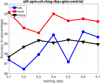
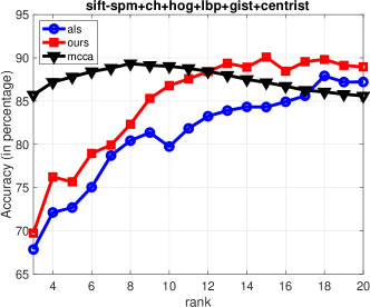
(a)	(b)

Figure 1. Sensitivity analysis of compared methods with six views on data Caltech101-7. (a) varying the training ratios over common spaces from 3 to 20; (b) varying the size of common space on 30% training data.

6.2. Experiments on Caltech101-7

We tested the overall performance of three compared methods on Caltech101-7 with all combinations of more than two views. For six views, there are 42 combinations in total. This experiment is conducted on 30% training data and 70% testing data by running three compared methods on each combination separately with the size of the common space (or rank) varied from 3 to 20. The experiment is repeated 10 times on randomly splits drawn from the input data, and the mean accuracies with standard deviations of three compared methods are reported in Table 2.

Table 2. Mean accuracy and standard deviation of three compared methods on $42$ data sets generated from Caltech101-7 over $10$ random splits with 30% training data and rank $20$.

views	als	Alg. 5.1	mcca
centrist+gist+lbp	95.23 $\pm$ 0.69	95.30 $\pm$ 0.73	90.74 $\pm$ 0.88
centrist+gist+hog	95.26 $\pm$ 0.58	95.32 $\pm$ 0.46	90.28 $\pm$ 0.96
centrist+gist+ch	92.47 $\pm$ 2.21	93.86 $\pm$ 0.96	90.66 $\pm$ 1.25
centrist+gist+sift-spm	95.56 $\pm$ 0.75	95.93 $\pm$ 0.39	92.59 $\pm$ 0.84
centrist+lbp+hog	94.95 $\pm$ 0.63	95.19 $\pm$ 0.65	90.09 $\pm$ 0.75
centrist+lbp+ch	92.63 $\pm$ 0.56	92.97 $\pm$ 0.65	90.06 $\pm$ 1.04
centrist+lbp+sift-spm	94.82 $\pm$ 0.75	95.15 $\pm$ 0.71	91.59 $\pm$ 0.71
centrist+hog+ch	91.29 $\pm$ 1.14	92.62 $\pm$ 1.07	89.79 $\pm$ 0.68
centrist+hog+sift-spm	93.46 $\pm$ 1.34	93.86 $\pm$ 1.27	91.15 $\pm$ 0.55
centrist+ch+sift-spm	90.24 $\pm$ 1.83	92.29 $\pm$ 0.94	88.99 $\pm$ 0.33
gist+lbp+hog	95.49 $\pm$ 0.92	95.63 $\pm$ 0.82	90.25 $\pm$ 0.85
gist+lbp+ch	93.04 $\pm$ 1.11	93.99 $\pm$ 0.60	90.93 $\pm$ 1.29
gist+lbp+sift-spm	95.71 $\pm$ 1.16	96.02 $\pm$ 0.60	92.41 $\pm$ 0.92
gist+hog+ch	90.86 $\pm$ 1.74	91.87 $\pm$ 1.92	89.60 $\pm$ 0.74
gist+hog+sift-spm	93.02 $\pm$ 0.58	93.05 $\pm$ 0.52	91.03 $\pm$ 0.47
gist+ch+sift-spm	90.14 $\pm$ 2.19	92.73 $\pm$ 1.09	90.25 $\pm$ 0.86
lbp+hog+ch	91.65 $\pm$ 1.51	92.98 $\pm$ 1.12	89.88 $\pm$ 0.67
lbp+hog+sift-spm	93.18 $\pm$ 0.77	94.16 $\pm$ 1.10	91.21 $\pm$ 0.50
lbp+ch+sift-spm	90.48 $\pm$ 1.61	92.33 $\pm$ 1.10	89.09 $\pm$ 0.46
hog+ch+sift-spm	88.35 $\pm$ 3.82	91.93 $\pm$ 0.94	90.07 $\pm$ 0.87
centrist+gist+lbp+hog	92.14 $\pm$ 3.41	95.12 $\pm$ 1.03	89.14 $\pm$ 0.70
centrist+gist+lbp+ch	89.25 $\pm$ 2.64	92.41 $\pm$ 1.93	90.17 $\pm$ 0.87
centrist+gist+lbp+sift-spm	90.05 $\pm$ 3.10	94.60 $\pm$ 1.25	90.64 $\pm$ 0.88
centrist+gist+hog+ch	84.91 $\pm$ 4.33	93.01 $\pm$ 2.05	89.63 $\pm$ 0.53
centrist+gist+hog+sift-spm	88.32 $\pm$ 4.01	92.94 $\pm$ 0.81	90.42 $\pm$ 0.46
centrist+gist+ch+sift-spm	85.30 $\pm$ 3.53	92.90 $\pm$ 1.94	90.97 $\pm$ 0.63
centrist+lbp+hog+ch	87.09 $\pm$ 2.72	92.52 $\pm$ 1.78	89.29 $\pm$ 0.55
centrist+lbp+hog+sift-spm	87.00 $\pm$ 5.27	93.30 $\pm$ 2.36	89.82 $\pm$ 0.58
centrist+lbp+ch+sift-spm	84.64 $\pm$ 3.74	92.21 $\pm$ 1.96	89.21 $\pm$ 0.90
centrist+hog+ch+sift-spm	84.65 $\pm$ 3.19	92.31 $\pm$ 1.33	90.02 $\pm$ 0.51
gist+lbp+hog+ch	86.50 $\pm$ 6.35	92.76 $\pm$ 1.41	89.11 $\pm$ 0.38
gist+lbp+hog+sift-spm	87.96 $\pm$ 2.63	93.86 $\pm$ 1.21	89.96 $\pm$ 0.47
gist+lbp+ch+sift-spm	85.25 $\pm$ 3.50	91.93 $\pm$ 1.98	90.83 $\pm$ 0.60
gist+hog+ch+sift-spm	81.57 $\pm$ 5.98	90.82 $\pm$ 2.06	90.53 $\pm$ 0.54
lbp+hog+ch+sift-spm	83.20 $\pm$ 4.93	91.59 $\pm$ 1.65	89.89 $\pm$ 0.68
gist+lbp+hog+ch+sift-spm	84.38 $\pm$ 3.13	91.32 $\pm$ 2.46	89.76 $\pm$ 0.61
centrist+lbp+hog+ch+sift-spm	86.11 $\pm$ 3.49	91.80 $\pm$ 2.32	89.48 $\pm$ 0.73
centrist+gist+hog+ch+sift-spm	86.67 $\pm$ 4.70	92.51 $\pm$ 1.11	90.12 $\pm$ 0.60
centrist+gist+lbp+ch+sift-spm	88.70 $\pm$ 3.73	93.07 $\pm$ 1.35	89.96 $\pm$ 0.87
centrist+gist+lbp+hog+sift-spm	85.31 $\pm$ 4.66	94.17 $\pm$ 1.37	89.25 $\pm$ 0.47
centrist+gist+lbp+hog+ch	85.75 $\pm$ 4.66	92.48 $\pm$ 2.10	89.00 $\pm$ 0.49
sift-spm+ch+hog+lbp+gist+centrist	87.91 $\pm$ 2.98	90.09 $\pm$ 2.95	89.33 $\pm$ 0.65

From Table 2, we have the following observations: (i) als outperforms mcca on three views, but underperforms mcca for more than three views; (ii) Our method outperforms both als and mcca consistently over all 42 combinations. These results imply that tensor-based methods can outperform mcca, when a good tensor approximation solver like our proposed algorithm is applied.

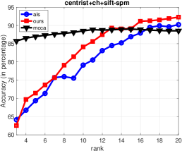
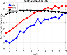
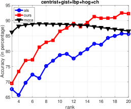
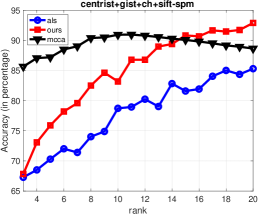
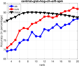
Figure 2. Experimental results of compared methods on Caltech101-7 with three, four and five views over 30% training data.

We further investigate the impact of compared methods in terms of the varied ranks and the training ratios. In Figure 1(a), the mean accuracy of testing data obtained by three compared methods varies when the training ratio increases from 10% to 70%. Due to the complexity of the tensor approximation problem, both als and our method show larger fluctuations than that of mcca when the training ratio increases. However, our method consistently outperforms both als and mcca over all tested training ratios. In Figure 1(b), we show the mean accuracy of compared methods on 10 random splits with 30% training data by varying rank from 3 to 20 on six views. In addition, we show the mean accuracy of compared methods on varied ranks on 30% with respect to combinations of different views in Figure 2. All these results demonstrate a similar trend with respect to testing accuracy when the rank increases from 3 to 20: mcca shows better performance on small ranks, but our method outperforms both mcca and als on large ranks, and overall our method obtains the best performance over all tested ranks. From Figure 1, we can see that our model on 30% training data shows the worst results comparing to other training ratios. This implies that the results in Figure 1 show the worst results of our method, which still outperforms the other two methods as shown in Figure 2. Moreover, we report the empirical comparison of computational time for these three methods, according to values of ranks and views on Caltech101-7. The comparison is shown in Table 3. For cleanness, the average CPU time over the combinations of fixed numbers of views is reported. As the experiments show, mcca is the fastest one, because the generalized eigenvalue decomposition for matrices of size $20\times v$ ($v\in\{3,4,5,6\}$) can be very fast. Our method is slower than mcca and als. As the number of views increases, the size of tensor increases and our method becomes slower.

Table 3. The CPU time of three compared methods on Caltech101-7 in terms of both ranks and views.

rank	3 views			4 views			5 views
	mcca	als	Alg. 5.1	mcca	als	Alg. 5.1	mcca	als	Alg. 5.1
3	0.0016	0.0464	0.0578	0.0022	0.0520	0.0863	0.0040	0.2463	0.7044
4	0.0013	0.0450	0.0656	0.0022	0.0517	0.0916	0.0037	0.2388	0.8510
5	0.0014	0.0464	0.0713	0.0021	0.0537	0.1216	0.0040	0.2434	1.0633
6	0.0013	0.0459	0.0781	0.0021	0.0522	0.1431	0.0041	0.2461	1.2318
7	0.0013	0.0464	0.0797	0.0022	0.0537	0.1519	0.0036	0.2435	1.3059
8	0.0013	0.0478	0.0843	0.0020	0.0520	0.1578	0.0037	0.2563	1.3738
9	0.0014	0.0454	0.0942	0.0022	0.0536	0.1665	0.0035	0.2556	1.4235
10	0.0013	0.0461	0.0961	0.0023	0.0528	0.1778	0.0036	0.2609	1.6305

6.3. Experiments on Scene15

The experiments same as in section 6.2 are performed on data Scene15. In Table 4, tensor-based methods including both als and ours outperform mcca on all view combinations. Our method outperforms als on three and four views, while it is competitive to als on five views. Figure 3 demonstrates the sensitivity of compared methods by varying the rank and the training ratios. On data Scene15, the tensor-based methods are consistently better than mcca over all tested training ratios, while our method outperforms als on large ranks and is competitive on small ranks. These results are consistent with the observations on Caltech101-7 in section 6.2, especially on relatively large ranks.

Table 4. Mean accuracy and standard deviation of two compared methods on $16$ data sets generated from Scene15 over $10$ random splits with 30% training data and rank $20$.

views	als	ours	mcca
centrist+gist+lbp	65.91 $\pm$ 1.45	66.66 $\pm$ 1.12	57.01 $\pm$ 0.81
centrist+gist+hog	67.21 $\pm$ 1.15	67.73 $\pm$ 1.08	58.47 $\pm$ 0.88
centrist+gist+sift-spm	70.40 $\pm$ 1.48	72.68 $\pm$ 1.70	64.34 $\pm$ 1.65
centrist+lbp+hog	60.29 $\pm$ 1.80	62.32 $\pm$ 1.56	53.63 $\pm$ 0.72
centrist+lbp+sift-spm	60.30 $\pm$ 1.83	65.43 $\pm$ 1.45	58.10 $\pm$ 1.46
centrist+hog+sift-spm	63.05 $\pm$ 1.98	67.45 $\pm$ 1.24	58.11 $\pm$ 1.24
gist+lbp+hog	61.08 $\pm$ 1.33	62.86 $\pm$ 1.20	54.20 $\pm$ 0.74
gist+lbp+sift-spm	65.82 $\pm$ 1.68	68.88 $\pm$ 1.30	59.23 $\pm$ 1.42
gist+hog+sift-spm	63.12 $\pm$ 3.94	67.13 $\pm$ 2.28	54.71 $\pm$ 1.76
lbp+hog+sift-spm	57.08 $\pm$ 2.54	60.58 $\pm$ 1.32	51.01 $\pm$ 2.05
centrist+gist+lbp+hog	62.33 $\pm$ 2.21	63.83 $\pm$ 2.11	51.07 $\pm$ 0.72
centrist+gist+lbp+sift-spm	61.96 $\pm$ 3.02	65.34 $\pm$ 1.62	55.56 $\pm$ 1.08
centrist+gist+hog+sift-spm	62.41 $\pm$ 3.08	63.67 $\pm$ 3.70	58.69 $\pm$ 1.19
centrist+lbp+hog+sift-spm	54.63 $\pm$ 3.26	57.98 $\pm$ 2.37	51.77 $\pm$ 1.57
gist+lbp+hog+sift-spm	58.93 $\pm$ 3.18	61.28 $\pm$ 2.26	50.05 $\pm$ 1.15
centrist+gist+lbp+hog+sift-spm	60.72 $\pm$ 2.87	60.35 $\pm$ 3.33	49.11 $\pm$ 1.49

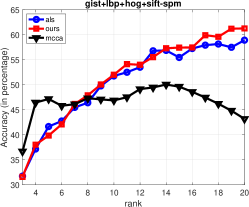
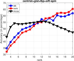
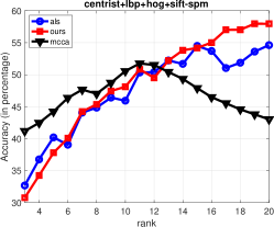
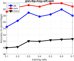
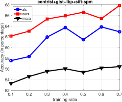
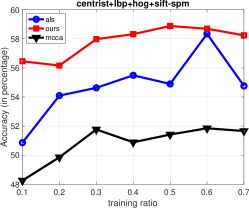
Figure 3. Sensitivity analysis of compared methods with four views on data Scene15. (top row) varying the size of common space on 30% training data; (bottom row) varying the training ratios over common spaces from 3 to 20.

Acknowledgement The first author is partially supported by the NSF grant DMS-2110780. The second author is partially supported by the NSF grant DMS-2009689.

References

- [1] Galen Andrew, Raman Arora, Jeff Bilmes, and Karen Livescu. Deep canonical correlation analysis. In International Conference on Machine Learning, pages 1247–1255. PMLR, 2013.
- [2] Giuseppe Brandi, Ruggero Gramatica, and Tiziana Di Matteo. Unveil stock correlation via a new tensor-based decomposition method. Journal of Computational Science, 46, 101116, 2020.
- [3] Paul Breiding and Nick Vannieuwenhoven. A Riemannian trust region method for the canonical tensor rank approximation problem, SIAM Journal on Optimization, 28(3), 2435–2465, 2018.
- [4] Chih-Chung Chang and Chih-Jen Lin. Libsvm: a library for support vector machines. ACM Transactions on Intelligent Systems and Technology (TIST), 2(3), 1–27, 2011.
- [5] Pierre Comon. Tensor decompositions, state of the art and applications. arXiv preprint arXiv:0905.0454, 2009.
- [6] Pierre Comon and Lek-Heng Lim. Sparse representations and low-rank tensor approximation. 2011.
- [7] Chun-Feng Cui, Yu-Hong Dai, Jiawang Nie, All real eigenvalues of symmetric tensors. SIAM Journal on Matrix Analysis and Applications, 35(4), 1582–1601, 2014.
- [8] Nguyen Thi Anh Dao, Nguyen Viet Dung, Nguyen Linh Trung, Karim Abed-Meraim, et al. Multi-channel eeg epileptic spike detection by a new method of tensor decomposition. Journal of Neural Engineering, 17(1), 016023, 2020.
- [9] Ian Davidson, Sean Gilpin, Owen Carmichael, and Peter Walker. Network discovery via constrained tensor analysis of fmri data. In Proceedings of the 19th ACM SIGKDD International Conference on Knowledge Discovery and Data Mining, pages 194–202, 2013.
- [10] Lieven De Lathauwer, A link between the canonical decomposition in multilinear algebra and simultaneous matrix diagonalization. SIAM Journal on Matrix Analysis and Applications, 28(3), 642–666, 2006.
- [11] Lieven De Lathauwer, Bart De Moor, and Joos Vandewalle. A multilinear singular value decomposition. SIAM Journal on Matrix Analysis and Applications, 21(4), 1253-1278, 2000.
- [12] Lieven De Lathauwer, Bart De Moor, and Joos Vandewalle, Computation of the canonical decomposition by means of a simultaneous generalized Schur decomposition. SIAM Journal on Matrix Analysis and Applications, 26(2), 295–327, 2004.
- [13] Lieven De Lathauwer, Bart De Moor, and Joos Vandewalle. On the best rank-1 and rank- approximation of higher-order tensors. SIAM Journal on Matrix Analysis and Applications, 21(4), 1324–1342, 2000.
- [14] Ignat Domanov and Lieven De Lathauwer. Canonical polyadic decomposition of third-order tensors: Reduction to generalized eigenvalue decomposition. SIAM Journal on Matrix Analysis and Applications, 35(2), 636–660, 2014.
- [15] Jinyan Fan, Jiawang Nie and Anwa Zhou, Tensor eigenvalue complementarity problems. Mathematical Programming, 170(2), 507–539, 2018.
- [16] Shmuel Friedland and Giorgio Ottaviani. The number of singular vector tuples and uniqueness of best rank-one approximation of tensors. Foundations of Computational Mathematics, 14(6), 1209–1242, 2014.
- [17] Yu Guan, Moody T Chu, and Delin Chu. Convergence analysis of an svd-based algorithm for the best rank-1 tensor approximation. Linear Algebra and its Applications, 555, 53–69, 2018.
- [18] Bingni Guo, Jiawang Nie, and Zi Yang. Learning diagonal gaussian mixture models and incomplete tensor decompositions. Vietnam Journal of Mathematics, to appear, 2021.
- [19] David R Hardoon and John Shawe-Taylor. Sparse canonical correlation analysis. Machine Learning, 83(3), 331–353, 2011.
- [20] Hotelling Harold. Relations between two sets of variates. Biometrika, 28(3/4):321–377, 1936.
- [21] Christopher J Hillar and Lek-Heng Lim. Most tensor problems are np-hard. Journal of the ACM (JACM), 60(6), 1–39, 2013.
- [22] Ian T. Jolliffe Principal Component Analysis. Springer Series in Statistics. New York: Springer-Verlag. 2002.
- [23] Tamara G. Kolda and Brett W. Bader. Tensor decompositions and applications. SIAM Review, 51(3), 455–500, September 2009.
- [24] Joseph Landsberg, Tensors: Geometry and Applications, Grad. Stud. Math., Providence, 2012.
- [25] Brett W. Larsen and Tamara G. Kolda. Practical leverage-based sampling for low-rank tensor decomposition, 2020.
- [26] Svetlana Lazebnik, Cordelia Schmid, and Jean Ponce. Beyond bags of features: Spatial pyramid matching for recognizing natural scene categories. In 2006 IEEE Computer Society Conference on Computer Vision and Pattern Recognition (CVPR’06), pages 2169–2178. IEEE, 2006.
- [27] Fei-Fei Li, Rob Fergus, and Pietro Perona. Learning generative visual models from few training examples: An incremental bayesian approach tested on 101 object categories. Computer Vision and Image Understanding, 106(1), 59–70, 2007.
- [28] Lek-Heng Lim, Tensors and hypermatrices, in: L. Hogben (Ed.), Handbook of linear algebra, 2nd Ed., CRC Press, Boca Raton, 2013.
- [29] Yong Luo, Dacheng Tao, Kotagiri Ramamohanarao, Chao Xu, and Yonggang Wen. Tensor canonical correlation analysis for multi-view dimension reduction. IEEE transactions on Knowledge and Data Engineering, 27(11), 3111–3124, 2015.
- [30] Jiawang Nie. Generating polynomials and symmetric tensor decompositions. Foundations of Computational Mathematics, 17(2), 423–465, 2017.
- [31] Jiawang Nie. Low rank symmetric tensor approximations. SIAM Journal on Matrix Analysis and Applications, 38(4), 1517–1540, 2017.
- [32] Jiawang Nie and Li Wang. Semidefinite relaxations for best rank-1 tensor approximations. SIAM Journal on Matrix Analysis and Applications, 35(3),1155–1179, 2014.
- [33] Jiawang Nie and Zi Yang. Hermitian tensor decompositions. SIAM Journal on Matrix Analysis and Applications, 41(3), 1115–1144, 2020.
- [34] Jiawang Nie, Zi Yang and Xinzhen Zhang. A complete semidefinite algorithm for detecting copositive matrices and tensors. SIAM Journal on Optimization, 28(4), 2902–2921, 2018.
- [35] Allan Aasbjerg Nielsen. Multiset canonical correlations analysis and multispectral, truly multitemporal remote sensing data. IEEE Transactions on Image Processing, 11(3), 293–305, 2002.
- [36] Aude Oliva and Antonio Torralba. Modeling the shape of the scene: A holistic representation of the spatial envelope. International Journal of Computer Vision, 42(3), 145–175, 2001.
- [37] Timo Ojala, Matti Pietikäinen, and Topi Mäenpää. Multiresolution gray-scale and rotation invariant texture classification with local binary patterns. IEEE Transactions on Pattern Analysis and Machine Intelligence, 24(7), 971–987, 2002.
- [38] Anh-Huy Phan, Petr Tichavskỳ, and Andrzej Cichocki. Fast alternating ls algorithms for high order candecomp/parafac tensor factorizations. IEEE Transactions on Signal Processing, 61(19), 4834–4846, 2013.
- [39] Laurent Sorber, Marc Van Barel, and Lieven De Lathauwer. Optimization-based algorithms for tensor decompositions: canonical polyadic decomposition, decomposition in rank- terms and a new generalization, SIAM Journal on Optimization, 23(2), 695–720, 2013.
- [40] Viivi Uurtio, João M Monteiro, Jaz Kandola, John Shawe-Taylor, Delmiro Fernandez-Reyes, and Juho Rousu. A tutorial on canonical correlation methods. ACM Computing Surveys (CSUR), 50(6), 1–33, 2017.
- [41] Nico Vervliet, Otto Debals, Laurent Sorber, Marc Van Barel, and Lieven De Lathauwer. Tensorlab 3.0, March 2016.
- [42] Javier Vía, Ignacio Santamaría, and Jesús Pérez. A learning algorithm for adaptive canonical correlation analysis of several data sets. Neural Networks, 20(1), 139–152, 2007.
- [43] Jianixn Wu and James M Rehg. Where am i: Place instance and category recognition using spatial pact. In 2008 Ieee Conference on Computer Vision and Pattern Recognition, pages 1–8. IEEE, 2008.
- [44] Xinghao Yang, Liu Weifeng, Wei Liu, and Dacheng Tao. A survey on canonical correlation analysis. IEEE Transactions on Knowledge and Data Engineering, 33(6), 2349–2368, 2021.