Elliptic Harnack Inequality for $\mathbb{Z}^{d}$

Abstract

We prove the scale invariant Elliptic Harnack Inequality (EHI) for non-negative harmonic functions on $\mathbb{Z}^{d}$. The purpose of this note is to provide a simplified self-contained probabilistic proof of EHI in $\mathbb{Z}^{d}$ that is accessible at the undergraduate level. We use the Local Central Limit Theorem for simple symmetric random walks on $\mathbb{Z}^{d}$ to establish Gaussian bounds for the $n$-step probability function. The uniform Green inequality and the classical Balayage formula then imply the EHI.

AMS 2010 Subject Classification : Primary: 05C81 Secondary: 31C05, 31C20
Keywords : Random walk, Harmonic Function, Harnack Inequality, Gaussian Bounds, Balayage.

1 Introduction

The scale invariant Elliptic Harnack Inequality (EHI) and its applications to the theory of elliptic and parabolic partial differential equations are well known. The work on regularity of solutions dates back to 1950’s in the works of de Giorgi [DG57], Nash [Nas58] and Moser [Mos61]. Moser first proved EHI for solutions to partial differential equations in divergence form in $\mathbb{R}^{d}$. Bombieri-Giusti [BG72] showed that EHI holds for minimal surfaces and EHI was proven for metric spaces by Sturm [Stu98]. We refer the interested reader to the survey article by Kassmann [Kas07], and the references therein for a comprehensive review of the Harnack inequality (for elliptic and parabolic operators) in $\mathbb{R}^{d}$.

The EHI was established for weighted graphs by Delmotte [Del99]. Barlow [Bar17] has a comprehensive treatment of random walks on locally finite graphs and in [Bar17, Theorem 7.19] presents a proof of EHI for weighted graphs that have controlled weights and are roughly isometric to $\mathbb{Z}^{d}$. In this short note our aim is to provide a simplified self-contained probabilistic proof of EHI for harmonic functions on $\mathbb{Z}^{d}$ using properties of the simple symmetric random walk. Lawler in [Law13, Theorem 1.7.2] also provides a proof of EHI for $\mathbb{Z}^{d}$. In this short note our aim is to provide a simplified self-contained probabilistic proof of EHI for harmonic functions on $\mathbb{Z}^{d}$ following the framework laid out in [Bar17] using properties of the simple symmetric random walk.

Let $d\geq 1$ and $\mathbb{Z}^{d}$ be the integer lattice. We will think of $\mathbb{Z}^{d}$ as a graph with vertex set

$$\mathbb{Z}^{d}=\{(x_{i})_{i=1}^{d}:x_{i}\in\mathbb{Z}\}$$

endowed with the (graph) distance $d(x,y)=\sum_{i=1}^{d}|x_{i}-y_{i}|$ between any two points $x,y\in\mathbb{Z}^{d}$. We may view edge set $E=\{\{x,y\}:x,y\in V,\,d(x,y)=1\}.$ For any $x,y\in\mathbb{Z}^{d}$ we shall say $x\sim y$ if $\{x,y\}\in E$. For $r>0$, we define the ball of radius $r$ around a point $x_{0}\in\mathbb{Z}^{d}$ as

$$B(x_{0},r)=\{x\in\mathbb{Z}^{d}:d(x,x_{0})\leq r\}.$$

Let $A\subset\mathbb{Z}^{d}$. We define the boundary of $A\subset\mathbb{Z}^{d}$ by

$$\partial A=\{y\in A^{c}:\exists\,x\in A\mbox{ with }x\sim y\}$$

and set $\bar{A}=A\cup\partial A$. For $f:\bar{A}\rightarrow\mathbb{R}$ we define the Laplacian $\Delta$ of $f$ as

$$\Delta f(x)=\frac{1}{2d}\sum_{x\sim y}(f(x)-f(y)),\qquad\mbox{for all }x\in A.$$

A function $f:\bar{A}\rightarrow\mathbb{R}$ is said to be harmonic in $A$ if $\Delta f(x)=0$ for all $x\in A$. The scale invariant EHI is then stated as follows.

Theorem 1.1 (EHI).

Let $d\geq 1$. There exists $C$ such that for any $x_{0}\in\mathbb{Z}^{d}$, $R\geq 1$, $h:\overline{B(x_{0},R)}\rightarrow\mathbb{R}_{+}$ with $h$ harmonic in $B(x_{0},R)$ we have

$$\max_{y\in B\left(x_{0},\frac{R}{2}\right)}h(y)\leq C\min_{z\in B\left(x_{0},\frac{R}{2}\right)}h(z)$$ (1.1)

We work with simple symmetric random walks in $\mathbb{Z}^{d}$, whose transition probability matrix $P$ is connected with the Laplacian $\Delta$. The proof has three key steps – the Gaussian bounds for the $n$-step probability function of the simple symmetric random walk (Proposition 2.1), the uniform Green inequality for the Green function asssociated with the random walk (Proposition 2.2), and the Balayage formula for harmonic functions (Proposition 2.3).

The proof of Theorem 1.1 that we present here proceeds along the framework given in the proof of [Bar17, Theorem 7.19] (which applies for those graphs which have controlled weights and are roughly isometric to $\mathbb{Z}^{d}$). Our proof uses methods specific to the random walk on $\mathbb{Z}^{d}$ and has appropriate simplifications whenever possible. To establish Proposition 2.1 for weighted graphs one first shows the Poincaré inequality along with a growth condition for volume of the balls in the graph. Then the equivalence results shown in [Del99] will imply the result (See also [Bar17, Theorem 6.28]). For $\mathbb{Z}^{d}$, we use the Local Central Limit Theorem for simple random walks to obtain near diagonal bounds on the $n$-step transition probability function (See Proposition 3.2). Then the Gaussian lower bound is obtained via a classical chaining of balls argument. The Gaussian upper bound follows from exponential bounds for the distribution of exit times of the simple random walk from a ball. For this, we use the specific structure of the walk in $\mathbb{Z}^{d}$, by reducing the question for the $d$ dimensional random walk to a one dimensional walk which follow from Chernoff bounds (See Lemma 3.3). We also note that Gaussian bounds for the simple symmetric random walk in $\mathbb{Z}^{d}$ are part of folklore and are well known but it is hard to point to explicit references in the literature where they can be found.

As mentioned before, [Law13, Theorem 1.7.2] also contains a proof for the EHI in $\mathbb{Z}^{d}$. There the uniform Green inequality is obtained using explicit bounds on the hitting distribution of the walk for three and higher dimensions [Law13, Proposition 1.5.10] and on the Green function for two dimensions in [Law13, Proposition 1.6.7]. The Local Central Limit Theorem is used to derive precise asymptotics on the Green function and the propositions are proved via an application of the optional stopping theorem for martingales. For proving the uniform Green inequality we use Proposition 2.1 to establish Gaussian bounds for $n$-step transition probabilities of walk killed on exiting the ball. Plugging these estimates and exit time bounds obtained above into the definition of the Green function one obtains the result. The Balayage formula is shown using the probabilistic representation for the solution to the Dirichlet problem and standard potential theory techniques. The proofs of uniform Green inequality and the Balayage formula translate to graphs that have controlled weights and are roughly isometric to $\mathbb{Z}^{d}$ (See [Bar17, Theorem 4.26, Theorem 7.15]).

The Balayage formula is analogous to the classical Poisson integral formula for Harmonic functions in $\mathbb{R}^{d}$ with the Green function playing the role of the Poisson Kernel. The uniform Green inequality then enables the scale invariant Harnack inequality. The uniform Green inequality are implied by the Gaussian bounds.

We remark that the constant $C$ in Theorem 1.1 does not depend on $R$ but only on dimension $d$ and the $\frac{1}{2}$-scaling used to obtain the smaller ball. There are many applications of the EHI. For instance, using EHI one can show that the probability of exiting the boundary of $B(x_{0},R)$ via a particular set is comparable for different starting points inside $B(x_{0},\frac{R}{2}$). The EHI implies the oscillation inequality for harmonic functions, in the sense that if for any set $A\subset\mathbb{Z}^{d},$

$$\mbox{Osc}(h,A)=\sup_{x\in A}h(x)-\inf_{x\in A}h(x)$$

then there is a $0<\delta<1$ such that

$$\mbox{Osc}\left(h,B\left(x_{0},\frac{R}{2}\right)\right)\leq(1-\delta)\mbox{Osc}\left(h,B(x_{0},R)\right).$$

The oscillation inequality will then imply Hölder continuity for $h$ and more importantly the Strong Liouville property, which asserts that if $h\geq 0$ and is harmonic on $\mathbb{Z}^{d}$ then $h$ is constant (See [Bar17, Theorem 1.46]).

Acknowledgements: We would like to thank Martin Barlow and D. Yogeshwaran for useful discussions and feedback on a draft of the note. We also thank Greg Lawler for pointing us to [Law13, Theorem 1.7.2]. This work was done as part of a summer reading seminar when Nitya Gadhiwala and Ritvik Radhakrishnan were undergraduate students in the B. Math. (Hons.) program at the Indian Statistical Institute, Bangalore centre. Siva Athreya was partially supported by a CPDA grant at the Indian Statistical Institute, Bangalore centre.

Layout for rest of the paper: In Section 2 we will prove Theorem 1.1 assuming the three Propositions. Then we prove the Gaussian bounds in Section 3, the uniform Green inequality in Section 4, and the Balayage formula in Section 5, to complete the proof.

Convention on constants. Throughout the article $c,c_{1},c_{2},\ldots$ denote positive constants whose value may change from line to line. They are all positive and their precise values are not important. In statements of results will use capital letters $A,B,\ldots$ to denote special constants. Also, throughout this note the constants depend on the dimension $d$, but will not be mentioned explicitly. Any other dependence will be stated.

2 Proof of Theorem 1.1

When $d=1$, it is easy to see that any harmonic function $h:\mathbb{Z}\rightarrow\mathbb{R}$ is of the form $h(k)=\alpha k+\beta$ for some real numbers $\alpha,\beta.$ Then (1.1) follows immediately. We will now present a proof when $d\geq 2.$

Let $X$ be the simple random walk on $\mathbb{Z}^{d}$. That is, $X$ is a discrete time Markov chain $(\{X_{n}\}_{n\geq 0},\{\mathbb{P}^{x}\}_{x\in\mathbb{Z}^{d}})$ with transition matrix $P=[p_{xy}]$ given by

$$p_{xy}=\left\{\begin{array}[]{ll}\frac{1}{2d}&\mbox{ if }x\sim y,\\ 0&\mbox{ otherwise,}\end{array}\right.$$

for any $x,y\in\mathbb{Z}^{d}$ on a measure space $(\Omega,{\cal F})$. Under the probability $\mathbb{P}^{x}$ we have $\mathbb{P}^{x}(X_{0}=x)=1$. Note that $\Delta=(P-I)$. For any $n\geq 1$, we will denote the $n$-step probability function of $X$ by

$$p_{n}(x,y)=\mathbb{P}^{x}(X_{n}=y),$$ (2.1)

with $p_{1}(x,y)=p_{xy}$. The first step in the proof is to establish the following Gaussian upper and lower bounds for the $n$-step probabilities of the random walk.

Proposition 2.1 (Gaussian Bounds).

Let $X_{n}$ be the simple random walk on $\mathbb{Z}^{d}$ with $n$-step probability function $p_{n}(\cdot,\cdot)$ given by (2.1). Then

1. there exists $L_{1}>0$ and $L_{2}>0$ such that for all $x,y\in\mathbb{Z}^{d},n\geq\max\{1,d(x,y)\}$

   $$p_{n}(x,y)+p_{n+1}(x,y)\geq\frac{L_{1}}{n^{\frac{d}{2}}}\exp\left(-L_{2}\frac{d^{2}(x,y)}{n}\right),$$ (2.2)

2. there exists $U_{1}>0$ and $U_{2}>0$ such that for all $x,y\in\mathbb{Z}^{d},n\geq 0$

   $$p_{n}(x,y)\leq\frac{U_{1}}{(\max\{n,1\})^{\frac{d}{2}}}\exp\left(-U_{2}\frac{d^{2}(x,y)}{\max\{n,1\}}\right).$$ (2.3)

The second step in the proof is to use the Gaussian bounds to establish the Uniform Green Inequality. Now, for any subset $D\subset\mathbb{Z}^{d}$ define the entrance time to $D$ and exit time from $D$

$$T_{D}=\inf\{k\geq 0:X_{k}\in D\}\text{ and }\tau_{D}=\inf\{k\geq 0:X_{k}\in D^{c}\}.$$

We define the killed $n$-step probability function of $X$ by

$$p^{D}_{n}(x,y)=\mathbb{P}^{x}(X_{n}=y,n<\tau_{D}).$$ (2.4)

The Green function corresponding to $D$, $g_{D}:D\times D\rightarrow\mathbb{R}$, is given by

$$g_{D}(x,y)=\sum_{n=0}^{\infty}p_{n}^{D}(x,y).$$ (2.5)

Thus the Green function represents the expected time spent (or number of visits) by the walk at vertex $y$ before exiting the domain $D$ when it starts at $x$. We now state the Uniform Green Inequality.

Proposition 2.2 (Uniform Green Inequality).

There exists $G_{1},$ $G_{2}>0$ such that if $R\geq 2,B=B(x_{0},R),x,y\in B(x_{0},\frac{R}{2})$, $r=\max\{1,d(x,y)\}$, then

1. for $d\geq 3$

   $$\frac{G_{1}}{r^{d-2}}\leq g_{B}(x,y)\leq\frac{G_{2}}{r^{d-2}},$$ (2.6)

2. and for $d=2$

   $$G_{1}\log\left(\frac{R}{r}\right)\leq g_{B}(x,y)\leq G_{2}\log\left(\frac{R}{r}\right).$$ (2.7)

The uniform Green inequality is a key tool in the proof of EHI due to the fact that Green function plays a role similar to that of the Poisson Kernel for harmonic functions in $\mathbb{R}^{d}$. This established by the Balayage formula for harmonic functions. To state the result, we need one additional notation. For any $A\subset\mathbb{Z}^{d}$, we define the interior boundary of $A$ by

$$\partial_{i}A=\{y\in A:\exists\,x\in A^{c}\mbox{ with }x\sim y\}.$$

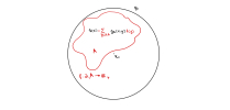
Figure 1: (Balayage Formula) For harmonic function $h:B\rightarrow R$ and a $A\subset B$ one can find a $f:\partial_{i}A\rightarrow\mathbb{R}$ such that $h$ is a weighted sum of $f$ in $A$ with the weights given by the Green function.

Proposition 2.3 (Balayage formula).

Let $R\geq 1$, $x_{0}\in V$, $B=B(x_{0},R),A\subsetneq B$. Assume $h:\overline{B}\rightarrow\mathbb{R}_{+}$ with $h$ being harmonic in $B.$ Then there exist $f:\partial_{i}A\rightarrow\mathbb{R}_{+}$ such that

$$h(x)=\sum_{y\in\partial_{i}A}g_{B}(x,y)f(y)\,\quad\forall\,x\in A$$ (2.8)

Assuming the above Propositions we are now ready to prove the main result. The proof is essentially an application of the Balayage formula and the uniform Green inequality, followed by a standard chaining of balls argument in $\mathbb{Z}^{d}$.

Proof of Theorem 1.1.

We will first consider the case when $R\leq 32$. For $x,y\in B(x_{0},\frac{R}{2})$ such that $x\sim y$ we have

$$h(x)=\sum_{z\sim x}\frac{1}{2d}h(z)\geq\frac{1}{2d}h(y).$$ (2.9)

Now for arbitary $x_{1},x_{2}\in B(x_{0},\frac{R}{2})$ there exists $z_{1},z_{2},\ldots z_{k}$ such that $x_{1}\sim z_{1}\sim z_{2}\ldots z_{k}\sim y$ with $k\leq 32.$ Using (2.9), we have that

$$h(x_{1})\geq\frac{1}{(2d)^{k}}h(x_{2})\geq\frac{1}{(2d)^{32}}h(x_{2}).$$

As $x_{1},x_{2}$ were arbitrary,

$$\max_{y\in B\left(x_{0},\frac{R}{2}\right)}h(y)\leq(2d)^{32}\min_{z\in B\left(x_{0},\frac{R}{2}\right)}h(z).$$ (2.10)

Thus proving (1.1) whenever $R\leq 32$. We shall now assume $R>32$. Set $B=B(x_{0},R),A=B\left(x_{0},\frac{R}{2}\right).$ Let $x_{1},x_{2}\in B\left(x_{0},\frac{R}{4}\right)$ and $y\in\partial_{i}A$. Firstly,

$$\frac{R}{4}\leq d(x_{i},y)\leq\frac{3R}{4}\qquad\mbox{for $i=1,2$}.$$

Applying Proposition 2.2, by (2.7) or (2.6), we have that

$$g_{B}(x_{1},y)\leq\frac{3^{d-2}G_{1}}{G_{2}}g_{B}(x_{2},y)\qquad\mbox{ for all }y\in\partial_{i}(A).$$ (2.11)

Using (2.8) from Proposition 2.3, we have that there exists $f$ supported on $\partial_{i}A$ such that

$$h(x)=\sum_{y\in\partial_{i}A}g_{B}(x,y)f(y)\,\quad\forall\,x\in A.$$

Applying (2.11) in the above we have that

$$h(x_{1})=\sum_{y\in\partial_{i}A}g_{B}(x_{1},y)f(y)\leq\frac{3^{d-2}G_{1}}{G_{2}}\sum_{y\in\partial_{i}A}g_{B}(x_{2},y)f(y)=\frac{3^{d-2}G_{1}}{G_{2}}h(x_{2}).$$ (2.12)

whenever $x_{1},x_{2}\in B(x_{0},\frac{R}{4}).$ To complete the proof we use a standard chaining of balls argument. As $R>32$, it is easy to see that there exists $N\geq 1$ such that for all $u,v\in B(x_{0},\frac{R}{2})$ there exists $z_{1},z_{2},\ldots,z_{N}\in B(x_{0},\frac{R}{2})$ such that

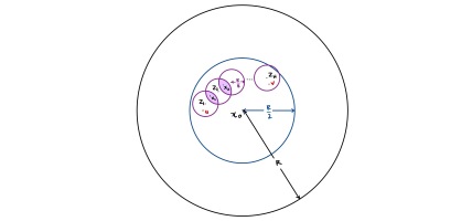
Figure 2: Figure depicts that standard chain of balls argument used in the proof of Theorem 1.1.

$$u\in B\left(z_{1},\frac{R}{8}\right),\qquad v\in B\left(z_{N},\frac{R}{8}\right),\qquad\mbox{ and }\qquad B\left(z_{j},\frac{R}{8}\right)\cap B\left(z_{{j+1}},\frac{R}{8}\right)\neq\emptyset\mbox{ for $1\leq j\leq N-1.$}$$

Let us choose corresponding arbitrary points $x_{j}\in B(z_{j},\frac{R}{8})\cap B(z_{{j+1}},\frac{R}{8})$. Note that $B(z_{j},\frac{R}{2})\subset B(x_{0},R)$ for all $1\leq j\leq N-1$. Thus $h$ satisfies the hypothesis when $R$ is replaced by $\frac{R}{2}$ and $x_{0}$ is replaced by $z_{j}$. Applying (2.12) with $R$ replaced by $\frac{R}{2}$ and $x_{0}$ successively replaced by $z_{j}$ we have that

$$h(u)\leq\frac{3^{d-2}G_{1}}{G_{2}}h(x_{1})\leq\left(\frac{3^{d-2}G_{1}}{G_{2}}\right)^{2}h(x_{2})\leq\left(\frac{3^{d-2}G_{1}}{G_{2}}\right)^{3}h(x_{3})\leq\ldots\left(\frac{3^{d-2}G_{1}}{G_{2}}\right)^{N}h(v).$$

As $u,v$ were arbitary we have that,

$$\max_{y\in B\left(x_{0},\frac{R}{2}\right)}h(y)\leq\left(\frac{3^{d-2}G_{1}}{G_{2}}\right)^{N}\min_{z\in B\left(x_{0},\frac{R}{2}\right)}h(z).$$ (2.13)

We have thus established (1.1) whenever $R>32$. This completes the proof. ∎

3 Gaussian Bounds

In this section we prove Proposition 2.1 which provides Gaussian upper and lower bounds for the $n$-step probability function of the simple random walk. First we shall use the well known Local Central Limit Theorem to obtain bounds for the $n$-step probability function near the diagonal. Using this and a chaining of balls argument we will obtain the Gaussian lower bound. For the Gaussian upper bound, we use the near diagonal bounds obtained along with an application of Chernoff bound to a one-dimensional projection of the random walk.

3.1 Near diagonal bounds

The following is the version of the local central limit theorem we use. We shall say that $n$ and $z\in\mathbb{Z}^{d}$ have the same parity if $n+|z_{1}|+\cdots+|z_{d}|$ is even.

Theorem 3.1 (Local Central Limit Theorem).

Let $\{X_{n}\}_{n\geq 0}$ denote a simple symmetric random walk in $\mathbb{Z}^{d}$. There exists positive constants $A,B,C$ such that for all positive integers $n$ and points $x,y\in\mathbb{Z}^{d}$ we have

$$\left|p_{n}(x,y)-\frac{A}{n^{\frac{d}{2}}}\exp\left(-\frac{Bd(x,y)^{2}}{n}\right)\right|\leq\frac{C}{n^{\frac{d}{2}+1}},$$ (3.1)

whenever $n$ and $y-x$ have the same parity.

Proof.

We refer the reader to Theorem 1.2.1 in [Law13] for the proof (or for more detailed explanation of the same in [Gad20]). We note that the statement in [Law13] has $d(x,y)$ to be standard Euclidean metric namely $||\cdot||_{2}$. The above statement where $d(x,y)$ is the graph distance easily follows because we have $c_{1}||x-y||_{2}\leq d(x,y)\leq c_{2}||x-y||_{2}$ for some constants $c_{1}>0$ and $c_{2}>0$. ∎

Proposition 3.2 (Near diagonal bounds).

There exists $N_{1}>0$ such that for all $x,y\in\mathbb{Z}^{d},n\geq 0$

$$p_{n}(x,y)\leq\frac{N_{1}}{(\max\{n,1\})^{\frac{d}{2}}},$$ (3.2)

and there exists $N_{2}>0$ and $L\in(0,1)$ such that for all $x,y\in\mathbb{Z}^{d},n\geq\frac{1}{L^{2}}\max\{1,d^{2}(x,y)\}$

$$p_{n}(x,y)+p_{n+1}(x,y)\geq\frac{N_{2}}{n^{\frac{d}{2}}}.$$ (3.3)

Proof.

We first establish equation (3.2) assuming Theorem 3.1. Choose $x,y\in\mathbb{Z}^{d}$. We want to bound $p_{n}(x,y)=\mathbb{P}^{x}(X_{n}=y)$ from above. Using the Local Central Limit Theorem we get

$$p_{n}(x,y) \leq\frac{C}{n^{\frac{d}{2}+1}}+\frac{A}{n^{\frac{d}{2}}}\exp\left(-\frac{Bd(x,y)^{2}}{n}\right)\leq\frac{C+A}{n^{\frac{d}{2}}}.$$

Thus the proof of (3.2) is complete.

Next we show (3.3). Choose $x=(x_{1},\ldots,x_{d}),y=(y_{1},\ldots,y_{d})\in\mathbb{Z}^{d}$. We want find a lower bound for $p_{n}(x,y)+p_{n+1}(x,y)=\mathbb{P}^{x}(X_{n}=y)+\mathbb{P}^{x}(X_{n+1}=y)$. Since the simple random walk on $\mathbb{Z}^{d}$ has period $2$, exactly one of $p_{n}(x,y)$ and $p_{n+1}(x,y)$ will be nonzero. The first is nonzero if $n+|y_{1}-x_{1}|+\cdots+|y_{d}-x_{d}|$ is even and the second if it is odd, in which case, $n+1+|y_{1}-x_{1}|+\cdots+|y_{d}-x_{d}|$ is even. Let $m$ be either $n$ or $n+1$ such that $p_{m}(x,y)$ is nonzero, so that $m$ and $y-x$ have the same parity.

It suffices to show that there exists $c>0$ and $L\in(0,1)$ such that for all $x,y\in\mathbb{Z}^{d}$ and $n\geq\frac{1}{L^{2}}\max\{1,d^{2}(x,y)\}$, we have

$$p_{m}(x,y)\geq\frac{c}{n^{\frac{d}{2}}}.$$

Using the Local Central Limit Theorem we have

$$p_{m}(x,y) \geq\frac{A}{m^{\frac{d}{2}}}\exp\left(-\frac{Bd(x,y)^{2}}{m}\right)-\frac{C}{m^{\frac{d}{2}+1}}$$

$$\geq\frac{1}{n^{\frac{d}{2}}}\left(c_{1}\exp\left(-\frac{c_{2}d(x,y)^{2}}{n}\right)-\frac{c_{3}}{n}\right).$$ (3.4)

Now, let $n\geq\frac{1}{L^{2}}\max\{1,d^{2}(x,y)\}$, for some $L\in(0,1)$ that will be determined later. So we have $L^{2}\geq\frac{1}{n}\max\{1,d^{2}(x,y)\}$. Replacing this in (3.4) we get

$$p_{m}(x,y)\geq\frac{1}{n^{\frac{d}{2}}}\left(c_{1}\exp(-c_{2}L^{2})-c_{3}L^{2}\right)$$

Now choose $0<\delta<1$ such that for $0<L<\delta$ we have

$$c_{1}\exp(-c_{2}L^{2})>\frac{c_{1}}{2}\qquad\mbox{ and }\qquad c_{3}L^{2}<\frac{c_{1}}{4}.$$

So for $0<L<\delta$ we get

$$p_{m}(x,y)\geq\frac{c_{1}}{2n^{\frac{d}{2}}}.$$

The proof of (3.3) is complete. ∎

3.2 Lower Bound

To establish the Gaussian lower bound we consider three cases, divided according to how $R=d(x,y)$ compares with $n$. For the third case we apply a chaining argument, and for this we require the following estimate on the volume of a ball in $\mathbb{Z}^{d}$. Namely, there exists a constant $V_{1}\leq 2d$ such that for all $x_{0}\in\mathbb{Z}^{d}$ and $r\geq 1$ we have

$$\left|B(x_{0},r)\right|\geq V_{1}r^{d}.$$ (3.5)

The below proof follows the same structure as in the proof of [Bar17, Proposition 4.38].

Proof of Proposition 2.1(a).

Let $x,y\in\mathbb{Z}^{d},R=d(x,y)$ and let $L>0$ be as in (3.3).

Case 1: Let $R\leq n\leq\frac{2^{6}}{L^{2}}R$. Then,

$$p_{n}(x,y)+p_{n+1}(x,y)\geq\left(\frac{1}{2d}\right)^{n+1}\geq c_{1}\exp(-c_{2}n)\geq\frac{c_{1}}{n^{\frac{d}{2}}}\exp\left(-c_{3}\frac{R^{2}}{n}\right).$$

This implies (2.2).

Case 2: Let $n\geq\frac{R^{2}}{L^{2}}$. In this case (3.3) implies (2.2).

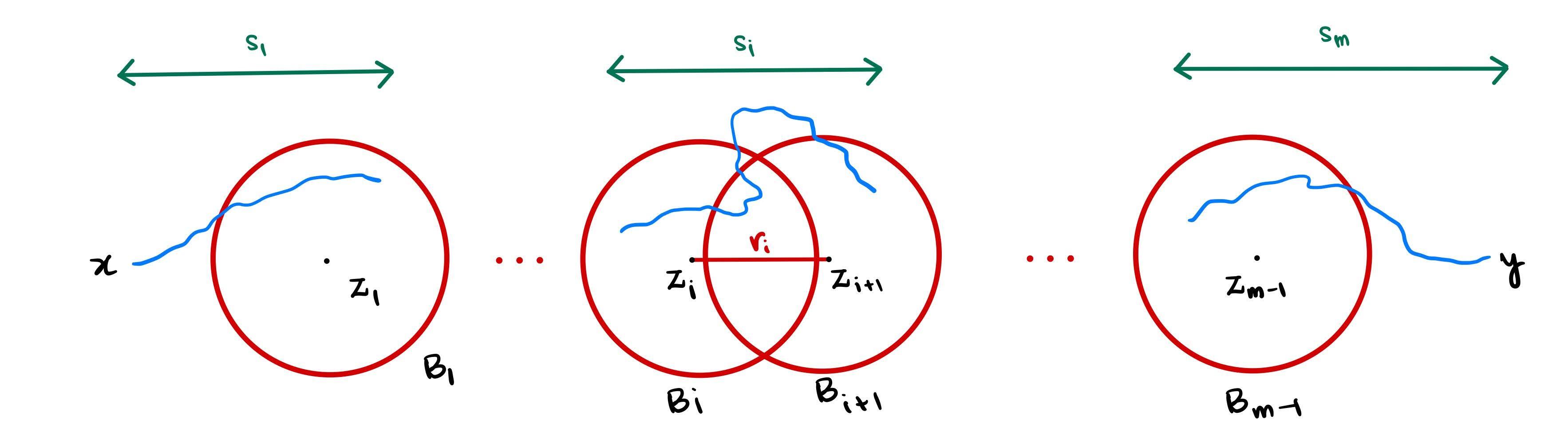
Figure 3: The basic idea of chaining of balls in the proof of Case 3 in Proposition 2.1(a) is to divide the random walk path into $m\approx\frac{R^{2}}{n}$ steps. This will imply that length of each segment $r_{i}$ above are approximately $\frac{R}{m}$, the time taken $s_{i}$ above are approximately $\frac{n}{m}$, and we can use (3.3) for each segment $i$, $1\leq i\leq m$ to obtain the result. The details of the proof ensures that there exists $m,r_{i},s_{i}$ are all natural numbers.

Case 3: Let $\frac{2^{6}}{L^{2}}R\leq n\leq\frac{R^{2}}{L^{2}}$. See Figure 3 for the basic idea of the chaining balls of argument used in the proof here. Given $n$ in this region choose $m\in\mathbb{N}$ such that

$$\frac{2^{5}R^{2}}{L^{2}n}\leq m\leq\frac{2^{6}R^{2}}{L^{2}n}.\\$$ (3.6)

Note that because $n\geq\frac{2^{6}}{L^{2}}R$, we have $1\leq m\leq R.$ Set $r=\lfloor\frac{R}{m}\rfloor$ and $s=\lfloor\frac{n}{m}\rfloor.$ Now, there exists

$$z_{1},z_{2},\ldots,z_{m} x=z_{0},\quad y=z_{m},\quad d(z_{i},z_{i+1})\in\{r,r+1\},$$:

and

$$s_{1},s_{2},\ldots,s_{m} s_{i}\in\{s,s+1\},\quad\sum_{i=1}^{m}s_{i}=n.$$:

Let $B_{i}=B(z_{i},r)$ for $0\leq i\leq m-2$. By considering all possible paths from $x$ to $y$ and the definition of $p_{n}$ we have that

$$p_{n}(x,y)+p_{n+1}(x,y)\geq\mathbb{P}^{x}(X_{s_{1}}\in B_{1})\cdot\prod_{i=1}^{m-2}\min_{w\in B_{i}}\mathbb{P}^{w}(X_{s_{i+1}}\in B_{i+1})\cdot\min_{w\in B_{m-1}}\mathbb{P}^{w}(X_{s_{m}}=y).$$

Next, by our choice of $m$, the lower bound in (3.6) implies that

$$(3r+1)^{2}\leq 16r^{2}\leq 16\frac{R^{2}}{m^{2}}\leq L^{2}\frac{n}{2m}\leq L^{2}s.$$ (3.7)

Since we have that $d(w,v)\leq 3r+1$ for all $w\in B_{i}$ and $v\in B_{i+1}$, the lower bound for $s$ in (3.7) implies that $s\geq\frac{1}{L^{2}}d(w,v)^{2}$. Hence from (3.3) we have that there exists $0<c_{1}<1$ such that

$$\min_{w\in B_{i}}\mathbb{P}^{w}(X_{s_{i+1}}\in B_{i+1})\geq\frac{c_{1}}{s^{\frac{d}{2}}}\qquad\mbox{for all}\qquad 0\leq i\leq m-2.$$ (3.8)

Using the volume bound from (3.5) and (3.8) in (3.2) we have

$$p_{n}(x,y) \geq \left(\frac{c_{1}V_{1}r^{d}}{\left(s_{1}\right)^{\frac{d}{2}}}\right)\quad\cdot\quad\prod_{i=1}^{m-2}\left(\frac{c_{1}V_{1}r^{d}}{\left(s_{i}\right)^{\frac{d}{2}}}\right)\quad\cdot\quad\left(\frac{c_{1}}{\left(s_{m}\right)^{\frac{d}{2}}}\right).$$ (3.9)

By our choice of $m$, the upper bound in (3.6) implies that

$$(16)^{2}r^{2}\geq(16)^{2}\frac{R^{2}}{4m^{2}}\geq 64L^{2}\frac{n}{64m}\geq L^{2}s.$$ (3.10)

Using (3.10), the fact that $s_{i}\geq s$ for all $1\leq i\leq m-1$, and $s_{m}\leq n$ in (3.9) we have

$$p_{n}(x,y)\geq\frac{c_{1}}{16^{d}}\left(\frac{c_{1}L^{d}V_{1}}{16^{d}}\right)^{m-1}\frac{1}{n^{\frac{d}{2}}}=\frac{c_{2}}{n^{\frac{d}{2}}}\exp(-c_{3}m)$$ (3.11)

for some $c_{2},c_{3}>0.$ Note that $c_{3}>0$ because $V_{1}\leq 2d$ from (3.5). Inserting the lower bound of $m$ from (3.6) in (3.11) implies (2.2).

∎

Remark 1.

The choice of the constant $\frac{2^{6}}{L^{2}}$ in Case 3 is not adhoc. One could derive it post-facto in the proof as well. To use the Local Central Limit Theorem in the chain of balls of argument we need a choice of $m$ such that

$$3r+1\leq L\sqrt{s}\leq 16r,$$   (see (3.10) and (3.7)).

This can be achieved if

$$4r\leq\frac{1}{L}\sqrt{\frac{n}{2m}}\mbox{ and }\frac{1}{L}\sqrt{\frac{n}{m}}\leq 8\frac{R}{m},$$

as $\frac{n}{2m}\leq s\leq\frac{n}{m}$ and $\frac{R}{2m}\leq r\leq\frac{R}{m}.$ This is possible if $m$ is an integer as in

$$\frac{2^{5}R^{2}}{L^{2}n}\leq m\leq\frac{2^{6}R^{2}}{L^{2}n},\qquad\mbox{ \em({\em see} \eqref{eq:cm}).}$$

This forces the choice of the constant in Case 3.

3.3 Upper Bound

Recall that, $B=B(x_{0},R)$ and $\tau_{B}=\inf\{k\geq 0:X_{k}\in B^{c}\}$. We note that $\tau_{B}$ is finite with probability one because

$$\mathbb{P}(\tau_{B}>n)\leq(1-p)^{\lfloor\frac{R}{n}\rfloor}$$ (3.12)

with (say) $p=(\frac{1}{2d})^{3R}$. We will need the following lemma for the proof of the upper bound.

Lemma 3.3.

$\mathbb{P}^{x}(\tau_{B}<n)\leq 2d\exp(-\frac{R^{2}}{4dn}).$

Proof.

We first reduce the question for the $d$ dimensional random walk to a one dimensional walk as follows. Without loss of generality we may assume $x_{0}=0$ and consider $B=B(0,R)$. Let $\{X_{n}\}_{n\geq 0}$ be the simple random walk on $\mathbb{Z}^{d}$ with $X_{0}=0$. Now, let $\{Y_{n}\}_{n\geq 0}$ be the lazy random walk on $\mathbb{Z}$, starting from $0$ with transition matrix given by $q$

$$q(u,v)=\left\{\begin{array}[]{ll}\frac{1}{2d}&\mbox{ if }u=v\pm 1,\\ &\\ \frac{d-1}{d}&\mbox{ if }u=v,\\ &\\ 0&\mbox{otherwise.}\end{array}\right.$$

Let $X_{n}(k)$ denote the $k$th coordinate of $X_{n}$ for $1\leq k\leq d$. Note that for each $k$, $\{X_{n}(k)\}_{n\geq 0}$ have the same distribution as $\{Y_{n}\}_{n\geq 0}$. Also, if $d(X_{n},0)>R$ then there is a coordinate $1\leq k\leq d$ for which $X_{n}(k)\geq\frac{R}{d}$, consequently using a union bound

$$\mathbb{P}(\tau_{B}\leq n)\leq d\mathbb{P}(\tau_{\frac{R}{d}}\leq n)$$ (3.13)

where $\tau_{S}=\inf\{k\geq 0:Y_{k}\not\in[-S,S]\}$ for any $S>0$.

We will understand $\tau_{S}$ for any $S=\frac{R}{d}$ and for that we define two auxiliary stopping times:

$$\tau_{S}^{+}=\left\{\begin{array}[]{ll}\tau_{S}&\mbox{ if }Y_{\tau_{S}}>0,\\ \infty&\mbox{ otherwise,}\end{array}\right.\qquad\mbox{ and }\qquad\tau_{S}^{-}=\left\{\begin{array}[]{ll}\tau_{S}&\mbox{ if }Y_{\tau_{S}}<0,\\ \infty&\mbox{ otherwise.}\end{array}\right.$$

Further it is easy to see that

$$\{\tau_{S}\leq n\}=\{\tau_{S}^{+}\leq n\}\dot{\cup}\{\tau_{S}^{+}\leq n\}$$

implying

$$\mathbb{P}(\tau_{S}\leq n)=\mathbb{P}(\tau_{S}^{+}\leq n)+\mathbb{P}(\tau_{S}^{-}\leq n).$$

We will estimate $\mathbb{P}(\tau_{S}^{+}\leq n)$ and the other term will follow similarly.

For $S\leq k\leq n,$ let $A_{k}=\{\tau^{+}_{S}=k\}.$ Note that $\mathbb{P}(A_{k})>0$ and

$$\{\tau_{S}^{+}\leq n\}=\cup_{k=S}^{n}A_{k}.$$

Note that,

$$\mathbb{E}[Y_{n}|A_{k}]=\mathbb{E}[Y_{k}+Y_{n}-Y_{k}|A_{k}]\geq S+\mathbb{E}[Y_{n}-Y_{k}]=S$$

Let $\lambda>0$ and define

$$T_{n}=\exp(\lambda Y_{n})\qquad\mbox{ for }S\leq n.$$

By Jensen’s inequality,

$$\mathbb{E}[T_{n}]=\sum_{k=S}^{n}{\mathbb{E}[T_{n}|A_{k}]\mathbb{P}(A_{k})}\geq\sum_{k=S}^{n}\exp(\lambda\mathbb{E}[Y_{n}|A_{k}])\mathbb{P}(A_{k})=\exp(\lambda S)\mathbb{P}(\tau_{S}^{+}\leq n)$$

This implies,

$$\mathbb{P}(\tau_{S}^{+}\leq n)\leq\frac{\mathbb{E}[T_{n}]}{\exp(\lambda S)}.$$ (3.14)

Now it is standard that

$$\mathbb{E}[T_{n}]=\left(\frac{d-1}{d}+\frac{\exp(\lambda)}{2d}+\frac{\exp(-\lambda)}{2d}\right)^{n}.$$

For $0<\lambda<1,$ we obtain

$$\frac{d-1}{d}+\frac{\exp(\lambda)}{2d}+\frac{\exp(-\lambda)}{2d}=\frac{d-1}{d}+\frac{1}{d}\sum_{k=0}^{\infty}\frac{\lambda^{2k}}{(2k)!}=1+\frac{\lambda^{2}}{d}\left(\sum_{k=1}^{\infty}\frac{\lambda^{2(k-1)}}{(2k)!}\right)\leq 1+\frac{\lambda^{2}}{d},$$

as $\sum_{k=1}^{\infty}\frac{\lambda^{2(k-1)}}{(2k)!}<\sum_{k=1}^{\infty}\frac{1}{(2k)!}<1.$ Therefore,

$$\mathbb{E}[T_{n}]\leq\left(1+\frac{\lambda^{2}}{d}\right)^{n}\leq\exp\left(n\frac{\lambda^{2}}{d}\right).$$

Substituting this estimate in $\eqref{eq:Chernoff}$ and choosing $\lambda=\frac{dS}{2n}$ (note that $\lambda<1$) gives

$$\mathbb{P}(\tau_{S}^{+}\leq n)\leq\exp\left(n\frac{\lambda^{2}}{d}-\lambda S\right)=\exp\left(-\frac{dS^{2}}{4n}\right).$$

Using symmetry of the distribution of the walk, we also have

$$\mathbb{P}(\tau_{S}^{-}\leq n)\leq\exp\left(-\frac{dS^{2}}{4n}\right).$$

Therefore, we get

$$\mathbb{P}(\tau_{S}\leq n)\leq 2\exp\left(-\frac{dS^{2}}{4n}\right).$$

As $S=\frac{R}{d}$ in (3.13) we get that,

$$\mathbb{P}(\tau_{B}\leq n)\leq d\times\mathbb{P}\left(\tau_{\frac{R}{d}}\leq n\right)\leq 2d\exp\left(-\frac{R^{2}}{4dn}\right),$$

as required.

∎

We are now ready to prove Proposition 2.1 (b). The below proof follows the same structure as in the proof of [Bar17, Theorem 4.34].

Proof of Proposition 2.1 (b).

Let $R=d(x,y)$. As in part (a), we consider three cases.

Case 1: $n<R$. Here $p_{n}(x,y)=0$ and (2.3) follows immediately.

Case 2: $n\geq R^{2}$. This would imply $\frac{d^{2}(x,y)}{n}<1$ which inturn implies that

$$\exp(-1)\leq\exp\left(-\frac{d^{2}(x,y)}{n}\right)\leq 1.$$

From above and (3.2) we have

$$p_{n}(x,y)\leq\frac{N_{1}}{n^{\frac{d}{2}}}\leq\frac{c_{1}}{n^{\frac{d}{2}}}\exp\left(-\frac{d^{2}(x,y)}{n}\right).$$

(2.3) follows.

Case 3: $R\leq n\leq R^{2}$. Let $m\in\mathbb{N}$ be such that

$$\frac{n}{3}\leq m\leq\frac{2n}{3}.$$ (3.15)

Define the set $A_{x}=\{z\in\mathbb{Z}^{d}:d(x,z)\leq d(y,z)\}$ and $A_{y}=A_{x}^{c}$. Then using time reversibility of the random walk we have

$$p_{n}(x,y) =\mathbb{P}^{x}(X_{m}\in A_{y},X_{n}=y)+\mathbb{P}^{x}(X_{m}\in A_{x},X_{n}=y)$$

$$=\mathbb{P}^{x}(X_{m}\in A_{y},X_{n}=y)+\mathbb{P}^{y}(X_{n-m}\in A_{x},X_{n}=x)$$ (3.16)

Let ${\cal F}_{m}=\sigma(X_{1},X_{2},\ldots,X_{m})$. Using the Markov Property we have that

$$\mathbb{P}^{x}(X_{m}\in A_{y},X_{n}=y) =\mathbb{P}^{x}(\tau_{B\left(x,\frac{R}{2}\right)}\leq m,X_{m}\in A_{y},X_{n}=y)$$

$$=\mathbb{E}^{x}\left(\mathbb{E}^{x}\left(1(\tau_{B\left(x,\frac{R}{2}\right)}\leq m,X_{m}\in A_{y})\,1(X_{n}=y)|{\cal F}_{m}\right)\right)$$

$$=\mathbb{E}^{x}\left(1(\tau_{B\left(x,\frac{R}{2}\right)}\leq m,X_{m}\in A_{y})\,\mathbb{E}^{x}\left(1(X_{n}=y)|{\cal F}_{m}\right)\right)$$

$$=\mathbb{E}^{x}\left(1(\tau_{B\left(x,\frac{R}{2}\right)}\leq m,X_{m}\in A_{y})\,\mathbb{E}^{X_{m}}(1(X_{n}=y))\right)$$

$$\leq\,\mathbb{P}^{x}(\tau_{B\left(x,\frac{R}{2}\right)}\leq m)\sup_{z\in A_{y}}p_{n-m}(z,y).$$

and similarly

$$\mathbb{P}^{y}(X_{n-m}\in A_{x},X_{n}=x)\,\leq\,\mathbb{P}^{y}(\tau_{B\left(y,\frac{R}{2}\right)}\leq n-m)\sup_{z\in A_{x}}p_{m}(x,y).$$

Using the above, along with Lemma 3.3 and (3.2) in (3.3) we have that there exists $c_{1},c_{2},c_{3},c_{4}>0$ such that

$$p_{n}(x,y)\leq c_{1}\exp\left(-c_{2}\frac{R^{2}}{m}\right)\frac{N_{1}}{(n-m)^{\frac{d}{2}}}+c_{3}\exp\left(-c_{4}\frac{R^{2}}{n-m}\right)\frac{N_{1}}{m^{\frac{d}{2}}}.$$

(2.3) then follows using the bounds on $m$ from (3.15). ∎

4 Uniform Green Inequality

In this section we shall prove Proposition 2.2. To prove the result we obtain Gaussian bounds for the $n$-step killed probability function.

Recall that $B=B(x_{0},R)$ and for any $x,y\in\mathbb{Z}^{d}$ the $n$-step killed probability function is given by,

$$p^{B}_{n}(x,y)=\mathbb{P}^{x}(X_{n}=y,n<\tau_{B}).$$

Clearly, $p_{n}^{B}(x,y)\leq p_{n}(x,y).$ So the Gaussian upper bounds follows from Proposition 2.1. The Gaussian lower bound is not that immediate and is presented below.

Lemma 4.1 (Killed -Gaussian Lower Bound).

Let $d\geq 1$. $\exists A>0,C>0$ such that for all $R\geq 2$, $x_{0}\in\mathbb{Z}^{d}$, and $B=B(x_{0},R)$, $x,y\in B^{\prime}=B(x_{0},\frac{R}{2})$, $\max\{1,d(x,y)\}\leq n\leq R^{2}$

$$p^{B}_{n}(x,y)+p^{B}_{n+1}(x,y)\geq\frac{A}{n^{\frac{d}{2}}}\exp\left(-C\frac{d^{2}(x,y)}{n}\right)$$ (4.1)

Proof.

Let $x,y\in B(x_{0},\frac{R}{2})$. We shall first prove that $\exists\,0<\delta<\gamma<1$ such that if

$$d(x,y)\leq\delta R d(x,y)\leq n\leq\gamma R^{2}$$ and then (4.1) holds.

Then we shall use a chaining argument similar to proof of (2.2) for the general case. First we have

$$p_{n}(x,y) =\mathbb{P}^{x}(X_{n}=y)$$

$$=\mathbb{P}^{x}(X_{n}=y,\tau_{B}>n)+\mathbb{P}^{x}(X_{n}=y,\tau_{B}\leq n)$$

$$=p_{n}^{B}(x,y)+\mathbb{P}^{x}(X_{n}=y,\tau_{B}\leq n).$$

As,

$$\mathbb{P}^{x}(X_{n}=y,\tau_{B}\leq n)=\mathbb{E}^{x}(I_{(\tau_{B}\leq n)}\mathbb{P}^{X_{\tau_{B}}}(X_{n-\tau_{B}}=y))\leq\max_{z\in\partial B}\max_{1\leq m\leq n}\mathbb{P}^{z}(X_{m}=y)$$

we have

$$p_{n}^{B}(x,y)\geq p_{n}(x,y)-\max_{z\in\partial B}\max_{1\leq m\leq n}p_{m}(z,y).$$ (4.2)

We also have a similar lower bound for $p^{B}_{n+1}(x,y)$. Now, for $z\in\partial B$ and $y\in B(x_{0},\frac{R}{2})$ we have $d(z,y)\geq\frac{R}{2}.$ So, Proposition 2.1 (b) implies that $\exists c_{1}>0$ and $c_{2}>0$ such that

$$\max_{z\in\partial B}\max_{1\leq m\leq n}p_{m}(z,y)\leq\max_{1\leq m\leq n}\frac{c_{1}}{m^{\frac{d}{2}}}\exp\left(-c_{2}\frac{R^{2}}{m}\right).$$

Consider the function $f:\mathbb{R}\rightarrow\mathbb{R}$ given by $f(m)=\frac{c_{1}}{m^{\frac{d}{2}}}\exp\left(-c_{2}\frac{R^{2}}{m}\right)$. It is easy to see that $f(\cdot)$ is unimodal with maximum at $m=cR^{2}$, for some constant $c>0$. Therefore if $n<cR^{2}$, then over the range $1\leq m\leq n$, $f(m)$ is maximised at $m=n$. So for $n<cR^{2}$, we have

$$\max_{z\in\partial B}\max_{1\leq m\leq n}p_{m}(z,y)\leq\frac{c_{1}}{n^{\frac{d}{2}}}\exp\left(-c_{2}\frac{R^{2}}{n}\right).$$

Using this and (2.2) in (4.2), for $\max\{1,d(x,y)\}\leq n\leq cR^{2}$ we have that there exists $c_{3},c_{4},c_{5}>0$ such that

$$p^{B}_{n}(x,y)+p^{B}_{n+1}(x,y)\geq c_{3}\frac{1}{n^{\frac{d}{2}}}\left(\exp\left(-c_{4}\frac{(d(x,y))^{2}}{n}\right)-\exp\left(-c_{5}\frac{R^{2}}{n}\right)\right).$$

So we can choose $0<\delta<\gamma<1$ (independent of $R$) such that if $d(x,y)\leq\delta R$ and $\max\{1,d(x,y)\}\leq n\leq\gamma R^{2}$, we get

$$p^{B}_{n}(x,y)+p^{B}_{n+1}(x,y)\geq c_{6}n^{-\frac{d}{2}}\exp\left(-c_{7}\frac{(d(x,y))^{2}}{n}\right).$$ (4.3)

We are now ready to prove the general case. Suppose $R_{0}=\lfloor\frac{4}{\delta^{2}}\rfloor+1$. Then there is $c_{8}>0$ such that for all $2\leq R\leq R_{0}$, $x,y\in B(x_{0},\frac{R}{2})$ and $\max\{1,d(x,y)\}\leq n\leq R^{2}$, such that

$$p^{B}_{n}(x,y)+p^{B}_{n+1}(x,y)\geq\left(\frac{1}{2d}\right)^{n+1}=\frac{1}{2d}\exp(-c_{8}n).$$

The above is true because for any $n\geq 1$ we can find a path of length $n$ (perhaps overlapping) inside $B(x_{0},R)$ connecting $x$ and $y$. The constant $c_{8}>0$ will only depend on $R_{0}$ and $d$. Then it is immediate to see that $\exists A_{1}>0,C_{1}>0$ such that for all $2\leq R\leq R_{0}$, $x_{0}\in\mathbb{Z}^{d}$, and $B=B(x_{0},R)$, $x,y\in B^{\prime}=B(x_{0},\frac{R}{2})$ , $\max\{1,d(x,y)\}\leq n\leq R^{2}$

$$p^{B}_{n}(x,y)+p^{B}_{n+1}(x,y)\geq\frac{A_{1}}{n^{\frac{d}{2}}}\exp\left(-C_{1}\frac{d^{2}(x,y)}{n}\right)$$ (4.4)

with $A_{1}>0,C_{1}>0$ depending only on $R_{0}$.

We shall assume now that $R>R_{0}$. We will apply a chaining of balls argument. Let $x,y\in B(x_{0},\frac{R}{2})$, and $\delta R\leq u=d(x,y)\leq R$. We will consider two cases.

Case 1 : $u\leq n\leq\frac{4}{\delta}u$. There is $c_{1}>0$ such that

$$p^{B}_{n}(x,y)+p^{B}_{n+1}(x,y)\geq\left(\frac{1}{2d}\right)^{n+1}\geq\exp(-c_{1}n).$$

As before, it is easy to see in the current range of $n$ that $\exists A_{2}>0,C_{2}>0$ such that

$$p^{B}_{n}(x,y)+p^{B}_{n+1}(x,y)\geq\frac{A_{2}}{n^{\frac{d}{2}}}\exp\left(-C_{2}\frac{d^{2}(x,y)}{n}\right)$$ (4.5)

with $A_{2}>0$ and $C_{2}>0$ depending only on $d,\delta>0$.

Case 2 : $\frac{4}{\delta}u\leq n\leq R^{2}$.

Let $m=\lfloor\frac{2}{\delta}\rfloor.$ Set $r=\lfloor\frac{u}{m}\rfloor$, and $s=\lfloor\frac{n}{m}\rfloor.$ Now it is clear that as $\frac{1}{\delta}\leq m\leq\frac{2}{\delta}$ and $R>R_{0}$ we have

$$r\geq\frac{u}{2m}\geq\frac{\delta^{2}R}{4}>1\mbox{ and }s\geq\frac{n}{2m}\geq\frac{\delta n}{2}\geq 2u>1.$$

There exists

$$z_{1},z_{2},\ldots,z_{m}: x=z_{0},\quad y=z_{m},\quad d(z_{i},z_{i+1})\in\{r,r+1\},$$

and

$$s_{1},s_{2},\ldots,s_{m}: s_{i}\in\{s,s+1\},\mbox{ and }\sum_{i=1}^{m}s_{i}=n.$$

Let $B_{i}=B(z_{i},r)$ for $1\leq i\leq m-1$. By considering all possible paths from $x$ to $y$ and definition of $p^{B}_{n}$ we have that

$$p^{B}_{n}(x,y)+p^{B}_{n+1}(x,y) \geq \mathbb{P}^{B,x}(X_{s_{1}}\in B_{1})\cdot\prod_{i=1}^{m-2}\min_{w\in B_{i}}\mathbb{P}^{B,w}(X_{s_{i+1}}\in B_{i+1})\cdot\min_{w\in B_{m-1}}\mathbb{P}^{B,w}(X_{s_{m}}=y)$$

Note that :

$$\frac{1}{\delta}\leq m\leq\frac{2}{\delta},\quad\frac{u}{2m}\leq r\leq\frac{u}{m}\mbox{ and }\frac{n}{2m}\leq s\leq\frac{n}{m}$$ (4.7)

and so

$$r\leq\delta R,\qquad 3r+1<4r<4\frac{u}{m}<\frac{n\delta}{m}<\frac{n}{2m}<s,\qquad\mbox{ and }s<\frac{n}{m}<\delta R^{2}.$$

Using the above, we can apply (4.3) to all the terms in (LABEL:eqa:kbstep1) to obtain

$$p^{B}_{n}(x,y)+p^{B}_{n+1}(x,y) \geq c_{1}^{m}\frac{\exp(-c_{2}\frac{mr^{2}}{s})}{s^{\frac{d}{2}}}\left(\frac{r}{\sqrt{s}}\right)^{d(m-1)}.$$

Using (4.7) in the above we have

$$p^{B}_{n}(x,y)+p^{B}_{n+1}(x,y) \geq \frac{\exp(-c_{2}\frac{u^{2}}{n})}{n^{\frac{d}{2}}}c_{1}^{m}m^{\frac{d}{2}}\left(\frac{u}{2\sqrt{mn}}\right)^{d(m-1)}.$$

Using the fact that $u\geq\delta R$ and $n\leq R^{2}$ we have .

$$p^{B}_{n}(x,y)+p^{B}_{n+1}(x,y) \geq c_{1}\frac{\exp(-c_{2}\frac{u^{2}}{n})}{n^{\frac{d}{2}}}c_{3}^{m}m^{d-\frac{dm}{2}}.$$

As $m=\lfloor\frac{2}{\delta}\rfloor$ we have

$$p^{B}_{n}(x,y)+p^{B}_{n+1}(x,y) \geq c_{4}\frac{\exp(-c_{2}\frac{u^{2}}{n})}{n^{\frac{d}{2}}}$$ (4.8)

So the proof is complete.

∎

Proof of Proposition 2.2.

Let $x,y\in\mathbb{Z}^{d}$. Recall that $r=\max\{1,d(x,y)\}.$ We begin with the lower bounds. From (2.5) we have that

$$g_{B}(x,y)=\sum_{n=0}^{\infty}{p_{n}^{B}(x,y)}\geq\sum_{n=r^{2}}^{R^{2}}{p_{n}^{B}(x,y)}.$$

Using Lemma 4.1, we get that there exists $c_{1},c_{2}>0$ such that

$$g_{B}(x,y)\geq c_{1}\sum_{n=r^{2}}^{R^{2}}\frac{1}{n^{\frac{d}{2}}}\geq c_{2}\int_{r^{2}}^{R^{2}}{s^{-\frac{d}{2}}}ds.$$ (4.9)

In the last inequality we have used the fact that sum is a upper bound for the Reimann integral. In the case $d=2$, evaluating the integral in (4.9) we obtain

$$g_{B}(x,y)\geq 2\log(R/r).$$

In the case $d>2$, evaluating the integral in (4.9) we obtain

$$g_{B}(x,y) \geq\int_{r^{2}}^{R^{2}}{s^{-\frac{d}{2}}ds}=\frac{2}{d-2}\left(\frac{1}{r^{d-2}}-\frac{1}{R^{d-2}}\right)$$

$$\geq\frac{2}{d-2}\left(\frac{1}{r^{d-2}}-\frac{1}{(2r)^{d-2}}\right)$$

$$=\left(\frac{2}{d-2}\right)\left(1-\frac{1}{2^{d-2}}\right)\frac{1}{r^{d-2}},$$

where we have used the assumption $r\leq\frac{R}{2}$ in the second last inequality. Thus we have completed the proof of the lower bound.

Next, we prove the upper bound for the case $d>2$. As $p_{n}^{B}(x,y)\leq p_{n}(x,y)$, we will use using the Gaussian upper bound (2.3) in Proposition 2.1(b) to obtain

$$g_{B}(x,x) =\sum_{n=0}^{\infty}p^{B}_{n}(x,x)\leq\sum_{n=0}^{\infty}p_{n}(x,x)\leq 1+c_{1}\sum_{n=1}^{\infty}\frac{1}{n^{\frac{d}{2}}}\leq c_{2},$$

as required in the upper bound and for $x\neq y$, we get

$$g(x,y) =\sum_{n=0}^{\infty}{p_{n}(x,y)}\leq\sum_{n=0}^{\infty}{\frac{c_{1}}{n^{\frac{d}{2}}}}\exp{\left(-c_{2}\frac{r^{2}}{n}\right)}\leq c_{3}\int_{0}^{\infty}{\frac{c_{1}}{s^{\frac{d}{2}}}\exp\left(-c_{2}\frac{r^{2}}{s}\right)ds}.$$

Changing variables in the final integral using $t=\frac{s}{r^{2}}$ we obtain

$$\int_{0}^{\infty}{\frac{c_{1}}{s^{\frac{d}{2}}}\exp\left(-c_{2}\frac{r^{2}}{s}\right)ds}=\frac{c_{1}}{r^{d-2}}\int_{0}^{\infty}{\frac{\exp\left(-\frac{c_{2}}{t}\right)}{s^{\frac{d}{2}}}}ds=\frac{c_{4}}{r^{d-2}},$$

for some $c_{4}>0$.

Finally, we prove the upper bound for $d=2$. Splitting $g_{n}(x,y)$ suitably and using $p_{n}^{B}(x,y)\leq p_{n}(x,y)$ we have that there exists $c_{1},c_{2},c_{3},c_{4}>0$ such that

$$g_{B}(x,y) =p_{0}^{B}(x,y)+\sum_{n=1}^{r^{2}}{p_{n}^{B}(x,y)}+\sum_{n=r^{2}+1}^{R^{2}}{p_{n}^{B}(x,y)}+\sum_{n=R^{2}}^{\infty}{p_{n}^{B}(x,y)}$$

$$\leq 1+\sum_{n=1}^{r^{2}}{p_{n}(x,y)}+\sum_{n=r^{2}}^{R^{2}}{p_{n}(x,y)}+\sum_{n=R^{2}}^{\infty}\mathbb{P}^{x}(\tau_{B}>n)$$

$$\leq 1+\sum_{n=1}^{r^{2}}{p_{n}(x,y)}+\sum_{n=r^{2}}^{R^{2}}{p_{n}(x,y)}+\sum_{n=R^{2}}^{\infty}{c_{2}\exp\left(-c_{2}\frac{R}{n}\right)}$$

$$\leq 1+\sum_{n=1}^{r^{2}}{p_{n}(x,y)}+\sum_{n=r^{2}+1}^{R^{2}}{\frac{c_{3}}{n}}+c_{4},$$

where we have used (3.12) in third inequality and (3.2) in the final one. For the third term we have the estimate

$$\sum_{n=r^{2}+1}^{R^{2}}{\frac{c_{1}}{n}}\leq c_{3}\log(\frac{R}{r})$$

and for the second term using (2.3) and using the bound with Riemann integral we have that there exists, $c_{5},c_{6}>0$ such that

$$\sum_{n=1}^{r^{2}}{p_{n}(x,y)}\leq c_{5}\int_{0}^{r^{2}}{t^{-1}\exp\left(-B\frac{r^{2}}{t}\right)}dt=c_{6}\int_{0}^{1}{s^{-1}\exp\left(-\frac{B}{s}\right)}ds=c_{7}.$$

So we get that there exists $c_{7}>0$ such that

$$g_{B}(x,y)\leq c_{7}\log\left(\frac{R}{r}\right),$$

whenever $R\geq 2r$. This completes the proof for the upper bound in the case $d=2$. ∎

5 Balayage Formula

In this section we shall prove Proposition 2.3. We begin with another classical tool, a probabilistic representation for solutions of the Dirichlet problem in a domain.

Lemma 5.1.

Let $R\geq 1,x_{0}\in\mathbb{Z}^{d}$, $D\subset B(x_{0},R),$ and $\phi:\partial B(x_{0},R)\rightarrow\mathbb{R}_{+}$. Then $h:\overline{B(x_{0},R)}\rightarrow\mathbb{R}_{+}$ given by

$$h(x)=\mathbb{E}^{x}[\phi(X_{\tau_{D}})]$$ (5.1)

is a unique solution to

$$\Delta h=0 \mbox{on }D,$$

$$h=\phi \mbox{on }\partial D.$$ (5.2)

Proof of Lemma 5.1.

By (3.12), we know that $\tau_{B(x_{0},R)}<\infty$ with probability 1 and hence $\tau_{D}<\infty$ with probability 1. Then using the Markov property and the one-step probability we have

$$h(x) =\mathbb{E}^{x}[\phi(X_{\tau_{D}})]$$

$$=\sum_{y\in\mathbb{Z}^{d}}\mathbb{E}^{x}[\phi(X_{\tau_{D}});X_{1}=y]$$

$$=\sum_{y\in\mathbb{Z}^{d}}p_{1}(x,y)\mathbb{E}^{y}[\phi(X_{\tau_{D}})]$$

$$=Ph(x)$$

This along with the fact that $\mathbb{P}^{y}[\tau_{D}=0]=1$ for all $y\in\partial D$ implies that $h$ solves (5.2).

We will now show uniqueness. Suppose there are two solutions $h_{1}$ and $h_{2}$ to (5.2). Then $h=h_{1}-h_{2}$ solves (5.2) with $\phi\equiv 0$. Extend $h$ to be $0$ on all of $\overline{B(x_{0},R)}^{c}.$ Then

$$\sum_{x\in\mathbb{Z}^{d}}\sum_{y\in\mathbb{Z}^{d}}p_{1}(x,y)(h(x)-h(y))^{2} =\sum_{x\in\mathbb{Z}^{d}}\sum_{y\in\mathbb{Z}^{d}}p_{1}(x,y)(h(x)-h(y))h(x)-\sum_{x\in\mathbb{Z}^{d}}\sum_{y\in\mathbb{Z}^{d}}p_{1}(x,y)(h(x)-h(y))h(y)$$

Since the terms in the summand are non-zero only for finitely many terms, we can interchange the sums and we have

$$\sum_{x\in\mathbb{Z}^{d}}\sum_{y\in\mathbb{Z}^{d}}p_{1}(x,y)(h(x)-h(y))^{2} =2\sum_{x\in\mathbb{Z}^{d}}\sum_{y\in\mathbb{Z}^{d}}p_{1}(x,y)(h(x)-h(y))h(x)$$

$$=-2\sum_{x\in\mathbb{Z}^{d}}h(x)\left(\sum_{y\in\mathbb{Z}^{d}}p_{1}(x,y)(h(y)-h(x))\right)$$

$$=-2\sum_{x\in\mathbb{Z}^{d}}h(x)(Ph(x)-h(x))$$

$$=-2\sum_{x\in\mathbb{Z}^{d}}h(x)\Delta h(x)$$

$$=0.$$

Thus $h\equiv 0$ and $h_{1}=h_{2}$. ∎

Remark 2.

An alternative argument for uniqueness proof is the following. Let $h$ be as in the proof. The maximum principle for harmonic functions implies that the maximum and the minimum of $h$ is attained on the boundary, and hence $h$ must be zero.

We are now ready to prove Proposition 2.3

Proof of Proposition 2.3.

Define $h_{A}:\bar{B}\rightarrow\mathbb{R}_{+}$ by

$$h_{A}(x)=\mathbb{E}^{x}[h(X_{T_{A}});T_{A}<\tau_{B}].$$

From the definition of $\tau_{B}$ and $T_{A}$ it is immediate that

$$h_{A}(x)=\mathbb{E}^{x}[1_{A}(X_{\tau_{B\setminus A}})h(X_{\tau_{B\setminus A}})]=\mathbb{E}^{x}[\phi(X_{\tau_{B\setminus A}})],$$ (5.3)

where $\phi:\overline{B}\rightarrow\mathbb{R}_{+}$ is given by $\phi(x)=1_{A}(x)h(x)$. By the definition of $h_{A}$ we have $h_{A}\equiv h$ on $A$. This and Lemma 5.1 will imply that

$$\Delta h_{A}=0\mbox{ on }A^{\circ}\cup B\setminus A$$ (5.4)

For $x\in\partial_{i}A$, $h_{A}(x)=h(x)=Ph(x)\geq Ph_{A}(x)$. Thus we have

$$\Delta h_{A}\leq 0\mbox{ on }\partial_{i}A.$$ (5.5)

Define $f:B\rightarrow\mathbb{R}_{+}$ by

$$f=(I_{B}-P_{1}^{B})h_{A},$$

where $I_{B}g(x)=1_{B}(x)g(x)$ and $P_{1}^{B}g(x)=\sum_{y\in B}p_{1}^{B}(x,y)g(x)$ for $g:\mathbb{Z}^{d}\rightarrow\mathbb{R}$. From definition of $h_{A}$ we have that $h_{A}\equiv 0$ on $\partial B$, so

$$\Delta h_{A}=(P-I)h_{A}=(P-I)(I_{B}h_{A})=P(I_{B}h_{A})-I_{B}h_{A}=(P_{1}^{B}-I_{B})h_{A}=-f.$$

Using (5.4) and (5.5), we have that $f\geq 0$ and $\mbox{support}(f)\subset\partial_{i}(A)$. Define for $k\geq 1$,

$$P_{k}^{B}g(x)=\sum_{y\in B}p_{k}^{B}(x,y)g(x)$$

for $g:\mathbb{Z}^{d}\rightarrow\mathbb{R}$. Now for $n\geq 1$, by the definition of $f$ and $h_{A}$ we have,

$$\left|\sum_{k=0}^{n}P^{B}_{k}f(x)-h_{A}(x)\right| = \left|\sum_{k=0}^{n}P^{B}_{k}(P^{B}-I)h_{A}(x)-h_{A}(x)\right|$$

$$= \left|\left[\sum_{k=0}^{n}\left(P^{B}_{k+1}h_{A}(x)-P^{B}_{k}h_{A}(x)\right)\right]-h_{A}(x)\right|$$

$$= P^{B}_{n+1}h_{A}(x)$$

$$= \sum_{y\in B}p_{k}^{B}(x,y)h_{A}(x)$$

$$\leq c_{1}\mathbb{P}^{x}(\tau_{B}>n).$$

Using (3.12), we have that for all $x\in B$,

$$\sum_{k=0}^{\infty}P_{k}^{B}f(x)=h_{A}(x).$$

To conclude we have,

$$\sum_{y\in\partial_{i}A}g_{B}(x,y)f(y)=\sum_{y\in B}g_{B}(x,y)f(y)=\sum_{n=0}^{\infty}P_{n}^{B}f(x)=h_{A}(x)=h(x).$$

∎

References

- [Bar17] Martin T. Barlow. Random walks and heat kernels on graphs, volume 438 of London Mathematical Society Lecture Note Series. Cambridge University Press, Cambridge, 2017.
- [BG72] E. Bombieri and E. Giusti. Harnack’s inequality for elliptic differential equations on minimal surfaces. Invent. Math., 15:24–46, 1972.
- [Del99] Thierry Delmotte. Parabolic Harnack inequality and estimates of Markov chains on graphs. Rev. Mat. Iberoamericana, 15(1):181–232, 1999.
- [DG57] Ennio De Giorgi. Sulla differenziabilità e l’analiticità delle estremali degli integrali multipli regolari. Mem. Accad. Sci. Torino. Cl. Sci. Fis. Mat. Nat. (3), 3:25–43, 1957.
- [Gad20] Nitya Gadhiwala. Intersections and collisions of simple random walks in . The University of Chicago Mathematics REU 2020, 2020.
- [Kas07] Moritz Kassmann. Harnack inequalities: an introduction. Bound. Value Probl., pages Art. ID 81415, 21, 2007.
- [Law13] Gregory F. Lawler. Intersections of random walks. Modern Birkhäuser Classics. Birkhäuser/Springer, New York, 2013. Reprint of the 1996 edition.
- [Mos61] Jürgen Moser. On Harnack’s theorem for elliptic differential equations. Comm. Pure Appl. Math., 14:577–591, 1961.
- [Nas58] J. Nash. Continuity of solutions of parabolic and elliptic equations. Amer. J. Math., 80:931–954, 1958.
- [Stu98] K. T. Sturm. Diffusion processes and heat kernels on metric spaces. Ann. Probab., 26(1):1–55, 1998.