Learning to Minimize the Remainder in
Supervised Learning

Abstract

The learning process of deep learning methods usually updates the model’s parameters in multiple iterations. Each iteration can be viewed as the first-order approximation of Taylor’s series expansion. The remainder, which consists of higher-order terms, is usually ignored in the learning process for simplicity. This learning scheme empowers various multimedia-based applications, such as image retrieval, recommendation system, and video search. Generally, multimedia data (e.g. images) are semantics-rich and high-dimensional, hence the remainders of approximations are possibly non-zero. In this work, we consider that the remainder is informative and study how it affects the learning process. To this end, we propose a new learning approach, namely gradient adjustment learning (GAL), to leverage the knowledge learned from the past training iterations to adjust vanilla gradients, such that the remainders are minimized and the approximations are improved. The proposed GAL is model- and optimizer-agnostic, and is easy to adapt to the standard learning framework. It is evaluated on three tasks, i.e. image classification, object detection, and regression, with state-of-the-art models and optimizers. The experiments show that the proposed GAL consistently enhances the evaluated models, whereas the ablation studies validate various aspects of the proposed GAL. The code is available at https://github.com/luoyan407/gradient_adjustment.git.

I Introduction

Multimedia applications are the systems that aim to deal with a variety of types of media [1, 2, 3, 4, 5], such as image, text, etc. Specifically, image classification [6, 7, 8] and object detection [9, 10] are common components for processing image data. One of the major challenges is that the image data are semantics-rich and high-dimensional at a large scale [11, 12]. Therefore, how to efficiently learn the mapping between images and ground-truth labels is crucial. Specifically, a learning process consists of multiple iterations where the parameters of a model are updated by minimizing the scalar parameterized objective function. Given some training samples and a loss function, each of the training iteration performs a first-order approximation, that is, the Taylor’s series expansion omitting higher-order terms [13]. Fig. 1 illustrates the approximation. Briefly, given a sample $x_{t},y_{t}$, the loss $\ell_{\sigma}(z_{t})$ is iteratively minimized by subtracting the term $\nabla_{z_{t}}\ell^{\top}_{\sigma}(z_{t})\Delta z_{t}$ while discarding the remainder $r(z_{t})$. Gradient descent is a simple yet effective solution that uses the gradients to expand the approximation.

Figure 1: Illustration of the problem of minimizing the remainder $r(z_{t})$ (highlighted in red), which is usually ignored. Here, $\Delta z_{t}=\hat{\eta}\frac{\partial\ell_{\sigma}}{\partial z}$ for simplicity during the standard learning process. As $r(z_{t})$ is possibly not zero in real-world learning tasks, this work studies how to learn to minimize $r(z_{t})$ by adjusting $\Delta z_{t}$ and its influence during the learning process. Following the convention, $\ell_{\sigma}(\cdot,\cdot)=\ell(\sigma(\cdot),\cdot)$ represents an activation function followed by a loss function. $\ell_{\sigma}(z_{t},y_{t})$ is further simplified to $\ell_{\sigma}(z_{t})$.

However, the remainder that is left in each training iteration is possibly non-zero. The reasons are three-fold in terms of the problem nature, learning framework, and model generalizability. Firstly, the diversity of task-dependent semantics and high dimensionality of image data form the learning problems that are difficult to find an approximation with zero remainder. Secondly, the stochastic process is proven to be helpful for preventing the learning process from overfitting [14, 15] and is widely-used in computer vision tasks [11, 12]. Inevitably, the approximation in the stochastic process could be affected by the underlying noise distribution [16]. Lastly, although deep learning techniques [6, 7, 8] have achieved remarkable success, the generalizability of models still has room for improvement in producing a better approximation that is with smaller remainder using a variety of labeled images.

In this work, we study the remainder in three tasks, namely, image classification, object detection, and regression. The remainder is informative and could be helpful for improving the learning process. Thus, we aim to minimize the remainder that is difficult to compute and study how it affects the learning process. To this end, we propose a learning approach, named gradient adjustment learning (GAL), to leverage the knowledge learned from the past learning steps to adjust the current gradients so the remainder can be minimized.

The advantages of formulating the minimization of the remainder as a learning problem are two-fold. Firstly, instead of limiting to the observed samples at each iteration, the proposed GAL has a broader view on the correlation between all seen samples till the current iteration and the resulting remainders. Secondly, the remainder which contains all higher-order terms is informative. So, it is a good indicator to gauge if the adjusted gradient better fits the approximation than the vanilla gradient. However, it is challenging to predict a gradient adjustment vector as the prediction is a continuous real value, instead of discrete labels. The expected precision is remarkably higher than the one in the classification task, as the values of gradients are sensitive yet decisive to the learning process. To solve this problem, we devise the proposed GAL to determine how much adjustment will take place, which is easy to work with any network model, e.g. multi-layer perceptron (MLP). Since the optimization process is a mini-ecosystem and gradient works closely with the optimization methods, we investigate the efficacy of the proposed GAL with several state-of-the-art models and optimizers in image classification, object detection, and regression tasks. The main contributions are as follows.

• We propose a novel learning approach, named gradient adjustment learning (GAL), which learns to adjust vanilla gradients for minimizing the remainders of approximations in the learning process. We provide the theoretical analysis of the generalization bound and the error bound of the proposed learning approach. The proposed approach is model- and optimizer-agnostic.

• We propose a safeguard mechanism with a conditional update policy (i.e. by verifying the update using the adjusted gradient) to guarantee that the adjusted gradient would lead to an effective descent.

• We conduct comprehensive experiments and analyses on CIFAR-10/100 [17], ImageNet [11], MS COCO [12], Boston housing [18], diabetes [19], and California housing [20]. The experiments show that the proposed GAL demonstrably improves the learning process.

II Related Work

Optimization Methods. Stochastic optimization methods often use gradients to update the model parameters [21, 22, 23, 24, 15, 25]. In deep learning, stochastic gradient descent (SGD) [15] is an influential and practical optimization method. It takes the anti-gradient as the parameters’ update for the descent, based on the first-order approximation [13]. Along the same line, several first- and second-order methods are devised to guarantee convergence to local minima under certain conditions [26, 27, 28]. Nevertheless, these methods are computationally expensive and not feasible for learning settings with large-scale data. In contrast, adaptive methods, such as Adam [22], RMSProp [21], and Adabound [24], show remarkable efficacy in a broad range of problems [21, 22, 24]. Zhang et al. propose an optimization method that wraps an arbitrary optimization method as a component to improve the learning stability [29]. [30, 31, 32] learn an optimizer to adaptively compute the step length for updating the models on synthetic or small-scale datasets. These methods are contingent on vanilla gradients to update a model. In this work, we conduct a study to show how adjusted gradients influence the learning process.

Gradient-based Methods. Given the training data and corresponding ground-truth, a gradient is computed by encoding the task-dependent semantics. Gradient is crucial in the back-propagation, which enables the learning process to update models’ weights such that the loss is minimized [33]. Gradient-based methods have been proven in modern deep learning models [6, 7, 8, 34, 35, 36], which serve as backbones to facilitate a broad range of multimedia applications [1, 2, 4, 5, 37, 38, 39, 40, 41, 42, 43].

Except for updating models’ weights, gradients are versatile in regulating or regularizing the learning process, e.g., gradient alignment [44, 45], searching for adversarial perturbation [46], sharpness minimization [47], making decision for choosing hyperparameters [48], etc. Specifically, Lopez-Paz and Ranzato propose a gradient episodic memory method that alleviates catastrophic forgetting in continual learning by maintaining the gradient for the update to fit with memory constraints [49]. The gradient is aligned to improve the agreement between the knowledge learned from the completed training steps and the new information being used for updating the model [50]. In transfer learning, gradients computed by multiple source domains are combined to minimize the loss on the target domain [44]. The proposed GAL is model-agnostic and thus can benefit these applications.

Figure 2: Illustration of standard and proposed learning paradigm. Note that the proposed learning paradigm is model- and optimizer-agnostic. If $h(z;\theta)$ always outputs $\bm{0}$, the proposed learning paradigm is reduced to the standard learning paradigm.

Remainder of Approximations. Approximation theory is the branch of mathematics which studies the process of approximating general functions [51, 52]. For the exact mapping problem with deterministic functions, there are a considerable number of works that study and evaluate the remainder in low-dimensional variable spaces [53, 54, 55, 56]. However, there is no exact mapping between the input and output in computer vision tasks, where the input image is in a high-dimensional space [11, 12]. This makes it difficult to exactly compute the remainder. As a result, the remainders of approximations are ignored for the sake of simplicity in the learning process [6, 7, 8]. This work is the first to study the effect of minimizing the remainder as a learning problem on large-scale data.

III Problem Formalization

Without loss of generality, we consider the standard classification problem where the formulation can be adapted to other learning problems with minor modifications. Given a training set $D=\{(x_{i},y_{i})|1\leq i\leq N\}$, where $x_{i}\in\mathcal{X}$ is the data and $y_{i}\in\{0,1\}^{d}$ is the corresponding ground-truth, i.e. $d$ dimensional binary labels, a learnable model $m:\mathcal{X}\xrightarrow[]{\omega}\mathbb{R}^{d}$ with parameters $\omega$ is optimized to minimize the loss $\ell$. According to the empirical risk minimization principle [57], it can be written as

$$\underset{\omega}{\text{minimize}}\ \frac{1}{|D|}\sum_{(x_{t},y_{t})\in D}\ell\big{(}\sigma(m(x_{t};\omega)),y_{t}\big{)}$$ (1)

where $|D|$ is the cardinality of $D$ and $\sigma:\mathbb{R}^{d}\xrightarrow[]{\omega}[0,1]^{d}$ is an activation function, e.g. softmax layer.

The problem of design and training of $m(\cdot;\omega)$ has been extensively studied [6, 7, 8], and it is not the focus of this work. Instead, we focus on the loss w.r.t. the discriminative features $z$, which is the output of $m(\cdot;\omega)$. Let $\ell_{\sigma}(z)$ denote $\ell(\sigma(z),y)$ for simplicity. By doing Taylor series expansion,

$$\ell_{\sigma}(z_{t}-\Delta z_{t})=\ell_{\sigma}(z_{t})-\nabla_{z_{t}}\ell_{\sigma}^{\top}(z_{t})\Delta z_{t}+r(z_{t})$$ (2)

where the loss remainder $r(z_{t})=o(\Delta z_{t})$ is the higher order term w.r.t. $\Delta z_{t}$. The second term, $\nabla_{z_{t}}\ell_{\sigma}^{\top}(z_{t})\Delta z_{t}$, is the directional derivative at $z_{t}$ in the direction $\Delta z_{t}$. Mathematically, it is difficult to compute higher order derivatives therein for $o(\Delta z_{t})$. Therefore, maximizing the margin between $\ell_{\sigma}(z_{t})$ and $\ell_{\sigma}(z_{t}-\Delta z_{t})$, which is equivalent to convergence enhancement, is challenging. Moreover, $(z_{t},y_{t})$ follows some stochastic process and would vary with the iterations. Different $(z_{t},y_{t})$ pair may contribute unevenly to the learning process.

Fig. 2 (left) shows a standard learning approach where $r(z_{t})$ is omitted. We denote $\Phi(\cdot;\Theta)$ as an optimizer with a set of hyperparameters $\Theta$ such as learning rate, momentum, weight decay, etc. The key step in this optimization process is that loss function $\ell$ takes the prediction $\hat{y}=\sigma(z)$ and the ground-truth $y$ as input to compute the gradient $\frac{\partial\ell_{\sigma}}{\partial z}=\nabla_{z}\ell_{\sigma}(\hat{y},y)$. According to the chain rule, the gradient $\frac{\partial\ell_{\sigma}}{\partial\omega}$ is computed by $\frac{\partial\ell_{\sigma}}{\partial z}\frac{\partial z}{\partial\omega}$. Next, $\Delta\omega=\Phi(\frac{\partial\ell_{\sigma}}{\partial\omega};\Theta)$ is computed to update $\omega$.

In the standard learning approach, the gradient $\frac{\partial\ell_{\sigma}}{\partial z}$ is mathematically computed and can be considered as a local choice over observed inputs $(x,y)$ at each iteration. Making a local choice at each step can be viewed as a greedy strategy and may find less-than-optimal solutions [58]. In contrast, this work adjusts the gradient by an adjustment module which aims to minimize the remainder (as shown in Fig. 2 (right)). Correspondingly, the adjustment can be viewed as an addition of two vectors, where one is the vanilla gradient and the other is the vector generated by the adjustment module. A geometric interpretation is shown in Fig. 3.

IV Gradient Adjustment Learning

In this section, we first describe the gradient adjustment mechanism in a supervised learning framework. Then, the training process of the proposed gradient adjustment module is detailed. Finally, we discuss its theoretical properties.

IV-A Gradient Adjustment in Learning Process

Here, we introduce the integration of the proposed GAL into the standard learning approach. We first define a gradient adjustment module $h(\cdot;\theta)$ (see Fig. 2), which aims to model the correlation between the adjustment at point $z$ and the corresponding loss remainder $r$, i.e.

$$v=h(z;\theta),\ \ v\in\mathbb{R}^{d}$$ (3)

Different from a classifier that predicts a confidence score between 0 and 1, the proposed GAL learns to predict a gradient adjustment vector which tends to be small, sophisticated, and subtle. To curb its volatility, which could overwhelm the gradient and ruin the learning process, we apply a normalization with $l^{2}$ norm to adaptively scale it to coincide with the gradient, i.e.

$$\tilde{v}=\alpha\Big{|}\frac{\partial\ell_{\sigma}}{\partial z}\Big{|}v/|v|$$ (4)

where $\alpha\in[0,1]$ is a scalar that constrains the relative strength of adjustment referencing to the magnitude of $\frac{\partial\ell_{\sigma}}{\partial z}$. $\alpha=0$ implies no adjustment will be performed. The normalized feature $\tilde{v}$ is added to the computed vanilla gradient and is used as the input to the optimizer for model updating

$$g=\frac{\partial\ell_{\sigma}}{\partial z}+\tilde{v}$$ (5)

The gradient adjustment module $h(\cdot;\theta)$ can be any type of DNNs, such as MLP, CNN, or RNN. As the computed adjustment is possibly negative in some dimensions, we remove the final activation layer (e.g. softmax layer).

Figure 3: Geometric interpretation of the proposed GAL. The adjustment is performed by a vector addition operation.

Lines 7–10 in Algorithm 1 are the conditional update policy that compute update $\Delta\omega$ based on the relationship between $\ell_{\sigma}(z-\tilde{\eta}g)$ and $\ell_{\sigma}(z)$. Here, $\tilde{\eta}$ is the tentative learning rate and $\ell_{\sigma}(z-\tilde{\eta}g)$ is the tentative loss (detailed in Section IV-B). Checking $\ell_{\sigma}(z-\tilde{\eta}g)\leq\ell_{\sigma}(z)$ is able to detect if $g$ is not a good fit to reduce the loss. In this case, we alternatively use vanilla gradient for update. This can be regarded as a safeguard mechanism to verify whether the adjusted gradient $g$ leads to an effective descent.

Algorithm 1 Gradient Adjustment Learning

1:Input: $D$, $m(\cdot;\omega)$, $h(\cdot;\theta)$, $\Phi(\cdot;\Theta)$ (learning rate $\eta\in\Theta$), magnitude ratio $\alpha\in[0,1]$, adaptive scalar $\beta$ so $\tilde{\eta}=\beta\eta$

2:for Each pair $(x,y)\in D$ do

3:     $z=m(x;\omega),\ \hat{y}=\sigma(z)$

4:     $\frac{\partial\ell_{\sigma}}{\partial z}=\nabla_{z}\ell_{\sigma}(z)$

5:     Predict gradient adjustment $v=h(z;\theta)$

6:     Adjust gradient $g=\frac{\partial\ell_{\sigma}}{\partial z}+\tilde{v},\ \ \tilde{v}=\alpha|\frac{\partial\ell_{\sigma}}{\partial z}|v/|v|$

7:     if $\ell_{\sigma}(z-\tilde{\eta}g)\leq\ell_{\sigma}(z)$ then

8:         $\Delta\omega=\Phi(g\frac{\partial z}{\partial\omega};\Theta)$

9:     else

10:         $\Delta\omega=\Phi(\frac{\partial\ell_{\sigma}}{\partial z}\frac{\partial z}{\partial\omega};\Theta)$      

11:     Update parameters $\omega\leftarrow\omega-\Delta\omega$

12:     Minimize the remainder (the objective (6)):

13:     Compute $\frac{\partial r}{\partial v}$

14:     Compute the update $\Delta\theta=\Phi(\frac{\partial r}{\partial v}\frac{\partial v}{\partial\theta};\Theta)$

15:     Update the adjustment module’s parameters

16:     $\theta\leftarrow\theta-\Delta\theta$

IV-B Adjustment Module Training

As discussed in Section III, the remainder $r(z_{t})$ in Eq. (2) is difficult to estimate in practice. However, the remainder can be modeled with the other three terms in the equation. So, this turns the estimation to a learning problem, i.e.

$$\underset{\theta}{\text{minimize}}\ |r(z_{t})|,$$ (6)

$$r(z_{t})=\ell_{\sigma}(z_{t}-\tilde{\eta}g)-\ell_{\sigma}(z_{t})+\tilde{\eta}\nabla\ell_{\sigma}(z_{t})^{\top}g,$$ (7)

where $\ell_{\sigma}(z_{t}-\tilde{\eta}g)$ is the tentative loss and $\tilde{\eta}=\beta\eta$ is the tentative learning rate. Briefly, the tentative loss is used to evaluate whether the adjusted gradient $g$ is better than $\frac{\partial\ell}{\partial z}$. Although $z_{t}-\tilde{\eta}g$ is a decision condition, it still needs a learning rate to fit into the gradient descent scheme. A straightforward way of doing it is by using a hyperparameter $\beta$ as weight on the learning rate $\eta$ for parameters update. In this way, $\tilde{\eta}$ is adaptive to $\eta$. Note that $|r(z_{t})|$ is minimized in objective (6) rather than $r(z_{t})$. This is because the prediction is subtle and it is possible to overfit or underfit the remainder.

From Eq. (3) and (4), it can be seen that $g$ is a function of $\theta$. The objective (6) provides information for adjusting the gradient in a direction that reduces the remainder of first-order Taylor approximation.

Gradient descent	RMSProp	Adam	Lookahead	Adabound

(a)

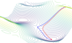
(b)

(c)

(d)

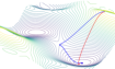
(e)

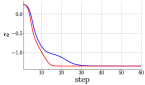
(f)

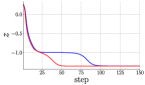
(g)

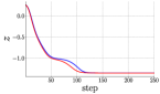
(h)

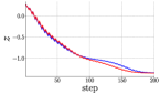
(i)

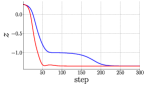
(j)

Figure 4: Illustrations of the effect of GAL (red path/curves) on convergence with various optimizers, in comparison with the standard process (blue path/curves). The top row are convergence paths, while the bottom are the corresponding loss curves. The problem is publicly available in [50].

IV-C Theoretical Properties

This section presents the learning guarantee and remainder error bound for the GAL problem. For simplicity, we denote $h(z;\theta)$ as $h(z)$. Let $v^{*}\in\mathbb{R}^{d}$ be the target adjustment so $z-\tilde{\eta}(\nabla f(z)+v^{*})=z^{*}$. As the gradient adjustment vector is usually small, we assume there exist $a,b\in\mathbb{R}$ so that $v,v^{*}\in[a,b]^{d}\subseteq\mathbb{R}^{d}$, and $z$ is drawn i.i.d. according to the unknown distribution $\mathcal{D}$ and $v^{*}=h^{*}(z)$ where $h^{*}(\cdot)$ is the target labeling function. Moreover, we follow the problem setting in [59] to restrict the loss function to be the $\ell_{p}$ loss ($p\geq 1$) for generalization bound. GAL can be considered as a variant of regression problem that finds the hypothesis $h:\mathbb{R}^{m}\rightarrow[a,b]^{d}$ in a set $\mathcal{H}$ with small generalization error w.r.t. $h^{*}$, i.e.

$$R_{\mathcal{D}}(h)=E_{z\sim\mathcal{D}}\big{[}\ell_{p}(h(z),h^{*}(z))\big{]}.$$

In practice, as $\mathcal{D}$ is unknown, we use the empirical error for approximation over samples in dataset $D$, i.e.

$$\hat{R}_{D}(h)=\frac{1}{|D|}\sum_{i=1}^{|D|}\ell_{p}\big{(}h(z_{i}),v^{*}_{i}\big{)},$$

Theorem IV.1 (Generalization Bound of GAL).

Denote $\mathcal{H}$ as a finite hypothesis set. Given $v,v^{*}\in[a,b]^{d}$, for any $\delta>0$, with probability at least $1-\delta$, the following inequality holds for all $h\in\mathcal{H}$:

$$|R_{\mathcal{D}}(h)-\hat{R}_{D}(h)|\leq\sqrt[p]{d(b-a)^{p}}\cdot\sqrt{\frac{\log|\mathcal{H}|+\log\frac{2}{\delta}}{2|D|}}$$

Proof.

The proof sketch is similar to the classification generalization bound provided in [59]. First, as $\ell_{p}(v,v^{*})=(\sum_{i}^{d}|v_{i}-v^{*}_{i}|^{p})^{\frac{1}{p}}\leq(d(b-a)^{p})^{\frac{1}{p}}$, we know $\ell_{p}$ is bounded by $(d(b-a)^{p})^{\frac{1}{p}}$. Then, by the union bound, given an error $\xi$, we have

$$Pr[\sup_{h\in\mathcal{H}}|R(h)-\hat{R}(h)|>\xi]\leq\sum_{h\in\mathcal{H}}Pr[|R(h)-\hat{R}(h)|>\xi].$$

By Hoeffding’s bound, we have

$$\sum_{h\in\mathcal{H}}Pr[|R(h)-\hat{R}(h)|>\xi]\leq 2|\mathcal{H}|\exp\left(-\frac{2|D|\xi^{2}}{(d(b-a)^{p})^{\frac{2}{p}}}\right).$$

Due to the probability definition, $2|\mathcal{H}|\exp(-\frac{2|D|\xi^{2}}{(d(b-a)^{p})^{\frac{2}{p}}})=\delta$. Considering $\xi$ is a function of other variables, we can rearrange it as $\xi=(d(b-a)^{p})^{\frac{1}{p}}\sqrt{\frac{\log|\mathcal{H}|+\log\frac{2}{\delta}}{2|D|}}$. Since we know $Pr[|R(f)-\hat{R}(f)|>\xi]$ is with probability at most $\delta$, it can be inferred that $Pr[|R(f)-\hat{R}(f)|<=\xi]$ is at least $1-\delta$. It completes the proof. ∎

Remark IV.2.

Theorem IV.1 supports the general intuition that more training data should produce better generalization, which is aligned with conventional learning problems, e.g. classification and regression [59]. Furthermore, distinct from conventional learning problems, the range of gradient adjustments and the dimension could affect the generalization bound.

Theorem IV.3 (Conventional Remainder Error Bound [60]).

Let $f\in C^{1,1}_{L}(\mathbb{R}^{n})$ (i.e. $f$ is once continuously differentiable on $\mathbb{R}^{n}$ and its first-order partial derivative is Lipschitz continuous with constant $L$). Then for any $z^{+},\ z\in\mathbb{R}^{n}$ we have

$$|f(z^{+})-f(z)-\nabla^{\top}f(z)(z^{+}-z)|\leq\frac{L}{2}\|z^{+}-z\|^{2}$$

Theorem IV.4 (Revisited Remainder Error Bound).

Let $f\in C^{1,1}_{L}(\mathbb{R}^{n})$. Given $\tau\in[0,1]$ and any $z^{+},\ z\in\mathbb{R}^{n}$, we denote the minimal angle between vectors $\nabla f(z+\tau(z^{+}-z))-\nabla f(z)$ and $z^{+}-z$ as $\gamma$ and assume the two vectors are non-zero. Then we have

$$|f(z^{+})-f(z)-\nabla^{\top}f(z)(z^{+}-z)|\leq\frac{L}{2}|\cos{\gamma}|\cdot\|z^{+}-z\|^{2}$$

Proof.

Similar to the proof of Theorem IV.3 [60], we use the integral form of the remainder in Taylor’s expansion

$$\ |f(z^{+})-f(z)-\nabla^{\top}f(z)(z^{+}-z)|$$

$$=|\int_{0}^{1}(\nabla f(z+\tau(z^{+}-z))-\nabla f(z))^{\top}(z^{+}-z)d\tau|$$

$$\leq\int_{0}^{1}|(\nabla f(z+\tau(z^{+}-z))-\nabla f(z))^{\top}(z^{+}-z)|d\tau$$

$$=\int_{0}^{1}|\cos{\gamma}|\cdot\|\nabla f(z+\tau(z^{+}-z))-\nabla f(z)\|\cdot\|z^{+}-z\||d\tau$$

$$\leq|\cos{\gamma}|\int_{0}^{1}\|\nabla f(z+\tau(z^{+}-z))-\nabla f(z)\|\cdot\|z^{+}-z\|d\tau$$

$$\leq L\cdot|\cos{\gamma}|\cdot\|z^{+}-z\|^{2}\int_{0}^{1}\tau d\tau$$

$$=\frac{L}{2}|\cos{\gamma}|\cdot\|z^{+}-z\|^{2}$$

It completes the proof. ∎

Remark IV.5.

Theorem IV.4 shows a tighter error bound of the remainder than the well-known bound in Theorem IV.3 [60]. It justifies why properly adjusting gradients direction leads to an effective descent. This is a new insight, as compared to Theorem IV.3. Moreover, it indicates the optimal condition from a geometric perspective, that is, if $z^{+}-z$ is perpendicular to $\nabla f(z+\tau(z^{+}-z))-\nabla f(z)$, the remainder error bound is zero. This is feasible as $z^{+}-z$ is liable to be small in terms of magnitude and $\nabla f(z+\tau(z^{+}-z))-\nabla f(z)$ will not vary dramatically with $\tau\in[0,1]$. In addition, the theorem provides some guideline to design Eq. 4, which forces the adjustment module to find a direction instead of a vector itself for stability.

IV-D Adaptivity to Optimization Methods

To illustrate the effectiveness of the proposed GAL on the optimization process, we employ the 3D problem used in [50], i.e. $z=f(x,y)$, where $x,y,z\in\mathbb{R}$, to visualize the convergence path w.r.t. various optimizers. Fig. 4 show the convergence paths (i.e. top row) and the corresponding curves of $z$ against steps (i.e. bottom row). Specifically, the blue paths/curves are produced by the standard process, while the red ones are produced by the proposed GAL. Given the same starting point, the convergence is affected by the problem and optimizers. The proposed GAL observes the completed convergence steps to learn to adjust the gradients. The resulting convergence curves show that it finds shortcuts to reach the local minimum efficiently. Furthermore, Fig. 4 verifies that the proposed GAL is general in nature and can work with various optimizers.

V Experiments

We comprehensively evaluate the proposed GAL with various models and optimizers. Specifically, we conduct experiment on the image classification task [24, 29], the object detection task [61], and the regression task [18, 19, 20].

V-A Datasets

Following the experimental protocol in [24, 29], we use CIFAR-10/100 [17] and ImageNet [11] for evaluation on the image classification task. Specifically, CIFAR-10 (CIFAR-100) consists of 50,000 32$\times$32 images with 10 (100) classes, while ImageNet has 1000 visual concepts (i.e. classes) and provides average 1000 real-world images on each class. For object detection experiments, we follow the experimental protocol in [61] to use COCO 2017 [12] for evaluation. MS COCO is a large-scale object detection benchmark dataset that consists of 82,783 training images and 40,504 validation images with 80 object categories. Moreover, three datasets, i.e. Boston housing [18], diabetes [19], and California housing [20], are used for the regression task. Specifically, Boston housing includes 506 entries and each entry has 14 features, diabetes consists of 442 samples that have 10 features, and California housing has 20640 samples and each sample has 8 features.

TABLE I: Image classification performance on CIFAR-10. The average error and its standard deviation are over three runs. Architecture (100-32-16) is used for GAL and the number of parameters of GAL is 5K.

Model (optimizer) Error (%) PreResNet-110 (Lookahead) [29] 4.73 DenseNet-121 (Adabound) [24] 5.00 EfficientNet B0 (-) [8] 1.90 EfficientNet B1 (SGD) [50] 1.91 EffcientNet B1 (SGD) reproduced 1.92$\pm$0.12 EffcientNet B1 (SGD) GAL 1.84$\pm$0.06 EffcientNet B1 (Lookahead) reproduced 2.01$\pm$0.02 EffcientNet B1 (Lookahead) GAL 1.91$\pm$0.02 EffcientNet B1 (Adabound) reproduced 3.15$\pm$0.03 EffcientNet B1 (Adabound) GAL 3.03$\pm$0.01

V-B Models & Training Scheme

In the image classification task, we adopt the state-of-the-art EfficientNet [8] on CIFAR, and ResNet [6] and EfficientNet on ImageNet. Originally, EfficientNet is trained on Cloud TPU for 350 epochs with batch size of 2048 [8]. Due to the limitation of computation resources, we follow the training scheme in [50] to train EfficientNet models on CIFAR. Similarly, we employ a publicly available implementation to train ResNet and EfficientNet on ImageNet with 8 NVIDIA V100 GPUs with batch size of 320. We train the models for 90 epochs [6, 29] to provide comparable results. In the object detection task, DEtection TRansformer (DETR) is originally trained with 16 NVIDIA V100 GPUs for 500 epochs [61]. Due to the limitation of computation resources, we follow DETR’s suggestion to train the model with 4 NVIDIA 2080 Ti GPUs for 150 epochs. We use the same hyperparameters as in [61]. Regarding the optimization methods, the model is trained on CIFAR with SGD, Lookahead [29], and Adabound [24]. Following [29], Lookahead is wrapped around SGD in the experiments. The models are trained with RMSProp [21] on ImageNet. DETR is trained with AdamW [62] on MS COCO. The regression experiments run on CPUs with Adam [22].

TABLE II: Image classification performance on CIFAR-100. The average error and its standard deviation are over three runs. Architecture (256-64-32) is used for GAL and the number of parameters of GAL is 47K.

Model (optimizer) Error (%) PreResNet-110 (Lookahead) [29] 21.63 DenseNet-121 (Adabound) [24] - EfficientNet B0 (-) [8] 11.90 EfficientNet B1 (SGD) [50] 11.81 EffcientNet B1 (SGD) reproduced 11.81$\pm$0.10 EffcientNet B1 (SGD) GAL 11.37$\pm$0.10 EffcientNet B1 (Lookahead) reproduced 11.70$\pm$0.01 EffcientNet B1 (Lookahead) GAL 11.44$\pm$0.02 EffcientNet B1 (Adabound) reproduced 14.44$\pm$0.06 EffcientNet B1 (Adabound) GAL 14.12$\pm$0.06

TABLE III: Image classification performance on ImageNet. The average accuracy and its standard deviation are over three runs. Arch (512-128) and (512-256) are used for GAL with ResNet and EfficientNet, respectively. We use 90 epochs in model training for a fair comparison [6, 29].

Model (optimizer) # of parameters Top-1 Top-5 ResNet-50 (SGD) [6]   23M 76.15 92.87 ResNet-50 (Lookahead) [29]   23M 75.49 92.53 EfficientNet-B2 (RMSProp) 350 epochs [8]   9.2M 80.30 95.00 ResNet-50 (RMSProp) reproduced 23.5M 76.43$\pm$0.02 93.05$\pm$0.04 ResNet-50 (RMSProp) GAL 23.5M + 0.70M 76.53$\pm$0.03 93.13$\pm$0.05 EfficientNet-B2 (RMSProp) reproduced   9.2M 77.93$\pm$0.09 93.92$\pm$0.03 EfficientNet-B2 (RMSProp) GAL   9.2M + 0.90M 78.10$\pm$0.06 93.94$\pm$0.06

For the proposed GAL, we employ the MLP, which is simpler than CNN and RNN, throughout this work. GAL takes the feature $z\in\mathbb{R}^{d}$ as input and yields the same dimension output for gradient adjustment. For simplicity, we denote a (N+1)-layer MLP as ($\#_{1}\!-\!\#_{2}\!-\cdots-\!\#_{N}$). For example, (100-32-16) indicates that the architecture consists of four linear transformations that have affine matrices in $\mathbb{R}^{10}\times\mathbb{R}^{100}$, $\mathbb{R}^{100}\times\mathbb{R}^{32}$, $\mathbb{R}^{32}\times\mathbb{R}^{16}$, and $\mathbb{R}^{16}\times\mathbb{R}^{10}$. We use architectures (100-32-16) on CIFAR-10, (256-64-32) on CIFAR-100, and (512-128/256) on ImageNet. Regarding $(\alpha,\beta)$, we use (0.001, 1), (0.01, 1), and (0.01, 10) with SGD, Lookahead, and Adabound, respectively, on CIFAR-10; (0.01, 1), (0.001, 5), and (0.01, 10) with SGD, Lookahead, and Adabound, respectively, on CIFAR-100; and (0.001, 0.001) on ImageNet, respectively. For the object detection tasks, we minimize the remainder w.r.t. predicted bounding box features, i.e. four floats indicating a box. Correspondingly, we use (64-16), 0.01 and 1 as the arch, $\alpha$ and $\beta$, respectively. For the regression task, the architectures of the regression models are (100-50), (64-32), and (256-64) on Boston housing, diabetes, and California housing, respectively. The architectures of the proposed gradient adjustment modules are (16-4), (128-4), and (128-2) on Boston housing, diabetes, and California housing, respectively. We fix $\alpha=0.001$ and $\beta=0.001$ on all three datasets.

TABLE IV: Object detection performance on MS COCO validation with Faster R-CNN. We follow DETR’s suggestion to use 150 epochs in model training [61]. This setting takes approximate 9 days for training DETR-ResNet-50 on a 4-GPU server.

Model Epochs # of parameters AP AP₅₀ AP₇₅ AP_S AP_M AP_L DETR-ResNet-50 [61] 500 41M 42.00 62.40 44.20 20.50 45.80 61.10 DETR-ResNet-101 500 60M 43.50 63.80 46.40 21.90 48.00 61.80 DETR-ResNet-50 reproduced 150 41M 39.13 60.03 40.94 18.30 42.51 58.62 DETR-ResNet-50 GAL 150 41M+1344 39.61 60.55 41.62 18.42 42.52 59.02 DETR-ResNet-101 reproduced 150 60M 40.98 61.91 43.59 19.32 45.09 60.25 DETR-ResNet-101 GAL 150 60M+1344 41.38 62.24 43.87 20.13 45.10 60.86

TABLE V: Regression performance on the Boston housing [18], diabetes [19], and California housing [20] dataset. $\uparrow$ (resp. $\downarrow$) indicates that a larger (resp. smaller) score suggests better performance. The experiments are run 5 times with different random seeds. We also include the analysis of two-sample t-test on the performance of the baseline and the performance of the proposed method to measure the improvement. $t_{stat}$ and $p$ are t-statistics and p value of the t-test, respectively.

Dataset Method Mean Absolute Error (MAE)$\downarrow$ Mean Squared Error (MSE)$\downarrow$ Coefficient of Determination ($R^{2})\uparrow$ Boston housing Baseline 3.9535$\pm$0.4307 23.0956$\pm$4.1695 0.7668$\pm$0.0420 Proposed 2.8079$\pm$0.2720 12.8808$\pm$2.0446 0.8699$\pm$0.0206 $(t_{stat},p)$ (5.02, 1.02e-03) (4.91, 1.17e-03) (-4.92, 1.16e-03) Diabetes Baseline 44.3832$\pm$0.7752 3226.0238$\pm$38.8293 0.3821$\pm$0.0074 Proposed 41.6186$\pm$0.2989 2961.5520$\pm$29.4521 0.4327$\pm$0.0056 $(t_{stat},p)$ (7.43, 7.34e-05) (12.13, 1.97e-06) (-12.14, 1.95e-06) California housing Baseline 1.0910$\pm$0.1297 2.1168$\pm$0.3629 -0.6084$\pm$0.2757 Proposed 0.7780$\pm$0.0262 1.1635$\pm$0.0655 0.1158$\pm$0.0498 $(t_{stat},p)$ (5.28, 7.43e-04) (5.77, 4.15e-04) (-5.78, 4.14e-04)

V-C Performance

Experimental results on CIFAR-10/100, ImageNet, and MS COCO are reported in I, II, Table III, and IV, respectively. As shown in Table I and II, the proposed GAL is able to work with various optimization methods, i.e. SGD, Lookahead, and Adabound, to improve the performance. Also, Table III shows that it is able to work with different models and provides a performance gain. The consistent improvement in object detection can be observed in Table IV on MS COCO. Overall, the proposed GAL improves the convergence of the training process to achieve better accuracies than the standard process with various models on both tasks, which is aligned with the implication of Theorem IV.4. To further evaluate the proposed method, we apply it to the regression task. Specifically, the proposed method is applied on three regression datasets, i.e. Boston housing [18], diabetes [19], and California housing [20]. Three widely-used metrics, i.e. mean absolute error (MAE), mean squared error (MSE), and coefficient of determination ($R^{2}$), are used to evaluate the performance. $R^{2}$ measures the accuracy and efficiency of a model on the data and is a popular metric for regression. A larger $R^{2}$ score indicates better performance in the regression task, while smaller MAE or MSE scores indicate better performance. Experimental results are reported in Table V. The proposed method improves the performance on all three metrics. To further understand the statistical significance of efficacy of the proposed method, we perform a two-sample t-test on the results of the baseline and the ones of the proposed method. According to the $p$ values, the results yielded by the proposed method are statistically significantly from the ones yielded by the baseline with a significance level lower than 0.05.

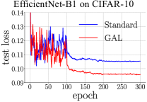
(a)

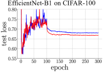
(b)

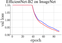
(c)

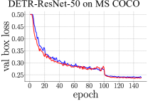
(d)

Figure 5: Validation/test loss curves on various datasets.

VI Analysis

VI-A Generalization Ability and Approximation Remainder

To check the generalization ability of the models trained with GAL, we plot the loss curves on all validation (or test) set in Fig. 5. The losses of the models learned with adjusted gradients are lower than that of the models using vanilla gradients. This implies that the adjusted gradients are better than the vanilla gradients in terms of the generalizability.

Fig. 6 shows the corresponding remainder computed by Eq. (7) and the cosine similarities between vanilla gradients and adjustment vectors on ImageNet. Positive similarities implies that the direction of adjustment vectors has overall smaller angle with vanilla gradient (i.e. smaller than 90^∘). Overall, the proposed adjusted gradients converge to the local minimum more efficiently than the vanilla gradients on all datasets. Note that there is a warm-up in ImageNet training which cause a series of fluctuations at the early epochs, but it stabalizes after 20th epoch.

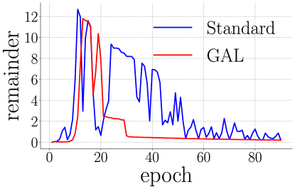
(a)

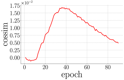
(b)

Figure 6: Remainder curve (left) and cosine similarity curve (right) on ImageNet with EfficientNet-B2.

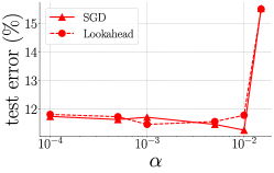
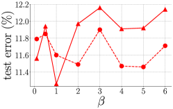
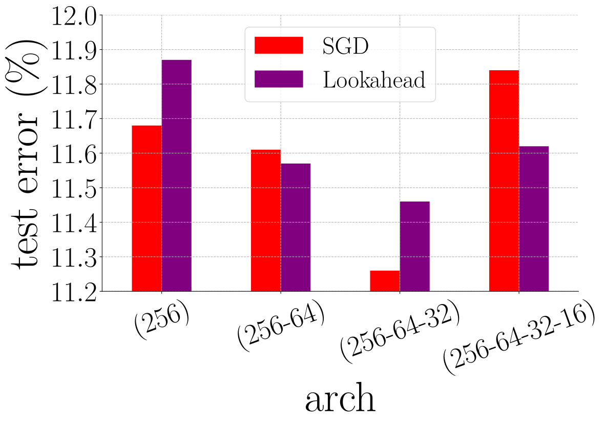
Figure 7: Effects of $\alpha$ (left), $\beta$ (middle), and architecture (right) on CIFAR-100. When varying with $\alpha$, $\beta=1$ (resp. $\beta=5$) with SGD (resp. Lookahead). When varying with $\beta$, $\alpha=0.01$ (resp. $\alpha=0.001$) with SGD (resp. Lookahead). When using different architectures, (i.e. (256), (256-64), (256-64-32), and (256-64-32-16)), $\alpha=0.01$ and $\beta=1$ (resp. $\alpha=0.001$ and $\beta=5$) with SGD (resp. Lookahead).

VI-B Effects of Random Noise

Table VI shows the effect of random noise in the training of EfficientNet on CIFAR-100. The random noise are generated by a uniform or normal distribution to replace the proposed adjustment by Eq. (3). Note that $\alpha\Big{|}\frac{\partial\ell}{\partial z}\Big{|}v/|v|$ is part of the proposed learning approach (see Eq. (4)). The results shows that normalizing the adjustment vector to an appropriate range is definitely required. This is because the gradient is subtle and sophisticated and a large adjustment vector could lead to a divergence in training. Moreover, properly injecting some random noise using the proposed approach (see Eq. (4) and (5)) improves the performance. Yet, the noise is still less effective than the adjustment vector generated by GAL.

VI-C Training Time

To understand the computation overhead, we report the training time of using the baseline and the proposed method in Table VII. In the ImageNet experiment, the learning process without the proposed GAL takes 0.3907 seconds per image to train the model, and takes 0.4027 seconds per image with the proposed GAL. The extra time (i.e. 12 milliseconds) w.r.t. the proposed method is used for the forward and backward process. Similarly, the proposed method take extra 15 (11) milliseconds for training on CIFAR-10 (CIFAR-100). Note that the experiments on CIFAR-10 and CIFAR-100 are run on a workstation equipped with 4 NVIDIA 2080 Ti GPUs, while the experiments on ImageNet are run on a workstation equipped with 8 NVIDIA V100 GPUs.

TABLE VI: Effects of random noise generated by a uniform or normal distribution on the training of EfficientNet with SGD on CIFAR-100. The error rate of the standard learning process is 11.81% while that of GAL is 11.37%.

$v$ $\tilde{v}$ error (%) $\mathcal{U}(-1,1)$ $\alpha\Big{|}\frac{\partial\ell}{\partial z}\Big{|}v/|v|$   (Eq. (4)) 11.62 $\mathcal{U}(-1,1)$ $\alpha\,v/|v|$ 97.20 $\mathcal{N}(0,1)$ $\alpha\Big{|}\frac{\partial\ell}{\partial z}\Big{|}v/|v|$   (Eq. (4)) 11.65 $\mathcal{N}(0,1)$ $\alpha\,v/|v|$ 98.36

TABLE VII: Training time of using the proposed method on each image, in comparison to the one of using the baseline. Note that the proposed gradient adjustment only takes place at the training phase. In other words, the test time w.r.t. the model trained with the proposed method should be identical to the one w.r.t. the model trained with the baseline method.

Dataset Method Time (s) ImageNet Baseline 0.3907 Proposed 0.4027 CIFAR-10 Baseline 0.5292 Proposed 0.5444 CIFAR-100 Baseline 0.5355 Proposed 0.5465

VI-D Effects of Hyperparameters

We analyse the effects of $\alpha$, $\beta$ and various GAL architectures with SGD and Lookahead on CIFAR-100. The performance is shown in Fig. 7. The proposed GAL uses hyperparameters $\alpha=0.01$, $\beta=1$, and architecture = (256-64-32) with SGD, and $\alpha=0.001$, $\beta=5$, and architecture = (256-64-32) with Lookahead. We vary one hyperparameter at a time while the other hyperparameters are kept unchanged in each plot. As shown in the figure, the range $[0.0001,0.01]$ of $\alpha$ consistently leads to lower classification errors. In contrast, classification errors are sensitive to $\beta$, which is optimizer-dependent. $\beta=1$ leads to the best performance with SGD, while $\beta=5$ leads to the best performance with Lookahead. Regarding the effects of architectures, We use architectures (256), (256-64), (256-64-32), and (256-64-32-16) with in Fig. 7 (right). The four architectures have 51.2K, 48.3K, 47.2K, and 46.1K parameters, respectively. Overall, (256-64-32) gives rise to lower classification errors than the other architectures with SGD and Lookahead, while corresponding computational overhead is relatively low.

VI-E Effects of Various Update Policies

As introduced in Algorithm 1, line 7-10, if the tentative loss $\ell_{\sigma}(z-\tilde{\eta}g)$ is less than or equal to the loss $\ell_{\sigma}(z)$, we use $g$ to update the gradients w.r.t. the weights according to the chain rule. We denote this case as line 7 ($\leq$). In the standard process, $\frac{\partial\ell}{\partial z}$ is always used to update the gradients w.r.t. the weights and we denote this case as line 10. We discuss two other possible update policies, i.e. always using $g$ and using $g$ if $\ell_{\sigma}(z-\tilde{\eta}g)$ is less than the loss. We denote these two cases as line 8 and line 7 ($<$), respectively. As shown in Fig. 8a, policy line 8 outperforms line 10 but is not optimal as line 7 ($\leq$). This is because as the training process is close to the local minimum, the loss remainder is much smaller and line 10 would be more efficient than line 8. Moreover, line 7 ($\leq$) is slightly better than line 7 ($<$).

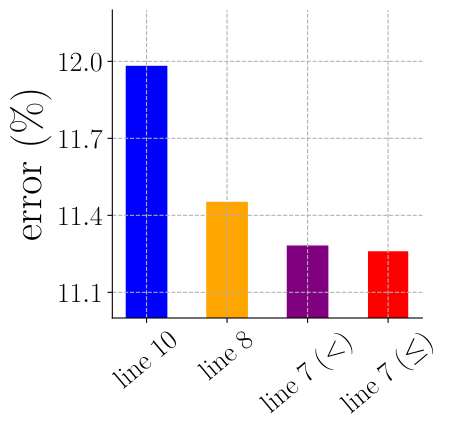
(a) Update policy

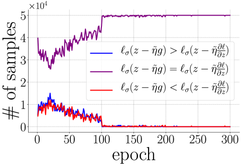
(b) # of improved samples

Figure 8: Ablation study of the proposed GAL with SGD on CIFAR-100. (a) Effects of update policy refers to Algorithm 1 line 7-10. line x means we use line x to generate the update, while line 7 ($<$) means that we modify the if statement in the line 7 as $\ell_{\sigma}(z-\tilde{\eta}g)<\ell_{\sigma}(z)$. (b) Effects of adjusted gradient $g$ and vanilla gradient $\frac{\partial\ell}{\partial z}$ with tentative loss.

VI-F Adjusted Gradient vs. Vanilla Gradient

As the proposed GAL aims to yield adjusted gradient $g$, it would be good to know whether $g$ leads to better descent than $\frac{\partial\ell}{\partial z}$, i.e. lower loss. To do so, we use tentative loss to test $g$ and $\frac{\partial\ell}{\partial z}$. Fig. 8b shows how many times $g$ outperforms $\frac{\partial\ell}{\partial z}$ on samples. The results implies that GAL indeed helps adjust the vanilla gradients with tentative loss on considerable amount of samples in the early stage.

VI-G MLPs vs. CNNs

We explore the effects of using CNNs, instead of MLPs, as the proposed gradient adjustment modules on the classification task. The results of the analysis are reported in Table VIII. It can be seen that CNNs have much larger numbers of parameters than MLPs (except the single layer variant), but achieve lower performance than MLPs. MLPs is a desired choice and their architectures are well aligned with the fact that the discriminative features from modern deep learning models are usually one-dimensional.

TABLE VIII: Effects of MLPs and CNNs with SGD on CIFAR-100. In the case of CNNs, 1-d features (100) would be re-organized to 2-d features (i.e. 10$\times$10), and then multiple convolutional layers with $3\times$3 kernels would be performed on the 2-d features. For example, CNN (256-64) indicates a convolutional layer with 256 3$\times$3 kernels is followed by a convolutional layer with 64 3$\times$3 kernels. Both MLPs and CNNs have a final fully-connected layer, but CNNs have an additional adaptive spatial pooling layer prior to the final layer, which reduces width and height dimensions to 1.

Model Arch Parameters Error (%) MLP (256) 51.2K 11.68 (256-64) 48.3K 11.61 (256-64-32) 47.2K 11.26 (256-64-32-16) 46.1K 11.84 CNN (256) 28.1K 12.15 (256-64) 156.4K 12.13 (256-64-32) 171.7K 11.88 (256-64-32-16) 174.7K 11.75

VII Conclusion

We propose a new learning approach which formulates the remainder as a learning-based problem and leverages the knowledge learned from the past approximations to enhance the learning. To this end, we propose a gradient adjustment learning (GAL) method that employs a model to learn to predict the adjustments on gradients in an end-to-end fashion, which is easy and simple to adapt to the standard training process. Correspondingly, we provide theoretical understanding and experimental results with state-of-the-art models and optimizers in image classification, object detection, and regression tasks. The findings on the experimental results are aligned with the theoretical understanding on the error bound. One intriguing extension of this work is to explore the model design to capture the subtle characteristics of gradient adjustment vectors for the adjustment prediction.

Yan Luo is currently pursuing a Ph.D. degree with the Department of Computer Science and Engineering at the University of Minnesota (UMN), Twin Cities. Prior to UMN, he joined the Sensor-enhanced Social Media (SeSaMe) Centre, Interactive and Digital Media Institute at the National University of Singapore (NUS), as a Research Assistant. Also, he joined the Visual Information Processing Laboratory at the NUS as a Ph.D. Student. He received a B.Sc. degree in computer science from Xi’an University of Science and Technology. He worked in the industry for several years on a distributed system. His research interests include computer vision, computational visual cognition, and deep learning. He is a student member of the IEEE since 2022.

Yongkang Wong is a senior research fellow at the School of Computing, National University of Singapore. He is also the Assistant Director of the NUS Centre for Research in Privacy Technologies (N-CRiPT). He obtained his BEng from the University of Adelaide and PhD from the University of Queensland. He has worked as a graduate researcher at NICTA’s Queensland laboratory, Brisbane, OLD, Australia, from 2008 to 2012. His current research interests are in the areas of Image/Video Processing, Machine Learning, Action Recognition, and Human Centric Analysis. He is a member of the IEEE since 2009.

Mohan S. Kankanhalli is Provost’s Chair Professor of Computer Science at the National University of Singapore (NUS). He is the Dean of NUS School of Computing and he also directs N-CRiPT (NUS Centre for Research in Privacy Technologies) which conducts research on privacy on structured as well as unstructured (multimedia, sensors, IoT) data. Mohan obtained his BTech from IIT Kharagpur and MS & PhD from the Rensselaer Polytechnic Institute. Mohan’s research interests are in Multimedia Computing, Computer Vision, Information Security & Privacy and Image/Video Processing. He has made many contributions in the area of multimedia & vision – image and video understanding, data fusion, visual saliency as well as in multimedia security – content authentication and privacy, multi-camera surveillance. Mohan is a Fellow of IEEE.

Qi Zhao is an associate professor in the Department of Computer Science and Engineering at the University of Minnesota, Twin Cities. Her main research interests include computer vision, machine learning, cognitive neuroscience, and healthcare. She received her Ph.D. in computer engineering from the University of California, Santa Cruz in 2009. She was a postdoctoral researcher in the Computation & Neural Systems at the California Institute of Technology from 2009 to 2011. Before joining the University of Minnesota, Qi was an assistant professor in the Department of Electrical and Computer Engineering and the Department of Ophthalmology at the National University of Singapore. She has published more than 100 journal and conference papers, and edited a book with Springer, titled Computational and Cognitive Neuroscience of Vision, that provides a systematic and comprehensive overview of vision from various perspectives. She serves as an associate editor of IEEE TNNLS and IEEE TMM, as a program chair WACV’22, and as an organizer and/or area chair for CVPR and other major venues in computer vision and AI regularly. She is a member of the IEEE since 2004.

References

- [1] S. Xia, M. Shao, J. Luo, and Y. Fu, “Understanding kin relationships in a photo,” IEEE Trans. Multim., vol. 14, no. 4, pp. 1046–1056, 2012.
- [2] C. Ding and D. Tao, “Robust face recognition via multimodal deep face representation,” IEEE Trans. Multim., vol. 17, no. 11, pp. 2049–2058, 2015.
- [3] Y. Zhan and R. Zhang, “No-reference image sharpness assessment based on maximum gradient and variability of gradients,” IEEE Trans. Multim., vol. 20, no. 7, pp. 1796–1808, 2018.
- [4] S. I. Cho and S. Kang, “Gradient prior-aided CNN denoiser with separable convolution-based optimization of feature dimension,” IEEE Trans. Multim., vol. 21, no. 2, pp. 484–493, 2019.
- [5] B. Xu, J. Li, Y. Wong, Q. Zhao, and M. S. Kankanhalli, “Interact as you intend: Intention-driven human-object interaction detection,” IEEE Trans. Multim., vol. 22, no. 6, pp. 1423–1432, 2020.
- [6] K. He, X. Zhang, S. Ren, and J. Sun, “Deep residual learning for image recognition,” in IEEE Conference on Computer Vision and Pattern Recognition, 2016, pp. 770–778.
- [7] A. Krizhevsky, I. Sutskever, and G. E. Hinton, “ImageNet classification with deep convolutional neural networks,” in Advances in Neural Information Processing Systems, 2012, pp. 1097–1105.
- [8] M. Tan and Q. V. Le, “Efficientnet: Rethinking model scaling for convolutional neural networks,” in International Conference on Machine Learning, ser. Proceedings of Machine Learning Research, K. Chaudhuri and R. Salakhutdinov, Eds., vol. 97. PMLR, 2019, pp. 6105–6114.
- [9] K. He, G. Gkioxari, P. Dollár, and R. Girshick, “Mask R-CNN,” in IEEE International Conference on Computer Vision, 2017, pp. 2961–2969.
- [10] S. Ren, K. He, R. Girshick, and J. Sun, “Faster R-CNN: Towards real-time object detection with region proposal networks,” in Advances in Neural Information Processing Systems, 2015, pp. 91–99.
- [11] J. Deng, W. Dong, R. Socher, L.-J. Li, K. Li, and L. Fei-Fei, “ImageNet: A large-scale hierarchical image database,” in IEEE Conference on Computer Vision and Pattern Recognition, 2009, pp. 248–255.
- [12] T.-Y. Lin, M. Maire, S. Belongie, J. Hays, P. Perona, D. Ramanan, P. Dollár, and C. L. Zitnick, “Microsoft COCO: Common objects in context,” in European conference on computer vision, ser. Lecture Notes in Computer Science, vol. 8693, 2014, pp. 740–755.
- [13] S. Boyd, S. P. Boyd, and L. Vandenberghe, Convex optimization. Cambridge University Press, 2004.
- [14] L. Bottou, F. E. Curtis, and J. Nocedal, “Optimization methods for large-scale machine learning,” SIAM Review, vol. 60, no. 2, pp. 223–311, 2018.
- [15] H. Robbins and S. Monro, “A stochastic approximation method,” The Annals of Mathematical Statistics, pp. 400–407, 1951.
- [16] Z. Zhu, J. Wu, B. Yu, L. Wu, and J. Ma, “The anisotropic noise in stochastic gradient descent: Its behavior of escaping from sharp minima and regularization effects.” in International Conference on Machine Learning, 2019, pp. 7654–7663.
- [17] A. Krizhevsky, “Learning multiple layers of features from tiny images,” Master’s thesis, University of Toronto, 2009.
- [18] D. Harrison Jr and D. L. Rubinfeld, “Hedonic housing prices and the demand for clean air,” Journal of environmental economics and management, vol. 5, no. 1, pp. 81–102, 1978.
- [19] D. Dua and C. Graff, “UCI machine learning repository,” 2017.
- [20] R. K. Pace and R. Barry, “Sparse spatial autoregressions,” Statistics & Probability Letters, vol. 33, no. 3, pp. 291–297, 1997.
- [21] G. Hinton, N. Srivastava, and K. Swersky, “Neural networks for machine learning. lecture 6a. overview of mini-batch gradient descent.”
- [22] D. P. Kingma and J. Ba, “Adam: A method for stochastic optimization,” in International Conference on Learning Representations, 2015.
- [23] L. Liu, H. Jiang, P. He, W. Chen, X. Liu, J. Gao, and J. Han, “On the variance of the adaptive learning rate and beyond,” in International Conference on Learning Representations, 2020.
- [24] L. Luo, Y. Xiong, and Y. Liu, “Adaptive gradient methods with dynamic bound of learning rate,” in International Conference on Learning Representations, 2019.
- [25] J. Zhuang, T. Tang, Y. Ding, S. C. Tatikonda, N. Dvornek, X. Papademetris, and J. Duncan, “AdaBelief Optimizer: Adapting Stepsizes by the Belief in Observed Gradients,” Advances in Neural Information Processing Systems, vol. 33, 2020.
- [26] Y. Carmon, J. C. Duchi, O. Hinder, and A. Sidford, “Accelerated methods for nonconvex optimization,” SIAM Journal on Optimization, vol. 28, no. 2, pp. 1751–1772, 2018.
- [27] C. Jin, R. Ge, P. Netrapalli, S. M. Kakade, and M. I. Jordan, “How to escape saddle points efficiently,” in International Conference on Machine Learning, 2017, pp. 1724–1732.
- [28] S. Reddi, M. Zaheer, S. Sra, B. Poczos, F. Bach, R. Salakhutdinov, and A. Smola, “A generic approach for escaping saddle points,” in International Conference on Artificial Intelligence and Statistics, 2018, pp. 1233–1242.
- [29] M. Zhang, J. Lucas, J. Ba, and G. E. Hinton, “Lookahead optimizer: k steps forward, 1 step back,” in Advances in Neural Information Processing Systems, 2019, pp. 9593–9604.
- [30] M. Andrychowicz, M. Denil, S. Gomez, M. W. Hoffman, D. Pfau, T. Schaul, B. Shillingford, and N. De Freitas, “Learning to learn by gradient descent by gradient descent,” in Advances in Neural Information Processing Systems, 2016, pp. 3981–3989.
- [31] Y. Chen, M. W. Hoffman, S. G. Colmenarejo, M. Denil, T. P. Lillicrap, M. Botvinick, and N. Freitas, “Learning to learn without gradient descent by gradient descent,” in International Conference on Machine Learning, 2017, pp. 748–756.
- [32] J. Ji, X. Chen, Q. Wang, L. Yu, and P. Li, “Learning to learn gradient aggregation by gradient descent.” in International Joint Conferences on Artificial Intelligence, 2019, pp. 2614–2620.
- [33] D. E. Rumelhart, G. E. Hinton, and R. J. Williams, “Learning representations by back-propagating errors,” Nature, vol. 323, no. 6088, pp. 533–536, 1986.
- [34] M. Tan and Q. V. Le, “EfficientNetV2: Smaller models and faster training,” in International Conference on Machine Learning, ser. Proceedings of Machine Learning Research, M. Meila and T. Zhang, Eds., vol. 139. PMLR, 2021, pp. 10 096–10 106.
- [35] A. Dosovitskiy, L. Beyer, A. Kolesnikov, D. Weissenborn, X. Zhai, T. Unterthiner, M. Dehghani, M. Minderer, G. Heigold, S. Gelly, J. Uszkoreit, and N. Houlsby, “An image is worth 16x16 words: Transformers for image recognition at scale,” in International Conference on Learning Representations, 2021.
- [36] I. O. Tolstikhin, N. Houlsby, A. Kolesnikov, L. Beyer, X. Zhai, T. Unterthiner, J. Yung, A. Steiner, D. Keysers, J. Uszkoreit, M. Lucic, and A. Dosovitskiy, “Mlp-mixer: An all-mlp architecture for vision,” CoRR, vol. abs/2105.01601, 2021.
- [37] Y. Cong, J. Yuan, and J. Luo, “Towards scalable summarization of consumer videos via sparse dictionary selection,” IEEE Trans. Multim., vol. 14, no. 1, pp. 66–75, 2012.
- [38] K. Yadati, H. Katti, and M. S. Kankanhalli, “CAVVA: computational affective video-in-video advertising,” IEEE Trans. Multim., vol. 16, no. 1, pp. 15–23, 2014.
- [39] S. Bu, Z. Liu, J. Han, J. Wu, and R. Ji, “Learning high-level feature by deep belief networks for 3-d model retrieval and recognition,” IEEE Trans. Multim., vol. 16, no. 8, pp. 2154–2167, 2014.
- [40] L. Zhang, Y. Gao, Y. Xia, K. Lu, J. Shen, and R. Ji, “Representative discovery of structure cues for weakly-supervised image segmentation,” IEEE Trans. Multim., vol. 16, no. 2, pp. 470–479, 2014.
- [41] K. Cho, A. C. Courville, and Y. Bengio, “Describing multimedia content using attention-based encoder-decoder networks,” IEEE Trans. Multim., vol. 17, no. 11, pp. 1875–1886, 2015.
- [42] C. Zhang, J. Cheng, and Q. Tian, “Unsupervised and semi-supervised image classification with weak semantic consistency,” IEEE Trans. Multim., vol. 21, no. 10, pp. 2482–2491, 2019.
- [43] J. Li, Y. Wong, Q. Zhao, and M. S. Kankanhalli, “Visual social relationship recognition,” Int. J. Comput. Vis., vol. 128, no. 6, pp. 1750–1764, 2020.
- [44] J. Li, Z. Xu, Y. Wong, Q. Zhao, and M. Kankanhalli, “GradMix: Multi-source transfer across domains and tasks,” in IEEE Winter Conference on Applications of Computer Vision, 2020, pp. 3019–3027.
- [45] Y. Luo, Y. Wong, M. S. Kankanhalli, and Q. Zhao, “n-reference transfer learning for saliency prediction,” in European Conference Computer Vision, ser. Lecture Notes in Computer Science, A. Vedaldi, H. Bischof, T. Brox, and J. Frahm, Eds., vol. 12353. Springer, 2020, pp. 502–519.
- [46] I. J. Goodfellow, J. Shlens, and C. Szegedy, “Explaining and harnessing adversarial examples,” in International Conference on Learning Representations, Y. Bengio and Y. LeCun, Eds., 2015.
- [47] P. Foret, A. Kleiner, H. Mobahi, and B. Neyshabur, “Sharpness-aware minimization for efficiently improving generalization,” in International Conference on Learning Representations, 2021.
- [48] F. Pedregosa, “Hyperparameter optimization with approximate gradient,” in International Conference on Machine Learning, ser. JMLR Workshop and Conference Proceedings, M. Balcan and K. Q. Weinberger, Eds., vol. 48. JMLR.org, 2016, pp. 737–746.
- [49] D. Lopez-Paz and M. Ranzato, “Gradient episodic memory for continual learning,” in Advances in Neural Information Processing Systems, 2017, pp. 6467–6476.
- [50] Y. Luo, Y. Wong, M. Kankanhalli, and Q. Zhao, “Direction concentration learning: Enhancing congruency in machine learning,” IEEE Transactions on Pattern Analysis and Machine Intelligence, pp. 1–1, 2019.
- [51] N. I. Achieser, Theory of approximation. Courier Corporation, 2013.
- [52] A. F. Timan, Theory of approximation of functions of a real variable. Elsevier, 2014.
- [53] M. Berz and G. Hoffstätter, “Computation and application of taylor polynomials with interval remainder bounds,” Reliable Computing, vol. 4, no. 1, pp. 83–97, 1998.
- [54] W. E. Milne, “The remainder in linear methods of approximation,” Journal of Research of the National Bureau of Standards, vol. 43, no. 5, pp. 501–511, November 1949.
- [55] D. D. Stancu, “Evaluation of the remainder term in approximation formulas by Bernstein polynomials,” Mathematics of Computation, vol. 17, no. 83, pp. 270–278, 1963.
- [56] ——, “The remainder of certain linear approximation formulas in two variables,” Journal of the Society for Industrial and Applied Mathematics, Series B: Numerical Analysis, vol. 1, no. 1, pp. 137–163, 1964.
- [57] V. N. Vapnik, “An overview of statistical learning theory,” IEEE Transactions on Neural Networks, vol. 10, no. 5, pp. 988–999, 1999.
- [58] P. E. Black, “Greedy algorithm,” Dictionary of Algorithms and Data Structures, vol. 2, p. 62, 2005.
- [59] M. Mohri, A. Rostamizadeh, and A. Talwalkar, Foundations of Machine Learning. The MIT Press, 2012.
- [60] Y. Nesterov, Introductory Lectures on Convex Optimization: A Basic Course. Springer Science & Business Media, 2013.
- [61] N. Carion, F. Massa, G. Synnaeve, N. Usunier, A. Kirillov, and S. Zagoruyko, “End-to-end object detection with transformers,” in European Conference on Computer Vision, ser. Lecture Notes in Computer Science, vol. 12346, 2020, pp. 213–229.
- [62] I. Loshchilov and F. Hutter, “Decoupled weight decay regularization,” in International Conference on Learning Representations, 2019.