Distributed Learning of Generalized Linear Causal Networks

Abstract

We consider the task of learning causal structures from data stored on multiple machines, and propose a novel structure learning method called distributed annealing on regularized likelihood score (DARLS) to solve this problem. We model causal structures by a directed acyclic graph that is parameterized with generalized linear models, so that our method is applicable to various types of data. To obtain a high-scoring causal graph, DARLS simulates an annealing process to search over the space of topological sorts, where the optimal graphical structure compatible with a sort is found by a distributed optimization method. This distributed optimization relies on multiple rounds of communication between local and central machines to estimate the optimal structure. We establish its convergence to a global optimizer of the overall score that is computed on all data across local machines. To the best of our knowledge, DARLS is the first distributed method for learning causal graphs with such theoretical guarantees. Through extensive simulation studies, DARLS has shown competing performance against existing methods on distributed data, and achieved comparable structure learning accuracy and test-data likelihood with competing methods applied to pooled data across all local machines. In a real-world application for modeling protein-DNA binding networks with distributed ChIP-Sequencing data, DARLS also exhibits higher predictive power than other methods, demonstrating a great advantage in estimating causal networks from distributed data.

Keywords: Causal graphs, distributed learning, generalized linear models, simulated annealing, topological sorts.

1 Introduction

Causal diagrams are mathematical models for cause-effect relationships among variables (Pearl 1995), with applications in education (Dehejia and Wahba 1999; Hill 2012), economics (Imbens 2004), and epidemiology (Glymour 2006), etc. A causal diagram is represented by a directed acyclic graph (DAG), where edges encode causal effects among variables (nodes). Graphical models associated with DAGs are known as Bayesian networks (BNs). The probability density of a set of random variables $\{X_{1},\ldots,X_{p}\}$ in a BN factorizes as

$$p(x_{1},\ldots,x_{p})=\prod_{j=1}^{p}p(x_{j}\mid\text{PA}_{j}=pa_{j}),$$ (1)

where $\text{PA}_{j}\subset\{X_{1},\ldots,X_{p}\}\setminus\{X_{j}\}$ is the parent set of ${X_{j}}$ with $pa_{j}$ being its value. Since randomized experiments are not always feasible, various approaches have been put forward to learn causal DAGs from observational data (Pearl 2009; Guo et al. 2020).

In this work, we focus on learning causal DAGs from distributed data. Distributed data storage has been used for privacy protection when managing the copious amount of data generated everyday by government agencies, research institutions, medical centers, technology companies, etc (Mehmood et al. 2016). Many of these organizations collect similar data, or data from the same population, and they often collaborate in social, scientific and business domains. For example, in 2021, Google and Apple were initiating an exposure notification system that tracks potential exposure to COVID-19 and a privacy-preserving analytics platform that collects health metrics (Apple and Google 2021). Also, small clinics often combine data to obtain statistically significant results since the individual datasets are otherwise too small. Such collaborations always require privacy disclosures stating that each institution cannot share the privately-hold sensitive data with the other parties. Even when data privacy is not a concern, merging data from multiple sources remains a difficult task. Since each local agency stores and manages data with different platforms, it is often time-consuming to extract, standardize and migrate the data. From a purely computational perspective, distributed computing often uses parallelism across local machines, resulting in substantial reduction in computation time and allowing us to scale inference procedures to massive datasets.

The widespread use of distributed data has lead to a research area whose goal is to adapt common statistical and machine learning tasks to the distributed setting. A straightforward idea for deriving a distributed version of any inference procedure is to form a global estimate by averaging the local estimates, an approach known as one-shot parameter averaging. This approach, however, fails to obtain solutions with any desired level of suboptimality compared to the global estimate constructed based on all the data (Zinkevich et al. 2010; Shamir et al. 2014). To overcome drawbacks of one-shot averaging, communication-efficient algorithms have been proposed that utilize multiple rounds of communication between local and central machines to generate a sequence of (global) estimates (Zhang et al. 2013; Shamir et al. 2014; Jordan et al. 2018; Fan et al. 2019). Communication-efficient algorithms are particularly useful in distributed optimization of multi-agent systems, such as electronic power systems, sensor networks and smart manufacturing (Molzahn et al. 2017; Yang et al. 2019).

Despite these methodological advances, learning causal DAGs from data distributed across independent machines is still a challenging task. A major difficulty is how to integrate local information to form a global causal graph that satisfies the acyclicity constraint. One approach is to iterate over local datasets (once) and then combine the local graphs or the local p-values to form a global graph (Na and Yang 2010; Gou et al. 2007; Tang et al. 2019). However, there is no theoretical guarantee that aggregating local estimates, using this single-iteration approach, would lead to an estimate close to the global minimizer of the loss on the combined data. In this paper, we propose a score-based learning method that carries out multiple rounds of communication to estimate DAGs from distributed data. Our objective function is equivalent to a regularized log-likelihood of the overall data. To optimize it, the central machine proposes a candidate ordering $\pi$, where the score of $\pi$ is evaluated via communication with local machines over DAGs compatible with $\pi$. Then, the candidate sort $\pi$ is selected by simulated annealing. Because every DAG has at least one ordering, searching over the space of orderings ensures that the acyclicity constraint is always satisfied. We show that the convergence rate of our distributed estimate to the global one is $O(\log(n)/\sqrt{m})$ for a fixed true DAG, where $n$ is the total sample size across all local machines and $m$ is the smallest local sample size  (Theorem 1, Section 4.1). To the best of our knowledge, our approach is the first to learn causal graphs from distributed data with a theoretical guarantee of convergence to the global estimate as the sample size of the local machines grow.

Another contribution of our work is the use of generalized linear models (GLMs) for local conditional distributions in BNs, which brings several advantages to causal structure learning. Our proposed GLM DAG model is a flexible family for various data types beyond linear Gaussian models (with equal variance) and multi-logit models (Gu et al. 2019; Aragam et al. 2019), and hence it can be applied to multiple domains. Additionally, most models in the GLM family lead to convex loss functions which facilitate the optimization task. The objective function in our distributed learning algorithm is equivalent to a regularized likelihood of the overall data, which has been shown to be effective in learning both continuous and discrete DAGs (Fu and Zhou 2013; Aragam and Zhou 2015; Gu et al. 2019; Ye et al. 2021). Furthermore, we show that GLM DAG models lead to the identifiability of the underlying causal DAGs (Proposition 1, Section 2), while other common models, such as multinomial for discrete networks and Gaussian linear DAGs, are not identifiable in general (Pearl 1995; Heckerman et al. 1995). Under such identifiability, we establish the $\ell_{2}$-consistency of a global maximizer DAG of our regularized likelihood score (Theorem 2, Section 4.2).

The paper is organized as follows. Section 2 defines the generalized linear DAG model and establishes some identifiability results under this model. In Section 3, we set up the optimization problem for learning causal graphs and develop the DARLS algorithm that combines simulated annealing to search over permutation space and a distributed optimization algorithm to optimize the network structure given an ordering. We then establish theoretical results for the convergence of the distributed optimization algorithm and estimation consistency of DARLS in Section 4. Section 5 consists of exhaustive simulation experiments, where we compare our method to existing ones using distributed data, test the robustness of DARLS against violations of its underlying model assumptions, and examine the accuracy loss and computational efficiency of distributed learning. We also apply the distributed learning methods to ChIP-sequencing data for modeling protein-DNA binding networks in Section 6. The paper is concluded with a discussion in Section 7. All proofs are relegated to the supplementary material.

2 Generalized linear DAG models

Denote by $x^{j}\in\mathbb{R}^{d_{j}}$ a realization of variable $X_{j}$, where $d_{j}=1$ for a numerical $X_{j}$ and $d_{j}=r_{j}-1$ for a categorical variable $X_{j}$ with $r_{j}$ classes, using the one-hot encoding. Let $\beta_{ij}\in\mathbb{R}^{d_{i}\times d_{j}}$ encode the influence of $X_{i}$ on $X_{j}$ and $\beta_{ij}=0$ if $X_{i}\notin\text{PA}_{j}$. Put

$$\beta_{j}:=[\beta_{0j},\beta_{1j},\ldots,\beta_{pj}]\in\mathbb{R}^{(d+1)\times d_{j}},\quad x:=[1,x^{1},\ldots,x^{p}]\in\mathbb{R}^{d+1},$$ (2)

where $\beta_{0j}\in\mathbb{R}^{1\times d_{j}}$ and $d=\sum_{i=1}^{p}d_{i}$. Here and elsewhere, $[x,y]$ denotes the vertical concatenation of two vectors or matrices $x$ and $y$. We define a generalized linear DAG (GLDAG) as the Bayesian network (1) with conditional densities given by GLMs with canonical links, that is,

$$p(x^{j}\mid pa_{j},\beta_{j}) =\exp\left(\langle\beta_{j}^{\top}x,x^{j}\rangle-b_{j}(\beta_{j}^{\top}x)\right)+c_{j}(x^{j}),\quad j\in[p]$$ (3)

where $b_{j}$ and $c_{j}$ are both functions from $\mathbb{R}^{d_{j}}$ to $\mathbb{R}$. Note that $\beta_{j}^{\top}x=\sum_{i\in\text{PA}_{j}}\beta_{ij}^{\top}x^{i}$ only depends on $pa_{j}$. GLDAG models allow for many common distributions via the choice of the log partition-function $b_{j}(\cdot)$. Examples include the Bernoulli distribution for $b_{j}(\theta)=\log(1+e^{\theta})$, constant-variance Gaussian for $b_{j}(\theta)=\theta^{2}/2$, Poisson for $b_{j}(\theta)=\exp(\theta)$, Gamma for $b_{j}(\theta)=-\log(-\theta)$ and the multinomial for $b_{j}(\theta)=\log\bigl{(}1+\sum_{l=1}^{d_{j}}e^{\theta_{l}}\bigr{)}$. Note that in the multinomial case $b_{j}(\cdot)$ is a multivariate function, operating on a vector $\theta=(\theta_{l})$, in contrast to the other example for which $b_{j}(\cdot)$ is a scalar function. The Bernoulli and multinomial choices above give rise to logistic and multi-logit regression models for each node.

We collect all the parameters of model (3) in a matrix $\beta\in\mathbb{R}^{(d+1)\times d}$ which is obtained by horizontal concatenation of $\beta_{j},j=1,\dots,p$, each as defined in (2). We say that a GLDAG (3) is continuous if all the variables are continuous. Recall that in this case, $d_{j}=1$ for all $j\in[p]$ and thus $\beta$ is a $(p+1)\times p$ matrix. We rewrite the log pdf of (3), in the continuous case, as

$$L(x;\beta)=\sum_{j=1}^{p}\big{[}\log c_{j}(x^{j})+x^{j}(\beta^{\top}x)_{j}-b_{j}\big{(}(\beta^{\top}x)_{j}\big{)}\big{]},$$ (4)

where $\beta^{\top}x\in\mathbb{R}^{p}$ and $\beta_{ij}\neq 0$ if and only if $X_{i}\to X_{j}$. Next, we define identifiability of DAG models following Peters et al. (2014); Hoyer et al. (2008); Peters and Bühlmann (2014), and show that continuous GLDAGs are identifiable.

Definition 1 (Identifiability).

Suppose we are given a joint distribution $L(X)=L(X_{1},\ldots,X_{p})$ that has been generated from an unknown GLDAG model (3) with a graph $\mathcal{G}_{0}$. If the distribution $L(X)$ cannot be generated by any GLDAG model with a different graph $\mathcal{G}\neq\mathcal{G}_{0}$, then we say $\mathcal{G}_{0}$ is identifiable from $L(X)$.

It is well-known that linear Gaussian DAGs and multinomial DAGs in general are not identifiable (Pearl 1995; Heckerman et al. 1995). In contrast, continuous GLDAG models (4) are identifiable under mild assumptions:

Proposition 1.

Suppose the joint distribution $L(X)$ is defined by the log-pdf $L(x;\beta)$ with a DAG $\mathcal{G}_{0}$ according to (4) such that $\beta_{ij}\neq 0$ if and only if $i\in\text{PA}_{j}$ in $\mathcal{G}_{0}$. If $L(x;\beta)$ is second-order differentiable with respect to $x$ and the first-order derivative of $b_{j}(\cdot)$ exists and is not constant for all $j$, then $\mathcal{G}_{0}$ is identifiable from $L(X)$.

Proposition 1 establishes the identifiability of continuous GLDAG models (4), partially justifying our goal as to learn causal graphs. This result also expands the class of identifiable DAG models in the literature. DAGs generated from linear Gaussian structural equation models with equal variance can be fully identified (Peters and Bühlmann 2014), which is a special case of the GLDAG models with $b_{j}(\theta)=\theta^{2}/2,\leavevmode\nobreak\ \forall j$. A different class of identifiable DAG models is the additive noise model, $X_{j}=f_{j}(\text{PA}_{j})+\varepsilon_{j}$, assuming nonlinear $f_{j}$ and/or non-Gaussian $\varepsilon_{j}$ (Shimizu et al. 2006; Hoyer et al. 2008; Peters et al. 2014).

3 Distributed DAG learning

In this section, we construct the objective function using distributed data and propose a simulated annealing search combined with an iterative optimization method to learn causal DAG structures. We start with the definition of topological sorts for DAGs. Given a permutation $\pi$ on $[p]:=\{1,\ldots,p\}$, we permute a vector $v=(v_{1},\ldots,v_{p})$ according to $\pi$ to obtain a relabeled vector $v_{\pi}=\left(v_{\pi(1)},\ldots,v_{\pi(p)}\right)$. A topological sort of a DAG is a permutation of nodes such that if $a\in\text{PA}_{b}$, then $a$ precedes $b$ in the order defined by $\pi$, denoted by $a\prec_{\pi}b$. By definition (1), every DAG has at least one topological sort.

Let $\{x_{h}\}_{h=1}^{n}$ be an i.i.d. sample of size $n$ from model (3). We also let $x_{h}^{j}$ represent the observed value of the $j$-th variable ($X_{j}$) in the $h$-th data point. Consider a subset $\mathcal{I}\subset[n]$. The normalized negative log-likelihood of the subsample $\{x_{h}\}_{h\in\mathcal{I}}$ is given, up to an additive constant, by

$$\ell_{\mathcal{I}}(\beta):=\frac{1}{|\mathcal{I}|}\sum_{h\in\mathcal{I}}\sum_{j=1}^{p}\bigl{[}b_{j}(\beta_{j}^{\top}x_{h})-\langle\beta_{j}^{\top}x_{h},x_{h}^{j}\rangle\bigr{]}.$$ (5)

Note that in this notation, $\ell_{[n]}$ denotes the normalized negative log-likelihood of the entire sample of size $n$.

3.1 Global objective function and annealing

We consider the case that the overall data is stored on $K$ different servers, where each local machine $\mathcal{M}_{k}$ holds its private data $\{x_{h}\}_{h\in\mathcal{I}_{k}}$ and communicates with a central machine $\mathcal{C}$. Let $n_{k}=|\mathcal{I}_{k}|$ be the sample size in $\mathcal{M}_{k}$ so that $\sum_{k=1}^{K}n_{k}=n$. The normalized negative log-likelihood based on the entire data can be decomposed as $\ell_{[n]}(\beta)=\sum_{k=1}^{K}\frac{n_{k}}{n}\ell_{\mathcal{I}_{k}}(\beta)$. Let $\mathcal{P}$ be the set of all permutations on $[p]$ and $\mathcal{D}(\pi)\subset\mathbb{R}^{(d+1)\times d}$ the set of DAGs whose topological sorts are compatible with a permutation $\pi\in\mathcal{P}$. Note that $\mathcal{D}(\pi)$ is a linear subspace of $\mathbb{R}^{(d+1)\times d}$. We ideally would like to estimate $\beta$ by minimizing a regularized loss function of the form

$$\min_{\pi\in\mathcal{P}}f(\pi),\quad\text{where}\quad f(\pi):=\min_{\beta\in\mathcal{D}(\pi)}\sum_{k=1}^{K}\frac{n_{k}}{n}\ell_{\mathcal{I}_{k}}(\beta)+\rho(\beta),$$ (6)

and $\rho(\cdot)$ is an appropriate regularizer to promote sparsity in $\beta$. We call $f(\pi)$ the global objective function since it is defined using all data across local machines.

Recall that $\beta_{ij}\neq 0$ if and only if $i\in\text{PA}_{j}$. To learn sparse DAGs, we apply group regularization of the form

$$\rho(\beta)=\lambda\sum_{i,j}\rho_{g}(\beta_{ij}),$$ (7)

where $\rho_{g}(\cdot)$ is a nonnegative and nondecreasing group regularizer and $\lambda>0$ is a tuning parameter. Restricted to $\mathcal{D}(\pi)$, the regularizer can be further simplfied to $\rho(\beta)=\lambda\sum_{j}\sum_{i\prec_{\pi}j}\rho_{g}\left(\beta_{ij}\right)$. In this paper, we consider the Group Lasso (i.e., group $\ell_{2}$) penalty with the choice

$$\rho_{g}(\beta_{ij})=|\!|\!|\beta_{ij}|\!|\!|_{F},$$ (8)

where $|\!|\!|\beta_{ij}|\!|\!|_{F}$ is the Frobenius norm of matrix $\beta_{ij}$. As a convex penalty and a natural extension of Lasso regularization, Group Lasso has demonstrated remarkable performance in grouped variable selection (Yuan and Lin 2007).

To search over $\left(\pi\in\mathcal{P},\beta\in\mathcal{D}(\pi)\right)$ with distributed data as in (6), we propose the distributed annealing on regularized likelihood score (DARLS) algorithm, which applies annealing strategies to search over the permutation space, coupled with a distributed optimization method. Such manner of joint optimization over the topological sort space and the DAG space has demonstrated great effectiveness in learning BNs; see for example, Larrañaga et al. (1996); Friedman and Koller (2003); Scanagatta et al. (2015); Ye et al. (2021) and the references thereof.

The main steps of DARLS are outlined in Algorithm 1. At each annealing iteration, a permutation $\pi^{*}$ is proposed based on current $\widehat{\pi}$ (line 5) and is accepted with probability according to simulated annealing given a decreasing temperature schedule. To compute the score of the optimal DAG structure for a given permutation, we use the distributed optimization approach outlined in Algorithm 2, the details of which are discussed in Section 3.2 below. This approach allows multiple rounds of communications between local and the central machines to update and synthesize information. Note that DARLS can be applied to any objective function as long as the gradient w.r.t. $\beta$ has a closed-form expression.

Algorithm 1 Distributed annealing on regularized likelihood score (DARLS).

Input: $\{x_{h}\}_{h=1}^{n}$ distributed over $K$ machines, $\pi_{0}$, a temperature schedule $\{T^{(i)}\}_{i=0}^{N}$, $\tau$.
      Output: $\widehat{\pi},\widehat{\beta}$.

1:Select tuning parameter $\lambda$ by BIC selection.

2:$\widehat{\pi}\leftarrow\pi_{0}$, compute $(\widehat{\beta},f(\widehat{\pi}))$ by Algorithm 2.

3:for $i=0,\ldots,N$ do

4:     $T\leftarrow T^{(i)}$.

5:     Central machine $\mathcal{C}$ proposes $\pi^{+}$ by flipping a random interval (length up to $\tau$) in $\widehat{\pi}$.

6:     Compute $(\beta^{+},f(\pi^{+}))$ using Algorithm 2.

7:     $\mathcal{C}$ sets $(\widehat{\pi},\widehat{\beta},f(\widehat{\pi}))\leftarrow(\pi^{+},\beta^{+},f(\pi^{+}))$ with prob. $\min\left\{1,\exp\big{(}{-}\frac{1}{T}[f(\pi^{+})-f(\widehat{\pi})]\big{)}\right\}$.

8:end for

9:Refine the causal structure implied by $\widehat{\beta}$.

Algorithm 2 Distributed optimization to compute the global permutation score.

Input: $\pi$, $\beta^{(0)}_{\pi}$, number of iteration $T$.
      Output: $\widehat{\beta}_{\pi},f(\pi)$.

1:Central processor $\mathcal{C}$ broadcasts $\pi$ to local machines $\{\mathcal{M}_{k}\}_{k=1}^{K}$.

2:for $t=0,1,\ldots,T-1$ do

3:     Each machine $\mathcal{M}_{k}$ computes $\nabla\ell_{\mathcal{I}_{k}}(\beta^{(t)}_{\pi})$ and sends the result to $\mathcal{C}$.

4:     $\mathcal{C}$ computes $\nabla\ell_{[n]}\big{(}\beta^{(t)}_{\pi}\big{)}=\frac{1}{n}\sum_{k}{n_{k}}\nabla\ell_{\mathcal{I}_{k}}\big{(}\beta^{(t)}_{\pi}\big{)}$ and broadcasts it to local machines.

5:     Each $\mathcal{M}_{k}$ calculates the minimizer $\beta^{(t+1)}_{k,\pi}=\varphi_{k,\pi}\big{(}\beta^{(t)}\big{)}$ given by (9) and sends it to $\mathcal{C}$.

6:     $\mathcal{C}$ computes $\beta^{(t+1)}_{\pi}=\frac{1}{n}\sum_{k}{n_{k}}\beta^{(t+1)}_{k,\pi}$ and broadcasts it to local machines.

7:end for

8:Each $\mathcal{M}_{k}$ reports $F_{k}^{(T)}:=n_{k}F_{k}\big{(}\beta^{(T)}_{\pi}\big{)}$ to $\mathcal{C}$, and $\mathcal{C}$ sets $\widehat{\beta}_{\pi}\leftarrow\beta^{(T)}_{\pi}$ and $f(\pi)\leftarrow\frac{1}{n}\sum_{k}F_{k}^{(T)}$.

3.2 Local objective functions and distributed optimization

For any fixed $\pi$, we use distributed computing to evaluate $f(\pi)$. That is, instead of directly working with the objective function in (6), we rely on local versions of it to guide a distributed algorithm that divides the task of computing $f(\pi)$ among the $K$ local machines. In particular, we consider the local objective functions

$$f_{k}(\pi):=\min_{\beta\in\mathcal{D}(\pi)}F_{k}(\beta),\quad\text{where}\quad F_{k}(\beta):=\ell_{\mathcal{I}_{k}}(\beta)+\rho(\beta).$$

The global version (6) can be rewritten as $f(\pi)=\min_{\beta\in\mathcal{D}(\pi)}F(\beta)$ where $F(\beta):=\ell_{[n]}(\beta)+\rho(\beta)$. Typically, each of $F$ and $F_{k}$ is nonsmooth due to the presence of the regularizer $\rho$, but the difference $h_{k}:=F_{k}-F=\ell_{\mathcal{I}_{k}}-\ell_{[n]}$ is often smooth. The gradient of $h_{k}$ is used to guide iterations in each local machine. That is, given the current (global) estimate $\beta$, local machine $\mathcal{M}_{k}$ performs the update

$$\varphi_{k,\pi}(\beta):=\operatorname*{argmin}_{\xi\in\mathcal{D}(\pi)}\big{[}\widetilde{F}_{k}(\xi):=F_{k}(\xi)-\langle\nabla h_{k}(\beta),\xi\rangle=F_{k}(\xi)-\langle\nabla\ell_{\mathcal{I}_{k}}(\beta)-\nabla\ell_{[n]}(\beta),\xi\rangle\big{]}.$$ (9)

The local regularized loss $F_{k}$ guided by $\nabla h_{k}$, denoted by $\widetilde{F}_{k}$, is a first-order approximation to the global regularized loss $F$, up to an additive constant. Let $\beta_{\pi}^{(t)}$ be the global estimate of the algorithm at iteration $t$. At the next iteration, $t+1$, we obtain local estimates $\beta^{(t+1)}_{k,\pi}=\varphi_{k,\pi}(\beta^{(t)}_{\pi})$ for $k=1,\dots,K$. These local estimates are then passed to the central machine $\mathcal{C}$ to compute the next global estimate by averaging, i.e., $\beta_{\pi}^{(t+1)}=\sum_{k=1}^{K}\frac{n_{k}}{n}\beta_{k,\pi}^{(t+1)}$. The main steps of this distributed optimization method are outlined in Algorithm 2.

The above approach is essentially a version of the DANE algorithm (Zhang et al. 2013; Shamir et al. 2014; Jordan et al. 2018; Fan et al. 2019). Note that to calculate local updates $\beta_{k,\pi}^{(t+1)}$ (line 5, Algorithm 2), only the current global estimate $\beta_{\pi}^{(t)}$ and the global gradient $\nabla\ell_{[n]}(\beta_{\pi}^{(t)})$ need to be communicated to each local machine. In Section 4.1, we show that for a sufficiently large minimum sample size per machine, i.e. $\min_{k}n_{k}$, the sequence $\{\beta_{\pi}^{(t)}\}_{t\geq 0}$ thus produced will converge to a global minimizer $\widehat{\beta}_{\pi}$ of $F(\cdot)$ over $\mathcal{D}(\pi)$.

Another piece in the distributed optimization is to compute the local update (9) (line 5, Algorithm 2), for which we use the proximal gradient algorithm (Algorithm 3). Given a current global estimate $\beta^{(t)}$, optimizing local objective $\widetilde{F}_{k}(\xi)$ (9) is equivalent to

$$\min_{\xi\in\mathcal{D}(\pi)}\ell_{\mathcal{I}_{k}}(\xi)-\langle\nabla h_{k}(\beta^{(t)}),\xi\rangle+\rho(\xi).$$

Define $\widetilde{\ell}_{\mathcal{I}_{k}}(\xi):=\ell_{\mathcal{I}_{k}}(\xi)-\langle\nabla h_{k}(\beta^{(t)}),\xi\rangle$, a surrogate for the global likelihood $\ell_{[n]}(\xi)$. To solve (9), we use iterative proximal gradient descent. At each iteration, we minimize a quadratic approximation to $\widetilde{\ell}_{\mathcal{I}_{k}}$ around the current solution $\xi$, plus a regularization term,

$$\xi^{+}:=\operatorname*{argmin}_{\xi^{\prime}\in\mathcal{D}(\pi)}\left[\widetilde{\ell}_{\mathcal{I}_{k}}(\xi)+\langle\nabla\widetilde{\ell}_{\mathcal{I}_{k}}(\xi),\xi^{\prime}-\xi\rangle+\frac{1}{2s}|\!|\!|\xi^{\prime}-\xi|\!|\!|_{F}^{2}+\rho(\xi^{\prime})\right],$$ (10)

where $s>0$ plays the role of a step size and $\xi^{+}$ is our next estimate of the solution. Equivalently, the update (10) can be re-written as

$$\xi^{+}=\text{prox}_{s\rho}\left(\xi-s\nabla\widetilde{\ell}_{\mathcal{I}_{k}}(\xi)\right),$$ (11)

where $\text{prox}_{s\rho}(x):=\operatorname*{argmin}_{u}\left(s\rho(u)+\frac{1}{2}|\!|\!|x-u|\!|\!|_{F}^{2}\right)$ is a proximal operator applied to the scaled function $s\rho(\cdot)$. Equation (11) is known as a proximal gradient update, and for our choice of the regularizer given by (7) and (8), has the following closed-form expression:

$$\left(\text{prox}_{s\rho}(x)\right)_{ij}=\left(1-\frac{s}{|\!|\!|x_{ij}|\!|\!|_{F}}\right)_{+}x_{ij}.$$

This is often referred to as the block soft-thresholding operator. To determine the value of the step size $s$, we use backward line search, shrinking an initial value $s_{0}$ until a proper step size is found. We refer readers to Parikh and Boyd (2013) for more details on the proximal algorithms.

Algorithm 3 Use the proximal gradient algorithm to compute local permutation scores.

Input: $\{x_{h}\}_{h\in\mathcal{I}_{k}}$, $\pi$, $\beta^{(t-1)}\in\mathcal{D}(\pi)$, $\nabla h_{k}(\beta^{(t-1)})$, $s_{0}>0$, $\kappa\in(0,1)$, max-iter, tol.
      Output: $\beta_{k,\pi}^{(t)}$.

1:iter $\leftarrow 0$, err $\leftarrow\infty$, $\xi\leftarrow\beta^{(t-1)}.$

2:while iter $<$ max-iter and err $>$ tol do

3:     $\nabla\widetilde{\ell}_{\mathcal{I}_{k}}(\xi)\leftarrow\nabla\ell_{\mathcal{I}_{k}}(\xi)-\nabla h_{k}(\xi)$

4:     $s\leftarrow s_{0}/|\!|\!|\nabla\widetilde{\ell}_{\mathcal{I}_{k}}(\xi)|\!|\!|_{F}$.

5:     repeat

6:         $\xi^{+}\leftarrow\text{prox}_{s\rho}(\xi-s\nabla\widetilde{\ell}_{\mathcal{I}_{k}}(\xi))$.

7:         break if $\widetilde{\ell}_{\mathcal{I}_{k}}\left(\xi^{+}\right)\leq\widetilde{\ell}_{\mathcal{I}_{k}}(\xi)+\langle{\nabla\widetilde{\ell}_{\mathcal{I}_{k}}(\xi)},\xi^{+}-\xi\rangle+\frac{1}{2s}|\!|\!|\xi^{+}-\xi|\!|\!|_{F}^{2}$.

8:         $s\leftarrow\kappa s$.

9:     err $\leftarrow d\left(\xi^{+},\xi\right)$ where $d(x,y):=\frac{|\!|\!|x-y|\!|\!|_{F}}{\max\{1,|\!|\!|y|\!|\!|_{F}\}}$.

10:     $\xi\leftarrow\xi^{+}$ and iter $\leftarrow$ iter $+1$.

11:end while

12:$\beta^{(t)}_{k,\pi}\leftarrow\xi$.

3.3 Tuning parameter selection and structure estimation

Given an initial permutation $\pi_{0}$, we use BIC grid search to select tuning parameter $\lambda$ that is used in the group Lasso penalty (7) (line 1, Algorithm 1). To construct the grid, we select 20 equal-space points of $\lambda^{(i)}$ in the log scale from the interval $[0.01,0.1]$, where $\lambda=0.1$ is sufficiently large for an empty graph in our test. We select the tuning parameter $\lambda^{(i)}$ that minimizes the BIC score, $\text{BIC}=2\ell_{[n]}(\widehat{\beta}^{(i)})+(\log n)\mathcal{N}(\widehat{\beta}^{(i)})$, where $\widehat{\beta}^{(i)}\in\mathcal{D}(\pi_{0})$ is the minimizer of $F(\beta)$ with penalty parameter $\lambda^{(i)}$, computed by Algorithm 2, and $\mathcal{N}(\widehat{\beta}^{(i)})$ is the number of free parameters in $\widehat{\beta}^{(i)}$.

An estimated GLDAG parameter $\widehat{\beta}$ is provided at the end of the DARLS annealing search, from which we can estimate a causal structure (line 9, Algorithm 1). Let $W$ be a $p\times p$ weighted adjacency matrix of a DAG such that $W_{ij}:=|\!|\!|\widehat{\beta}_{ij}|\!|\!|_{F}$. The use of a group Lasso regularizer helps to eliminate some edges in learning a DAG, but it may still result in false positive edges. Hence, we further refine estimated structures by setting $W_{ij}$ to zero if $|W_{ij}|<\alpha\max_{ij}|W_{ij}|$. One can adjust the value of $\alpha$ to achieve a desired sparsity level, especially when having prior knowledge. In our simulation tests, we fix $\alpha=0.1$ to remove edges whose weights are relatively small compared to others.

4 Theoretical guarantees

In this section, we study the convergence of the iterative distributed optimization algorithm (Algorithm 2) and establish the consistency of the global minimizer of (6). As our method is primarily motivated by applications involving a large amount of distributed data, we develop theoretical results under the setting that $n$ is large and the number of variables $p$ stays fixed.

4.1 Distributed estimate convergence

Recall the local iteration functions $\varphi_{k,\pi}$ defined in (9). The overall iteration function for the distributed algorithm can be written as $\Phi_{\pi}(\cdot):=\sum_{k}\frac{n_{k}}{n}\varphi_{k,\pi}(\cdot)$ (line 6, Algorithm 2). Let $\Sigma:=\mathbb{E}[x_{h}x_{h}^{\top}]$ be the population second-moment matrix of the model. For a matrix $\beta$, let $\mathbb{B}_{F}(\beta;r)$ denote the Frobenius ball of radius $r$ centered at $\beta$. We consider the case of numerical variables, i.e. $d_{j}=1$ for all $j$, which includes continuous and binary discrete random variables. The following theorem provides convergence guarantees on the distributed optimization algorithm represented by $\Phi_{\pi}$ for any fixed $\pi$. Let $\widehat{\beta}_{\pi}$ be any global minimizer of the global objective function, i.e.,

$$\widehat{\beta}_{\pi}\in\operatorname*{argmin}_{\xi\in\mathcal{D}(\pi)}\ell_{[n]}(\xi)+\rho(\xi),$$ (12)

where $\rho(\xi)$ is a convex regularizer. Let $\Omega:=\bigcup_{\pi}\mathcal{D}(\pi)\subset\mathbb{R}^{(p+1)\times p}$ be the parameter space of GLDAGs. We recall that for $\theta\in\Omega$, $\theta_{j}$ denotes the $j$th column and that $\{x_{h}\}$ is an i.i.d. sample from a GLDAG model (3).

Theorem 1.

Assume that the coordinates of $x_{h}$ are $T$-bounded, that is, $|x_{h}^{j}|\leq T$ for all $h\in[n]$ and $j\in[p]$. Let $\theta\in\Omega$ be any GLDAG parameter and $r>0$, and set $R^{*}_{1}=\max_{j}\|\theta_{j}\|_{1}$ and $r_{p}:=2r\sqrt{p}$. Let $\underline{b}_{p}=\inf_{|t|\leq T(r_{p}+R_{1}^{*})}b^{\prime\prime}(t)$, and assume that $b^{\prime\prime}(\cdot)$ is $\overline{b}_{p}$-Lipschitz on $[-Tr_{p},Tr_{p}]$. Define

$$\zeta_{n}:=\left(T^{3}\frac{\psi\big{(}\overline{b}_{p}(r+\frac{R^{*}_{1}}{\sqrt{p}})\big{)}+b^{\prime\prime}(0)}{\underline{b}_{p}\lambda_{\min}(\Sigma)}\right)\frac{p^{3/2}\log(np)}{\sqrt{m}},$$

where $\psi(x):=\max\{x,\sqrt{x}\}$ and $m:=\min_{k}|\mathcal{I}_{k}|$. Assume further that $np\geq\max\{K+1,3\}$. There exist constants $c_{1},C_{1},C>0$ such that if $C_{1}T^{2}\sqrt{p^{2}\log(np)/m}\leq\lambda_{\min}(\Sigma)$, then with probability at least $1-3(np)^{-c_{1}}-\mathbb{P}(|\!|\!|\widehat{\beta}_{\pi}-{\theta}|\!|\!|_{F}>r)$,

$$|\!|\!|\Phi_{\pi}(\beta)-\widehat{\beta}_{\pi}|\!|\!|_{F}\leq C\zeta_{n}\,|\!|\!|\beta-\widehat{\beta}_{\pi}|\!|\!|_{F},\quad\text{for all}\;\beta\in\mathbb{B}_{F}(\widehat{\beta}_{\pi},r).$$

Theorem 1 applies to any $\theta\in\Omega$. It is natural to take $\theta$ to be $\beta_{\pi}^{*}$, the minimizer of the population loss defined as

$$\beta_{\pi}^{*}:=\operatorname*{argmin}_{\xi\in\mathcal{D}(\pi)}\mathbb{E}[\ell_{[n]}(\xi)].$$ (13)

Since $\widehat{\beta}_{\pi}$ is a consistent estimate of ${\beta^{*}_{\pi}}$ for any $\pi$ (Theorem 2, Section 4.2), that $\mathbb{P}(|\!|\!|\widehat{\beta}_{\pi}-\beta^{*}_{\pi}|\!|\!|_{F}>r)$ goes to zero as $n$ grows. Thus, with high probability, the iteration operator $\Phi_{\pi}(\cdot)$ will be a contraction: the sequence $\{\beta^{(t)}_{\pi}\}_{t\geq 0}$ produced by the distributed algorithm converges geometrically to $\widehat{\beta}_{\pi}$ if $C\zeta_{n}<1$. For fixed $p$, and for sufficiently large $r$ such that $\beta^{(0)}_{\pi}\in\mathbb{B}_{F}(\widehat{\beta}_{\pi},r)$, one can always satisfy the condition of $C\zeta_{n}<1$ by taking $m$ (the minimum sample size per machine) large enough. Hence, Theorem 1 provides a quantitative lower bound on $m$ for the geometric convergence to kick in.

Theorem 1 is proved by establishing the uniform concentration of the Hessian of the GLDAG model (3) around its expectation over certain balls in the parameter space, and then invoking a general convergence result for the DANE algorithm which we derive in the Supplementary material (cf. Theorem LABEL:thm:dane:conv). Note that establishing such uniform concentration in the GLDAG model is challenging due to the highly dependent and nonlinear relation among the coordinates $\{x_{h}^{j}\}_{j=1}^{p}$. A technical tool in establishing the concentration of the Hessian is the Ledoux–Talagrand contraction theorem. In order to extend the argument to the multi-logit and generally vector-valued DAG models with $d_{j}>1$, one needs a multivariate extension of the contraction theorem which is not available in literature at the moment. This extensions is, in principle, possible and we leave it for the future work. The $T$-boundedness assumption is trivially satisfied for binary and ordinal data, which are the primary focus of this work. Removing this assumption requires another nontrivial extension of the Ledoux–Talagrand theorem or a completely new approach. Whether an unbounded version of Theorem 1 with similar guarantees holds is unclear to us at this point.

4.2 Consistency

Let us write $\psi(x;\beta):=-\log p(x\mid\beta)$ for the negative log-likelihood of a single sample $x$ from model (3). We view $x$, $x_{h}$ and $\beta$ as vectors by concatenating the columns when dealing with $\psi(\cdot;\cdot)$, so that $\beta\in\mathbb{R}^{D}$ for $D=d(d+1)$. The consistency results established in this section applies to the class of models in (3), not restricting to numerical variables.

Recall that $F(\beta)=\ell_{[n]}(\beta)+\lambda_{n}\sum_{i,j}|\!|\!|\beta_{ij}|\!|\!|_{F}$ is the global regularized negative log-likelihood and $\Omega$ is the GLDAG parameter space. The optimization problem (6) is equivalent to $\min_{\beta\in\Omega}F(\beta)$. We denote by $\widehat{\beta}\in\Omega$ a global minimizer of $F(\beta)$ and $\beta^{*}\in\Omega$ the true parameter with the true DAG $\mathcal{G}^{*}$. For any $\beta$, let us consider the (cross) Fisher information matrix

$$I(\beta;\beta^{*}):=\mathbb{E}_{\beta^{*}}\nabla^{2}\psi(x;\beta).$$

We note that $\psi(x;\cdot)$ is a convex function for exponential families, and hence $I(\beta;\beta^{*})$ is always positive semi-definite. To establish the consistency of $\widehat{\beta}$ as well as that of $\widehat{\beta}_{\pi}$, used in Theorem 1, for any fixed $\pi$, we make the following assumptions:

1. The true DAG $\mathcal{G}^{*}$ is identifiable.

2. For every $\pi$, there exists a neighborhood of $\beta^{*}_{\pi}$, denoted by $\text{nb}(\beta^{*}_{\pi})$ and functions $M_{jkl}$ such that $\left|\frac{\partial^{3}}{\partial\beta_{j}\partial\beta_{k}\partial\beta_{l}}\psi(x;\beta)\right|\leq M_{jkl}(x)$ for all $\beta\in\text{nb}(\beta^{*}_{\pi})$, almost surely, and $\mathbb{E}_{\beta^{*}}[M_{jkl}(x)]<\infty$ for all $j,k$ and $l$.

3. For every $\pi$, we have

   $$\inf_{u\,\in\,D(\pi),\;\|u\|=1}\langle u,I(\beta_{\pi}^{*};\beta^{*})u\rangle>0.$$

In (A2), it is impliclty assumed that $\psi(x;\cdot)$ is finite in $\text{nb}(\beta^{*}_{\pi})$ almost surely.

Before stating our theoretical results, we define $\Pi^{*}:=\{\pi:\;\beta_{\pi}^{*}=\beta^{*}\}$ which is exactly the set of permutations consistent with $\beta^{*}$, and in particular, it is nonempty. Below is a sketch of argument, and a full proof is provided in the supplement (Section LABEL:sec:const-proof). First, for any $\pi$ that is consistent with $\beta^{*}$, we have $\beta^{*}\in\mathcal{D}(\pi)$. A KL divergence argument then shows that $\beta^{*}$ is the unique solution of the optimization problem defining $\beta^{*}_{\pi}$. That is, any $\pi$ consistent with $\beta^{*}$ belongs to $\Pi^{*}$. Conversely, if $\pi\in\Pi^{*}$, then $\beta^{*}=\beta_{\pi}^{*}\in\mathcal{D}(\pi)$, and hence $\pi$ is consistent with $\beta^{*}$. With this observation, we establish the desired consistency results in the following theorem.

Theorem 2.

Assume (A1)–(A3) and $\sqrt{n}\lambda_{n}=\mathcal{O}_{p}(1)$. Then,

1. For every $\pi$, $F(\cdot)$ has a unqiue minimizer $\widehat{\beta}_{\pi}$ over $\mathcal{D}(\pi)$ and

   $$\sup_{\pi\in\mathcal{P}}|\!|\!|\widehat{\beta}_{\pi}-\beta_{\pi}^{*}|\!|\!|_{F}=\mathcal{O}_{p}(n^{-1/2}).$$

2. $F(\cdot)$ has a unique minimizer $\widehat{\beta}$ over $\Omega$ (the space of DAGs) and

   $$|\!|\!|\widehat{\beta}-\beta^{*}|\!|\!|_{F}=\mathcal{O}_{p}(n^{-1/2}).$$

3. With probability converging to one as $n\to\infty$, $\widehat{\beta}=\widehat{\beta}_{\widehat{\pi}}$ for some (sequence of) $\widehat{\pi}\in\Pi^{*}$.

Theorem 2 confirms that the Group Lasso regularized estimator $\widehat{\beta}$, defined as a global minimzier of $F$, is $\sqrt{n}$-consistent, and it will identify a correct topological sort $\widehat{\pi}\in\Pi^{*}$ in the large-sample limit. Moreover, the theorem also establishes the uniform consistency of restricted miminizers $\widehat{\beta}_{\pi}$ for all $\pi$, which is needed for Theorem 1. Assumption (A1) holds under mild conditions according to Proposition 1, Assumption (A2) is a standard regularity condition, and Assumption (A3) is related to the non-singularity of the second moment matrix $\mathbb{E}_{\beta^{*}}(xx^{\top})$. For example, consider the case $d_{j}=1$ for all $j$ and assume that the elements of $x$ are $T$-bounded and let $R_{j}=\max_{\pi}\|[\beta^{*}_{\pi}]_{j}\|_{1}$, viewing $\beta^{*}_{\pi}$ as a matrix with $j$th column $[\beta^{*}_{\pi}]_{j}$. Then if $\inf_{|t|\leq TR_{j}}b_{j}^{\prime\prime}(t)>0$ for all $j$, non-singularity of $\mathbb{E}_{\beta^{*}}(xx^{\top})$ is sufficient for (A3) to hold.

5 Results on simulated data

Denote by $s_{0}$ the number of edges in a graph on $p$ nodes. We downloaded the following networks $(p,s_{0})$ from the Bayesian networks repository (Scutari 2007) to simulate data: Asia (8, 8), Sachs (11, 17), Child (20, 25), Insurance (27, 52), Alarm (37, 46), Hailfinder (56, 66) and Hepar2 (70, 123). We generated data under the GLDAG model (3) (Section 5.3) and other common DAG models (Section 5.4), where the latter is to examine the robustness of our method against violation of its model assumptions.

5.1 Methods

We compared the DARLS algorithm to the following DAG structure learning methods: the standard greedy hill climbing (HC) algorithm (Gámez et al. 2011), the Peter-Clark (PC) algorithm (Spirtes and Glymour 1991), the max-min hill-climbing (MMHC) algorithm (Tsamardinos et al. 2006), the fast greedy equivalence search (FGES) (Chickering 2002; Ramsey et al. 2017; Ramanan and Natarajan 2020), and the NOTEARS algorithm (Zheng et al. 2018). Among these methods, PC is a constraint-based method and MMHC is a hybrid method. The other three methods are score-based, where HC searches over DAGs, FGES searches over the equivalence classes, and NOTEARS uses continuous optimization to estimate DAG structure.

Following the practice for DAG learning on distributed data as in  Na and Yang (2010); Gou et al. (2007); Tang et al. (2019), we combined local estimates generated by a competing method to obtain a global graph estimate. Denote the dataset on a local machine by $D_{k}=\{x_{h}\}_{h\in\mathcal{I}_{k}}$, $k\in[K]$. We applied a competing method on each local dataset $D_{k}$ to obtain a completed partially directed acyclic graph (CPDAG) $A_{k}$, and then constructed a global graph using $\{A_{k}\}_{k=1}^{K}$. We used CPDAGs here because all the competing methods were developed under non-idenfitiable DAG models. Among the five competing methods, only PC and FGES output a CPDAG, and thus we converted estimated DAGs from the other methods to CPDAGs to obtain $A_{k}$. Given $\{A_{k}\}_{1}^{K}$, we counted occurrences of the three possible orientations between each pair $(i,j)$: $i\to j$, $i\leftarrow j$, or $i-j$ (undirected). We then ranked orientations across all node pairs in the descending order of their counts, and sequentially added these edge orientations to an empty graph, as long as they would not introduce a directed cycle (a cycle consisting of all directed edges). By the end of this process, we had a partially directed graph. Lastly, we applied Meek’s rules (Meek 1995; Chickering 2002) to maximally orient undirected edges, and hence constructed a global CPDAG estimate.

Remark 1.

The HC global estimates had too many edges using this approach, because its local CPDAGs lacked consensus, resulting in a large number of candidate edges and much higher FP edges. To solve this problem, we did not add any edge between a node pair $(i,j)$ if the majority of the local graphs $\{A_{k}\}$ had no edges between them. In this way, global graphs estimated by HC became reasonably sparse compared to global estimates by the other methods.

We implemented the DARLS algorithm in Matlab and used the following packages to run competing methods: bnlearn (Scutari 2010) for the MMHC and HC algorithms, pcalg (Kalisch et al. 2012) for the PC algorithms and rcausal (Ramsey et al. 2017) for the FGES. The NOTEARS method was run with online Python code (Zheng 2018). Competing methods were applied to each local dataset using a 2016 MacBook Pro (2.9 GHz Intel Core i5, 16 GB memory). Since DARLS is designed for distributed computing, it was run on a computer cluster at UCLA.

In this study, the DARLS algorithm (Algorithm 1) was initialized with a random permutation. According to the landscape of the objective function, we set the initial annealing temperature to $5\cdot 10^{-2}$ and gradually decreased it to $5\cdot 10^{-5}$ in a geometric fashion over a total of $10^{3}$ iterations. Note that since the log-likelihood has been normalized by the sample size, as in (5), the range of the objective function is quite small. For the PC algorithm, a significance level of $0.01$ was used to generate graphs with desired sparsity. FGES was applied with a significance level of $0.1$, which was the default value. For MMHC and HC methods, the maximum number of parents for a node was set to three. For NOTEARS, we used the default $\ell_{2}$ loss and the default threshold value.

5.2 Accuracy metrics

Given estimates generated by the above methods, we use a few metrics to evaluate their structural accuracy. To standardize the performance metrics, we transform an estimated DAG into its CPDAG when the true DAG is not identifiable, before calculating the following metrics.

Let P, TP, FP, M, R be the number of estimated edges, true positive edges, false positive edges, missing edges and reversed edges, respectively. More specifically, P is the number of edges in the estimated graph, FP is the number of edges in the estimated graph skeleton but not in the true skeleton, and M counts the number of edges in the true skeleton but not in the skeleton of the estimated graph. TP reports the number of consistent edges between the estimated DAG/CPDAG and the true DAG/CPDAG, where a consistent edge must have the same orientation between the two nodes. There are two possible orientations for an edge in a DAG and three in a CPDAG. Lastly, the number of reversed edges $\text{R}=\text{P}-\text{TP}-\text{FP}$. We then define structural Hamming distance, $\text{SHD}=\text{R}+\text{FP}+\text{M}$, as a combined metric. A method has higher structure learning accuracy if it achieves a lower SHD.

5.3 GLDAG data

Logistic GLDAGs model (3) with $b_{j}(\beta_{j}^{\top}X)=\log(1+\exp(\beta_{j}^{\top}X))$ for all $j\in[p]$, was used to generate binary data $X_{j}\in\{0,1\}$, where the coefficient parameters $\{\beta_{ij}\}$ were uniformly sampled from $[-1.5,-0.8]\cup[0.8,1.5]$. We simulated 20 datasets for each network under two settings, $n=100p,K=10$ and $n=10,000,K=20$, where a total of $n$ observations were randomly assigned to $K$ local machines. Since GLDAGs are identifiable, we compare an estimated DAG by DARLS to the true DAG when calculating the SHD. For all other methods, we compare estimated and true CPDAGs since they do not assume an identifiable DAG.

Table 1 reports the average performance metrics across 20 datasets for each of the seven graphs, using all six methods. Since NOTEARS estimates were too sparse to be competitive, using the default settings, we decreased the penalty tuning parameter to $10^{-4}$ from the suggested value of $10^{-1}$. Its results are listed only for two small graphs, Asia and Sachs. PC had difficulty generating estimates within a reasonable time limit (30 minutes per estimation) for the last two networks, Hailfinder and Hepar2, and hence it was removed from the comparisons on these two graphs. In both cases $n=100p$ and $n=10,000$, DARLS consistently achieved the lowest SHD among all methods for every network, demonstrating higher accuracy in estimating graphical structures. DARLS identified more TP edges than the other methods in almost every case. The refinement step via thresholding $\widehat{\beta}$ also helped to reduce SHD by cutting down FP edges.

Table 1: DARLS against other methods on distributed logistic data.

Network	Method	$n=100p,K=10$								$n=10,000,K=20$
$(p,s_{0})$			TP	R	FP	M		SHD (sd)			TP	R	FP	M		SHD (sd)
Asia	DARLS		3.7	3.1	0.3	1.1		4.6 (1.6)			4.5	3.0	0.0	0.5		3.5 (1.3)
(8, 8)	MMHC		2.6	3.0	1.4	2.4		6.7 (1.3)			3.1	4.8	0.3	0.1		5.2 (1.0)
	FGES		2.5	3.8	3.5	1.7		9.0 (2.4)			2.8	5.0	3.0	0.1		8.2 (2.2)
	HC		0.8	0.8	0.0	6.3		7.2 (0.8)			3.3	3.5	0.0	1.2		4.7 (0.7)
	PC		2.1	3.1	0.8	2.7		6.7 (1.4)			3.0	4.8	0.6	0.1		5.5 (1.5)
	NOTEARS		0.5	0.9	4.2	6.6		11.8 (1.1)			0.2	0.6	2.4	7.2		10.2 (1.1)
Sachs	DARLS		7.5	7.2	0.5	2.4		10.0 (2.1)			8.7	7.0	0.0	1.2		8.3 (2.3)
(11, 17)	MMHC		8.8	3.5	1.8	4.7		10.0 (4.7)			6.8	9.2	0.8	1.1		11.1 (3.5)
	FGES		3.2	9.3	5.2	4.5		19.1 (3.1)			2.4	13.8	4.8	0.8		19.4 (3.5)
	HC		3.6	0.5	0.0	12.9		13.3 (1.4)			6.8	4.0	0.0	6.2		10.2 (2.8)
	PC		4.7	6.5	1.4	5.8		13.7 (2.4)			5.9	10.2	0.7	0.9		11.8 (4.4)
	NOTEARS		0.0	2.6	4.8	14.3		21.8 (1.4)			0.0	2.3	3.5	14.7		20.6 (1.7)
Child	DARLS		15.1	7.4	0.5	2.5		10.4 (3.5)			16.9	7.2	0.1	0.9		8.2 (3.7)
(20, 25)	MMHC		9.2	12.7	6.2	3.1		22.1 (3.7)			10.2	14.6	4.3	0.3		19.2 (3.9)
	FGES		6.5	14.0	10.2	4.5		28.8 (4.7)			11.7	12.8	9.7	0.6		23.0 (5.0)
	HC		6.2	5.3	0.0	13.4		18.8 (2.8)			13.3	6.8	0.0	4.9		11.7 (4.9)
	PC		6.5	14.4	4.7	4.0		23.1 (3.3)			8.1	16.2	3.9	0.7		20.8 (4.5)
Insurance	DARLS		30.9	16.8	0.6	4.2		21.6 (5.0)			31.9	15.4	0.3	4.7		20.4 (4.3)
(27, 52)	MMHC		18.3	26.7	4.5	7.0		38.2 (3.7)			22.1	27.1	4.1	2.9		34.0 (5.3)
	FGES		18.4	24.9	9.3	8.7		42.9 (5.1)			23.9	23.6	11.8	4.5		39.9 (7.0)
	HC		11.0	11.3	0.0	29.6		41.0 (4.1)			20.4	11.9	0.0	19.7		31.6 (4.9)
	PC		15.8	26.9	3.5	9.2		39.6 (2.9)			17.9	30.3	3.4	3.8		37.5 (4.4)
Alarm	DARLS		27.4	15.3	0.2	3.3		18.8 (2.3)			27.1	16.2	0.1	2.8		19.1 (4.1)
(37, 37)	MMHC		17.9	25.8	10.3	2.4		38.5 (5.7)			17.6	27.8	14.5	0.7		43.0 (5.7)
	FGES		19.2	22.1	10.3	4.7		37.1 (4.4)			23.5	21.2	18.9	1.3		41.4 (7.7)
	HC		10.9	18.8	0.0	16.3		35.0 (4.7)			14.5	20.6	0.0	10.9		31.5 (4.9)
	PC		20.1	22.8	7.9	3.1		33.8 (3.2)			18.9	26.4	13.3	0.8		40.5 (5.3)
Alarm	DARLS		39.2	23.0	0.8	3.8		27.5 (3.5)			39.0	22.6	0.8	4.3		27.7 (4.6)
(56, 66)	MMHC		16.4	44.6	19.6	5.0		69.2 (6.4)			17.1	45.6	42.8	3.3		91.7 (8.7)
	FGES		23.0	39.0	13.0	4.0		56.0 (6.5)			21.7	41.0	28.1	3.3		72.5 (8.5)
	HC		14.8	38.2	0.0	13.0		51.2 (4.4)			15.7	34.4	0.0	15.9		50.4 (6.6)
Hepar2	DARLS		72.9	37.9	1.6	12.2		51.7 (10.0)			75.5	35.8	1.3	11.7		48.8 (10.4)
(70, 123)	MMHC		53.0	45.2	19.1	24.7		89.0 (7.6)			51.0	55.9	46.5	16.1		118.5 (10.1)
	FGES		75.8	36.8	18.9	10.4		66.2 (9.9)			76.4	34.3	39.9	12.3		86.5 (11.9)
	HC		60.2	29.9	0.0	32.9		62.8 (5.9)			49.5	30.1	0.0	43.5		73.5 (11.0)

To examine the loss of accuracy in estimating network structures on distributed data, we applied each method to combined data by pooling the $K$ local datasets. For brevity in reporting the results, we chose the best performance on each network among the five competing methods, called the best competing method, to compare with DARLS. Figure 1 shows the performance, in terms of SHDs, of DARLS and the best competing method on distributed and combined data. First, we observe that, applied to either distributed or combined data, DARLS achieves similar SHD values. The SHD difference between the combined and distributed data of DARLS is much smaller than that of the best competing method, demonstrating that DARLS is more effective in using distributed data. Second, consistent with Table 1, DARLS always outperformed the best competing method significantly when applied to distributed data (best-distributed). Furthermore, DARLS on distributed data shows a substantial overlap in the distribution of SHD, with the best competing method on combined data (best-combined), which is either HC or FGES for $n=100p$ and HC, MMHC or FGES for $n=10,000$. Such overlaps indicate the highly competitive performance of our distributed learning algorithm. The variability in SHD of DARLS is in general smaller than that of the best competing method, showing a higher consistency across different datasets.

Figure 1: SHD comparison between DARLS and the best competing method using combined or distributed data. For each graph, the box plots from left to right report the results for the best competing method on combined data (best-combined), DARLS on combined combined, DARLS on distributed data and the best competing method on distributed data (best-distributed).

To quantify the accuracy of distributed optimization using Algorithm 2, we computed permutation scores $f(\pi)$ (6) under various values of $K\in\{1,2,5,10\}$ for a fixed $\pi$. For each value of $K$, we fixed the tuning parameter $\lambda$, permutation $\pi$ and all internal computation parameters to ensure the only $K$ varied in the calculation of $f(\pi)$. Let $f^{(K)}$ be the value of $f(\pi)$ computed by $K$ local machines, and $\Delta f^{(K)}:=f^{(K)}-f^{(1)}$ be the relative increase in the loss $f^{(K)}$. Figure 2(a) shows $\{\Delta f^{(K)}:K=2,5,10\}$ across all the networks. The values of $\Delta f^{(K)}$ is in the order of $10^{-13}$, verifying $f(\pi)$ is essentially identical using either the overall ($K=1$) or distributed data ($K\geq 2$). Since the number of iterations is fixed, $\Delta f^{(K)}$ increases with the network size.

We also examined computation time of finding $f^{(K)}$ for $K\in[20]$ using the 20 Insurance datasets. In each test, the same data were split and distributed to different number $K$ of local machines to solve the optimization problem (6), with all other parameters fixed. Figure 2(b) shows the computation time versus $K$. As expected when distributing a complicated task, computing $f(\pi)$ requires less time if using more machines. However, the reduction in computation time reaches approximately a stable level after $K=10$, indicating a trade-off between the gains from parallel computation and the communication overhead. Additionally, the smallest local sample size $m$ decreases when $K$ is large, and Theorem 1 shows that would slow down the convergence of Algorithm 2.

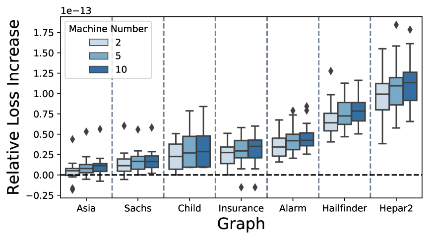
(a) Relative loss distribution.

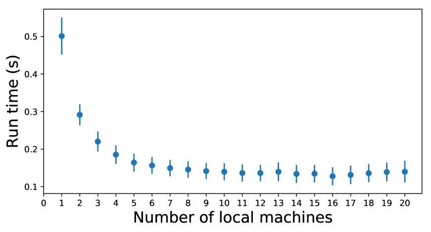
(b) Computation time distribution.

Figure 2: Accuracy and computation time comparison for $f(\pi)$. computation time comparison, with mean and standard deviations plotted, is performed over 20 datasets generated from Insurance.

5.4 Other data generation models

To test the robustness of DARLS against violations of its model assumptions, we also generated data from different DAG models. Particularly, we used threshold-Gaussian and multinomial DAGs to generate discrete data, and then compared DARLS with the other methods.

For the threshold-Gaussian DAG model, we first generated continuous variables $Y_{1},\ldots,Y_{p}$ using Gaussian structural equation models $Y_{j}=B_{j}^{\top}\text{PA}_{j}+\epsilon_{j}$ where $\epsilon_{j}$ is a Gaussian noise from $\mathcal{N}(0,1)$ and each coefficient parameter in $B_{j}\in\mathbb{R}^{s_{j}}$ was sampled uniformly from $[-1.2,-0.8]\leavevmode\nobreak\ \bigcup\leavevmode\nobreak\ [0.8,1.2]$, where $s_{j}=|\text{PA}_{j}|$. Then, we thresheld these continuous values to generate binary data $X_{j}=\mathcal{I}(Y_{j}>c_{j})$, where $c_{j}$ is the sample mean of $Y_{j}$. We used two-component mixture Gaussian to simulate continuous data for root variables in $Y_{j}$, each drawn from $\mathcal{N}(1,1)$ and $\mathcal{N}(-1,1)$ with an equal probability. Under this design, most of the $Y_{j}$’s were bi-modal in distribution, which greatly increased the robustness in thresholding. Such conversion between continuous and categorical variables has been used for modeling BNs in prior work (Lee and Kim 2010; Cai et al. 2020; Song et al. 2021), but the threshold-Gaussian DAG model is not the underlying model for any of six methods in our comparison.

We also simulated multinomial data from contingency tables provided in the BN repository (Scutari 2007). We made a few modifications to the contingency tables to ensure that (1) the number of states per variable was at most three, and (2) the marginal probability of any state was at least $0.1$ for every variable by merging states. Due to the high structure complexity of Hailfinder and Hepar2, the original contingency tables of a few nodes were used without modifications, resulting in marginal probability less than $0.1$ for some states. We note that the multinomial DAG model is the underlying model for the majority of the competing methods, including HC, PC, FGES and MMHC. Therefore, comparisons on these data would also test if the GLDAG model can approximate the multinomial model reasonably well.

Table 2: DARLS against other methods when its model assumption is violated.

Network	Method	threshold-Gaussian								Multinomial
$(p,s_{0})$			TP	R	FP	M		SHD (sd)			TP	R	FP	M		SHD (sd)
Asia	DARLS		6.2	1.6	0.9	0.3		2.8 (3.5)			7.0	0.0	0.1	1.0		1.1 (0.4)
(8,8)	MMHC		1.1	0.7	2.2	6.2		9.1 (1.7)			4.8	1.2	0.5	2.0		3.8 (1.3)
	FGES		0.2	0.8	3.4	6.9		11.1 (1.5)			5.8	2.2	5.0	0.0		7.3 (2.0)
	HC		4.8	2.7	1.4	0.5		4.5 (3.3)			7.8	0.1	0.1	0.0		0.2 (0.9)
	PC		2.2	5.5	6.6	0.3		12.4 (2.1)			2.5	3.5	0.3	2.0		5.8 (0.7)
	NOTEARS		0.6	1.3	4.2	6.1		11.6 (2.0)			0.6	0.9	3.8	6.5		11.2 (1.7)
Sachs	DARLS		7.0	2.9	1.5	7.2		11.5 (3.0)			10.9	3.1	0.1	3.0		6.2 (3.3)
(11, 17)	MMHC		2.0	1.6	1.6	13.4		16.6 (2.5)			3.1	11.2	0.1	2.8		14.0 (1.1)
	FGES		1.6	2.4	2.4	13.1		17.8 (1.9)			4.4	11.8	2.9	0.8		15.5 (4.5)
	HC		6.2	5.2	2.1	5.7		12.9 (2.7)			6.7	5.9	0.0	4.5		10.3 (4.3)
	PC		4.0	8.3	4.9	4.7		17.9 (2.7)			8.8	1.1	0.1	7.0		8.3 (2.5)
	NOTEARS		0.0	2.6	6.0	14.4		23.1 (1.3)			0.1	2.8	5.7	14.2		22.6 (2.4)
Child	DARLS		10.1	9.3	3.7	5.6		18.6 (5.7)			18.1	4.0	0.6	2.9		7.5 (4.3)
(20, 25)	MMHC		3.0	4.2	2.5	17.9		24.5 (2.5)			12.2	8.2	0.5	4.7		13.3 (3.9)
	FGES		1.6	2.8	7.9	20.6		31.4 (2.1)			14.4	9.9	3.9	0.6		14.4 (2.9)
	HC		7.2	13.6	2.4	4.3		20.2 (3.4)			14.9	5.0	0.1	5.0		10.2 (2.3)
	PC		7.8	13.6	31.8	3.5		49.0 (4.4)			6.0	10.8	0.6	8.2		19.6 (2.5)
Insurance	DARLS		11.8	13.2	13.7	26.9		53.8 (8.2)			15.7	16.1	3.5	20.2		39.8 (7.6)
(27, 52)	MMHC		4.3	7.3	9.6	40.4		57.2 (5.8)			16.6	15.2	0.9	20.2		36.3 (2.9)
	FGES		3.0	6.8	16.1	42.1		65.1 (3.9)			23.1	16.6	20.4	12.3		49.2 (6.0)
	HC		8.9	14.8	13.1	28.2		56.1 (4.7)			22.5	10.7	0.8	18.9		30.2 (4.9)
	PC		9.3	20.2	40.2	22.4		82.8 (6.6)			7.3	20.7	0.9	24.0		45.6 (2.8)
Alarm	DARLS		14.4	14.9	8.2	16.6		39.8 (7.4)			18.1	17.6	6.2	10.2		34.0 (4.0)
(37, 46)	MMHC		5.2	4.8	8.2	36.0		48.9 (3.9)			24.6	13.9	2.3	7.4		23.6 (2.6)
	FGES		2.6	1.8	16.1	41.6		59.5 (4.7)			36.6	4.4	25.6	5.0		35.0 (6.0)
	HC		18.9	16.9	9.8	10.2		36.9 (6.1)			27.1	12.3	2.4	6.5		21.2 (4.5)
	PC		10.2	25.6	39.5	10.2		75.2 (4.8)			11.6	25.2	1.8	9.2		36.2 (2.4)
Hailfinder	DARLS		16.5	17.1	11.8	32.4		61.3 (7.9)			16.6	15.2	3.5	34.2		52.9 (5.5)
(56, 66)	MMHC		15.1	4.8	8.4	46.1		59.4 (4.3)			14.3	22.4	4.8	29.3		56.4 (4.1)
	FGES		2.2	1.8	16.6	62.0		80.3 (3.4)			28.1	23.9	17.6	14.0		55.6 (6.3)
	HC		32.9	20.4	9.4	12.7		42.5 (9.2)			23.8	18.0	1.7	24.2		44.0 (2.3)
Hepar2	DARLS		14.8	24.6	27.1	83.7		135.4 (8.6)			18.1	28.6	3.2	76.3		108.1 (4.8)
(70, 123)	MMHC		4.5	12.2	26.2	106.4		144.8 (3.6)			35.0	25.1	51.5	62.9		139.4 (8.7)
	FGES		9.3	6.8	43.4	106.8		157.0 (6.9)			56.8	20.0	74.5	46.2		140.7 (11.0)
	HC		29.8	27.4	25.0	65.8		118.2 (9.4)			28.1	19.8	1.9	75.1		96.8 (7.8)

Table 2 reports the structural estimation accuracy of each method on data generated by the threshold-Gaussian and the mulitnomial DAG models, with $n=10,000$ and $K=20$. When the underlying model is a threshold-Gaussian DAG, DARLS achieved the lowest SHD for 4 networks, i.e. Asia, Sachs, Child and Insurance. For data simulated from multinomial models, DARLS still could estimate the network with the lowest SHD for Sachs and Child. For most of the other cases, DARLS was only worse than HC, but better than or at least comparable to the other methods. Note that we specifically tuned the way for HC to combine local estimates and build a global graph, due to its lack of consensus among local estimates (Remark 1). It is encouraging to see that DARLS uniformly outperformed FGES, a consistent score-based method under the multinomial DAG model (Chickering 2002), highlighting the effectiveness of DARLS in using distributed data. This also suggests that the GLDAG (3) can be a pretty good approximation to the commonly used multinomial DAG model for discrete data. This study confirms that DARLS indeed performs relatively well on data generated from different DAG models, which is important for its practical use. This is further demonstrated by the application to a real dataset in next section.

6 Real data application

In this section, we apply our method to the ChIP-Seq data generated by Chen et al. (2008). The dataset contains the DNA binding sites of 12 transcription factors (TFs) in mouse embryonic stem cells: Smad1, Stat3, Sox2, Pou5f1, Nanog, Esrrb, Tcfcp2l1, Klf4, Zfx, E2f1, Myc, and Mycn. For each TF, an association strength score, which is the weighted sum of the corresponding ChIP-Seq signal strength, was calculated for each of the 18,936 genes (Ouyang et al. 2009). Roughly speaking, this score can be understood as a measure of the binding strength of a TF to a gene. Following the same preprocessing in Wang and Zhou (2021), the genes with zero association scores were removed from our analysis. Accordingly, our observed data matrix, of size $n\times p=8462\times 12$, contains the association scores of 12 TFs over 8,462 genes. We aim to build a causal network that reveals how these 12 TFs affect each other’s binding to genes. The associate scores of a TF are typically bimodal, and they were discretized before network estimation; see Figure LABEL:fig:chip-dis-example in the supplemental material for illustration of the discretization.

We distributed this dataset across $K=20$ local machines and applied DARLS, HC, MMHC, PC and FGES to the distributed data to learn the protein-DNA binding network. NOTEARS was excluded because its performance was not competitive. Local estimates of a competing method were combined to construct a global graph as we did in Section 5. To ease the comparison, we controlled the sparsity of estimated networks such that every method produced two graphs using the distributed data, with roughly $\widehat{s}_{0}=17$ and 29 edges, except FGES which had difficulty generating output close to 17 edges. We also applied each method on the combined data (i.e, $K=1$) with the same parameters in Section 5. In this case, each estimated graph had around $\widehat{s}_{0}=30$ edges. The only exception is PC, whose estimate had 21 edges even when its significance level had been reduced to $10^{-10}$.

Since the true network structure is unknown, test data likelihood under multinomial DAG models in ten-fold cross validation is used to assess the accuracy of estimated networks. Denote by $\widetilde{g}$ and $g$ the likelihood values using training and test datasets, respectively, under multinomial DAG models (see supplemental material Section LABEL:sec:chip-likelihood for calculation of $\widetilde{g}$ and $g$). We also compute $\text{BIC}=-2\log\widetilde{g}+\log(\widetilde{n})\mathcal{N}(\widehat{\mathcal{G}})$ for model comparison, where $\widetilde{n}$ is the training sample size and $\mathcal{N}(\widehat{\mathcal{G}})$ is the number of multinomial parameters for estimated graph $\widehat{\mathcal{G}}$. We choose some benchmarks to ease comparison. Denote by $g_{\text{B}}$ and $\text{BIC}_{\text{B}}$ the highest test data likelihood and the lowest BIC value, respectively. Define the log-likelihood difference $\Delta(\log g)=\log g-\log g_{\text{B}}$ and the BIC difference $\Delta\text{BIC}=\text{BIC}-\text{BIC}_{\text{B}}$. Note that since $\log g$ is test data log-likelihood while BIC is calculated with training data, the magnitude of $\Delta\text{BIC}$ is much larger than $\Delta(\log g)$. We also compute the value of $\exp{\{-\Delta\text{BIC}/(2\widetilde{n})\}}$ as an approximation to the normalized marginal likelihood ratio (NLR) $(P(\widetilde{X}\mid\widehat{\mathcal{G}})/P(\widetilde{X}\mid\widehat{\mathcal{G}}_{B}))^{1/\widetilde{n}}$, where $\widetilde{X}$ denotes training data, between estimated DAGs $\widehat{\mathcal{G}}$ by a competing method and $\widehat{\mathcal{G}}_{B}$ by the BIC benchmark.

Table 3 summarizes $\widehat{s}_{0}$, $\Delta(\log g)$, $\Delta\text{BIC}$ and NLR of each method under three comparison settings, namely sparse, moderate and combined. The first two settings report results with different degree of sparsity in estimated graphs using distributed data over $K=20$ machines, and the last one shows results using combined data (i.e., $K=1$). In both sparse and moderate settings, DARLS achieves the highest test data likelihood and the smallest BIC, outperforming all the other methods by a substantial margin, which again demonstrates its effectiveness in DAG learning with distributed data. When applied to combined data, all methods, except PC, have higher test data likelihood than on distributed data, and the test data likelihood values are quite comparable. Comparing the likelihood between combined and distributed data for each method, we see that DARLS shows the smallest difference. In other words, among all the methods, DARLS has the smallest loss when applied to distributed data as compared to its result on the combined data.

It is worth mentioning that the likelihood for each method is calculated under the multinomial DAG model, instead of the GLDAG model. Thus, the superior performance of the distributed learning by DARLS on this real-world data suggests that our proposed GLDAG model is a good approximation to the underlying data generation mechanism.

Table 3: Comparison on the ChIP-Seq dataset. Best performance of each case is in bold.

Method	Sparse							Moderate							Combined
	$\widehat{s}_{0}$		$\Delta(\log g)$		$\Delta\text{BIC}$	NLR		$\widehat{s}_{0}$		$\Delta(\log g)$		$\Delta\text{BIC}$	NLR		$\widehat{s}_{0}$		$\Delta(\log g)$		$\Delta\text{BIC}$	NLR
DARLS	16.5		$\mathbf{-136.9}$		$\mathbf{1051.6}$	0.501		27.5		$\mathbf{-22.4}$		$\mathbf{297.7}$	0.822		31.0		$-$3.7		540.2	0.701
MMHC	17.0		$-$149.6		2470.0	0.198		29.5		$-$44.4		1062.4	0.498		30.0		$-$1.7		$\mathbf{0.0}$	1.000
FGES	11.5		$-$164.3		2478.5	0.196		28.0		$-$39.6		1026.6	0.510		34.0		$-$2.7		250.9	0.848
HC	17.0		$-$151.9		2510.1	0.192		29.0		$-$36.8		1174.9	0.462		30.0		$\mathbf{0.0}$		7.9	0.995
PC	17.0		$-$156.3		2510.1	0.192		29.0		$-$36.9		942.6	0.538		21.0		$-$77.1		1047.8	0.503

Figure 3: DAG (left) and the converted CPDAG (right) learned by DARLS.

To gain more scientific insights, we show in Figure 3 the sparser DAG ($\widehat{s}_{0}=17$) and its converted CPDAG, learned by DARLS from the full dataset ($n=8,462$) distributed over $K=20$ local machines, with $\lambda=0.06$ and refinement parameter $\alpha=0.3$. An interesting observation is the directed path Nanog$\to$Pou5f1$\to$Sox2 in the estimated CPDAG, among the three core regulators in the gene regulatory network in mouse embryonic stem cells (Chen et al. 2008; Zhou et al. 2007). It is well-known that many genes are co-regulated by Pou5f1, Sox2 and Nanog. The estimated path suggests that Nanog binding would cause the binding of Pou5f1, which then may cause Sox2 binding. This provides new clue for how the three TFs work together to co-regulate downstream genes. Data analysis in Chen et al. (2008), the original work that generated the ChIP-Seq data, suggests that there are two clusters of TFs that tend to co-bind: The first group consists of Nanog, Sox2, Oct4, Smad1 and STAT3, while the second group includes Mycn, Myc, Zfx and E2f1. These two groups are clearly recovered in the estimated CPDAG, which contains a dense undirected subgraph on the second group of TFs and a fully directed subgraph on the first group. Moreover, the directed edge Myc$\to$Pou5f1 indicates that the second group might be in the causal upstream of the first group, a novel hypothesis for potential experimental investigation.

7 Discussion

In this paper, we develop the DARLS algorithm that incorporates a distributed optimization method in simulated annealing to learn causal graphs from distributed data. Based on simulation studies and a real data application, we have shown that DARLS is highly competitive even when its model assumptions are violated. In its distributed optimization given an ordering, DARLS learns a causal graph by optimizing a convex penalized likelihood. In practice, one may consider concave penalties (Aragam and Zhou 2015; Ye et al. 2021) to improve accuracy when learning DAGs, although there may be lack of theoretical guarantees for convergence of distributed learning with a concave penalty. This is certainly a promising further development for our method.

Our proposed GLDAG model includes a family of flexible distributions besides linear Gaussian models (with equal variance), and thus can be applied to different types of data. It is also possible to add interaction terms to GLDAGs (3) to model nonlinear effects between variables. Such generalization is expected to approximate real causal relations with higher accuracy. We have established that continuous GLDAGs are identifiable, justifying their use in causal discovery, and it is left as future work to study the identifiability of general GLDAGs.

The primary focus of this paper is on big distributed data, with large $n$ but moderate $p$. In this setting, we established the convergence of the solution obtained by distributed optimization to a global minimizer of the loss using the combined data, and the consistency of the global minimizer as an estimate of the true DAG parameter. However, generalizing the convergence and consistency results to allow diverging $p$ is theoretically interesting and left as future work.

References

- Apple and Google (2021) Apple and Google (2021), “Explosure Notification Privacy-preserving Analytics (ENPA) White Paper,” Tech. rep., Apple and Google.
- Aragam et al. (2019) Aragam, B., Gu, J., and Zhou, Q. (2019), “Learning Large-Scale Bayesian Networks with the sparsebn Package,” Journal of Statistical Software, 91, 1–38.
- Aragam and Zhou (2015) Aragam, B. and Zhou, Q. (2015), “Concave Penalized Estimation of Sparse Gaussian Bayesian Networks,” Journal of Machine Learning Research, 16, 2273–2328.
- Cai et al. (2020) Cai, Q., Kang, J., and Yu, T. (2020), “Bayesian Network Marker Selection via the Thresholded Graph Laplacian Gaussian Prior,” Bayesian Analysis, 15, 79–102.
- Chen et al. (2008) Chen, X., Xu, H., Yuan, P., Fang, F., Huss, M., Vega, V. B., Wong, E., Orlov, Y. L., Zhang, W., Jiang, J., Loh, Y.-H., Yeo, H. C., Yeo, Z. X., Narang, V., Govindarajan, K. R., Leong, B., Shahab, A., Ruan, Y., Bourque, G., Sung, W.-K., Clarke, N. D., Wei, C.-L., and Ng, H.-H. (2008), “Integration of External Signaling Pathways with the Core Transcriptional Network in Embryonic Stem Cells,” Cell, 133, 1106–17.
- Chickering (2002) Chickering, D. M. (2002), “Optimal Structure Identification with Greedy Search,” Journal of Machine Learning Research, 3, 507–554.
- Dehejia and Wahba (1999) Dehejia, R. H. and Wahba, S. (1999), “Causal Effects in Nonexperimental Studies: Reevaluating the Evaluation of Training Programs,” Journal of the American Statistical Association, 94, 1053–1062.
- Fan et al. (2019) Fan, J., Guo, Y., and Wang, K. (2019), “Communication-Efficient Accurate Statistical Estimation,” arXiv:1906.04870.
- Friedman and Koller (2003) Friedman, N. and Koller, D. (2003), “Being Bayesian about Network Structure. A Bayesian Approach to Structure Discovery in Bayesian Networks,” Machine Learning, 50, 95–125.
- Fu and Zhou (2013) Fu, F. and Zhou, Q. (2013), “Learning Sparse Causal Gaussian Networks with Experimental Intervention: Regularization and Coordinate Descent,” Journal of the American Statistical Association, 108, 288–300.
- Gámez et al. (2011) Gámez, J. A., Mateo, J. L., and Puerta, J. M. (2011), “Learning Bayesian Networks by Hill Climbing: Efficient Methods Based on Progressive Restriction of the Neighborhood,” Data Mining and Knowledge Discovery, 22, 106–148.
- Glymour (2006) Glymour, M. M. (2006), “Using Causal Diagrams to Understand Common Problems in Social Epidemiology,” in Methods in Social Epidemiology, John Wiley and Sons, pp. 393–428.
- Gou et al. (2007) Gou, K. X., Jun, G. X., and Zhao, Z. (2007), “Learning Bayesian Network Structure from Distributed Homogeneous Data,” Eighth ACIS International Conference on Software Engineering, Artificial Intelligence, Networking, and Parallel/Distributed Computing, 3, 250–254.
- Gu et al. (2019) Gu, J., Fu, F., and Zhou, Q. (2019), “Penalized Estimation of Directed Acyclic Graphs from Discrete Data,” Statistics and Computing, 29, 161–176.
- Guo et al. (2020) Guo, R., Cheng, L., Li, J., Hahn, P. R., and Liu, H. (2020), “A Survey of Learning Causality with Data: Problems and Methods,” ACM Computing Surveys, 53, 1–37.
- Heckerman et al. (1995) Heckerman, D., Geiger, D., and Chickering, D. M. (1995), “Learning Bayesian Networks: The Combination of Knowledge and Statistical Data,” Machine Learning, 20, 197–243.
- Hill (2012) Hill, J. L. (2012), “Bayesian Nonparametric Modeling for Causal Inference,” Journal of Computational and Graphical Statistics, 20, 217–240.
- Hoyer et al. (2008) Hoyer, P. O., Janzing, D., Mooij, J., Peters, J., and Schölkopf, B. (2008), “Nonlinear Causal Discovery with Additive Noise Models,” Preceedings of 21st International Conference on Neural Information Processing Systems, 689–696.
- Imbens (2004) Imbens, G. W. (2004), “Nonparametric Estimation of Average Treatment Effects under Exogeneity: A Review,” The Review of Economics and Statistics, 86, 4–29.
- Jordan et al. (2018) Jordan, M. I., Lee, J. D., and Yang, Y. (2018), “Communication-Efficient Distributed Statistical Inference,” Journal of the American Statistical Association, 114, 668–681.
- Kalisch et al. (2012) Kalisch, M., M’́achler, M., Colombo, D., Maathuis, M. H., and B’́uhlmann, P. (2012), “Causal Inference Using Graphical Models with the R Package pcalg,” Journal of Statistical Software, 47, 1–26.
- Larrañaga et al. (1996) Larrañaga, P., Poza, M., Yurramendi, Y., Murga, R. H., and Kuijpers, C. M. H. (1996), “Structure Learning of Bayesian Networks by Genetic Algorithms: A Performance Analysis of Control Parameters,” IEEE Transactions on Pattern Analysis and Machine Intelligence, 18, 912–926.
- Lee and Kim (2010) Lee, N. and Kim, J.-M. (2010), “Conversion of Categorical Variables into Numerical Variables via Bayesian Network Classifiers for Binary Classifications,” Computational Statistics Harold & Maude Data Analysis, 54, 1247–1265.
- Meek (1995) Meek, C. (1995), “Strong Completeness and Faithfulness in Bayesian Networks,” Proceedings of the Eleventh conference on Uncertainty in artificial intelligence, 411–418.
- Mehmood et al. (2016) Mehmood, A., Natgunanathan, I., Xiong, Y., Hua, G., and Guo, S. (2016), “Protection of Big Data Privacy,” IEEE Access, 4, 1821–1834.
- Molzahn et al. (2017) Molzahn, D. K., Dörfler, F., Sandberg, H., Low, S. H., Chakrabarti, S., Baldick, R., and Lavaei, J. (2017), “A Survey of Distributed Optimization and Control Algorithms for Electric Power Systems,” IEEE Transactions on Smart Grid, 8, 2941–2962.
- Na and Yang (2010) Na, Y. and Yang, J. (2010), “Distributed Bayesian Network Structure Learning,” IEEE International Symposium on Industrial Electronics, 1607–1611.
- Ouyang et al. (2009) Ouyang, Z., Zhou, Q., and Wong, W. H. (2009), “ChIP-Seq of Transcription Factors Predicts Absolute and Differential Gene Expression in Embryonic Stem Cells,” Preceedings of the National Academic of Science of the United State of America, 106, 21521–6.
- Parikh and Boyd (2013) Parikh, N. and Boyd, S. (2013), “Proximal Algorithms,” Foundations and Trends in Optimization, 1, 123–231.
- Pearl (1995) Pearl, J. (1995), “Causal Diagrams for Empirical Research,” Biometrika, 82, 669–710.
- Pearl (2009) — (2009), “Causal Inference in Statistics: An Overview,” Statistical Surveys, 3, 96–146.
- Peters and Bühlmann (2014) Peters, J. and Bühlmann, P. (2014), “Identifiability of Gaussian Structural Models with Equal Error Variances,” Biometrika, 101, 219–228.
- Peters et al. (2014) Peters, J., Mooij, J. M., Janzing, D., and Schölkopf, B. (2014), “Causal Discovery with Continuous Additive Noise Models,” Journal of Machine Learning Research, 15, 2009–2053.
- Ramanan and Natarajan (2020) Ramanan, N. and Natarajan, S. (2020), “Causal Learning from Predictive Modeling for Observational Data,” Frontiers in Big Data, 3, 535976.
- Ramsey et al. (2017) Ramsey, J., Glymour, M., Sanchez-Romero, R., and Glymour, C. (2017), “A Million Variables and More: the Fast Greedy Equivalence Search Algorithm for Learning High-dimensional Graphical Causal Models, with an Application to Functional Magnetic Resonance Images,” International Journal of Data Science and Analytics, 3, 121–129.
- Scanagatta et al. (2015) Scanagatta, M., de Campos, C. P., Corani, G., and Zaffalon, M. (2015), “Learning Bayesian Networks with Thousands of Variables,” in Advances in Neural Information Processing Systems, 1864–1872.
- Scutari (2007) Scutari, M. (2007), “Bayesian Network Repository,” http://www.bnlearn.com/bnrepository/, accessed: 2020-05-01.
- Scutari (2010) — (2010), “Learning Bayesian Networks with the bnlearn R Package,” Journal of Statistical Software, 35, 1–22.
- Shamir et al. (2014) Shamir, O., Srebro, N., and Zhang, T. (2014), “Communication-Efficient Distributed Optimization using an Approximate Newton-type Method,” Proceedings of the 31st International Conference on International Conference on Machine Learnings, 32, 1000–1008.
- Shimizu et al. (2006) Shimizu, S., Hoyer, P. O., Hyvärinen, A., and Kerminen, A. (2006), “A Linear Non-Gaussian Acyclic Model for Causal Discovery,” Journal of Machine Learning Research, 7, 2003–2030.
- Song et al. (2021) Song, Y., Zhou, X., Kang, J., Aung, M. T., Zhang, M., Zhao, W., Needham, B. L., Kardia, S. L. R., Liu, Y., Meeker, J. D., Smith, J. A., and Mukherjee, B. (2021), “Bayesian Sparse Mediation Analysis with Targeted Penalization of Natural Indirect Effects,” Journal of the Royal Statistical Society. Series C, Applied statistics, 70, 1391–1412.
- Spirtes and Glymour (1991) Spirtes, P. and Glymour, C. (1991), “An Algorithm for Fast Recovery of Sparse Causal Graphs,” Social Science Computer Review, 9, 62–72.
- Tang et al. (2019) Tang, Y., Wang, J., Nguyen, M., and Altintas, I. (2019), “PEnBayes: A Multi-Layered Ensemble Approach for Learning Bayesian Network Structure from Big Data,” Sensors, 19, 4400.
- Tsamardinos et al. (2006) Tsamardinos, I., Brown, L. E., and Aliferis, C. F. (2006), “The Max-Min Hill-Climbing Bayesian Network Structure Learning Algorithm,” Machine Learning, 65, 31–78.
- Wang and Zhou (2021) Wang, B. and Zhou, Q. (2021), “Causal Network Learning with N0n-intertible Functional Relationships,” Computational Statistics and Data Analysis, 156, 107141.
- Yang et al. (2019) Yang, T., Yi, X., Wu, J., Yuan, Y., Wu, D., Meng, Z., Hong, Y., Wang, H., Lin, Z., and Johansson, K. H. (2019), “A Survey of Distributed Optimization,” Annual Reviews in Control, 47, 278–305.
- Ye et al. (2021) Ye, Q., Amini, A. A., and Zhou, Q. (2021), “Optimizing Regularized Cholesky Score for Order-Based Learning of Bayesian Networks,” IEEE Transactions on Pattern Analysis & Machine Intelligence, 43, 3555–3572.
- Yuan and Lin (2007) Yuan, M. and Lin, Y. (2007), “Model Selection and Estimation in Regression with Grouped Variables,” Journal of Royal Statistical Society, Series B, 68, 49–67.
- Zhang et al. (2013) Zhang, Y., Duchi, J. C., and Wainwright, M. J. (2013), “Communication-Efficient Algorithms for Statistical Optimization,” Journal of Machine Learning Research, 14, 3321–3363.
- Zheng (2018) Zheng, X. (2018), “DAGs with NO TEARS,” https://github.com/xunzheng/notearss, accessed: 2021-09-01.
- Zheng et al. (2018) Zheng, X., Aragam, B., Pavikumar, P., and Xing, E. P. (2018), “DAGs with NO TEARS: Continuous Optimization for Structure Learning,” in Advances in Neural Information Processing Systems.
- Zhou et al. (2007) Zhou, Q., Chipperfield, H., Melton, D. A., and Wong, W. H. (2007), “A Gene Regulatory Network in Mouse Embryonic Stem Cells,” Preceedings of the National Academy of Sciences of the United States of America, 104, 16438–16443.
- Zinkevich et al. (2010) Zinkevich, M. A., Weimer, M., Smola, A., and Li, L. (2010), “Parallelized Stochastic Gradient Descent,” in Advances in Neural Information Processing Systems, vol. 23, pp. 2595–2603.