The Hilbert Space of large $N$ Chern-Simons matter theories

Abstract

We demonstrate that the known expressions for the thermal partition function of large $N$ Chern-Simons matter theories admit a simple Hilbert space interpretation as the partition function of an associated ungauged large $N$ matter theory with one additional condition: the Fock space of this associated theory is projected down to the subspace of its quantum singlets i.e. singlets under the Gauss law for Chern-Simons gauge theory. Via the Chern-Simons / WZW correspondence, the space of quantum singlets are equivalent to the space of WZW conformal blocks. One step in our demonstration involves recasting the Verlinde formula for the dimension of the space of conformal blocks in $SU(N)_{k}$ and $U(N)_{k,k^{\prime}}$ WZW theories into a simple and physically transparent form, which we also rederive by evaluating the partition function and superconformal index of pure Chern-Simons theory in the presence of Wilson lines. A particular consequence of the projection of the Fock space of Chern-Simons matter theories to quantum (or WZW) singlets is the ‘Bosonic Exclusion Principle’: the number of bosons occupying any single particle state is bounded above by the Chern-Simons level. The quantum singlet condition (unlike its Yang-Mills Gauss Law counterpart) has a nontrivial impact on thermodynamics even in the infinite volume limit. In this limit the projected Fock space partition function reduces to a product of partition functions, one for each single particle state. These single particle state partition functions are $q$-deformations of their free boson and free fermion counterparts and interpolate between these two special cases. We also propose a formula for the large $N$ partition function that is valid for arbitrary finite volume of the spatial $S^{2}$ and not only at large volume.

1 Introduction

$SU(N)_{k}$ Chern-Simons theories (and their $U(N)$ cousins) coupled to fundamental matter turn out to be effectively solvable in the ’t Hooft large $N$ limit

$$N\to\infty\ ,\quad k\to\infty\ ,\quad\text{with}\quad\lambda=\frac{N}{\kappa}\quad\text{fixed}\ ,\quad\text{with}\quad\kappa=k+\text{sgn}(k)N\ .$$ (1)

The study of these theories in the ’t Hooft limit has led to several qualitative insights including the discovery of Bose-Fermi duality in these theories Sezgin:2002rt ; Klebanov:2002ja ; Giombi:2009wh ; Benini:2011mf ; Giombi:2011kc ; Aharony:2011jz ; Maldacena:2011jn ; Maldacena:2012sf ; Chang:2012kt ; Jain:2012qi ; Aharony:2012nh ; Yokoyama:2012fa ; GurAri:2012is ; Aharony:2012ns ; Jain:2013py ; Takimi:2013zca ; Jain:2013gza ; Yokoyama:2013pxa ; Bardeen:2014paa ; Jain:2014nza ; Bardeen:2014qua ; Gurucharan:2014cva ; Dandekar:2014era ; Frishman:2014cma ; Moshe:2014bja ; Aharony:2015pla ; Inbasekar:2015tsa ; Bedhotiya:2015uga ; Gur-Ari:2015pca ; Minwalla:2015sca ; Radicevic:2015yla ; Geracie:2015drf ; Aharony:2015mjs ; Yokoyama:2016sbx ; Gur-Ari:2016xff ; Karch:2016sxi ; Murugan:2016zal ; Seiberg:2016gmd ; Giombi:2016ejx ; Hsin:2016blu ; Radicevic:2016wqn ; Karch:2016aux ; Giombi:2016zwa ; Wadia:2016zpd ; Aharony:2016jvv ; Giombi:2017rhm ; Benini:2017dus ; Sezgin:2017jgm ; Nosaka:2017ohr ; Komargodski:2017keh ; Giombi:2017txg ; Gaiotto:2017tne ; Jensen:2017dso ; Jensen:2017xbs ; Gomis:2017ixy ; Inbasekar:2017ieo ; Inbasekar:2017sqp ; Cordova:2017vab ; Charan:2017jyc ; Benini:2017aed ; Aitken:2017nfd ; Jensen:2017bjo ; Chattopadhyay:2018wkp ; Turiaci:2018nua ; Choudhury:2018iwf ; Karch:2018mer ; Aharony:2018npf ; Yacoby:2018yvy ; Aitken:2018cvh ; Aharony:2018pjn ; Dey:2018ykx ; Chattopadhyay:2019lpr ; Dey:2019ihe ; Halder:2019foo ; Aharony:2019mbc ; Li:2019twz ; Jain:2019fja ; Inbasekar:2019wdw ; Inbasekar:2019azv ; Jensen:2019mga ; Kalloor:2019xjb ; Ghosh:2019sqf ; Inbasekar:2020hla ; Jain:2020rmw ; Minwalla:2020ysu ; Jain:2020puw ; Mishra:2020wos ; Jain:2021wyn ; Jain:2021vrv ; Gandhi:2021gwn ; toappear1 .

1.1 The question posed in this paper

One of the earliest explicit large $N$ computations in Chern-Simons matter theories was that of the thermal partition function on an $S^{2}$ whose volume $\mathcal{V}_{2}$ is taken to scale like $N$ with all other quantities held fixed (e.g. masses, the temperature $T$, chemical potential $\mu$). The large $N$ computations of the thermal partition function (see Giombi:2011kc ; Jain:2012qi ; Yokoyama:2012fa ; Aharony:2012ns ; Jain:2013py ; Yokoyama:2013pxa ; Choudhury:2018iwf ; Dey:2018ykx ; Dey:2019ihe ; Halder:2019foo ; Minwalla:2020ysu ) was accomplished by evaluating the (chemical potential twisted) Euclidean partition function $\mathcal{Z}$ of the relevant theories on $S^{2}\times S^{1}$. The purpose of this paper is to give a Hilbert space interpretation of these known results, i.e. to construct a Hilbert space ${\cal H}$ and a simple effective Hamiltonian $H$ (and conserved charge $Q$) so that the previously obtained path integral expression for $\mathcal{Z}$ can be written as

$$\mathcal{Z}={\rm Tr}_{{\cal H}}\ \text{e}^{-\beta\left(H-\mu Q\right)}\ .$$ (2)

Restated, the aim of this paper is to construct an effective Hilbert space and Hamiltonian that reproduces the known thermodynamics of large $N$ Chern-Simons matter theories.

1.2 A simpler analogous question and its answer

To explain the nature of the question posed in this paper (together with elements of its answer) we briefly recall an analogous question in a more familiar and simpler setting. Consider the $S^{2}\times S^{1}$ partition function of an $SU(N)$ Yang-Mills theory in the weak coupling limit $g^{2}_{YM}\to 0$. In this (almost) free problem it is easy to directly evaluate the $S^{2}\times S^{1}$ path integral. This problem was addressed by the authors of Sundborg:1999ue ; Aharony:2003sx who demonstrated that the final answer to this partition function takes the form of a simple integral over a single $N\times N$ unitary matrix $U$:

$$\mathcal{I}_{\rm cl}=\int dU~{}{\rm Tr}_{{\cal H}_{\rm Fock}}\left(\widehat{U}\text{e}^{-\beta H}\right)\ .$$ (3)

$U$ in (3) is the zero mode (on $S^{2}$) of the holonomy of the gauge field around the time circle. The integrand on the RHS of (3) is the trace over the free Fock Space $\mathcal{H}_{\rm Fock}$ which is obtained from zero coupling Yang-Mills theory on $S^{2}$ without imposing the Gauss law of $\text{e}^{-\beta{H}}$ twisted by $\widehat{U}$, the operator on $\mathcal{H}_{\rm Fock}$ corresponding to the holonomy $U$, and ${H}$ is the Hamiltonian on this Fock space.

The analog of the question posed in the previous subsection is the following: can we identify a Hilbert Space ${\cal H}_{\rm cl}$ and a Hamiltonian ${H}_{0}$ such that

$${\rm Tr}_{{\cal H}_{\rm cl}}\left(\text{e}^{-\beta{H}_{0}}\right)=\int dU~{}{\rm Tr}_{{\cal H}_{\rm Fock}}\left(\hat{U}\text{e}^{-\beta H}\right)\ .$$ (4)

In this simple context the answer to this question is both well known (see Sundborg:1999ue ; Aharony:2003sx ) and easy to guess. The integral over $U$ in (3) simply projects the Fock space $\mathcal{H}_{\rm Fock}$ onto its $SU(N)$ invariant sector Sundborg:1999ue ; Aharony:2003sx (see Appendix A for a description of the formula for the number of singlets). It follows that the Hilbert space ${\cal H}_{\rm cl}$ must be identified with this $SU(N)$ invariant sector, and $H_{0}$ is the restriction of the free Fock space Hamiltonian ${H}$ down to the $SU(N)$ singlet sector.

We emphasize that while the Hilbert Space ${\cal H}_{\rm cl}$ is the projection of a Fock space, it is not by itself a Fock space. The projector onto singlets is an - indeed the only - ‘interaction’ in the system.

1.3 The Hilbert space of a Chern-Simons matter theory: an example

In this paper we address a question similar to that posed in Section 1.2, but in the more complicated context of Chern-Simons matter theories. In order to explain our answer in an intelligible manner, in this subsection we outline the question in some technical detail and work towards obtaining its answer in the context of an example viz. the regular boson theory in its unHiggsed phase.

1.3.1 The theory

The ‘regular boson’ theory is a theory of $N$ complex bosons in three spacetime dimensions whose (power counting renormalizable) interactions preserve $U(N)$ invariance. The $U(N)$ global symmetry of this theory (or an $SU(N)$ subgroup thereof, depending on details) is then gauged, and the self-interactions of the gauge field are governed by a Chern-Simons action. For concreteness, we work with an $SU(N)_{k}$ Chern-Simons gauge theory.

Working in the dimensional regularization scheme, the Euclidean action for this theory is given by

$$\mathcal{S}[A,\phi]=\mathcal{S}_{\rm CS}[A]+\int d^{3}x\left(\overline{D_{\mu}\phi}D_{\mu}\phi+V_{{\rm cl}}(\phi)\right)\ ,$$ (5)

where $D_{\mu}$ is the gauge covariant derivative, $\mathcal{S}_{\rm CS}[A]$ is the Chern-Simons action for the gauge field and the potential $V_{{\rm cl}}(\phi)$ is given by

$$V_{\rm cl}(\phi)=m_{B}^{2}\bar{\phi}\phi+\frac{4\pi b_{4}}{\kappa_{B}}(\bar{\phi}\phi)^{2}+\frac{(2\pi)^{2}}{\kappa_{B}^{2}}(x_{6}^{B}+1)(\bar{\phi}\phi)^{3}\ .$$ (6)

1.3.2 A theory of interacting bosons

As Chern-Simons gauge fields have no propagating degrees of freedom in the bulk, the regular boson theory on $S^{2}$ may be thought of as a theory of matter fields with interactions induced by integrating out the gauge fields. In particular, integrating out the gauge fields results in a renormalization of the classical effective potential of the theory.

In Dey:2018ykx , the exact large $N$ quantum effective potential for the operator ${\bar{\phi}}\phi$ was computed. This renormalized potential in the unHiggsed phase can be read off from the result of Dey:2018ykx :

$$V({\bar{\phi}}\phi)=m_{B}^{2}\bar{\phi}\phi+\frac{4\pi b_{4}}{\kappa_{B}}(\bar{\phi}\phi)^{2}+\frac{(2\pi)^{2}}{\kappa_{B}^{2}}(x_{6}^{B}+\tfrac{4}{3})(\bar{\phi}\phi)^{3}\ .$$ (7)

Consequently, the large $N_{B}$ regular boson theory may be viewed as a theory of $N_{B}$ complex bosons, interacting via the potential (7), plus other (as yet unspecified) nonlocal interactions that have their origin in gauge boson exchange.

1.3.3 $S^{2}$ thermal partition function ignoring the nonlocal interactions

As a first approximation to the partition function of our theory, we simply ignore all nonlocal interactions and compute the partition function of the scalar theory interacting via the potential (7), i.e. of the theory

$$\mathcal{S}[\phi]=\int d^{3}x\Bigg{(}\partial_{\mu}\bar{\phi}\partial^{\mu}\phi+m_{B}^{2}\bar{\phi}\phi+\frac{4\pi b_{4}}{\kappa_{B}}(\bar{\phi}\phi)^{2}+\frac{(2\pi)^{2}}{\kappa_{B}^{2}}(x_{6}^{B}+\tfrac{4}{3})(\bar{\phi}\phi)^{3}\Bigg{)}\ .$$ (8)

The computation is a simple exercise. We introduce two new Lagrange multiplier fields $c_{B}^{2}$ and $\sigma_{B}$ and rewrite (8) as

$$\mathcal{S}[c_{B},\sigma_{B},\phi]$$

$$\quad=\int d^{3}x\left(\partial_{\mu}\bar{\phi}\partial^{\mu}\phi+c_{B}^{2}\bar{\phi}\phi+\frac{N_{B}}{2\pi}\left((m_{B}^{2}-c_{B}^{2})\sigma_{B}+2\lambda_{B}b_{4}\sigma_{B}^{2}+\lambda_{B}^{2}(x_{6}^{B}+\tfrac{4}{3})\sigma_{B}^{3}\right)\right)\ ,$$

$$\quad=\int d^{3}x\left(\partial_{\mu}\bar{\phi}\partial^{\mu}\phi+c_{B}^{2}\bar{\phi}\phi+F_{\rm RB,int}(c_{B},\sigma_{B})\right)\ ,$$ (9)

where $\lambda_{B}=N_{B}/\kappa_{B}$ and we have defined the quantity $F_{\rm RB,int}$ by the last equality. Note that the term $F_{\rm RB,int}(c_{B},\sigma_{B})$ in the last line of (1.3.3) is a simple rewriting of the contact terms in (8) in terms of the new variable $\sigma_{B}$.

In the large $N$ limit, $c_{B}^{2}$ and $\sigma_{B}$ are frozen at their saddle point values. Under the plausible assumption of translational invariance of the thermal ensemble, these saddle point values are constants. At fixed values of $c^{2}_{B}$ and $\sigma_{B}$, the scalar field $\phi$ is a free boson of squared mass $c_{B}^{2}$. Integrating out the field $\phi$ yields

$$\text{Tr}_{\mathcal{H}_{B,\rm Fock}}\left(\text{e}^{-\beta(H-\mu Q)}\right)\ ,$$ (10)

where $\mathcal{H}_{B,\rm Fock}$ is the Fock space of a free scalar field of squared-mass $c_{B}^{2}$. It follows that the $S^{2}\times S^{1}$ partition function of the theory governed by the action (1.3.3) at large $N$ is given by

$$\mathcal{Z}^{\rm ungauged\ RB}_{S^{2}\times S^{1}}=\text{Ext}_{\{\sigma_{B},c_{B}\}}\left[\text{e}^{-\mathcal{V}_{2}\beta F_{\rm RB,int}(c_{B},\sigma_{B})}\ \text{Tr}_{\mathcal{H}_{B,\rm Fock}}\left(\text{e}^{-\beta(H-\mu Q)}\right)\right]\ .$$ (11)

where $\text{Ext}_{\{\sigma_{B},c_{B}\}}$ denotes extremizing the result over $c_{B}$ and $\sigma_{B}$.

1.3.4 Accounting for the Gauss law

Equation (11) yields the partition function of the regular boson theory after ignoring the effect of gauge boson mediated nonlocal interactions. However gauge theories on compact manifolds always include at least one nonlocal interaction viz. the Gauss law. Inspired by Section 1.2, we might attempt to account for the Gauss law by replacing the Fock space partition function in (2.2.2) by its projection onto the space of ‘classical’ $SU(N)$ singlets, i.e. by

$$\mathcal{Z}^{\rm Gauss\ RB}_{S^{2}\times S^{1}}=\text{Ext}_{\{\sigma_{B},c_{B}\}}\left[\text{e}^{-\mathcal{V}_{2}\beta F_{\rm RB,int}(c_{B},\sigma_{B})}\ \int dU~{}\text{Tr}_{\mathcal{H}_{B,\rm Fock}}\left(\widehat{U}\text{e}^{-\beta(H-\mu Q)}\right)\right]\ .$$ (12)

where $U$ is a constant $SU(N)$ matrix and $\widehat{U}$ is the operator corresponding to $U$ that acts on $\mathcal{H}_{B,\rm Fock}$, as in Section 1.2. However, (12) accounts for the nonlocal gauge-mediated interactions of the Chern-Simons matter theories only in a crude approximation, and so is not the exact answer for the thermal partition function of the theory in the large $N_{B}$ limit.

1.3.5 The actual partition function

Fortunately, as we have mentioned before, the exact large $N_{B}$ result of the thermal partition function of this theory is known. While this exact answer (presented in (2.2.2)) differs from that presented in (12), it has many similarities to that naive guess. Indeed in this paper we demonstrate that this exact answer, (2.2.2), can be rewritten in the form

$$\mathcal{Z}^{\rm RB}_{S^{2}\times S^{1}}=\text{Ext}_{\{\sigma_{B},c_{B}\}}\left[\text{e}^{-\mathcal{V}_{2}\beta F_{\rm RB,int}(c_{B},\sigma_{B})}\ \widetilde{\mathcal{I}}_{B,k}(c_{B})\right]\ .$$ (13)

where $\widetilde{\mathcal{I}}_{B,k}(c_{B})$ is the projection of the Fock space of a free boson of squared mass $c_{B}^{2}$ down to its so-called quantum singlet sector that is precipitated by integrating out the Chern-Simons gauge field (we describe the quantum singlet sector briefly in Section 1.4 below and describe it in detail in the subsequent sections).

In other words, the crude guess (12) was not so far off the mark. The exact answer takes the same form as (12) with the single modification that the projector onto $SU(N)$ singlets in the (12) is replaced by the projector onto $SU(N)_{k}$ quantum singlets in the actual answer (13).

1.4 The central result of this paper

The results outlined in the context of one example in the previous subsection generalize to all studied Chern-Simons matter theories coupled to vector-like matter in the large $N$ limit. For each of these theories we demonstrate that the known expression for the $S^{2}\times S^{1}$ partition function can be re-expressed in the form

$${\rm Tr}_{{\cal H}_{k}}\left(\text{e}^{-\beta\left({H-\mu Q}\right)}\right)\ ,$$ (14)

where

• The Hilbert space ${\cal H}_{k}$ in (14) is obtained by projecting a Fock space $\mathcal{H}_{\rm Fock}$ onto the space of singlets under a modified Gauss law that arises from the Chern-Simons action which we refer to as the quantum singlet condition. This projection is implemented in the quantity $\widetilde{\mathcal{I}}_{B,k}(c_{B})$ in (13) in the example of Section 1.3.

  The Chern-Simons Gauss law can be applied effectively to the Fock space by appealing to the well-known correspondence between $SU(N)_{k}$ Chern-Simons theory and the $SU(N)_{k}$ WZW model. In the WZW model, the number of singlets is given by the number of times the identity representation appears in the fusion of the representations that correspond to the states in the Fock space. This is also the dimension of the space of conformal blocks involving the representations that correspond to Fock space states. We sometimes use the alternate term ‘WZW singlets’ for quantum singlets to emphasize this connection.

  Using the correspondence between the $SU(N)_{k}$ WZW model and the quantum group $SU(N,q)$ with $q=\text{e}^{2\pi\text{i}/\kappa}$, the WZW singlets are also equivalent to the invariants in the tensor product of representations of the quantum group that correspond to the states in the Fock space. This also lends substance to the term ‘quantum’ singlet in our description above.

• $H$ in (14) is the free Hamiltonian on the Fock space $\mathcal{H}_{\rm Fock}$, corrected by mean field or forward-scattering-type four and six particle interactions. The precise form of these energy renormalizations depends on the details of the contact interactions in the theories under study in a simple way and explicitly known manner (see Section 5 for details). In the example discussed in Section 1.3, these interactions are accounted for by dressing $\widetilde{\mathcal{I}}_{B,k}(c_{B})$ with $\text{e}^{-\mathcal{V}_{2}\beta F_{\rm RB,int}(c_{B},\sigma_{B})}$ and extremizing over $c_{B}$ and $\sigma_{B}$.

As may be clear from the example of Section 1.3, the energy renormalizations described in (2) above are familiar - they are identical in structure to those that occur in much more familiar ungauged large $N$ theories like the large $N$ Wilson-Fisher theory (see eq. (11)). All qualitatively new features in Chern-Simons matter theories have their origin in the interaction of matter with gauge fields. Integrating these out induces both local as well as non-local interactions between the matter fields. The local interactions effectively renormalize the matter Lagrangian and are easily accounted for. The effect of the nonlocal interactions is more interesting. At intermediate stages of all computations these interaction are complicated, at least in the lightcone gauge of Giombi:2011kc . Remarkably, however, the entire effect of these messy looking non-local interactions on the final physical observable - namely the large $N$ $S^{2}\times S^{1}$ partition function - is strikingly elegant and simple. These interactions simply enforce the quantum singlet condition on an effective Fock space of an otherwise completely local theory - see (1) above.

The fact that the Chern-Simons path integral enforces the quantum singlet condition is not un-intuitive; in the world line representation of quantum field theory, any given configuration of matter trajectories is a particular configuration of Wilson lines in Chern-Simons theories. However, away from large $N$, would expect the quantum singlet condition to be only part of the story. Particles should also interact with each other via (gauge mediated) monodromies as one particle goes around another. Apparently the effects of these monodromies is subleading in the partition function at large $N$.

1.5 Three interesting consequences

Perhaps the most striking consequence of the projection of the Fock space down to the space of quantum singlets is the Bosonic Exclusion Principle; no single particle state can be occupied by more than $k$ particles ($k$ the level of the $SU(N)$ Chern-Simons theory). The bosonic exclusion principle follows from the projection to WZW singlets because the symmetrization of $k$ or more fundamentals yields a non-integrable representation, and it was demonstrated long ago by Gepner and Witten that conformal blocks involving a mix of integrable and non-integrable representations all vanish Gepner:1986wi . This striking principle (first conjectured in Minwalla:2020ysu ) is the image of the Fermi exclusion principle under Bose-Fermi duality, and may turn out to be one aspect of a richer structure (see Section 8 for some discussion). The bosonic exclusion principle follows from an interesting interplay between Bose statistics and the quantum singlet condition. As of yet, we have an incomplete understanding of its derivation directly from the Chern-Simons path integral (see Sections 3.1.3 and 8 for some discussion).

In Section 3 we show that the Verlinde fusion algebra of WZW theories has a striking universality in a limit in which the number of fused operators becomes parametrically large. One consequence is that the Fock space partition function, projected down to quantum singlets, takes a very simple, effectively free form presented in Section 4. In fact, in this limit, the full partition function reduces to a product of single state partition functions. The formulae for these single state partition functions are $q$-deformations of their free bosonic or free fermionic counterparts, see (4.4). They map to each other under duality; moreover there is a sense in which each of them, in turn, also interpolates between the formulae for Bose-Einstein and Fermi-Dirac statistics (see subsection 4.4 ) as the ’t Hooft coupling varies between zero and one.

Standard treatments of Fermi liquids introduce an entropy functional as a functional of the occupation numbers of the single particle spectrum. Occupation numbers (and other thermodynamic quantities) may then be computed by extremizing this functional separately w.r.t. each occupation number at fixed total energy. The dependence of this entropy functional on occupation numbers is dictated by Fermi statistics, and takes the simple universal form (I.1). This method is easily generalized to the study of bosons (see e.g. equation (668)). In Section 6 of this paper we follow Geracie:2015drf to formulate an analogous entropy functional as a function of occupation numbers for the new emergent (effectively free) statistics described in the previous paragraph. We also demonstrate that the extremization of this entropy functional reproduces the partition functions of Chern-Simons theories coupled to fundamental matter. Unfortunately, while our functionals are well defined, they are not completely explicit since they are defined in terms of the solutions to an algebraic equation for which we have not yet found a closed form solution. We hope this defect will be remedied in future work.

Apart from these physically interesting results, as part of the analysis of this paper, in Section 7 we have also recast the Verlinde formula for the dimension of the space of conformal blocks into a simple and completely explicit form in the case of $SU(N)_{k}$ and $U(N)_{k,k^{\prime}}$ theories (see Section 3.1 for a listing of results). We have also re-derived these these formulae (1) by evaluating a path integral following Blau:1993tv , and also (2) by evaluating the same path integral using the methods of supersymmetric localization. The three methods, each of which has its own advantages, all yield exactly the same answer. Finally, we have also explained the interplay between the results obtained in this section and level-rank duality.

1.6 Outline of the paper

The outline of the rest of this long paper is as follows. In Section 2, we present a brief review of the large $N$ thermal partition function of Chern-Simons matter theories and spell out the logic of the main computation we do in this paper. In Section 3 we perform the main computation of this paper which is to massage the large $N$ expression for the thermal partition function into a trace over the Hilbert space of quantum singlets. We also discuss the validity of this Hilbert space interpretation beyond large $N$ and large volume in this section. In Section 4 we specialize the results of Section 3 to the infinite volume limit and exhibit the simplification of this limit described in the previous subsection. In Section 5 we review the fact that the Hilbert space of ungauged large $N$ matter theories is a Fock Space with precisely defined mean field or forward scattering type energy renormalizations, and explain how this fact (plus the reduction to quantum singlets) may be used to reproduce the partition function of Chern-Simons matter theories. In Section 6, we write down an (unfortunately, as of yet, not completely explicit) expression for an ‘entropy functional’ which captures the thermodynamics of Chern-Simons matter theories. Section 7 is the longest and most technical section in this paper. In this section we present and analyse explicit formulae for the number of quantum singlets described in the previous subsection. Finally, in Section 8, we conclude the paper with a discussion of unresolved puzzles and future directions. In the appendices to this paper we supply technical details related to the analysis in the main text.

2 Setting up the problem

2.1 Notation and terminology for Chern-Simons levels

In this paper we study Chern-Simons theories coupled to matter in the fundamental representation of the gauge group which we will always take to be either $SU(N)_{k}$ or $U(N)_{k,k^{\prime}}$. As in Appendix A of Minwalla:2020ysu the levels $k$ and $k^{\prime}$ have the following meaning: they are the levels of the pure Chern-Simons theory obtained by massing up all matter fields with the convention that fermion masses have the same sign as $k$ and $k^{\prime}$ and then integrating out the matter fields. We use the notation

$$\kappa={\rm sgn}(k)(|k|+N)\ ,\quad\text{and}\quad k^{\prime}=\text{sgn}(k)(|\kappa|+sN)\ .$$ (15)

As reviewed in Appendix A of Minwalla:2020ysu , consistency demands that $k$ and $s$ are integers. In this paper we will be especially interested in two values of $s$: the case $s=0$ ($k^{\prime}=\kappa$) which we call the Type I $U(N)$ theory and the case $s=-1$ ($k^{\prime}=k$) which we call the Type II $U(N)$ theory.

Note: While the levels $k$, $k^{\prime}$ and $\kappa$ could possibly have either sign in the definitions above, we restrict them to be positive in Sections 3.1, 3.2 and 3.3 to avoid clutter of notation. The reader interested in the case of negative $k$ and $k^{\prime}$ can obtain the results for her theory by making the replacement $k\rightarrow|k|$ and $k^{\prime}\rightarrow|k^{\prime}|$ in all the formulae in the sections mentioned above.

2.2 The thermal partition function of Chern-Simons matter theories

In this paper, we are interested in the large $N$ ’t Hooft limit which is described as

$$N\to\infty\ ,\quad k\to\infty\ ,\quad\mathcal{V}_{2}\to\infty\quad\text{with}\quad\lambda=\frac{N}{\kappa}\ ,\quad V_{2}=\frac{\mathcal{V}_{2}}{N}\ ,\ \beta\ ,\ \mu\quad\text{fixed.}$$ (16)

where $\mathcal{V}_{2}$ is the volume of the two dimensional space and $\beta=1/T$ is the inverse temperature and $\mu$ is the chemical potential. It was demonstrated in Aharony:2012ns ; Jain:2013py that the final expression for the $S^{2}\times S^{1}$ partition function of large $N$ Chern-Simons matter theories is given by an expression of the form

$$\mathcal{Z}_{S^{2}\times S^{1}}=\int[dU]_{\rm CS}\ \text{e}^{-\mathcal{V}_{2}T^{2}v[\rho]}\ ,$$ (17)

(note the similarity with the Yang-Mills case (3)). The unitary matrix $U$ is the constant mode of the gauge holonomy around the thermal circle. $\rho(\alpha)$ is the (effectively continuous) ‘eigenvalues density function’ of $U$ defined in terms of the eigenvalues $\text{e}^{\text{i}\alpha_{j}}$, $j=1,\ldots,N$, of $U$ by

$$\rho(\alpha)=\lim_{N\to\infty}\frac{1}{N}\sum_{j=1}^{N}\delta(\alpha-\alpha_{j})\ .$$ (18)

The symbol $\int[dU]_{\rm CS}$ denotes an integral with the usual Haar measure over unitary matrices subject to the constraint that we integrate only over those matrices whose eigenvalue density functions obey the constraint

$$\rho(\alpha)\leq\frac{1}{2\pi{|\lambda|}}\ .$$ (19)

The quantity $v[\rho]$ in (17) encodes the dynamical details of the theory in question (e.g. the matter content and the details of their interactions). The evaluation of $v[\rho]$ is a nontrivial computational task which, quite remarkably, is solvable Giombi:2011kc ; Jain:2012qi ; Yokoyama:2012fa ; Aharony:2012ns ; Jain:2013py ; Yokoyama:2013pxa ; Choudhury:2018iwf ; Dey:2018ykx ; Dey:2019ihe ; Halder:2019foo ; Minwalla:2020ysu . In particular, the result for $v[\rho]$ for all four classes of theories of interest to this paper was presented in Dey:2018ykx ; Dey:2019ihe in the following form. The authors of Dey:2018ykx ; Dey:2019ihe presented an ‘off-shell’ free energy $F[\varphi_{\rm aux};\rho]$. This free energy is a function of a few auxiliary variables $\{\varphi_{\rm aux}\}$ in addition to the holonomy distribution $\rho$. It was then demonstrated that the extremization of this free energy w.r.t. the variables $\{\varphi_{\rm aux}\}$, at fixed $\rho$, yields $v[\rho]$. In the large $N$ limit, in other words, the thermal partition function $\mathcal{Z}_{S^{2}\times S^{1}}$ equals

$$\mathcal{Z}_{S^{2}\times S^{1}}=\int[dU]_{\rm CS}\left({\rm Ext}_{\varphi_{\rm aux}}\text{e}^{-\mathcal{V}_{2}\beta F[\varphi_{\rm aux};\rho]}\right)\ =\int[dU]_{\rm CS}\int d\varphi_{\rm aux}\ \text{e}^{-\mathcal{V}_{2}\beta F[\varphi_{\rm aux};\rho]}\ .$$ (20)

In this paper, we will find it useful to interchange the order of integration in the last expression in (20); i.e. to first evaluate the integral over $U$ at fixed values of auxiliary variables and then extremize the resultant expression over auxiliary variables. This strategy is useful because the off-shell free energies for all theories of interest to this paper have a simple, universal dependence on the matrix $U$ (equivalently, the holonomy distribution $\rho$) in the various Chern-Simons matter theories of interest. To explain this fact - and also to prepare the ground for the subsequent analysis of this paper - we present the previously obtained explicit (all-orders in $\lambda$) results for the off-shell free energies in the rest of this subsection.

A few remarks on notation: Throughout this paper we give the parameters $N$, $k$, $\kappa$ and $\lambda$ an extra subscript $F$ or $B$ depending on the whether the Chern-Simons theory is coupled to fermionic or bosonic matter respectively. Also, in presenting our results for the off-shell free energies, following the literature Dey:2018ykx ; Dey:2019ihe ; Minwalla:2020ysu , we quote the results in terms of dimensionless parameters. As in the cited papers, our notation is the following. Every dimensionful quantity has an associated, hatted, non-dimensional analog obtained by scaling with appropriate powers of temperature. So, for instance, ${\hat{\mu}}$, the hatted version of the (mass dimension one) chemical potential $\mu$, is defined by $\hat{\mu}=\mu/T$. See Dey:2018ykx ; Dey:2019ihe ; Minwalla:2020ysu for more details of the notation.

2.2.1 Fermionic theories

In the case of the regular fermion (RF) theory (defined, e.g. in Eq. $2.1$ of Minwalla:2020ysu ), the off-shell free energy Dey:2018ykx ; Dey:2019ihe depends on the auxiliary variables ${c}_{F}$ and $\tilde{\mathcal{C}}$ and is given by:

$$F_{\rm RF}[\tilde{\mathcal{C}},{c}_{F};\rho_{F}]$$

$$=\frac{N_{F}T^{3}}{2\pi}\bigg{[}-\frac{8}{3}\lambda_{F}^{2}\tilde{\mathcal{C}}^{3}-\tilde{\mathcal{C}}\left(\hat{c}_{F}^{2}-\big{(}2\lambda_{F}\tilde{\mathcal{C}}+\hat{m}_{F}\big{)}^{2}\right)-2\lambda_{F}\hat{m}_{F}\tilde{\mathcal{C}}^{2}$$

$$\qquad+\frac{1}{3}\hat{c}_{F}^{3}-\int_{\hat{c}_{F}}^{\infty}d\hat{\epsilon}\ \hat{\epsilon}\int_{-\pi}^{\pi}d\alpha\,\rho_{F}(\alpha)\left(\log\big{(}1+\text{e}^{-\hat{\epsilon}-\hat{\mu}-\text{i}\alpha}\big{)}+\log\big{(}1+\text{e}^{-\hat{\epsilon}+\hat{\mu}+\text{i}\alpha}\big{)}\right)\bigg{]}\ .$$ (21)

Here, $\mu$ is the chemical potential, $m_{F}$ is the mass parameter that appears in the Lagrangian, ${c}_{F}$ is a variable whose extremal value is the thermal mass and the physical interpretation of $\tilde{\mathcal{C}}$ is as yet unclear.

In the case of the more general critical fermion (CF) theory (see e.g. Eq. 3.12 of Minwalla:2020ysu ), the off-shell free energy is a function of the three auxiliary variables $c_{F}$, $\zeta_{F}$ and $\tilde{\mathcal{C}}$:

$$F_{\rm CF}[{\zeta}_{F},\tilde{\mathcal{C}},c_{F};\rho_{F}]$$

$$=\frac{N_{F}T^{3}}{2\pi}\bigg{[}-\frac{8}{3}\lambda_{F}^{2}\tilde{\mathcal{C}}^{3}-\tilde{\mathcal{C}}\bigg{(}\hat{c}_{F}^{2}-\Big{(}2\lambda_{F}\tilde{\mathcal{C}}-\frac{4\pi\hat{\zeta}_{F}}{\kappa_{F}}\Big{)}^{2}\bigg{)}+2\lambda_{F}\tilde{\mathcal{C}}^{2}\Big{(}\frac{4\pi\hat{\zeta}_{F}}{\kappa_{F}}\Big{)}$$

$$\qquad\qquad\ \ +\frac{\hat{y}_{2}^{2}}{2\lambda_{F}}\frac{4\pi\hat{\zeta}_{F}}{\kappa_{F}}-\frac{\hat{y}_{4}}{2\lambda_{F}}\Big{(}\frac{4\pi\hat{\zeta}_{F}}{\kappa_{F}}\Big{)}^{2}+\frac{x_{6}^{F}}{8\lambda_{F}}\Big{(}\frac{4\pi\hat{\zeta}_{F}}{\kappa_{F}}\Big{)}^{3}$$

$$\qquad\qquad\ \ +\frac{1}{3}\hat{c}_{F}^{3}-\int_{\hat{c}_{F}}^{\infty}d\hat{\epsilon}\ \hat{\epsilon}\int_{-\pi}^{\pi}d\alpha\ \rho_{F}(\alpha)\left(\log\big{(}1+\text{e}^{-\hat{\epsilon}-\hat{\mu}-\text{i}\alpha}\big{)}+\log\big{(}1+\text{e}^{-\hat{\epsilon}+\hat{\mu}+\text{i}\alpha}\big{)}\right)\bigg{]}\ .$$ (22)

Note that the last lines of the off-shell free energies of the RF and CF theories (2.2.1) and (2.2.1) are identical; the expression on these lines is simply the free energy at temperature $T$ and chemical potential $\mu$ of a system of $N_{F}$ fermions of mass ${c}_{F}$ whose boundary conditions around the thermal circle are twisted by the background holonomy $U$. We find it convenient to give a new notation to this free energy:

$$F_{F,\rm Fock}[{c}_{F};\rho_{F}]=$$

$$\quad\frac{N_{F}T^{3}}{2\pi}\bigg{[}\frac{1}{3}\hat{c}_{F}^{3}-\int_{\hat{c}_{F}}^{\infty}d\hat{\epsilon}\ \hat{\epsilon}\int_{-\pi}^{\pi}d\alpha\ \rho_{F}(\alpha)\left(\log\big{(}1+\text{e}^{-\hat{\epsilon}-\hat{\mu}-\text{i}\alpha}\big{)}+\log\big{(}1+\text{e}^{-\hat{\epsilon}+\hat{\mu}+\text{i}\alpha}\big{)}\right)\bigg{]}\ .$$ (23)

The rest of the RHS of (2.2.1) and (2.2.1) (the first line of the RHS of (2.2.1) and the first two lines on the RHS of (2.2.1)) differ from each other. As we will explain in more detail later, these differences reflect the differences between the contact interactions between the fermions in these two theories.

2.2.2 Bosonic theories

In the case of the critical boson (CB) theory the off-shell free energy is a function of the auxiliary variables ${c}_{B}$ and $\tilde{\mathcal{S}}$ (see Eq. 3.35 of Minwalla:2020ysu for details):

$$F_{\rm CB}[\tilde{\mathcal{S}},c_{B};\rho_{B}]$$

$$=\frac{N_{B}T^{3}}{2\pi}\bigg{[}\frac{1}{2}\hat{c}_{B}^{2}\hat{m}_{B}^{\text{cri}}-\frac{4}{3}\lambda_{B}^{2}\left(\tilde{\mathcal{S}}-\tfrac{1}{2}\hat{m}_{B}^{\text{cri}}\right)^{3}+2|\lambda_{B}|\hat{c}_{B}\left(\tilde{\mathcal{S}}-\tfrac{1}{2}\hat{m}_{B}^{\text{cri}}\right)^{2}$$

$$\qquad\qquad\ \ -\frac{1}{3}\hat{c}_{B}^{3}+\int_{\hat{c}_{B}}^{\infty}d\hat{\epsilon}\ \hat{\epsilon}\int_{-\pi}^{\pi}d\alpha\ \rho_{B}(\alpha)\ \left(\log(1-\text{e}^{-\hat{\epsilon}+\hat{\mu}+\text{i}\alpha})+\log(1-\text{e}^{-\hat{\epsilon}-\hat{\mu}-\text{i}\alpha})\right)$$

$$\qquad\qquad\ \ -\Theta(|{\mu}|-{c}_{B})\frac{(|\hat{\mu}|-{\hat{c}}_{B})^{2}(|\hat{\mu}|+2{\hat{c}}_{B})}{6|\lambda_{B}|}\bigg{]}\ .$$ (24)

Just like in the fermionic theories, the variable $c_{B}$ has as its extremal value the thermal mass of the boson while the variable $\tilde{\mathcal{S}}$ does not yet have a clear physical interpretation.

In the case of the more general regular boson (RB) theory (see Eq. $2.5$ of Minwalla:2020ysu ), the off-shell free energy is a function of the auxiliary variables $c_{B}$, $\sigma_{B}$ and $\tilde{\mathcal{S}}$:

$$F_{\rm RB}[{\sigma}_{B},\tilde{\mathcal{S}},c_{B};\rho_{B}]$$

$$=\frac{N_{B}T^{3}}{2\pi}\bigg{[}-\hat{c}_{B}^{2}\hat{\sigma}_{B}-\frac{4}{3}\lambda_{B}^{2}(\tilde{\mathcal{S}}+\hat{\sigma}_{B})^{3}+2|\lambda_{B}|\hat{c}_{B}(\tilde{\mathcal{S}}+\hat{\sigma}_{B})^{2}$$

$$\qquad\qquad\ \ +\hat{m}_{B}^{2}\hat{\sigma}_{B}+2\lambda_{B}\hat{b}_{4}\hat{\sigma}_{B}^{2}+(x_{6}^{B}+\tfrac{4}{3})\lambda_{B}^{2}\hat{\sigma}_{B}^{3}$$

$$\qquad\qquad\ \ -\frac{1}{3}\hat{c}_{B}^{3}+\int_{\hat{c}_{B}}^{\infty}\hat{\epsilon}\ d\hat{\epsilon}\int_{-\pi}^{\pi}d\alpha\ \rho_{B}(\alpha)\ \left(\log(1-\text{e}^{-\hat{\epsilon}+\hat{\mu}+\text{i}\alpha})+\log(1-\text{e}^{-\hat{\epsilon}-\hat{\mu}-\text{i}\alpha})\right)$$

$$\qquad\qquad\ \ -\Theta(|{\mu}|-{c}_{B})\ \frac{(|\hat{\mu}|-{\hat{c}}_{B})^{2}(|\hat{\mu}|+2{\hat{c}}_{B})}{6|\lambda_{B}|}\ \bigg{]}\ .$$ (25)

Once again the expression on the last two lines of the off-shell free energies for the critical and regular boson theories (2.2.2) and (2.2.2) are identical and equal to the partition function of $N_{B}$ free bosons of mass $c_{B}$ twisted by the holonomy $U$, but corrected with the strange looking term proportional to $\Theta(|{\mu}|-{c}_{B})$. Again, we find it convenient to give a new symbol for the above free energy of the effectively free system of bosons:

$$F_{B,\rm Fock}[c_{B};\rho_{B}]=$$

$$\quad-\frac{N_{B}T^{3}}{2\pi}\bigg{[}\frac{1}{3}\hat{c}_{B}^{3}-\int_{\hat{c}_{B}}^{\infty}d\hat{\epsilon}\ \hat{\epsilon}\int_{-\pi}^{\pi}d\alpha\ \rho_{B}(\alpha)\left(\log\big{(}1-\text{e}^{-\hat{\epsilon}-\hat{\mu}-\text{i}\alpha}\big{)}+\log\big{(}1-\text{e}^{-\hat{\epsilon}+\hat{\mu}+\text{i}\alpha}\big{)}\right)$$

$$\quad+\Theta(|{\mu}|-{c}_{B})\ \frac{(|\hat{\mu}|-{\hat{c}}_{B})^{2}(|\hat{\mu}|+2{\hat{c}}_{B})}{6|\lambda_{B}|}\bigg{]}\ .$$ (26)

It was already suggested in Minwalla:2020ysu - and we will explain more completely in this paper - that the term proportional to $\Theta(|\mu|-c_{B})$ actually implements the ‘Bosonic Exclusion Principle’ which forbids any particular free particle state from being occupied more than $|k_{B}|$ times.

The remaining terms on the RHS of (2.2.2) and (2.2.2) are different, capturing the difference between contact interactions in the critical boson and regular boson theories.

2.3 Interchanging the order of integration

With the expressions for the free energies of the various bosonic and fermionic theories at hand, we return to the evaluation of the partition function $\mathcal{Z}_{S^{2}\times S^{1}}$ in (20). After interchanging the order of integration, (20) takes the form

$$\mathcal{Z}_{S^{2}\times S^{1}}=\int d\varphi_{\rm aux}\ \int[dU]_{\rm CS}\text{e}^{-\mathcal{V}_{2}\beta F[\varphi_{\rm aux};\rho]}\ .$$ (27)

We also learned from the explicit expressions for the off-shell free energies in the previous subsubsections that the off-shell free energy $F$ can be written as

$$F[\ldots,c;\rho]=F_{\rm int}[\ldots,c]+F_{\rm Fock}[c;\rho]\ ,$$ (28)

where $\ldots$ indicates all the auxiliary variables other than the thermal mass $c$, $F_{\rm Fock}$ is the free energy of free bosons / fermions of mass $c$ at temperature $T$ and twisted by the holonomy $U$ with eigenvalue distribution $\rho$ (plus an at-first strange looking term proportional to $\Theta(\mu-c_{B})$ in the case of bosons, see (2.2.2)), and $F_{\rm int}$ is the part of the off-shell free energy which depends on the detailed contact interactions of the specific theory under consideration. Inserting (28) into (27) we find

$$\mathcal{Z}_{S^{2}\times S^{1}}=\int d\varphi_{\rm aux}\ \text{e}^{-\mathcal{V}_{2}\beta F_{\rm int}[\varphi_{\rm aux}]}\ \int[dU]_{\rm CS}\text{e}^{-\mathcal{V}_{2}\beta F_{\rm Fock}[c;\rho]}\ .$$ (29)

Evaluating the integral over $\varphi_{\rm aux}$ by saddle points in the large $N$ limit, it follows that

$$\mathcal{Z}_{S^{2}\times S^{1}}=\text{Ext}_{\{\varphi_{\rm aux}\}}\left[\text{e}^{-\mathcal{V}_{2}\beta F_{\rm int}[\varphi_{\rm aux}]}\ \widetilde{\mathcal{I}}_{k}(c)\right]\ ,\quad\text{with}\quad\widetilde{\mathcal{I}}_{k}(c)=\int[dU]_{\rm CS}\ \text{e}^{-\mathcal{V}_{2}\beta F_{\rm Fock}[c;\rho]}\ ,$$ (30)

where the operation $\text{Ext}_{\{\varphi_{\rm aux}\}}$ denotes extremization w.r.t. the auxiliary variables $\varphi_{\rm aux}$ including the thermal mass $c$ and the expression $F_{\rm Fock}$ is given by (2.2.1) for fermions and (2.2.2) for bosons. The subscript $k$ on $\mathcal{I}_{k}$ stands for the level of the Chern-Simons gauge theory (this is accurate only for the $SU(N)_{k}$ theory whose level is $k$. The $U(N)$ theory has two levels $k$ and $k^{\prime}$ but we suppress such detail in the subscript).

The two different pieces that appear in the partition function (30) are

1. the prefactor that involves $F_{\rm int}$ and

2. the matrix integral $\widetilde{\mathcal{I}}_{k}$.

As we have seen in Section 1.3, $F_{\rm int}$ encodes the effective local contact interactions of the matter fields in the theory. We return to a discussion of these interactions in Sections 5 and 6. In the next two sections - i.e. Sections 3 and 4 - we turn to a detailed study of $\widetilde{\mathcal{I}}_{k}$.

3 A Hilbert space interpretation of the matrix integral $\widetilde{\mathcal{I}}$

In this section we will discuss the Hilbert space interpretation of the matrix integral $\widetilde{\mathcal{I}}$ in the partition function (30). We designate this quantity as $\widetilde{\mathcal{I}}_{F}$ and $\widetilde{\mathcal{I}}_{B}$ for the fermionic and bosonic theories respectively. In the first few subsections, we discuss path integrals of pure Chern-Simons theories with Wilson line insertions on $\Sigma\times S^{1}$ where $\Sigma$ is a two dimensional Riemann surface of genus $g$. In particular, we discuss the correspondence between observables in pure Chern-Simons theories and the WZW models. The formulae that we present here will be useful in our analysis of the integrals $\widetilde{\mathcal{I}}_{B}$ and $\widetilde{\mathcal{I}}_{F}$.

As mentioned in Section 2.1 we study $SU(N)_{k}$ and $U(N)_{k,k^{\prime}}$ Chern-Simons theories in this paper. Most of the results presented in this section are valid for all finite values of $N$ and $k$, $k^{\prime}$. With an eye on later use, however, we also specialize our results to the large $N$ ’t Hooft limit in Section 3.3.

Note: Only in Sections 3.1, 3.2 and 3.3, we take $k$, $k^{\prime}$ and $\kappa$ to be positive integers to avoid cluttering of notation. In the rest of this section, the levels can be positive or negative and will have subscripts $F$ or $B$ depending on whether the corresponding Chern-Simons theories are coupled to fermions or bosons.

3.1 The Chern-Simons/WZW correspondence and the Verlinde formula

Consider the correlation function on $\Sigma\times S^{1}$ of $n$ Wilson lines with $SU(N)$ or $U(N)$ representations $R_{1}$, $R_{2}$, …, $R_{n}$ placed at $n$ points on $\Sigma$ and winding once around the thermal circle $S^{1}$. This correlation function evaluates to give the dimension of the Hilbert space $\mathcal{H}_{\Sigma}(R_{1},\ldots,R_{n})$ of the Chern-Simons theory on $\Sigma\times S^{1}$ Witten:1988hf which is what we designate as the space of quantum singlets in the tensor product of representations $R_{1},\ldots,R_{n}$. According to the correspondence between Chern-Simons theories and (chiral-)WZW models first elucidated in Witten:1988hf , the Hilbert space $\mathcal{H}_{\Sigma}(R_{1},\ldots,R_{n})$ is the space of conformal blocks of the WZW model on $\Sigma$ involving the representations $R_{1}$,…,$R_{n}$. The dimension of this space of conformal blocks is given by the Verlinde formula Verlinde:1988sn which we present below.

First we establish some notation. Let the $SU(N)$ (or $U(N)$) highest weights of the representations $R_{1}$,…,$R_{n}$ be denoted as $\mu_{1}$,…,$\mu_{n}$; we also assume that these correspond to integrable representations of the WZW model. Then, the Verlinde formula states that the dimension of the space of conformal blocks is given by

$$\mathcal{N}_{g,n}(R_{1},\ldots,R_{n})=\sum_{\lambda}(\mathcal{S}_{\lambda 0})^{2-2g}\ \prod_{I=1}^{n}\frac{\mathcal{S}_{\lambda\mu_{I}}}{\mathcal{S}_{\lambda 0}}\ ,$$ (31)

where $\mathcal{S}_{\lambda\mu}$ is the Verlinde $\mathcal{S}$-matrix (see Section 7 for details), $\lambda$ runs over the set of highest weights corresponding to integrable representations of the WZW model and $0$ corresponds to the trivial representation. Sometimes, we suppress the dependence on the representations $R_{1},\ldots,R_{n}$ in the notation $\mathcal{N}_{g,n}(R_{1},\ldots,R_{n})$.

In Section 7, we have massaged the Verlinde formula using well-known results on the Verlinde $\mathcal{S}$-matrix to obtain an explicit formula for the dimension of the space of conformal blocks. In particular, we encounter a well-known map Elitzur:1989nr ; Zuber:1995ig between integrable representations of $SU(N)_{k}$ and distinguished $SU(N)$ conjugacy classes in our computations. We extend these considerations to $U(N)$ Chern-Simons theories as well in Section 7 and present the formulae for both the $SU(N)$ and $U(N)$ groups.

3.1.1 $SU(N)_{k}$

Consider $N$ distinct phases $\underline{w}=\{w_{1},\ldots,w_{N}\}$ which satisfy

$$\prod_{i=1}^{N}w_{i}=1\ ,\quad w_{i}^{\kappa}=w_{j}^{\kappa}\ ,\quad\text{for all}\quad i,j=1,\ldots,N\ .$$ (32)

Let the set of solutions of the above equations up to permutation of the $w_{i}$ be denoted by $\mathcal{P}_{k}$. It is easy to check that that number of solutions is given by

$$\binom{N+k-1}{N-1}\ .$$ (33)

The Verlinde formula is then given by

$$\mathcal{N}_{g,n}(R_{1},\ldots,R_{n})=\frac{1}{\left(N\kappa^{N-1}\right)^{1-g}}\sum_{\underline{w}\in\mathcal{P}_{k}}\ \prod_{1\leq i<j\leq N}|w_{i}-w_{j}|^{2-2g}\ \prod_{I=1}^{n}\chi_{\vphantom{\widehat{A}}R_{I}}({\underline{w}})\ ,$$ (34)

where the sum is over the set of solutions $\mathcal{P}_{k}$ to the equations in (32), $\chi_{\vphantom{\widehat{A}}R_{I}}(\underline{w})$ is the $SU(N)$ character of the representation $R_{I}$ evaluated on the diagonal matrix with diagonal entries $\underline{w}=\{w_{1},\ldots,w_{N}\}$.

We emphasize again that $\chi_{\vphantom{\widehat{A}}R_{I}}({\underline{w}})$ is an ordinary Lie algebra character (as opposed to a WZW character). The same is true of all the characters that appear anywhere in this section, and indeed anywhere in this paper outside Section 4.5.

If a collection of distinct eigenvalues $\underline{w}=\{w_{1},\ldots,w_{N}\}$ obey the condition (32) then the rephased collection

$$\underline{w}^{v}=\text{e}^{\frac{2\pi\text{i}v}{N}}\{w_{1},\ldots,{w_{N}}\}\ ,\quad v=0,1,\ldots,N-1\ .$$ (35)

also obeys the same equation. It follows that the space of solutions to (32) may be decomposed into orbits $S_{a}$ of $\mathbb{Z}_{N}$, the centre of $SU(N)$, i.e.

$${\cal P}_{k}=\bigcup_{a}\mathcal{S}_{a}\ .$$ (36)

The summation in (34) can be re-organized into a sum over orbits and the sum over the elements of each orbit, that is

$$\sum_{\underline{w}\in\mathcal{P}_{k}}=\sum_{a}\sum_{\underline{w}\in\mathcal{S}_{a}}$$ (37)

Now if $R$ is a representation corresponding to a Young tableau with $t$ boxes, then we have

$$\chi_{\vphantom{\widehat{A}}R}({\underline{w}^{v}})=\text{e}^{\frac{2\pi\text{i}vt}{N}}\chi_{\vphantom{\widehat{A}}R}({\underline{w}})\ .$$ (38)

It follows that the summation $\sum_{\underline{w}\in\mathcal{S}_{a}}$ in (37) vanishes unless the summand in (34), $\prod_{I=1}^{n}\chi_{\vphantom{\widehat{A}}R_{I}}({\underline{w}})$, is a $\mathbb{Z}_{N}$ singlet. Restated, the Verlinde formula (34) conserves $\mathbb{Z}_{N}$ centre charges.

3.1.2 $U(N)_{k,k^{\prime}}$

Recall that $k^{\prime}=\kappa+sN$ with $s=0$ for Type I theories and $s=-1$ for Type II theories. Consider $N$ distinct phases $\underline{w}=\{w_{1},\ldots,w_{N}\}$ which satisfy the equations

$$(w_{i})^{\kappa}\left(\prod_{j=1}^{N}w_{j}\right)^{s}=(-1)^{N-1}\ ,\quad\text{for every}\quad i=1,\ldots,N\ .$$ (39)

Let the set of solutions of the above equations (up to permutations of the $w_{i}$) be denoted $\mathcal{P}_{k,k^{\prime}}$. The number of such solutions can be counted explicitly (see Section 7.4.2 or Appendix B.2.1) and is given by

$$\binom{N+k-1}{N-1}\times\frac{k^{\prime}}{N}\ .$$ (40)

This matches precisely with the number of integrable representations of $U(N)_{k,k^{\prime}}$ WZW model. The Verlinde formula for the number of conformal blocks is then given by

$$\mathcal{N}_{g,n}(R_{1},\ldots,R_{n})=\frac{1}{\left(k^{\prime}\kappa^{N-1}\right)^{1-g}}\sum_{\underline{w}\in\mathcal{P}_{k,k^{\prime}}}\ \prod_{1\leq i<j\leq N}|w_{i}-w_{j}|^{2-2g}\ \prod_{I=1}^{n}\chi_{\vphantom{\widehat{A}}R_{I}}({\underline{w}})\ ,$$ (41)

where the sum is over the set of solutions $\mathcal{P}_{k,k^{\prime}}$ to the equations (39), $\chi_{\vphantom{\widehat{A}}R_{I}}$ is now a $U(N)$ character corresponding to the $U(N)$ representations $R_{I}$ and $\underline{w}=\{w_{1},\ldots,w_{N}\}$ are the diagonal entries of a diagonal $U(N)$ matrix on which the character $\chi_{\vphantom{\widehat{A}}R_{I}}$ is evaluated.

As in the previous subsubsection, if a collection of distinct eigenvalues $\underline{w}=\{w_{1},\ldots,w_{N}\}$ obey the condition (39), then the rephased collection

$$\underline{w}^{v}=\text{e}^{\frac{2\pi\text{i}v}{k^{\prime}}}\{w_{1},\ldots,{w_{N}}\}\ ,\quad v=0,1,\ldots,k^{\prime}-1\ ,$$ (42)

also obeys the same equation. It follows that the space of solutions to (39) may be decomposed into orbits of $\mathbb{Z}_{k^{\prime}}$:

$${\cal P}_{k,k^{\prime}}=\bigcup_{a}\mathcal{S}_{a}\ ,$$ (43)

where $\mathcal{S}_{a}$ are the orbits of $\mathbb{Z}_{k^{\prime}}$. Once again the summation over solutions to (39) can be reorganized in a manner analogous to (37). In this case if $R$ is an integrable representation corresponding to a Young tableau with $t$ boxes then

$$\chi_{\vphantom{\widehat{A}}R}({\underline{w}^{v}})=\text{e}^{\frac{2\pi\text{i}vt}{k^{\prime}}}\chi_{\vphantom{\widehat{A}}R}({\underline{w}}).$$ (44)

Again, it follows that the summation $\sum_{\underline{w}\in\mathcal{S}_{a}}$ in (37) vanishes unless the summand in (41), $\prod_{I=1}^{n}\chi_{\vphantom{\widehat{A}}R_{I}}({\underline{w}})$, is a $\mathbb{Z}_{k^{\prime}}$ singlet. We conclude that the Verlinde formula (41) conserves $\mathbb{Z}_{k^{\prime}}$ charges.

We explicitly present the Verlinde formulae for the Type I and Type II $U(N)$ theories of principal interest in this paper:

$$\text{Type I}:\quad\mathcal{N}_{g,n}(R_{1},\ldots,R_{n})=\frac{1}{\kappa^{N(1-g)}}\sum_{\underline{w}\in\mathcal{P}_{k,\kappa}}\ \prod_{1\leq i<j\leq N}|w_{i}-w_{j}|^{2-2g}\ \prod_{I=1}^{n}\chi_{\vphantom{\widehat{A}}R_{I}}({\underline{w}})\ ,$$ (45)

with the $\underline{w}\in\mathcal{P}_{k,\kappa}$ satisfying $(w_{i})^{\kappa}=(-1)^{N-1}$, and

$$\text{Type II}:\quad\mathcal{N}_{g,n}(R_{1},\ldots,R_{n})=\frac{1}{(k\kappa^{N-1})^{1-g}}\sum_{\underline{w}\in\mathcal{P}_{k,k}}\ \prod_{1\leq i<j\leq N}|w_{i}-w_{j}|^{2-2g}\ \prod_{I=1}^{n}\chi_{\vphantom{\widehat{A}}R_{I}}({\underline{w}})\ ,$$ (46)

with the $\underline{w}\in\mathcal{P}_{k,k}$ satisfying $(w_{i})^{\kappa}(\prod_{j}w_{j})^{-1}=(-1)^{N-1}$.

3.1.3 Non-integrable representations

The Verlinde formula (31) defined in terms of $\mathcal{S}$-matrices is clearly only defined whenever the representations $R_{1},\ldots,R_{n}$ are all integrable representations of the WZW model since the $\mathcal{S}$-matrix is, by definition, the matrix which implements the $\tau\to-1/\tau$ transformation for torus characters of the WZW model. However, the equivalent formulae (34) and (41) (that will be derived in Section 7 using well-known expressions for $\mathcal{S}$-matrices in terms of Lie algebra characters and also by using path integral methods to evaluate pure Chern-Simons partition functions and indices in the presence of Wilson lines (see Sections 7.3.7, 7.4.8 and Appendix J) are well-defined for arbitrary representations $R_{i}$, including non-integrable ones.

Putting aside the question of the physical interpretation of the formulae (34) and (41) applied to non-integrable representations, for the moment, let us investigate the results obtained from this procedure. As is well-known Elitzur:1989nr ; Moore:1989vd (also cf. the Kac-Walton formula e.g. in (di1996conformal, , Chapter 16.2.1)) and as we explain in Appendices C, D, E, characters of non-integrable representations - evaluated on any of the special holonomies with eigenvalues (32) or (39) - can be re-expressed as the characters of other integrable representations, sometimes with a negative sign. Consequently, if we allow ourselves to insert non-integrable representations into the Verlinde formulae (34), (41), we find an integer that is not always zero and is sometimes negative.

What is the physical interpretation of (32) or (39) with non-integrable insertions? In order to answer this, we note that - at least naively - the direct evaluation of the path integral on $\Sigma_{g}\times S^{1}$ for the Chern-Simons correlator with Wilson lines in representations $R_{1},\ldots,R_{n}$ (performed for semisimple gauge groups including $SU(N)$ in Blau:1993tv and which we extend to $U(N)$ in Section 7) appears to yield the formulas (34), (41). Naively, the derivation of Blau:1993tv seems completely insensitive to whether the representations $R_{1},\ldots,R_{n}$ are integrable or non-integrable. Consequently, the most straightforward interpretation of (34) and (41) with some insertions in non-integrable representations is simply the following; these formulae compute the expectation value of the corresponding Wilson lines of Chern-Simons theory on $\Sigma_{g}\times S^{1}$. Similar conclusions follow from the semi-classical study of Chern-Simons theories in the presence of Wilson lines. From this point of view the quantum identities of Appendices C, D, E are simply quantum consequences of the following semi-classical fact: Wilson lines in representations that have identical quantum characters (upto a sometimes puzzling sign and small - presumably quantum - shifts in angular momentum quantum numbers) produce the same semi-classical holonomy for the Chern-Simons coupled gauge field, and so, appear to yield the same result in a Chern-Simons path integral.

While the conclusion described in the paragraph above may seem satisfactory at first sight, there is something about this resolution that is troubling. Recall that Gepner and Witten Gepner:1986wi established that WZW correlators that contain at least one integrable representation and at least one non-integrable representation evaluate to zero and thus, the dimension of the space of such conformal blocks is zero. Consequently, if the conclusion of the previous paragraph is correct, it would imply that the correspondence between WZW conformal blocks and Chern-Simons Wilson line correlators is a partial one; the two structures agree perfectly when all insertions lie in ‘integrable’ representations, but disagree when one or more of the representations are taken to be non-integrable. Relatedly, it would appear to imply that level-rank duality, which is an exact symmetry of WZW conformal blocks, is only a partial symmetry of Chern-Simons path integrals in the presence of Wilson lines (it works when all insertions are integrable, but can fail when one or more of them is non-integrable). This conclusion - while conceivably correct - has an ugly feel to it, at least to the authors of this paper.

A second (at the moment completely wishful) possibility is that the current evaluations of path integrals with insertions of Wilson lines in Chern-Simons theory are missing a subtlety (something like a Gribov ambiguity), and that when this new effect is taken into account, will turn out to evaluate to zero, in agreement with the WZW result of Gepner and Witten. The aesthetic appeal of this possibility was noted by Witten in his original paper on Jones polynomials (see e.g. the remarks at the end of Pg. 372 in Witten:1988hf ).

The resolution of this question appears to be of relevance to the current paper. As we have already explained in the introduction, and as we explain in detail in Section 3.5, we find that previously obtained results for the thermal partition function of matter Chern-Simons theories admit a simple interpretation in terms of a Fock space partition function restricted to WZW singlets. In more detail

• We note that each single particle state - with any occupation number - always transforms in a single irrep of $SU(N)$. In particular a single particle state occupied by $n$ bosons transforms in the representation $S_{n}$ with $n$ boxes in the first row of the Young tableau. Consequently the number of states with $n_{1}$, $n_{2}$ particles in the first, second $\ldots$ state generate factors of $\chi_{\vphantom{\widehat{A}}S_{n_{1}}}(U)$, $\chi_{\vphantom{\widehat{A}}S_{n_{2}}}(U),\ldots$, in the holonomy integral and the summation over holonomy eigenvalues determines the weight of such states to equal the dimension of conformal blocks with primary operators in representations $S_{n_{1}}$, $S_{n_{2}},\ldots$.

• Given that non-integrable representations decouple from their integrable counterparts, states with any $n_{i}>k_{B}$ contribute with weight zero (i.e. do not contribute) to the partition function sum, and so can be set to zero (see around (91) ).

While this logic feels compelling, there is a potential fly in the ointment. As we have discussed in detail in this section, while the formulae in (34) and (41) correctly compute the number of conformal blocks when all representations are integrable, these formulae do not correctly compute the number of conformal blocks (i.e. 0 ) when some of the insertions are non-integrable. However the fact that we get the answer zero for non-integrable representations is precisely the Bosonic exclusion principle. As we have explained in this section, if we replace the ‘number of conformal blocks’ with the formulae (34) (41) with insertions $\chi_{\vphantom{\widehat{A}}S_{n_{1}}}(U)$, $\chi_{\vphantom{\widehat{A}}S_{n_{2}}}(U),\ldots$ which in general gives a non-zero integer, then the Bosonic exclusion principle no longer holds.

There is compelling independent evidence for the Bosonic exclusion principle. First, it is necessary to ensure Bose-Fermi duality of Chern-Simons matter theories. Second, explicit results large $N$ results for the Bosonic partition function imply this principle; indeed it was in this context that this principle was first encountered Minwalla:2020ysu .

How, then, does the Bosonic exclusion principle emerge from the Chern-Simons matter path integral? We see two possible resolutions to this puzzle. First, as we have mentioned above, it is (just) possible that the path integral evaluation of Chern-Simons Wilson lines have missed a subtlety, the accounting for which will set the expectation value of non-integrable Wilson lines to zero. It would be very nice of this turns out to be the case, but we see no evidence for this possibility at the moment.

Another possibility, that seems more likely to us is the following. It may turn out that modelling the contribution of $n$ bosons in a single state by a single effective insertion of $\chi_{\vphantom{\widehat{A}}S_{n}}(U)$ is too crude. The fact that this contribution arises from a collection of $n$ particles (rather than a single effective particle in a higher representation) is relevant, and the careful analysis of the relevant Schrodinger equation (and, in particular, the consequence of imposing Bose symmetry on the wave function) will lead to the Bosonic exclusion principle. Once the validity of the Bosonic Exclusion principle has been understood in the Hamiltonian language of this paragraph, its explanation from a path integral point of view will then, also, hopefully follow.

It is clearly very important to clear this matter up and we hope to return to it in future work. In the rest of this paper, however, we simply proceed by interpreting the expectation values of products of $\chi_{\vphantom{\widehat{A}}S_{n}}(U)$ as the number of WZW conformal blocks with the corresponding insertions. This interpretation then enforces the bosonic exclusion principle by hand. We leave the question of finding a convincing justification of this prescription to future work.

3.2 A large number of Wilson lines

The Verlinde formulae (34) and (41) apply for arbitrary values of $n$, the number of Wilson line insertions. It is well known (see e.g.Tong:2016kpv ) that this formula simplifies in the limit that $n$ is taken to infinity with $N$ and $k$ held fixed (more generally this is the case when $n$ is parametrically larger than $N$ and $k$). The argument for this goes roughly as follows. By successively fusing representations, the number of singlets in the fusion of representations $\mu_{1}$, $\mu_{2},\ldots,\mu_{n}$ may easily be seen to be given by the $(\mu_{1},\mu_{n})^{\rm th}$ matrix element of the product of fusion matrices $N_{\mu_{2}}N_{\mu_{3}}\ldots N_{\mu_{n-1}}$ (see (597) in Appendix G.1). As we review in Appendix G, the fusion matrices commute with each other, and so are simultaneously diagonalizable. In Appendix G we explain that the largest eigenvalue of the matrix $N_{\mu_{p}}$ is ${\cal D}(R_{\mu_{p}})$ - the quantum dimension of the representation $R_{p}$. Moreover, the eigenvector corresponding to this largest eigenvalue is the same for all $\mu_{p}$. It follows that, in the large $n$ limit, the product of fusion matrices receives its dominant contribution from the product of these largest eigenvalues (all other contributions are exponentially suppressed in the large $n$ limit) and the formula for the number of singlets reduces to a single term proportional to the quantum dimensions of all representations that participate in the fusion process.

In this subsection we explain how the simplification described above manifests itself in the explicit formulae (34) and (41), and in the process also make the argument of the previous paragraph more precise (in particular we derive a precise value for the numerical proportionality constant of this leading term).

Consider the following eigenvalue configuration that satisfies (32) as well as (39) for every value of $N$, $k$ and $k^{\prime}$.

$$\underline{w}_{0}=\left\{q^{-(N-1)/2},\ q^{-(N-3)/2},\ldots,\ q^{(N-3)/2},\ q^{(N-1)/2}\right\}\ ,\quad q=\text{e}^{2\pi\text{i}/\kappa}\ ,$$ (47)

corresponding to the holonomy matrix

$$U^{(0)}=\text{diag}\left\{q^{-(N-1)/2},\ q^{-(N-3)/2},\ldots,\ q^{(N-3)/2},\ q^{(N-1)/2}\right\}.$$ (48)

The analogue of the dominance of largest eigenvalues in the product of fusion matrices is that the summation over discrete holonomies of the product of characters

$$\prod_{I=1}^{n}\chi_{\vphantom{\widehat{A}}R_{I}}({\underline{w}})\ ,$$ (49)

in (34), (41) is maximized in absolute value - and so is dominated in the large $n$ limit - by the $SU(N)$ (or $U(N)$) holonomy eigenvalue configuration $\underline{w}_{0}$ and its $\mathbb{Z}_{N}$ images (resp. $\mathbb{Z}_{k^{\prime}}$ images for $U(N)_{k,k^{\prime}}$).

This result is a consequence of the following theorem proved in Appendix G.

Theorem: The eigenvalue configuration (48) and its $\mathbb{Z}_{N}$ images (resp. $\mathbb{Z}_{k^{\prime}}$ images for $U(N)_{k,k^{\prime}}$) maximize the absolute value of the character of all integrable representations $R$ of $SU(N)_{k}$ (resp.  $U(N)_{k,k^{\prime}}$) evaluated on the distinguished eigenvalue configurations (32) (resp. (39)) i.e.

$$\chi_{\vphantom{\widehat{A}}R}(\underline{w}_{0})\geq\left|\chi_{\vphantom{\widehat{A}}R}(\underline{w})\right|\ ,$$ (50)

where the equality holds when $\underline{w}$ is a $\mathbb{Z}_{N}$ image (resp. $\mathbb{Z}_{k^{\prime}}$ image for $U(N)_{k,k^{\prime}}$) of $\underline{w}_{0}$.

The theorem stated above follows immediately from the following well known statements, explained in detail in Appendix G.

1. The quantum characters i.e. characters $\chi_{\vphantom{\widehat{A}}R}(\underline{w})$ evaluated on the various distinguished $SU(N)$ eigenvalue configurations that satisfy (32) (resp. (39) for $U(N)$) are eigenvalues of fusion matrices of the $SU(N)_{k}$ WZW model (resp. $U(N)_{k,k^{\prime}}$ WZW model),

2. The character $\chi_{\vphantom{\widehat{A}}R}(\underline{w}_{0})$ is the quantum dimension of the representation $R$, i.e.

   $$\mathcal{D}(R)=\chi_{\vphantom{\widehat{A}}R}(\underline{w}_{0})\ .$$ (51)

   The quantum dimension is real, positive and it turns out to be largest eigenvalue of the fusion matrix corresponding to the representation $R$ i.e. $\chi_{\vphantom{\widehat{A}}R}(\underline{w}_{0})\geq|\chi_{\vphantom{\widehat{A}}R}(\underline{w})|$ for every $SU(N)$ eigenvalue configuration $\underline{w}$ that satisfies (32) (resp. (39) for $U(N)$).

The fact that (48) dominates the summations in (34) and (41) is an almost obvious consequence of the theorem stated above (see the next subsection for more detail). Before turning to this point, however, we pause to provide some intuition for (50) for the benefit of those readers who may be more familiar with classical group theory than WZW fusion algebras.

In classical group theory it is well known (and trivial to see) that the absolute values of characters are maximized on group elements proportional to identity. Given this fact, it is thus natural to guess that, among those the holonomy eigenvalue configurations that appear in the summations in (34) and (41), the ones that maximize the characters of all integrable representations are those that lie nearest to a configuration proportional to the identity matrix.

The holonomy eigenvalue configuration which lies nearest to the identity matrix is the one whose eigenvalues are all as close as they can possibly be to unity. It is easy to convince oneself that the discrete eigenvalue configuration that meets this description both in the case of the $SU(N)_{k}$ theory and in the case of the $U(N)_{k,k^{\prime}}$ theory is given by (48). The $\mathbb{Z}_{N}$ images (resp. $\mathbb{Z}_{k^{\prime}}$ images in the $U(N)_{k,k^{\prime}}$ theory) of the above configuration also give the same value of the product of characters that appear in (34) and (41) since the representations $R_{I}$ in (49) are chosen such that the product of characters is invariant under the action of $\mathbb{Z}_{N}$ (resp. $\mathbb{Z}_{k^{\prime}}$); see the discussion around equations (36) and (43).

We also pause to note that while the proof of (50) presented in Appendix G uses fairly sophisticated structures, the final result is an easy to state inequality for elementary functions. For instance, in the case of the $SU(2)_{k}$ theory, consider the quantity $\chi_{j}(n)$

$$\chi_{j}(n)=\frac{\displaystyle\sin\frac{(2j+1)n\pi}{k+2}}{\displaystyle\sin\frac{n\pi}{k+2}}\ ,$$ (52)

at any fixed value of the $SU(2)$ spin $j$ and level $k$. Upon varying $n$ over the range

$$n\in\{1,2,\ldots,k+1\}\ ,$$

the theorem (50) asserts that $|\chi_{j}(n)|$ attains its maximum at $n=1$ and $n=k+1$.

In Appendix G.2, we have plotted $|\chi_{j}(n)|$ as a function of $n$ at fixed $j$ and $k$ for several different values of $j$ and $k$; for every set of values we have looked at, it is indeed true that $|\chi_{j}(n)|$ is maximum at $n=1,k+1$.

3.2.1 Consequences of our result for large $n$

The character for any representation, evaluated on any allowed eigenvalue configuration is a number of order the (classical) dimension of the representation. Recall that the set of integrable representations is finite. It follows that ${f}(\underline{w})$ defined by the equation

$${f}(\underline{w})^{n}=\prod_{I=1}^{n}\chi_{\vphantom{\widehat{A}}R_{I}}({\underline{w}})\ ,$$ (53)

has a modulus of order somewhere between the classical dimension of the smallest nontrivial integrable representation, and the classical dimension of the largest integrable representation. In particular ${f}(\underline{w})$ remains bounded, both from below and from above, in the limit $n\to\infty$ for any nontrivial choice of representations.

The RHS of both (34) and (41) involve a summation over a finite number of distinct eigenvalue configurations. As the contribution of the configuration ${\underline{w}}$ is proportional to ${f}({\underline{w}})^{n}$, it follows that when $n$ is parametrically larger than $N$ and $k$, the configuration(s) with the largest value of $|f({\underline{w}})|$ will dominate the summations in (34) and (41). In the limit $n\to\infty$ we can thus accurately estimate the summations in (34) and (41) by retaining only the contribution of the eigenvalue configuration(s) with the maximum value of $f({\underline{w}})$. The error we make by dropping the contribution of all other eigenvalue configurations is exponentially small in $n$.

From (49) we see that the eigenvalue configuration(s) that maximize the absolute values of characters will also maximize $|f(\underline{w})|$.

The theorem of the previous subsubsection implies that the configuration (48) and its $\mathbb{Z}_{N}$ images (resp. $\mathbb{Z}_{k^{\prime}}$ images for $U(N)_{k,k^{\prime}}$) dominate the summations in (34) (resp. (41) for $U(N)_{k,k^{\prime}}$) when $n$ is parametrically larger than $N$ and $k$. Since the contribution of these $\mathbb{Z}_{N}$ (resp. $Z_{k^{\prime}}$) images of (48) is equal to the contribution of (48) itself, the sum over images simply gives an additional factor of $N$ (resp. $k^{\prime}$).

It follows then that, in the limit $n\to\infty$, the $SU(N)_{k}$ Verlinde formula reduces to

$$\mathcal{N}_{g,n}(R_{1},\ldots,R_{n})=\frac{N}{\left(N\kappa^{N-1}\right)^{1-g}}\prod_{1\leq i<j\leq N}\left|w_{0i}-w_{0j}\right|^{2-2g}\ \prod_{I=1}^{n}\mathcal{D}(R_{I})\ ,$$ (54)

while the $U(N)_{k,k^{\prime}}$ Verlinde formula (41) reduces to

$$\mathcal{N}_{g,n}(R_{1},\ldots,R_{n})=\frac{k^{\prime}}{(k^{\prime}\kappa^{N-1})^{1-g}}\prod_{1\leq i<j\leq N}\left|w_{0i}-w_{0j}\right|^{2-2g}\ \prod_{I=1}^{n}\mathcal{D}(R_{I})\ ,$$ (55)

where, once again, we have used (51) (i.e the fact that $\chi_{\vphantom{\widehat{A}}R_{I}}(\underline{w}_{0})$ equals the quantum dimension $\mathcal{D}(R)_{I}$).

3.2.2 Decomposition of a ‘sea’ of representations

As above, let us consider a genus $g$ Riemann surface with $n$ fixed insertions where $n$ is parametrically larger than $k$ and $N$. Let us then add one more Wilson line in the representation $R$ to the same Riemann surface. The formulae (54) and (55) imply that in both the $SU(N)_{k}$ and the $U(N)_{k,k^{\prime}}$ theories, we have

$$\mathcal{N}_{g,n+1}(R,R_{1},\ldots,R_{n})={\cal D}(R)~{}\mathcal{N}_{g,n}(R_{1},\ldots,R_{n})\ .$$ (56)

The formula (56) can be interpreted as follows. Let us call the collection of representations $R_{1},\ldots,R_{n}$ ‘the sea’. The quantity $\mathcal{N}_{g,n}(R_{1},\ldots,R_{n})$ is the number of singlets produced by the repeated fusion of the integrable representations $R_{1},\ldots,R_{n}$. The reader may find herself unsatisfied with this partial information; she may wish to know how many of each integrable representation (and not just the trivial representation) are produced in the fusion of the representations present in the sea. The answer to this question is easily given: using the fact that the fusion of the representation $R$ with $R^{\prime}$ produces the trivial representation if and only of $R^{\prime}={\bar{R}}$, it follows that the number $n(R)$ of the representation $R$ produced by the fusion of the representations in the sea is given by $\mathcal{N}_{g,n+1}({\bar{R}},R_{1},\ldots,R_{n})$. Using (56) it then follows that

$$\frac{n(R_{1})}{n(R_{2})}=\frac{{\cal D}({\bar{R}}_{1})}{{\cal D}({\bar{R}}_{2})}=\frac{{\cal D}({R}_{1})}{{\cal D}({R}_{2})}\ ,$$ (57)

where the last equality is due to the fact that the quantum dimension of $\bar{R}$ is the same as that of $R$ for any representation $R$ (this can be see from the fact that $\chi_{\vphantom{\widehat{A}}\bar{R}}=\chi^{*}_{\vphantom{\widehat{A}}R}$ and that $\chi_{\vphantom{\widehat{A}}R}(\underline{w}_{0})$ is real for any $R$).

Let us summarize. The formula for the number of times a representation $R$ produced by the fusion of the representations in the sea is relatively complicated and depends of the details of the precise representations that make up the sea even when the number of representations $n$ is large (see (54), (55) and (56)). However, the formula for the ratios of these quantities is completely universal and very simple in this limit. This fact will have important implications for the thermodynamics of Chern-Simons matter theories in the large volume limit.

3.2.3 Large volume limit of Chern-Simons matter partition functions

The fact that the matrix (48) dominates the Verlinde formula in the limit of a large number of insertions has already been indirectly encountered in previous studies of the partition function of large $N$ matter Chern-Simons theories, as we now briefly review.

As discussed in detail in Aharony:2003sx ; Jain:2013py (and as we have already reviewed in subsection 2.2) the large $N$ ’t Hooft limit the $S^{2}\times S^{1}$ thermal partition function of large $N$ fundamental matter Chern-Simons theories is determined by extremization of the effective potential $v[\rho]$ w.r.t. the holonomy eigenvalue density function $\rho(\alpha)$ generated by integrating out the matter fields. This matter potential which scales (in the ’t Hooft limit) like the dimension of the representation of the matter fields, as well as the volume of spatial manifold and temperature, generically turns out to be a confining potential which tries to squeeze the eigenvalues to unity i.e. towards the density $\rho(\alpha)=\delta(\alpha)$ (see subsection 2.2.1 for explicit expressions in several examples). A second universal contribution (independent of the matter fields, volume and temperature) to the potential comes from the Vandermonde factor which, being proportional to modulus of difference of eigenvalues, tries to spread the eigenvalues uniformly over the circle i.e. towards the density $\rho(\alpha)=1/(2\pi)$. This contribution scales likes $N^{2}$ in the ’t Hooft limit.

The competition between the two factors leads to interesting phase transitions which have been extensively studied in the literature (see Aharony:2003sx ; Jain:2013py and references therein). In particular, in the large volume limit, the matter contribution to the effective potential dominates over the repulsive force from the Vandermonde factor, and tries to squeeze the eigenvalues as much as possible. In limit $\lambda\to 0$ the eigenvalue density function is squeezed all the way down to a $\delta$ function $\delta(\alpha)$; this reflects the fact, reviewed above, that the classical Weyl integral formula, (390), receives its dominant contribution from the identity (more generally from central elements) in the limit of a large number of insertions.

In Chern-Simons theories at finite $\lambda$, however, the summation over the flux sector discretizes the eigenvalues (Blau:1993tv ; Jain:2013py , see subsection 7.4.8 and Appendix J for more on this) which, in conjunction with exclusion of configurations in which two or more eigenvalues coincide, enforces an upper bound on the eigenvalue density $\rho(\alpha)\leq 1/(2\pi|\lambda|)$ (19). As a consequence, it was noted in Aharony:2003sx ; Jain:2013py , that in the large volume limit the holonomy eigenvalue distribution is squeezed down not to $\delta(\alpha)$ but, instead, to the universal ‘table top’ distribution

$$\rho(\alpha)=\left\{\begin{array}[]{cc}\frac{1}{2\pi|\lambda|}&|\alpha|<\pi|\lambda|\ ,\\ 0&|\alpha|>\pi|\lambda|\ .\end{array}\right.$$ (58)

Of course (58) is simply the large $N$ holonomy eigenvalue distribution function associated with the more precise holonomy configuration (47) (see subsection 3.3).

Partition functions in the large volume limit are dominated by states with a very large number of matter particles, i.e. states for which the Verlinde formula reduces to (54) or (55). Consequently, the previously observed universality of the holonomy eigenvalue distributions in the partition functions of large volume matter Chern-Simons theories may be viewed as a special case of the more general formulae (54) or (55).

3.3 The ’t Hooft large $N$ limit

In this subsection we describe the large $N$ limit of the formulae (34) and (41) for genus zero i.e. for Chern-Simons theory on $S^{2}\times S^{1}$. Let us focus on the Type I $U(N)$ theory for simplicity. The Verlinde formula becomes

$$\mathcal{N}_{0,n}(R_{1},\ldots,R_{n})=\frac{1}{\kappa^{N}}\sum_{\underline{w}\in\mathcal{P}_{k,\kappa}}\ \prod_{1\leq i<j\leq N}|w_{i}-w_{j}|^{2}\ \prod_{I=1}^{n}\chi_{\vphantom{\widehat{A}}R_{I}}({\underline{w}})\ .$$ (59)

Let us write $w_{i}=\text{e}^{\text{i}\theta_{i}}$ with $0\leq\theta_{i}<2\pi$. Since the solution set $\mathcal{P}_{k,\kappa}$ consists of solutions $\underline{w}$ to the equations (39) up to permutations, it is useful to order the $w_{i}$ such that

$$0\leq\theta_{1}<\theta_{2}<\cdots<\theta_{N}<2\pi\ .$$ (60)

The solutions then correspond to discrete values of the $\theta_{i}$ such that the gap between different $\theta_{i}$ is at least $2\pi/\kappa$ (this follows from the second condition in (39)).

Recall that, in the ’t Hooft large $N$ limit, $N$ and $k$ are both taken to infinity with the ratio $N/\kappa$ held fixed. Consider (45) in this limit. It is easy to see that the sum over the solutions $\mathcal{P}_{k,\kappa}$ should be replaced the following integral:

$$\frac{1}{\kappa^{N}}\sum_{\underline{w}\in\mathcal{P}_{k,\kappa}}\longrightarrow\int_{0}^{2\pi-\frac{2\pi}{\kappa}}\frac{d\theta_{1}}{2\pi}\int_{\theta_{1}+\frac{2\pi}{\kappa}}^{2\pi-\frac{2\pi}{\kappa}}\frac{d\theta_{2}}{2\pi}\ldots\int_{\theta_{N-1}+\frac{2\pi}{\kappa}}^{2\pi-\frac{2\pi}{\kappa}}\frac{d\theta_{N}}{2\pi}\ .$$ (61)

It follows that (45) reduces to the following in the ’t Hooft large $N$ limit:

$$\mathcal{N}_{0,n}(R_{1},\ldots,R_{n})=$$

$$\quad\int_{0}^{2\pi-\frac{2\pi}{\kappa}}\frac{d\theta_{1}}{2\pi}\int_{\theta_{1}+\frac{2\pi}{\kappa}}^{2\pi-\frac{2\pi}{\kappa}}\frac{d\theta_{2}}{2\pi}\ldots\int_{\theta_{N-1}+\frac{2\pi}{\kappa}}^{2\pi-\frac{2\pi}{\kappa}}\frac{d\theta_{N}}{2\pi}\prod_{1\leq i<j\leq N}4\sin^{2}\left(\frac{\theta_{i}-\theta_{j}}{2}\right)\ \prod_{I=1}^{n}\chi_{\vphantom{\widehat{A}}R_{I}}({\underline{w}})\ .$$ (62)

The lower and upper limits for the integral over $\theta_{i}$ in (3.3) are

$$\Big{(}\theta_{i-1}+\frac{2\pi}{\kappa},2\pi-\frac{2\pi}{\kappa}\Big{)}\ .$$ (63)

Even though (63) tends to

$$(\theta_{i-1},2\pi)\ ,$$ (64)

as $\kappa\to\infty$, the limits (64) and (63) are not actually equivalent in the ’t Hooft limit though they are equivalent in the limit $k\to\infty$ at fixed $N$ . In order to see this, it is useful to change integration variables from $\theta_{i}$ to the eigenvalue distribution $\rho(\theta)$ defined in (18) in the ’t Hooft limit:

$$\rho(\theta)=\lim_{N\to\infty}\frac{1}{N}\sum_{i=1}^{N}\delta(\theta-\theta_{i})\ .$$ (65)

The fact that the minimum gap between two $\theta_{i}$ cannot be smaller than $\frac{2\pi}{\kappa}$ tells us that the eigenvalue density function $\rho(\theta)$ must obey the inequality (19)

$$\rho(\theta)\leq\frac{1}{2\pi|\lambda|}\ ,$$ (66)

where $\lambda$ is the ’t Hooft coupling $\lambda=N/\kappa$. Therefore, when reformulated as a functional integral over the $\rho(\theta)$, the measure is identical to what it would have been in the classical formula (416) (see (34)) along with the additional constraint that the integral over eigenvalue distributions is taken only over those $\rho(\theta)$ that obey (66) at every value of $\theta$. It follows that, in the large $N$ ’t Hooft limit, (45) becomes

$$\mathcal{N}_{0,n}(R_{1},\ldots,R_{n})\longrightarrow\widetilde{\mathcal{N}}_{0,n}(R_{1},\ldots,R_{n})=\int[dU]_{\rm CS}\prod_{I=1}^{n}\chi_{\vphantom{\widehat{A}}R_{I}}(\underline{w})\ .$$ (67)

where the measure $[dU]_{\rm CS}$ in (67) is the usual measure over eigenvalue distributions $\rho(\alpha)$ of the eigenvalues $\underline{w}=\{w_{1},\ldots,w_{N}\}$, with a further restriction on the range of this integral to $\rho(\alpha)$ that obey (66).

Since the $SU(N)$ and $U(N)$ matrix integrals are equivalent in the large $N$ limit, the Verlinde formulae for the $SU(N)$ theory and Type II $U(N)$ theory also reduce to (67) in the ’t Hooft large $N$ limit.

Note: The quantity $\mathcal{N}_{0,n}$ defined for finite $N$ and $k$ is a positive integer since it counts the dimension of the space of conformal blocks. However, the large $N$, large $k$ limit $\widetilde{\mathcal{N}}_{0,n}$ might not necessarily be an integer due to the various continuum approximations that were made in the matrix integral over $U$.

3.4 The fermionic integral $\widetilde{\mathcal{I}}_{F}$

With all necessary technical preliminaries out of the way we now tackle the question we set out to address in this section, namely to find a clear Hilbert space interpretation of the quantities $\widetilde{\mathcal{I}}$ in (30), Section 2.3. In this subsection we focus on the case of Chern-Simons gauged fermions.

Recall from equation (30) that

$$\widetilde{\mathcal{I}}_{F,k}=\int[dU]_{\rm CS}\ \widetilde{\mathcal{I}}_{F,\rm Fock}(U)\ ,\quad\text{with}\quad\widetilde{\mathcal{I}}_{F,\rm Fock}=\text{e}^{-\mathcal{V}_{2}\beta F_{F,\rm Fock}[c_{F};\rho_{F}]}\ ,$$ (68)

where $F_{F,\rm Fock}$ is given by (2.2.1)

$$F_{F,\rm Fock}[{c}_{F};\rho_{F}]=\frac{N_{F}c_{F}^{3}}{6\pi}$$

$$\quad-\frac{N_{F}T}{2\pi}\int_{{c}_{F}}^{\infty}d{\epsilon}\,{\epsilon}\int_{-\pi}^{\pi}d\alpha\ \rho_{F}(\alpha)\left(\log\big{(}1+\text{e}^{-\beta({\epsilon}+{\mu})-\text{i}\alpha}\big{)}+\log\big{(}1+\text{e}^{-\beta({\epsilon}-{\mu})+\text{i}\alpha}\big{)}\right)\ .$$ (69)

As we have explained above, we wish to check whether $\widetilde{\mathcal{I}}_{F,k}$ can be identified with the thermal trace over a Hilbert space, and, if so, determine the nature of this Hilbert space and its Hamiltonian.

One way to check whether an expression can be identified with a thermal trace over a genuine Hilbert space is to expand that quantity in powers of $\text{e}^{-\beta E}$, and check whether the coefficient of every term in this expansion is a positive integer. Recall, however, that the expression (68) is valid only when $N_{F}$ and the volume $\mathcal{V}_{2}$ of the $S^{2}$ are both parametrically large. The integral nature of coefficients is usually obscured in such thermodynamical limits (i.e. large $N$ as well as large volume). For this reason, in this subsection we first identify a more precise finite $N$ and finite volume generalization of $\widetilde{\mathcal{I}}_{F,k}$ which we call ${\mathcal{I}}_{F,k}$. By construction ${\mathcal{I}}_{F,k}$ becomes $\widetilde{\mathcal{I}}_{F,k}$ in the large volume and large $N_{F}$ limit. We then demonstrate that ${\mathcal{I}}_{F,k}$ is a trace over a Hilbert space, and characterize this space precisely.

To begin our analysis we note the expression (68) has two components: $\widetilde{\mathcal{I}}_{F,\rm Fock}(U)$ and the integral over $U$ with measure $[dU]_{\rm CS}$. We study and simplify each of these components in turn.

3.4.1 The twisted partition function at finite volume

From a path integral point of view, the quantity $\widetilde{\mathcal{I}}_{F,\rm Fock}(U)$ is simply the large $N$ and large volume limit of the $S^{2}\times S^{1}$ partition function of $N_{F}$ free fermions $\psi$ of mass $c_{F}$, evaluated using dimensional regularization, and subject to the following twisted boundary conditions around the thermal circle:

$$\psi(\beta)=-U\psi(0)\ ,\quad{\bar{\psi}}(\beta)=-{\bar{\psi}}(0)U^{\dagger}\ .$$ (70)

One natural finite $N$ and finite $\mathcal{V}_{2}$ generalization of this quantity is the same path integral, computed in the same regularization scheme, but at finite $N$ and $\mathcal{V}_{2}$. This path integral has a standard Hamiltonian interpretation; in order to be completely accurate with the vacuum energy, (and also to gain some additional insight into the formula, see below) it is useful to re-obtain this Hamiltonian interpretation starting from (68).

In the dimensional regularization scheme, we have a non-trivial zero point energy in $F_{F,\rm Fock}$ (3.4) which is the term ${N_{F}c_{F}^{3}}/{6\pi}$. When the theory is on an $S^{2}$ of finite volume, there is a further contribution to $F_{F,\rm Fock}$ which is the Casimir energy density of $N_{F}$ Dirac fermions $N_{F}E_{F,\rm Cas}$ where $E_{F,\rm Cas}$ is the Casimir energy density of one free Dirac fermion of mass $c_{F}$ on $S^{2}$. Thus, the finite volume version of $F_{F,\rm Fock}$ has total vacuum energy density

$$N_{F}E_{F,\rm vac}=\frac{N_{F}c_{F}^{3}}{6\pi}+N_{F}E_{F,\rm Cas}\ ,$$ (71)

and is given by

$${\cal V}_{2}\beta F_{F,\rm Fock}[{c}_{F};\rho_{F}]={\cal V}_{2}\beta N_{F}E_{F,\rm vac}$$

$$\quad-{N_{F}}\sum_{a}\int_{-\pi}^{\pi}d\alpha\ \rho_{F}(\alpha)\left(\log\big{(}1+\text{e}^{-\beta(E_{a}+\mu)-\text{i}\alpha}\big{)}+\log\big{(}1+\text{e}^{-\beta(E_{a}-\mu)+\text{i}\alpha}\big{)}\right)\ .$$ (72)

where the summation over the index $a$ runs over the single particle states of the fermion on an $S^{2}$ with the $a^{\rm th}$ state carrying an energy $E_{a}$.

The Hamiltonian perspective helps us understand that the twisted fermionic determinant on a finite volume $S^{2}$ is only one of an infinite class of physically meaningful finite volume regularizations of $\widetilde{\mathcal{I}}_{F,k}$. This finite volume determinant is given by (3.4.1) with the sum over the index $a$ running over the spectrum of single particle fermionic states on $S^{2}$ and $E_{F,\rm Cas}$ is the fermionic Casimir energy. However we get an equally good finite volume regulator of $\widetilde{\mathcal{I}}_{F,k}$ if we choose $E_{a}$ to be any spectrum of energies whose density of states has the correct large volume limit and the Casimir energy is taken to be any quantity that scales in the appropriate manner with the volume of the sphere. In this paper we use a finite volume regulator of the form (3.4.1), remaining agnostic about the precise choice of single particle spectrum (or Casimir energy) apart from the general properties that they are constrained to obey as outlined above. One plausible choice of spectrum of one-particle states is the finite volume spectrum of the particular matter theory whose free energy contains the determinant (3.4.1) e.g. the critical fermion or the regular fermion theories.

3.4.2 The twisted partition function at finite $N$

To proceed to obtain the finite $N$ version of $F_{F,\rm Fock}$, we recall the definition of the eigenvalue distribution

$$\rho_{F}(\alpha)=\lim_{N_{F}\to\infty}\frac{1}{N_{F}}\sum_{i=1}^{N_{F}}\delta(\alpha-\alpha_{i})\ ,$$ (73)

where $\text{e}^{\text{i}\alpha_{i}}$ are the eigenvalues of the holonomy matrix $U$. In the finite $N$ situation, the integral over $\alpha$ is then replaced by a trace over the fundamental indices $I$ as is clear from (73) and the following manipulation:

$$\int_{-\pi}^{\pi}d\alpha\rho_{F}(\alpha)f(\text{e}^{\text{i}\alpha})=\frac{1}{N_{F}}\sum_{i=1}^{N_{F}}f(\text{e}^{\text{i}\alpha_{i}})=\frac{1}{N_{F}}\text{Tr}\,f(U)\ .$$ (74)

It then follows that $F_{F,\rm Fock}$ can be simplified to

$${\cal V}_{2}\beta F_{F,\rm Fock}=N_{F}{\cal V}_{2}\beta E_{F,\rm vac}-{N_{F}}\sum_{a}\left(\text{Tr}\log(1+y_{a}U)+\text{Tr}\log(1+\tilde{y}_{a}U^{\dagger})\right)\ ,$$ (75)

where the Tr is over the fundamental gauge indices, $y_{a}=\text{e}^{-\beta(E_{a}-\mu)}$ and $\tilde{y}_{a}=\text{e}^{-\beta(E_{a}+\mu)}$ are the Boltzmann factors for particles and antiparticles at energy $E_{a}$.

It follows from the discussion above that the natural finite $N$ and finite $\mathcal{V}_{2}$ generalization of the partition function $\widetilde{\mathcal{I}}_{F,\rm Fock}$ (68) of $N_{F}$ free fermions with mass $c_{F}$ is

$$\mathcal{I}_{F,\rm Fock}(U)\equiv\exp\left(-\beta N_{F}\mathcal{V}_{2}E_{F,\rm vac}\right)\text{Tr}_{\mathcal{H}_{F,\rm Fock}}\left(\widehat{U}\text{e}^{-\beta(H-\mu Q)}\right)\ ,$$ (76)

where the trace is taken over the Fock space $\mathcal{H}_{F,\rm Fock}$ of $N_{F}$ fermions of mass $c_{F}$ on $S^{2}$, the operator $\widehat{U}$ represents the action of $U$ on the Fock space, and the operator $H$ is the free multiparticle Hamiltonian on this Fock space with the convention that the vacuum energy on this Fock space is zero. The operator $Q$ is the global $U(1)$ charge described in detail in Minwalla:2020ysu .

For brevity in subsequent calculations, we define the quantity $\mathcal{Z}_{F,\rm Fock}(U)$ to be just the Fock space trace in (76):

$$\mathcal{Z}_{F,\rm Fock}(U) =\text{Tr}_{\mathcal{H}_{F,\rm Fock}}\left(\widehat{U}\text{e}^{-\beta(H-\mu Q)}\right)\ ,$$

$$=\prod_{a=1}^{\infty}\prod_{i=1}^{N_{F}}\left(1+\text{e}^{-\beta(E_{a}-\mu)}w_{i}\right)\left(1+\text{e}^{-\beta(E_{a}+\mu)}\bar{w}_{i}\right)\ ,$$ (77)

where $w_{i}$ are the eigenvalues of the holonomy $U$, the index $a$ in (3.4.2) runs over the space of positive definite energy solutions of a free Dirac fermion of mass $c_{F}$ on $S^{2}$ and $E_{a}$ is the energy of the solution. Expanding the product over $i$ in (3.4.2), we get an expression for $\mathcal{Z}_{F,\rm Fock}$ in terms of products of sums of characters:

$$\mathcal{Z}_{F,\rm Fock}(U)=\prod_{a=1}^{\infty}\left(\sum_{n_{a}=0}^{N_{F}}\text{e}^{-n_{a}\beta\left(E_{a}-\mu\right)}\ \chi_{\vphantom{\widehat{A}}A_{n_{a}}}(\underline{w})\right)\left(\sum_{\tilde{n}_{a}=0}^{N_{F}}\text{e}^{-\tilde{n}_{a}\beta\left(E_{a}+\mu\right)}\ \bar{\chi}_{\vphantom{\widehat{A}}A_{\bar{n}_{a}}}(\underline{w})\right)\ ,$$ (78)

where $\underline{w}=\{w_{1},\ldots,w_{N}\}$ are the eigenvalues of $U$, the index $n_{a}$ (resp. $\bar{n}_{a}$) counts the occupation number of the state of energy $E_{a}$ by fundamental (resp. antifundamental) fermions with distinct colours, and $A_{n_{a}}$ (resp. $A_{\bar{n}_{a}}$) is the totally antisymmetric $SU(N)$ representation with $n_{a}$ boxes (resp. $\bar{n}_{a}$ boxes).

3.4.3 The integral over $U$

Now that we have suitably defined the finite $N_{F}$ and finite $\mathcal{V}_{2}$ quantity $\mathcal{I}_{F,\rm Fock}$ (76), we move on to the finite $N$ version of the integral over the holonomy matrix $U$. To see what the finite $N$ version should be, we first replace the large $N_{F}$ and $\mathcal{V}_{2}$ quantity $\widetilde{\mathcal{I}}_{F,\rm Fock}$ in (68) by $\mathcal{I}_{F,\rm Fock}$. This yields

$$\text{e}^{-\beta\mathcal{V}_{2}N_{F}E_{F,\rm vac}}\int[dU]_{\rm CS}\ \prod_{a=1}^{\infty}\left(\sum_{n_{a}=0}^{N_{F}}\text{e}^{-n_{a}\beta\left(E_{a}-\mu\right)}\ \chi_{\vphantom{\widehat{A}}A_{n_{a}}}(\underline{w})\right)\left(\sum_{{\bar{n}}_{a}=0}^{N_{F}}\text{e}^{-{\bar{n}}_{a}\beta\left(E_{a}+\mu\right)}\ \bar{\chi}_{\vphantom{\widehat{A}}A_{\bar{n}_{a}}}(\underline{w})\right)\ ,$$

$$\equiv\text{e}^{-\beta\mathcal{V}_{2}N_{F}E_{F,\rm vac}}\sum_{\{n_{a}\},\{\bar{n}_{a}\}}\widetilde{\mathcal{N}}{}^{k}\left(\{A_{n_{a}}\},\{A_{{\bar{n}}_{a}}\}\right)\ \text{e}^{-\beta\sum_{a}\left(n_{a}(E_{a}-\mu)+{\bar{n}}_{a}(E_{a}+\mu)\right)}\ ,$$ (79)

with

$$\widetilde{\mathcal{N}}^{k}(\{A_{n_{a}}\},\{A_{{\bar{n}}_{a}}\})\equiv\int[dU]_{\rm CS}\ \prod_{a=1}^{\infty}\chi_{\vphantom{\widehat{A}}A_{n_{a}}}(\underline{w})\bar{\chi}_{\vphantom{\widehat{A}}A_{{\bar{n}}_{a}}}(\underline{w})\ .$$ (80)

The summation in the second line of (3.4.3) is over the infinite strings of integers $\{n_{a}\}$, $\{\bar{n}_{a}\}$, $a=1,2,\ldots$ where for each $a$, $n_{a}$ and $\bar{n}_{a}$ take the values $0,\ldots,N_{F}$. Recall that the notation $A_{n}$ stands for the totally antisymmetric $SU(N)$ representation with $n$ boxes and that $\underline{w}=\{w_{1},\ldots,w_{N}\}$ are the eigenvalues of $U$.

Observe that (80) is simply a particular case of the Verlinde formula in the large $N$ limit (67). As we have already remarked in the discussion around (67), the $\widetilde{\mathcal{N}}^{k}(\{A_{n_{a}}\},\{A_{{\bar{n}}_{a}}\})$ are generally not integers and that this is an artefact of the continuum nature of the integral over $U$ in the large $N$ limit. It follows that (3.4.3) does not define a genuine partition function.

However, it is now clear what the finite $N$ resolution of the integral over $U$ should be. The finite $N$ Verlinde formulae presented in (34) and (41) instruct us to replace $\widetilde{\mathcal{N}}^{k}(\{A_{n_{a}}\},\{A_{{\bar{n}}_{a}}\})$ with its finite $N$ version $\mathcal{N}^{k}(\{n_{a}\},\{\bar{n}_{a}\};A)$ defined by

$$\mathcal{N}^{k}(\{A_{n_{a}}\},\{A_{{\bar{n}}_{a}}\})\equiv\frac{1}{|k_{F}^{\prime}|{|\kappa_{F}|^{N_{F}-1}}}\sum_{\underline{w}\in\mathcal{P}}\prod_{1\leq i<j\leq N_{F}}|w_{i}-w_{j}|^{2}\prod_{a=1}^{\infty}\chi_{\vphantom{\widehat{A}}A_{n_{a}}}({\underline{w}})\bar{\chi}_{\vphantom{\widehat{A}}A_{{\bar{n}}_{a}}}({\underline{w}})\ ,$$ (81)

In (81), the level $k^{\prime}_{F}$ is given by $k^{\prime}_{F}=N_{F},\kappa_{F},k_{F}$ for $SU(N_{F})$, Type I $U(N_{F})$ and Type II $U(N_{F})$ theories respectively, and the solutions sets $\mathcal{P}=\mathcal{P}_{|k_{F}|}$ or $\mathcal{P}_{|k_{F}|,|k^{\prime}_{F}|}$ for $SU(N_{F})$ and $U(N_{F})$ theories are defined under (32) and (39) respectively (see Section 3.1 for more details).

As we have explained in Section 3, the quantities $\mathcal{N}^{k}(\{A_{n_{a}}\},\{A_{\bar{n}_{a}}\})$ are indeed integers. It follows that the finite $N_{F}$ version of $\widetilde{\mathcal{I}}_{F,k}$ given by

$$\mathcal{I}_{F,k}\equiv\text{e}^{-\beta\mathcal{V}_{2}N_{F}E_{F,\rm vac}}\!\!\!\sum_{\{n_{a}\},\{\bar{n}_{a}\}}\mathcal{N}^{k}(\{A_{n_{a}}\},\{A_{\bar{n}_{a}}\})\ \text{e}^{-\beta\sum_{a}\left(n_{a}(E_{a}-\mu)+{\bar{n}}_{a}(E_{a}+\mu)\right)}\ ,$$ (82)

is a genuine partition function. Like earlier, we define the quantity $\mathcal{Z}_{F}$ to denote the content of (82) without the vacuum energy factor:

$$\mathcal{Z}_{F,k}\equiv\sum_{\{n_{a}\},\{\bar{n}_{a}\}}\mathcal{N}^{k}(\{A_{n_{a}}\},\{A_{\bar{n}_{a}}\};A)\ \text{e}^{-\beta\sum_{a}\left(n_{a}(E_{a}-\mu)+{\bar{n}}_{a}(E_{a}+\mu)\right)}\ .$$ (83)

The integers $\mathcal{N}^{k}(\{A_{n_{a}}\},\{A_{\bar{n}_{a}}\})$ count the number of singlets in the tensor product of the representations $\{A_{n_{a}}\}$, $\{A_{\bar{n}_{a}}\}$ subject to the Chern-Simons Gauss law constraint (which is the same as the dimension of the space of conformal blocks with representations $\{A_{n_{a}}\}$, $\{A_{\bar{n}_{a}}\}$) which we call the quantum singlet constraint. The quantity $\mathcal{Z}_{F,k}$ in (83) is then the trace of $\text{e}^{-\beta(H-\mu Q)}$ over a Hilbert space $\mathcal{H}_{F,k}$ which consists of the states in the Fock space $\mathcal{H}_{F,\rm Fock}$ subject to the quantum singlet constraint i.e. the space of conformal blocks with representations $\{A_{n_{a}}\}$, $\{A_{\bar{n}_{a}}\}$. Thus, we can write

$$\mathcal{Z}_{F,k}=\text{Tr}_{\mathcal{H}_{F,k}}\left(\text{e}^{-\beta(H-\mu Q)}\right)\ ,\quad\mathcal{I}_{F,k}=\text{e}^{-\beta\mathcal{V}_{2}N_{F}E_{F,\rm vac}}\mathcal{Z}_{F,k}\ .$$ (84)

The matrix integral $\widetilde{\mathcal{I}}_{F,k}$ is then the large $N$ and large $\mathcal{V}_{2}$ limit of the genuine partition $\mathcal{I}_{F,k}$ defined for the Hilbert space $\mathcal{H}_{F,k}$ which is the projection of the finite $N$ and finite $\mathcal{V}_{2}$ Fock space onto the sector of quantum singlets.

3.5 The bosonic integral $\widetilde{\mathcal{I}}_{B}$ and the bosonic exclusion principle

Recall from Section 2, eq. (30) that the quantity $\widetilde{\mathcal{I}}_{B}$ is given by

$$\widetilde{\mathcal{I}}_{B,k}=\int[dU]_{\rm CS}\ \widetilde{\mathcal{I}}_{B,\rm Fock}(U)\ ,\quad\text{with}\quad\widetilde{\mathcal{I}}_{B,\rm Fock}(U)=\text{e}^{-\mathcal{V}_{2}\beta F_{B,\rm Fock}[c_{B};\rho_{B}]}\ ,$$ (85)

and from (2.2.2),

$$F_{B,\rm Fock}[c_{B};\rho_{B}]=$$

$$\quad-\frac{N_{B}T^{3}}{2\pi}\bigg{[}\frac{1}{3}\hat{c}_{B}^{3}-\int_{\hat{c}_{B}}^{\infty}d\hat{\epsilon}\ \hat{\epsilon}\int_{-\pi}^{\pi}d\alpha\ \rho_{B}(\alpha)\left(\log\big{(}1-\text{e}^{-\hat{\epsilon}-\hat{\mu}-\text{i}\alpha}\big{)}+\log\big{(}1-\text{e}^{-\hat{\epsilon}+\hat{\mu}+\text{i}\alpha}\big{)}\right)$$

$$\quad\qquad\qquad\ \ +\Theta(|{\mu}|-{c}_{B})\ \frac{(|\hat{\mu}|-{\hat{c}}_{B})^{2}(|\hat{\mu}|+2{\hat{c}}_{B})}{6|\lambda_{B}|}\bigg{]}\ .$$ (86)

The new element in the bosonic formula - as compared to its fermionic counterpart - is the term proportional to $\Theta(|{\mu}|-{c}_{B})$. We will explain in this subsection that the formulae (85) and (3.5) including the term proportional to $\Theta(|{\mu}|-{c}_{B})$ can be obtained from the large $N_{B}$, large volume limit of a finite $N_{B}$ and finite volume partition function which is the natural bosonic analog of its finite $N_{F}$ and finite volume fermionic counterpart discussed in the previous subsection.

As in the case of fermions we first construct the finite $N_{B}$ and $\mathcal{V}_{2}$ analogue of $\widetilde{\mathcal{I}}_{B,\rm Fock}(U)$ and then turn to the finite $N_{B}$ analog of the integral over $U$. As for the fermions above in (76), it is natural to guess that the finite $N_{B}$, finite volume partition function $\mathcal{I}_{B,\rm Fock}(U)$ is the path integral on $S^{2}\times S^{1}$ of $N_{B}$ complex bosons of squared mass $c_{B}^{2}$ in the dimensional regularization scheme, subject to the twisted boundary conditions

$$\phi(\beta)=U\phi(0)\ ,\quad{\bar{\phi}}(\beta)={\bar{\phi}}(0)U^{\dagger}\ .$$ (87)

In Hamiltonian language this path integral is written as

$$\mathcal{I}_{B,\rm Fock}(U)=\exp\left(-\beta\mathcal{V}_{2}N_{B}E_{B,\rm vac}\right)\mathcal{Z}_{B,\rm Fock}(U)\ ,\quad\mathcal{Z}_{B,\rm Fock}(U)={\rm Tr}_{\mathcal{H}_{B,\rm Fock}}\left(\widehat{U}\text{e}^{-\beta(H-\mu Q)}\right)\ ,$$ (88)

where

$$N_{B}E_{B,\rm vac}=-\frac{N_{B}c_{B}^{3}}{6\pi}+N_{B}E^{B}_{\rm Cas}\ ,$$ (89)

with $E_{B,\rm Cas}$ being the Casimir energy density for a single complex scalar on $S^{2}$.

As in the fermionic case, we can write

$$\mathcal{Z}_{B,\rm Fock}(U)= \prod_{a=1}^{\infty}\prod_{i=1}^{N_{B}}\left(\frac{1}{1-\text{e}^{-\beta(E_{a}-\mu)}w_{i}}\right)\left(\frac{1}{1-\text{e}^{-\beta(E_{a}+\mu)}\bar{w}_{i}}\right)\ ,$$

$$=\prod_{a=1}^{\infty}\left(\sum_{n_{a}=0}^{\infty}\text{e}^{-n_{a}\beta\left(E_{a}-\mu\right)}\chi_{\vphantom{\widehat{A}}S_{n_{a}}}(\underline{w})\right)\left(\sum_{{\bar{n}}_{a}=0}^{\infty}\text{e}^{-{\bar{n}}_{a}\beta\left(E_{a}+\mu\right)}\bar{\chi}_{\vphantom{\widehat{A}}S_{{\bar{n}}_{a}}}(\underline{w})\right)\ ,$$ (90)

where $\underline{w}=\{w_{1},\ldots,w_{N}\}$ are the eigenvalues of the holonomy $U$, the index $a$ counts the solutions of a free boson of mass $c_{B}$ on $S^{2}$, the index $n_{a}$ (resp. $\bar{n}_{a}$) counts the occupation number of the particle (resp. antiparticle) state with energy $E_{a}$ and $S_{n}$ is the totally symmetric $SU(N)$ representation with $n$ boxes.

We now turn to the finite $N_{B}$ analog of the integral over $U$ in (85) with measure $[dU]_{\rm CS}$. As in the case of the fermionic theory of the previous subsection, the integral over $U$ has to be replaced by a discrete sum over eigenvalue configurations $U$ that arises in the finite $N$ Verlinde formula (34) and (41). The summand of the discrete sum in the fermionic case was the infinite product of characters corresponding to the representations $\{A_{n_{a}}\}$, $\{A_{\bar{n}_{a}}\}$. In the current context the representation content that appears in this infinite product needs to be modified for the following reason.

The Verlinde formulae (34) and (41) correctly count the number of quantum singlets (i.e. dimension of WZW conformal blocks) only when all primary operator insertions are integrable representations. In fact, as Gepner and Witten Gepner:1986wi demonstrated long ago, primary operators of WZW theory corresponding to ‘non-integrable representations’ decouple from the correlators. That is, conformal blocks involving one or more insertions of ‘non-integrable’ representations all vanish and hence there are no singlets in the fusion of representations which contain at least one non-integrable representation. Since the Verlinde formula does not seem to automatically reproduce this result, we need to perform the truncation to integrable representations in (3.5) by hand.

The non-integrable representations that appear in (3.5) are the totally symmetric representations $S_{n_{a}}$ of $SU(N)$ with $n_{a}>|k_{B}|$ i.e. the Young tableau corresponding to $S_{n_{a}}$ contains more than $|k_{B}|$ boxes in its first (and only) row. It follows that we must first truncate each of the summations in the second line of (3.5) to $n_{a}\leq|k_{B}|$:

$$\mathcal{Z}_{B,\rm Fock}(U)=\prod_{a=1}^{\infty}\left(\sum_{n_{a}=0}^{|k_{B}|}\text{e}^{-n_{a}\beta\left(E_{a}-\mu\right)}\chi_{\vphantom{\widehat{A}}S_{n_{a}}}(\underline{w})\right)\left(\sum_{{\bar{n}}_{a}=0}^{|k_{B}|}\text{e}^{-{\bar{n}}_{a}\beta\left(E_{a}+\mu\right)}\bar{\chi}_{\vphantom{\widehat{A}}S_{\bar{n}_{a}}}(\underline{w})\right)\ .$$ (91)

This replacement has striking physical consequences: it ensures that no particular single particle state can be occupied more that $|k_{B}|$ times i.e. it enforces the Bosonic Exclusion principle discussed in Minwalla:2020ysu .

The remaining analysis closely parallels that for the fermionic theory. The quantity

$$\sum_{\{n_{a}\},\{\bar{n}_{a}\}}\widetilde{\mathcal{N}}{}^{k}\left(\{S_{n_{a}}\},\{S_{\bar{n}_{a}}\}\right)\ \text{e}^{-\beta\sum_{a}\left(n_{a}(E_{a}-\mu)+{\bar{n}}_{a}(E_{a}+\mu)\right)}\ ,$$ (92)

with

$$\widetilde{\mathcal{N}}^{k}(\{S_{n_{a}}\},\{S_{\bar{n}_{a}}\})\equiv\int[dU]_{\rm CS}\ \prod_{a=1}^{\infty}\chi_{\vphantom{\widehat{A}}S_{n_{a}}}(\underline{w})\bar{\chi}_{\vphantom{\widehat{A}}S_{\bar{n}_{a}}}(\underline{w})\ ,$$ (93)

is not a genuine partition function since the numbers $\widetilde{\mathcal{N}}^{k}$ are generally not integers due to the continuum nature of the integral over $U$. Like in the fermionic theory, the natural finite $N$ version is given by the discrete sum over eigenvalue configurations of the Verlinde formulae (34) and (41):

$$\mathcal{N}^{k}(\{S_{n_{a}}\},\{S_{\bar{n}_{a}}\})\equiv\frac{1}{|k_{B}^{\prime}|{|\kappa_{B}|^{N_{B}-1}}}\sum_{\underline{w}\in\mathcal{P}}\prod_{1\leq i<j\leq N_{B}}|w_{i}-w_{j}|^{2}\prod_{a=1}^{\infty}\chi_{\vphantom{\widehat{A}}S_{n_{a}}}({\underline{w}})\bar{\chi}_{\vphantom{\widehat{A}}S_{{\bar{n}}_{a}}}({\underline{w}})\ ,$$ (94)

where $k^{\prime}_{B}=N_{B},\kappa_{B},k_{B}$ for $SU(N_{B})$, Type I $U(N_{B})$ and Type II $U(N_{B})$ theories respectively, and the set $\mathcal{P}=\mathcal{P}_{|k_{B}|}$ or $\mathcal{P}_{|k_{B}|,|k^{\prime}_{B}|}$ for $SU(N_{B})$ and $U(N_{B})$ theories respectively.

It follows that the finite $N_{B}$, finite volume version of $\widetilde{\cal I}_{B}$ in (85) is given by

$$\mathcal{I}_{B,k}=\text{e}^{-\beta N_{B}\mathcal{V}_{2}E_{B,\rm vac}}\mathcal{Z}_{B,k}\ ,$$ (95)

where $E_{B,\rm vac}$ is the vacuum energy density of a single free scalar on an $S^{2}$ of finite volume $\mathcal{V}_{2}$ (89) and

$$\mathcal{Z}_{B,k}=\sum_{\{n_{a}\},\{\bar{n}_{a}\}}\mathcal{N}^{k}(\{S_{n_{a}}\},\{S_{\bar{n}_{a}}\})\ \text{e}^{-\beta\sum_{a}\left(n_{a}(E_{a}-\mu)+{\bar{n}}_{a}(E_{a}+\mu)\right)}\ .$$ (96)

The quantity $\mathcal{N}^{k}(\{S_{n_{a}}\},\{S_{\bar{n}_{a}}\})$ (94) is just the number of quantum singlets in the fusion of the totally symmetric $SU(N_{B})$ representations $\{S_{n_{a}}\}$, $\{S_{\bar{n}_{a}}\}$ and $\mathcal{Z}_{B,k}$ is the trace of $\text{e}^{-\beta(H-\mu Q)}$ over the Hilbert space $\mathcal{H}_{B,k}$ which is obtained by imposing the quantum singlet constraint on the Fock space $\mathcal{H}_{B,\rm Fock}$ (equivalently, it is the space of conformal blocks with representations $\{S_{n_{a}}\}$, $\{S_{\bar{n}_{a}}\}$):

$$\mathcal{Z}_{B,k}=\text{Tr}_{\mathcal{H}_{B,k}}\left(\text{e}^{-\beta(H-\mu Q)}\right)\ ,\quad\mathcal{I}_{B,k}=\text{e}^{-\beta\mathcal{V}_{2}N_{B}E_{B,\rm vac}}\mathcal{Z}_{B,k}\ .$$ (97)

In the next subsection we will demonstrate that $\mathcal{I}_{B,k}$ reduces, in the large $N_{B}$ and large $\mathcal{V}_{2}$ limit, to $\widetilde{\mathcal{I}}_{B,k}$ defined in (85), (3.5) including the terms proportional to $\Theta(c_{B}-|\mu|)$. It thus follows that $\mathcal{I}_{B,k}$ is the finite $N_{B}$ and ${\cal V}_{2}$ version of $\widetilde{\mathcal{I}}_{B,k}$.

3.5.1 Reproducing the $\Theta(|\mu|-c_{B})$ term in the large $N$ limit

We now show that the cutoff in the summation over $n_{a}$ in (91) indeed reproduces the $\Theta$ term in (3.5) in the large $N$ limit. Let us define the quantity $Q(y)$

$$Q(y)=\sum_{n=0}^{|k_{B}|}y^{n}\chi_{\vphantom{\widehat{A}}S_{n}}(\underline{w})\ ,$$ (98)

where $y=\text{e}^{-\beta(E-\mu)}$ is the usual Boltzmann factor for a particle state with energy $E$, and $U$ is a diagonal $SU(N)$ (resp. $U(N)$) matrix with entries $w_{i}$, $i=1,\ldots,N$ satisfying the conditions (32) (resp. (39)). It is straightforward to check that $Q(y)$ is also given by

$$Q(y)=\prod_{i=1}^{N_{B}}\frac{1}{1-yw_{i}}\ \bigg{|}_{|k_{B}|}\ .$$ (99)

We will now manipulate (99) to obtain a version of this formula in which the truncation is automatic.

Let us assume that we are working in the Type I theory (this assumption is convenient, but does not change the final answer in the large $N$ limit). In that case the eigenvalues $w_{i}$ of the $U(N)$ matrix $U$ are $N_{B}$ distinct $|\kappa_{B}|^{\rm th}$ roots of $(-1)^{N_{B}-1}$. We use the symbol $w^{\prime}_{i^{\prime}}$, $i^{\prime}=1,\ldots,|k_{B}|$ to denote the remaining $|\kappa_{B}|^{\rm th}$ roots of $(-1)^{N_{B}-1}$. Multiplying the numerator and denominator of (99) by

$$\prod_{j^{\prime}=1}^{|k_{B}|}\left(1-yw^{\prime}_{j^{\prime}}\right)\ ,$$ (100)

we see that (99) can be rewritten as

$$Q(y)=\frac{\prod_{j^{\prime}=1}^{|k_{B}|}\big{(}1-yw^{\prime}_{j^{\prime}}\big{)}}{\prod_{a=1}^{|\kappa_{B}|}\big{(}1-yq_{a}\big{)}}\ \Bigg{|}_{|k_{B}|}\ ,$$ (101)

where the product in the denominator runs over all $|\kappa_{B}|^{\rm th}$ roots of $(-1)^{N_{B}-1}$ denoted by $q_{a}$, $a=1,\ldots,|\kappa_{B}|$. Using the identity

$$\prod_{a=1}^{|\kappa_{B}|}\left(1-yq_{a}\right)=1-y^{|\kappa_{B}|}(-1)^{N_{B}-1}\ ,$$ (102)

we find that (101) simplifies to

$$Q(y)=\frac{1}{1-y^{|\kappa_{B}|}(-1)^{N_{B}-1}}\prod_{j^{\prime}=1}^{|k_{B}|}\big{(}1-yw^{\prime}_{j^{\prime}}\big{)}\ \Bigg{|}_{|k_{B}|}\ .$$ (103)

Now the product over $j^{\prime}$ in (103) is a polynomial of degree $|k_{B}|$, while the prefactor has a power series expansion in $y^{|\kappa_{B}|}$. As $|\kappa_{B}|$ is greater than $|k_{B}|$, it follows that it does not contribute to the truncation of the RHS to order $|k_{B}|$. In other words, we have the following explicit expression for the degree $|k_{B}|$ polynomial $Q(y)$ (99):

$$\prod_{i=1}^{N_{B}}\frac{1}{1-yw_{i}}\ \bigg{|}_{|k_{B}|}=\prod_{j^{\prime}=1}^{|k_{B}|}(1-yw^{\prime}_{j^{\prime}})\ .$$ (104)

Multiplying and dividing the right hand side by $\prod_{i=1}^{N_{B}}(1-yw_{i})$ and using (102) we get

$$Q(y)=\left(1-y^{|\kappa_{B}|}(-1)^{N_{B}-1}\right)\prod_{i=1}^{N_{B}}\frac{1}{1-yw_{i}}\ .$$ (105)

We will now use the exact expression (104) to obtain a convenient large $N$ approximation for $\log Q(y)$. Let us first note that

$$\prod_{i=1}^{N_{B}}\frac{1}{1-yw_{i}}=\exp\Big{(}-\text{Tr}\log\big{(}1-yU\big{)}\Big{)}\ ,$$ (106)

where Tr is a trace over the fundamental gauge indices on $U$. Inserting (106) into (104) we conclude that

$$Q(y)=\exp\Big{(}-{\rm\text{Tr}}\log\big{(}1-yU\big{)}+\log\left(1-y^{|\kappa_{B}|}(-1)^{N_{B}-1}\right)\Big{)}\ .$$ (107)

The derivation of (107) is correct only for $y<1$ because (106) only holds when this is the case. But, as $Q(y)$ is a polynomial of degree $|k_{B}|$, the final answer applies to all values of $y$ by analytic continuation of the RHS.

Let us now take the ’t Hooft large $N$ limit. In this limit $\log\left(1-y^{|\kappa_{B}|}(-1)^{N_{B}-1}\right)=0$ when $y<1$ but equals $|\kappa_{B}|\log w$ when $y>1$. It follows that in the large $N$ limit

$$\log Q(y)=-\text{Tr}\log\left(1-yU\right)+|\kappa_{B}|\Theta(y-1)\log y\ .$$ (108)

There is a similar formula for the antiparticle state with energy $E$ where $y$ above is replaced by $\tilde{y}=\text{e}^{-\beta(E+\mu)}$ and $U$ is replaced by $U^{\dagger}$:

$$\log\tilde{Q}(\tilde{y})=-\text{Tr}\ln\left(1-\tilde{y}U^{\dagger}\right)+|\kappa_{B}|\Theta(\tilde{y}-1)\log\tilde{y}\ .$$ (109)

In the large $N$ limit, the trace over the fundamental gauge indices on $U$ is replaced by an integral over the holonomy distribution $\rho_{B}(\alpha)$:

$$\text{Tr}\to N_{B}\int_{-\pi}^{\pi}d\alpha\,\rho_{B}(\alpha)\ .$$ (110)

Taking these facts into account and integrating over the different energies leads us to the following modified formula for the Fock space trace:

$$-\frac{N_{B}T^{3}}{2\pi} \Bigg{[}\frac{\hat{c}_{B}^{3}}{3}-\int_{\hat{c}_{B}}^{\infty}d\hat{\epsilon}\ \hat{\epsilon}\int_{-\pi}^{\pi}d\alpha\,\rho_{B}(\alpha)\left(\log\big{(}1-\text{e}^{-\hat{\epsilon}-\hat{\mu}-\text{i}\alpha}\big{)}+\log\big{(}1-\text{e}^{-\hat{\epsilon}+\hat{\mu}+\text{i}\alpha}\right)$$

$$\ \ +\int_{\hat{c}_{B}}^{\infty}d\hat{\epsilon}\ \hat{\epsilon}\left(\frac{\Theta({\hat{\mu}}-{\hat{\epsilon}})({\hat{\mu}}-{\hat{\epsilon}})}{|\lambda_{B}|}+\frac{\Theta(-{\hat{\mu}}-{\hat{\epsilon}})(-{\hat{\mu}}-{\hat{\epsilon}})}{|\lambda_{B}|}\right)\Bigg{]}\ ,$$ (111)

where the $\text{Tr}\log(1-yU)$ and $\text{Tr}\log(1-\tilde{y}U^{\dagger})$ in (108) and (109) give the first line of (3.5.1) and the term with the $\Theta(y-1)$ and $\Theta(\tilde{y}-1)$ give the term in the second line of (3.5.1).

Performing the integral over ${\hat{\epsilon}}$ in the last lines of (3.5.1), we find that (3.5.1) reduces to

$$-\frac{N_{B}T^{3}}{2\pi}\bigg{[}\frac{\hat{c}_{B}^{3}}{3}-\int_{\hat{c}_{B}}^{\infty}d\hat{\epsilon}\ \hat{\epsilon}\int_{-\pi}^{\pi}d\alpha\,\rho_{F}(\alpha)\left(\log\big{(}1-\text{e}^{-\hat{\epsilon}-\hat{\mu}-\text{i}\alpha}\big{)}+\log\big{(}1-\text{e}^{-\hat{\epsilon}+\hat{\mu}+\text{i}\alpha}\big{)}\right)$$

$$\qquad\qquad\ \ +\Theta(|{\mu}|-{c}_{B})\ \frac{(|\hat{\mu}|-{\hat{c}}_{B})^{2}(|\hat{\mu}|+2{\hat{c}}_{B})}{6|\lambda_{B}|}\ \bigg{]}\ ,$$ (112)

which is the same as the quantity in (3.5), as claimed.

3.6 Discussion

The starting point of the current paper is the previously obtained results for the $S^{2}\times S^{1}$ partition functions of Chern-Simons matter theories computed only in the simultaneous large volume and large $N$ limit. In Section 2.3 we argued that these known results may be recast in the form

$$\mathcal{Z}_{S^{2}\times S^{1}}=\text{Ext}_{\{\varphi_{\rm aux}\}}\left[\text{e}^{-\mathcal{V}_{2}\beta F_{\rm int}[\varphi_{\rm aux}]}\ \widetilde{\mathcal{I}}_{k}(c)\right]\ ,\quad\widetilde{\mathcal{I}}_{k}(c)=\int[dU]_{\rm CS}\ \text{e}^{-\mathcal{V}_{2}\beta F_{\rm Fock}[c;\rho]}\ ,$$ (113)

In this section, we have identified a natural and completely precise finite $N$ and finite volume generalization of $\widetilde{\mathcal{I}}_{k}(c)$ which we denote by $\mathcal{I}_{k}(c)$. The precise quantity $\mathcal{I}_{k}(c)$ is a genuine partition function in its own right (i.e. its expansion in powers of $\text{e}^{-\beta(E-\mu Q)}$ has integer coefficients). Moreover it reduces to $\widetilde{\mathcal{I}}_{k}(c)$ at large $\mathcal{V}_{2}$ and large $N$. Moreover we obtained the expression for $\mathcal{I}_{k}(c)$ using the completely precise finite $N$ and $k$ Verlinde formula for the WZW theory associated with the pure Chern-Simons theory under study. It is thus natural to wonder if the following proposed generalization of (113)

$$\mathcal{Z}_{S^{2}\times S^{1}}=\text{Ext}_{\{\varphi_{\rm aux}\}}\left[\text{e}^{-\mathcal{V}_{2}\beta F_{\rm int}[\varphi_{\rm aux}]}\ {\mathcal{I}}_{k}(c)\right]\ ,\quad$$ (114)

where ${\mathcal{I}}_{k}(c)$ is ${\mathcal{I}_{B,k}}(c_{B})$ in the case of bosons, or ${\mathcal{I}_{F,k}}(c_{F})$ in the case of fermions, has a larger range of validity than (113) to which it manifestly reduces in the large $N$ and large $\mathcal{V}_{2}$ limit.

3.6.1 Finite $N$, large $\mathcal{V}_{2}$ and large $N$, finite $\mathcal{V}_{2}$

It seems extremely unlikely to us that (114) can apply unmodified at generic temperatures at finite $N$ (see below for more remarks about the low temperature limit). The non-planar Feynman diagrams that contribute to the scattering of thermal excitations at finite $N$ are generated by the path integral over auxiliary fields like $\varphi_{\rm aux}$. Simply extremizing, as in (114), seems too simple to account for those interactions that are mediated by non-planar graphs.

A similar objection to that outlined in the last paragraph does not apply to the generalization to finite $\mathcal{V}_{2}$ while staying at large $N$. Indeed as we have already explained in Section 1.3, the partition function (11) (the analog of (114) in the closest large $N$ ungauged version of the gauged Chern-Simons matter theory), does in fact hold even at finite $\mathcal{V}_{2}$. Motivated by these observations it is natural to wonder whether an expression of the form (114) may be exact at all values of $\mathcal{V}_{2}$ (and at every value of the ’t Hooft coupling) in the strict large $N$ limit. As the free spectrum of a free Fermion of mass $c$ and free Boson at mass $c$ differ from each other on a sphere of finite radius, it does not seem possible for the expressions (114) to apply unmodified at finite volume (as the fermionic and bosonic results would not map to each other violating the conjectured duality between these theories). However it seems entirely possible to us that an expression of the structural form (114) - but with the quantity ${\mathcal{I}}_{k}(c)$ replaced by the projection on to WZW singlets of a Fock space defined on a suitably renormalized single particle energy spectrum applies at every value of the spherical radius; see the discussion in the last paragraph of Section 3.4.1. We leave a detailed investigation of this suggestion to future work.

3.6.2 Low temperatures, large volume

There is one more limit in which we expect a simplified version of (114) to correctly capture the free energy of Chern-Simons matter theories even at finite $N$ and $k$. The limit in question is a simultaneous non-relativistic large volume limit. Consider a limit in which the temperature much lower than the thermal mass $T/c\ll 1$ but the volume of the sphere is simultaneously scaled to be much larger than $\frac{\text{e}^{\frac{c}{T}}}{c^{2}}$. At these low temperatures the density of fundamental and antifundamental excitations is of order $c^{2}\text{e}^{-\frac{c}{T}}$, and so is very small. It follows that the chance that two particles will collide against each other is negligible. Consequently we expect that the only effect of the part of (114) which captures the effect of contact interactions between particles - namely the extremization of $F_{\rm int}$ over $\varphi_{\rm aux}$ - is to set the mass variable $c$ to the zero temperature pole mass $c_{0}$ of the system. Recall that the extremization over $\varphi_{\rm aux}$ was precisely the part of (114) that seemed inextricably tied to the large $N$ limit; the remaining part of (114) (namely the factor $\mathcal{I}_{k}(c)$) is precise even at finite $N$. In the limit described in this paragraph, therefore, we expect the partition function of our system to be given exactly by the extremely simple and completely precise formula

$$\mathcal{Z}_{S^{2}\times S^{1}}={\mathcal{I}}_{k}(c_{0}),\quad$$ (115)

where $c_{0}$ is the zero temperature pole mass of our excitations. We conjecture, in other words, that in the low temperature (and thus, effectively non-relativistic) and simultaneously large volume limit, the Hilbert space of our Chern-Simons matter theory is precisely the space of quantum singlets with the free Fock space Hamiltonian and no further corrections even at finite values of $N$ and $k$. Once again we leave a careful study of the conjecture (115) to future work.

4 The impact of the quantum singlet constraint in the limit $\mathcal{V}_{2}\to\infty$

In this section, we look at the quantum singlet constraint in the limit of infinite spatial volume $\mathcal{V}_{2}$ with every other parameter in the theory, including $N$ and $k$ fixed to finite values. In this limit the total number of (fundamental and antifundamental) particles present on the sphere, at any nonzero temperature $T$, tends to infinity. At the technical level the analysis in this section is closely related to that in Section 3.2. Before turning to technicalities, however, we first pause to motivate the study of the large volume limit on physical grounds.

4.1 Contrasting the ‘classical’ and ‘quantum’ Gauss laws at large volume

We have discussed two kinds of gauge singlet conditions on gauged matter theories. The first arises in the simple or ‘classical’ problem discussed in Section 1.2 which corresponds to Yang-Mills gauged matter theories at zero gauge coupling. After rescaling so that the vacuum energy on the sphere is set to zero, the partition function takes the form

$$\mathcal{I}_{\rm cl}={\rm Tr}_{{\cal H}_{\rm cl}}\left(\text{e}^{-\beta(H-\mu Q)}\right)\ ,$$ (116)

where the RHS of (116) was defined in (4). As explained in Section 1.2, ${\cal H}_{\rm cl}$ is the projection of the Fock space onto the space of group theory singlets which we call the space of ‘classical’ singlets (this arises from the usual Gauss law of Yang-Mills theory).

The second kind of singlet condition arises in the large $N$ limit of Chern-Simons gauged matter theories which we have treated in detail in the previous section. The analog of $\mathcal{I}_{\rm cl}$ (116) in Chern-Simons gauged matter theories is

$$\mathcal{I}_{k}=\text{Tr}_{\mathcal{H}_{k}}\left(\text{e}^{-\beta(H-\mu Q)}\right)\ .$$ (117)

As we have discussed in the previous section, ${\mathcal{H}_{k}}$ is the projection of the Fock space $\mathcal{H}_{\rm Fock}$ onto the Hilbert space of quantum singlets (which is obtained from the Chern-Simons Gauss law or equivalently, which is the space of WZW conformal blocks with representations corresponding to the various states in Fock space).

In sectors of the Fock space where the particle occupation number is less than or of order $N^{2}$, the removal of states due to the singlet condition results in a very substantial reduction of entropy in both the ‘classical’ case (116) and the ‘quantum’ case (117). On the other hand, when the particle occupation number is much greater than $N^{2}$, the effect of the projection onto singlets is qualitatively different in the ‘classical’ and ‘quantum’ situations, as we now explain.

In sectors in which the particle occupation number and energy are each large compared to $N^{2}$, the fractional reduction in the entropy of states (resulting from the projection onto the space of singlets) is negligible in the ‘classical’ problem Aharony:2003sx . This fact may be qualitatively understood as follows. The overall Gauss law constraint consists of $N^{2}$ equations and crucially, is independent of the particle number of the multi-particle state under consideration. It follows that at occupation numbers much larger than $N^{2}$, this constraint results in only a small fractional reduction of the phase space volume of our system. In the limit $\mathcal{V}_{2}\to\infty$, it follows that the thermodynamics of the singlet sector $\mathcal{H}_{\rm cl}$ becomes effectively identical to the Fock space $\mathcal{H}_{\rm Fock}$ Aharony:2003sx at fixed temperature and chemical potential.

In the ‘quantum’ problem, we demonstrate in this paper that the projection onto the quantum singlet sector has a qualitatively significant impact on the entropy of states even when the particle number and energy of the states are large in units of $N^{2}$. This reduction is a consequence of the fact that the singlet condition follows from the fusion rules of the WZW model where the number of degrees of freedom in the WZW primaries are drastically reduced after fusion.

To understand this it is useful to consider a simple example. Recall that the fusion of primaries of spin $j_{1}$ and $j_{2}$ in $SU(2)_{k}$ WZW theory produces primaries in representations with spins ranging from $|j_{1}-j_{2}|$ to ${\rm max}(j_{1}+j_{2},k-j_{1}-j_{2})$. The total number of degrees of freedom in the primaries that go into this fusion is $(2j_{1}+1)(2j_{2}+1)$ while the total number of degrees of freedom in the primaries that come out is

$$\sum_{j=|j_{1}-j_{2}|}^{{\rm max}(j_{1}+j_{2},k-j_{1}-j_{2})}(2j+1)=\left\{\begin{array}[]{cc}(2j_{1}+1)(2j_{2}+1)&{\rm if}\ j_{1}+j_{2}\leq\frac{k}{2}\\ (k-2j_{1}+1)(k-2j_{2}+1)&{\rm if}\ j_{1}+j_{2}\geq\frac{k}{2}\end{array}\right.$$ (118)

As $(k-2j_{1}+1)(k-2j_{2}+1)<(2j_{1}+1)(2j_{2}+1)$ when $j_{1}+j_{2}>\frac{k}{2}$, it follows that fewer degrees of freedom come out of the fusion than go into it in this second case. Repeated fusion of representations generically encounters the second case in a finite fraction of fusion processes. Suppose $L$ is the number of primaries to be fused and $L$ is large. It follows that the ratio of the number of degree of freedom that come out of the fusion process, to the number of degrees of freedom put into it, is of order $\text{e}^{-aL}$ where $a$ is an order one number whose precise value depends on details. In the thermodynamic limit $L\to\infty$, it follows that the entropy of the degrees of freedom that survive at then end of the repeated fusion processes is an order one fraction of the entropy entering the fusion.

In the rest of this section we explore this phenomenon quantitatively by studying the integrals $\mathcal{I}_{F,k}$ (68),(84) and $\mathcal{I}_{B,k}$ (85),(97) in the limit ${\cal V}_{2}/N\to\infty$ at fixed temperature and chemical potential. As anticipated above, unlike in the ‘classical’ case, $\mathcal{I}_{F,k}$ and $\mathcal{I}_{B,k}$ do not simply reduce to the partition function of the Fock space ${\cal H}_{F,\rm Fock}$ and $\mathcal{H}_{B,\rm Fock}$ in this limit but do nonetheless take a simple universal form, as we now explain.

4.2 Simplification at large ${\cal V}_{2}$

Let us study the limit of the partition functions $\mathcal{Z}_{F,k}$ (84) and $\mathcal{Z}_{B,k}$ (97) in the limit where the spatial volume $\mathcal{V}_{2}$ is much larger than any other parameter in the theory (recall that the $\mathcal{Z}_{F,k}$ and $\mathcal{Z}_{B,k}$ differ from their $\mathcal{I}_{F,k}$ and $\mathcal{I}_{B,k}$ counterparts by a factor containing the vacuum energy). The finite $N$ and $k$ partition functions $\mathcal{Z}_{F,k}$ and $\mathcal{Z}_{B,k}$ (and their large $N$ counterparts (68) and (85)) simplify in this regime for the following technical reason.

The Fock space free energies $F_{F,\rm Fock}$ and $F_{B,\rm Fock}$ appear in $\mathcal{Z}_{F,k}$ and $\mathcal{Z}_{B,k}$ (up to the vacuum energy term) as

$$\mathcal{V}_{2}\beta\times F_{\rm Fock}\ .$$ (119)

The contribution from the measure over $U$ comes from the Vandermonde factor

$$\prod_{1\leq i<j\leq N}|w_{i}-w_{j}|^{2}\ ,$$ (120)

which is crucially independent of the spatial volume $\mathcal{V}_{2}$. Thus, in the large volume regime, the summation over the holonomies $U$ in $\mathcal{Z}_{F,k}$ and $\mathcal{I}_{B,k}$ is dominated by the configuration which minimizes the free energy factor.

Now, it is well known that the holonomy configuration $U$ that minimizes the free energy is the one in which all eigenvalues $w_{i}$ of $U$ are as close as they can be to unity Jain:2013py . In the case of the ‘classical’ problem (116), the eigenvalues are free to take any values, and so the configuration that dominates in the limit ${\cal V}_{2}\to\infty$ is $U=\mathbb{1}_{N}$ i.e. all eigenvalues are unity.

In the case of the ‘quantum’ problem i.e. the Chern-Simons matter theory, the Verlinde formula described in Section 3.1 tells us that the $N$ different eigenvalues are all forced to be distinct (in particular, are separated by at least $2\pi/\kappa$) and so cannot all be equal to unity. Instead, we expect the eigenvalue configuration that dominates in this limit is one in which the eigenvalues scatter themselves around unity in the closest possible manner. This expectation has been rigorously demonstrated in the large $N$ limit (see Aharony:2012ns ; Jain:2013py ), and we have also presented an argument for the same conclusion at finite $N$ and $k$ in Section 3.2. As we have already explained in Section 3.2 the allowed diagonal unitary matrix that is closest to unity is $U^{(0)}$:

$$U^{(0)}=\text{diag}\left\{\text{e}^{-2\pi\text{i}(N-1)/2\kappa},\text{e}^{-2\pi\text{i}(N-3)/2\kappa},\ldots,\text{e}^{2\pi\text{i}(N-3)/2\kappa},\text{e}^{2\pi\text{i}(N-1)/2\kappa}\right\}\ .$$ (121)

It follows that, in the large volume limit, the summations over the eigenvalue configurations in (81) and (94) simplify to a single term; the term in which the eigenvalue configuration is $U^{(0)}$. The simplified expressions for $\mathcal{Z}_{F,k}$ and $\mathcal{Z}_{B,k}$ in the $\mathcal{V}_{2}\to\infty$ limit are given by

$$\mathcal{Z}_{F,k} =C_{F}\times\prod_{a=1}^{\infty}\left(\sum_{n_{a}=0}^{N_{F}}\text{e}^{-n_{a}\beta\left(E_{a}-\mu\right)}\ \chi_{\vphantom{\widehat{A}}A_{n_{a}}}(\underline{w}_{0})\right)\left(\sum_{{\bar{n}}_{a}=0}^{N_{F}}\text{e}^{-{\bar{n}}_{a}\beta\left(E_{a}+\mu\right)}\ \bar{\chi}_{\vphantom{\widehat{A}}A_{\bar{n}_{a}}}(\underline{w}_{0})\right)\ ,$$

$$\mathcal{Z}_{B,k} =C_{B}\times\prod_{a=1}^{\infty}\left(\sum_{n_{a}=0}^{|k_{B}|}\text{e}^{-n_{a}\beta\left(E_{a}-\mu\right)}\ \chi_{\vphantom{\widehat{A}}S_{n_{a}}}(\underline{w}_{0})\right)\left(\sum_{{\bar{n}}_{a}=0}^{|k_{B}|}\text{e}^{-{\bar{n}}_{a}\beta\left(E_{a}+\mu\right)}\ \bar{\chi}_{\vphantom{\widehat{A}}S_{\bar{n}_{a}}}(\underline{w}_{0})\right)\ ,$$ (122)

where the constants $C_{F}$ and $C_{B}$ are given by the Chern-Simons corrected Haar measure

$$\frac{1}{|\kappa|^{N-1}}\prod_{1\leq i<j\leq N}\left|w_{0i}-w_{0j}\right|^{2}\ ,$$ (123)

evaluated on the holonomy $U^{(0)}$ with eigenvalues $w_{0i}$, $i=1,\ldots,N$. These constants can be ignored for thermodynamic purposes since they are independent of the volume, temperature and chemical potential.

At this stage, it is useful to introduce the symbol $q$ to denote the primitive $|\kappa|^{\rm th}$ root of unity:

$$q=\text{e}^{2\pi\text{i}/|\kappa|}\ ,$$ (124)

where $|\kappa|=|\kappa_{B}|=|\kappa_{F}|$. In terms of $q$, the dominant holonomy matrix $U^{(0)}$ is

$$U^{(0)}=\text{diag}\left\{q^{-(N-1)/2},q^{-(N-3)/2},\ldots,q^{(N-3)/2},q^{(N-1)/2}\right\}\ ,$$ (125)

and the fermionic and bosonic partition functions can be written as

$$\mathcal{Z}_{F,k} =C_{F}\times\prod_{a=1}^{\infty}\prod_{j=-(N_{F}-1)/2}^{(N_{F}-1)/2}\left(1+\text{e}^{-\beta(E_{a}-\mu)}q^{j}\right)\left(1+\text{e}^{-\beta(E_{a}+\mu)}{q}^{j}\right)\ ,$$

$$\mathcal{Z}_{B,k} =C_{B}\times\prod_{a=1}^{\infty}\prod_{j=-(N_{B}-1)/2}^{(N_{B}-1)/2}\left(\frac{1}{1-\text{e}^{-\beta(E_{a}-\mu)}q^{j}}\right)_{|k_{B}|}\left(\frac{1}{1-\text{e}^{-\beta(E_{a}+\mu)}{q}^{j}}\right)_{|k_{B}|}\ ,$$ (126)

where the subscript $|k_{B}|$ in the two factors above stands for truncation at degree $|k_{B}|$ of the power series in $\text{e}^{-\beta(E_{a}-\mu)}$ and $\text{e}^{-\beta(E_{a}+\mu)}$ respectively. We next discuss some identities involving the Fock space factors above that will be useful in interpreting the above expressions for the partition function.

4.3 Some $q$-number identities

We briefly review a few mathematical definitions and results involving the parameter $q$ all of which are derived in Appendix H. First we define the $q$-analog $[r]_{q}$ of a real real number $r$ as

$$[r]_{q}=\frac{q^{r/2}-q^{-r/2}}{q^{1/2}-q^{-1/2}}\ .$$ (127)

For $q=\text{e}^{2\pi\text{i}/\kappa}$, it follows from the definition that

$$[m]_{q}=[2n\kappa+m]_{q}=-[2n\kappa-m]_{q}=-[(2n+1)\kappa+m]_{q}=[(2n+1)\kappa-m]_{q}\ ,$$ (128)

where $n$ is any integer. In particular, we have

$$[m]_{q}=[\kappa-m]_{q}\ ,\quad[n\kappa]_{q}=0\ .$$ (129)

Note also that in the limit $\kappa\to\infty$, the parameter $q\to 1$ and thus the $q$-analog of a number goes to the number itself in this limit. That is,

$$\lim_{q\to 1}\ [r]_{q}\ =\ r\ .$$ (130)

The $q$-analog of the factorial function is defined by

$$[m]_{q}!=[1]_{q}[2]_{q}\cdots[m]_{q}\ ,$$ (131)

and the $q$-analog of the binomial coefficient $\binom{n}{m}$ is the $q$-binomial coefficient

$$\binom{n}{m}_{q}=\frac{[n]_{q}!}{[m]_{q}![n-m]_{q}!}\ .$$ (132)

We summarize a set of $q$-binomial identities which will turn out to be useful in what follows (see Appendix H for proofs).

1. Using $|\kappa_{B}|=|\kappa_{F}|=N_{B}+|k_{B}|=N_{F}+|k_{F}|$, we have the following identity

   $$\binom{|k_{B}|}{n}_{q}=\binom{N_{B}+n-1}{n}_{q}\ .$$ (133)

2. The product over the eigenvalues $q^{j}$ of $U^{(0)}$ in $\mathcal{I}_{F}$ in (4.2) can be simplified as

   $$\prod_{j=-(N_{F}-1)/2}^{(N_{F}-1)/2}(1+q^{j}x)=\sum_{n=0}^{N_{F}}\binom{N_{F}}{n}_{q}x^{n}\ .$$ (134)

   where $x$ is either $\text{e}^{-\beta(E_{a}-\mu)}$ or $\text{e}^{-\beta(E_{a}+\mu)}$.

3. Similarly, the product over eigenvalues $q^{j}$ of $U^{(0)}$ in $\mathcal{I}_{B}$ in (4.2) can be simplified as

   $$\prod_{j=-(N_{B}-1)/2}^{(N_{B}-1)/2}\frac{1}{(1-q^{j}x)}\,\Bigg{|}_{|k_{B}|}=\sum_{n=0}^{|k_{B}|}\binom{N_{B}+n-1}{n}_{q}x^{n}\ .$$ (135)

   where $x$ is either $\text{e}^{-\beta(E_{a}-\mu)}$ or $\text{e}^{-\beta(E_{a}+\mu)}$.

4.4 Interpolation between free bosons and free fermions

Using the $q$-analog identities in the previous subsection, the partition functions $\mathcal{Z}_{F,k}$ and $\mathcal{Z}_{B,k}$ in (4.2) can be written as (ignoring terms independent of temperature and chemical potential)

$$\mathcal{Z}_{F,k}=\prod_{a=1}^{\infty}\mathfrak{z}_{F}(y_{a})\,\mathfrak{z}_{F}(\tilde{y}_{a})\ ,\quad\mathcal{Z}_{B,k}=\prod_{a=1}^{\infty}\mathfrak{z}_{B}(y_{a})\,\mathfrak{z}_{B}(\tilde{y}_{a})\ ,$$ (136)

where $y_{a}=\text{e}^{-\beta(E_{a}-\mu)}$ and $\tilde{y}_{a}=\text{e}^{-\beta(E_{a}+\mu)}$, and $\mathfrak{z}_{F}$, $\mathfrak{z}_{B}$ are the single particle partition functions

$$\mathfrak{z}_{F}(y)=\sum_{r=0}^{N_{F}}\binom{N_{F}}{r}_{q}y^{r}=\sum_{r=0}^{N_{F}}\binom{|k_{F}|+r-1}{r}_{q}y^{r}=\prod_{j=-(N_{F}-1)/2}^{(N_{F}-1)/2}(1+q^{j}y)\ ,$$

$$\mathfrak{z}_{B}(y)=\sum_{r=0}^{|k_{B}|}\binom{N_{B}+r-1}{r}_{q}y^{r}=\sum_{r=0}^{|k_{B}|}\binom{|k_{B}|}{r}_{q}y^{r}=\prod_{j=-(N_{B}-1)/2}^{(N_{B}-1)/2}\frac{1}{(1-q^{j}y)}\,\Bigg{|}_{|k_{B}|}\ .$$ (137)

Note that the second term in first line and the first term in second line (and similarly, the first term in the first line and the second term in the second line) map to each other under the Bose-Fermi duality map

$$N_{B}=|k_{F}|\ ,\quad|k_{B}|=N_{F}\ .$$ (138)

Thus, provided that the energy spectra $E_{a}$ are the same for both the fermionic and bosonic theories on $S^{2}$ (which we expect to be after including possible energy renormalizations due to self-interactions of the matter), the two partition functions $\mathfrak{z}_{F}$ and $\mathfrak{z}_{B}$ map to each other under Bose-Fermi duality.

For both the bosonic and fermionic cases, the formula for the expectation value of the number of particles in a given energy eigenstate is

$$n=y\partial_{y}\log\mathfrak{z}(y)\ .$$ (139)

Using the expressions in (4.4) we find

$$n_{F}(y) =\sum_{j=-(N_{F}-1)/2}^{(N_{F}-1)/2}\frac{1}{y^{-1}q^{-j}+1}\ ,$$

$$n_{B}(y) =\left(\sum_{j=-(N_{B}-1)/2}^{(N_{B}-1)/2}\frac{1}{y^{-1}q^{-j}-1}\right)-\frac{|\kappa_{B}|}{1-y^{-|\kappa_{B}|}(-1)^{N_{B}-1}}\ ,$$ (140)

where we have used the identity (104) to obtain $n_{B}$. The expressions (4.4) are generalizations of the famous formulae of Bose and Fermi statistics

$$n^{0}_{F}(y)=\frac{N_{F}}{y^{-1}+1}\ ,\quad n^{0}_{B}(y)=\frac{N_{B}}{y^{-1}-1}\ .$$ (141)

Indeed the expressions (4.4) reduce to (141) in the limit $q\to 1$ i.e. $|\kappa|\to\infty$ with $N$ fixed (at least for $y<1$ in the case of bosons). In the large $N$ limit, the expressions in (4.4) become

$$n_{F}(y) =\frac{N_{F}}{2\pi|\lambda_{F}|}\int_{-\pi|\lambda_{F}|}^{\pi|\lambda_{F}|}d\alpha\frac{1}{y^{-1}\text{e}^{\text{i}\alpha}+1}\ ,$$

$$n_{B}(y) =\frac{N_{B}}{2\pi|\lambda_{B}|}\int_{-\pi|\lambda_{B}|}^{\pi|\lambda_{B}|}d\alpha\frac{1}{y^{-1}\text{e}^{\text{i}\alpha}-1}-|\kappa_{B}|\Theta(y-1)\ ,$$ (142)

in agreement with Equations 1.1. and 1.3 of Minwalla:2020ysu .

Just like the occupation numbers reducing to the standard Fermi and Bose formulas in the $|\kappa|\to\infty$ limit, the partition functions $\mathfrak{z}_{F}$ and $\mathfrak{z}_{B}$ reduce to the free fermion and free boson partition functions respectively (at least for $y<1$ for the bosons):

$$\mathfrak{z}^{0}_{F}(y)=(1+y)^{N_{F}}\ ,\quad\mathfrak{z}^{0}_{B}(y)=\frac{1}{(1-y)^{N_{B}}}\ .$$ (143)

The above fact holds more generally in the limit $\frac{|k|}{N}\to\infty$ e.g. in the limit $|k|\to\infty$ at fixed $N$ or when $|\lambda|\to 0$ in the ’t Hooft limit.

There is a sense in which the partition functions and occupation numbers reported in this section interpolate between the formulae for free fermions and free bosons. In order to see this consider, say, the fermionic single particle partition function at a fixed but very large value of $\kappa_{F}$. Then the partition function is parameterized by a single integer $N_{F}$ and is given by

$$\mathfrak{z}_{F}(y;N_{F},|k_{F}|)=\mathfrak{z}_{F}(y;N_{F},|\kappa_{F}|-N_{F})\ ,$$ (144)

where we have explicitly displayed that $\mathfrak{z}_{F}$ is a function of the rank $N_{F}$ and level $k_{F}$. This family of partition functions interpolate between the free partition function of $N_{F}$ flavours of free fermions in a single particle state, when $N_{F}$ is small (say of order unity), to the free partition function of $|\kappa_{F}|-N_{F}$ flavours of free bosons in a single particle state when $|\kappa_{F}|-N_{F}$ is small. In between these extremes, i.e. when $\frac{N_{F}}{|\kappa_{F}|}$ is a fraction of order unity but is strictly less than unity, our single particle partition functions capture neither Bose nor Fermi but a new kind of statistics.

4.5 A note on quantum dimensions

The single particle partition functions $\mathfrak{z}_{F}$ and $\mathfrak{z}_{B}$ have the following expressions in terms of characters which can be read off easily from (4.2):

$$\mathfrak{z}_{F}(y)=\sum_{r=0}^{N_{F}}\chi_{\vphantom{\widehat{A}}A_{r}}(\underline{w}_{0})y^{r}\ ,\quad\mathfrak{z}_{B}(y)=\sum_{r=0}^{|k_{B}|}\chi_{\vphantom{\widehat{A}}S_{r}}(\underline{w}_{0})y^{r}\ .$$ (145)

Comparing these expressions with (4.4), we get the following expressions for the characters evaluated on the distinguished eigenvalue configuration $U^{(0)}$:

$$\chi_{\vphantom{\widehat{A}}A_{r}}(\underline{w}_{0})=\binom{N_{F}}{r}_{q}\ ,\quad\chi_{\vphantom{\widehat{A}}S_{r}}(\underline{w}_{0})=\binom{N_{B}+r-1}{r}_{q}\ .$$ (146)

The right hand sides of the above are in fact the so-called quantum dimensions of the totally antisymmetric and totally symmetric $r$-box representations of the $SU(N)_{k}$ WZW model. We briefly discuss quantum dimensions in this subsection.

Recall that the quantum singlet condition was most conveniently phrased in terms of the fusion rules of the WZW model: the number of quantum singlets in the tensor product of some number of representations in the Chern-Simons theory is given by the number of singlets in the fusion of the corresponding primary operators of the WZW model.

The primary operators of a WZW model, say $SU(N)_{k}$ for concreteness, are finite in number and correspond to the integrable representations of the affine Lie algebra $\widehat{su}(N)_{k}$ at level $k$. As for the ordinary Lie algebra $su(N)$, the representations of $\widehat{su}(N)_{k}$ are indexed in terms of Young tableaux. Integrable representations of $\widehat{su}(N)_{k}$ correspond to those Young tableaux whose first row contains at most $k$ boxes.

Note: Only in this subsubsection, we use the notation $R$ to denote the representation of an ordinary Lie algebra and $\hat{R}$ for its counterpart for the affine Lie algebra.

Let us note a simple universal fact about representation theory of affine Lie algebras. Let the WZW torus partition function (or equivalently, the affine character) of the primary operator $\hat{R}$ (equivalently, the representation $\hat{R}$) be denoted by $\chi^{\rm WZW}_{\hat{R}}(\mathsf{q})$ where $\mathsf{q}=\text{e}^{2\pi\text{i}\tau}$ with $\tau$ is the complex structure parameter of the torus. The character $\chi^{\rm WZW}_{\hat{R}}(\mathsf{q})$ diverges in the limit $\mathsf{q}\to 1$ for any $\hat{R}$, reflecting the fact that every representation of the affine Lie algebra has an infinite number of states. As this divergence is the same in every representation (they arise from the action of the modes of the WZW currents on the highest weight state) it follows that that the limit

$$\lim_{\mathsf{q}\to 1}\frac{\chi^{\rm WZW}_{\hat{R}}(\mathsf{q})}{\chi^{\rm WZW}_{\hat{0}}(\mathsf{q})}=\mathcal{D}(\hat{R})\ ,$$ (147)

is finite, where $\chi_{\hat{0}}^{\rm WZW}$ is the character of the trivial representation. The quantity $\mathcal{D}(\hat{R})$ is called the quantum dimension of the representation $\hat{R}$ of the affine Lie algebra or equivalently, of the primary operator corresponding to $\hat{R}$ of the WZW model.

The quantum dimension of the affine representation $\hat{R}$ is in general different from the classical dimension of the representation $R$ of the ordinary Lie algebra. This can be understood roughly as follows. In the absence of null states in the representation $\hat{R}$, the character $\chi^{\rm WZW}_{\hat{R}}(\mathsf{q})$ would have factorized as $\chi_{\hat{R}}^{\rm WZW}(\mathsf{q})=\chi_{\vphantom{\widehat{A}}R}(\mathbb{1})\chi_{\hat{0}}^{\rm WZW}(\mathsf{q})$ where $\chi_{\vphantom{\widehat{A}}R}(\mathbb{1})$ is the ordinary Lie algebra character of the representation $R$ evaluated on the identity matrix i.e. the classical dimension of the representation $R$ of the ordinary Lie algebra. Had this naive analysis been correct the quantity $\mathcal{D}(\hat{R})$ defined in (147) would have simply been given by the classical dimension of $R$, i.e. $d(R)=\chi_{\vphantom{\widehat{A}}R}(\mathbb{1})$.

However, this is inaccurate since all WZW representations $\hat{R}$ have null states. It turns out that the naive, incorrect guess $\mathcal{D}(\hat{R})=\chi_{\vphantom{\widehat{A}}R}(\mathbb{1})$ is modified in a very beautiful manner after accounting for the contribution of null states. The correct formula for $\mathcal{D}(\hat{R})$ is

$$\mathcal{D}(\hat{R})=\chi_{\vphantom{\widehat{A}}R}(\underline{w}_{0})\ ,$$ (148)

where $U^{(0)}$ is the diagonal matrix (121) that appeared in the large number of insertions limit of the Verlinde formula (48) in Section 3.2, which we reproduce here for convenience:

$$U^{(0)}=\text{diag}\left\{\text{e}^{-2\pi\text{i}(N-1)/2\kappa},\text{e}^{-2\pi\text{i}(N-3)/\kappa},\ldots,\text{e}^{2\pi\text{i}(N-3)/2\kappa},\text{e}^{2\pi\text{i}(N-1)/2\kappa}\right\}\ .$$ (149)

As we saw earlier in this section, this matrix also appears in the large volume limit of Chern-Simons matter theories and is also the eigenvalue configuration dual to the trivial representation that appears in the sum over integrable representations in the original form of Verlinde formula (31) (also, see footnote 32).

One way to derive this result is as follows. The high ‘temperature’ limit of the WZW character in (147) is given in terms of the Verlinde $\mathcal{S}$-matrix (equation 14.238 in di1996conformal ):

$$\lim_{\mathsf{q}\to 1}\chi_{\hat{R}}^{\rm WZW}(\mathsf{q})=\mathcal{S}_{\hat{R}\hat{0}}\,\text{e}^{\pi\text{i}c/12\tau}\ ,$$ (151)

where $c$ is the central charge and $\mathsf{q}=\text{e}^{2\pi\text{i}\tau}$. It follows from (147) that

$$\mathcal{D}(\hat{R})=\frac{\mathcal{S}_{\hat{R}\hat{0}}}{\mathcal{S}_{\hat{0}\hat{0}}}.$$ (152)

We appeal to another striking result involving the Verlinde $\mathcal{S}$-matrix which relates it to the characters of the ordinary Lie algebra (see Section 14.6.3 in di1996conformal for details or Section 7.3 of this paper for a quick review):

$$\frac{\mathcal{S}_{\hat{0}\hat{R}}}{\mathcal{S}_{\hat{0}\hat{0}}}=\chi_{\vphantom{\widehat{A}}R}(\underline{w}_{0})\ ,$$ (153)

which immediately gives the formula (148).

The fact that $\chi_{\vphantom{\widehat{A}}R}(\mathbb{1})\geq|\chi_{\vphantom{\widehat{A}}R}(U)|$ for any $U(N)$ matrix $U$ and the fact that the quantum dimension is a real number implies in particular that the quantum dimension of an integrable representation $\hat{R}$ is always smaller than the classical dimension of the corresponding ordinary Lie algebra representation $R$:

$$\mathcal{D}(\hat{R})<d(R)\ .$$ (154)

The quantum dimension $\mathcal{D}$ satisfies the fusion rules of the WZW model:

$$\mathcal{D}(\hat{R}_{1})\mathcal{D}(\hat{R}_{2})=\sum_{\hat{R}}\mathcal{N}_{\hat{R}_{1}\hat{R}_{2}}^{\hat{R}}\mathcal{D}(\hat{R})\ ,$$ (155)

where the fusion rule $\mathcal{N}_{\hat{R}_{1}\hat{R}_{2}}^{\hat{R}}$ is a positive integer that counts the number of times the representation $\hat{R}$ appears in the fusion of $\hat{R}_{1}$ and $\hat{R}_{2}$. This is analogous to the familiar statement that the classical dimensions of representations satisfy the tensor product decomposition of representations of an ordinary Lie algebra:

$$d(R_{1})d(R_{2})=\sum_{R}(\mathcal{N}_{\rm cl})_{R_{1}R_{2}}^{R}d(R)\ ,$$ (156)

where $\mathcal{N}_{\rm cl}$ counts the number of times $R$ appears in the tensor product of the representations $R_{1}$ and $R_{2}$. See Appendix G for another interesting property of the quantum dimension which is extensively used in this section.

The classical dimension of a representation $R$ of $su(N)$ is given in terms of its Young tableau as

$$d(R)=\chi_{\vphantom{\widehat{A}}R}(\mathbb{1})=\prod_{1\leq I<J\leq N}\frac{\ell_{J}-\ell_{I}+J-I}{J-I}\ ,$$ (157)

where $\ell_{I}$, $I=1,\ldots,N$ are the row lengths of the Young tableau. The above can be inferred easily from the Weyl character formula for ordinary Lie algebras. Given the formula (148) for the quantum dimension, it is then easy to see that

$$\mathcal{D}(\hat{R})=\chi_{\vphantom{\widehat{A}}R}({U}^{(0)})=\prod_{1\leq I<J\leq N}\frac{[\ell_{J}-\ell_{I}+J-I]_{q}}{[J-I]_{q}}\ ,$$ (158)

where $[n]_{q}$ is the $q$-analog of the integer $n$, as defined in (127). It is important to note that the classical dimension (157) is always a positive integer whereas the quantum dimension (158) is in general neither an integer nor a positive real number. It is however possible to show that the quantum dimensions of integrable representations are positive real numbers.

In particular, recall that the ‘classical’ dimensions of the $r$-box totally antisymmetric and $r$-box totally symmetric representations of $su(N)$ are given by

$$\chi_{\vphantom{\widehat{A}}A_{r}}(\mathbb{1})=\binom{N}{r}\ ,\quad\chi_{\vphantom{\widehat{A}}S_{r}}(\mathbb{1})=\binom{N+r-1}{r}\ .$$ (159)

The quantum dimensions of these representations are given in (146) and clearly just the $q$-analogs of the above classical dimensions.

4.6 Universal distribution of representations

After the brief interlude on quantum dimensions, let us return to the discussion of the large volume partition functions (136) given by

$$\mathcal{Z}_{F,k}=\prod_{a=1}^{\infty}\mathfrak{z}_{F}(y_{a})\mathfrak{z}_{F}(\tilde{y}_{a})\ ,\quad\mathcal{Z}_{B,k}=\prod_{a=1}^{\infty}\mathfrak{z}_{B}(y_{a})\mathfrak{z}_{B}(\tilde{y}_{a})\ ,$$ (160)

where, given our new notation for the quantum dimensions, the partition functions $\mathfrak{z}_{F}$ and $\mathfrak{z}_{B}$ are simply written as

$$\mathfrak{z}_{F}(y)=\sum_{r=0}^{N_{F}}\mathcal{D}(A_{r})\,y^{r}\ ,\quad\mathfrak{z}_{B}(y)=\sum_{r=0}^{|k_{B}|}\mathcal{D}(S_{r})\,y^{r}\ .$$ (161)

The puzzling feature of (161) is the following. The partition functions in (160) take the form of a product of partition functions, one for every single particle state. However each individual factor $\mathfrak{z}_{F}$ or $\mathfrak{z}_{B}$ (161) cannot be interpreted, by itself, as a ‘one particle partition function’ since $\mathcal{D}(A_{r})$ and $\mathcal{D}(S_{r})$ are not integers in general (though they are positive real numbers). Recall that $\mathcal{D}(A_{r})<d(A_{r})$ and $\mathcal{D}(S_{r})<d(S_{r})$, where $d(A_{r})=\binom{N_{F}}{r}$ and $d(S_{r})=\binom{N_{B}-r+1}{r}$ are the degeneracies of the states with $r$ fermions and $r$ bosons respectively in the ‘classical’ or weak-coupling limit $\kappa\to\infty$. Thus, the non-integer ‘degeneracies’ of the $r$-filled states are reduced compared to the classical situation. How did this puzzling state of affairs come about? In fact the answer to this question was already provided in Section 3.2 and we recall it below.

Consider any large collection of integrable representations (including multiplicities) of $SU(N)_{k}$. Let the total number of these representations be $n$. Let us now fuse all these representations and determine the final $SU(N)_{k}$ content of this collection of representations. In general, we will find $n(R)$ representations transforming in the integrable representation $R$. What can we say about the integers $n(R)$? For a finite number of representations, there is nothing universal about the answer to this question since it depends intricately on the details of the representations. On the other hand, in the limit of large number of representations $n$ (i.e. when $n$ is taken much larger than every parameter including $N$ and $k$) we argued in Section 3.2 that the ratios of $n(R_{1})$ and $n(R_{2})$ take universal values (57)

$$\frac{n(R_{1})}{n(R_{2})}=\frac{\mathcal{D}(R_{1})}{\mathcal{D}(R_{2})}\ .$$ (162)

We emphasize that (162) holds universally in the limit of large number of representations, independent of the specific details of the input representations.

The result (162) supplies an explanation of the factorized form of (161). In the infinite volume limit in which we work, ${\cal H}_{\rm Fock}$ has an infinite number of states that are significantly occupied at any nonzero temperature $T$ and chemical potential $\mu$. Let us set aside one particular multiparticle state $(n_{a},E_{a})$ which is the energy eigenstate $E_{a}$ filled $n_{a}$ times, and refer to the collection of all the other states in $\mathcal{H}_{\rm Fock}$ as “the sea” (see under equation (56) in Section 3.2 for a very similar discussion). As the total number of single particle sea states is very large, the representation content of the sea is governed by the distribution (162).

Now the net state - that is, the state $(n_{a},E_{a})$ fused with the state of the sea - must be a quantum singlet. It follows that the total contribution to the partition function from the multiparticle state in which $E_{a}$ is occupied $n_{a}$ times is proportional to the number of times the conjugate of this representation ($A_{n_{a}}$ or $S_{n_{a}}$ for fermions or bosons respectively) appears in the sea. This number, however, is governed by (162), explaining the form of (161).

The reduction of the dimension of the state occupied $r$ times in $\mathfrak{z}_{F}$ from $\binom{N_{F}}{r}$ in the genuine Fock Space $\mathcal{H}_{\rm Fock}$ to $\binom{N_{F}}{r}_{q}$ in the final answer (recall $\binom{N_{F}}{r}_{q}\leq\binom{N_{F}}{r}$, see (154)) is entirely a consequence of the projection to quantum singlets which involves an effective statistical ‘interaction’ between the state occupied $r$ times and the sea state (similar statements apply to the bosons as well).

We emphasize that the factorized form (160) is a consequence of the universality of (162), as a consequence of which the effect of the sea on a particular multiparticle state does not depend on the details of the sea (e.g. the energy of the sea state). This leads to a factorized partition function though the Hilbert space itself does not factorize.

5 Energy renormalization

Recall the structure of the partition function of large $N$ Chern-Simons matter theories

$$\mathcal{Z}_{S^{2}\times S^{1}}=\text{Ext}_{\{\varphi_{\rm aux}\}}\left[\text{e}^{-\mathcal{V}_{2}\beta F_{\rm int}[\varphi_{\rm aux}]}\ {\mathcal{I}_{k}}(c)\right]\ ,\quad\mathcal{I}_{k}(c)=\text{e}^{-\beta\mathcal{V}_{2}NE_{\rm vac}}\text{Tr}_{\mathcal{H}_{k}}\left(\text{e}^{-\beta(H-\mu Q)}\right)\ ,$$ (163)

where $E_{\rm vac}$ is the vacuum energy density (see (84) for the case of fermions and (97) for bosons) and $\varphi_{\rm aux}$ are the auxiliary variables one of which is the thermal mass $c$. Extremizing $F_{\rm int}(\varphi_{\rm aux})$ over all auxiliary variables other than $c$ turns it into a function of $c$, which we denote by $V_{\rm int}(c)$. Then, (163) can be recast as

$$\mathcal{Z}_{S^{2}\times S^{1}}=\text{Ext}_{c}\left[\text{e}^{-\mathcal{V}_{2}\beta V_{\rm int}(c)}\ \mathcal{I}_{k}(c)\right],$$ (164)

We see that in the large $N$ limit we obtain the full partition function of Chern-Simons matter theories by extremizing over $c$ the product of the completely precisely defined partition function $\mathcal{I}_{k}(c)$ and the quantity $\text{e}^{-\mathcal{V}_{2}\beta V_{\rm int}(c)}$. Recall that the structure of $F_{\rm int}$ (and hence $V_{\rm int}(c)$) encodes the details of contact interactions in the Chern-Simons matter theory. In this section we will give a Hamiltonian interpretation of the partition function (164).

Throughout this section we work with the regular boson theory in its unHiggsed phase but we expect all our final results to generalize to all four classes of theories in each of their phases.

5.1 Only forward scattering interactions contribute to the free energy at large $N$

We begin the analysis of this section by reminding the reader of a presumably well-known fact, namely that in the large $N$ limit of vector-like theories only forward scattering interactions contribute to the computation of the partition function in translationally invariant situations e.g. the thermal ensemble. In this subsection we explain this fact in the context of the ungauged scalar theory (8). As will be clear below, the final result is general and applies to all the theories studied in this section.

Consider the action (8), which we rewrite here for convenience:

$$\mathcal{S}_{\text{RB}}[\phi]=\int d^{3}x\Bigg{(}(\partial_{\mu}\bar{\phi})(\partial^{\mu}\phi)+m_{B}^{2}\bar{\phi}\phi+\frac{4\pi b_{4}}{\kappa_{B}}(\bar{\phi}\phi)^{2}+\frac{(2\pi)^{2}}{\kappa_{B}^{2}}(x_{6}^{B}+\tfrac{4}{3})(\bar{\phi}\phi)^{3}\Bigg{)}\ .$$ (165)

As we have explained in Section 1.3, the action (165) is exactly equivalent to (1.3.3) (which we once again rewrite for convenience)

$$\mathcal{S}[c_{B},\sigma_{B},\phi]=$$

$$\int d^{3}x\ \Bigg{[}\partial_{\mu}\bar{\phi}\partial^{\mu}\phi+c_{B}^{2}\bar{\phi}\phi+\frac{N_{B}}{2\pi}\left((m_{B}^{2}-c_{B}^{2})\sigma_{B}+2\lambda_{B}b_{4}\sigma_{B}^{2}+\lambda_{B}^{2}(x_{6}^{B}+\tfrac{4}{3})\sigma_{B}^{3}\right)\Bigg{]}\ .$$ (166)

($\sigma_{B}$ and $c_{B}^{2}$ are Lagrange multiplier type fields that are path-integrated over the appropriate contours). The key simplification in the large $N_{B}$ limit is that it suppresses fluctuations of the Lagrange multipliers $c_{B}^{2}$ and $\sigma_{B}$. In other words, at leading order in the large $N$ limit, $c_{B}^{2}$ and $\sigma_{B}$ can be replaced by their constant saddle point values (in this step, we assume that the thermal ensemble does not spontaneously break translational invariance). We will now explain an important consequence of this fact.

The original Lagrangian (165) includes quartic and sextic interaction terms. When re-expressed in momentum space, these terms are respectively proportional to

$$\frac{1}{\kappa_{B}}\int\prod_{i=1}^{4}\frac{d^{3}k_{i}}{(2\pi)^{3}}\ (2\pi)^{3}\delta(k_{1}+k_{2}+k_{3}+k_{4})\ {\bar{\phi}}_{m}(k_{1})\phi^{m}(k_{2}){\bar{\phi}}_{n}(k_{3})\phi^{n}(k_{4})\ .$$ (167)

and

$$\ \frac{1}{\kappa_{B}^{2}}\int\prod_{i=1}^{6}\frac{d^{3}k_{i}}{(2\pi)^{3}}\ (2\pi)^{3}\delta\Big{(}\sum_{\ell=1}^{6}k_{\ell}\Big{)}\ {\bar{\phi}}_{m}(k_{1})\phi^{m}(k_{2}){\bar{\phi}}_{n}(k_{3})\phi^{n}(k_{4}){\bar{\phi}}_{r}(k_{5})\phi^{r}(k_{6})\ .$$ (168)

The interaction term (167) allows any two particle state with momenta $k_{1}$ and $k_{2}$ to mix (scatter) with any other two particle state with momenta $k_{3}$ and $k_{4}$ as long as their net momentum is conserved. Similarly the interaction (168) allows for $3\rightarrow 3$ scattering with arbitrary conserved momenta. This mixing between momenta makes the interaction terms (167) complicated and difficult to deal with.

In contrast, the fact that $c_{B}$ and $\sigma_{B}$ in the Lagrangian (5.1) are constants in the large $N$ limit tells us that the part of the interaction terms that leads to mixing between momenta are subleading in the large $N$ limit. At leading order in the large $N$ limit, the interaction structure of the Lagrangian (5.1) is actually very simple. The only interaction involving $\phi$ in this Lagrangian is

$$c_{B}^{2}\int\frac{d^{3}k}{(2\pi)^{3}}{\bar{\phi}}_{m}(k)\phi^{m}(-k)\ .$$ (169)

(169) is an interaction only because the extremum value of $c_{B}^{2}$ depends on ${\bar{\phi}}\phi$. Eliminating $c_{B}$ and $\sigma_{B}$ results in the interactions take the schematic form

$$\left(\int\frac{d^{3}k}{(2\pi)^{3}}{\bar{\phi}}_{m}(k)\phi^{m}(-k)\right)^{n}\ .$$ (170)

From the viewpoint of diagrammatic perturbation theory, the interaction terms (169) are generated by bubbles upon bubbles. (170) describes the interaction of $2n$ bosons in a forward scattering fashion since the $n$ momenta in the initial state are identical to the $n$ momenta in the final state.

It follows that in the large $N$ limit (unlike at finite $N$), the finite temperature free energy receives contributions only from forward scattering interactions. Such interactions act momentum by momentum; they shuffle around the energies and eigenstates corresponding to different occupation numbers with a particular momentum, but do not lead to mixing (or scattering) of particle states with distinct momenta. These interactions are relatively simple to handle.

The analysis of this subsection also applies to the study of a wider class of configurations, namely all ‘states’ in which $\sigma_{B}$ and $c_{B}^{2}$ are constants (i.e. translationally invariant) of order unity. Note, however, that the analysis of this subsection does not apply to non-translationally invariant configurations, for instance, in the computation of local correlators or S-matrices.

5.2 The forward scattering truncated effective Hamiltonian

In this section we study the closest ungauged theory to the regular boson theory (165), equivalently (5.1). In this section, we construct an effective large $N$ Hamiltonian $H_{\rm eff}$ for this theory which is applicable to the study of translationally invariant configurations like the thermal ensemble.

5.2.1 Effective Hamiltonian from the Lagrangian written in terms of $c_{B}^{2}$ and $\sigma_{B}$

The simplest way to obtain the Hamiltonian for the regular boson theory with Lagrangian (165) in the large $N_{B}$ limit is to use the equivalent Lagrangian (5.1) as the starting point. This yields

$$H_{\rm eff} =\sum_{i=1}^{N_{B}}\int\frac{d^{2}k}{(2\pi)^{2}}\Bigg{[}{a}^{i{\dagger}}({\vec{k}}){a}_{i}({\vec{k}})\left({\omega}({\vec{k}})+\mu\right)+{b}^{i}({\vec{k}}){b}_{i}^{{\dagger}}({\vec{k}})\left({\omega}({\vec{k}})-\mu\right)\Bigg{]}$$

$$\qquad\qquad\qquad+\frac{N_{B}{\cal V}_{2}}{2\pi}\left(2\lambda_{B}{b}_{4}\sigma_{B}^{2}+(x_{6}^{B}+\tfrac{4}{3})\lambda_{B}^{2}\sigma_{B}^{3}-(c_{B}^{2}-m_{B}^{2})\sigma_{B}\right)\ ,$$ (171)

with $\omega(\vec{k})=\sqrt{c_{B}^{2}+\vec{k}{}^{2}}$. Note that we have included the contribution from the chemical potential as well to $H_{\rm eff}$. The Hamiltonian (5.2.1) is a formal (unrenormalized) Hamiltonian (note the oscillators are not normal ordered). Adding in the contribution of the counterterms that are effectively used in the dimensional regularization procedure turns the Hamiltonian (5.2.1) into the well defined operator

$$H_{\rm eff} =N_{B}E_{B,\rm vac}(c_{B})+\sum_{i=1}^{N_{B}}\int\frac{d^{2}k}{(2\pi)^{2}}\Bigg{[}{a}^{i{\dagger}}({\vec{k}}){a}_{i}({\vec{k}})\left({\omega}({\vec{k}})+\mu\right)+{b}_{i}^{{\dagger}}({\vec{k}}){b}^{i}({\vec{k}})\left({\omega}({\vec{k}})-\mu\right)\Bigg{]}$$

$$\qquad\qquad\qquad+\frac{N_{B}{\cal V}_{2}}{2\pi}\left(2\lambda_{B}{b}_{4}\sigma_{B}^{2}+(x_{6}^{B}+\tfrac{4}{3})\lambda_{B}^{2}\sigma_{B}^{3}-(c_{B}^{2}-m_{B}^{2})\sigma_{B}\right)\ ,$$ (172)

Here $\sigma_{B}$ and $c_{B}^{2}$ numbers rather than operators. These numbers are determined by extremization, and so depend on the details of the computation one performs using (5.2.1); for instance if we use (5.2.1) to evaluate ${\rm Tr}\,\text{e}^{-\beta H_{\rm eff}}$ then the numbers $c_{B}^{2}$ and $\sigma_{B}$ will depend on $\beta$ after extremization.

To see the dependence on the thermal state of $\sigma_{B}$ and $c_{B}^{2}$ in a little more detail, note that the saddle point equation for $\sigma_{B}$ gives

$$m_{B}^{2}-c_{B}^{2}+4\lambda_{B}b_{4}\sigma_{B}+(3x_{6}^{B}+4)\lambda_{B}^{2}\sigma_{B}^{2}=0\ ,$$ (173)

while the saddle point equation for $c_{B}$ gives the following solution for $\sigma_{B}$:

$$\sigma_{B} =\frac{2\pi}{\mathcal{V}_{2}N_{B}}\int\frac{d^{2}k}{(2\pi)^{2}2\omega(\vec{k})}\sum_{i=1}^{N_{B}}\left\langle{a}^{i{\dagger}}(\vec{k}){a}_{i}(\vec{k})+{b}^{i}(\vec{k}){b}_{i}^{\dagger}(\vec{k})\right\rangle\ ,$$

$$=A_{\rm vac}^{B}(c_{B})+\frac{2\pi}{\mathcal{V}_{2}N_{B}}\int\frac{d^{2}k}{(2\pi)^{2}2\omega(\vec{k})}\sum_{i=1}^{N_{B}}\left\langle{a}^{i{\dagger}}(\vec{k}){a}_{i}(\vec{k})+{b}^{i{\dagger}}(\vec{k}){b}_{i}(\vec{k})\right\rangle\ ,$$ (174)

which is nothing but the definition of $\sigma_{B}$ written in terms of the oscillator modes of $\phi$:

$$\sigma_{B}=\frac{2\pi}{N_{B}}\langle\bar{\phi}\phi\rangle_{0}\ ,$$ (175)

where the subscript $0$ indicates that it is the constant mode of $\langle\bar{\phi}(x)\phi(x)\rangle$. The value of $A^{B}_{\rm vac}(c_{B})$ in (5.2.1) can be deduced by comparing (5.2.1) with (175) evaluated in the dimensional regularization scheme. Assuming we are working in the limit of large ${\cal V}_{2}$ we find

$$A_{\rm vac}(c_{B})=-\frac{c_{B}}{2}\ .$$ (176)

Equations (173) and (5.2.1) make it immediately clear that the effective value of $\sigma_{B}$ and $c_{B}^{2}$ depend on the thermal state.

5.2.2 Effective Hamiltonian from the Lagrangian written only in terms of $\phi$

The Hamiltonian (5.2.1) is an unusual beast, as its dependence on Lagrange multipliers makes it dependent on the thermal state. The reader may wonder how this effective Hamiltonian emerges from the original Lagrangian of the theory (165) which is in terms of the fields $\phi$ and ${\bar{\phi}}$ but has no Lagrange multipliers. In this subsubsection we explain how this works.

As we will see below, the key step in obtaining the Hamiltonian (5.2.1) out of the original Lagrangian (165) is to replace the interaction terms in the Lagrangian (165) with their forward scattering counterparts. Once that is done, it is not difficult to demonstrate that the interactions in the original Lagrangian (165) lead to the Hamiltonian (5.2.1) after making a Bogoliubov transformation on the creation / annihilation operators.

In order to construct the effective Hamiltonian for the ungauged regular boson theory, we first expand the scalar fields at $t=0$ in terms of bare oscillators (assuming that the volume of the $S^{2}$ is large, as we do throughout this section for simplicity, to allow the use plane waves rather than spherical harmonics) as follows:

$$\phi_{i}(x) =\int\frac{d^{2}\vec{p}}{(2\pi)^{2}\sqrt{2{\tilde{\omega}}({\vec{p})}}}\ \Big{(}{{\tilde{a}}}_{i}(\vec{p})\text{e}^{\text{i}{\vec{p}}\cdot{\vec{x}}}+{{\tilde{b}}}_{i}^{\dagger}(\vec{p})\text{e}^{-\text{i}{\vec{p}}\cdot{\vec{x}}}\Big{)}\ ,$$

$${\dot{\phi}}_{i}(x) =-\text{i}\int\frac{d^{2}\vec{p}}{(2\pi)^{2}}\sqrt{\frac{{\tilde{\omega}}({\vec{p})}}{2}}\ \Big{(}{{\tilde{a}}}_{i}(\vec{p})\text{e}^{\text{i}{\vec{p}}\cdot{\vec{x}}}-{{\tilde{b}}}_{i}^{\dagger}(\vec{p})\text{e}^{-\text{i}{\vec{p}}\cdot{\vec{x}}}\Big{)}\ ,$$ (177)

and the complex conjugate expressions for $\bar{\phi}^{i}$ and $\dot{\bar{\phi}}^{i}$, with $\tilde{\omega}(\vec{k})=\sqrt{\vec{k}{}^{2}+m_{B}^{2}}$.

As explained in Section 5.1, for computations performed in a class of translationally invariant configurations, we are allowed to replace all contact interaction terms in the Hamiltonian by their forward scattering counterparts at leading order in the large $N$ limit. It follows that the effective Hamiltonian of our system is given by

$$H_{\rm eff} =\sum_{i=1}^{N_{B}}\int\frac{d^{2}k}{(2\pi)^{2}}\left({\tilde{a}}^{i{\dagger}}({\vec{k}}){\tilde{a}}_{i}({\vec{k}})\left({\tilde{\omega}}({\vec{k}})+\mu\right)+{\tilde{b}}^{i}({\vec{k}}){\tilde{b}}_{i}^{{\dagger}}({\vec{k}})\left({\tilde{\omega}}({\vec{k}})-\mu\right)\right)$$

$$\qquad\qquad+\frac{N_{B}{\cal V}_{2}}{2\pi}\left(2\lambda_{B}{b}_{4}\tilde{\sigma}_{B}^{2}+(x_{6}^{B}+\tfrac{4}{3})\lambda_{B}^{2}\tilde{\sigma}_{B}^{3}\right)\ ,$$

$${\tilde{\sigma}_{B}} =\frac{2\pi}{{\cal V}_{2}N_{B}}\int\frac{d^{2}{\vec{k}}}{(2\pi)^{2}\,2{\tilde{\omega}}({\vec{k}})}\left({\tilde{a}}^{i{\dagger}}({\vec{k}}){\tilde{a}}_{i}({\vec{k}})+{\tilde{b}}^{i}({\vec{k}}){\tilde{b}}_{i}^{{\dagger}}({\vec{k}})+{\tilde{a}}^{i{\dagger}}({\vec{k}}){\tilde{b}^{\dagger}}_{i}({\vec{k}})+{\tilde{b}}^{i}({\vec{k}}){\tilde{a}}_{i}({\vec{k}})\right)\ .$$ (178)

The Hamiltonian (5.2.2) can be further simplified by adding to it the term

$$\frac{{\cal V}_{2}N_{B}}{2\pi}(c_{B}^{2}-m_{B}^{2})(\tilde{\sigma}_{B}-{\sigma}_{B})\ .$$ (179)

Here $c_{B}^{2}$ and $\sigma_{B}$ are Lagrange multipliers. The equation of motion w.r.t. $c_{B}^{2}$ tells us that $\sigma_{B}=\tilde{\sigma}_{B}$. This has two consequences. The first is that the term in (179) vanishes, and so its addition does not actually change the Hamiltonian. The second is that every occurrence of $\tilde{\sigma}_{B}$ in (5.2.1) can be replaced by $\sigma_{B}$. Thus, the Hamiltonian (5.2.1) can be rewritten as

$$H =\sum_{i=1}^{N_{B}}\int\frac{d^{2}k}{(2\pi)^{2}}\bigg{[}{\tilde{a}}^{i{\dagger}}({\vec{k}}){\tilde{a}}_{i}({\vec{k}})\left({\tilde{\omega}}({\vec{k}})+\mu+\frac{c_{B}^{2}-m_{B}^{2}}{2\tilde{\omega}(\vec{k})}\right)$$

$$\qquad\qquad+{\tilde{b}}^{i}({\vec{k}}){\tilde{b}}_{i}^{{\dagger}}({\vec{k}})\left({\tilde{\omega}}({\vec{k}})+\frac{c_{B}^{2}-m_{B}^{2}}{2\tilde{\omega}(\vec{k})}-\mu\right)+\left(\tilde{a}^{i{\dagger}}(\vec{k})\tilde{b}^{\dagger}_{i}(\vec{k})+\tilde{b}^{i}(\vec{k})\tilde{a}_{i}(\vec{k})\right)\frac{c_{B}^{2}-m_{B}^{2}}{2\tilde{\omega}(\vec{k})}\bigg{]}$$

$$\qquad\qquad+\frac{N_{B}{\cal V}_{2}}{2\pi}\left(2\lambda_{B}{b}_{4}{\sigma}_{B}^{2}+(x_{6}^{B}+\tfrac{4}{3})\lambda_{B}^{2}{\sigma}_{B}^{3}-(c_{B}^{2}-m_{B}^{2})\sigma_{B}\right)\ .$$ (180)

Let us now define

$$\omega({\vec{k}})=\sqrt{c_{B}^{2}+{\vec{k}}{}^{2}}\ ,$$ (181)

and perform the following Bogoliubov transformation (i.e. a transformation which preserves the canonical commutation relations) that take us to the true oscillators

$${\tilde{a}}_{i}({\vec{k}}) =F(\vec{k})\,{a}_{i}({\vec{k}})+G(\vec{k})\,{b^{\dagger}}_{i}({\vec{k}})\ ,\quad{\tilde{b}}^{i}({\vec{k}})=F(\vec{k})\,{b}^{i}({\vec{k}})+G(\vec{k})\,{a^{i\dagger}}({\vec{k}})\ ,$$

$${\tilde{a}^{i\dagger}}({\vec{k}}) =F(\vec{k})\,{a^{i\dagger}}({\vec{k}})+G(\vec{k})\,{b^{I}}({\vec{k}})\ ,\quad{\tilde{b}^{\dagger}_{i}}({\vec{k}})=F(\vec{k})\,{b^{\dagger}_{i}}({\vec{k}})+G(\vec{k})\,{a_{i}}({\vec{k}})\ ,$$ (182)

where

$$F(\vec{k})=\frac{1}{2}\left(\sqrt{\frac{{\tilde{\omega}}({\vec{k}})}{\omega({\vec{k}})}}+\sqrt{\frac{{\omega}({\vec{k}})}{{\tilde{\omega}}({\vec{k}})}}\right)\ ,\quad G(\vec{k})=\frac{1}{2}\left(\sqrt{\frac{{\tilde{\omega}}({\vec{k}})}{\omega({\vec{k}})}}-\sqrt{\frac{{\omega}({\vec{k}})}{{\tilde{\omega}}({\vec{k}})}}\right)\ .$$ (183)

The inverse relations are

$$a_{i}(\vec{k}) =F(\vec{k})\,\tilde{a}_{i}(\vec{k})-G(\vec{k})\,\tilde{b}_{i}^{\dagger}(\vec{k})\ ,\quad b^{i}(\vec{k})=F(\vec{k})\,\tilde{b}^{i}(\vec{k})-G(\vec{k})\,\tilde{a}^{i{\dagger}}(\vec{k})\ ,$$

$$a^{i\dagger}(\vec{k}) =F(\vec{k})\,\tilde{a}^{i{\dagger}}(\vec{k})-G(\vec{k})\,\tilde{b}^{i}(\vec{k})\ ,\quad b^{\dagger}_{i}(\vec{k})=F(\vec{k})\,\tilde{b}_{i}^{\dagger}(\vec{k})-G(\vec{k})\,\tilde{a}_{i}(\vec{k})\ .$$ (184)

It is easy to verify that these transformations preserve the commutation relations. Using (5.2.2) and (5.2.2) it is easy to verify that the charge operator is the same in either the tilde’d or the untilde’d basis of oscillators:

$${a}^{i\dagger}({\vec{k}}){a}_{i}({\vec{k}})-{b}^{i}({\vec{k}}){b}^{\dagger}_{i}({\vec{k}})=\tilde{a}^{i\dagger}({\vec{k}})\tilde{a}_{i}({\vec{k}})-\tilde{b}^{i}({\vec{k}})\tilde{b}_{i}^{\dagger}({\vec{k}})\ ,$$ (185)

while the Hamiltonians are related as

$$\omega({\vec{k}})\Big{(}{a}^{i\dagger}({\vec{k}}){a}_{i}({\vec{k}})+{b}^{i}({\vec{k}}){b}_{i}^{\dagger}({\vec{k}})\Big{)}\\ =\left({\tilde{\omega}}({\vec{k}})+\frac{c_{B}^{2}-m_{B}^{2}}{2{\tilde{\omega}}({\vec{k}})}\right)\left(\tilde{a}^{i\dagger}({\vec{k}})\tilde{a}_{i}({\vec{k}})+\tilde{b}^{i}({\vec{k}})\tilde{b}_{i}^{\dagger}({\vec{k}})\right)+\frac{c_{B}^{2}-m_{B}^{2}}{2{\tilde{\omega}}({\vec{k}})}\left(\tilde{a}^{i\dagger}({\vec{k}})\tilde{b}^{\dagger}_{i}({\vec{k}})+\tilde{b}^{i}({\vec{k}})\tilde{a}_{i}({\vec{k}})\right)\ .$$ (186)

The above two results (185) and (186) allow us to re-express the Hamiltonian (5.2.2) as

$$H =\sum_{i=1}^{N_{B}}\int\frac{d^{2}k}{(2\pi)^{2}}\Bigg{[}{a}^{i{\dagger}}({\vec{k}}){a}_{i}({\vec{k}})\left({\omega}({\vec{k}})+\mu\right)+{b}^{i}({\vec{k}}){b}_{i}^{{\dagger}}({\vec{k}})\left({\omega}({\vec{k}})-\mu\right)\Bigg{]}$$

$$\qquad\qquad\qquad+\frac{N_{B}{\cal V}_{2}}{2\pi}\left(2\lambda_{B}{b}_{4}\sigma_{B}^{2}+(x_{6}^{B}+\tfrac{4}{3})\lambda_{B}^{2}\sigma_{B}^{3}-(c_{B}^{2}-m_{B}^{2})\sigma_{B}\right)\ ,$$ (187)

which is precisely the effective Hamiltonian $H_{\rm eff}$ (5.2.1).

Since we started our discussion with a naive unrenormalized Hamiltonian in (5.2.2), the Hamiltonian (5.2.1) we obtained at the end of our procedure is also unrenormalized. Adding in the contribution of counterterms and normal ordering (as discussed below (5.2.1)) turns (5.2.1) into the renormalized Hamiltonian (5.2.1).

As we have emphasized above, the Hamiltonian (5.2.2) applies in a large class of translationally invariant configurations, not just the thermal ensemble. The formula (5.2.1) for the value of $\sigma_{B}$ also applies in all such states.

To end this subsubsection let us reiterate its principal lesson: $H_{\rm eff}$ follows from the canonical quantization of Lagrangian (165) only once the true canonical Hamiltonian is truncated to its forward scattering sector.

5.3 The partition function of the RB theory as a trace over $H_{\rm eff}$

In the previous subsection we have explained that the effective Hamiltonian, $H_{\rm eff}$, of the ungauged scalar theory ‘closest to the regular boson theory’ is given by (5.2.1) which we reproduce below for convenience:

$$H_{\rm eff} =N_{B}E_{B,\rm vac}(c_{B})+\sum_{i=1}^{N_{B}}\int\frac{d^{2}k}{(2\pi)^{2}}\Bigg{[}{a}^{i{\dagger}}({\vec{k}}){a}_{i}({\vec{k}})\left({\omega}({\vec{k}})+\mu\right)+{b}_{i}^{{\dagger}}({\vec{k}}){b}^{i}({\vec{k}})\left({\omega}({\vec{k}})-\mu\right)\Bigg{]}$$

$$\qquad\qquad\qquad+\frac{N_{B}{\cal V}_{2}}{2\pi}\left(2\lambda_{B}{b}_{4}\sigma_{B}^{2}+(x_{6}^{B}+\tfrac{4}{3})\lambda_{B}^{2}\sigma_{B}^{3}-(c_{B}^{2}-m_{B}^{2})\sigma_{B}\right)\ ,$$ (188)

The expression (5.3) applies in every translationally invariant state. Recall also that the chemical potential term $-\mu Q$ was also incorporated into the expression $H_{\rm eff}$ in (5.3). We now demonstrate that using the above Hamiltonian indeed reproduces the $S^{2}\times S^{1}$ partition function (114):

$$\mathcal{Z}_{S^{2}\times S^{1}}=\text{Ext}_{\sigma_{B},c_{B}}\left[\text{e}^{-\beta F_{\rm RB,int}}\mathcal{I}_{B,k}(c_{B})\right]\ ,\quad\mathcal{I}_{B,k}(c_{B})=\text{e}^{-\beta\mathcal{V}_{2}N_{B}E_{B,\rm vac}}\mathcal{Z}_{B,k}(c_{B})\ .$$ (189)

Let us evaluate

$$\text{Tr}_{{\cal H}_{k}}\text{e}^{-\beta H_{\rm eff}}\ ,$$ (190)

where, as in previous sections, ${\cal H}_{k}$ denotes the projection of the Fock space of bosons to the quantum singlet sector. Using the explicit expression (5.3) for $H_{\rm eff}$, this computation is trivial to perform. The operator part of $H_{\rm eff}$

$$H_{\rm osc}=\sum_{I=1}^{N_{B}}\int\frac{d^{2}k}{(2\pi)^{2}}\Bigg{[}{a}^{I{\dagger}}({\vec{k}}){a}_{I}({\vec{k}})\left({\omega}({\vec{k}})+\mu\right)+{b}_{I}^{{\dagger}}({\vec{k}}){b}^{I}({\vec{k}})\left({\omega}({\vec{k}})-\mu\right)\Bigg{]}\ ,$$ (191)

gives the quantity $\mathcal{Z}_{B,k}(c_{B})$. Adding in the contribution of the term $N_{B}E_{B,\rm vac}^{B}$ in (5.3) turns this into $\mathcal{I}_{B,k}(c_{B})$. Finally, adding the contribution of the last line of (5.3) and extremizing over $\sigma_{B}$ and $c_{B}$ gives (189).

We conclude, in other words, that the large $N$ thermal partition function of the RB theory has the Hamiltonian interpretation presented in (190). In words, this partition function equals the trace over the Hamiltonian of its closest ungauged scalar theory (165) on the Hilbert space obtained by restricting the Fock Space of this theory to the quantum singlet sector.

In other words, at least as far as the large $N$ thermal partition function can probe it, the Hilbert space of the regular boson theory is simply that of its closest ungauged scalar cousin (which includes forward scattering interactions) truncated to the quantum singlet sector.

5.4 Effect of $F_{\rm int}$ the expectation value of charge

Notice that partition function (189) has two sources of $\mu$ dependence. First the function $\mathcal{I}_{B,k}$ depends explicitly on $\mu$. Second, the auxiliary parameters $\sigma_{B}$, $c_{B}$ (generally denoted as $\varphi_{\rm aux}$) also depend on $\mu$ after extremization. As noted in Minwalla:2020ysu (see Section 4), it follows from the fact that $\varphi_{\rm aux}$ are are all extremized on-shell that this second dependence drops out of the derivative of the partition function (189) w.r.t. $\mu$. It follows that the formula for the expectation value of charge in the thermal ensemble are given by the extremely simple expressions listed in Section 4 of Minwalla:2020ysu . In particular, as explained in Minwalla:2020ysu , despite the fact that the Hamiltonian of the system includes interactions, the total charge of the system is the sum of the charges associated with each single particle energy state of the system.

Unfortunately this simplicity does not generalize to other thermodynamical quantities. For example the second derivative of the partition function w.r.t. $\mu$ includes a contribution proportional to the second derivative of the effective action w.r.t. $\varphi_{\rm aux}$. This second derivative is complicated; it follows, in particular, that the compressibility of our system is not simply the sum of compressibilities associated with single particle states.

6 Thermodynamics from an entropy functional

In this section, motivated by standard analyses of Fermi liquids, we interpret our thermodynamical formulae of the previous sections in terms of an entropy functional for the Chern-Simons matter theory.

As we have seen in the previous sections, the partition functions $\mathcal{Z}_{F,k}$ (84) and $\mathcal{Z}_{B,k}$ (97) share many features of the partition function corresponding to free Fock spaces even though they are not quite based on free Fock spaces. In particular, $\mathcal{Z}_{F,k}$ and $\mathcal{Z}_{B,k}$ factorize into a product of single particle partition functions in the infinite volume limit as we saw in Section 4. We show that there is a simple definition of an entropy functional for systems whose partition functions factorize as a product of single partition functions and apply it to our present case of interest i.e. Chern-Simons matter theories in the large volume regime.

6.1 Thermodynamics of generalized ‘free’ theories

Consider any partition function that is given by a product over single particle partition functions

$$\mathcal{Z}=\prod_{a}\mathfrak{z}(y_{a})\mathfrak{z}(\tilde{y}_{a})\ ,$$ (192)

where $y_{a}=\text{e}^{-\beta(E_{a}-\mu)}$ and $\tilde{y}_{a}=\text{e}^{-\beta(E_{a}+\mu)}$ and

$$\mathfrak{z}(y)=\sum_{n}B_{n}y^{n}\ .$$ (193)

If we think of $B_{n}$ as the effective degeneracy of the state in which the single fundamental particle energy eigenstate $E_{a}$ is occupied $n$ times , it is natural to define the entropy of our ensemble as

$$S_{a}=-\text{Tr}\,\rho_{a}\log\rho_{a}\ ,$$ (194)

where $\rho_{a}$ is the density matrix for the ensemble. It is a diagonal matrix with entries $y_{a}^{n}$ repeated $B_{n}$ times, successively for all $n$. More explicitly, we have

$$S_{a}=-\sum_{n=0}^{\infty}B_{n}\frac{y_{a}^{n}}{\mathfrak{z}(y_{a})}\log\left(\frac{y_{a}^{n}}{\mathfrak{z}(y_{a})}\right)\ ,$$ (195)

It is also natural to define the average occupation number $n_{a}$ as

$$n_{a}(y_{a})=y_{a}\frac{\partial}{\partial y_{a}}\log\mathfrak{z}(y_{a})=\sum_{n=0}^{\infty}\frac{nB_{n}y_{a}^{n}}{\mathfrak{z}_{a}}\ .$$ (196)

The formula for the entropy associated with the state with energy $E_{a}$ may then be manipulated as follows:

$$S_{a} =-\sum_{n=0}^{\infty}B_{n}\frac{y_{a}^{n}}{\mathfrak{z}(y_{a})}\big{(}n\log y_{a}-\log\mathfrak{z}(y_{a})\big{)}\ ,$$

$$=-n_{a}(y_{a})\log y_{a}+\log\mathfrak{z}(y_{a})\ .$$ (197)

The above equation (6.1) asserts that the thermodynamical relationship for the entropy of our subsystem (arbitrary number of occupations of a fundamental particle in the eigenstate with energy $E_{a}$) is exact, even when there is no large ‘occupation’ parameter in the system.

Observe from (6.1) that $S_{a}$ is the Legendre transform of $\log\mathfrak{z}(y_{a})$ w.r.t. $\log y_{a}$, and thus it is natural of think of $S_{a}$ as a function of $n_{a}$ rather than $\log y_{a}$. As usual, it follows from (6.1) that the variation $\delta S_{a}$ is given by

$$\delta S_{a} =-\delta n_{a}\log y_{a}-n_{a}\delta\left(\log y_{a}\right)+\delta\log\mathfrak{z}(y_{a})\ ,$$

$$=-\delta n_{a}\log y_{a}-n_{a}\delta\left(\log y_{a}\right)+n_{a}\delta\left(\log y_{a}\right)\ ,$$

$$=-\delta n_{a}\log y_{a}\ ,$$ (198)

which gives

$$\frac{\partial}{\partial{n_{a}}}S_{a}=-\log y_{a}\ .$$ (199)

In principle, this equation may be solved for $y_{a}$ as a function of $n_{a}$; substituting this solution back into (6.1) gives $S_{a}$ as a function of $n_{a}$ which we denote as

$$S_{a}=S(n_{a})\ .$$ (200)

Note that the detailed form of the function $S(n_{a})$ depends on the values of $B_{n}$.

6.2 Specialization to Chern-Simons matter theories at large volume

The discussion presented in this section so far applies to any system in which partition function factorizes as a product of single particle partition functions (192), no matter what the values of the numbers $B_{n}$ in (193) are. Specializing to the case of Chern-Simons matter theories in the large volume limit (and ignoring contact interactions for the moment), we define the single particle entropy functions by the equations

$$S_{B}(n)={\rm Ext}_{y}\left(\log\mathfrak{z}_{B}(y)-n\log y\right)\ ,\quad S_{F}(n)={\rm Ext}_{y}\left(\log\mathfrak{z}_{F}(y)-n\log y\right)\ ,$$ (201)

where $\mathfrak{z}_{F}(y)$ and $\mathfrak{z}_{B}(y)$ were defined in (4.4). The extremization over $y$ in (201) implements the Legendre transform described in (6.1). The inverse relations to (201) are

$$\log\mathfrak{z}_{B}(y)={\rm Ext}_{n}\left(S_{B}(y)+n\log y\right)\ ,\quad\log\mathfrak{z}_{F}(y)={\rm Ext}_{n}\left(S_{F}(y)+n\log y\right)\ .$$ (202)

While (4.4) gives explicit expressions for the functions $\mathfrak{z}_{B}(y)$ and $\mathfrak{z}_{F}(y)$, we have not managed to find equally explicit formulae for $S_{B}(n)$ and $S_{F}(n)$. The difficulty lies in analytically performing the extremization over $y$ in (201) (i.e. inverting the equations (4.4) to solve for $y$ in terms of $n$). Even in the absence of completely explicit expressions, we know certain things about these entropy functions on general grounds. First, the Bose-Fermi duality of the single particle partition functions immediately implies that

$$S_{B}(n)=S_{F}(n)\ ,\quad\text{with}\quad N_{B}=|k_{F}|\ ,\quad|k_{B}|=N_{F}\ .$$ (203)

We also know that in the limit $k_{F}\to\infty$ (see equation (I.1) in the Appendix I),

$$S_{F}(n)\to-n\log n-\big{(}N_{F}-n\big{)}\log\big{(}N_{F}-n\big{)}+N_{F}\log N_{F}\ ,$$ (204)

and that in the limit $k_{B}\to\infty$ (see Appendix I),

$$S_{B}(n)\to-n\log n+\big{(}N_{B}+n\big{)}\log\big{(}N_{B}+n\big{)}-N_{B}\log N_{B}\ .$$ (205)

6.3 The entropy functional

So far, we have discussed the entropy of the subsystem consisting of any number of occupations by a fundamental particle of a single particle energy eigenstate. The full system includes several energy eigenstates and it also includes antifundamental particles. It follows that the entropy $S$ of the full system is given by

$$S(\{n_{a}\},\{\bar{n}_{a}\})=\sum_{a}\Big{(}S(n_{a})+S({\bar{n}}_{a})\Big{)}\ ,$$ (206)

and is naturally thought of as a function of all $n_{a}$ and ${\bar{n}}_{a}$.

Suppose our starting point is the entropy $S(n_{a})$ for each single particle energy eigenstate rather than the partition function $\mathfrak{z}(y_{a})$. In particular the ‘degeneracies’ $B_{n}$ have to be extracted from the formula for $S(n_{a})$. Suppose that the total entropy $S$ is then $S=\sum_{a}(S(n_{a})+S(\bar{n}_{a}))$. Let us extremize the entropy of our system at fixed energy and charge, i.e. the function

$$-\beta F=S-\beta E+\beta\mu Q\ ,$$ (207)

where $\beta$ and $\mu$ are Lagrange multipliers. The total energy $E$ is $\sum_{a}(n_{a}+{\bar{n}}_{a})E_{a}$, while the total charge $Q$ is $\sum_{a}(n_{a}-{\bar{n}}_{a})$ and so the function in (207) can be rewritten as

$$\sum_{a}\Big{(}S(n_{a})-n_{a}\beta(E_{a}-\mu)\Big{)}+\sum_{a}\Big{(}S(\bar{n}_{a})-{\bar{n}}_{a}\beta(E_{a}+\mu)\Big{)}\ .$$ (208)

Extremizing this function w.r.t. $n_{a}$ we find the equation

$$\frac{\partial}{\partial{n_{a}}}S(n_{a})=\beta(E_{a}-\mu)\ .$$ (209)

which we solve to obtain $n_{a}$. The above equation is the same as (199) once we identify $y_{a}$ with $\text{e}^{-\beta(E_{a}-\mu)}$. Indeed once we use (209) to solve for $n_{a}$ and plug the result back into (208), this expression reduces simply to (see (201))

$$\sum_{a}\left(\log\mathfrak{z}(y_{a})+\log\mathfrak{z}(\tilde{y}_{a})\right)\ ,\quad y_{a}=\text{e}^{-\beta(E_{a}-\mu)}\ ,\quad\tilde{y}_{a}=\text{e}^{-\beta(E_{a}+\mu)}\ .$$ (210)

After extremizing w.r.t. $n_{a}$ and ${\bar{n}}_{a}$, in other words, the functional (208) is simply the (log of the) partition function of our system at inverse temperature $\beta$ and chemical potential $\mu$. It follows that the information in the functional (208) is equivalent to that in the partition function. The main difference is how the data is presented to us. When we are given the partition function the ‘degeneracies’ $B_{n}$ are given to us, and we deduce $n_{a}$ from (196). In order to compute the Legendre transform of the partition function we have to solve for $y_{a}$ in terms of $n_{a}$. On the other hand, when we are given the entropy function in order to recover the partition function (and consequently the degeneracies $B_{n}$), we need to solve (209) for $n_{a}$ in terms of $y_{a}$ and consequently, for the ‘degeneracies’ $B_{n}$. In other words the extremization of (208) automatically produces the average occupation numbers $n_{a}$ of every single particle energy eigenstate $E_{a}$ and the degeneracy $B_{n}$ of the eigenstate filled $n$ times.

6.4 The entropy functional for large volume Chern-Simons matter theories including interactions

So far, the entropy functional $S_{a}(n_{a})$ included only the effects of imposing the quantum singlet constraint on the Fock space which changed the degeneracies $B_{n}$ from positive integers to $k$-dependent numbers which were not integers in general. We now include the energy renormalization that results from the contact interactions of the matter fields. We present our analysis for the large volume regular boson theory in the unHiggsed phase, but a similar analysis applies to all theories and in all phases.

Consider the free energy functional

$$-\beta F_{\rm RB}(n_{\vec{k}},{\bar{n}}_{\vec{k}},c_{B}^{2},\sigma)=\int\frac{d^{2}\vec{k}}{(2\pi)^{2}}\left(S_{B}(n_{{\vec{k}}})+S_{B}({\bar{n}}_{\vec{k}})\right)\\ -\beta\left(\int\frac{d^{2}\vec{k}}{(2\pi)^{2}}\bigg{[}\Big{(}\sqrt{c_{B}^{2}+{\vec{k}}^{2}}-\mu\Big{)}n_{\vec{k}}+\Big{(}\sqrt{c_{B}^{2}+{\vec{k}}^{2}}+\mu\Big{)}\bar{n}_{\vec{k}}\bigg{]}+N_{B}E_{B,\rm vac}(c_{B})\right)\\ -\frac{\beta}{2\pi}\left(2\lambda_{B}{b}_{4}\sigma_{B}^{2}+\lambda_{B}^{2}(x_{6}^{B}+\tfrac{4}{3})\sigma_{B}^{3}-\left(c_{B}^{2}-m_{B}^{2}\right)\sigma_{B}\right)\ ,$$ (211)

where the function $S_{B}(n)$ was defined in (201). The first two lines of (211) above is simply a special case of (208) with the discrete index $a$ replaced by the continuous momentum $\vec{k}$ which indexes the energy spectrum of the free boson in the infinite volume limit. The off-shell free energy functional $F_{\rm RB}$ is a functional of the occupation numbers $n_{\vec{k}}$ of the particles, the occupation numbers $\bar{n}_{\vec{k}}$ of the antiparticles as well as the auxiliary variables $c_{B}$ and $\sigma_{B}$.

We will now demonstrate that the extremization of the free energy functional defined in (211) simply yields the free energy for the RB theory (2.2.2) in the unHiggsed phase. This demonstration is almost trivial. It follows immediately from (201) that the extremization of (211) over $n_{\vec{k}}$ and ${\bar{n}}_{\vec{k}}$ is

$${\rm Ext}_{\{n_{\vec{k}},{\bar{n}}_{\vec{k}}\}}\left(-\beta F_{\rm RB}(n_{\vec{k}},{\bar{n}}_{\vec{k}},c_{B}^{2},\sigma)\right)=\\ \int\frac{d^{2}\vec{k}}{(2\pi)^{2}}\left[\log\mathfrak{z}_{B}\left(\exp\left[-\beta\sqrt{c_{B}^{2}+{\vec{k}}^{2}}-\beta\mu\right]\right)+\log\mathfrak{z}_{B}\left(\exp\left[-\beta\sqrt{c_{B}^{2}+{\vec{k}}^{2}}+\beta\mu\right]\right)\right]\\ -\beta N_{B}E_{B,\rm vac}(c_{B})-\frac{1}{2\pi}\beta\left(2\lambda_{B}{b}_{4}\sigma_{B}^{2}+\lambda_{B}^{2}(x_{6}^{B}+\tfrac{4}{3})\sigma_{B}^{3}-\left(c_{B}^{2}-m_{B}^{2}\right)\sigma_{B}\right)\ ,$$ (213)

from which the result follows. It follows immediately that the extremization of the RHS of (211) over all its variables reproduces the logarithm of the partition function of the interacting large $N$ Chern-Simons matter theory.

In principle it would be possible to integrate $c_{B}^{2}$ and $\sigma_{B}$ out of the entropy functional (211); we can do that by using the saddle point equations (5.2.1) and (173) to solve for $\sigma_{B}$ and $c_{B}$ in terms of $n_{\vec{k}}$ and $\bar{n}_{\vec{k}}$, and plug that solution back in (211). This resultant entropy functional, which is now a functional only of the occupation numbers $n_{\vec{k}}$ and ${\bar{n}}_{\vec{k}}$, reproduces all aspects of the thermodynamics of our system.

The free energy as a functional of occupation numbers - analogous to that defined in (211) - is often used to good effect in the analysis of Fermi liquids. Note that, just as in the case of Chern-Simons matter theories, forward scattering dominates dynamics of Fermi liquids for thermodynamical considerations. The equation (211) (and its generalizations to the various other Chern-Simons matter theories) may be thought of as a generalization of the familiar Fermi liquid free energy functionals.

It would be interesting to use the functional (211) to repeat computations that are standard for Fermi liquids in the current context. The main deficiency in the current context is that we have not managed to find a useful explicit formula for the entropy functions $S_{B}(n)$ away from $\lambda_{B}=0$ and $\lambda_{B}=1$. It is possible that a useful explicit expression of this nature exists but has eluded our efforts to determine it and it is also possible that one could perform computations to some extent using the implicit expressions above. We leave further investigation in this direction to future work.

7 Counting quantum singlets

In this section we present completely explicit formulae for the number of quantum singlets in the product of representations $R_{1},\ldots,R_{n}$, both for $SU(N)_{k}$ as well as $U(N)_{k,k^{\prime}}$ Chern-Simons theories at arbitrary values of the Chern-Simons levels. As we have explained earlier, the number of quantum singlets in the tensor product of representations $R_{1},\ldots,R_{n}$ is the same as the dimension of the space of conformal blocks involving the representations $R_{1},\ldots,R_{n}$ in the corresponding WZW $SU(N)_{k}$ or $U(N)_{k,k^{\prime}}$ WZW model.

We first obtain our results using the well-established and completely precise Verlinde formulae, and then re-obtain them by performing an explicit evaluation of the Chern-Simons path integral on $S^{2}\times S^{1}$ with Wilson line insertions in representations $R_{1},\ldots,R_{n}$ following Blau and Thompson Blau:1993tv . We further obtain our formulae by evaluating the supersymmetric index of pure $\mathcal{N}=2$ Chern-Simons theory in the presence of Wilson line insertions. All methods give us the same answer and each has its own advantage.

7.1 Chern-Simons theories and WZW theories

We have described our notation for Chern-Simons theories in detail in Section 2.1. However, to keep the current section self-contained we briefly review our notation.

The notation $SU(N)_{k}$ stands for Chern-Simons theory with $SU(N)$ gauge group with bare level $k$. The $U(N)_{k,k^{\prime}}$ Chern-Simons theory is labelled by two levels: $k$ is the bare level for the $SU(N)$ part of the gauge group while $Nk^{\prime}$ is the level for the $U(1)$ part of the gauge group (when working in a normalization in which every fundamental field carries overall $U(1)$ charge unity). As reviewed e.g. in Appendix A.3 of Minwalla:2020ysu , consistency requires that the level $k^{\prime}$ be given by

$$k^{\prime}=\text{sgn}(k)(|\kappa|+sN)\ .$$ (216)

where $s$ is an integer. In this paper, we will always work with ranges of $\kappa$ such that, for a given $s$, $k^{\prime}$ always has the same sign as $\kappa$. In particular, we will be interested in two values of $s$; the so called Type I $U(N)$ theory with $s=0$ (and so $k^{\prime}=\kappa$), and the so called Type II $U(N)$ theory with $s=-1$ (and so $k^{\prime}=k$). See Appendix A of Minwalla:2020ysu for a more detailed discussion of these theories.

According to the Chern-Simons / WZW model correspondence, Chern-Simons theory is dual to one chiral half of the WZW model and the chirality of the WZW model is flipped when the sign of the Chern-Simons level is flipped. In our conventions, a positive Chern-Simons level corresponds to the holomorphic half of the WZW model. For instance, $SU(N)_{k}$ Chern-Simons theory is dual to the holomorphic half of the $SU(N)_{k}$ WZW model when $k>0$ and to the antiholomorphic half of the $SU(N)_{|k|}$ WZW model when $k<0$. Since the sign of the $U(1)$ level $Nk^{\prime}$ in a $U(N)_{k,k^{\prime}}$ theory is the same as that of $k$ for the cases of interest in this paper, the dual WZW theory will have the same chirality for both the $SU(N)$ and $U(1)$ factors as well.

Note: Unless mentioned otherwise, in this section we take the Chern-Simons level $k$ to be a positive integer (and hence, the renormalized level $\kappa$ to be positive as well). In the case of $U(N)_{k,k^{\prime}}$ theories, we take both levels $k$, $k^{\prime}$ to be positive.

We also briefly describe the spectrum of primaries of the chiral WZW model. These are finite in number and are in one-to-one correspondence with the integrable representations of the corresponding affine Lie algebra. For instance, the primaries of the $SU(N)_{k}$ chiral WZW model are described by the integrable representations of the $\widehat{su}(N)_{k}$ affine Lie algebra (the affine Lie algebra arises as follows: generators of the affine Lie algebra are the modes in the mode expansion of the chiral WZW current $g^{-1}\partial g$.) The integrable representations of $\widehat{su}(N)_{k}$ are a finite subset of the representations of the ordinary Lie algebra $su(N)$ are given by those representations whose corresponding Young tableaux have at most $k$ boxes in their first row. Since the same data goes into describing the integrable representations of $\widehat{su}(N)_{k}$ and the corresponding representations of $su(N)$, we denote the two kinds of representations by the same letter as long as there is no danger of confusion.

7.2 The methods employed to evaluate the number of singlets

In this subsection, we describe the various ways in which we derive the number of quantum singlets in the tensor product of representations in pure Chern-Simons theory.

7.2.1 The Verlinde formula

Let the highest weights of the primaries ${R}_{1},{R}_{2},\ldots,{R}_{n}$ of the $G_{k}$ WZW model be denoted ${\mu}_{1},{\mu}_{2},\ldots,{\mu}_{n}$ (recall that these correspond to integrable representations of the affine Lie algebra $\widehat{g}_{k}$). The Verlinde formula asserts that the dimension $\mathcal{N}_{g,n}$ of the space of conformal blocks for the $n$ primaries ${R}_{1},{R}_{2},\ldots,{R}_{n}$ on a genus $g$ Riemann surface is given by

$$\mathcal{N}_{g,n}({R}_{1},\ldots,{R}_{n})=\sum_{\lambda}(\mathcal{S}_{\lambda 0})^{2-2g}\prod_{i=1}^{n}\frac{\mathcal{S}_{\lambda\mu_{i}}}{\mathcal{S}_{\lambda 0}}\ ,$$ (217)

where the sum runs over the integrable representations $\lambda$ of the affine algebra $\hat{g}_{k}$ corresponding to the WZW model, $\mathcal{S}_{\lambda\mu}$ is the Verlinde $\mathcal{S}$-matrix and $0$ refers to the trivial representation. See Appendix G.1 for an outline of the derivation of the formula (217). Later in this subsection we will present completely explicit versions of the formula (217) for the special cases of $SU(N)_{k}$ and $U(N)_{k,k^{\prime}}$ theories.

7.2.2 Evaluation of the Chern-Simons path integral in the presence of Wilson lines

Consider Chern-Simons theory on $\Sigma\times S^{1}$ where $\Sigma$ is a genus $g$ Riemann surface and consider Wilson lines in the representations $R_{1},\ldots,R_{n}$ inserted at $n$ distinct points on $\Sigma$ and winding along the $S^{1}$. In his path-breaking study of Chern-Simons theory in the presence of Wilson loops Witten:1988hf , Witten demonstrated that the path integral of Chern-Simons theory with the above Wilson line insertions equals the dimension of the space of conformal blocks of the chiral WZW model with primary operators in the representations $R_{1}\ldots,R_{n}$.

In the beautiful paper Blau:1993tv , Blau and Thompson directly evaluated the path integral of Chern-Simons theory described above, providing another way to derive a formula for the number of conformal blocks. Below we specialize the results of Blau:1993tv to $SU(N)_{k}$ theory where we find complete agreement with the Verlinde formula, as anticipated and partially demonstrated already in Blau:1993tv . We also compute the path integral for the $U(N)_{k,k^{\prime}}$ Chern-Simons theory which we achieve with a minor modification to the computation in Blau:1993tv and here too we find complete agreement with the Verlinde formula.

7.2.3 Evaluation of the path integral using supersymmetric localization

The field content of ${\cal N}=2$ supersymmetric pure Chern-Simons theory includes an adjoint gaugino in addition to the gauge bosons. Like the gauge bosons, the superpartner gauginos are non-dynamical: integrating them out simply shifts the level of resulting pure Chern-Simons theory (see e.g. equation D.4 of Aharony:2018pjn for the details of the shifts of levels).

We can thus obtain exact results for pure Chern-Simons theories by evaluating the path integral for an ${\cal N}=2$ SUSY Chern-Simons theory. The advantage of this manoeuvre lies in the fact that we can use supersymmetric localization for evaluating path integrals in supersymmetric Chern-Simons theories. Calculating the supersymmetric index mentioned above indeed gives results that agree perfectly with the Verlinde formula.

7.3 $SU(N)_{k}$ Chern-Simons theory

7.3.1 A simple expression for the Verlinde $\mathcal{S}$-matrix

Recall that the Verlinde $\mathcal{S}$-matrix $\mathcal{S}_{\hat{\lambda}\hat{\mu}}$ is defined as the transformation on the space of affine characters (or equivalently, WZW torus partition functions) that implements the $\tau\to-1/\tau$ transformation:

$$\chi_{\lambda}(-1/\tau)=\sum_{\mu}\mathcal{S}_{{\lambda}{\mu}}\,\chi_{{\mu}}(\tau)\ ,$$ (218)

where $\lambda$ is the highest-weight of an integrable representation of the affine Lie algebra and $\mu$ in the summation runs over all highest-weight representations of the affine Lie algebra.

We now give a simple formula for the $\mathcal{S}$-matrix in terms of quantities of the ordinary Lie algebra $g$ corresponding to the affine Lie algebra $\widehat{g}_{k}$ based on the discussion in (di1996conformal, , Sections 14.6.2, 14.6.3).

Let $r$ be the rank of the ordinary Lie algebra $g$ and let $|C|$ be the size of the centre of the corresponding Lie group $G$. The Verlinde $\mathcal{S}$-matrix matrix $\mathcal{S}_{\lambda\mu}$ is given in terms of $\chi_{\mu}$, the character of the representation $\mu$ of the ordinary Lie algebra $g$, by

$$\frac{\mathcal{S}_{\lambda\mu}}{\mathcal{S}_{\lambda 0}}=\chi_{\mu}(\xi_{\lambda})\ ,$$ (219)

with

$$\xi_{\lambda}=-\frac{2\pi\text{i}}{\kappa}(\lambda+\rho)\ ,\quad\text{and}\quad\mathcal{S}_{\lambda 0}=\frac{1}{\sqrt{|C|\kappa^{r}}}\prod_{\alpha\in\Delta_{+}}2\sin\left(\frac{\pi}{\kappa}(\alpha,\lambda+\rho)\right)\ .$$ (220)

(See also Zuber:1995ig for a different point of view of the above formulas.) An important point to note is that all quantities on the right hand side are in terms of quantities defined for the ordinary Lie algebra $g$. In detail, the quantity $\rho$ is the Weyl vector of the ordinary Lie algebra $g$ and is given by half the sum of all positive roots of $g$, $\lambda$ denotes the highest-weight of the $g$ representation corresponding to an integrable representation of $\widehat{g}_{k}$, and $\xi_{\lambda}$ is a special $g$ weight associated to $\lambda$ given by the formula in (220). The product over $\alpha$ runs over $\Delta_{+}$, the set of positive roots of the ordinary Lie algebra $g$ and $(\mu,\nu)$ is the usual inner-product induced on the weights of $g$ by the Killing form $K$ on the Lie algebra.

We would like to specialize the above formula for $\widehat{su}(N)_{k}$ and eventually extend it to $\widehat{u}(N)_{k,k^{\prime}}$ as well. In this case, there is a simple and down-to-earth basis for the weight space of $su(N)$ in terms of which the above formulae become very explicit and easy to compute.

7.3.2 An orthonormal basis for $su(N)$ weights and a lightning review of the $su(N)$ Lie algebra

In this subsubsection, we describe an orthonormal basis for the $su(N)$ weights by embedding the $N-1$ dimensional weight space of $su(N)$ into the $N$ dimensional weight space of $u(N)$.

The dual Cartan space of $u(N)$ has a natural basis $\epsilon_{i}$, $i=1,2,\ldots,N$, dual to the $u(N)$ Cartan elements corresponding to the $N\times N$ diagonal matrices $M^{i}$ such that the $i^{\rm th}$ diagonal element is 1 and the rest are zero. The basis $\{\epsilon_{i}\}$ is defined to be orthonormal w.r.t. a given inner product $(\cdot,\cdot)$:

$$(\epsilon_{i},\epsilon_{j})=\delta_{ij}\ .$$ (221)

The $su(N)$ weights can be expanded in the orthonormal basis as follows. A general $SU(N)$ weight $v$ is given by

$$v=\sum_{i=1}^{N}v_{i}\epsilon_{i}\ ,\quad\textrm{with}\quad\sum_{i=1}^{N}v_{i}=0\ .$$ (222)

The last condition in (222) is a consequence of the condition of tracelessness on $su(N)$ matrices and cuts down the dimensionality of the $su(N)$ weight space from $N$ to $N-1$. In the orthonormal basis, the $N^{2}-N$ roots of $su(N)$ are given by $\epsilon_{i}-\epsilon_{j}$ with $i\neq j$. Half of these roots are positive. In our convention, the positive roots are given by

$$\alpha_{(ij)}=\epsilon_{i}-\epsilon_{j}\ ,\quad\text{with}\quad 1\leq i<j\leq N\ .$$ (223)

Our choice of simple roots is $\alpha_{1},\alpha_{2},\ldots,\alpha_{N-1}$ given by

$$\alpha_{i}=\epsilon_{i}-\epsilon_{i+1}\ ,\quad i=1,\ldots,N-1\ .$$ (224)

The positive roots are then the following linear combinations of the simple roots

$$\alpha_{(ij)}=\alpha_{i}+\alpha_{i+1}+\cdots+\alpha_{j-1}=\epsilon_{i}-\epsilon_{j}\ ,\quad\text{with}\quad 1\leq i<j\leq N\ .$$ (225)

The Weyl vector $\rho$ is half the sum of all positive roots and is given by

$$\rho=\sum_{i=1}^{N}\frac{N-2i+1}{2}\epsilon_{i}\ .$$ (226)

The highest-weight $\lambda$ of a given irrep of $su(N)$ is expanded in the orthonormal basis in terms of $N-1$ positive integers $\ell_{i}^{\lambda}$, $i=1,\ldots,N-1$ as

$$\lambda=\sum_{i=1}^{N}(\ell^{\lambda}_{i}-q_{\lambda})\epsilon_{i}\ ,\quad\text{where}\quad q_{\lambda}=\frac{1}{N}\sum_{i=1}^{N}\ell^{\lambda}_{i}\ .$$ (227)

(In the formula above, $\ell^{\lambda}_{N}$ is understood to be zero). The second condition in (222) is automatically enforced on the components of $\lambda$ in the orthonormal basis. Since all the $\epsilon_{i}$ are on an equal footing, it is convenient to order the $\ell^{\lambda}_{i}$ to satisfy

$$\ell^{\lambda}_{1}\geq\ell^{\lambda}_{2}\geq\cdots\geq\ell^{\lambda}_{N-1}\geq\ell^{\lambda}_{N}=0\ .$$ (228)

The significance of the labels $\ell^{\lambda}_{i}$ ordered as in (228) is the following: $\ell^{\lambda}_{i}$ is the number of boxes in the $i^{\rm th}$ row of the Young tableau corresponding to the irrep with highest weight $\lambda$. Note that $q^{\lambda}$ is $1/N$ times the total number of boxes in the Young tableau corresponding to $\lambda$. The Weyl vector $\rho$ (see (226)) is given by the Young tableau with rows

$$\ell^{\rho}_{i}=N-i\ .$$ (229)

(one can check that inserting (229) into (227) yields (226)).

We finally come to the definition of the character of a representation of $su(N)$. Given an element $\xi=\sum_{i}\xi_{i}\epsilon_{i}$ of the dual Cartan space of $su(N)$, we can define an element $M_{\xi}$ of the Cartan subalgebra as

$$M_{\xi}=\sum_{i}\xi_{i}M^{i}\ ,$$ (230)

where the $M^{i}$ are the diagonal $N\times N$ matrices defined at the beginning of this subsubsection and the $\xi_{i}$ satisfy $\sum_{i}\xi_{i}=0$ so that $\text{Tr}\,M_{\xi}=0$. Consider the exponential $\text{e}^{M_{\xi}}$ given by

$$\text{e}^{M_{\xi}}=\begin{pmatrix}w_{1}(\xi)&0&\cdots&0\\ 0&w_{2}(\xi)&\cdots&0\\ \vdots&\vdots&\ddots&\vdots\\ 0&0&\cdots&w_{N}(\xi)\end{pmatrix}\ ,\quad\text{with}\quad w_{i}(\xi)=\text{e}^{\xi_{i}}.$$ (231)

Note that for the above matrix to be an element of the group $SU(N)$, the $\xi_{i}$ must be imaginary i.e. the matrix $M_{\xi}$ must be antihermitian.

The Weyl character formula asserts that the character $\chi_{\mu}$ of an irrep with highest weight $\mu$ evaluated on an element of the dual Cartan space $\xi$ is given by

$$\chi_{\mu}(\xi)=\frac{\text{det}\ w_{j}(\xi)^{\ell^{\mu}_{i}+N-i}}{\text{det}\ w_{j}(\xi)^{N-i}}=\frac{\text{det}\ w_{j}(\xi)^{n^{\mu}_{i}}}{\text{det}\ w_{j}(\xi)^{N-i}}\ ,$$ (232)

where the $w_{i}$ are given in terms of $\xi$ in (231) and we have defined, for future use,

$$n^{\mu}_{i}\equiv\ell_{i}^{\mu}+\ell^{\rho}_{i}=\ell_{i}^{\mu}+N-i,\quad\text{for}\quad i=1,\ldots,N\ .$$ (233)

Integrable representations of the affine Lie algebra $\widehat{su}(N)_{k}$ (equivalently, the primaries of the $SU(N)_{k}$ WZW model) are also parametrized by the weights of the ordinary Lie algebra $su(N)$ which obey the additional level-$k$ constraint

$$\ell^{\lambda}_{1}\leq k\ .$$ (234)

In words, the integrable representations of $\widehat{su}(N)_{k}$ correspond to Young tableaux with at most $k$ boxes in their first rows. It follows from the ordering (228) and the level-$k$ constraint (234) that

$$\kappa-1\geq n_{1}>n_{2}>\cdots>n_{N-1}\geq 1\ ,$$ (235)

where recall that $\kappa=k+N$. It is easy to convince oneself that the map between $\ell_{i}$ and $n_{i}$ is one-to-one: every choice of $\ell_{i}$ obeying (228) defines a choice of $\{n_{i}\}$ obeying (235) and vice versa. It follows that the total number of integrable representations of $\widehat{su}(N)_{k}$ is simply the number of collections of $N-1$ distinct integers lying between (and including) $1$ and $\kappa-1$ and so is given by

$$\binom{\kappa-1}{N-1}=\binom{\kappa-1}{k}\ .$$ (236)

7.3.3 Discretized $SU(N)$ eigenvalues

According to equation (220), the character $\chi_{\mu}$ is evaluated on a diagonal matrix of the form (231) whose eigenvalues $w_{i}$ correspond to the special weight $\xi_{\lambda}=-2\pi\text{i}(\lambda+\rho)/\kappa$. That is

$$w_{i}(\xi_{\lambda}) =\exp\left(-\frac{2\pi\text{i}}{\kappa}(\ell^{\lambda}_{i}-q_{\lambda}+\ell^{\rho}_{i}-q_{\rho})\right)\ ,$$

$$=\exp\left(-\frac{2\pi\text{i}n_{i}^{\lambda}}{\kappa}\right)\exp\left(\frac{2\pi\text{i}}{N\kappa}\sum_{i}n_{i}^{\lambda}\right)\ ,$$ (237)

where, recall that $n^{\lambda}_{i}=\ell^{\lambda}_{i}+\ell^{\rho}_{i}$ and $q_{\lambda}=\frac{1}{N}\sum_{i}\ell^{\lambda}_{i}$. We can then write

$$w_{i}(\xi_{\lambda})=z_{i}(\xi_{\lambda})\,\text{e}^{\text{i}\theta_{\lambda}}\ ,$$ (238)

where we have defined

$$z_{i}(\xi_{\lambda})=\exp\left(-\frac{2\pi\text{i}n^{\lambda}_{i}}{\kappa}\right)\ ,\quad\theta_{\lambda}=\frac{2\pi}{\kappa}(q_{\lambda}+q_{\rho})=\frac{2\pi}{N\kappa}\sum_{j=1}^{N-1}n^{\lambda}_{j},$$ (239)

The diagonal $SU(N)$ matrix corresponding to an integrable representation with highest weight $\lambda$ is then given by

$$U^{(\lambda)}=\begin{pmatrix}w_{1}(\xi_{\lambda})&0&\cdots&0\\ 0&w_{2}(\xi_{\lambda})&\cdots&0\\ \vdots&\vdots&\ddots&\vdots\\ 0&0&\cdots&w_{N}(\xi_{\lambda})\end{pmatrix}=\text{e}^{\frac{2\pi\text{i}}{N\kappa}\sum_{i}n_{i}^{\lambda}}\begin{pmatrix}\text{e}^{-\frac{2\pi\text{i}n^{\lambda}_{1}}{\kappa}}&0&\cdots&0\\ 0&\text{e}^{-\frac{2\pi\text{i}n^{\lambda}_{2}}{\kappa}}&\cdots&0\\ \vdots&\vdots&\ddots&\vdots\\ 0&0&\cdots&1\end{pmatrix}\ ,$$ (240)

which indeed satisfies $\prod_{i}w_{i}(\xi_{\lambda})=1$.

Thus, for each integrable representation with highest weight $\lambda$, there is a distinguished $SU(N)$ diagonal matrix with eigenvalues

$$\underline{w}_{\lambda}=\{w_{1}(\xi_{\lambda}),\ldots,w_{N}(\xi_{\lambda})\}\ .$$ (241)

with $w_{i}(\xi_{\lambda})$ defined in (238). This map between integrable representations and certain distinguished conjugacy classes of $SU(N)$ has been described in Elitzur:1989nr ; Moore:1989vd in the context of quantization of Chern-Simons theory on a cylinder with a source (see Zuber:1995ig for another (related) point of view on the above map between integrable representations and discretized $SU(N)$ matrices).

We call the set of these distinguished eigenvalue configurations $\mathcal{P}_{k}$:

$$\mathcal{P}_{k}=\left\{\underline{w}_{\lambda}\ \bigg{|}\ \lambda\ \text{is the highest weight of an integrable representation of $\widehat{su}(N)_{k}$}\right\}\ .$$ (242)

The number elements of $\mathcal{P}_{k}$ is thus the number of integrable representations of $\widehat{su}(N)_{k}$ (236).

Observe that the eigenvalues $\underline{w}_{\lambda}=\{w_{1}(\xi_{\lambda}),\ldots,w_{N}(\xi_{\lambda})\}$ obey the following properties for every choice of the highest weight $\lambda$:

$$w_{i}\neq w_{j}\ \text{for}\ i\neq j\ ,\quad w_{i}^{\kappa}=w_{j}^{\kappa}\ ,\quad\prod_{i=1}^{N}w_{i}=1\ .$$ (243)

In Appendix B.1, we argue that every solution $\underline{w}=\{w_{1},\ldots,w_{N}\}$ up to permutation of the above constraints corresponds to an integrable highest weight of $\widehat{su}(N)_{k}$ and the solutions of the above constraints are in one-to-one correspondence with highest weights of integrable representations of $\widehat{su}(N)_{k}$. Thus, the set $\mathcal{P}_{k}$ can be alternatively characterized as the set of solutions up to permutation of the constraints (243). The above constraints arise in the path integral derivation of the Verlinde formula which we discuss in Section 7.3.7 below.

7.3.4 The Vandermonde factor

Now let us turn to the evaluation of the quantity $\mathcal{S}_{\hat{\lambda}0}$ defined in (220). For the case of $su(N)$, the size of the centre is $|C|=N$, the rank is $r=N-1$, the positive roots are $\alpha_{(ij)}=\epsilon_{i}-\epsilon_{j}$, and the weights $\lambda$ and $\rho$ are given in the orthonormal basis as

$$\lambda=\sum_{i=1}^{N}(\ell_{i}^{\lambda}-q_{\lambda})\epsilon_{i}\ ,\quad\rho=\sum_{i=1}^{N}(\ell_{i}^{\rho}-q_{\rho})\epsilon_{i}\ ,$$ (244)

with $\ell_{i}^{\rho}=N-i$. We thus obtain

$$(\alpha_{(ij)},\lambda+\rho)=\ell_{i}^{\lambda}+N-i-(\ell_{j}^{\lambda}+N-j)\equiv n^{\lambda}_{i}-n^{\lambda}_{j}\ ,$$ (245)

where $n^{\lambda}_{i}=\ell^{\lambda}_{i}+N-i$ was defined in (233). It follows that

$$(\mathcal{S}_{\lambda 0})^{2} =\frac{1}{N\kappa^{N-1}}\prod_{1\leq i<j\leq N}\left|\text{e}^{-\pi\text{i}(n^{\lambda}_{i}-n^{\lambda}_{j})/\kappa}-\text{e}^{\pi\text{i}(n^{\lambda}_{i}-n^{\lambda}_{j})/\kappa}\right|^{2}\ ,$$

$$=\frac{1}{N\kappa^{N-1}}\prod_{1\leq i<j\leq N}\left|w_{i}(\xi_{\lambda})-w_{j}(\xi_{\lambda})\right|^{2}\ .$$ (246)

In other words $(\mathcal{S}_{\hat{\lambda}0})^{2}$ is an appropriately normalized version of the $SU(N)$ Vandermonde factor evaluated on one of the distinguished eigenvalue configurations $\{w_{i}(\xi_{\lambda})\}$.

7.3.5 The final formula

Putting all the results obtained above together, we conclude that the dimension of the space of conformal blocks of the $SU(N)_{k}$ WZW model on a genus $g$ surface (217) is given by

$$\mathcal{N}_{g,n}({R}_{1},\ldots,{R}_{n})=\frac{1}{(N\kappa^{N-1})^{1-g}}\sum_{\underline{w}_{\lambda}\in\mathcal{P}_{k}}\prod_{1\leq i<j\leq N}|w_{i}(\xi_{\lambda})-w_{j}(\xi_{\lambda})|^{2-2g}\prod_{i=1}^{n}\chi_{\mu_{i}}(\xi_{\lambda})\ ,$$ (247)

where the sum over $\underline{w}_{\lambda}$ runs over the set of distinguished eigenvalue configurations $\mathcal{P}_{k}$ with the explicit form of $\underline{w}_{\lambda}=\{w_{1}(\xi_{\lambda}),\ldots,w_{N}(\xi_{\lambda})\}$ is given by (240).

Since the eigenvalue configurations $\underline{w}_{\lambda}$ can be alternatively characterized as solutions up to permutation of (243), we sometimes drop all reference to the highest weights $\lambda$ in (247) and simply write

$$\mathcal{N}_{g,n}({R}_{1},\ldots,{R}_{n})=\frac{1}{(N\kappa^{N-1})^{1-g}}\sum_{\underline{w}\in\mathcal{P}_{k}}\prod_{1\leq i<j\leq N}|w_{i}-w_{j}|^{2-2g}\prod_{i=1}^{n}\chi_{\mu_{i}}(\underline{w})\ ,$$ (248)

where we have used the same symbol $\mathcal{P}_{k}$ to denote the set of solutions up to permutation of (243), and $\chi_{\mu}(\underline{w})$ is the character of the representation $\mu$ evaluated on the eigenvalue configuration $\underline{w}$ as in (232).

7.3.6 A special eigenvalue configuration

The trivial representation $\lambda=0$ is always an integrable representation of $\widehat{su}(N)_{k}$ for any $k$ and is defined by $\ell^{0}_{i}=0$ which gives $n^{0}_{i}=N-i$. Plugging these into (240) yields

$$\underline{w}_{0}=\left\{\text{e}^{-\text{i}\pi(N-1)/\kappa},\text{e}^{-\text{i}\pi(N-3)/\kappa},\ldots,\text{e}^{\text{i}\pi(N-1)/\kappa}\right\}\ ,$$ (249)

that is, the diagonal $SU(N)$ matrix

$$U^{(0)}=\begin{pmatrix}\text{e}^{-\text{i}\pi(N-1)/\kappa}&0&\cdots&0\\ 0&\text{e}^{-\text{i}\pi(N-3)/\kappa}&\cdots&0\\ \vdots&\vdots&\ddots&\vdots\\ 0&0&\cdots&\text{e}^{\text{i}\pi(N-1)/\kappa}\end{pmatrix}\ .$$ (250)

This matrix was encountered in Section 3.2 in the situation where there are a large number of character insertions in the Verlinde formula (247). One way of thinking about $U^{(0)}$ is as follows: it is the closest one can come to the identity matrix, consistent with the conditions (243). Note that the eigenvalues of (250) are as tightly packed around unity as possible (with unity being one of the eigenvalues when $N$ is odd). This fact was useful in the analysis in Section 3.2.

7.3.7 Interpretation in terms of path integrals

For this subsection we focus for convenience on the special case $g=0$, i.e. the space of conformal blocks on the sphere (the generalization to arbitrary genus $g$ surfaces is straightforward). In this case, the final formula (248) gives

$$\mathcal{N}_{0,n}({R}_{1},\ldots,{R}_{n})=\frac{1}{N\kappa^{N-1}}\sum_{\underline{w}\in\mathcal{P}_{k}}\prod_{1\leq i<j\leq N}|w_{i}-w_{j}|^{2}\prod_{i=1}^{n}\chi_{\mu_{i}}(\underline{w})\ .$$ (251)

The equation (251) can be thought of as a very particular discretization of the formula (see Appendix A) for the number of ‘classical’ $SU(N)$ singlets i.e. $SU(N)$ singlets in the tensor product of $SU(N)$ representations $R_{1},\ldots,R_{n}$ with highest weights $\mu_{1},\ldots,\mu_{n}$. Blau and Thompson, in their beautiful paper Blau:1993tv , explain why the formula for the number of conformal blocks is a discretization of the formula for the number of classical singlets.

The starting point of the analysis of Blau:1993tv is the observation by Witten Witten:1988hf that the number of singlets in the fusion of WZW chiral primaries ${R}_{1},\ldots,{R}_{n}$ can be obtained by computing the path integral on $S^{2}\times S^{1}$ of the $SU(N)_{k}$ Chern-Simons theory in the presence of Wilson loops in the representations $R_{1},\ldots,R_{N}$, each of which sit at a given point on the $S^{2}$ and wind the $S^{1}$ once. Blau and Thompson Blau:1993tv ) (see also Jain:2013py ) evaluated this path integral and demonstrated that it could be reduced to the integral over the (zero mode of the) $SU(N)$ holonomy matrix

$$U(\underline{w})=\begin{pmatrix}w_{1}&0&\cdots&0\\ 0&w_{2}&\cdots&0\\ \vdots&\vdots&\ddots&\vdots\\ 0&0&\cdots&w_{N}\end{pmatrix}\ ,$$ (252)

where the $w_{i}$ are all phases with $\prod_{i=1}^{N}w_{i}=1$. Following Blau:1993tv we obtain

$$\mathcal{N}_{0,n}({R}_{1},\ldots,{R}_{n})=\frac{1}{N!}\oint\prod_{i=1}^{N}\frac{dw_{i}}{2\pi\text{i}w_{i}}\ 2\pi\delta(W-1)\prod_{1\leq i<j\leq N}|w_{i}-w_{j}|^{2}\times\\ \times\left(\prod_{r=1}^{N-1}\sum_{m_{r}=-\infty}^{\infty}\left(\frac{w_{r}}{w_{r+1}}\right)^{-\kappa m_{r}}\right)\prod_{J=1}^{m}\chi_{\vphantom{\widehat{A}}R_{J}}(\underline{w})\ ,$$ (253)

where $W=\prod_{i}w_{i}$ and the integrand in the first line in (253) above is the $SU(N)$ Haar measure, $\chi_{\vphantom{\widehat{A}}R_{J}}(\underline{w})$ is the character of the representation $R_{J}$ evaluated on the matrix (252); the factor

$$\prod_{r=1}^{N-1}\left(\frac{w_{r+1}}{w_{r}}\right)^{-\kappa m_{r}}\ ,$$ (254)

is $\text{e}^{-S_{\rm CS}}$ where $S_{\rm CS}$ is the Chern-Simons action evaluated on the gauge field configuration with holonomy (252). The integers $m_{r}$, $r=1,\ldots,N-1$, correspond to magnetic fluxes through the $S^{2}$ w.r.t. the $U(1)^{N-1}$ maximal torus of $SU(N)$ generated by the following basis of the Cartan generators:

$$f_{1}=\begin{pmatrix}1&0&0&\cdots&0\\ 0&-1&0&\cdots&0\\ 0&0&0&\cdots&0\\ \vdots&\vdots&\vdots&\ddots&\vdots\\ 0&0&0&\cdots&0\end{pmatrix}\ ,\quad f_{2}=\begin{pmatrix}0&0&0&\cdots&0\\ 0&1&0&\cdots&0\\ 0&0&-1&\cdots&0\\ \vdots&\vdots&\vdots&\ddots&\vdots\\ 0&0&0&\cdots&0\end{pmatrix}\ ,\ldots,\quad f_{N-1}=\begin{pmatrix}0&\cdots&0&0&0\\ \vdots&\ddots&\vdots&\vdots&\vdots\\ 0&\cdots&0&0&0\\ 0&\cdots&0&1&0\\ 0&\cdots&0&0&-1\end{pmatrix}\ .$$ (255)

The sum over $m_{r}$ in (253) accounts for the fact that one is required to sum over all flux sectors in the path integral over $S^{2}$.

From the formula for the periodic delta function

$$\sum_{m=-\infty}^{\infty}\text{e}^{\text{i}m\kappa\alpha}=\frac{2\pi}{\kappa}\sum_{n=-\infty}^{\infty}\delta\bigg{(}\alpha-\frac{2\pi n}{\kappa}\bigg{)}=2\pi\sum_{n=-\infty}^{\infty}\delta(\kappa\alpha-2\pi n)\ ,$$ (256)

it follows that

$$\sum_{m=-\infty}^{\infty}\left(\frac{w_{r}}{w_{r+1}}\right)^{-\kappa m_{r}}=2\pi\left(\frac{w_{r}}{w_{r+1}}\right)^{-\kappa}\delta\left(\left(\frac{w_{r}}{w_{r+1}}\right)^{-\kappa}-1\right)\ .$$ (257)

We insert (257) into (253) which gives us $N-1$ $\delta$-functions of the form (257). These along with $\delta(W-1)$ give a total $N$ $\delta$-functions which can be integrated against the $N$ variables $w_{i}$. This step turns (253) into a summation over all diagonal matrices $U_{\underline{w}}$ with eigenvalues $w_{i}$ that satisfy

$$w_{i}\neq w_{j}\ \text{for}\ i\neq j\ ,\quad(w_{i})^{\kappa}=(w_{j})^{\kappa}\ ,\quad\prod_{i}w_{i}=1\ .$$ (258)

Note that these equations coincide exactly with the equations (243) that the distinguished eigenvalue configurations in the Verlinde formula satisfy. It is not difficult to compute the relevant Jacobian and convince oneself that

$$\frac{1}{N!}\int\prod_{i}\frac{dw_{i}}{2\pi\text{i}w_{i}}\ 2\pi\delta(W-1)\ \prod_{r=1}^{N-1}\left(\frac{w_{r}}{w_{r+1}}\right)^{\kappa}2\pi\delta\left(\left(\frac{w_{r}}{w_{r+1}}\right)^{\kappa}-1\right)\rightarrow\frac{1}{N\kappa^{N-1}}\sum_{\underline{w}\in\mathcal{P}_{k}}\ ,$$ (259)

where the summation over $\underline{w}\in\mathcal{P}_{k}$ on the RHS of (259) is taken over the set $\mathcal{P}_{k}$ of eigenvalue configurations up to permutation which obey the equations (243) (that the sum is over eigenvalue configurations up to permutation is facilitated by the factor of $1/N!$ in (259)). It follows that (259) reduces, on the nose, to (247) at $g=0$.

7.3.8 Verification using supersymmetric localization

In Section 7.5, we verify using the method of supersymmetric localization that the Chern-Simons path integral in the presence of Wilson lines evaluates to (247).

7.4 $U(N)_{k,k^{\prime}}$ theories

We now turn our attention to $U(N)_{k,k^{\prime}}$ chiral WZW models which correspond to the affine Lie algebra $\widehat{u}(N)_{k,k^{\prime}}$. Recall from Section 7.1 that $k^{\prime}=\kappa+sN$ (we have restricted $k^{\prime}$ to be positive in this subsection for brevity).

7.4.1 $u(N)$ representation theory

Representations of $u(N)$, the Lie algebra corresponding to the group $U(N)$, are specified by a highest weight $\hat{\lambda}$ of $su(N)$ along with a $u(1)$ charge $Q_{\lambda}$ which must satisfy

$$Q_{\lambda}\equiv\hat{Q}_{\lambda}\ \text{mod}\ N\ ,$$ (260)

where $\hat{Q}_{\lambda}$ is the number of boxes in the Young tableau corresponding to the $su(N)$ representation $\hat{\lambda}$. Recall that the row-lengths of the Young tableau are given by $\hat{\ell}_{i}^{\lambda}$, $i=1,\ldots,N-1$ with $\hat{\ell}^{\lambda}_{1}\geq\cdots\geq\hat{\ell}^{\lambda}_{N-1}\geq 0$ and the number of boxes is $\hat{Q}_{\lambda}=\sum_{i=1}^{N-1}\hat{\ell}_{i}^{\lambda}$. Thus, we denote the weight of a $u(N)$ representation by $\lambda=(\hat{\lambda},Q_{\lambda})$, where $\hat{\lambda}$ is the $SU(N)$ weight and $Q_{\lambda}$ is the $U(1)$ charge.

Given the $su(N)$ Young tableau and the $u(1)$ charge $Q_{\lambda}$, we can define an ‘extended’ Young tableau which incorporates both the $su(N)$ and $u(1)$ charges as follows. Let us write the $u(1)$ charge as $Q_{\lambda}=\hat{Q}_{\lambda}+rN$ with $r$ being a integer (could be positive or negative, depending on the value of $Q_{\lambda}$). Then, the $u(N)$ Young tableau has row-lengths

$$\ell^{\lambda}_{i}=\hat{\ell}^{\lambda}_{i}+r\ ,\quad\text{for all}\quad i=1,\ldots,N\ .$$ (261)

The $u(1)$ charge of a $u(N)$ Young tableau is then simply

$$Q_{\lambda}=\sum_{i=1}^{N}\ell^{\lambda}_{i}\ .$$ (262)

In particular, the ‘extended’ Young tableau (261) typically has a non-zero $N^{\rm th}$ row $\ell^{\lambda}_{N}=r$ in contrast to an $su(N)$ Young tableau. The row-lengths $\ell_{i}$ of a $u(N)$ Young tableau then satisfies

$$\ell_{1}\geq\ell_{2}\geq\cdots\geq\ell_{N-1}\geq\ell_{N}\ .$$ (263)

Since the row-lengths can be zero or negative, we need to include the so-called antiboxes in a pictorial depiction of the Young tableau which fill up the rows with negative lengths. As usual, ordinary boxes fill up rows with positive lengths and rows with zero length have no boxes.

As in the case of $su(N)$, we use the weight vectors $\epsilon_{i}$ (221) as a basis for $u(N)$ weights. The $u(N)$ representation with weight $\lambda=(\hat{\lambda},Q_{\lambda})$ is expanded as

$$\lambda=\sum_{i=1}^{N}(\hat{\ell}^{\lambda}_{i}-\hat{q}_{\lambda})\epsilon_{i}+\frac{Q_{\lambda}}{N}\sum_{i=1}^{N}\epsilon_{i}\ ,$$ (264)

where that $\hat{q}_{\lambda}=\hat{Q}_{\lambda}/N$. Using the definition of the row-lengths $\ell^{\lambda}_{i}$ of the $u(N)$ Young tableau (261), we can simply write the above decomposition as

$$\lambda=\sum_{i=1}^{N}\ell^{\lambda}_{i}\,\epsilon_{i}\ .$$ (265)

The $N^{2}-N$ roots of $u(N)$ continue to be given by $\epsilon_{i}-\epsilon_{j}$, $i\neq j$. We continue to use the $su(N)$ Weyl vector which we denote $\hat{\rho}$ and is half sum over positive roots (226). The character of a $u(N)$ representation $\mu=(\hat{\mu},Q)$ is the product of the $su(N)$ character $\chi_{\hat{\mu}}(\hat{\xi})$ and the $u(1)$ character $\chi_{Q}=\text{e}^{\text{i}Q\theta}$:

$$\chi_{\mu}(\hat{\xi},\theta)=\chi_{\hat{\mu}}(\hat{\xi})\times\chi_{Q}(\theta)\ .$$ (266)

Using the Weyl character formula, we see that the above character is given by

$$\chi_{\mu}(\hat{\xi},\theta)=\text{e}^{\text{i}Q\theta}\,\frac{\text{det}\ w_{j}(\hat{\xi})^{\hat{\ell}^{\mu}_{i}+N-i}}{\text{det}\ w_{j}(\hat{\xi})^{N-i}}\ ,$$ (267)

where the phases $w_{j}(\hat{\xi})$ are the elements of the diagonal $SU(N)$ matrix (231). Recall that $Q_{\lambda}=\hat{Q}_{\lambda}+rN$; using this, we see that the $u(1)$ character can be absorbed into the determinants by redefining $w_{j}(\hat{\xi})$ and $\hat{\ell}^{\mu}_{i}$:

$$w_{j}(\xi)=w_{j}(\hat{\xi})\text{e}^{\text{i}\theta}\ ,\quad\ell^{\mu}_{i}=\hat{\ell}^{\mu}_{i}+r\ ,$$ (268)

where we have already encountered the row-lengths $\ell^{\mu}_{i}$ of the $u(N)$ Young tableau (261). The $\theta$ can be absorbed in a redefinition of $\hat{\xi}$ to get

$$\xi=\sum_{i=1}^{N}\hat{\xi}_{i}\epsilon_{i}+\theta\sum_{i=1}^{N}\epsilon_{i}=\sum_{i=1}^{N}(\hat{\xi}_{i}+\theta)\epsilon_{i}\ ,\quad\text{with}\quad\sum_{i=1}^{N}\hat{\xi}_{i}=0\ .$$ (269)

Thus, the $u(N)$ character $\chi_{\mu}(\xi)$ is given by

$$\chi_{\mu}(\xi)=\frac{\text{det}\ w_{j}(\xi)^{\ell^{\mu}_{i}+N-i}}{\text{det}\ w_{j}(\xi)^{N-i}}=\frac{\text{det}\ w_{j}(\xi)^{{n}^{\mu}_{i}}}{\text{det}\ w_{j}(\xi)^{N-i}}\ ,$$ (270)

with ${n}^{\mu}_{i}\equiv\ell_{i}^{\mu}+N-i$ for $i=1,\ldots,N$.

Note that the character formula for $su(N)$ that was discussed in Section 7.3.2 carries through for $u(N)$ representations as well, when we interpret the weight $\mu$ as a $u(N)$ weight (264), the row-lengths $\ell^{\mu}_{i}$ as $u(N)$ Young tableau row-lengths (261) and the dual Cartan element $\xi$ as a $u(N)$ dual Cartan element (269).

7.4.2 Integrable representations for the $U(N)_{k,k^{\prime}}$ WZW model

The group $U(N)$ of $N\times N$ unitary matrices can be defined as

$$\frac{SU(N)\times U(1)}{\mathbb{Z}_{N}}\ ,$$ (271)

where the ‘diagonal’ $\mathbb{Z}_{N}$ group in the denominator is generated by the $SU(N)$ central element $\text{e}^{-\frac{2\pi\text{i}}{N}}$ together with a simultaneous rotation $\text{e}^{\frac{2\pi\text{i}}{N}}$ in $U(1)$. The $U(N)_{k,k^{\prime}}$ WZW model also possesses this $\mathbb{Z}_{N}$ gauge symmetry which acts on its primaries. A $U(N)_{k,k^{\prime}}$ primary is labelled by an $SU(N)_{k}$ integrable representation $\hat{\sigma}$ and a $U(1)_{Nk^{\prime}}$ integrable representation with charge $Q_{\sigma}$ which must satisfy $0\leq Q_{\sigma}<Nk^{\prime}$. The $U(1)$ charge $Q_{\sigma}$ must further satisfy

$$Q_{\sigma}-\hat{Q}_{\sigma}=rN\ ,$$ (272)

where $\hat{Q}_{\sigma}$ is the number of boxes in the Young tableau of the $SU(N)$ representation $\hat{\sigma}$ and $r$ is an integer. The above constraint arises due to the $\mathbb{Z}_{N}$ gauge symmetry as follows. The $U(N)$ representation $\sigma$ transforms under the generator of the diagonal $\mathbb{Z}_{N}$ in the denominator of (271) with the phase

$$\exp\left(\frac{2\pi\text{i}\hat{Q}_{\sigma}}{N}\right)\times\exp\left(-\frac{2\pi\text{i}Q_{\sigma}}{N}\right)\ ,$$ (273)

where the first factor arises from the diagonal $\mathbb{Z}_{N}$ acting as the centre symmetry $\mathbb{Z}_{N}$ on the $SU(N)$ representation with $\hat{Q}_{\sigma}$ boxes, and the second factor arises from the action of the simultaneous $\mathbb{Z}_{N}$ as a $U(1)$ transformation on the $U(1)$ representation with charge $Q_{\sigma}$. Since the diagonal $\mathbb{Z}_{N}$ is supposed to be not part of the $U(N)$ group (it is ‘gauged’ away), the phase (273) must be trivial. This gives the condition (272).

In the absence of the $\mathbb{Z}_{N}$ gauge symmetry, the total number of $U(N)_{k,k^{\prime}}$ primaries would have been the number of integrable representations of $SU(N)_{k}$ (236) times the number of integrable representations of $U(1)_{Nk^{\prime}}$, i.e. would have been

$$\binom{\kappa-1}{N-1}\times Nk^{\prime}\ .$$ (274)

This number is reduced by a factor of $N^{2}$ due to the $\mathbb{Z}_{N}$ gauge symmetry in (271). First, the condition (272) cuts down the number of allowed $U(1)$ charges by a factor of $N$. The reduction by a second factor of $N$ results from the fact that the centre $\mathbb{Z}_{N}$ acts on the integrable representations $\hat{\sigma}$ of the $SU(N)_{k}$ WZW model $\hat{\sigma}\to R(\hat{\sigma})$ (see (B.1.3) for a description of this action). There is a similar action on the $U(1)$ representations which shifts the $U(1)$ charge as $Q\to Q+k^{\prime}$.. Thus, the entire $\mathbb{Z}_{N}$ orbit generated by the simultaneous $\mathbb{Z}_{N}$ action $(\hat{\sigma},Q_{\sigma})\to(R(\hat{\sigma}),Q_{\sigma}+k^{\prime})$ must correspond to one $U(N)_{k,k^{\prime}}$ representation. It follows that the number of $U(N)_{k,k^{\prime}}$ representations equals

$$\binom{\kappa-1}{N-1}\times\frac{k^{\prime}}{N}\ .$$ (275)

Recall that integrable representations of $SU(N)_{k}$ are labelled by $SU(N)$ Young tableaux with no more than $k$ columns. In Appendix B.2.2 we find a similar description of integrable representations of $U(N)_{k,k^{\prime}}$ for $s\leq 0$ (recall that $k^{\prime}=\kappa+sN)$. We present strong evidence that these may be taken to be labelled by $U(N)$ Young tableaux with all row lengths positive, and further subject to the following restrictions:

• When $s=0$ or $s=-1$, the Young tableaux have no more than $k+s$ columns. This simple rule encompasses the case of the Type I and Type II theories of principal interest to this paper.

• When $s\leq-2$, the length of the $i^{\rm th}$ row of the Young tableau is restricted to be strictly smaller than $k+(s+1)i$. In other words the length of the first row of the Young tableau is $\leq k+s$, the length of the second row is $\leq k+2(s+1)-1$, and so on, with the length of the last i.e. $N^{\rm th}$ row $\leq k+N(s+1)-1=k^{\prime}-1$.

Although the extension to $s>0$ may not be difficult, we do not have a well motivated conjecture for a ‘fundamental domain’ of integrable representations in this case.

7.4.3 Verlinde $\mathcal{S}$-matrices

The Verlinde $\mathcal{S}$-matrix for the $U(N)_{k,\kappa}$ i.e. the Type I $U(N)$ WZW model was worked out by Naculich and Schnitzer Naculich:2007nc . A slight generalization of their discussion allows us to demonstrate that the Verlinde $\mathcal{S}$-matrix for the family of theories $U(N)_{k,k^{\prime}}$ is given by

$$\mathcal{S}_{\lambda\mu}=\sqrt{\frac{N}{k^{\prime}}}\,\mathcal{S}_{\hat{\lambda}\hat{\mu}}\,\exp\left(-\frac{2\pi\text{i}}{Nk^{\prime}}{Q}_{\lambda}{Q}_{\mu}\right)\ ,$$ (276)

where $\lambda=(\hat{\lambda},Q_{\lambda})$, $\mu=(\hat{\mu},Q_{\mu})$ are $u(N)$ integrable weights with $\hat{\lambda}$ and $\hat{\mu}$ being $su(N)$ highest weights, and $\mathcal{S}_{\hat{\lambda}\hat{\mu}}$ on the right hand side is the $SU(N)_{k}$ Verlinde $\mathcal{S}$-matrix. Thus, the analog for $U(N)_{k,k^{\prime}}$ of the relation between $\mathcal{S}$-matrices and classical characters for $SU(N)_{k}$ (219) becomes

$$\frac{\mathcal{S}_{\lambda\mu}}{\mathcal{S}_{\lambda 0}}=\text{e}^{-2\pi\text{i}{Q}_{\lambda}{Q}_{\mu}/Nk^{\prime}}\ \chi_{\hat{\mu}}(\xi_{\hat{\lambda}})\ ,$$ (277)

where $\mathcal{S}_{\lambda 0}$ is given by

$$\mathcal{S}_{\lambda 0}=\sqrt{\frac{N}{k^{\prime}}}\mathcal{S}_{\hat{\lambda}0}=\frac{1}{\sqrt{k^{\prime}\kappa^{N-1}}}\prod_{\alpha\in\Delta_{+}}2\sin\left(\frac{\pi}{\kappa}(\alpha,\hat{\lambda}+\hat{\rho})\right)\ ,$$ (278)

where all quantities on the right hand side are $su(N)$ quantities as in the $su(N)$ case (220). The character $\chi_{\hat{\mu}}(\xi_{\hat{\lambda}})$ is the $su(N)$ character for highest weight $\hat{\mu}$ evaluated on the special weight $\xi_{\hat{\lambda}}$ as defined in (220) which we reproduce here for convenience:

$$\xi_{\hat{\lambda}}=-\frac{2\pi\text{i}}{\kappa}({\hat{\lambda}}+\hat{\rho})\ .$$ (279)

(We have an additional hat on the $su(N)$ weights $\hat{\lambda}$ and $\hat{\rho}$ compared to (220) since unhatted quantities correspond to $u(N)$ weights in this subsection.) The right hand side of the relation (277) can be reinterpreted as a $u(N)$ character $\chi_{\mu}$ (see discussion after (267)) by treating the phase as the $u(1)$ character $\text{e}^{\text{i}{Q}_{\mu}\theta}$ of the representation $\mu=(\hat{\mu},Q_{\mu})$ evaluated on the special element

$$\theta=-\frac{2\pi}{Nk^{\prime}}{Q}_{\lambda}\ .$$ (280)

This leads us to define the special $u(N)$ weight (see (269) for the definition of a $u(N)$ weight)

$$\xi_{\lambda} =-\frac{2\pi\text{i}}{\kappa}(\hat{\lambda}+\rho)-\frac{2\pi\text{i}{Q}_{\lambda}}{Nk^{\prime}}\sum_{i=1}^{N}\epsilon_{i}\ ,$$

$$=-\frac{2\pi\text{i}}{\kappa}\sum_{i=1}^{N}(\hat{\ell}^{\lambda}_{i}+N-i-q_{\lambda}-q_{\rho})\epsilon_{i}-\frac{2\pi\text{i}}{k^{\prime}}\frac{{Q}_{\lambda}}{N}\sum_{i=1}^{N}\epsilon_{i}\ ,$$

$$=-\frac{2\pi\text{i}}{\kappa}\sum_{i=1}^{N}(\ell^{\lambda}_{i}+N-i-q_{\rho})\epsilon_{i}+\left(\frac{1}{\kappa}-\frac{1}{k^{\prime}}\right)\frac{2\pi\text{i}{Q}_{\lambda}}{N}\sum_{i=1}^{N}\epsilon_{i}\ ,$$

$$=-\frac{2\pi\text{i}}{\kappa}\sum_{i=1}^{N}(\ell^{\lambda}_{i}+N-i-q_{\rho})\epsilon_{i}+\frac{2\pi\text{i}s{Q}_{\lambda}}{\kappa k^{\prime}}\sum_{i=1}^{N}\epsilon_{i}\ ,$$

$$=-\frac{2\pi\text{i}}{\kappa}\sum_{i=1}^{N}\left(\ell^{\lambda}_{i}+N-i-q_{\rho}-\frac{s{Q}_{\lambda}}{k^{\prime}}\right)\epsilon_{i}\ .$$ (281)

Thus, the right hand side of (277) becomes

$$\frac{\mathcal{S}_{\lambda\mu}}{\mathcal{S}_{\lambda 0}}=\chi_{\mu}(\xi_{\lambda})\ ,$$ (282)

where $\chi_{\mu}$ is the $u(N)$ character of the $u(N)$ representation $\mu$, the special $u(N)$ weight $\xi_{\lambda}$ is given in (7.4.3), and the quantity $\mathcal{S}_{\lambda 0}$ is given in (278).

7.4.4 Discretized $U(N)$ eigenvalues

The special $u(N)$ weight $\xi_{\lambda}$ in (7.4.3) gives eigenvalues $w_{i}(\xi_{\lambda})=\text{e}^{\xi_{\lambda i}}$ of a diagonal $U(N)$ matrix:

$$w_{i}(\xi_{\lambda})=\exp\left(-\frac{2\pi\text{i}n^{\lambda}_{i}}{\kappa}\right)\exp\left(\frac{2\pi\text{i}q_{\rho}}{\kappa}+\frac{2\pi\text{i}s{Q}_{\lambda}}{\kappa k^{\prime}}\right)\ ,$$ (283)

where $n_{i}^{\lambda}=\ell^{\lambda}_{i}+N-i$. The formula (283) can be rewritten using ${Q}_{\lambda}=\sum_{i}{\ell}^{\lambda}_{i}=\sum_{i}(n^{\lambda}_{i}-(N-i))$ as

$$w_{i}(\xi_{\lambda})=\exp\left(-\frac{2\pi\text{i}n^{\lambda}_{i}}{\kappa}\right)\exp\left(\frac{2\pi\text{i}q_{\rho}}{k^{\prime}}+\frac{2\pi\text{i}s}{\kappa k^{\prime}}\sum_{i=1}^{N}n^{\lambda}_{i}\right)\ .$$ (284)

We obtain an invariant characterization of the eigenvalues (283) for comparison with the $U(N)_{k,k^{\prime}}$ Chern-Simons path integral later. From (283), we note that each of the eigenvalues $w_{i}$ obeys

$$w_{i}^{\kappa}=\exp\left(2\pi\text{i}q^{\rho}+\frac{2\pi\text{i}s{Q}_{\lambda}}{k^{\prime}}\right)\ ,$$ (285)

and the product is given by

$$\prod_{i=1}^{N}w_{i}=\exp\left(-\frac{2\pi\text{i}{Q}_{\lambda}}{\kappa}+\frac{2\pi\text{i}sN{Q}_{\lambda}}{\kappa k^{\prime}}\right)=\exp\left(-\frac{2\pi\text{i}{Q}_{\lambda}}{k^{\prime}}\right)\ .$$ (286)

where we have used $\sum_{i=1}^{N}n^{\lambda}_{i}=Q_{\lambda}+Nq_{\rho}$. It follows that

$$w_{i}^{\kappa}\left(\prod_{j=1}^{N}w_{j}\right)^{s}=\text{e}^{2\pi\text{i}q_{\rho}}=(-1)^{N-1}\ .$$ (287)

In Appendix B.2, we show that every solution of the above equations modulo permutation corresponds to an integrable representation of the affine algebra $\widehat{u}(N)_{k,k^{\prime}}$ i.e. a primary operator of the $U(N)_{k,k^{\prime}}$ WZW model discussed in Section 7.4.2.

7.4.5 The Vandermonde

The Vandermonde-like factor in the Verlinde formula for the $U(N)_{k,k^{\prime}}$ WZW model is given by

$$(\mathcal{S}_{\lambda 0})^{2} =\frac{1}{k^{\prime}\kappa^{N-1}}\prod_{1\leq i<j\leq N}\left|\text{e}^{-\pi\text{i}(\hat{n}^{\lambda}_{i}-\hat{n}^{\lambda}_{j})/\kappa}-\text{e}^{\pi\text{i}(\hat{n}^{\lambda}_{i}-\hat{n}^{\lambda}_{j})/\kappa}\right|^{2}\ ,$$

$$=\frac{1}{k^{\prime}\kappa^{N-1}}\prod_{1\leq i<j\leq N}\left|\text{e}^{-\pi\text{i}(n^{\lambda}_{i}-n^{\lambda}_{j})/\kappa}-\text{e}^{\pi\text{i}(n^{\lambda}_{i}-n^{\lambda}_{j})/\kappa}\right|^{2}\ ,$$

$$=\frac{1}{k^{\prime}\kappa^{N-1}}\prod_{1\leq i<j\leq N}\left|w_{i}(\xi_{\lambda})-w_{j}(\xi_{\lambda})\right|^{2}\ .$$ (288)

In going to the second step, we have used that $n^{\lambda}_{i}=\hat{n}^{\lambda}_{i}+\frac{{Q}_{\lambda}-\hat{Q}_{\lambda}}{N}$ which follows from $n^{\lambda}_{i}=\ell^{\lambda}_{i}+N-i$ and the definition of $\ell^{\lambda}_{i}$ (261).

7.4.6 The final formula

We conclude that the Verlinde formula for the dimension of the space of conformal blocks $\mathcal{N}_{g,n}$ for the $U(N)_{k,k^{\prime}}$ WZW theory for the $n$ primaries $\mu_{1},\mu_{2},\ldots,\mu_{n}$ on a genus $g$ surface may be recast in the following simple explicit form

$$\mathcal{N}_{g,n}=\sum_{\underline{w}\in\mathcal{P}_{k,k^{\prime}}}\frac{1}{(k^{\prime}\kappa^{N-1})^{1-g}}\prod_{1\leq i<j\leq N}|w_{i}-w_{j}|^{2-2g}\prod_{i=1}^{n}\chi_{\mu_{i}}(\underline{w})\ ,$$ (289)

where the sum over $\underline{w}$ runs over the set of distinguished eigenvalue configurations $\mathcal{P}_{k,k^{\prime}}$ indexed by the integrable representations of $\widehat{u}(N)_{k,k^{\prime}}$ or equivalently, the set of solutions modulo permutation of the equations (286). The eigenvalues $\underline{w}=\{w_{1}(\xi_{\lambda}),\ldots,w_{N}(\xi_{\lambda})\}$ are given by (283).

In Appendix B.2, we have explicitly given the one-to-one correspondence between integrable representations of $\widehat{u}(N)_{k,k^{\prime}}$ and the solutions of (286) up to permutation. This shows the equivalence between the Chern-Simons path integral and the Verlinde formula for the $U(N)_{k,k^{\prime}}$ theories.

7.4.7 Eigenvalues corresponding to the trivial representation

As in the case of the $SU(N)_{k}$ theory, it is interesting to ask what eigenvalue configuration corresponds to the identity representation in the case of the $U(N)_{k,k^{\prime}}$ theory. The answer to this question is given by plugging $\ell^{0}_{i}=0$ i.e. $n^{0}_{i}=N-i$ into (283). Interestingly enough we find that the corresponding eigenvalue configuration, $U^{(0)}$ is once again given by (250) as for the $SU(N)_{k}$ theory for every value of $k^{\prime}$. Once again this is the eigenvalue configuration nearest to the identity that is allowed by the quantization conditions (286). It is interesting that though the detailed quantization conditions (286) depend on $k^{\prime}$, the special eigenvalue configuration (250) obeys these conditions for every value of $k^{\prime}$.

7.4.8 A path integral derivation

Recall that the level of the $U(1)$ part of the $U(N)_{k,k^{\prime}}$ (working in a normalization in which $\theta$ is $2\pi$ periodic, i.e. the charges under this $U(1)$ are all integers) is $Nk^{\prime}$ where, $k^{\prime}$ is defined by

$$k^{\prime}=\kappa+sN\ ,$$ (290)

where $s$ is an integer. Consider the diagonal $N\times N$ $U(N)$ gauge field $x$ which is the result of gauge fixing to the maximal abelian gauge (see Appendix J for details). The Euclidean Chern-Simons action on this configuration takes the form

$$S_{\rm CS}=\frac{\text{i}\kappa}{4\pi}\int{\rm Tr}\left(xdx\right)+\frac{\text{i}s}{4\pi}\int{\rm Tr}(x)\,d{\rm Tr}(x)\ ,$$ (291)

(see equation A.14 of Minwalla:2020ysu ).

Now consider a diagonal $U(N)$ gauge field configuration in which each of the $N$ $U(1)$ factors carries magnetic flux $2\pi m_{i}$, $i=1,\ldots,N$, and the holonomies over the time circle are given by the constant $U(N)$ matrix $U_{\underline{w}}=\text{diag}\{w_{1},\ldots,w_{N}\}$. The factor $\text{e}^{-S_{\rm CS}}$ in the path integral ($S_{\rm CS}$ is the Euclidean action (291)) evaluates on this configuration to

$$\prod_{i=1}^{N}w_{i}^{-\kappa m_{i}-s\sum_{i}m_{i}}\ .$$ (292)

In addition to the above, there is a contribution from the one-loop determinants that arise from integrating out the off-diagonal modes of the gauge field:

$$(-1)^{(N-1)\sum_{i}m_{i}}\prod_{1\leq i<j\leq N}|w_{i}-w_{j}|^{2}\ .$$ (293)

The sign above was absent in the $SU(N)$ case since it couples to the total magnetic flux $\sum_{i}m_{i}$ which was zero for $SU(N)$. We describe the calculation of the one-loop determinants in Appendix J, closely following Blau:1993tv and Jain:2013py .

It follows that the path integral on $S^{2}\times S^{1}$ for $U(N)_{k,k^{\prime}}$ Chern-Simons theory with Wilson lines along $S^{1}$ in the representations $R_{1},\ldots,R_{n}$ is

$$\mathcal{N}_{0,n}(R_{1},\ldots,R_{n})=\frac{1}{N!}\oint\prod_{i}\frac{dw_{i}}{2\pi iw_{i}}\prod_{1\leq i<j\leq N}|w_{i}-w_{j}|^{2}\times\\ \times\left(\sum_{m_{i}=-\infty}^{\infty}(-1)^{(N-1)\sum_{i}m_{i}}\prod_{r=1}^{N}w_{i}^{-\kappa m_{i}-s\sum_{i}m_{i}}\right)\prod_{J=1}^{n}\chi_{\vphantom{\widehat{A}}R_{J}}(\underline{w})\ .$$ (294)

The terms in (294) involving $m_{i}$ for a fixed $i$ are

$$\left[(-1)^{N-1}w_{i}^{-\kappa}(w_{1}w_{2}\ldots w_{N})^{-s}\right]^{m_{i}}\ .$$ (295)

It follows that the sum over $m_{i}\in\mathbb{Z}$ for a fixed $i$ evaluates to

$$2\pi(-1)^{(N-1)}w_{i}^{-\kappa}\left(w_{1}w_{2}\ldots w_{N}\right)^{-s}\delta\left((-1)^{N-1}w_{i}^{-\kappa}\left(w_{1}w_{2}\ldots w_{N}\right)^{-s}-1\right)\ .$$ (296)

It follows that (294) equals

$$\mathcal{N}_{0,n}(R_{1},\ldots,R_{n})\\ =\frac{1}{N!}\oint\prod_{i}\frac{dw_{i}}{2\pi\text{i}w_{i}}\prod_{1\leq i<j\leq N}|w_{i}-w_{j}|^{2}\prod_{j=1}^{N}W_{j}\delta(W_{j}-1)\prod_{J=1}^{n}\chi_{\vphantom{\widehat{A}}R_{J}}(\underline{z})\ ,$$ (297)

with

$$W_{j}=(-1)^{N-1}w_{j}^{-\kappa}\left(\prod_{i=1}^{N}w_{i}\right)^{-s}\ ,\quad\text{for}\quad j=1,\ldots,N\ .$$ (298)

It follows immediately from the $\delta$-functions in (297) that the integral over the eigenvalues $w_{i}$ reduces to a sum over eigenvalue configurations that obey

$$w_{j}^{\kappa}\left(\prod_{i=1}^{N}w_{i}\right)^{s}=(-1)^{N-1}\ ,\quad\text{for}\quad j=1,\ldots,N\ .$$ (299)

Note that the above equations are exactly those satisfied by the distinguished eigenvalue configurations of Section 7.4.4. Due to the $1/N!$ in the path integral (297), we have to count the solutions to the above equations modulo $\mathcal{S}_{N}$ permutations. We label the set of such solutions modulo permutations as $\mathcal{P}_{k,k^{\prime}}$.

It is not difficult to evaluate the relevant Jacobian factors to verify that

$$\frac{1}{N!}\oint\prod_{i}\frac{dw_{i}}{2\pi\text{i}w_{i}}\prod_{j=1}^{N}W_{j}\delta(W_{j})\rightarrow\frac{1}{k^{\prime}\kappa^{N-1}}\sum_{\underline{w}\in\mathcal{P}_{k,k^{\prime}}}$$ (300)

where the summation on the RHS runs over the set $\mathcal{P}_{k,k^{\prime}}$ of all solutions modulo permutations of (299). Using (259) in the formula for $\mathcal{N}_{0,n}$ in (297) yields the Verlinde formula (289).

7.5 Supersymmetric localization and the path integral

7.5.1 N=2 Chern-Simons matter theories

In this subsection, we consider the ${\cal N}=2$ supersymmetric generalizations of the $SU(N)_{k}$ and $U(N)_{k,k^{\prime}}$ Chern-Simons matter theories on $S^{2}\times S^{1}$ described in Section 2. We present the superconformal index for these theories in the presence of supersymmetric Wilson lines and relate them to the Wilson line correlation functions of the non-supersymmetric Chern-Simons theories discussed earlier in this paper. In fact, we will actually only study the pure ${\cal N}=2$ Chern-Simons theory (i.e. the theory with no matter multiplets. Equivalently, the $N_{f}=0$ case of (7.5.1) below). However, with an eye to future generalizations, we first discuss and present the superconformal index for a more general class of theories than we actually need, namely $\mathcal{N}=2$ Chern-Simons matter theories with $N_{f}$ chiral multiplets. Later in this section we will specialize our analysis to the simple case ${N}_{f}=0$. For the purposes of the current paper, the reader will lose nothing if she simply sets all occurrences of ${N}_{f}$ to zero in all formulae of this subsection.

The off-shell field content of the theory is in two supersymmetry multiplets. The $SU(N)$ or $U(N)$ gauge field $A_{\mu}$ sits in the vector multiplet $V\equiv(A_{\mu},\lambda_{\alpha},\sigma,D)$ which also consists of the gaugino $\lambda_{\alpha}$, a real scalar $\sigma$ and a real auxiliary field $D$. All of these fields transform in the adjoint representation of the gauge group. The matter fields transforming in the fundamental representation of gauge group belong to $N_{f}$ chiral multiplets $\Phi^{j}\equiv(\phi^{j},\psi_{\alpha}^{j},F^{j})$ where $F^{j}$ are auxiliary complex scalars. The $U(N)_{\tilde{k},\tilde{k}^{\prime}}$ theory is the described by the following action

$$S =\int d^{3}x\bigg{[}\frac{\text{i}}{4\pi}\left(\tilde{k}-\frac{N_{f}}{2}\text{sgn}(\tilde{k})\right)\textrm{Tr}\left(\varepsilon^{\mu\nu\rho}(A_{\mu}\partial_{\nu}A_{\rho}-\tfrac{2\text{i}}{3}A_{\mu}A_{\nu}A_{\rho})-\bar{\lambda}\lambda+2\sigma D\right)$$

$$\qquad+\frac{\text{i}}{4\pi}N\left(\tilde{k}^{\prime}-\tilde{k}-\frac{N_{f}}{2}\text{sgn}(\tilde{k})\right)\left(\varepsilon^{\mu\nu\rho}(\text{Tr}A_{\mu})\partial_{\nu}(\text{Tr}A_{\rho})-(\text{Tr}\bar{\lambda})(\text{Tr}\lambda)+2(\text{Tr}\sigma)(\text{Tr}D)\right)$$

$$\qquad+\sum_{j=1}^{N_{f}}\left(D_{\mu}\bar{\phi}_{j}D^{\mu}\phi^{j}+i\bar{\psi}_{j}\gamma^{\mu}D_{\mu}\psi^{j}+\bar{\phi}^{j}(-\sigma^{2}+D)\phi_{j}-\bar{\psi}_{j}\sigma\psi^{j}+i\bar{\phi}_{j}\bar{\lambda}\psi^{j}-i\bar{\psi}_{j}\lambda\phi^{j}\right)\bigg{]}\ .$$ (301)

For consistency, the level $\tilde{k}^{\prime}$ of the $U(1)$ part of the gauge group must be quantized as $\tilde{k}^{\prime}=\tilde{k}+sN$ with $s$ an integer (e.g. see Minwalla:2020ysu ). The shift by $-\tfrac{N_{f}}{2}\text{sgn}(\tilde{k})$ is a consequence of the parity anomaly of the fermions in the chiral multiplet i.e. integrating out $N_{f}$ fermions with mass $m_{F}$ in the fundamental representation generates an additional Chern-Simons term with level $\tfrac{N_{f}}{2}\text{sgn}(m_{F})$ so that the level of the infrared Chern-Simons theory is $\tilde{k}-N_{f}$ or $\tilde{k}$ depending on whether $\text{sgn}(m_{F})=\pm\text{sgn}(\tilde{k})$ (see e.g. Eq (D.5) of Aharony:2018pjn ). We will see below that the shift by $\tfrac{N_{f}}{2}\text{sgn}(\tilde{k})$ is also required for the consistency of the superconformal index.

In the ’t Hooft large $N$ limit (while keeping $N_{f}\sim{\cal O}(N^{0})$), the $\mathcal{N}=2$ supersymmetric theory (and massive deformations thereof) is also solvable using techniques similar to those used to solve the bosonic and fermionic theories. All-orders-exact (in ’t Hooft coupling) results for the thermal partition function Jain:2012qi ; Jain:2013py , correlation functions Inbasekar:2019wdw and scattering amplitudes Inbasekar:2015tsa are known for this theory.

The auxiliary fields $\lambda_{\alpha},\sigma,D$ and $F$ can easily be integrated out since they appear quadratically in the action (7.5.1) and the action can be recast as a non-supersymmetric Chern-Simons matter theory purely in terms of the dynamical fields $A_{\mu},\phi^{j},\psi_{\alpha}^{j}$. However, the levels in the Chern-Simons action may be shifted in the process of integrating out the gauginos $\lambda_{\alpha}$. Before moving on, let us discuss this possible shift in the Chern-Simons levels.

7.5.2 Relationship between supersymmetric and non-supersymmetric Chern-Simons levels

As discussed in detail (Aharony:2018pjn, , Appendix D), the level in front of the $SU(N)$ Chern-Simons action depends on the regularization scheme used to regulate the divergences, the two most common regularization schemes used in the literature being Yang-Mills regularization (YM-reg) and dimensional regularization (dim-reg). Integrating out the gaugino in YM-reg scheme shifts the level in front of the $SU(N)$ Chern-Simons action by $-\text{sgn}(\tilde{k})N$ whereas it does not shift the $U(1)$ level since the gauginos are neutral under the $U(1)$. That is,

$$\mathcal{N}=2\ U(N)_{\tilde{k},\tilde{k}^{\prime}}~{}\textrm{ in YM-reg} \quad\longrightarrow\quad\textrm{non-susy}\ U(N)_{\tilde{k}-\text{sgn}(\tilde{k})N,\tilde{k}^{\prime}}~{}\textrm{in YM-reg}\ .$$ (302)

Additionally, we also know that the results of a non-supersymmetric pure Chern-Simons theory in the YM-reg scheme and dim-reg scheme agree only if their levels are matched as

$$\textrm{non-susy}\ U(N)_{\tilde{k}-\text{sgn}(\tilde{k})N,\tilde{k}^{\prime}}~{}\textrm{in YM-reg}\quad\equiv\quad\textrm{non-susy}\ U(N)_{\tilde{k},\tilde{k}^{\prime}}~{}\textrm{in dim-reg}\ .$$ (303)

Thus, to match the results of the dimensionally regularized non-supersymmetric $U(N)_{\kappa,k^{\prime}}$ Chern-Simons theory with the YM-regularized supersymmetric theory, the corresponding levels should be related as

$$(\tilde{k},\tilde{k}^{\prime})=(\kappa,k^{\prime})\ .$$ (304)

We will replace $\tilde{k}$ and $\tilde{k}^{\prime}$ by $\kappa$ and $k^{\prime}$ in the rest of this subsection.

7.5.3 The superconformal index

The theory (7.5.1) is also $\mathcal{N}=2$ superconformal in addition to being $\mathcal{N}=2$ supersymmetric. The presence of superconformal symmetry allows one to define the superconformal index Bhattacharya:2008zy ; Bhattacharya:2008bja as the path integral of the theory on $S^{2}\times S^{1}$ with supersymmetry preserving boundary conditions along the $S^{1}$ direction (i.e. periodic for both bosons and fermions and possibly twisted by supersymmetry preserving global charges). In Hamiltonian language the index can be defined as

$${\cal I}={\rm Tr}_{\mathcal{H}}\left((-1)^{F}x^{2j_{3}+R}\text{e}^{-\beta(\epsilon-j_{3}-\mathcal{R})}\right)\ ,$$ (305)

where $\mathcal{H}$ is the Hilbert space of the theory on $S^{2}\times\mathbb{R}$, $F$ is the fermion number, $\epsilon$ is the energy, $j_{3}$ is the $z$-component of the angular momentum on $S^{2}$ and $\mathcal{R}$ is the $R$-charge of the superconformal algebra and $x=\text{e}^{-\xi}$ is the (in general complex) fugacity for the charge $2j_{3}+\mathcal{R}$. There exists a supercharge $\mathcal{Q}$ in the superconformal algebra such that

$$\{\mathcal{Q},\mathcal{Q}^{\dagger}\}=\epsilon-j_{3}-\mathcal{R}\ ,$$ (306)

where, recall that $\mathcal{Q}^{\dagger}$ is the hermitian conjugate of $\mathcal{Q}$ in radial quantization. By standard arguments, the index is then independent of the parameter $\beta$ and receives contributions only from BPS states on $S^{2}$ i.e. states satisfying Bhattacharya:2008zy

$$\epsilon-j_{3}-\mathcal{R}=0\ .$$ (307)

Since the index is independent of $\beta$, we can choose the value $\beta=2\xi$ to simplify calculations Benini:2013yva . As a consequence of (307), the (305) can equally well be written as

$${\cal I}={\rm Tr}_{\mathcal{H}_{\rm BPS}}\left((-1)^{F}x^{\epsilon+j_{3}}\right)\ ,$$ (308)

where $\mathcal{H}_{\rm BPS}$ is the subspace of states which satisfy (307). The path integral that evaluates the index can be computed exactly for any finite rank and level of the Chern-Simons theory using the method of supersymmetric localization Kim:2009wb ; Imamura:2011su ; Benini:2013yva ; Fujitsuka:2013fga which reduces the full path integral to a finite dimensional integral. Very briefly, one adds a $\mathcal{Q}$-exact deformation i.e. a term of the form $t\mathcal{Q}V$ with $t$ a parameter and $V$ a functional of the fields such that the asymptotic behaviour of the potential is unchanged after the addition of the deformation. Since the index is invariant under such $\mathcal{Q}$-exact deformations, one can take the parameter $t$ to be very large so that the path integral localizes on the saddle point locus $\mathcal{Q}V=0$.

With the standard choice of $\mathcal{Q}$-exact deformation term used in Kim:2009wb ; Imamura:2011su the saddle point locus when the $R$-charge of the chiral multiplet is positive is given by

$$A_{\mu}dx^{\mu}=\left[\frac{\bf{a}}{2\xi R}d\tau+\frac{\bf{m}}{2}(\eta-\cos\theta)d\phi\right]\ ,\quad\sigma=-\frac{\bf{m}}{2R}\ ,\quad\phi=0\ ,\quad\text{all fermions}=0\ ,$$ (309)

where $R$ is the radius of $S^{2}$, $\eta=\pm 1$ in north and south hemisphere on $S^{2}$ respectively. The quantities $\bf{a}$ and $\bf{m}$ are holonomy and quantized magnetic flux matrices both lying along the Cartan subalgebra of the gauge group. For the $U(N)$ and $SU(N)$ gauge groups which are of interest in this paper, they are simply given by

$${\bf a}=\text{diag}(a_{1},a_{2},\ldots,a_{N})\ ,\quad{\bf m}=\text{diag}(m_{1},m_{2},\ldots,m_{N})\ ,$$ (310)

where $\{a_{i}\}\in(0,2\pi)$ and $\{m_{i}\}$ take integer values, with the further constraints $\text{Tr}(\bf{a})=\text{Tr}(\bf{m})=0$ for the $SU(N)$ case.

Taking into account the extra contribution to the fermion number from the ‘spin’ of magnetic flux configurations $\{m_{i}\}$ Aharony:2013dha ; Dimofte:2011py ; Hwang:2012jh which effectively replaces the fermion number operator $F$ by $2j_{3}$ (more on this in Section 7.5.7 below), the superconformal index for ${\cal N}=2$ $U(N)_{\kappa,\kappa+sN}$ Chern-Simons theory coupled to $N_{f}$ chiral multiplets in the fundamental representation with the same $R$-charge $r$ for all the $N_{f}$ chiral multiplets is

$${\cal I}(N,\kappa,k^{\prime};x)=\textrm{Tr}_{\mathcal{H}_{\rm BPS}}\left[(-1)^{F}x^{\epsilon+j_{3}}\right]$$

$$=\quad\sum_{\{m_{i}\}\in{\mathbb{Z}}^{N}/\mathcal{S}_{N}}\frac{1}{sym}\oint\left(\prod_{i=1}^{N}\frac{dz_{i}}{2\pi\text{i}z_{i}}((-1)^{m_{i}}z_{i})^{-(\kappa-\frac{1}{2}N_{f}\text{sgn}(\kappa))m_{i}}\right)\left((-1)^{M}z\right)^{-sM}$$

$$\hskip 99.58464pt\times\prod_{i\neq j}\left[x^{-\frac{1}{2}|m_{i}-m_{j}|}\left(1-\frac{z_{i}}{z_{j}}x^{|m_{i}-m_{j}|}\right)\right]$$

$$\hskip 99.58464pt\times\prod_{i=1}^{N}\left(\left(x^{1-r}((-1)^{m_{i}}z_{i})^{-1}\right)^{|m_{i}|/2}\prod_{j=0}^{\infty}\frac{1-z_{i}^{-1}x^{|m_{i}|+2-r+2j}}{1-z_{i}x^{|m_{i}|+r+2j}}\right)^{N_{f}}\ ,$$ (311)

where $z_{i}=\text{e}^{\text{i}a_{i}}$, $z=\prod_{i=1}^{N}z_{i}$ and $M=\sum_{i=1}^{N}m_{i}$ and $\mathcal{S}_{N}$ is the Weyl group of $SU(N)$. The summation over fluxes $\{m_{i}\}$ and the integral over holonomies $\{z_{i}\}$ above represents the “sum” over the saddle points i.e. zero locus of the $\mathcal{Q}$-exact deformation term Kim:2009wb . The rest of the terms in the first line come from the Chern-Simons action evaluated at the saddle points (309). The terms in the second line comes from the one-loop determinants of the fields in the vector multiplet around (309). The third line is the one-loop determinant of the fields in the $N_{f}$ chiral multiplets around the locus (309). The integral over each holonomy $z_{i}$ runs counterclockwise over a unit circle in the complex plane.

The summation over flux configurations $\{m_{i}\}$ is a restricted sum over integer values modulo permutation equivalence while the “$sym$” factor is the order of subgroup of the Weyl group $\mathcal{S}_{N}$ of $SU(N)$ preserved by the flux configuration $\{m_{i}\}$ and is given by

$$sym=\prod_{i=1}^{N}\left(\sum_{j=i}^{N}\delta_{m_{i},m_{j}}\right)\ .$$ (312)

More explicitly, for a configuration with $s$ distinct values for fluxes appearing $n_{1},n_{2},\ldots n_{s}$ times such that $n_{1}+n_{2}+\ldots n_{s}=N$, we have $sym=n_{1}!n_{2}!\cdots n_{s}!$. Since the integrand is permutation invariant, it is convenient to rewrite the permutation-restricted summation over the flux configurations into a free un-restricted sum over all $\{m_{i}\}$ and dividing by the number of equivalent permutations $\frac{N!}{n_{1}!n_{2}!\ldots n_{s}!}$. Thus, we can rewrite the flux summation as Hwang:2012jh

$${\cal I}(N,\kappa,k^{\prime};x)=$$

$$\quad\frac{1}{N!}\sum_{\{m_{i}\}\in{\mathbb{Z}}^{N}}\oint\left(\prod_{i=1}^{N}\frac{dz_{i}}{2\pi\text{i}z_{i}}((-1)^{m_{i}}z_{i})^{-(\kappa-\frac{1}{2}N_{f}\text{sgn}(\kappa))m_{i}}\right)\left((-1)^{M}z\right)^{-sM}$$

$$\hskip 85.35826pt\times\prod_{i\neq j}\left[x^{-\frac{1}{2}|m_{i}-m_{j}|}\left(1-\frac{z_{i}}{z_{j}}x^{|m_{i}-m_{j}|}\right)\right]$$

$$\hskip 85.35826pt\times\prod_{i=1}^{N}\left(\left(x^{1-r}((-1)^{m_{i}}z_{i})^{-1}\right)^{|m_{i}|/2}\prod_{j=0}^{\infty}\frac{1-z_{i}^{-1}x^{|m_{i}|+2-r+2j}}{1-z_{i}x^{|m_{i}|+r+2j}}\right)^{N_{f}}\ .$$ (313)

Note that for odd values of $N_{f}$ the Chern-Simons level in front of the action $\kappa-\tfrac{1}{2}N_{f}\text{sgn}(\kappa)$ takes half-integral values (i.e. values in $\mathbb{Z}+\tfrac{1}{2}$) due to the parity anomaly in three dimensions; the factor $((-1)^{m_{i}}z_{i})^{-{|m_{i}|/2}}$ from the third line of (7.5.3) combines with terms in the first line of this equation, effectively ‘renormalizing’ this half-integral value $\kappa-\tfrac{1}{2}N_{f}\text{sgn}(\kappa)$ back to an integer (see discussion after (7.5.1)).

In the following subsection we will adapt the localization computation of the index to include supersymmetric Wilson loop operators in arbitrary representation of the gauge group.

7.5.4 Supersymmetric Wilson loops on $S^{2}\times S^{1}$

Consider the following generalized Wilson loop labelled by a representation $K$ and loop $\mathcal{C}$

$$W_{K}(\mathcal{C})=\textrm{Tr}_{K}{\cal P}\exp\left(\oint_{\cal C}d\lambda\left(\text{i}A_{\mu}\dot{x}^{\mu}+\zeta\sigma|\dot{x}|\right)\right)\ ,$$ (314)

where $\tau$ is the parameter along the curve ${\cal C}$, $\dot{x}^{\mu}=\partial_{\tau}x^{\mu}$ and $|\dot{x}|=\sqrt{\dot{x}^{\mu}\dot{x}_{\mu}}$. $\zeta$ is an arbitrary real parameter which will fix by requiring invariance under supersymmetry. Thus, the loop operator (314) with the appropriate value of $\zeta$ is a supersymmetric generalization of a Wilson loop.

For the discussion of supersymmetry transformations and localization on $S^{2}\times S^{1}$, we will follow the conventions of Benini:2013yva . For convenience we summarize these in appendix M. The supersymmetry transformations for $A_{\mu}$ and $\sigma$ are

$$\quad\delta A_{\mu}=-\frac{\text{i}}{2}(\bar{\epsilon}\gamma_{\mu}\lambda-\bar{\lambda}\gamma_{\mu}\epsilon)\quad,\quad\delta\sigma=\frac{1}{2}(\bar{\epsilon}\lambda-\bar{\lambda}\epsilon)\ ,$$ (315)

where $\epsilon,\bar{\epsilon}$ are independent spinors and not complex conjugates of each other, and satisfy the Killing spinor equation on $S^{2}$:

$$D_{\mu}\epsilon=\frac{1}{2R}\gamma_{\mu}\gamma_{3}\epsilon\quad,\quad D_{\mu}\bar{\epsilon}=-\frac{1}{2R}\gamma_{\mu}\gamma_{3}\bar{\epsilon}\ ,$$ (316)

whose solution is

$$\epsilon=\text{e}^{\tau/2R}\text{e}^{-\text{i}\frac{\theta}{2}\sigma_{2}}\text{e}^{\text{i}\frac{\phi}{2}\sigma_{3}}\epsilon_{0}\ ,\quad\bar{\epsilon}=\text{e}^{-\tau/2R}\text{e}^{\text{i}\frac{\theta}{2}\sigma_{2}}\text{e}^{\text{i}\frac{\phi}{2}\sigma_{3}}\bar{\epsilon}_{0}\ ,$$ (317)

with $\epsilon_{0}$, $\bar{\epsilon}_{0}$ being arbitrary constant spinors. The Killing spinors used for supersymmetric localization correspond to the choice $\epsilon_{0}=\begin{pmatrix}\textstyle 1\\ 0\end{pmatrix}$ and $\bar{\epsilon}_{0}=\begin{pmatrix}\textstyle 0\\ 1\end{pmatrix}$, giving

$$\epsilon=\text{e}^{\tau/2R}\text{e}^{\text{i}\frac{\phi}{2}}\begin{pmatrix}\cos\tfrac{\theta}{2}\\ \sin\tfrac{\theta}{2}\end{pmatrix}\ ,\quad\bar{\epsilon}=\text{e}^{-\tau/2R}\text{e}^{-\text{i}\frac{\phi}{2}}\begin{pmatrix}\sin\tfrac{\theta}{2}\\ \cos\tfrac{\theta}{2}\end{pmatrix}\ .$$ (318)

The supersymmetry variation of the loop operator (314) is proportional to

$$\delta\left(\text{i}A_{\mu}\dot{x}^{\mu}+\zeta\sigma|\dot{x}|\right)=\frac{1}{2}\left[\bar{\epsilon}(\zeta|\dot{x}|\mathbb{1}_{2}+\gamma^{\mu}\dot{x}^{\mu})\lambda-\bar{\lambda}(\zeta|\dot{x}|\mathbb{1}_{2}+\gamma^{\mu}\dot{x}^{\mu})\epsilon\right].$$ (319)

where $\mathbb{1}_{2}$ is the $2\times 2$ identity matrix.

In this paper, we are interested in Wilson loops along the $S^{1}$ direction on $S^{2}\times S^{1}$. For the above generalized Wilson loop to be invariant under the supersymmetries generated by $\epsilon$ and $\bar{\epsilon}$ requires the coefficient of $\lambda$ and $\bar{\lambda}$ to vanish. Working with the standard coordinates and metric on $S^{2}\times S^{1}$ (see Appendix M) gives

$$\lambda\ :\quad 0=\bar{\epsilon}(\zeta\mathbb{1}_{2}+\sigma_{3})=\text{i}\text{e}^{-\frac{\tau}{2R}-\frac{\text{i}\phi}{2}}\begin{pmatrix}-(\zeta+1)\cos\tfrac{\theta}{2}&(\zeta-1)\sin\tfrac{\theta}{2}\end{pmatrix}\ ,$$

$$\bar{\lambda}\ :\quad 0=(\zeta\mathbb{1}_{2}+\sigma_{3})\epsilon=\text{e}^{-\frac{\tau}{2R}+\frac{\text{i}\phi}{2}}\begin{pmatrix}(\zeta+1)\cos\tfrac{\theta}{2}\\ (\zeta-1)\sin\tfrac{\theta}{2}\end{pmatrix}\ .$$ (320)

This gives two solutions, a supersymmetric Wilson loop located at the north pole ($W^{N}$) and another supersymmetric Wilson loop located at the south pole ($W^{S}$):

$$(1)\quad(\zeta=-1,\theta=0)\ :\quad W^{N}_{K}=\textrm{Tr}_{K}{\cal P}\exp\left(\int_{0}^{\beta R}d\tau(\text{i}A_{\tau}-\sigma)\right)\ ,$$

$$(2)\quad(\zeta=+1,\theta=\pi)\ :\quad W^{S}_{K}=\textrm{Tr}_{K}{\cal P}\exp\left(\int_{0}^{\beta R}d\tau(\text{i}A_{\tau}+\sigma)\right)\ ,$$ (321)

where recall from Appendix M that $\beta R$ is the perimeter of temporal $S^{1}$ (so that the dilatation operator in the conformal algebra is the translation operator along $S^{1}$) and $R$ is the radius of the spatial $S^{2}$.

To compute the expectation values of a product of these supersymmetric Wilson loops, we insert them in the index path integral. The path integral with any number of insertions of the two kinds of supersymmetric Wilson loops, $W^{N,S}_{R}$, simply reduce to the insertions evaluated on the saddle points (309). The value of the supersymmetric Wilson loops at the saddle points (309) give

$$W^{N}_{K} \rightarrow\text{Tr}_{K}\exp\left(\text{e}^{\text{i}{\bf a}}x^{{\bf-m}}\right)=\chi_{\vphantom{\widehat{A}}K}(\{z_{i}x^{-m_{i}}\})$$

$$W^{S}_{K} \rightarrow\text{Tr}_{K}\exp\left(\text{e}^{\text{i}{\bf a}}x^{{\bf m}}\right)=\chi_{\vphantom{\widehat{A}}K}(\{z_{i}x^{m_{i}}\})\ .$$ (322)

Here the $z_{i}$ factors arise from the gauge field term in (7.5.4) whereas the $x^{m_{i}}$ come from the $\sigma$ term (7.5.4).

The final result for the superconformal index path integral in presence of arbitrary insertions of north pole Wilson loops $\prod_{\alpha}W^{N}_{R_{\alpha}}$ and south pole Wilson loops $\prod_{\alpha}W^{S}_{R_{\beta}}$ in an $U(N)_{\kappa,\kappa+sN}$ Chern-Simons theory with $N_{f}$ chiral multiplets in the fundamental representation is simply

$${\cal I}\left(N,\kappa,k^{\prime};x;\{R_{\alpha}\},\{R_{\beta}\}\right)$$

$$=\frac{1}{N!}\sum_{\{m_{i}\}\in{\mathbb{Z}}^{N}}\oint\left(\prod_{i=1}^{N}\frac{dz_{i}}{2\pi\text{i}z_{i}}((-1)^{m_{i}}z_{i})^{-(\kappa-\frac{1}{2}N_{f}\text{sgn}(\kappa))m_{i}}\right)\left((-1)^{M}z\right)^{-sM}$$

$$\hskip 85.35826pt\times\prod_{i\neq j}\left[x^{-\frac{1}{2}|m_{i}-m_{j}|}\left(1-\frac{z_{i}}{z_{j}}x^{|m_{i}-m_{j}|}\right)\right]$$

$$\hskip 85.35826pt\times\prod_{i=1}^{N}\left(\left(x^{1-r}((-1)^{m_{i}}z_{i})^{-1}\right)^{|m_{i}|/2}\prod_{j=0}^{\infty}\frac{1-z_{i}^{-1}x^{|m_{i}|+2-r+2j}}{1-z_{i}x^{|m_{i}|+r+2j}}\right)^{N_{f}}$$

$$\hskip 85.35826pt\times\prod_{\alpha,\beta}\chi_{\vphantom{\widehat{A}}R_{\alpha}}(\{z_{i}x^{-m_{i}}\})\chi_{\vphantom{\widehat{A}}R_{\beta}}(\{z_{i}x^{m_{i}}\})\ .$$ (323)

Pure ${\cal N}=2$ Chern-Simons theory

In the rest of this section below we will restrict our attention to the special case of Wilson loops in pure ${\cal N}=2$ $U(N)_{\kappa,\kappa+sN}$ Chern-Simons theory and analyse it consequences for the algebra of supersymmetric Wilson loops. Dropping the contribution of chiral multiplet from (7.5.4), i.e. setting $N_{f}=0$, we get the much simpler expression

$${\cal I}\left(N,\kappa,k^{\prime};x;\{R_{\alpha}\},\{R_{\beta}\}\right)$$

$$=\frac{1}{N!}\sum_{\{m_{i}\}\in{\mathbb{Z}}^{N}}\oint\left(\prod_{i=1}^{N}\frac{dz_{i}}{2\pi\text{i}z_{i}}((-1)^{m_{i}}z_{i})^{-\kappa m_{i}}\right)\left((-1)^{M}z\right)^{-sM}$$

$$\hskip 85.35826pt\times\prod_{i\neq j}\left[x^{-\frac{1}{2}|m_{i}-m_{j}|}\left(1-\frac{z_{i}}{z_{j}}x^{|m_{i}-m_{j}|}\right)\right]$$

$$\hskip 85.35826pt\times\prod_{\alpha,\beta}\chi_{\vphantom{\widehat{A}}R_{\alpha}}(\{z_{i}x^{-m_{i}}\})\chi_{\vphantom{\widehat{A}}R_{\beta}}(\{z_{i}x^{m_{i}}\})\ .$$ (324)

The flux dependent phase factor can be factored out and written explicitly as

$${\cal I}\left(N,\kappa,k^{\prime};x;\{R_{\alpha}\},\{R_{\beta}\}\right)$$

$$=\sum_{\{m_{i}\}\in{\cal Z}^{N}}\frac{(-1)^{(\kappa+s)M}}{N!}\oint\left(\prod_{i=1}^{N}\frac{dz_{i}}{2\pi\text{i}z_{i}}z_{i}^{-\kappa m_{i}}\right)z^{-sM}$$

$$\hskip 85.35826pt\times\prod_{i\neq j}\left[x^{-\frac{1}{2}|m_{i}-m_{j}|}\left(1-\frac{z_{i}}{z_{j}}x^{|m_{i}-m_{j}|}\right)\right]$$

$$\hskip 85.35826pt\times\prod_{\alpha,\beta}\chi_{\vphantom{\widehat{A}}R_{\alpha}}(\{z_{i}x^{-m_{i}}\})\chi_{\vphantom{\widehat{A}}R_{\beta}}(\{z_{i}x^{m_{i}}\})\ .$$ (325)

7.5.5 The fugacity $x$ in the index of pure $\mathcal{N}=2$ Chern-Simons theory with Wilson loops

Another observation about pure $\mathcal{N}=2$ Chern-Simons theory that we will use heavily below is the following. In general, the fugacity $x$ in the index (7.5.3) measures the charge $2j_{3}+R$ of the supersymmetric states contributing to the index (see (305)). However, for pure $\mathcal{N}=2$ Chern-Simons theory, the only dynamical field is $A_{\mu}$ which carries zero $R$ charge. Thus, in the index for pure Chern-Simons theory with Wilson loop insertions (7.5.4) above, the fugacity $x$ just measures $2j_{3}$. This observation along with equivalence of the pure supersymmetric and pure non-supersymmetric Chern-Simons theory tells us that in this special case, the index with Wilson loop insertions simply counts the states on $S^{2}$ weighted by $x^{2j_{3}}$. Thus, upon setting $x=-1$, we expect to get the usual thermal partition function i.e. the partition function of pure Chern-Simons theory on $S^{2}\times S^{1}$! We will now show that this is in fact true and confirm that the result correctly reproduces the quantization of the holonomies and hence the algebra of Wilson loops as demonstrated previously in this section from the path integral and from the Verlinde formula.

7.5.6 Partition function from index at $x=-1$

Motivated by the discussion of the previous subsubsection we set $x=-1$ in the result for the index with Wilson loop insertions of pure $\mathcal{N}=2$ Chern-Simons theory (7.5.4):

$${\cal I}\left(N,\kappa,k^{\prime};x=-1;\{R_{\alpha}\},\{R_{\beta}\}\right)$$

$$\qquad=\frac{1}{N!}\sum_{\{m_{i}\}\in{\mathbb{Z}}^{N}}\oint\left(\prod_{i=1}^{N}\frac{dz_{i}}{2\pi\text{i}z_{i}}((-1)^{m_{i}}z_{i})^{-\kappa m_{i}}\right)\left((-1)^{M}z\right)^{-sM}$$

$$\hskip 113.81102pt\times\prod_{i\neq j}\left[(-1)^{-\frac{1}{2}|m_{i}-m_{j}|}\left(1-\frac{z_{i}}{z_{j}}(-1)^{|m_{i}-m_{j}|}\right)\right]$$

$$\hskip 113.81102pt\times\prod_{\alpha,\beta}\chi_{\vphantom{\widehat{A}}R_{\alpha}}(\{z_{i}(-1)^{-m_{i}}\})\chi_{\vphantom{\widehat{A}}R_{\beta}}(\{z_{i}(-1)^{m_{i}}\})\ .$$ (326)

Now, using $(-1)^{|m|}=(-1)^{m}=(-1)^{-m}=(-1)^{m^{2}}$ and performing the change of variables $z_{i}\rightarrow(-1)^{m_{i}}z_{i}$, we get

$$1.\ ((-1)^{m_{i}}z_{i})^{-\kappa m_{i}}\rightarrow z_{i}^{-\kappa m_{i}}\ ,$$

$$2.\ ((-1)^{M}z)^{-sM}\rightarrow=z^{-sM}$$

$$3.\ \prod_{i\neq j}(-1)^{|m_{i}-m_{j}|/2}=\prod_{i>j}(-1)^{|m_{i}-m_{j}|}=\prod_{i>j}(-1)^{m_{i}-m_{j}}=(-1)^{(N-1)M}\ .$$ (327)

Using these, the index (7.5.6) with $x=-1$ becomes

$${\cal I}\left(N,\kappa,k^{\prime};x=-1;\{R_{\alpha}\},\{R_{\beta}\}\right)$$

$$=\sum_{\{m_{i}\}\in{\mathbb{Z}}^{N}}\frac{(-1)^{(N-1)M}}{N!}\oint\left(\prod_{i=1}^{N}\frac{dz_{i}}{2\pi\text{i}z_{i}}z_{i}^{-\kappa m_{i}}\right)z^{-sM}\prod_{i<j}|z_{i}-z_{j}|^{2}\prod_{\alpha,\beta}\chi_{\vphantom{\widehat{A}}R_{\alpha}}(\{z_{i}\})\chi_{\vphantom{\widehat{A}}R_{\beta}}(\{z_{i}\})\ ,$$ (328)

in perfect agreement with (294). Note that at $x=-1$, the rescaling $z_{i}\rightarrow(-1)^{m_{i}}z_{i}$, converts both the north and the south pole Wilson loop insertions to the usual character of the corresponding representation.

The fact that the result of the localization computation perfectly matches the phase corrected non supersymmetric path integral evaluated around (294) is one of the principal results of this subsection. As explained around (294), in this limit the flux $\{m_{i}\}$ dependence of the index integrand simplifies significantly and the summation over fluxes reduces to

$$\sum_{\{m_{i}\}}\left[\prod_{i=1}^{N}\left((-1)^{(N-1)}z_{i}^{-\kappa}z^{-s}\right)^{m_{i}}\right]$$ (329)

The summation over $\{m_{i}\}$ constrains each the $U(N)$ holonomies $\{z_{i}\}$ according to

$$z^{s}z_{i}^{\kappa}=(-1)^{(N-1)}\ ,$$ (330)

which is the quantization condition (299). We have verified that the index of pure $\mathcal{N}=2$ Chern-Simons theory with Wilson loop insertions (7.5.4) evaluated at $x=-1$ reproduces the pure non-supersymmetric Chern-Simons partition function with Wilson loop insertions. In particular, it follows that the index evaluated at $x=-1$ is a positive integer. At general values of $x$, on the other hand, the index is a polynomial in $x$. The coefficients of this polynomial are integers that could be either positive or negative. In Appendix N we have explicitly computed the index (7.5.6) for small values of $\kappa$ and $N$ with insertions of Wilson loops in certain integrable representations (and, in particular, have verified in every example that the index is a positive integer at $x=-1$). The physical interpretation of the more fine grained integers we obtain as coefficients of the different powers of $x$ is more mysterious; we discuss this further in the Section 8 below.

7.5.7 The index at $x=1$ and the Bose-Fermi nature of states on $S^{2}$

Let us now look at another special value of the parameter $x$ viz. $x=1$ in some detail and compare it with the result at $x=-1$. Setting $x=1$, we get

$${\cal I}\left(N,k,k^{\prime};x=1;\{R_{\alpha}\},\{R_{\beta}\}\right)$$

$$=\sum_{\{m_{i}\}\in{\mathbb{Z}}^{N}}\frac{(-1)^{(\kappa+s)M}}{N!}\oint\left(\prod_{i=1}^{N}\frac{dz_{i}}{2\pi\text{i}z_{i}}z_{i}^{-\kappa m_{i}}\right)z^{-sM}\times\prod_{i<j}|z_{i}-z_{j}|^{2}\prod_{\alpha,\beta}\chi_{\vphantom{\widehat{A}}R_{\alpha}}(\{z_{i}\})\chi_{\vphantom{\widehat{A}}R_{\beta}}(\{z_{i}\})\ .$$ (331)

The above expression of index evaluated at $x=1$ simply counts the state on $S^{2}$ with a relative minus sign for fermionic states compared to the partition function (7.5.6) which counts the same states without any relative sign. Note the only difference between (7.5.7) and (7.5.6) is in the flux-dependent phase factor which again only depends on the overall $U(1)$ flux $M=\sum_{i=1}^{N}m_{i}$ and not on the individual $m_{i}$. The relative difference between these two phase factors thus carries information about the Bose/Fermi nature of the corresponding states.

It is clear from (7.5.6) and (7.5.7) that in the absence of any Wilson loops, only the trivial flux sector $\{m_{i}\}=0$ contributes and the result is simply unity, corresponding to a unique bosonic ground state. In the presence of Wilson loops in some representations ${R}_{1},{R}_{2},\ldots,{R}_{n}$ one gets a non-vanishing result only when the sum total of the $U(1)$ charges $\sum_{i}|{R}_{i}|$ of the Wilson loop insertions is an integer multiple of $k^{\prime}$ i.e. $\sum_{i}|{R}_{i}|=k^{\prime}Q$, reflecting the fact that the $U(1)$ charge is conserved modulo $k^{\prime}$ in the $U(1)_{k,k^{\prime}}$ theory. The expectation value of such a collection of Wilson loops receives contributions from those flux sectors for which the total $U(1)$ flux is $M=\frac{1}{k^{\prime}}\sum_{i}|{R}_{i}|$.

The sign of such flux sectors is $(-1)^{(\kappa+s)M}$ in the index (7.5.7) while it is $(-1)^{(N-1)M}$ in the partition function (7.5.6). The relative sign is then

$$(-1)^{(\kappa+s-N+1)M}=(-1)^{(k+s+1)M}\ .$$ (332)

Thus the corresponding state on $S^{2}$ is fermionic if $(k+s+1)M$ is odd and bosonic when it is even. In particular, it also implies that for $SU(N)$ theories, all the states are bosonic since $M=0$. This result matches precisely with the results discussed in Appendix A.6 of Minwalla:2020ysu where it was argued that, for positive $SU(N)$ level $k$, the basic monopole operator of the Type I theory has spin $-\frac{k+1}{2}$ (see Eq. A.64 of Minwalla:2020ysu ) while the basic monopole of the Type II theory has spin $-\frac{k}{2}$ (see Eq. A.61 of Minwalla:2020ysu ). This contributes resp. $(-1)^{k+1}$ or $(-1)^{k}$ to the fermion number in the case of Type I and Type II theories which precisely matches with (332) for Type I ($s=0$) or Type II ($s=-1$) respectively.

It is easy to extend the computation in Appendix A.6 of Minwalla:2020ysu to see that the spin of the basic monopole of the $U(N)_{k,\kappa+sN}$ theory with $k>0$ equals $-\frac{k+1+s}{2}$ and hence contributes $(-1)^{k+s+1}$ to the fermion number.

7.6 A Check of level-rank duality in Type I $U(N)$ theory

Specializing the Verlinde formula (289) for the $U(N)_{k,k^{\prime}}$ WZW model to the case $k^{\prime}=\kappa$ i.e. $s=0$, we conclude that the number of singlets in the product of the integrable representations $R_{1},\ldots,R_{n}$ in type I $U(N)$ WZW theory is given by the formula

$$\mathcal{N}_{g,n}=\frac{1}{\kappa^{N(1-g)}}\sum_{\underline{w}\in\mathcal{P}_{k,\kappa}}\ \prod_{1\leq i<j\leq N}|w_{i}-w_{j}|^{2-2g}\prod_{p=1}^{n}\chi_{\vphantom{\widehat{A}}R_{p}}(\underline{w})\ .$$ (333)

The summation over $\underline{w}$ is taken over the set of solutions modulo permutation $\mathcal{P}_{k,\kappa}$ of the equations

$$w_{i}^{\kappa}=(-1)^{N-1}\ ,\quad\text{for}\quad i=1,\ldots,N\ ,\quad\text{with}\quad w_{i}\neq w_{j}\ \text{when}\ i\neq j\ .$$ (334)

Restated, the complex numbers $w_{i}$ in (333) are each $\kappa^{\rm th}$ roots of unity when $N$ is odd and are $\kappa^{\rm th}$ roots of $-1$ when $N$ is even. Thus, in each term in the sum in (333) we pick $N$ distinct roots among the $\kappa$ $\kappa^{\rm th}$ roots of $(-1)^{N-1}$. The sum in (333) ranges over the $\binom{\kappa}{N}$ possibilities for this choice.

We will now demonstrate that the formula (333) respects the Type I - Type I level-rank duality (see e.g. Appendix A of Minwalla:2020ysu for a precise description of this duality).

First, we observe that the complement of $\{w_{i}\}$, the $N$ distinct $\kappa^{\rm th}$ roots of $(-1)^{N-1}$, defines a choice of $\kappa-N=k$ distinct $\kappa^{\rm th}$ roots of $(-1)^{N-1}$. Let these $k$ excluded eigenvalues be denoted by $\{w^{\prime}_{J}\}$, $J=1,\ldots,k$. Note that

$$\sum_{i=1}^{N}w_{i}+\sum_{J=1}^{k}w^{\prime}_{J}=0\ ,$$ (335)

which follows from the familiar fact that the sum of all $\kappa$ roots of unity vanishes.

In Appendix K we demonstrate that

$$\frac{1}{\kappa^{N}}\prod_{1\leq i<j\leq N}|w_{i}-w_{j}|^{2}=\frac{1}{\kappa^{k}}\prod_{1\leq I<J\leq k}|w^{\prime}_{I}-w^{\prime}_{J}|^{2}\ ,$$ (336)

for any choice of the $N$ eigenvalues $\{w_{i}\}$ (and consequently, the complement $\{w^{\prime}_{J}\}$).

Let us define

$$z_{J}=-w^{\prime}_{J}\ .$$ (337)

Since $(w^{\prime}_{J})^{\kappa}=(-1)^{N-1}$, it follows that

$$(z_{J})^{\kappa}=(-1)^{\kappa-N-1}=(-1)^{k-1}\ ,\quad z_{I}\neq z_{J}\quad\text{for}\quad I\neq J\ .$$ (338)

In other words $z_{J}$, $J=1,\ldots,k$, satisfy the conditions to be distinguished eigenvalues of the form (286) for the Type I $U(k)_{N,\kappa}$ antichiral WZW model (which is dual to the $U(k)_{-N,-\kappa}$ Chern-Simons theory in three dimensions). That is, the $U(k)$ eigenvalues $\underline{z}=\{z_{I}\}$ belong to the set of solutions modulo permutation $\mathcal{P}_{N,\kappa}$ of the equations (338).

It follows from (335) and (336) that

$$\frac{1}{\kappa^{N}}\prod_{1\leq i<j\leq N}|w_{i}-w_{j}|^{2}=\frac{1}{\kappa^{k}}\prod_{1\leq I<J\leq k}|z_{I}-z_{J}|^{2}\ ,$$ (339)

and

$$\sum_{i=1}^{N}w_{i}=\sum_{J=1}^{k}z_{J}\ ,\quad\sum_{i=1}^{N}w_{i}^{*}=\sum_{J=1}^{k}z_{J}^{*}\ .$$ (340)

The left hand sides of the two formulas in (340) are simply the characters of the $U(N)$ fundamental and antifundamental representations respectively whereas the right hand sides of (340) are the characters of the $U(k)$ fundamental and anti-fundamental representations respectively. In other words, (335) can be rewritten as

$$\chi_{\vphantom{\widehat{A}}F}(\underline{w})=\chi_{\vphantom{\widehat{A}}F}(\underline{z})\ ,\quad\chi_{\vphantom{\widehat{A}}A}(\underline{w})=\chi_{\vphantom{\widehat{A}}A}(\underline{z})\ ,$$ (341)

where $F$ and $A$ are the fundamental and antifundamental representations of $U(N)$ on the left hand sides, and of $U(k)$ on the right hand sides of the above equations.

It follows from (339) and (341) that for any given choice of $\underline{w}\in\mathcal{P}_{k,\kappa}$ and the resultant choice for $\underline{z}\in\mathcal{P}_{N,\kappa}$, we have

$$\frac{1}{\kappa^{N}}\prod_{1\leq i<j\leq N}|w_{i}-w_{j}|^{2-2g}\chi_{\vphantom{\widehat{A}}F}(\underline{w})^{n_{1}}\chi_{\vphantom{\widehat{A}}A}(\underline{w})^{n_{2}}=\frac{1}{\kappa^{k}}\prod_{1\leq I<J\leq k}|z_{i}-z_{j}|^{2-2g}\chi_{\vphantom{\widehat{A}}F}(\underline{z})^{n_{1}}\chi_{\vphantom{\widehat{A}}A}(\underline{z})^{n_{2}}\ .$$ (342)

Summing the LHS of (342) over all $\underline{w}\in\mathcal{P}_{k,\kappa}$ (and thus summing the RHS over all resultant choices for $\underline{z}\in\mathcal{P}_{N,\kappa}$) it follows that the number of singlets in the product of $n_{1}$ fundamentals and $n_{2}$ anti-fundamentals is the same for level-rank dual theories.

Notice that this test of level-rank duality in works in an extremely simple manner. It works at the level of the integrand - i.e. the sums on the two sides match because each term in the sum matches another term in the dual sum. The agreement happens at the level of each individual eigenvalue configuration, and not after we sum over all such configurations.

Using the obvious identities $\chi_{\vphantom{\widehat{A}}F}^{*}(\underline{z}^{*})=\chi_{\vphantom{\widehat{A}}F}(\underline{z})$ and $\chi_{\vphantom{\widehat{A}}A}^{*}(\underline{z}^{*})=\chi_{\vphantom{\widehat{A}}A}(\underline{z})$, (342) can be rewritten in the (at first sight more complicated) form

$$\frac{1}{\kappa^{N}}\prod_{1\leq i<j\leq N}|w_{i}-w_{j}|^{2-2g}\chi_{\vphantom{\widehat{A}}F}(\underline{w})^{n_{1}}\chi_{\vphantom{\widehat{A}}A}(\underline{w})^{n_{2}}=\frac{1}{\kappa^{k}}\prod_{1\leq I<J\leq k}|z_{i}-z_{j}|^{2-2g}\chi_{\vphantom{\widehat{A}}F}^{*}(\underline{z}^{*})^{n_{1}}\chi_{\vphantom{\widehat{A}}A}^{*}(\underline{z}^{*})^{n_{2}}\ .$$ (343)

In this section, so far, we have studied the Verlinde formula with insertions of only fundamentals and antifundamentals. In the next subsection we explain, however, that (342) and (343) admit a simple generalization to the Verlinde formula with insertions of characters in arbitrary representations. In particular we will argue that, for any collection of representations $R_{m}$

$$\frac{1}{\kappa^{N}}\prod_{1\leq i<j\leq N}|w_{i}-w_{j}|^{2-2g}\prod_{m}\chi_{\vphantom{\widehat{A}}R_{m}}(\underline{w})=\frac{1}{\kappa^{k}}\prod_{1\leq I<J\leq k}|z_{I}-z_{J}|^{2-2g}\prod_{m}\chi^{*}_{R_{m}^{T}}(\vphantom{\widehat{A}}\underline{z}^{*})\ .$$ (344)

In (344), the representation $R_{m}^{T}$ is defined as the representation whose Young tableau is obtained from that of $R_{m}$ by a ‘transposition’, i.e. an interchange of rows and columns.

7.6.1 Type I-Type I duality: map between representations

In the previous section we have found a simple map between eigenvalues of the two participating theories in $U(N)_{k,(N+|k|)}\leftrightarrow U(k)_{-N,-(N+|k|)}$ level-rank duality; any given collection of eigenvalues $\{w_{i}\}$ of the $U(N)$ theory defines a collection of ‘excluded’ eigenvalues $\{w_{i}^{\prime}\}$; we defined the collection $\{-(w_{I}^{\prime})^{*}\}$ as the $U(k)$ eigenvalues associated with the collection of $U(N)$ eigenvalues $\{w_{i}\}$.

However earlier in this section we have independently described the well-established map between distinguished eigenvalues and integrable representations of the theory Elitzur:1989nr . It follows that the map between eigenvalues, described above, effectively determines a map between the integrable representations of the level-rank dual theories. In this subsection we work of the details of this map and investigate its implications.

The equation (284) establishes the following map between integrable representations of the Type I theory and elements of ${\cal P}_{k,\kappa}$ (i.e. the distinguished $U(N)$ eigenvalues that appear in the sum over eigenvalues (41) at $s=0$):

$$w_{i}(\xi_{\lambda})=\text{e}^{\text{i}\pi(N-1)/\kappa}\exp\left(-\frac{2\pi\text{i}n^{\lambda}_{i}}{\kappa}\right)$$ (345)

Recall that the integers $n^{\lambda}_{i}$ are ordered as

$$\kappa>n^{\lambda}_{1}>n^{\lambda}_{2}>\cdots>n^{\lambda}_{N}\geq 0\ .$$ (346)

As we have explained above, (345) are the eigenvalues that appear in the sum (333). Let us label the complement of the set of $n^{\lambda}_{i}$ in the range $[0,\kappa-1]$ as $\hat{n}_{I}$ with $I=1,\ldots,k$. We then order the integers so that

$$\kappa>\hat{n}_{1}>\hat{n}_{2}>\cdots>\hat{n}_{k}\geq 0\ ,$$ (347)

and define the integers $m_{I}$ as

$${\hat{m}}_{I}=\kappa-\hat{n}_{k-I+1}\ .$$ (348)

Notice that the $\hat{m}_{I}$ satisfy the ordering

$$\kappa\geq{\hat{m}}_{1}>\cdots>{\hat{m}}_{k}>0\ .$$ (349)

With this labelling, the set of excluded eigenvalues $\{w^{\prime}_{I}\}$ (see (337))is given by

$$w_{I}^{\prime}=\text{e}^{\text{i}\pi(N-1)/\kappa}\exp\left(-\frac{2\pi\text{i}\hat{n}_{I}}{\kappa}\right)=\text{e}^{\text{i}\pi(N-1)/\kappa}\exp\left(\frac{2\pi\text{i}\hat{m}_{k-I+1}}{\kappa}\right)\ .$$ (350)

for $I=1\ldots k$. The collection of eigenvalues $\{z_{J}^{*}\}=\{-w^{\prime*}_{k-J+1}\}$ is thus given by

$$z_{I}^{*}=-\text{e}^{-\text{i}\pi(N-1)/\kappa}\exp\left(-\frac{2\pi\text{i}\hat{m}_{I}}{\kappa}\right)\ =\text{e}^{\text{i}\pi(k-1)/\kappa}\exp\left(-\frac{2\pi\text{i}(\hat{m}_{I}-1)}{\kappa}\right)$$ (351)

where we have used $-\text{e}^{-\text{i}\pi(k+N)/\kappa}=-\text{e}^{-\text{i}\pi\kappa/\kappa}=1$. Let us now define

$$m_{I}={\hat{m}}_{I}-1\ .$$ (352)

It follows that $m_{I}$ obey

$$\kappa>{m}_{1}>\cdots>{m}_{k}\geq 0.$$ (353)

and that

$$z_{I}^{*}=\text{e}^{\text{i}\pi(k-1)/\kappa}\exp\left(-\frac{2\pi\text{i}{m}_{I}}{\kappa}\right)\ .$$ (354)

The collection of $\{z_{i}^{*}\}$ take the form (345), but with $k$ playing the role of $N$ and with $m_{I}$ playing the role of $n^{\lambda}_{I}$ i.e. the configurations appropriate for Type I $U(k)_{N,\kappa}$ theory.

Let us define the representation $\lambda^{T}$ by the equation $m_{I}=n^{\lambda^{T}}_{I}$. In other words, $\lambda^{T}$ is the $U(k)$ representation the collection of eigenvalues $\{z_{I}^{*}\}$ corresponds to. It is not difficult to find the relationship between $\lambda^{T}$ and $\lambda$. The Young tableau corresponding to $\lambda^{T}$ has row lengths given by

$$\ell^{\prime}_{I}=m_{I}-k+I\ =N+I-{\hat{n}}_{k-I+1}-1\ .$$ (355)

It follows from (346) that

$$I-1<{\hat{n}}_{k-I+1}\leq N+I-1\ ,$$ (356)

so that

$$0\leq\ell_{I}^{\prime}\leq N\ ,$$

as expected.

We will now demonstrate that $\lambda^{T}$ is the representation whose Young tableau is the transpose (rows and columns interchanged) of the Young tableau corresponding to $\lambda$. Consider a $U(N)$ Young tableau whose $i^{\rm th}$ column has length $c_{i}$. Since the first column has length $c_{1}$, we have $\ell_{c_{1}+1},\ell_{c_{1}+2}\ldots\ell_{N}=0$ so that $n_{N}=0,n_{N-1}=1,\ldots,n_{c_{1}+1}=N-c_{1}-1$ and $n_{c_{1}}=\ell_{c_{1}}+N-c_{1}$ which means that $n_{c_{1}}$ is strictly greater than $N-c_{1}$. It follows that the smallest value among the excluded integers ${\hat{n}}_{I}$ is $N-c_{1}$ i.e. ${\hat{n}}_{k}=N-c_{1}$.

In a similar manner we see that the second lowest unoccupied $n$ value is $N-c_{2}+1$, the third highest unoccupied value is $N-c_{3}+2$ and so on. It follows that

$${\hat{n}}_{k-I+1}=N-c_{I}+I-1\ .$$ (357)

Plugging this result into (355) we conclude that

$$\ell^{\prime}_{i}=c_{i}\ ,$$ (358)

establishing that the Young tableau for the representation $\lambda^{T}$ is the transpose of that for $\lambda$, as we sought to prove.

It may be useful consider a few examples. To start with, consider the identity representation defined by $n_{I}=N-I$. For this representation it follows that ${\hat{n}}_{I}=\kappa-I$ so that ${\hat{n}}_{k-I+1}=N+I-1$, and so $l_{I}^{\prime}=0$ for all $I$. In other words the identity representation maps to itself. Next consider a representation with $m$ boxes in the first row, i.e. $n_{1}=N-1+m$, $n_{I}=N-I$ (for $I=2\ldots N$). It follows that

$${\hat{n}}_{k-I+1}=N+I,~{}~{}~{}I\leq m;~{}~{}~{}~{}~{}~{}{\hat{n}}_{m-I+1}=N+I-1,~{}~{}~{}~{}I>m$$

so that $\ell^{\prime}_{I}=1$ for $I\leq m$, and $\ell^{\prime}_{I}=0$ for $I>m$. In other words the representation with $m$ boxes in the first row maps to the representation with $m$ boxes in the first column, in agreement with our general result.

7.6.2 Implications

Given the results of the previous subsubsection, it is natural to suspect that the result

$$\chi_{\vphantom{\widehat{A}}F}(\underline{w})=\chi_{\vphantom{\widehat{A}}F}^{*}(\underline{z}^{*})\ ,\quad\chi_{\vphantom{\widehat{A}}A}(\underline{w})=\chi_{\vphantom{\widehat{A}}A}^{*}(\underline{z}^{*})\ ,$$ (359)

(which follows immediately from (341)) has the following generalization to arbitrary integrable representations

$$\chi_{\vphantom{\widehat{A}}R}(\underline{w})=\chi_{\vphantom{\widehat{A}}R^{T}}^{*}(\underline{z}^{*})\ .$$ (360)

While we have not managed to prove (360) from a ‘three dimensional’ viewpoint, that is prove it using the Weyl character formula evaluated on the distinguished eigenvalue configurations (see Appendix L.1 for a crude, partially successful first attempt), this result follows directly from the relationship, well known in the study of the level-rank duality of WZW theory (see (di1996conformal, , Chapter 16.6)),

$$\mathcal{S}_{\lambda\mu}=\sqrt{\frac{k}{N}}\text{e}^{2\pi\text{i}\hat{Q}_{\lambda}\hat{Q}_{\mu}/Nk}\ \mathcal{S}^{*}_{\lambda^{T}\mu^{T}}\ .$$ (361)

That (361) implies (360) follows immediately from (282) and the results of the previous subsubsection. It follows from this discussion that (344) holds.

7.7 Check of Level-Rank duality between $SU(N)_{k}$ and Type II $U(k)_{-N,-N}$ theory

The discussion of TypeI-TypeI level rank duality presented in subsection 7.6, has a simple generalization to the study of $SU(N)$-Type II duality.

Recall from (247) that the number of singlets in $SU(N)_{k}$ chiral WZW theory on a genus $g$ Riemann surface with primary operators in representations $R_{1},\ldots,R_{n}$ (see around (247) for details) is given by

$$\mathcal{N}_{g,n}=\frac{1}{(N\kappa^{N-1})^{1-g}}\sum_{\underline{w}\in\mathcal{P}_{k}}\prod_{1\leq i<j\leq N}|w_{i}-w_{j}|^{2-2g}\prod_{p=1}^{n}\chi_{\vphantom{\widehat{A}}R_{p}}(\underline{w})\ ,$$ (362)

where the summation is taken over the set $\mathcal{P}_{k}$ of solutions modulo permutations of the equations

$$1.\quad(w_{i})^{\kappa}=(w_{j})^{\kappa}\ ,\quad i,j=1,\ldots,N\ ,\quad\text{with}\quad w_{i}\neq w_{j}\quad\text{for}\quad i\neq j\ ,$$

$$2.\quad\prod_{i=1}^{N}w_{i}=1\ .$$ (363)

On the other hand the equivalent formula for the $U(k)_{N,N}$ chiral WZW model is

$$\mathcal{N}_{g,n}=\frac{1}{(N\kappa^{N-1})^{1-g}}\sum_{\underline{z}\in\mathcal{P}_{N,N}}\ \prod_{1\leq I<J\leq k}|z_{i}-z_{j}|^{2-2g}\prod_{p=1}^{n}\chi_{\vphantom{\widehat{A}}R_{p}}(\underline{z})\ .$$ (364)

The summation in (364) is taken over the set of solutions modulo permutation $\mathcal{P}_{N,N}$ of the equations

$$\frac{(z_{I})^{\kappa}}{\prod_{J=1}^{k}z_{J}}=(-1)^{k-1}\ ,\quad\text{for}\quad I=1,\ldots,k\ ,\quad\text{with}\quad z_{I}\neq z_{J}\ \text{when}\ I\neq J\ .$$ (365)

In this subsection we will demonstrate that the formulae (362) and (364) map to each other under level-rank duality. Consider any particular solution $\underline{w}$ of the equation (7.7) and define the collection of $k$ distinct phases $w_{I}^{\prime}$ as follows. Start with one of the eigenvalues in $\underline{w}$, say $w_{N}$ (any eigenvalue works equally well). Multiplying this by all $\kappa^{\rm th}$ roots of unity gives a collection of $\kappa$ phases. The eigenvalues $\underline{w}$ are $N$ of these $\kappa$ phases. We define $w_{I}^{\prime}$ to be the remaining $\kappa-N=k$ phases in this collection. We can summarize the definition of $w^{\prime}_{I}$ as follows.

$$(w_{I}^{\prime})^{\kappa}=(w_{i})^{\kappa}\quad\text{with}\quad w^{\prime}_{I}\neq w_{i}\ ,\quad\text{for all}\quad I=1,\ldots,k\ ,\quad i=1,\ldots,N\ ,$$

$$w_{I}^{\prime}\neq w_{J}^{\prime}\ ,\quad\text{for}\quad I\neq J\ .$$ (366)

Note that the union of $\{w_{i}\}$ and $\{w^{\prime}_{I}\}$ is the collection of $\kappa^{\rm th}$ roots of unity rotated by a common phase (which can be taken to be one of the eigenvalues among the $\{w_{i}\}$). Using the fact that the sum of all $\kappa^{\rm th}$ roots of unity vanishes, it follows that

$$\sum_{i=1}^{N}w_{i}+\sum_{J=1}^{k}w^{\prime}_{J}=0\ .$$ (367)

Using the fact that every $w_{i}$ or $w^{\prime}_{J}$ is a product of a $\kappa^{\rm th}$ root of unity with $w_{N}$, and that the product of all $\kappa^{\rm th}$ roots of unity equals $(-1)^{\kappa-1}$, we get

$$\prod_{j=1}^{N}w_{j}\prod_{J=1}^{k}w^{\prime}_{J}=(-1)^{\kappa-1}(w_{N})^{\kappa}=(-1)^{\kappa+1}(w^{\prime}_{I})^{\kappa}\ ,\text{for any}\ I=1,\ldots,k\ ,$$ (368)

where the second equality was arrived at from the first equation in (7.7). Plugging the second condition in (7.7) into (368) yields

$$\prod_{J=1}^{k}w^{\prime}_{J}=(-1)^{\kappa-1}(w_{J})^{\kappa}\ .$$ (369)

Now define

$$z_{J}=-w^{\prime}_{J}\ ,\quad\text{for}\quad J=1,\ldots,k\ .$$ (370)

Plugging into (369) yields

$$\prod_{J=1}^{k}z_{J}=(-1)^{\kappa+1}(-1)^{k}(-z_{I})^{\kappa}=(-1)^{k-1}(z_{I})^{\kappa}\ ,\quad\text{for every}\quad I=1,\ldots,k\ .$$ (371)

Thus, equation (371) tells us that the collection of $k$ eigenvalues $\{z_{J}\}$ obey (365) for $U(k)_{N,N}$ WZW theory. In other words we have produced a map between solutions of the $SU(N)_{k}$ theory (7.7) and those of the $U(k)_{N,N}$ theory (365). The algebra above can be reversed, demonstrating that this map between solutions is one-to-one. It follows from (367) that

$$\sum_{i=1}^{N}w_{i}=\sum_{J=1}^{k}z_{J}\ ,$$ (372)

so that

$$\chi_{\vphantom{\widehat{A}}F}(\underline{w})=\chi_{\vphantom{\widehat{A}}F}(\underline{z})\ ,\quad\chi_{\vphantom{\widehat{A}}A}(\underline{w})=\chi_{\vphantom{\widehat{A}}A}(\underline{z})\ ,$$ (373)

where $F$ and $A$ are resp. fundamental and antifundamental representations of $SU(N)$ on the left hand sides and of $U(k)$ on the right hand sides.

As phases cancel out upon taking the absolute value, it follows as in (336) that

$$\frac{1}{\kappa^{N}}\prod_{1\leq i<j\leq N}|w_{i}-w_{j}|^{2}=\frac{1}{\kappa^{k}}\prod_{1\leq I<J\leq k}|z_{I}-z_{J}|^{2}\ .$$ (374)

Combining (374) and (373) we see that for any collection $\{w_{i}\}$ and its corresponding $\{z_{I}\}$,

$$\frac{1}{(N\kappa^{N-1})^{1-g}}\prod_{1\leq i<j\leq N}|w_{i}-w_{j}|^{2-2g}\chi_{\vphantom{\widehat{A}}F}(\underline{w})^{n_{1}}\chi_{\vphantom{\widehat{A}}A}(\underline{w})^{n_{2}}\\ =\frac{1}{(N\kappa^{k-1})^{1-g}}\prod_{1\leq I<J\leq k}|z_{I}-z_{J}|^{2-2g}\chi_{\vphantom{\widehat{A}}F}(\underline{z})^{n_{1}}\chi_{\vphantom{\widehat{A}}A}(\underline{z})^{n_{2}}\ ,$$ (375)

for any choice of the positive integers $n_{1}$ and $n_{2}$. Summing the LHS of (375) over all solutions $\underline{w}\in\mathcal{P}_{k}$ (and consequently summing the RHS over all solutions $\underline{z}\in\mathcal{P}_{N,N}$), we conclude that the number of singlets in the product of any number of fundamentals and any number of antifundamentals matches across the $SU(N)_{k}$ and Type II $U(k)_{N,N}$ duality. As in the case of the Type I - Type I duality, the matching across the $SU$ - Type II duality occurs already at the level of the integrand.

In the next subsection we will demonstrate that - as in the case of Type I-Type I duality - (375) has a simple generalization to insertions of more general representations

$$\frac{1}{(N\kappa^{N-1})^{1-g}}\prod_{1\leq i<j\leq N}|w_{i}-w_{j}|^{2-2g}\prod_{m}\chi_{\vphantom{\widehat{A}}R_{m}}(\underline{w})\\ =\frac{1}{(N\kappa^{k-1})^{1-g}}\prod_{1\leq I<J\leq k}|z_{I}-z_{J}|^{2-2g}\prod_{m}\chi^{*}_{R_{m}^{T}}(\underline{z}^{*})\ .$$ (376)

7.7.1 $SU(N)$-Type II duality: map between representations

As in the case of Type I-Type I duality, the level rank map between eigenvalues in the context of $SU(N)_{k}\leftrightarrow U(k)_{-N,-N}$ level-rank duality, induces a map between the integrable representations of these theories. In this section we work out this map.

The distinguished eigenvalue configurations of $SU(N)_{k}$ are given in terms of integrable representations $\lambda$ of the $SU(N)_{k}$ WZW model by (7.3.3):

$$w_{i}(\xi_{\lambda})=\exp\left(-\frac{2\pi\text{i}n^{\lambda}_{i}}{\kappa}\right)\left(\frac{2\pi\text{i}}{N\kappa}\sum_{i=1}^{N-1}n^{\lambda}_{i}\right)\ .$$ (377)

Recall that the integers $n^{\lambda}_{i}$ are ordered as

$$\kappa>n^{\lambda}_{1}>n^{\lambda}_{2}>\cdots>n^{\lambda}_{N-1}>0\ .$$ (378)

Let us label the complement of the set of $n^{\lambda}_{i}$ in the range $[1,\kappa-1]$ as $\hat{n}_{I}$ with $I=1,\ldots,k$ where

$$\hat{n}_{1}>\hat{n}_{2}>\cdots>\hat{n}_{k}\ ,$$ (379)

and define the integers $m_{I}$ as

$${\hat{m}}_{I}=\kappa-\hat{n}_{k-I}\ .$$ (380)

Then, it is clear that the $m_{I}$ also satisfy

$$\kappa>{\hat{m}}_{1}>\cdots>{\hat{m}}_{k}>0\ .$$ (381)

Let us now look at the $k$ $\kappa^{\rm th}$ roots of unity multiplied by the common phase as in (377)

$$w_{I}^{\prime}=\exp\left(-\frac{2\pi\text{i}\hat{n}_{I}}{\kappa}\right)\exp\left(\frac{2\pi\text{i}}{N\kappa}\sum_{i=1}^{N-1}n_{i}^{\lambda}\right)\ .$$ (382)

Since the $n^{\lambda}_{i}$ and $\hat{n}_{I}$ together give the integers $1,\ldots,\kappa-1$, we have

$$\sum_{i}n^{\lambda}_{i}+\sum_{I}\hat{n}_{I}=\frac{\kappa(\kappa-1)}{2}\ .$$ (383)

Using this and that $\hat{n}_{I}=\kappa-{\hat{m}}_{k-I}$, the formula (382) becomes

$$w_{I}^{\prime}= \exp\left(\frac{2\pi\text{i}{\hat{m}}_{k-I}}{\kappa}\right)\exp\left(\frac{\pi\text{i}(\kappa-1)}{N}-\frac{2\pi\text{i}}{N\kappa}\sum_{I=1}^{k}(\kappa-{\hat{m}}_{I})\right)\ ,$$

$$\quad=-\exp\left(\frac{2\pi\text{i}{\hat{m}}_{k-I}}{\kappa}\right)\exp\left(\frac{\pi\text{i}(k-1)}{N}-\frac{2\pi\text{i}}{N\kappa}\sum_{I=1}^{k}(\kappa-{\hat{m}}_{I})\right)\ ,$$

$$\quad=-\exp\left(\frac{2\pi\text{i}({\hat{m}}_{k-I}-1)}{\kappa}\right)\exp\left(-\frac{\pi\text{i}(k-1)}{N}+\frac{2\pi\text{i}}{N\kappa}\sum_{I=1}^{k}({\hat{m}}_{I}-1)\right)\ .$$ (384)

As in Section 7.6.1, we define the new collection of integers $m_{I}$ by

$$m_{I}={\hat{m}}_{I}-1\ ,$$ (385)

in terms of which

$$z_{I}^{*}=-(w_{I}^{\prime})^{*} =\exp\left(-\frac{2\pi\text{i}{m}_{k-I}}{\kappa}\right)\exp\left(\frac{\pi\text{i}(k-1)}{N}-\frac{2\pi\text{i}}{N\kappa}\sum_{I=1}^{k}{m}_{I}\right)\ .$$ (386)

Note that $m_{I}$ lie in the range

$$\kappa-1>m_{1}>\cdots>m_{k}\geq 0\ .$$ (387)

Comparing with (284), we see that the eigenvalues (386) are precisely those of the Type II $U(|k|)_{-N,-N}$ theory in the representation $\lambda^{T}$ whose Young tableau has rows

$$\ell^{\prime}_{I}=m_{I}-k+I={\hat{n}}=N+I-{\hat{n}}_{k-I+1}-1\ .$$ (388)

As (355) is identical to (388), the arguments of subsection 7.6.1 apply equally well here, and we conclude that the Young tableau for $\lambda^{T}$ is the transpose of the Young tableau for $\lambda$. The remaining analysis of subsection 7.6.1 also carries through for this case; once again we find that (360) holds and that (376) also holds.

8 Discussion

In this paper we have argued that the partition function of large $N$ Chern-Simons matter theories is that of a free Fock space projected onto the space of quantum singlets along with all states subject to a well understood energy renormalization.

A key qualitative consequence of this observation is the ‘bosonic exclusion principle’ (first encountered in Minwalla:2020ysu ). As we have explained in Section 3.5, this principle, which asserts that no bosonic single particle state can be occupied more than $k_{B}$ times, follows from the fact that conformal blocks with insertions of primary operators in non-integrable representations vanish which in turn imply that occupations that violate the bosonic exclusion principle do not contribute to the number of quantum singlets. It would be very useful to find a direct path integral explanation of this phenomenon. As we have already discussed in detail in Section 3.1.3 below, there is a seemingly related issue already in pure Chern-Simons theory, whose resolution could prove the first step in fully understanding the bosonic exclusion principle.

If it is indeed the case that integrable and non-integrable representations decouple from each other within a Chern-Simons path integral, it would also be interesting to understand the implications of this decoupling for the dynamics of Chern-Simons theories coupled to matter in both integrable as well as non-integrable representations. Gauge theories with matter in large representations are hard to solve even at large $N$ but it might be possible to explore this question in the corresponding supersymmetric theories (provided supersymmetry can be preserved in theories with matter in large representations) via the supersymmetric index which can be written down for arbitrary gauge groups and matter representations.

Returning to the Bosonic Exclusion Principle, we believe that this principle is part of a richer and more detailed statistics that, as of yet, remains to be completely uncovered. As an analogy, recall the Pauli exclusion principle, which may be taken to be the statement that every Fermionic creation operator squares to zero. This statement, taken by itself, may seem to be in conflict with the demand of basis independence. Let $\alpha^{\dagger}$, $\beta^{\dagger}$ and $\gamma^{\dagger}$ denote three Fermionic creation operators, related as $\gamma^{\dagger}=\cos\theta\alpha^{\dagger}+\sin\theta\beta^{\dagger}$. It follows that

$$\left(\gamma^{\dagger}\right)^{2}=\cos^{2}\theta\left(\alpha^{\dagger}\right)^{2}+\sin^{2}\theta\left(\beta^{\dagger}\right)^{2}+\cos\theta\sin\theta\left(\alpha^{\dagger}\beta^{\dagger}+\beta^{\dagger}\alpha^{\dagger}\right)$$

The principle that fermionic operators square to zero tells us that the LHS, and first two terms on the RHS of the above equation vanish. But what of the last term on the RHS? Have we arrived at a contradiction? Of course, the reader knows that this is not the case; the last term on the RHS also vanishes, because the Pauli principle is a particular case of a broader fact that asserts that all Fermionic creation operators (equal or not) anticommute with each other. In a similar manner to the discussion above, the consistency of the bosonic exclusion principle with a requirement of basis independence presumably requires that this principle be embedded into a larger, more detailed statistics that effectively changes commutation relations between creation operators. Note that this fact is already suggested by the nontrivial Aharonov-Bohm phase between two fundamental operators (this phase is small, of order $1/\kappa$, e.g. see equation 2.46 of Jain:2014nza , but it builds up in states with order $k$ insertions so cannot be ignored even in the large $N$ limit). We suspect that this broader statistics could connect with the representation theory of quantum groups. It is possible that this discussion will also connect with the interesting recent observations Jain:2021wyn ; Jain:2021vrv ; Gandhi:2021gwn that the three point functions of spin $s$ current operators all take a form that looks free (up to dressing by some phases) when viewed in momentum space using spinor helicity variables. We hope to return to this topic in the near future.

Another (less pressing) puzzle that awaits resolution is the interpretation of the detailed results of Wilson Line expectations values obtained using the method of supersymmetric localization. In Section (7.5) we evaluated

$${\rm Tr}_{\mathcal{H}}\left((-1)^{F}x^{2J+\mathcal{R}}\right)\ ,$$ (389)

over the Hilbert space $\mathcal{H}$ of pure $\mathcal{N}=2$ Chern-Simons theory on $S^{2}$ with supersymmetric Wilson line insertions at the North pole of $S^{2}$. Here $J=J_{z}$ is the generator of rotations around the $z$ axis and $\mathcal{R}$ is the $R$-charge. As we have explained in Section 7.5, the two choices $x=-1$ and $x=1$ respectively reproduce ${\rm Tr}$ and ${\rm Tr}(-1)^{F}$ over this Hilbert space (i.e. space of conformal blocks). The results of our computation at $x=-1$ are in perfect agreement with the Verlinde formula, while the results at $x=1$ allows us to grade conformal blocks into bosons and fermions in a physically satisfying manner. However our results at generic values of $x$ are more puzzling. Our final answer includes terms like $x^{2}-x^{4}$, which vanish at $x=\pm 1$, but are puzzling to interpret at generic $x$. The relative minus suggests that the two terms above capture the contributions of states with opposite (Bose or Fermi) statistics. However the fact that the ratio of the two terms terms is an even power of $x$ suggests that the angular momentum of the corresponding states differs by an integer. The tension between these two statements and the spin-statistics connection prevents us from interpreting our results for (389) at general values of $x$ as a trace over a physically acceptable Hilbert space. The resolution to this puzzle may lie in the fact that the charge $J$ is well defined only when all Wilson lines are inserted at precisely the same point (the North Pole). Perhaps it is not really possible to weight the trace in (389) with $x^{2J}$ as the point-splitting that is needed to give meaning to coincident operators breaks the rotational symmetry generated by $J$. It would be good to understand this better.

In this paper we have presented a Hilbert space interpretation of the already known formulae for the partition function of large $N$ Chern-Simons matter theories in the large volume limit. However there are some indications that the final formulae of this paper have a larger range of validity than the large $N$ and large volume limit (see section 3.6). This question deserves further investigation. In particular, it would be interesting to investigate the effectively non-relativistic limit of Section 3.6.2 from the viewpoint of the relevant Schrodinger equations.

It would be very interesting - and may prove possible - to extend the analysis of this paper to provide a precise Hilbert space interpretation for the (exactly known expressions for the) superconformal index Bhattacharya:2008zy in Chern-Simons matter theories at finite values of $N$ and $k$. The fact that superconformal indices receive contributions only from protected states makes it plausible that this exercise has a tractable solution. If it does prove possible to carry this exercise through, it would allow us to test the ideas of this paper (or an appropriate deformation thereof) in a completely precise finite $N$ context.

It would be very interesting - and may well prove possible - to directly derive some of the results of this paper by analysing the relevant Schrodinger equations in the non-relativistic limit (see the last paragraph of Section 1.4 for additional related discussion).

As we have explained, we think it is possible that the new universal infinite volume (effectively) free particle statistics, described in detail in Section 4.2, apply not only in the large $N$ limit but also in the dilute and non-relativistic limit of Section 3.6.2 even at finite $N$ and $k$.

As explained in Section 4.2 there is a sense in which the new effectively free statistics presented in this paper interpolate between the familiar formulae of Bose-Einstein and Fermi-Dirac statistics. Going out on a limb, one might hope that, one day, one may find experimental realizations of this new statistics of this paper, perhaps in gases of quasi-particles in quantum Hall systems.

It would be interesting to better understand the thermodynamical formulae (201) for the entropy as a function of occupation number that follows from the new ‘free’ statistics presented in this paper, and perhaps obtain a explicit analytic formula for the entropy functions presented in these formulae.

As we have explained in the main text, $\mathcal{I}_{B}$ and $\mathcal{I}_{F}$ are Fock space partition functions projected down to the space of quantum singlets. As the quantum group plays such an important role the thermodynamics of these systems, it is natural to suspect that the same structure also governs aspects of the detailed statistics (e.g. commutation relations between creation operators as mentioned above) and dynamics in these theories. It would be interesting to investigate this possibility.

We hope to return to several of these issues in future work.

Appendix A Enumerating classical $SU(N)$ and $U(N)$ singlets

The number of singlets in the tensor product of irreducible representations $R_{1}$, $R_{2}$,…, $R_{n}$ of a group $G$ is given by

$$\mathcal{N}_{\rm cl}(R_{1},\ldots,R_{n})=\int_{G}dg\ \chi_{\vphantom{\widehat{A}}R_{1}}(g)\chi_{\vphantom{\widehat{A}}R_{2}}(g)\cdots\chi_{\vphantom{\widehat{A}}R_{n}}(g)\ .$$ (390)

where $dg$ is the normalized Haar measure on $G$ and $\chi_{\vphantom{\widehat{A}}R}$ is the character of the representation $R$. Since the characters $\chi_{\vphantom{\widehat{A}}R}$ are class functions i.e. are invariant under conjugation $g\to h^{-1}gh$ for $h\in G$, we can use the Weyl integral formula to simplify the above integral:

$$\int_{G}dg=\frac{1}{|W|}\int_{T}dt\,D(t)\ ,\quad\text{where}\quad D(t)=\prod_{\alpha\in\Delta_{+}}\left|\text{e}^{\alpha/2}(t)-\text{e}^{-\alpha/2}(t)\right|^{2}\ .$$ (391)

Here, $W$ is the Weyl group of $G$, $T$ is a maximal torus of $G$ and $dt$ is the normalized Haar measure on $T$. The product runs over the set $\Delta_{+}$ of positive roots $\alpha$ of the Lie algebra of $G$. The notation $\text{e}^{\alpha/2}(t)$ is interpreted as follows. We can write $t=\text{e}^{\text{i}\phi}$ for an angular variable $\phi$ that belongs to the Cartan subalgebra which can be expanded as $\phi=\phi^{I}H_{I}$ where $H_{I}$ are the Cartan generators. The root $\alpha$ has a corresponding decomposition $\alpha=\alpha_{I}\epsilon^{I}$ where $\{\epsilon^{I}\}$ are a basis for the dual of the Cartan subalgebra. Then, $\text{e}^{\alpha/2}(t)=\text{e}^{\text{i}\alpha_{I}\phi^{I}}$.

The number of singlets is then given by

$$\mathcal{N}_{\rm cl}(R_{1},\ldots,R_{n})=\frac{1}{|W|}\int_{T}dt\,D(t)\prod_{I=1}^{n}\chi_{\vphantom{\widehat{A}}R_{I}}(t)\ .$$ (392)

In this appendix, we give explicit forms of the above integral for the groups $SU(N)$ and $U(N)$.

A.1 $SU(N)$

The maximal torus of $SU(N)$ can be described in terms of the defining or fundamental representation of $SU(N)$ which is defined as the set of $N\times N$ unitary matrices $M$ with $\det\,M=1$. A given $SU(N)$ matrix can always be diagonalized; let the diagonal matrix be

$$t_{\theta}=\begin{pmatrix}\text{e}^{\text{i}\theta_{1}}&0&\cdots&0\\ 0&\text{e}^{\text{i}\theta_{2}}&\cdots&0\\ \vdots&\vdots&\ddots&\vdots\\ 0&0&\cdots&\text{e}^{\text{i}\theta_{N}}\end{pmatrix}\ ,\quad\text{with}\quad\sum_{i=1}^{N}\theta_{i}=2\pi m\ ,$$ (393)

where $m$ is an integer. The maximal torus $T$ is described by the angular coordinates $\theta_{i}$ satisfying the constraint above with appropriate ranges for the angles which we will describe presently. The Weyl integral formula thus (391) instructs us to integrate over all diagonal matrices $t$ (393). We now obtain an explicit form of that formula in terms of the angles $\theta_{i}$. Firstly, the quantity $D(t)$ in (391) is given by

$$D(t_{\theta})=\prod_{1\leq i<j\leq N}\left|\text{e}^{\text{i}(\theta_{i}-\theta_{j})/2}-\text{e}^{-\text{i}(\theta_{i}-\theta_{j})/2}\right|^{2}=\prod_{1\leq i<j\leq N}4\sin^{2}\left(\frac{\theta_{i}-\theta_{j}}{2}\right)\ .$$ (394)

Let us next determine the ranges of the angular variables $\theta_{i}$. It is clear that the shifts $\theta_{i}\to\theta_{i}+2\pi m_{i}$ for integer $m_{i}$ do not change the matrix $t$. We use this freedom to restrict the ranges of $\theta_{1}$,…,$\theta_{N-1}$ to

$$0\leq\theta_{i}<2\pi\ ,\quad i=1,\ldots,N-1\ ,$$ (395)

and set $m=0$ in (393). In this choice of ranges of the $\theta_{i}$, we then have

$$\widetilde{\theta}_{N}=-\sum_{i=1}^{N-1}\theta_{i}\ ,\quad\text{with}\quad-2\pi(N-1)<\widetilde{\theta}_{N}\leq 0\ .$$ (396)

We have put a tilde on $\theta_{N}$ to indicate that its range is different from the other $\theta_{i}$. Thus, we have achieved our goal of obtaining an explicit parametrization of the matrices $t$.However, this parametrization breaks the manifest $\mathcal{S}_{N}$ symmetry by treating $\widetilde{\theta}_{N}$ differently from the other $\theta_{i}$. We fix this issue by dividing the integration range of $\widetilde{\theta}_{N}$ into $N-1$ pieces

$$\widetilde{\theta}_{N}\in(-2\pi(N-1),-2\pi(N-2)]\cup(-2\pi(N-2),-2\pi(N-3)]\cup\cdots\cup(-2\pi,0]\ ,$$ (397)

and in each interval of the form $(-2\pi s,-2\pi(s-1)]$ we redefine $\widetilde{\theta}_{N}$ as

$$\widetilde{\theta}_{N}=\theta_{s,N}-2\pi s\ ,\quad\text{with}\quad 0<\theta_{s,N}\leq 2\pi\ .$$ (398)

The new variable $\theta_{s,N}$ then satisfies

$$\theta_{s,N}=-\sum_{i=1}^{N-1}\theta_{i}+2\pi s\ ,\quad\text{for each}\quad s=1,\ldots,N-1\ .$$ (399)

We have thus constructed a one-to-one map from the variables $\{\theta_{1},\ldots,\theta_{N-1},\widetilde{\theta}_{N}\}$ to the $N-1$ sets of variables $\{\theta_{1},\ldots,\theta_{N-1},\theta_{s,N}\}$ with the advantage that all the variables take values $(0,2\pi]$ and hence respect the $\mathcal{S}_{N}$ symmetry. We impose the constraint (399) through a $\delta$-function in the integrand. We thus get the following explicit formula for the number of singlets $\mathcal{N}_{\rm cl}(R_{1},\ldots,R_{n})$:

$$\mathcal{N}_{\rm cl}(R_{1},\ldots,R_{n})=$$

$$\frac{1}{N!}\sum_{s=1}^{N-1}\left(\prod_{i=1}^{N}\int_{0}^{2\pi}\frac{d\theta_{i}}{2\pi}\right)\delta\left(\frac{1}{2\pi}\sum_{i=1}^{N}\theta_{i}-s\right)\prod_{1\leq i<j\leq N}4\sin^{2}\left(\frac{\theta_{i}-\theta_{j}}{2}\right)\ \prod_{i=1}^{n}\chi_{\vphantom{\widehat{A}}R_{i}}(t_{\theta})\ ,$$ (400)

where $\chi_{\vphantom{\widehat{A}}R}(t_{\theta})$ is the character in the representation $R$ evaluated on the element $t_{\theta}$ in (393).

The formula (A.1) can be rewritten as a contour integral over eigenvalues

$$z_{i}=\text{e}^{\text{i}\theta_{i}}\ .$$ (401)

Using $dz_{i}=\text{i}z_{i}d\theta_{i}$ and

$$\delta(z_{1}z_{2}\ldots z_{N}-1)=\sum_{s=1}^{N-1}\frac{\delta\left(\frac{1}{2\pi}\sum_{i=1}^{N}\theta_{i}-s\right)}{2\pi z_{1}z_{2}\cdots z_{N}}\ ,$$ (402)

we can rewrite (A.1) in the elegant form

$$\mathcal{N}_{\rm cl}(R_{1},\ldots,R_{n})=\frac{1}{N!}\left(\prod_{i=1}^{N}\oint\frac{dz_{i}}{2\pi\text{i}z_{i}}\right)2\pi\delta(Z-1)\prod_{1\leq i<j\leq N}|z_{i}-z_{j}|^{2}\prod_{i=1}^{n}\chi_{\vphantom{\widehat{A}}R_{i}}(t_{\theta})\ ,$$ (403)

where $Z=z_{1}z_{2}\cdots z_{N}$ and the contour of integration for each $z_{i}$ runs anticlockwise along the unit circle.

A.1.1 Weyl character formula for $SU(N)$

Consider an $SU(N)$ matrix $U$ whose eigenvalues are given by $w_{1}$, $w_{2}\ldots w_{N}$. Consider a representation $R$ of $SU(N)$ whose corresponding Young tableau has $\ell_{i}$ boxes in the $i^{\rm th}$ row (of course, $\ell_{N}=0$). Define the quantity

$$\Big{[}f_{1}(w),\ f_{2}(w),\ \ldots,\ f_{N}(w)\Big{]}=\det\,f_{i}(w_{j})\ ,$$ (404)

i.e. the determinant of the $N\times N$ matrix whose $ij^{\rm th}$ element is $f_{i}(w_{j})$. Then, the Weyl character formula asserts that the character of the representation $R$ evaluated on $U$ is given by the functions $f_{i}(w)=w^{N-i+\ell_{i}}$ and thus

$$\chi_{\vphantom{\widehat{A}}R}(U)=\frac{\Big{[}w^{N-1+\ell_{1}},w^{N-2+\ell_{2}},\ldots,w^{\ell_{N}}\Big{]}}{\Big{[}w^{N-1},w^{N-2},\ldots 1\Big{]}}=\frac{\det\,w_{j}^{N-i+\ell_{i}}}{\det\,w_{j}^{N-i}}\ .$$ (405)

A.1.2 $SU(N)$ character polynomials

Another useful formula for the character evaluated on $U$ in the representation $R$ is

$$\chi_{\vphantom{\widehat{A}}R}(U)=\frac{1}{n!}\sum_{g\in\mathcal{S}_{n}}\chi^{\mathcal{S}}_{\vphantom{\widehat{A}}R}(g)\prod_{m}(\text{Tr}\,U^{m})^{C_{g,m}}\ ,$$ (406)

where $n$ is the number of boxes in the Young tableau $Y_{R}$ corresponding to $R$, $\mathcal{S}_{n}$ is the permutation group on $n$ objects, $\chi^{\mathcal{S}}_{\vphantom{\widehat{A}}Y(R)}(g)$ is the $\mathcal{S}_{n}$ character of the element $g$ in the representation $Y(R)$ and $C_{g,m}$ is the number of cycles of length $m$ in the permutation $g$.

A.1.3 The case of $SU(2)$

When $N=2$, the matrix (393) reduces to

$$t_{\theta}=\begin{pmatrix}\text{e}^{\text{i}\theta}&0\\ 0&\text{e}^{-\text{i}\theta}\end{pmatrix}\ ,$$ (407)

and the range of $\theta$ is $0\leq\theta<2\pi$. In this simplest case, the Weyl integral formula (A.1) reduces to

$$\mathcal{N}_{\rm cl}(R_{1},\ldots,R_{n})=\frac{1}{2}\int_{0}^{2\pi}\frac{d\theta}{2\pi}4\sin^{2}\theta\prod_{i=1}^{n}\chi_{\vphantom{\widehat{A}}R_{i}}(t_{\theta})\ ,$$ (408)

where the character of a representation $R$ with spin $j$ is

$$\chi_{\vphantom{\widehat{A}}R}(t_{\theta})=\sum_{m=0}^{2j}\text{e}^{2\text{i}(j-m)\alpha}=\frac{\sin\big{(}(2j+1)\alpha\big{)}}{\sin\alpha}\ ,$$ (409)

The representation with spin $j$ has $2j$ symmetrized boxes in the first and only row of its Young tableau. The allowed range of values for $j$ is $j=0,\frac{1}{2},1,\frac{3}{2},\ldots$. The dimensionality of the representation with spin $j$ is $2j+1$. The $j=\frac{1}{2}$ representation $R_{1/2}$ is two-dimensional and its character is given by

$$\chi_{\vphantom{\widehat{A}}R_{1/2}}(t_{\theta})=\text{e}^{-\text{i}\theta}+\text{e}^{\text{i}\theta}\ .$$ (410)

The usual $J_{z}$ operator is implemented by the operator

$$J_{z}=-\frac{\text{i}}{2}\partial_{\theta}\ .$$ (411)

The extra factor of $\frac{1}{2}$ reflects the fact that $\theta$ is half of the $SO(3)$ rotational angle around the $z$-axis in three dimensional space. In particular a $\pi$ rotation in $\theta$ corresponds to a $2\pi$ rotation around the $z$-axis.

It is easy to directly verify that

$$\int_{0}^{2\pi}\frac{d\theta}{2\pi}2\sin^{2}\theta\chi_{j}(\theta)\chi_{j^{\prime}}(\theta)=\delta_{jj^{\prime}}\ .$$ (412)

The classical $SU(2)$ tensor product decomposition of representations translates to the following algebraic identity for characters

$$\chi_{j_{1}}\chi_{j_{2}}=\sum_{i=|j_{1}-j_{2}|}^{j_{1}+j_{2}}\chi_{i}\ .$$ (413)

This identity is true when the characters are evaluated at any $t_{\theta}$.

A.2 $U(N)$

Any $U(N)$ matrix can be diagonalized to the form

$$t_{\theta}=\begin{pmatrix}\text{e}^{\text{i}\theta_{1}}&0&\cdots&0\\ 0&\text{e}^{\text{i}\theta_{2}}&\cdots&0\\ \vdots&\vdots&\ddots&\vdots\\ 0&0&\cdots&\text{e}^{\text{i}\theta_{N}}\end{pmatrix}\ ,$$ (414)

with no constraint on the determinant of $t_{\theta}$. As a consequence, all $U(N)$ formulae are simpler than their $SU(N)$ counterparts. The ranges of the $\theta_{i}$ are simply

$$0\leq\theta_{i}<2\pi\ ,\quad i=1,\ldots,N\ ,$$ (415)

and the Weyl integral formula for the total number of singlets in the product of the representations $R_{1},R_{2},\cdots,R_{n}$ is

$$\mathcal{N}_{\rm cl}(R_{1},\ldots,R_{n})=\frac{1}{N!}\prod_{i=1}^{N}\int_{0}^{2\pi}\frac{d\theta_{i}}{2\pi}\prod_{1\leq i<j\leq N}4\sin^{2}\left(\frac{\theta_{i}-\theta_{j}}{2}\right)\prod_{I=1}^{n}\chi_{\vphantom{\widehat{A}}R_{I}}(t_{\theta})\ .$$ (416)

Rewritten as a contour integral over the eigenvalues $z_{i}=\text{e}^{\text{i}\theta_{i}}$, we have

$$\mathcal{N}_{\rm cl}(R_{1},\ldots,R_{n})=\frac{1}{N!}\left(\prod_{i}\oint\frac{dz_{i}}{2\pi\text{i}z_{i}}\right)\left(\prod_{1\leq i<j\leq N}|z_{i}-z_{j}|^{2}\right)\prod_{I=1}^{n}\chi_{\vphantom{\widehat{A}}R_{I}}(t_{\theta})\ .$$ (417)

A.2.1 $U(N)$ representations and the Weyl character formula

Recall that irreducible representations of $SU(N)$ correspond to Young tableaux with row lengths $\ell_{i}$ satisfying $\ell_{1}\geq\ell_{2}\geq\ldots\geq\ell_{N-1}\geq 0$. In the same way, representations of $U(N)$ correspond to Young tableaux with $N$ rows with “row lengths” satisfying $\ell_{1}\geq\ell_{2}\geq\cdots\geq\ell_{N}$, where the integers $\ell_{i}$ can now be either positive or negative. This representation descends to an $SU(N)$ representation with

$$\ell^{SU(N)}_{i}=\ell^{U(N)}_{i}-\ell^{U(N)}_{N}\ .$$ (418)

The $U(1)$ charge of a $U(1)$ representation is $\sum_{i}\ell_{i}$. Note that any two representations which descend to the same $SU(N)$ representation must differ in $U(1)$ charge by a multiple of $N$ reflecting the fact that adding a column of $N$ boxes to an $SU(N)$ Young tableau does not change the $SU(N)$ representation since a column of $N$ boxes corresponds to the trivial representation; however, the same operation increases the $U(1)$ charge by $N$.

For example, the antifundamental representation of $U(N)$ has $U(1)$ charge $-1$ and corresponds to the Young tableau $\ell_{1}=\ell_{2}=\cdots=\ell_{N-1}=0$ and $\ell_{N}=-1$. The antifundamental of $SU(N)$ corresponds to the Young tableau with $\ell_{1}=\ell_{2}=\cdots=\ell_{N-1}=1$ (and $\ell_{N}=0$). Both these Young tableaux denote the antifundamental of $SU(N)$ but with $U(1)$ charges $-1$ and $N-1$ respectively and the latter is obtained from the former by adding a column of $N$ boxes.

With all these conventions in place the Weyl character formula (405) applies without change to $U(N)$ characters:

$$\chi_{\vphantom{\widehat{A}}R}(U)=\frac{\Big{[}w^{N-1+\ell_{1}},w^{N-2+\ell_{2}},\ldots,w^{\ell_{N}}\Big{]}}{\big{[}w^{N-1},w^{N-2},\ldots,1\big{]}}\ ,$$ (419)

See also the discussion in Section 7.4.1.

A.2.2 Conjugating $U(N)$ representations

Recalling that $w$ is a phase (and so $w^{*}=w^{-1}$), it follows from (419) that

$$\chi^{*}_{\vphantom{\widehat{A}}\{\ell_{1},\ell_{2},\ldots,\ell_{N}\}} =\frac{\Big{[}w^{-N+1-\ell_{1}},w^{-N+2-\ell_{2}},\ldots,w^{-\ell_{N}}\Big{]}}{\big{[}w^{-N+1},w^{-N+2},\ldots,1\big{]}}\ ,$$

$$=\frac{w^{-N+1}\Big{[}w^{-\ell_{1}},w^{-\ell_{2}+1},\ldots,w^{-\ell_{N}+N-1}\Big{]}}{w^{-N+1}\big{[}1,w,\ldots,w^{N-1}\big{]}}\ ,$$

$$=\frac{\Big{[}w^{N-1-\ell_{N}},w^{N-2-\ell_{N-1}},\ldots,w^{-\ell_{1}}\Big{]}}{\big{[}w^{N-1},w^{N-2},\ldots,1\big{]}}=\chi_{\vphantom{\widehat{A}}\{-\ell_{N},-\ell_{N-1},\ldots,-\ell_{1}\}}\ .$$ (420)

Appendix B Solutions of the $SU(N)_{k}$ and $U(N)_{k,k^{\prime}}$ eigenvalue equations

B.1 $SU(N)_{k}$

Consider the following equations for $N$ distinct phases $\underline{f}=\{f_{1},\ldots,f_{N}\}$:

$$(f_{i})^{\kappa}=(f_{j})^{\kappa}\ ,\quad\prod_{i=1}^{N}f_{i}=1\ .$$ (421)

In this section, we solve these equations and show that solutions of (421) modulo permutation are in one-to-one correspondence with the $w_{i}(\xi_{\lambda})$ discussed in Section 7.3.3 and hence in one-to-one correspondence with the integrable representations of $\widehat{su}(N)_{k}$.

From the first of (421) we can write

$$\frac{f_{i}}{f_{N}}=\exp\left(-\frac{2\pi\text{i}p_{i}}{\kappa}\right)\ ,\quad\text{for}\quad i=1,2,\ldots,N\ ,$$ (422)

for some collection of integers $p_{i}$ (with $p_{N}=0$) which are distinct modulo $\kappa$ i.e. $p_{i}\neq p_{j}\ \text{mod}\ \kappa$ for $i\neq j$. Since the integers $p_{i}$ are only defined modulo $\kappa$ we choose to fix this ambiguity by shifting each $p_{i}$ by appropriate multiples of $\kappa$ so that they satisfy

$$0<p_{i}<\kappa\ ,\quad\text{for}\quad i=1,\ldots,N-1\ .$$ (423)

($p_{i}=0$ is not allowed since in that case $f_{i}=f_{N}$ which is ruled out by the requirement that the $f_{i}$ are distinct.) The second of (421) then gives

$$1=\prod_{i=1}^{N}f_{i}=(f_{N})^{N}\exp\left(-\frac{2\pi\text{i}}{\kappa}\sum_{j=1}^{N-1}p_{j}\right)\ ,$$ (424)

from which we conclude that

$$f_{N}=\exp\left(\frac{2\pi\text{i}}{N\kappa}\sum_{j=1}^{N-1}p_{j}\right)\times\exp\left(\frac{2\pi\text{i}r}{N}\right)\ ,$$ (425)

where $r$ is some fixed integer which we choose to lie the range

$$0\leq r\leq N-1\ .$$ (426)

Thus, the general solution of (421) is

$$\left\{f_{1},f_{2},\ldots,f_{N}\right\}=\text{e}^{2\pi\text{i}r/N}\text{e}^{\frac{2\pi\text{i}}{N\kappa}\sum_{j}p_{j}}\left\{\text{e}^{-2\pi\text{i}p_{1}/\kappa},\ldots,\text{e}^{-2\pi\text{i}p_{N-1}/\kappa},1\right\}\ ,$$ (427)

where the $p_{i}$ lie in the range $(0,\kappa)$ (423).

Since the equations (421) are invariant under permutations of the $f_{i}$, an $\mathcal{S}_{N}$ permutation of the solution (427) is also a solution of the equations (421). Thus, solutions of (421) modulo $\mathcal{S}_{N}$ permutations can be described by ordering the integers $p_{i}$ as follows:

$$\kappa-1\geq p_{1}>p_{2}>\cdots>p_{N-1}\geq 1\ .$$ (428)

This corresponds to ordering $\{f_{1},f_{2},\ldots,f_{N}\}$ counterclockwise on the unit circle by arbitrarily picking one of the $N$ eigenvalues to be the ‘first’ eigenvalue $f_{1}$ and then labelling the eigenvalues we subsequently encounter by moving counterclockwise along the unit circle as $f_{2},\ldots$.

Let us now look at the above solutions for different values of $r$.

B.1.1 $r=0$

When $r=0$, the solution takes the form

$$\left\{f_{1},f_{2},\ldots,f_{N}\right\}=\text{e}^{\frac{2\pi\text{i}}{N\kappa}\sum_{j}p_{j}}\left\{\text{e}^{-2\pi\text{i}p_{1}/\kappa},\ldots,\text{e}^{-2\pi\text{i}p_{N-1}/\kappa},1\right\}\ .$$ (429)

Observe that the $p_{i}$ satisfy the same ordering (428) as the integers $n^{\lambda}_{i}$ (235) in Section 7.3 corresponding some highest weight $\lambda$. In addition, the form of the above $f_{i}$ is exactly the same as $w_{i}(\xi_{\lambda})$ when we identify $n_{i}^{\lambda}=p_{i}$. In particular, the rows of the Young tableau corresponding to $p_{i}$ can be extracted by inverting the equation (233) in Section 7.3:

$$\ell^{\lambda}_{i}=p_{i}-(N-i)\ .$$ (430)

B.1.2 $r\neq 0$

Let us look at some non-zero value of $r$ (recall that the range of $r$ is $0\leq r\leq N-1$ (426)). In this case, since we have the additional phase $\text{e}^{2\pi\text{i}r/N}$, the solution (427) does not take the form of $w_{i}(\xi_{\lambda})$. However, we show that it is possible to reinterpret (427) so that it does take the form of $w_{i}(\xi_{\lambda})$ for some $\lambda$.

Let us apply a particular $\mathbb{Z}_{N}$ cyclic permutation on the $f_{i}$ that shifts them by $r$ units counterclockwise:

$$\{f_{1},\ldots,f_{N-r},f_{N-r+1},\ldots,f_{N}\}\to\{f_{N-r+1},\ldots,f_{N},f_{1},\ldots,f_{N-r}\}\ .$$ (431)

We first bring (431) to the form (429) by scaling out $f_{N-r}$ out of every $f_{i}$ on the right hand side of (431):

$$\{f_{N-r+1},\ldots,f_{N},f_{1},\ldots,f_{N-r-1},f_{N-r}\}\\ =f_{N-r}\left\{\frac{f_{N-r+1}}{f_{N-r}},\ldots,\frac{f_{N}}{f_{N-r}},\frac{f_{1}}{f_{N-r}},\ldots,\frac{f_{N-r-1}}{f_{N-r}},1\right\}\ .$$ (432)

From the definition of the $p_{i}$ in (422), we have

$$\frac{f_{N-r+1}}{f_{N-r}} =\exp\left(-\frac{2\pi\text{i}}{\kappa}(p_{N-r+1}-p_{N-r})\right)\ ,\quad\ldots\ ,\quad\frac{f_{N}}{f_{N-r}}=\exp\left(-\frac{2\pi\text{i}}{\kappa}(-p_{N-r})\right)$$

$$\frac{f_{1}}{f_{N-r}} =\exp\left(-\frac{2\pi\text{i}}{\kappa}(p_{1}-p_{N-r})\right)\ ,\quad\ldots\ ,\quad\frac{f_{N-r-1}}{f_{N-r}}=\exp\left(-\frac{2\pi\text{i}}{\kappa}(p_{N-r-1}-p_{N-r})\right)\ .$$ (433)

Since the differences between the $p_{i}$ in the first line above are negative (due to the ordering (428)), we can shift the difference by $\kappa$ without changing the ratio $f_{N-i+1}/f_{N-r}$. It is then clear that the integers $p^{\prime}_{i}$ defined by

$$p^{\prime}_{1}=\kappa+p_{N-r+1}-p_{N-r}\ ,\quad\ldots,\quad p^{\prime}_{r-1}=\kappa+p_{N-1}-p_{N-r}\ ,\quad p^{\prime}_{r}=\kappa-p_{N-r}\ ,$$

$$p^{\prime}_{r+1}=p_{1}-p_{N-r}\ ,\quad\ldots,\quad p^{\prime}_{N-1}=p_{N-r-1}-p_{N-r}\ ,$$ (434)

satisfy the inequalities (428):

$$\kappa>p^{\prime}_{1}>p^{\prime}_{2}>\cdots>p^{\prime}_{N-1}>0\ .$$ (435)

Further, the common factor $f_{N-r}$ simplifies as

$$f_{N-r} =f_{N}\exp\left(-\frac{2\pi\text{i}p_{N-r}}{\kappa}\right)=\exp\left(\frac{2\pi\text{i}}{N\kappa}\sum_{j=1}^{N}p_{i}\right)\exp\left(\frac{2\pi\text{i}r}{N}\right)\ ,$$

$$=\exp\left(\frac{2\pi\text{i}}{N\kappa}\sum_{j=1}^{N}(p_{i}-p_{N-r})\right)\exp\left(\frac{2\pi\text{i}r}{N}\right)\ ,$$

$$=\exp\left(\frac{2\pi\text{i}}{N\kappa}\sum_{j=1}^{N-r}(p_{i}-p_{N-r})+\frac{2\pi\text{i}}{N\kappa}\sum_{j=N-r+1}^{N}(\kappa+p_{i}-p_{N-r})\right)\ ,$$

$$=\exp\left(\frac{2\pi\text{i}}{N\kappa}\sum_{j=1}^{N}p^{\prime}_{i}\right)\ ,$$ (436)

where, in the last step, we have absorbed the $r/N$ into the last $r$ differences $p_{i}-p_{N-r}$, $i=N-r+1,\ldots,N$, by shifting each of them by $\kappa$. Thus, we have recast the cyclically permuted $f_{i}$ (432) into the form (429):

$$\text{e}^{\frac{2\pi\text{i}}{N\kappa}\sum_{j}p^{\prime}_{j}}\left\{\text{e}^{-2\pi\text{i}p^{\prime}_{1}/\kappa},\ldots,\text{e}^{-2\pi\text{i}p^{\prime}_{N-1}/\kappa},1\right\}\ ,$$ (437)

where, in particular, there is no longer a non-trivial $\mathbb{Z}_{N}$ phase. The above configuration is indeed of the form of $w_{i}(\xi_{\lambda^{\prime}})$ for some $\lambda^{\prime}$. The rows of the Young tableau corresponding to $\lambda^{\prime}$ are then given by

$$\ell^{\lambda^{\prime}}_{i}=p^{\prime}_{i}-(N-i)\ .$$ (438)

Thus, in summary, solutions $\underline{f}$ of (421) modulo permutation are in one-to-one correspondence with the integrable representations $\lambda$ of $\widehat{su}(N)_{k}$. When there is no non-trivial $\mathbb{Z}_{N}$ phase in the solution, it directly matches the form of $w_{i}(\xi_{\lambda})$ for an integrable highest weight $\lambda$. If there is a non-trivial $\mathbb{Z}_{N}$ phase $\text{e}^{2\pi\text{i}r/N}$, then the above discussion tells us that our choice of what we call the first eigenvalue of the collection $\underline{f}$ was incorrect and that the correct choice is $f_{N-r+1}$. With this choice, the expression for $\underline{f}$ again corresponds to an integrable highest weight.

B.1.3 Relation between integrable highest weights under the $\mathbb{Z}_{N}$ action

In this subsection we ask the following question. Say we start with legal configuration of $SU(N)$ eigenvalues

$$\text{e}^{\frac{2\pi\text{i}}{N\kappa}\sum_{j}p_{j}}\left\{\text{e}^{-2\pi\text{i}p_{1}/\kappa},\ldots,\text{e}^{-2\pi\text{i}p_{N-1}/\kappa},1\right\}\ ,$$ (439)

which corresponds to a Young tableau with row-lengths $\ell^{\lambda}_{i}=p_{i}-(N-i)$ (see (430)). We know from the discussion around (35) that the eigenvalues obtained by multiplying (439) by the constant phase $\text{e}^{\frac{2\pi im}{N}}$ also gives us a legal $SU(N)$ eigenvalue configuration. Question: to what representation does this new set of eigenvalues correspond?

The discussion earlier in this subsection gives us an immediate answer. We have demonstrated above that we can ‘get rid of an overall phase that is a power of $\text{e}^{\frac{2\pi i}{N}}$’ (i.e. put the collection of eigenvalues in the standard Verlinde form) by changing our choice of ‘origin’ (which eigenvalue we associate with $p_{1}$). Above we have worked out the transformation the integers $p_{m}$ under such a move and demonstrated that the configuration which includes the phase $\text{e}^{2\pi\text{i}r/N}$ corresponds to a Young tableau with row-lengths $\ell^{\lambda^{\prime}}_{i}=p^{\prime}_{i}-(N-i)$ (see (438)) with the integers $p_{i}^{\prime}$ given in (B.1.2).

Focusing on the simplest non-trivial central element $\text{e}^{2\pi\text{i}/N}$ corresponding to $r=1$, (i.e. the relations between $p^{\prime}_{i}$ and $p_{i}$ in (B.1.2) with $r=1$) we find that the row lengths for the Young tableau corresponding to the new representation are given by

$$\ell^{\lambda^{\prime}}_{1} =p^{\prime}_{1}-(N-1)=\kappa-p_{N-1}-(N-1)=k-\ell^{\lambda}_{N-1}\ ,$$

$$\ell^{\lambda^{\prime}}_{i} =p^{\prime}_{i}-(N-i)=p_{i-1}-p_{N-1}-(N-i)=\ell^{\lambda}_{i-1}-\ell^{\lambda}_{N-1}\ ,\quad\text{for}\quad i=2,\ldots,N\ .$$ (440)

Pictorially, the above operation corresponds to adding a row of $k$ boxes to the top of the Young tableau $\lambda$ and then removing columns of length $N$ since they correspond to the trivial representation. Since the number of columns of length $N$ is given by $\ell^{\lambda}_{N-1}$ we have to subtract this quantity from every row of the new tableau. This gives the formulae (B.1.3).

B.2 $U(N)_{k,k^{\prime}}$

B.2.1 Counting solutions

As in Section B.1 will now argue that the converse of (286) is also true; i.e. that every collection of $N$ distinct eigenvalues $\underline{f}=\{f_{1},\ldots,f_{N}\}$ modulo permutation that obey

$$f_{i}^{\kappa}\left(\prod_{i=1}^{N}f_{i}\right)^{s}=(-1)^{N-1}\ ,$$ (441)

can be cast in the form $\underline{w}_{\lambda}$ for some $\widehat{u}(N)_{k,k^{\prime}}$ highest weight $\lambda$. The argument that this is the case can be made in a surprisingly simple manner.

First, we observe that the equations (441) also ensure that

$$(f_{i})^{\kappa}=(f_{j})^{\kappa}\ ,\quad\text{for all}\quad i,j=1,\ldots,N\ .$$ (442)

We next make use of the analysis of the $SU(N)$ case as follows. We write the diagonal matrix of $U(N)$ eigenvalues as a $SU(N)$ matrix times a $U(1)$ phase:

$$\begin{pmatrix}f_{1}&&&\\ &f_{2}&&\\ &&\ddots&\\ &&&f_{N}\end{pmatrix}=\text{e}^{\text{i}\hat{\phi}}\times\begin{pmatrix}\hat{f}_{1}&&&\\ &\hat{f}_{2}&&\\ &&\ddots&\\ &&&\hat{f}_{N}\end{pmatrix}\ ,$$ (443)

where $\{\hat{f}_{1},\ldots,\hat{f}_{N}\}$ are the diagonal elements of an $SU(N)$ matrix and, following (442), they satisfy $(\hat{f}_{i})^{\kappa}=(\hat{f}_{j})^{\kappa}$ for all $i,j=1,\ldots,N$.

We already know that the number of inequivalent choices for the collection of eigenvalues, ${\hat{f}}_{i}$ (up to permutations) is the same as the number of inequivalent $SU(N)$ Young tableaux with at most $k$ columns, and so is given by $\binom{N+k-1}{N-1}$. For any given choice of $\{\hat{f}_{i}\}$ we must now choose all allowed values of $\text{e}^{\text{i}{\hat{\phi}}}$. Plugging (443) into (441) uniquely determines the variable

$$\text{e}^{\text{i}(\kappa+Ns){\hat{\phi}}}=\text{e}^{\text{i}k^{\prime}{\hat{\phi}}}\ .$$

Taking the $k^{\prime\rm th}$ root, we find $k^{\prime}$ different values of ${\hat{\phi}}$ for every choice of $\{\hat{f}_{i}\}$. Thus, naively, the number of solutions up to permutation of the equations (441) is $k^{\prime}$ times the number of $SU(N)$ eigenvalue configurations:

$$k^{\prime}\times\binom{N+k-1}{N-1}\ .$$ (444)

(444) is, however, an overcount. We know that the solutions $\{{\hat{f}}_{n}\}$ appear in $N$ dimensional orbits of the centre symmetry group $\mathbb{Z}_{N}$. As ${\hat{\phi}}$ in (443) is determined from a condition on the final eigenvalues $\{f_{i}\}$, it is clear that our procedure above will output each distinct collection $\{f_{i}\}$ $N$ times. Thus the true number of solutions is

$$k^{\prime}\times\frac{1}{N}\times\binom{N+k-1}{N-1}\ .$$ (445)

Since (445) matches the number of integrable representations of the $U(N)$ theory, and since each integrable representation certainly yields an inequivalent solution (via Verlinde’s formula) of (441), it follows that the distinct solutions (up to permutations) of (441) are in one to one correspondence with integrable representations of $U(N)$ via the Verlinde formula.

B.2.2 Explicit parametrization of integrable representations

We will now flesh out the idea outlined in Section B.2.1 in more detail, and use this construction to obtain an explicit parametrization of the integrable representations of the $U(N)_{k,k^{\prime}}$ theory.

In the $SU(N)$ case, the $\mathbb{Z}_{N}$ phase was responsible for cyclically permuting the $SU(N)$ eigenvalues, resulting in a different solution (B.1.2) of the $SU(N)$ equations (421). It is useful to study the effect of the $\mathbb{Z}_{N}$ phase quantities that (redundantly) parametrize the $U(N)$ solution.

Following the analysis of the previous subsection, the $SU(N)$ eigenvalues can be parametrized as (429):

$$\hat{f}_{i}=\hat{f}_{N}\exp\left(-\frac{2\pi\text{i}\hat{p}_{i}}{\kappa}\right)\ ,\quad\text{for}\quad i=1,\ldots,N\ ,\quad\text{and}\quad\hat{f}_{N}=\text{e}^{2\pi\text{i}r/N}\exp\left(\frac{2\pi\text{i}}{N\kappa}\sum_{i=1}^{N-1}\hat{p}_{i}\right)\ .$$ (446)

where $\hat{p}_{N}=0$ by definition, the integer $r$ is in the range $0\leq r<N$ and the $N-1$ integers $\hat{p}_{i}$ are ordered as

$$\kappa>\hat{p}_{1}>\cdots>\hat{p}_{N-1}>0\ ,$$ (447)

We then determine the phase $\text{e}^{\text{i}\hat{\phi}}$ by plugging back the expression (443) for $f_{i}$ in the equations (441). We get

$$(-1)^{N-1}=\text{e}^{\text{i}\kappa\hat{\phi}}\text{e}^{\text{i}Ns\hat{\phi}}\exp\left(\frac{2\pi\text{i}}{N}\sum_{i=1}^{N-1}\hat{p}_{i}\right)\text{e}^{2\pi\text{i}(\kappa+Ns)r/N}\ ,$$ (448)

which, upon using $k^{\prime}=\kappa+Ns$, gives

$$\text{e}^{\text{i}\hat{\phi}}=\text{e}^{\text{i}\pi(N-1)/k^{\prime}}\text{e}^{-2\pi\text{i}p_{N}/k^{\prime}}\text{e}^{-2\pi\text{i}r/N}\exp\left(-\frac{2\pi\text{i}}{Nk^{\prime}}\sum_{i=1}^{N-1}\hat{p}_{i}\right)\ ,$$ (449)

where $p_{N}$ is an integer whose range we are free to choose to be a contiguous interval of length $k^{\prime}$ i.e. $-m\leq p_{N}<k^{\prime}-m$ where $m$ is an arbitrary integer. We will often make the choice $m=0$, so $p_{N}$ is chosen to be non-negative.

Thus, a solution to the equations (441) constitutes of the $SU(N)$ eigenvalues (446) along with the $k^{\prime}$ choices of the phase $\text{e}^{\text{i}\hat{\phi}}$ where the $k^{\prime}$ choices correspond to the different values of the integer $p_{N}$.

We can recast the solution described above elegantly in terms of variables that are more suited for $U(N)$ matrices. Let us define

$$p_{i}=\hat{p}_{i}+p_{N}\ ,\quad\text{for}\quad i=1,\ldots,N\ ,$$ (450)

where, recall that $\hat{p}_{N}=0$ by definition. Then, the solution is given by

$$f_{i} =\text{e}^{\text{i}\hat{\phi}}\hat{f}_{i}\ ,\quad\text{where}\ ,$$

$$\hat{f}_{i} =\text{e}^{2\pi\text{i}r/N}\exp\left(\frac{2\pi\text{i}}{N\kappa}\sum_{i=1}^{N}p_{i}\right)\exp\left(-\frac{2\pi\text{i}p_{i}}{\kappa}\right)\ ,$$

$$\text{e}^{\text{i}\hat{\phi}} =\text{e}^{\text{i}\pi(N-1)/k^{\prime}}\text{e}^{-2\pi\text{i}r/N}\exp\left(-\frac{2\pi\text{i}}{Nk^{\prime}}\sum_{i=1}^{N}p_{i}\right)\ .$$ (451)

Simplifying, we obtain

$$f_{i} =\exp\left(\text{i}\pi\frac{N-1}{k^{\prime}}+\frac{2\pi\text{i}s}{k^{\prime}\kappa}\sum_{i=1}^{N}p_{i}\right)\exp\left(-\frac{2\pi\text{i}p_{i}}{\kappa}\right)\ .$$ (452)

From the ordering of the $\hat{p}_{i}$ in (447) and the definitions (450), we see that the $p_{i}$ satisfy

$$p_{1}>p_{2}>\cdots>p_{N-1}>p_{N}\ ,\quad\text{and}\quad\kappa+p_{N}>p_{1}\ .$$ (453)

(452) is in the Verlinde form (284), except for the fact that the $\mathbb{Z}_{N}$ gauge symmetry described in Section (B.2.1) has not been taken into account, and thus there are $N$-fold redundant descriptions of the same solution in (453).

B.2.3 The $\mathbb{Z}_{N}$ ‘gauge’ symmetry

We now focus on the $\mathbb{Z}_{N}$ phase $\text{e}^{2\pi\text{i}r/N}$ in (B.2.2). As noted above, this phase cancels out between $\hat{f}_{i}$ and $\text{e}^{\text{i}\hat{\phi}}$ in (B.2.2). This reflects the fact the group $U(N)$ is defined as

$$U(N)=\frac{SU(N)\times U(1)}{\mathbb{Z}_{N}}\ ,$$ (454)

where the $\mathbb{Z}_{N}$ in the denominator acts simultaneously as the centre of the $SU(N)$ and a $\mathbb{Z}_{N}$ subgroup of $U(1)$. We see this simultaneous action precisely in the solution (B.2.2) where the two $\mathbb{Z}_{N}$ phases in $\hat{f}_{i}$ and $\text{e}^{\text{i}\hat{\phi}}$ respectively are both controlled by the same integer $r$.

Next, instead of cancelling the opposite $\mathbb{Z}_{N}$ phases between $\hat{f}_{i}$ and $\text{e}^{\text{i}\hat{\phi}}$ in (B.2.2), we can absorb them into redefinitions of the eigenvalues. First, from the analysis in the $SU(N)$ subsection (see equation (B.1.2)), we know that the $\mathbb{Z}_{N}$ phase $\text{e}^{2\pi\text{i}r/N}$ can be compensated for by reordering the eigenvalues such that they are shifted by $r$ units in the counterclockwise direction. For instance, when $r=1$, we have

$$\text{e}^{2\pi\text{i}/N}\exp\left(\frac{2\pi\text{i}}{N\kappa}\sum_{i=1}^{N-1}\hat{p}_{i}\right)\begin{pmatrix}\text{e}^{-2\pi\text{i}\hat{p}_{1}/\kappa}&&&\\ &\text{e}^{-2\pi\text{i}\hat{p}_{2}/\kappa}&&\\ &&\ddots&\\ &&&1\end{pmatrix}\\ =\exp\left(\frac{2\pi\text{i}}{N\kappa}\sum_{i=1}^{N-1}\hat{p}^{\prime}_{i}\right)\begin{pmatrix}\text{e}^{-2\pi\text{i}\hat{p}^{\prime}_{2}/\kappa}&&&&\\ &\text{e}^{-2\pi\text{i}\hat{p}^{\prime}_{3}/\kappa}&&&\\ &&\ddots&&\\ &&&1&\\ &&&&\text{e}^{-2\pi\text{i}\hat{p}^{\prime}_{1}/\kappa}\end{pmatrix}\ ,$$ (455)

where the $\hat{p}^{\prime}_{i}$ are given by (B.1.2) (with $r=1$):

$$\hat{p}^{\prime}_{1}=\kappa-\hat{p}_{N-1}\ ,\quad\hat{p}^{\prime}_{2}=\hat{p}_{1}-\hat{p}_{N-1}\ ,\quad\ldots\ ,\quad\hat{p}^{\prime}_{N-1}=\hat{p}_{N-2}-\hat{p}_{N-1}\ .$$ (456)

Next, the phase $\text{e}^{\text{i}\hat{\phi}}$ (449) (with $r=1$) can be rewritten in terms of the $\hat{p}^{\prime}_{i}$ as

$$\text{e}^{\text{i}\hat{\phi}} =\text{e}^{\text{i}\pi(N-1)/k^{\prime}}\text{e}^{-2\pi\text{i}p_{N}/k^{\prime}}\text{e}^{-2\pi\text{i}/N}\exp\left(-\frac{2\pi\text{i}}{Nk^{\prime}}\sum_{i=1}^{N-1}\hat{p}^{\prime}_{i}+\frac{2\pi\text{i}\kappa}{Nk^{\prime}}-\frac{2\pi\text{i}\hat{p}_{N-1}}{k^{\prime}}\right)\ ,$$

$$=\text{e}^{\text{i}\pi(N-1)/k^{\prime}}\text{e}^{-2\pi\text{i}p_{N}/k^{\prime}}\exp\left(-\frac{2\pi\text{i}}{Nk^{\prime}}\sum_{i=1}^{N-1}\hat{p}^{\prime}_{i}-\frac{2\pi\text{i}s}{k^{\prime}}-\frac{2\pi\text{i}\hat{p}_{N-1}}{k^{\prime}}\right)\ ,$$ (457)

where we have used $\kappa=k^{\prime}+Ns$ in going to the second line. It is easy to see that the above expression can again be recast into the form of (449) by defining

$$p^{\prime}_{N}=p_{N}+\hat{p}_{N-1}+s=p_{N-1}+s\ ,$$ (458)

where we have used the definition of $p_{N-1}$ from (450). Defining $p^{\prime}_{i}=\hat{p}^{\prime}_{i}+p^{\prime}_{N}$, the transformation (B.1.2) along with (458) can be written succinctly as

$$p^{\prime}_{1}=\kappa+p_{N}+s\ ,\quad p^{\prime}_{2}=p_{1}+s\ ,\quad p^{\prime}_{3}=p_{2}+s\ ,\quad\ldots\ ,\quad p^{\prime}_{N}=p_{N-1}+s\ .$$ (459)

Let us summarize. We first explained that the eigenvalues $\{f_{i}\}$ given in (443) - with $\{{\hat{f}}_{i}\}$ given in (446) and $\text{e}^{\text{i}{\hat{\phi}}}$ given in (449) - can be recast in the canonical $U(N)$ Verlinde form (452) with $p_{i}$ given in (450). We then pointed out that the same collection of $\{f_{i}\}$ can equally well be described by multiplying each of the ${\hat{f}}_{i}$ by $\text{e}^{\frac{2\pi\text{i}}{N}}$ and multiplying $\text{e}^{\text{i}{\hat{\phi}}}$ by $\text{e}^{-\frac{2\pi\text{i}}{N}}$. Then using the fact that we can absorb the factor of $\text{e}^{\frac{2\pi\text{i}}{N}}$ into a cyclical relabelling of ${\hat{f}}_{n}$ we produced an alternate representation of the same set of eigenvalues $\{f_{i}\}$, also in the form (B.2.2), but with the numbers $p_{m}$ replaced by $p_{m}^{\prime}$ listed in (459).

Thus, the generator of the simultaneous $\mathbb{Z}_{N}$ in (454) acts on the integers $p_{i}$ as above. The entire $\mathbb{Z}_{N}$ orbit generated from a given configuration $p_{i}$ by the transformation (459) corresponds to a single $U(N)$ eigenvalue configuration. This is responsible for the factor $1/N$ in the formula for the number of solutions up to permutation in (445).

B.2.4 A conjectured fundamental domain for the $\mathbb{Z}_{N}$ action

In the previous subsubsection we have explained that sets of $\{p_{i}\}$ that are related by $\mathbb{Z}_{N}$ moves ((459) and iterations) all describe the same eigenvalues. In order to uniquely parametrize distinct eigenvalues, it is convenient to ‘gauge fix’ this $\mathbb{Z}_{N}$ symmetry.

In this subsubsection we present a conjecture for a ‘fundamental domain’ for the integers $p_{i}$ that results from such a gauge fixing. We conjecture that in the case that $s\leq 0$, the set of distinct legal $U(N)_{k,k^{\prime}}$ eigenvalues are in one-to-one correspondence with elements in the fundamental domain that we now describe.

Recall that $p_{i}$ satisfy the ordering (453):

$$\kappa+p_{N}>p_{1}>p_{2}>\ldots>p_{N-1}>p_{N}\ .$$ (460)

Since the $p_{i}$ appear in $\kappa^{\rm th}$ roots of unity, we can further restrict them to the range

$$\kappa>p_{1}>p_{2}>\cdots>p_{N}\geq 0\ .$$ (461)

Our conjectured fundamental domain is given by the quantities $\{p_{i}\}$ that, in addition, obey the inequalities

$$N-j\leq p_{j}<\kappa+js\ ,\quad\text{for}\quad j=1,\ldots,N\ ,$$ (462)

or equivalently, using $\kappa=k^{\prime}-Ns$,

$$N-j\leq p_{j}<k^{\prime}-(N-j)s\ ,\quad\text{for}\quad j=1,\ldots,N\ .$$ (463)

That is,

$$N-1 \leq p_{1}<k^{\prime}-(N-1)s\ ,$$

$$N-2 \leq p_{2}<k^{\prime}-(N-2)s\ ,$$

$$\phantom{\leq}\ \ \vdots$$

$$1 \leq p_{N-1}<k^{\prime}-s\ ,$$

$$0 \leq p_{N}<k^{\prime}\ .$$ (464)

The bound on $p_{N}$ is the same as the choice $m=0$ (see under (449)). Recall $p_{N}$ was defined only modulo $k^{\prime}$ and we have effectively chosen the interval $[0,k^{\prime})$ for its range. The ordering (460) then gives the lower bounds on $p_{1},\ldots,p_{N-1}$.

While we do not have a computation that deduces the upper bounds in (B.2.4), it is easy to see that our conjecture at least obeys the following consistency check. If the domain (B.2.4) is indeed correct then it must follow that if we start with any collection of $\{p_{i}\}$ that obey (B.2.4), then the action of any nontrivial $\mathbb{Z}_{N}$ element takes us out of this domain (i.e. maps us to a collection of $\{p_{i}\}$ that does not obey (B.2.4)).

To see this is the case, note that the action of the generating $\mathbb{Z}_{N}$ action (459) gives $p^{\prime}_{1}=\kappa+s+p_{N}$. As $p_{N}>0$ it follows immediately that $p^{\prime}_{1}\geq\kappa+s=k^{\prime}-(N-1)s$, and so $p_{1}^{\prime}$ violates the first of (B.2.4). Similarly, if we act again with the $\mathbb{Z}_{N}$ generator (459) we find $p^{\prime\prime}_{2}=\kappa+2s+p_{N}=k^{\prime}-(N-2)s$ which violates the second of (B.2.4). In a similar way it follows that the configuration obtained by acting with the $\mathbb{Z}_{N}$ generator $m$ times violates the bound on $p_{m}$ in (B.2.4).

Another bit of evidence for the correctness of the fundamental domain above comes from the observation that it correctly reproduces the correct fundamental domains for the Type I and Type II theories (in Appendices C, D, E we determine these fundamental domains using the so-called ‘quantum identities’ on characters). In the $s=0$ (Type I) and $s=-1$ (Type II) our conjectured fundamental domains reduce to

1. Type I: For $s=0$, we have $k^{\prime}=\kappa$ and $N-i\leq p_{i}<\kappa$ which corresponds to the following bounds on the Young tableau rows $\ell_{i}=p_{i}-(N-i)$:

   $$0\leq\ell_{i}<k+i\ .$$ (465)

   When we take into account the ordering $\ell_{1}\geq\ell_{2}\geq\cdots\geq\ell_{N}$, the above inequalities are automatically enforced by this ordering plus the following bounds:

   $$0\leq\ell_{1}\leq k\ ,\quad 0\leq\ell_{N}\ .$$ (466)

   The elements in the fundamental domain corresponds to the Young tableaux that fit in a $k\times N$ box which is given by

   $$\binom{k+N}{N}\ .$$ (467)

   Note that this is the same as the number of integrable representations of the $U(N)_{k,\kappa}$ WZW model.

2. Type II: For the type II theory, i.e. $s=-1$ and $k^{\prime}=k$, we have $N-i\leq p_{i}<k+N-i$ which gives which gives $0\leq\ell_{i}<k$ i.e. $0\leq\ell_{i}\leq k-1$. Thus, the elements of the fundamental domain are all possible Young tableaux that fit in a $(k-1)\times N$ box which is given by

   $$\binom{k+N-1}{N}\ .$$ (468)

   Again, note that the above answer matches the number of integrable representations of the $U(N)_{k,k}$ WZW model.

The final piece of evidence we present for the correctness of the fundamental domain (463) comes from counting the distinct $\{p_{i}\}$ that obey (B.2.4) and demonstrating that the result of this counting problem agrees with the independently known number of integrable representations of $U(N)_{k,k^{\prime}}$ listed in (275). We now turn to this problem.

As for the Type I and Type II cases, it is easier to perform the counting in terms of Young tableau rows $\ell_{i}=p_{i}-N+i$ rather than the $p_{i}$ themselves. From (463), it is easy to see that $\ell_{i}$ satisfy $0\leq\ell_{i}<k^{\prime}-(N-i)(s+1)$. Using $k^{\prime}=\kappa+Ns=k+N(s+1)$, we can write the bounds on $\ell_{i}$ as

$$0\leq\ell_{i}<k+i(s+1)\ .$$ (469)

Since $s=0$ corresponds to the Type I case and has been dealt with previously, let us restrict the range of $s$ to $s\leq-1$ and define $t=-(s+1)$. The integer $t$ satisfies $t\geq 0$ for $s\leq-1$. In terms of $t$, (469) becomes

$$0\leq\ell_{i}<k-it\ .$$ (470)

Recall that in our physical problem $k^{\prime}=k-Nt>0$. In physically sensible cases, consequently, the upper bound on $\ell_{N}$ is positive. In the mathematics below, however, we will also encounter unphysical values of $k^{\prime}\leq Nt$. In such situations there are no values of $\ell_{N}$ that obey the inequalities (470), and so the number of Young tableaux obeying these conditions vanishes. Finally, there is only one tableau (the empty one) at $N=0$.

Let $Q(k,N)$ denote the number of Young tableaux with (at most) $N$ rows, obeying the inequalities (470). Using the fact that every tableau has either an empty $N^{\rm th}$ row (in which case, effectively, $N\rightarrow N-1$) or a full first column (in which case the rest of the tableaux obeys the inequalities (470) with $k\rightarrow k-1$) it follows immediately that

$$Q(k,N)=Q(k,N-1)+Q(k-1,N)\ .$$ (471)

From the discussion of the previous paragraph it also follows that

$$Q(k,0)=1\ ,\quad\text{for}\quad k>0\ ,\qquad Q(Nt,N)=0\ ,\quad\text{for}\quad N>0\ .$$ (472)

The recursion relations (471), together with the boundary conditions (472), completely determine the solution $Q(k,N)$. To see how this works note that it follows from (471) and (472) that

$$Q(t+1,1)=Q(t,1)+Q(t+1,0)=0+1=1\ .$$ (473)

Using (471) again we find

$$Q(t+2,1)=Q(t+1,1)+Q(t+2,0)=1+1=2\ .$$ (474)

Continuing this way we conclude that

$$Q(t+m,1)=m\ ,\quad\text{or}\quad Q(k,1)=k-t\ .$$ (475)

Clearly this answer that is output by the recursion relations is the correct answer for the number of tableaux with one row and less than $k-t$ boxes, see (470).

Using the value of $Q(k,1)$ obtained above, we may now find $Q(k,2)$ as follows. We first note that from (471)

$$Q(2t+1,2)=Q(2t+1,1)+Q(2t,2)=(t+1)+0=t+1\ ,$$ (476)

so that

$$Q(2t+2,2)=Q(2t+2,1)+Q(2t+1,2)=\left(t+2\right)+\left(t+1\right)=2t+3\ .$$ (477)

Continuing, we get

$$Q(2t+m,2)=\sum_{j=1}^{m}(t+m)=\frac{m(2t+m+1)}{2}\ ,\quad\text{or}\quad Q(k,2)=\frac{(k-2t)(k+1)}{2}\ .$$ (478)

In a similar way we can use the known values of $Q(k,2)$ to determine $Q(k,3)$ and so on. It is thus clear that the recursion relation (471), together with the boundary conditions (472), completely determine $Q(k,N)$ for every value of $k$ and $N$ s.t. $k-Nt>0$.

Now consider the function

$$Q(k,N)=\frac{k-Nt}{k+N}\binom{k+N}{N}\ .$$ (479)

It is obvious that (479) obeys the boundary conditions (472). Moreover, it is easy to verify that (479) also obeys the recursion relation (471). To see this we plug (479) into the right hand side of (471):

RHS of (471) $$=\frac{k-(N-1)t}{k+N-1}\binom{k+N-1}{N-1}+\frac{k-1-Nt}{k+N-1}\binom{k+N-1}{N}\ ,$$

$$=\frac{k-1-Nt}{k+N-1}\left[\binom{k+N-1}{N-1}+\binom{k+N-1}{N}\right]+\frac{t+1}{k+N-1}\binom{k+N-1}{N-1}\ ,$$

$$=\frac{k-1-Nt}{k+N-1}\binom{k+N}{N}+\frac{t+1}{k+N-1}\frac{N}{k+N}\binom{k+N}{N}\ ,$$

$$=\frac{(k-1-Nt)(k+N)+N(t+1)}{(k+N-1)(k+N)}\binom{k+N}{N}\ ,$$

$$=\frac{k-Nt}{k+N}\binom{k+N}{N}\ ,$$ (480)

which is the left-hand side of (471) according to the ansatz (479).

It follows that the number of elements in the fundamental domain (463) is given by (479). However (479) independently equals (275), the number of integrable representations of $U(N)_{k,k-Nt}$. We view this match as rather nontrivial evidence in favour of our fundamental domain (B.2.4). We leave a full deductive proof of (B.2.4), together with its extension to positive values of $s$, to future work.

B.2.5 A $\mathbb{Z}_{k^{\prime}}$ global symmetry

Recall the general form of the solution (B.2.2):

$$f_{i} =\text{e}^{\text{i}\hat{\phi}}\hat{f}_{i}\ ,\quad\text{where}\ ,$$

$$\hat{f}_{i} =\exp\left(\frac{2\pi\text{i}}{N\kappa}\sum_{i=1}^{N}p_{i}\right)\exp\left(-\frac{2\pi\text{i}p_{i}}{\kappa}\right)\ ,$$

$$\text{e}^{\text{i}\hat{\phi}} =\text{e}^{\text{i}\pi(N-1)/k^{\prime}}\exp\left(-\frac{2\pi\text{i}}{Nk^{\prime}}\sum_{i=1}^{N}p_{i}\right)\ ,$$ (481)

where we have gotten rid of the $\mathbb{Z}_{N}$ phase in (B.2.2) since it is a gauge symmetry as discussed in Section B.2.3.

Consider the transformation

$$f_{i}\to f^{\prime}_{i}=\text{e}^{2\pi\text{i}/k^{\prime}}f_{i}\ ,\quad\text{for}\quad i=1,\ldots,N\ .$$ (482)

From the formulas in (B.2.5), it is easy to see that $f^{\prime}_{i}$ can also be written in the same form as (B.2.5) with the corresponding integers $p^{\prime}_{i}$ given by

$$p^{\prime}_{i}=p_{i}+1\ ,\quad\text{for}\quad i=1,\ldots,N\ .$$ (483)

If the $\mathbb{Z}_{k^{\prime}}$ generated by (482) (or equivalently, (483)) takes the $p_{i}$ out of the fundamental domain (463), we may have to shift the $p_{i}$ by appropriate multiples of $\kappa$ and then perform a compensating $\mathbb{Z}_{N}$ transformation to bring it back inside the fundamental domain (see Appendices D and E for a plethora of such manipulations in the Type I and Type II cases).

This ‘global’ $\mathbb{Z}_{k^{\prime}}$ symmetry is the analog of the global centre $\mathbb{Z}_{N}$ symmetry for $SU(N)_{k}$ Chern-Simons theories. Under Type I-Type I level-rank duality, $k^{\prime}=\kappa$ so that the two global symmetries match. Similarly, under $SU(N)_{k}$-Type II $U(k)_{-N,-N}$ duality, the global symmetry is again $\mathbb{Z}_{N}$ on both sides.

Appendix C $SU(N)_{k}$ quantum identities

Integrable representations of $SU(N)_{k}$ are those whose Young tableaux have no more than $k$ columns. Recall the set of solutions modulo permutation $\mathcal{P}_{k}$ of the equations (247) on eigenvalue configurations $\underline{w}=\{w_{1},\ldots,w_{N}\}$:

$$(w_{i})^{\kappa}=(w_{j})^{\kappa}\ ,\quad\text{for all}\quad i,j=1,\ldots,N\ ;\quad w_{i}\neq w_{j}\quad\text{for}\quad i\neq j\ ;\quad\prod_{i=1}^{N}w_{i}=1\ ,$$ (484)

In this appendix, we show that characters evaluated on the eigenvalue configurations in $\mathcal{P}_{k}$ either vanish or reduce to the character of a related integrable representation (up to a possible minus sign).

In other words in this section will find a class of relations between characters that are evaluated on solutions (up to permutation) of the equations (484). These equations take the schematic form

$$\chi_{\vphantom{\widehat{A}}R}(\underline{w})=\pm\chi_{\vphantom{\widehat{A}}R^{\prime}}(\underline{w})\ ,\quad\text{or}\quad\chi_{\vphantom{\widehat{A}}R}(\underline{w})=0\ ,\quad\text{for every}\quad\underline{w}\in\mathcal{P}_{k}\ ,$$ (485)

where $R$ and $R^{\prime}$ are different representations. To reiterate, the above relations are valid only when the characters are evaluated on eigenvalue configurations in $\mathcal{P}_{k}$ and not generally on arbitrary eigenvalue configurations. However, we must emphasize that they are satisfied for any eigenvalue configuration in $\mathcal{P}_{k}$. Throughout this paper we refer to characters evaluated on solutions of (484) as quantum characters and the identities of the form (485) as quantum identities.

In order to derive quantum identities we make crucial use of the following facts.

1. The eigenvalues $w_{i}$ satisfy $\prod_{i=1}^{N}w_{i}=1$,

2. The eigenvalues $w_{i}$ in (247) are of the form $w_{i}=\text{e}^{\text{i}\alpha}z_{i}$ where $z_{i}$ are $\kappa^{\rm th}$ roots of unity with $\alpha$ is independent of $i$. Since $w_{1}\cdots w_{N}=1$, the phase $\text{e}^{\text{i}\alpha}$ is constrained as

   $$\text{e}^{\text{i}N\alpha}=\frac{1}{\prod_{i=1}^{N}z_{i}}\ .$$ (486)

3. The Weyl character formula for an $SU(N)$ representation with Young tableau row-lengths $\{\ell_{i}\}=\{\ell_{1},\ldots,\ell_{N-1}\}$ is

   $$\chi_{\vphantom{\widehat{A}}\{\ell\}}(\underline{w})=\frac{\left[w^{n_{1}},w^{n_{2}},\ldots,w^{n_{N-1}},1\right]}{\left[w^{N-1},w^{N-2},\ldots,1\right]}=\frac{D_{\{\ell\}}}{D_{\{0\}}}\ ,$$ (487)

   where we have defined $D_{\{\ell\}}$ to be the determinant

   $$D_{\{\ell\}}=[w^{n_{1}},\ldots,w^{n_{N-1}},1]\ ,$$ (488)

   with $n_{i}=\ell_{i}+N-i$.

Note crucially that since $(w_{i})^{\kappa}=\text{e}^{\text{i}\kappa\alpha}$ for every $i$, whenever $n_{i}$, for any $i$, is a multiple of $\kappa$, the above determinant (488) vanishes since the $i^{\rm th}$ row is proportional to the last row. Similarly, if the difference of $n_{i}$ and $n_{j}$ is a multiple of $\kappa$ for any $i\neq j$, the determinant again vanishes. This will be the method we will use to prove identities of the form of the second type listed in (485). On the other hand we will prove identities of the first type listed in (485) using observation 2 above together with row rearrangement identities for determinants.

To see how all this works, we begin our discussion of quantum identities for characters of representations with a single non-zero row in their Young tableaux, and then build up to the general case.

C.1 Representations whose Young tableaux have a single row

To start with, let us focus on the representation with $m$ boxes in the first row and no boxes in any other row i.e. the character $\chi_{\vphantom{\widehat{A}}\{m,\vec{0}\}}$. For this representation, the $n_{i}$ become

$$n_{1}=m+N-1\ ,\quad n_{2}=N-2\ ,\quad n_{3}=N-3\ ,\quad\ldots\ ,\quad n_{N-1}=1\ ,\quad n_{N}=0\ .$$ (489)

Suppose $n_{1}=p\kappa+n$ where $0\leq n<\kappa$ (this corresponds to $m=p\kappa+n-N+1$). Let us focus on the numerator determinant in the Weyl character formula (487). We have

$$D_{\{m,\vec{0}\}}=[w^{p\kappa+n},w^{N-2},\ldots,w,1]=\text{e}^{\text{i}p\kappa\alpha}[w^{n},w^{N-2},\ldots,w,1]\ .$$ (490)

The phase $\text{e}^{\text{i}p\kappa\alpha}$ is $1$ when $p$ is a multiple on $N$; this follows from the fact (486) which says that $\text{e}^{\text{i}N\alpha}$ is a $\kappa^{\rm th}$ root of unity whence $\text{e}^{\text{i}N\kappa\alpha}=1$. Thus, we can restrict our attention to the range

$$0\leq p\leq N-1\ .$$ (491)

Now, if $n$ is one of $N-2,N-3,\ldots,1,0$ then the determinant is zero since two rows become identical. Thus, we restrict our attention to the cases

$$N-1\leq n<\kappa\ .$$ (492)

We thus have the following ordering:

$$0\leq p\leq N-1\leq n<\kappa\ .$$ (493)

We first treat the borderline case $p=N-1$. In this case, we can absorb the phase $\text{e}^{\text{i}(N-1)\kappa\alpha}$ into the last $N-1$ rows of the determinant:

$$\text{e}^{\text{i}p\kappa\alpha}[w^{n},w^{N-2},\ldots,w,1]=[w^{n},w^{\kappa+N-2},\ldots,w^{\kappa+1},w^{\kappa}]\ ,$$ (494)

further take out the factor $w_{1}^{n}\cdots w_{N}^{n}=1$ and reshuffle the rows to get

$$[w^{n},w^{\kappa+N-2},\ldots,w^{\kappa+1},w^{\kappa}]=(-1)^{N-1}[w^{\kappa+N-2-n},\ldots,w^{\kappa+1-n},w^{\kappa-n},1]\ .$$ (495)

This corresponds to a Young tableau with rows $\kappa-n-1$, $\kappa-n-1$,…, $\kappa-n-1$. Thus, we have

$$\chi_{\vphantom{\widehat{A}}\{m,\vec{0}\}}(\underline{w})=(-1)^{N-1}\chi_{\vphantom{\widehat{A}}\{\kappa-n-1,\ldots,\kappa-n-1\}}(\underline{w})\ .$$ (496)

Since $N-1\leq n$, the largest row-length that is possible above is $\kappa-(N-1)-1=k$.

We next look at the cases $p<N-1$. As above, we absorb the phase $\text{e}^{\text{i}p\kappa\alpha}$ into the last $p$ rows of the determinant by using the property $(w_{i})^{\kappa}=\text{e}^{\text{i}\kappa\alpha}$:

$$\text{e}^{\text{i}p\kappa\alpha}[w^{n},w^{N-2},\ldots,w,1]=[w^{n},w^{N-2},\ldots,w^{p},w^{\kappa+p-1},\ldots,w^{\kappa+1},w^{\kappa}]\ ,$$ (497)

and take out the factor $w_{1}^{p}w_{2}^{p}\cdots w_{N}^{p}=1$ from the determinant to get

$$[w^{n},w^{N-2},\ldots,w^{p},w^{\kappa+p-1},\ldots,w^{\kappa+1},w^{\kappa}]\\ =[w^{n-p},w^{N-2-p},\ldots,1,w^{\kappa-1},\ldots,w^{\kappa-(p-1)},w^{\kappa-p}]\ .$$ (498)

Since $N-1\leq n<\kappa$ and $p<N-1$, we have $0<n-p<\kappa-p$. Thus, we can move the last $p$ rows to the top to get

$$[w^{n-p},w^{N-2-p},\ldots,1,w^{\kappa-1},\ldots,w^{\kappa-(p-1)},w^{\kappa-p}]\\ =(-1)^{p(N-p)}[w^{\kappa-1},\ldots,w^{\kappa-(p-1)},w^{\kappa-p},w^{n-p},w^{N-2-p},\ldots,1]\ .$$ (499)

The Young tableau that corresponds to the determinant on the right hand side is obtained by subtracting $N-i$ from the $i^{\rm th}$ exponent:

$$\ell^{\prime}_{1}=\cdots=\ell^{\prime}_{p}=k\ ,\quad\ell^{\prime}_{p+1}=n-N+1\ ,\quad\ell^{\prime}_{p+2}=\cdots=\ell^{\prime}_{N-1}=0\ .$$ (500)

That is, the new Young tableau has $k$ boxes in the first $p$ rows, $n-(N-1)$ boxes in the $(p+1)^{\rm th}$ row and zero in the rest. The characters are then related as

$$\chi_{\vphantom{\widehat{A}}\{m,\vec{0}\}}(\underline{w})=(-1)^{p(N-p)}\chi_{\vphantom{\widehat{A}}\{\underbrace{\scriptstyle k,\ldots,k}_{\text{$p$ times}},n-N+1,\vec{0}\}}(\underline{w})\ .$$ (501)

Thus, the identities (496) and (501) tell us that the quantum character of any representation can be reduced to that of a representation whose $n_{i}$ satisfy

$$\kappa>n_{1}>n_{2}>\cdots>n_{N-1}>0\ ,$$ (502)

or equivalently, whose row-lengths satisfy

$$k\geq\ell_{1}\geq\cdots\geq\ell_{N-1}\geq 0\ .$$ (503)

These representations are precisely the integrable representations of the $SU(N)_{k}$ WZW model. In the next subsection, we will show a similar identity for general representations i.e. representations with more than one row with non-zero length.

C.2 General representations

Consider a general representation with Young tableau $\{\ell_{i}\}$ and the corresponding $n_{i}=\ell_{i}+N-i$. Suppose $n_{i}=p_{i}\kappa+\nu_{i}$ where $0\leq\nu_{i}<\kappa$. The case $\nu_{i}=0$ is trivial since this implies that the corresponding $n_{i}$ is a multiple of $\kappa$ which in turn implies that the quantum character vanishes (see discussion after equation (488)). So, we restrict the integers $\nu_{i}$ to satisfy $0<\nu_{i}<\kappa$.

The integers $\nu_{i}$ resulting from shifting $n_{i}$ by multiples of $\kappa$ need not be decreasing in general though the $n_{i}$ themselves were strictly decreasing. However, there is a non-trivial permutation $\sigma$ which rearranges the $\nu_{i}$ so that they are indeed strictly decreasing. Let us call these integers $n^{\prime}_{i}$ which indeed satisfy

$$\kappa>n^{\prime}_{1}>n^{\prime}_{2}>\cdots>n^{\prime}_{N-1}>0\ ,$$ (504)

and the corresponding Young tableau row-lengths $\ell^{\prime}_{i}=n^{\prime}_{i}-(N-i)$. Thus, we have

$$\chi_{\vphantom{\widehat{A}}\{\ell_{i}\}}(\underline{w})=\text{e}^{\text{i}P\kappa\alpha}\,\text{sgn}(\sigma)\,\chi_{\vphantom{\widehat{A}}\{\ell^{\prime}_{i}\}}(\underline{w})\ .$$ (505)

where $P=\sum_{i}p_{i}$. This is the analog of the integer $p$ that we encountered in our analysis of single row Young tableaux in the previous subsection. As in that subsection, we can reabsorb the phase $\text{e}^{\text{i}P\kappa\alpha}$ into the determinant of the character formula. We proceed by studying different ranges of $P$ separately.

First, we look at the case when $P$ is a multiple of $N$. Since $\text{e}^{\text{i}N\kappa\alpha}=1$ (see the discussion after (490)). This gives

$$\chi_{\vphantom{\widehat{A}}\{\ell_{i}\}}(\underline{w})=\text{sgn}(\sigma)\,\chi_{\vphantom{\widehat{A}}\{\ell^{\prime}_{i}\}}(\underline{w})\ ,\quad\text{when $P$ is a multiple of $N$}.$$ (506)

Thus, we can restrict our analysis to the range

$$0<P<N\ .$$ (507)

The numerator determinant $D_{\{\ell^{\prime}\}}$ for the integrable representation $\{\ell^{\prime}_{i}\}$ is

$$D_{\{\ell^{\prime}_{i}\}}=[w^{n^{\prime}_{1}},\ldots,w^{n^{\prime}_{N-1}},1]\ .$$ (508)

We perform the following manipulations on $\text{e}^{\text{i}P\kappa\alpha}D_{\{\ell^{\prime}_{i}\}}$:

$$\text{e}^{\text{i}P\kappa\alpha}D_{\{\ell^{\prime}_{i}\}}$$

$$=[w^{n^{\prime}_{1}},\ldots,w^{n^{\prime}_{N-P}},w^{\kappa+n^{\prime}_{N-P+1}},\ldots,w^{\kappa+n^{\prime}_{N-1}},w^{\kappa}]\ ,$$

$$=[w^{n^{\prime}_{1}-n^{\prime}_{N-P}},\ldots,w^{n^{\prime}_{N-P-1}-n^{\prime}_{N-P}},1,w^{\kappa+n^{\prime}_{N-P+1}-n^{\prime}_{N-P}},\ldots,w^{\kappa-n^{\prime}_{N-P}}]\ ,$$

$$=(-1)^{P(N-P)}[w^{\kappa+n^{\prime}_{N-P+1}-n^{\prime}_{N-P}},\ldots,w^{\kappa-n^{\prime}_{N-P}},w^{n^{\prime}_{1}-n^{\prime}_{N-P}},\ldots,w^{n^{\prime}_{N-P-1}-n^{\prime}_{N-P}},1]\ .$$ (509)

In the second step, using $(w_{i})^{\kappa}=\text{e}^{\text{i}\kappa\alpha}$, we have absorbed $\kappa$ into the last $P$ rows of the $N$ rows in the determinant (this is procedure is valid since we have $P<N$). In going to the third line we have taken out a factor of $1=w_{1}^{n^{\prime}_{N-P}}w_{2}^{n^{\prime}_{N-P}}\cdots w_{N}^{n^{\prime}_{N-P}}$, and in going to the fourth line, we have performed a cyclic permutation which shifts the rows by $P$ units in the determinant.

Let us look at the row-lengths $\{\ell^{\prime\prime}_{i}\}$ of the Young tableau that we get from the exponents $w$ in the determinant in the last line of (C.2):

$$\ell^{\prime\prime}_{1} =k+\ell^{\prime}_{N-P+1}-\ell^{\prime}_{N-P}\ ,$$

$$\ell^{\prime\prime}_{2} =k+\ell^{\prime}_{N-P+2}-\ell^{\prime}_{N-P}\ ,$$

$$\ \,\vdots$$

$$\ell^{\prime\prime}_{P} =k-\ell^{\prime}_{N-P}\ ,$$

$$\ell^{\prime\prime}_{P+1} =\ell^{\prime}_{1}-\ell^{\prime}_{N-P}\ ,$$

$$\ \,\vdots$$

$$\ell^{\prime\prime}_{N-1} =\ell^{\prime}_{N-P-1}-\ell^{\prime}_{N-P}\ .$$ (510)

We recognize the last permutation as the $\mathbb{Z}_{N}$ action (B.1.3) discussed in Appendix B.1.3 repeated $P$ times.

Appendix D Type I $U(N)$ quantum identities

The distinguished eigenvalue configurations $\underline{w}=\{w_{1},\ldots,w_{N}\}$ that arise from the Type I $U(N)$ Chern-Simons path integral satisfy equation (299) (with $s=0$):

$$(w_{i})^{\kappa}=(-1)^{N-1}\ ,\quad\text{for}\quad i=1,\ldots,N\ ,\quad\text{with $w_{i}$ distinct.}$$ (511)

Recall that the set of solutions of the above equations modulo permutations is called $\mathcal{P}_{k,\kappa}$.

As in the $SU(N)_{k}$ case, the characters of representations of $U(N)$ evaluated on the above eigenvalue configurations will be referred to as quantum characters of the Type I theory. In this appendix, we will establish various identities between quantum characters of different $U(N)$ representations using the Weyl character formula for $U(N)$ representations. Let the rows of the Young tableau corresponding to a $U(N)$ representation be $\{\ell_{1},\ldots,\ell_{N}\}$ and define the integers $n_{i}=\ell_{i}+N-i$. Then the character of this representation evaluated on an eigenvalue configuration $\underline{w}=\{w_{1},\ldots,w_{N}\}$ is given by

$$\chi_{\vphantom{\widehat{A}}\{\ell\}}(\underline{w})=\frac{\left[w^{n_{1}},w^{n_{2}},\ldots,w^{n_{N-1}},w^{n_{N}}\right]}{\left[w^{N-1},w^{N-2},\ldots,1\right]}\ .$$ (512)

We also recall that the $n_{i}=\ell_{i}+N-i$ satisfy the ordering

$$n_{1}>n_{2}>\cdots>n_{N}\ ,$$ (513)

since the $\ell_{i}$ satisfy $\ell_{1}\geq\ell_{2}\geq\cdots\geq\ell_{N}$.

D.1 Periodicity

Since all eigenvalues in Type I theory are $\kappa^{\rm th}$ roots of $(-1)^{N-1}$, it follows immediately that the operation

$$n_{i}\rightarrow n_{i}+p_{i}\kappa\ ,\quad\text{with}\quad p_{i}\in\mathbb{Z}\ ,\quad i=1,\ldots,N\ ,$$ (514)

simply multiplies the original character by the phase $(-1)^{P(N-1)}$ where $P=\sum_{i}p_{i}$. Of course, if we start with a legal Young tableau i.e. a Young tableau which satisfies $n_{1}>n_{2}\cdots>n_{N}$, the operation (514) also yields a legal Young tableau only when

$$p_{1}\geq p_{2}\geq\cdots\geq p_{N}\ .$$ (515)

D.2 Conditions for vanishing of characters

It follows from the Weyl character formula (512) that the character evaluated on an eigenvalue configuration in $\mathcal{P}_{k,\kappa}$ vanishes whenever there exist two rows $i$ and $j$ such that

$$n_{i}=n_{j}+Q\kappa\ ,$$ (516)

where $Q$ is an integer. When this happens, the determinant in the numerator of (512) vanishes because the $i^{\rm th}$ and $j^{\rm th}$ rows of the numerator become proportional to each other.

D.3 Young tableaux with a single row

Consider representations $R=\{m,\vec{0}\}$ i.e. Young tableaux with $\ell_{1}=m$ and $\ell_{i}=0$ for $i>1$. The corresponding $n_{i}$ are given by

$$n_{1}=m+N-1\ ,\quad n_{2}=N-2\ ,\quad\ldots\ ,\quad n_{N-1}=1\ ,\quad n_{N}=0\ .$$ (517)

From (516), we see that the character vanishes for $m=k+1,k+2\ldots,\kappa-1$ since then $n_{1}=\kappa+n_{N},\kappa+n_{N-1},\ldots,\kappa+n_{2}$ respectively. This result, together with

$$\chi_{\vphantom{\widehat{A}}\{m+Q\kappa,\vec{0}\}}(\underline{w})=(-1)^{Q(N-1)}\chi_{\vphantom{\widehat{A}}\{m,\vec{0}\}}(\underline{w})\ ,$$ (518)

determines the quantum character of all representations with a general number of boxes in only the first row of the Young tableau in terms of representations with up to $k$ boxes in the first row.

D.4 Adding a ‘monopole’

A slightly less trivial operation is the following. Consider a representation in which $\ell_{1}-\ell_{N}\leq k$. Then define

$$\ell_{1}^{\prime}=\ell_{N}+1+k\ ,$$

$$\ell_{2}^{\prime}=\ell_{1}+1\ ,$$

$$\vdots$$

$$\ell_{N}^{\prime}=\ell_{N-1}+1\ .$$ (519)

We will now demonstrate that $\chi_{\vphantom{\widehat{A}}\{\ell^{\prime}\}}(\underline{w})=\chi_{\vphantom{\widehat{A}}\{\ell\}}(\underline{w})$. To see this note that $\chi_{\vphantom{\widehat{A}}\{\ell^{\prime}\}}$ is given by

$$\chi_{\vphantom{\widehat{A}}\{\ell^{\prime}\}}(\underline{w}) =\frac{\left[w^{\ell_{1}^{\prime}+N-1},w^{\ell_{2}^{\prime}+N-2},\ldots,w^{\ell_{N}^{\prime}}\right]}{\left[w^{N-1},w^{N-2},\ldots,1\right]}$$

$$=\frac{\left[w^{\kappa+\ell_{N}},w^{N-1+\ell_{1}},\ldots,w^{1+\ell_{N-1}}\right]}{\left[w^{N-1},w^{N-2},\ldots,1\right]}$$

$$=(-1)^{N-1}\times(-1)^{N-1}~{}\frac{\left[w^{N-1+\ell_{1}},w^{N-2+\ell_{2}},\ldots,w^{\ell_{N}}\right]}{\left[w^{N-1},w^{N-2},\ldots,1\right]}$$

$$=\chi_{\vphantom{\widehat{A}}\{\ell\}}(\underline{w})\ .$$ (520)

In the second last line, the first factor of $(-1)^{N-1}$ comes from $\omega_{i}^{\kappa}=(-1)^{N-1}$ and the second factor of $(-1)^{N-1}$ from moving the first row of the determinant to the end.

In words, the operation (D.4) can be understood as follows. The most general $U(N)$ Young tableau can be understood as $\ell_{N}$ columns of length $N$ appended on the left of an $SU(N)$ tableau with lengths $\ell_{1}-\ell_{N},\ldots,\ell_{N-1}-\ell_{N}$. Since we consider only representations with $\ell_{1}-\ell_{N}\leq k$, the $SU(N)$ tableau has $\leq k$ boxes in its first row. The operation above consists of adding an extra row of $k$ boxes on top of the $SU(N)$ Young tableau and appending $\ell_{N}+1$ columns of $N$ boxes to the resulting tableau. The resulting $U(N)$ tableau has $SU(N)$ part with row lengths $k-(\ell_{N-1}-\ell_{N}),\ell_{1}-\ell_{N-1},\ldots,\ell_{N-2}-\ell_{N-1}$. Note that this is precisely the result of the $\mathbb{Z}_{N}$ action on an $SU(N)$ tableau discussed in Appendix B.1.3. In the Type I theory, the centre $\mathbb{Z}_{N}$ is a gauge symmetry as discussed in Appendix B.2.3. Thus, different $U(N)$ tableaux related by this $\mathbb{Z}_{N}$ symmetry must be equivalent and they are indeed since they have the same characters according (D.4).

D.5 Reducing the general character to a ‘fundamental domain’

We will now argue that representations with Young tableaux whose row-lengths $\ell_{i}$ satisfy

$$0\leq\ell_{i}\leq k\ ,\quad\text{that is}\quad 0\leq n_{i}<\kappa\ ,$$ (521)

constitute a ‘fundamental domain’ in the space of all representations. The first observation is that the shift operation $n_{i}\to n_{i}+p_{i}\kappa$ (514) clearly allows one to move all $n_{i}$ to the range

$$0\leq n_{i}<\kappa\ .$$ (522)

However, as we have commented before, once we have accomplished this, we have obtained the character of a Young tableau that is in general illegal as it does not obey the inequality (515) in general. However the character of this illegal tableau is easily rewritten in terms of the character of a legal tableau as follows. Consider the integers $\nu_{i}$ defined by $n_{i}=p_{i}\kappa+\nu_{i}$ with $0\leq\nu_{i}<\kappa$. If two of the $\nu_{i}$ are equal then the character vanishes according to (516). When all $\nu_{i}$ are all distinct then there exists a unique element $\sigma$ of the permutation group $\mathcal{S}_{N}$ that rearranges these integers so that they are now in decreasing order. Let this permutation be $\sigma$ and let the integers obtained after reordering be

$$\{n_{1}^{\prime},n_{2}^{\prime},\ldots,n_{N}^{\prime}\}\ ,\quad\text{with}\quad\kappa>n_{1}^{\prime}>n_{2}^{\prime}>\cdots>n_{N}^{\prime}\geq 0\ ,$$ (523)

and the corresponding Young tableau row-lengths $\ell^{\prime}_{i}=n^{\prime}_{i}-(N-i)$ which satisfy

$$k\geq\ell^{\prime}_{1}\geq\ell^{\prime}_{2}\geq\cdots\geq\ell^{\prime}_{N}\geq 0\ .$$ (524)

It then follows that

$$\chi_{\vphantom{\widehat{A}}\{\ell_{i}\}}={\rm sgn}(\sigma)\,\chi_{\vphantom{\widehat{A}}\{\ell^{\prime}_{i}\}}\ ,$$ (525)

where the $\text{sgn}(\sigma)$ arises from reshuffling the rows of the numerator determinant in the Weyl character formula according to (523). Thus, a general Young tableau can be reduced to one that has at most $k$ columns.

Appendix E Type II $U(N)$ quantum identities

The distinguished eigenvalue configurations for the Type II $U(N)$ Chern-Simons theory are the solutions $\underline{w}$ of (299) with $s=-1$:

$$\frac{(w_{i})^{\kappa}}{\prod_{j=1}^{N}w_{j}}=(-1)^{N-1}\ ,\quad\text{for}\quad i=1,\ldots,N\ ,\quad\text{with $w_{i}$ distinct.}$$ (526)

In particular, we have $(w_{i})^{\kappa}=(w_{j})^{\kappa}$ for all $i,j$. This means that $w_{i}$ is of the form $w_{i}=\text{e}^{\text{i}\alpha}z_{i}$ where $z_{i}$, $i=1,\ldots,N$, are distinct $\kappa^{\rm th}$ roots of unity. The common phase $\text{e}^{\text{i}\alpha}$ satisfies

$$\text{e}^{\text{i}k\alpha}=(-1)^{N-1}\prod_{i=1}^{N}z_{i}\ ,\quad\Longrightarrow\text{e}^{\text{i}k\kappa\alpha}=(-1)^{\kappa(N-1)}=(-1)^{k(N-1)}\ .$$ (527)

We will also make use of the Weyl character formula for $U(N)$ representations:

$$\chi_{\vphantom{\widehat{A}}\{\ell\}}(\underline{w})=\frac{\left[w^{n_{1}},w^{n_{2}},\ldots,w^{n_{N-1}},w^{n_{N}}\right]}{\left[w^{N-1},w^{N-2},\ldots,1\right]}\ ,$$ (528)

where $\ell_{i}$ are the row-lengths of the Young tableau for a $U(N)$ representation and the integers $n_{i}$ are given by $n_{i}=\ell_{i}+N-i$.

As in the Appendices C and D, we start by deriving quantum identities for the simple case of representations with only one non-zero row in their Young tableaux and then treat the general case.

E.1 Representations with a single non-zero row

Let us look at the $U(N)$ Young tableau $\{m,\vec{0}\}$ i.e. one which has $m$ boxes in the first row and none in the other $N-1$ rows. The integers $n_{i}$ are given by

$$n_{1}=m+N-1\ ,\quad n_{2}=N-2\ ,\quad\ldots\ ,\quad n_{N-1}=1\ ,\quad n_{N}=0\ .$$ (529)

The numerator determinant in the Weyl character formula for $\chi_{\vphantom{\widehat{A}}\{m,\vec{0}\}}$ is given by

$$D_{\{m,\vec{0}\}}=[w^{n_{1}},w^{n_{2}},\ldots,w,1]=[w^{m+N-1},w^{N-2},\ldots,w,1]\ .$$ (530)

We study various simple examples for the number of boxes $m$ and then give a general result.

E.1.1 $m=k$

The determinant on the right hand side of (530) becomes

$$[w^{\kappa-1},w^{N-2},\ldots,w,1] =\frac{\text{e}^{\text{i}\kappa\alpha}}{w_{1}\cdots w_{N}}[1,w^{N-1},\ldots,w^{2},w]\ ,$$

$$=(-1)^{N-1}\times(-1)^{N-1}[w^{N-1},\ldots,w^{2},w,1]\ ,$$ (531)

where we have used $(w_{i})^{\kappa}=\text{e}^{\text{i}\kappa\alpha}$ and removed a factor of $w^{-1}$ from each row. In going to the second line, we have used (526) which gives one factor of $(-1)^{N-1}$ and shifted the first row to the end which gives another factor of $(-1)^{N-1}$. This implies

$$\chi_{\vphantom{\widehat{A}}\{k,\vec{0}\}}(\underline{w})=\chi_{\vphantom{\widehat{A}}\{\vec{0}\}}(\underline{w})=1\ .$$ (532)

E.1.2 $k+1\leq m<\kappa$

Let $m=k+\mu$ with $1\leq\mu<N$. The determinant $D_{\{m,\vec{0}\}}$ vanishes:

$$D_{\{m,\vec{0}\}} =\frac{\text{e}^{\text{i}\kappa\alpha}}{w_{1}\cdots w_{N}}[w^{\mu},w^{N-1},\ldots,w^{2},w]=0\ .$$ (533)

This is because the first row becomes identical to one of the other $N-1$ rows precisely for $\mu=1,\ldots,N-1$.

E.1.3 $m=p\kappa$

The determinant (530) can be written as

$$D_{\{m,\vec{0}\}} =\text{e}^{\text{i}p\kappa\alpha}[w^{N-1},w^{N-2},\ldots,w,1]\ ,$$

$$=(-1)^{p(N-1)}(w_{1}\cdots w_{N})^{p}[w^{N-1},w^{N-2},\ldots,w,1]\ ,$$

$$=(-1)^{p(N-1)}[w^{p+N-1},w^{p+N-2},\ldots,w^{p+1},w^{p}]\ .$$ (534)

In going to the second line, we have used (526) and in the third line we have absorbed $w_{i}^{p}$ into the $i^{\rm th}$ of the determinant. This gives

$$\chi_{\vphantom{\widehat{A}}\{p\kappa,\vec{0}\}}(\underline{w})=(-1)^{p(N-1)}\chi_{\vphantom{\widehat{A}}\{p,p,\ldots,p\}}(\underline{w})\ .$$ (535)

The Young tableau for the representation on the right hand side has $N$ rows with $p$ boxes each.

For $p=p^{\prime}k$, we can simplify the quantum identity (535) further. We have $\text{e}^{\text{i}p\kappa\alpha}=\text{e}^{\text{i}p^{\prime}k\kappa\alpha}=(-1)^{p^{\prime}k(N-1)}$ from (527). Thus, we get

$$\chi_{\vphantom{\widehat{A}}\{p^{\prime}k\kappa,\vec{0}\}}(\underline{w})=(-1)^{p^{\prime}k(N-1)}\chi_{\vphantom{\widehat{A}}\{\vec{0}\}}(\underline{w})\ .$$ (536)

Then, It is not hard to see from (535) that

$$\chi_{\vphantom{\widehat{A}}\{p^{\prime}k,\ldots,p^{\prime}k\}}(\underline{w})=\chi_{\vphantom{\widehat{A}}\{\vec{0}\}}(\underline{w})\ .$$ (537)

Thus, we can restrict the range of $p$ to be $0\leq p<k$.

E.1.4 $m=p\kappa+m^{\prime}$, $0\leq p<k$, $0<m^{\prime}<\kappa$

The determinant (530) can be written as

$$D_{\{m,\vec{0}\}} =\text{e}^{\text{i}p\kappa\alpha}[w^{m^{\prime}+N-1},w^{N-2},\ldots,w,1]\ .$$ (538)

For $m^{\prime}=k+1,k+2,\ldots,\kappa-1$, the determinant on the right hand side again vanishes for the same reason as in equation (533). We thus focus on the non-vanishing cases $0<m^{\prime}\leq k$. For these cases, it is convenient to rewrite the determinant using (526) as

$$D_{\{m,\vec{0}\}} =(-1)^{p(N-1)}(w_{1}\cdots w_{N})^{p}[w^{m^{\prime}+N-1},w^{N-2},\ldots,w,1]\ ,$$

$$=(-1)^{p(N-1)}[w^{p+m^{\prime}+N-1},w^{p+N-2},\ldots,w^{p+1},w^{p}]\ .$$ (539)

This gives

$$\chi_{\vphantom{\widehat{A}}\{p\kappa+m^{\prime},\vec{0}\}}(\underline{w})=(-1)^{p(N-1)}\chi_{\vphantom{\widehat{A}}\{p+m^{\prime},p,\ldots,p\}}(\underline{w})\ .$$ (540)

The Young tableau on the right hand side has $p+m^{\prime}$ boxes in the first row and $p$ boxes in the remaining rows. Note that when $p+m^{\prime}<k$, the Young tableau has at most $k-1$ columns.

When $p+m^{\prime}\geq k$ i.e. $p+n_{1}\geq\kappa-1$, we can simplify the above formula further. Then we have

$$D_{\{m,\vec{0}\}} =(-1)^{p(N-1)}[w^{p+n_{1}},w^{p+n_{2}},\ldots,w^{p+n_{N-1}},w^{p+n_{N}}]\ ,$$

$$=(-1)^{p(N-1)}[w^{p+n_{1}-\kappa+\kappa},w^{p+n_{2}},\ldots,w^{p+n_{N-1}},w^{p+n_{N}}]\ ,$$

$$=(-1)^{p(N-1)}\text{e}^{\text{i}\kappa\alpha}[w^{p+n_{1}-\kappa},w^{p+n_{2}},\ldots,w^{p+n_{N-1}},w^{p+n_{N}}]\ .$$ (541)

We have $\kappa>n_{1}>\cdots>n_{N}$ with $\kappa+n_{N}>n_{1}$ (the last inequality is easy to see because $n_{N}=0$ here, whence $\kappa+n_{N}=\kappa>n_{1}$ is obviously true). This implies that

$$\kappa+n_{2}>\kappa+n_{3}>\cdots>\kappa+n_{N}>n_{1}\ ,$$ (542)

which in turn gives

$$p+n_{2}>p+n_{3}>\cdots>p+n_{N}>p+n_{1}-\kappa\ .$$ (543)

Using this, we can further manipulate the determinant above:

$$D_{\{m,\vec{0}\}} =(-1)^{(p+1)(N-1)}\text{e}^{\text{i}\kappa\alpha}[w^{p+n_{2}},\ldots,w^{p+n_{N-1}},w^{p+n_{N}},w^{p+n_{1}-\kappa}]\ ,$$

$$=(-1)^{(p+1)(N-1)}\text{e}^{\text{i}\kappa\alpha}[w^{p+n_{2}+1-1},\ldots,w^{p+n_{N-1}+1-1},w^{p+n_{N}+1-1},w^{p+n_{1}-\kappa+1-1}]\ ,$$

$$=(-1)^{(p+1)(N-1)}\frac{\text{e}^{\text{i}\kappa\alpha}}{(w_{1}\cdots w_{N})}[w^{p+n_{2}+1},\ldots,w^{p+n_{N-1}+1},w^{p+n_{N}+1},w^{p+n_{1}-\kappa+1}]\ ,$$

$$=(-1)^{p(N-1)}[w^{p+n_{2}+1},\ldots,w^{p+n_{N-1}+1},w^{p+n_{N}+1},w^{p+n_{1}-\kappa+1}]\ ,$$

$$=(-1)^{p(N-1)}D_{\{p,p,\ldots,p,p+m^{\prime}-k\}}\ .$$ (544)

Since $n_{2}=N-2$ and $p<k$, we have $p+n_{2}+1=p+N-1<\kappa-1$. Thus, we have

$$\kappa-1>p+n_{2}+1>\cdots>p+n_{N}+1>p+n_{1}-\kappa+1\ .$$ (545)

Thus, we have succeeded in relating the quantum character of a representation with a general number of boxes in the first row and none in any other row to a representation with at most $k-1$ columns.

E.2 Adding a monopole

Consider a representation $\{\ell_{i}\}$ in which $\ell_{1}-\ell_{N}\leq k$. Then define a new Young tableau with rows

$$\ell_{1}^{\prime}=\ell_{N}+k\ ,\quad\ell_{2}^{\prime}=\ell_{1}\ ,\quad\ldots\ ,\quad\ell_{N}^{\prime}=\ell_{N-1}\ .$$ (546)

$$n^{\prime}_{1}=\kappa+n_{N}-1\ ,\quad n^{\prime}_{2}=n_{1}-1\ ,\quad\ldots\ ,\quad n^{\prime}_{N}=n_{N-1}-1\ .$$ (547)

The character of the new representation is

$$\chi_{\vphantom{\widehat{A}}\{\ell^{\prime}\}}(\underline{w})=\frac{[w^{n^{\prime}_{1}},w^{n^{\prime}_{2}},\ldots,w^{n^{\prime}_{N}}]}{[w^{N-1},w^{N-2},\ldots,1]}\frac{[w^{\kappa+n_{N}-1},w^{n_{1}-1},\ldots,w^{n_{N-1}-1}]}{[w^{N-1},w^{N-2},\ldots,1]}\ .$$ (548)

Let us process the numerator determinant in (548).

$$D_{\{\ell^{\prime}\}} =[w^{\kappa+n_{N}-1},w^{n_{1}-1},\ldots,w^{n_{N-1}-1}]\ ,$$

$$=\frac{\text{e}^{\text{i}\kappa\alpha}}{w_{1}\cdots w_{N}}[w^{n_{N}},w^{n_{1}},\ldots,w^{n_{N-1}}]\ ,$$

$$=(-1)^{N-1}[w^{n_{N}},w^{n_{1}},\ldots,w^{n_{N-1}}]\ ,$$

$$=(-1)^{N-1}\times(-1)^{N-1}[w^{n_{1}},\ldots,w^{n_{N-1}},w^{n_{N}}]\ ,$$

$$=D_{\{\ell_{i}\}}\ .$$ (549)

The factor of $(-1)^{N-1}$ comes from (526) and the additional factor of $(-1)^{N-1}$ in the last line comes from pushing the first row to the end. Thus, we have

$$\chi_{\vphantom{\widehat{A}}\{\ell^{\prime}\}}(\underline{w})=\chi_{\vphantom{\widehat{A}}\{\ell\}}(\underline{w})\ .$$ (550)

E.3 General representations

Let $n_{i}=p_{i}\kappa+\nu_{i}$ with $0\leq\nu_{i}<\kappa$. Since the $\nu_{i}$ may not be ordered in decreasing order, we reorder them by hand with the permutation $\sigma$ and call the resulting integers $n^{\prime}_{i}$ and the corresponding Young tableau rows $\ell^{\prime}_{i}=n^{\prime}_{i}-N+i$. The $n^{\prime}_{i}$ satisfy the ordering

$$\kappa>n^{\prime}_{1}>\cdots>n^{\prime}_{N}\geq 0\ .$$ (551)

It follows that $\kappa\geq\kappa-n^{\prime}_{N}>n^{\prime}_{1}-n^{\prime}_{N}>\cdots$, which gives, upon adding $n^{\prime}_{N}$ to each node in the inequality,

$$\kappa+n^{\prime}_{N}>\kappa>n^{\prime}_{1}>\cdots>n^{\prime}_{N}\geq 0\ .$$ (552)

The above ordering (552) will be useful later. Let $P=\sum_{i=1}^{N}p_{i}$. We then have

$$D_{\{\ell_{i}\}} =[w^{n_{1}},w^{n_{2}},\ldots,w^{n_{N}}]\ ,$$

$$=\text{e}^{\text{i}P\kappa\alpha}[w^{\nu_{1}},w^{\nu_{2}},\ldots,w^{\nu_{N}}]\ ,$$

$$=\text{sgn}(\sigma)\text{e}^{\text{i}P\kappa\alpha}[w^{n^{\prime}_{1}},w^{n^{\prime}_{2}},\ldots,w^{n^{\prime}_{N}}]\ ,$$

$$=\text{sgn}(\sigma)(-1)^{P(N-1)}(w_{1}\cdots w_{N})^{P}[w^{n^{\prime}_{1}},w^{n^{\prime}_{2}},\ldots,w^{n^{\prime}_{N}}]\ ,$$

$$=\text{sgn}(\sigma)(-1)^{P(N-1)}[w^{P+n^{\prime}_{1}},w^{P+n^{\prime}_{2}},\ldots,w^{P+n^{\prime}_{N}}]\ .$$ (553)

When $P=k$, we have $\text{e}^{\text{i}k\kappa\alpha}=(-1)^{k(N-1)}$. Substituting the above into the third line in (E.3), we get

$$D_{\{\ell_{i}\}}=\text{sgn}(\sigma)(-1)^{k(N-1)}D_{\{\ell^{\prime}_{i}\}}\ .$$ (554)

Similarly substituting $P=k$ in the last line of (E.3), we get

$$D_{\{\ell_{i}\}}=\text{sgn}(\sigma)(-1)^{k(N-1)}[w^{k+n^{\prime}_{1}},w^{k+n^{\prime}_{2}},\ldots,w^{k+n^{\prime}_{N}}]\ .$$ (555)

Comparing (554) and (555), we get

$$D_{\{\ell^{\prime}_{i}\}}=D_{\{k+\ell^{\prime}_{i}\}}\ ,$$ (556)

which in particular tells us that

$$D_{\{k,\ldots,k\}}=D_{\{\vec{0}\}}\ .$$ (557)

Now, let us focus on the last line of (E.3):

$$D_{\{\ell_{i}\}}=\text{sgn}(\sigma)(-1)^{P(N-1)}[w^{P+n^{\prime}_{1}},w^{P+n^{\prime}_{2}},\ldots,w^{P+n^{\prime}_{N}}]\ .$$ (558)

Since the original $n^{\prime}_{i}$ are arbitrary integers, the $p_{i}$ can be either negative or positive and consequently, $P$ can also be of either sign. Let us define $P=pk+P^{\prime}$ where $0\leq P^{\prime}<k$. Then, from (556), we have

$$D_{\{\ell_{i}\}}=\text{sgn}(\sigma)(-1)^{P(N-1)}[w^{P^{\prime}+n^{\prime}_{1}},w^{P^{\prime}+n^{\prime}_{2}},\ldots,w^{P^{\prime}+n^{\prime}_{N}}]\ .$$ (559)

Suppose there is an $I$ with $1\leq I\leq N$ such that

$$P^{\prime}+n^{\prime}_{i}\geq\kappa-1\quad\text{for}\quad i=1,\ldots,I\ ,\quad\text{and}\quad P^{\prime}+n^{\prime}_{i}<\kappa-1\quad\text{for}\quad i=I+1,\ldots,N\ .$$ (560)

We can apply the $\mathbb{Z}_{N}$ transformation (547) $-I$ times to get

$$[w^{P^{\prime}+n^{\prime}_{1}},w^{P^{\prime}+n^{\prime}_{2}},\ldots,w^{P^{\prime}+n^{\prime}_{N}}]$$

$$=[w^{P^{\prime}+n^{\prime}_{I+1}+I},w^{P^{\prime}+n^{\prime}_{I+2}+I},\ldots,w^{P^{\prime}+n^{\prime}_{N}+I},w^{P^{\prime}+n^{\prime}_{1}-\kappa+I},\ldots,w^{P^{\prime}+n^{\prime}_{I}-\kappa+I}]\ .$$ (561)

Note that every exponent in the second line above is positive by our assumptions (560) on the $n^{\prime}_{i}$ and since $I\geq 1$. Let us look at the sum of exponents before and after the $\mathbb{Z}_{N}$ action.

$$\text{Before the $\mathbb{Z}_{N}$ action}: \quad NP^{\prime}+\sum_{i=1}^{N}n^{\prime}_{i}\ ,$$

$$\text{After the $\mathbb{Z}_{N}$ action}: \quad NP^{\prime}+\sum_{i=1}^{N}n^{\prime}_{i}+IN-I\kappa=NP^{\prime}+\sum_{i=1}^{N}n^{\prime}_{i}-Ik\ .$$ (562)

We see that the sum of exponents has reduced by $Ik$, or equivalently, the number of boxes in the corresponding Young tableau has reduced by $Ik$. Suppose $P^{\prime}+n^{\prime}_{I+1}+I<\kappa-1$. Then, we have nothing more to do. In case $P^{\prime}+n^{\prime}_{I+1}+I>\cdots>P^{\prime}+n^{\prime}_{I+J}+I\geq\kappa-1$ for some $J$ with $1\leq J\leq N$, then we apply the $\mathbb{Z}_{N}$ transformation $-J$ times to get a new determinant whose sum of exponents reduces by $Jk$. This procedure has to terminate since the sum of exponents is positive at each step (see the explanation after (E.3)). At the end, we will have exponents $\tilde{n}_{i}$ which satisfy

$$\kappa-1>\tilde{n}_{1}>\cdots>\tilde{n}_{N}\geq 0\ .$$ (563)

Note that the demarcating value $\kappa-1$ in (560) cannot be replaced by a different value $\kappa-t$ for some $t>1$ since the exponents need not be positive at each stage.

Appendix F $SU(2)_{k}$ as an example

In the case of the $SU(2)_{k}$ theory, the holonomy eigenvalues that obey the equation (421) are given by

$$\underline{w}_{p}=\{w_{1,p},w_{2,p}\}=\{\text{e}^{\frac{-\text{i}p\pi}{\kappa}},\text{e}^{\frac{\text{i}p\pi}{\kappa}}\}\ ,$$ (564)

which corresponds to the diagonal $SU(2)$ matrix

$$U^{(p)}=\begin{pmatrix}\text{e}^{\frac{-\text{i}p\pi}{\kappa}}&0\\ 0&\text{e}^{\frac{\text{i}p\pi}{\kappa}}\end{pmatrix}\ ,\quad p=1,\ldots,\kappa-1=k+1\ .$$ (565)

Note that the number of distinct eigenvalue configurations match the number of integrable primaries as expected. The formula (248) for the number of $SU(2)_{k}$ quantum singlets in the product of representations with spins $j_{1},\ldots,j_{n}$ reduces to

$$\mathcal{N}_{0,n}=\frac{1}{2\kappa}\sum_{p=1}^{\kappa-1}4\sin^{2}\Big{(}\frac{p\pi}{\kappa}\Big{)}\prod_{i=1}^{n}\chi_{j_{i}}(\underline{w}_{p})\ .$$ (566)

Recall that the spin $j$ that labels an irreducible representation of $SU(2)$ is quantized in half-integer units . Note that the RHS of (566) must evaluate to unity in the case that no characters are inserted. Indeed it is not difficult to directly check that

$$\sum_{p=1}^{\kappa-1}4\sin^{2}\Big{(}\frac{p\pi}{\kappa}\Big{)}=2\kappa\ .$$ (567)

providing a consistency check on the normalization of (566).

For the case of $SU(2)_{k}$, it is easy to use the fact that eigenvalues inside the path integral are all quantized as in (564), together with the explicit character formulae (409) to independently derive the following quantum character identities. For for every integer $m$,

$$\begin{split}&\chi_{\vphantom{\widehat{A}}\frac{\kappa-1+m}{2}}=-\chi_{\vphantom{\widehat{A}}\frac{\kappa-1-m}{2}}\ ,\\ &\chi_{\vphantom{\widehat{A}}\kappa+m}=\chi_{\vphantom{\widehat{A}}m}\ .\\ \end{split}$$ (568)

The second identity is obvious from (409) and (564) while the first follows from (409) upon using the identity

$$\sin\big{(}x+n\pi\big{)}=-\sin\big{(}-x+n\pi\big{)}\ .$$ (569)

which holds for any integer $n$. This identity can be seen as a special case of the results of subsection C.1 as follows. The analysis of subsection C.1 tells us that - using the notation of that subsection - that $\chi_{\vphantom{\widehat{A}}\kappa+m,0}=-\chi_{\vphantom{\widehat{A}}k,m}$. In other words the character of the representation with $\kappa+m$ boxes in the first row is the same as the character with $k$ boxes in the first row and $m$ in the second row. In the case of $SU(2)$ the last gadget should be interpreted by dropping filled columns, i.e. as the character of the representation with $k-m$ boxes in the first row. This is the same as the identity in the first line of (LABEL:charprop).

It follows in particular from the first of (LABEL:charprop) that

$$\chi_{\vphantom{\widehat{A}}\frac{k+1}{2}}=0\ .$$ (570)

In other words, the representation with $k+1$ boxes in the first row of the Young tableau vanishes, in agreement with the general analysis of subsection C.1.

From the second of (LABEL:charprop) it then follows that $\chi_{\vphantom{\widehat{A}}-\frac{1}{2}}$ also vanishes, and more generally

$$\chi_{\vphantom{\widehat{A}}\frac{n\kappa}{2}-\frac{1}{2}}=0\ .$$ (571)

Again this agrees with the general results of subsection C.1. Note also that

$$\chi_{\vphantom{\widehat{A}}\kappa-1}=\chi_{\vphantom{\widehat{A}}\frac{\kappa-1}{2}+\frac{\kappa-1}{2}}=-\chi_{\vphantom{\widehat{A}}\frac{\kappa-1}{2}-\frac{\kappa-1}{2}}=-\chi_{\vphantom{\widehat{A}}0}=-1\ .$$ (572)

It follows also from (LABEL:charprop) and (570) that characters at any value of $j$ are equal, up to a possible minus sign, to a character within the ‘fundamental domain’, i.e. in the range

$$j=0,\frac{1}{2},1,\frac{3}{2},\ldots,\frac{k}{2}\ .$$ (573)

These are the $k+1$ integrable representations in which the tableau has no more than $k$ boxes in the first (and only) row.

(413) and (LABEL:charprop) imply the following fusion rules

$$\chi_{j_{1}}\chi_{j_{2}}=\sum_{n=|j_{1}-j_{2}|}^{j_{1}+j_{2}}\chi_{n}=\sum_{n=|j_{1}-j_{2}|}^{{\rm min}(k-j_{1}-j_{2},~{}j_{1}+j_{2})}\chi_{n}\ ,$$ (574)

where we have used the second of (LABEL:charprop) to cancel terms on the RHS of (574). This is the famous fusion algebra for primaries in $SU(2)$ level $k$ WZW theory.

In the case of the $SU(2)_{k}$ the lowest action holonomy (see Section 7.3.6) is

$$U=\begin{pmatrix}\text{e}^{\frac{\text{i}\pi}{\kappa}}&0\\ 0&\text{e}^{-\frac{\text{i}\pi}{\kappa}}\end{pmatrix}\ .$$ (575)

Appendix G The quantum dimension is the largest eigenvalue of a fusion matrix

In this appendix, we revisit the proof of the fact that the quantum dimension is the largest among the absolute values of eigenvalues of a fusion matrix. This has been derived using the positivity of the fusion matrix and the Perron-Frobenius theorem in many different but related contexts e.g. non-abelian quantum Hall states (see (tong2016lectures, , Section 4), (chamon2017topological, , Chapter 2) for a review); see also dong2012quantum ; etingof2017fusion for a proof of this fact. We then use this fact to prove the theorem stated in Section 3.2.

Recall that the fusion coefficients $\mathcal{N}_{\mu\nu}^{\lambda}$ are defined as

$$R_{\mu}\times R_{\nu}=\sum_{\lambda}\mathcal{N}_{\mu\nu}^{\lambda}R_{\lambda}\ ,$$ (576)

where $R_{\mu}$, $R_{\nu}$ and $R_{\lambda}$ are integrable representations with $su(N)$ (or $u(N)$) highest weights $\mu$,$\nu$,$\lambda$ respectively, and the notation $R\times R^{\prime}$ indicates the fusion of primaries associated to the integrable representations $R$ and $R^{\prime}$. Note that the fusion coefficient $\mathcal{N}_{\mu\nu}^{\lambda}$ is symmetric in $\mu\nu$ since the fusion $R_{\mu}\times R_{\nu}$ is a commutative operation. Alternatively, the fusion coefficient can also be defined as the number of singlets in the fusion of $R_{\mu}$, $R_{\nu}$ and $R_{\lambda^{*}}$ where $\lambda^{*}$ is the conjugate of $\lambda$:

$$\mathcal{N}_{\mu\nu}^{\lambda}\equiv\mathcal{N}_{\mu\nu\lambda^{*}}=\mathcal{N}_{0,3}(R_{\mu},R_{\nu},R_{\lambda^{*}})\ ,$$ (577)

where we have defined the quantity $\mathcal{N}_{\mu\nu\lambda^{*}}$ with three lower indices by the above equation and the quantity $\mathcal{N}_{0,3}$ is defined in (217) and is the number of singlets in the fusion of three primary insertions on the sphere. Note that $\mathcal{N}_{\mu\nu\lambda}$ is symmetric in all three indices (see di1996conformal for a detailed discussion of these properties).

The basic identity, the Verlinde formula, between the fusion coefficients and the Verlinde $\mathcal{S}$-matrix is the following

$$\sum_{\lambda^{\prime}}\mathcal{N}_{\mu\nu}^{\lambda^{\prime}}\mathcal{S}_{\lambda^{\prime}\lambda}=\frac{\mathcal{S}_{\mu\lambda}}{\mathcal{S}_{\lambda 0}}\mathcal{S}_{\nu\lambda}\ ,$$ (578)

where $0$ corresponds to the trivial representation. This identity can be derived in various ways: (1) by comparing the monodromies of the one-point function of the primary $\mu$ on the torus around the $a$- and $b$-cycles Moore:1988uz , (Moore:1989vd, , Exercise 3.6), (2) by surgery of an appropriate choice of Wilson loops on $S^{3}$ Witten:1988hf , (3) by looking at the modular properties of the partition function on an annulus Cardy:1989ir . There are several things one can infer from the above identity.

Recall that the Verlinde $\mathcal{S}$ matrix enjoys the following properties: $\mathcal{S}$ is a symmetric, unitary matrix, and, moreover, $\mathcal{S}_{\mu\nu}=\mathcal{S}^{*}_{\nu\mu^{*}}$, where $\mu^{*}$ is the complex conjugate of the representation $\mu$ (e.g. see di1996conformal ). Multiplying the formula (578) by $(S^{\dagger})_{\lambda\rho}$ and summing over $\lambda$ gives the following formula for fusion coefficients:

$$\mathcal{N}_{\mu\nu}^{\rho}=\sum_{\lambda}\frac{\mathcal{S}_{\mu\lambda}\mathcal{S}_{\nu\lambda}\mathcal{S}^{*}_{\rho\lambda}}{\mathcal{S}_{\lambda 0}}=\sum_{\lambda}\frac{\mathcal{S}_{\mu\lambda}\mathcal{S}_{\nu\lambda}\mathcal{S}_{\lambda\rho^{*}}}{\mathcal{S}_{\lambda 0}}\ .$$ (579)

The formula (217) for the number of singlets $\mathcal{N}_{g,n}$ for $n$ insertions on a genus $g$ surface specialized to the sphere ($g=0$) and three representations $\mu$, $\nu$ and $\rho^{*}$ gives

$$\mathcal{N}_{\mu\nu\rho^{*}}=\mathcal{N}_{0,3}(R_{\mu},R_{\nu},R_{\rho^{*}})=\sum_{\lambda}\frac{\mathcal{S}_{\lambda\mu}\mathcal{S}_{\lambda\nu}\mathcal{S}_{\lambda\rho^{*}}}{\mathcal{S}_{\lambda 0}}\ ,$$ (580)

which agrees with the formula (579). Later, in Appendix G.1, we outline the derivation of the general formula (217) based on the results of this section.

Next, consider the set of fusion matrices $N_{\mu}$ defined as

$$(N_{\mu})_{\nu}^{\lambda}=\mathcal{N}_{\mu\nu}^{\lambda}\ .$$ (581)

The fusion matrices mutually commute as a result of the associativity of the fusion product:

$$(R_{\mu}\times R_{\nu})\times R_{\rho}=R_{\mu}\times(R_{\nu}\times R_{\rho})\ .$$ (582)

As a result the matrices $N_{\mu}$ for all choices of $\mu$ are simultaneously diagonalizable. This fact can be seen more explicitly, as we now explain. The identity (578) can be recast as

$$\mathcal{S}^{-1}N_{\mu}\mathcal{S}=\mathcal{V}_{\mu}\ ,\quad\text{with}\quad(\mathcal{V}_{\mu})_{\nu}^{\lambda}=\frac{\mathcal{S}_{\mu\nu}}{\mathcal{S}_{\nu 0}}\delta_{\nu}^{\lambda}\ ,$$ (583)

where recall that $0$ stands for the trivial representation. We see from (583) that a universal similarity transformation - in particular the similarity transformation with the Verlinde $\mathcal{S}$-matrix - does indeed simultaneously diagonalize all the fusion matrices, and that the eigenvalues of the matrix $N_{\mu}$ are

$$\frac{\mathcal{S}_{\mu\nu}}{\mathcal{S}_{\nu 0}}=\chi_{\mu}(\xi_{\nu})\ ,$$ (584)

(where $\xi_{\nu}$ is the distinguished dual Cartan element $\xi_{\nu}=-\frac{2\pi\text{i}}{\kappa}(\nu+\rho)$ and we have used the magic formula (219)).

In summary, we see that fusion matrices $N_{\mu}$ are all simultaneously diagonalized by the Verlinde $\mathcal{S}$-matrix and the eigenvalues of $N_{\mu}$ (equivalently the diagonal elements of $\mathcal{V}_{\mu}$) are the independent quantum characters $\chi_{\mu}(\xi_{\nu})$, i.e. the ordinary Lie algebra characters evaluated successively on the distinguished group elements associated with the various integrable representations of the theory (see e.g. Section (241) and also Zuber:1995ig for an explicit formula for these special group elements in the case of $SU(N)_{k}$ theory).

Note that one of the eigenvalues of the matrix $N_{\mu}$ - namely the eigenvalue corresponding to $\nu=0$ in (584) - is simply the quantum dimension $\mathcal{D}_{\mu}=\chi_{\mu}(\xi_{0})$ of the representation $\mu$ Now setting $\lambda=0$ in (578), we get

$$\sum_{\lambda^{\prime}}\mathcal{N}_{\mu\nu}^{\lambda^{\prime}}\mathcal{S}_{\lambda^{\prime}0}=\mathcal{D}_{\mu}\mathcal{S}_{\nu 0}\ .$$ (585)

Dividing both sides by $\mathcal{S}_{00}$, we get

$$\sum_{\lambda^{\prime}}\mathcal{N}_{\mu\nu}^{\lambda^{\prime}}\mathcal{D}_{\lambda^{\prime}}=\mathcal{D}_{\mu}\mathcal{D}_{\nu}\ .$$ (586)

(586) is the matrix equation

$$\mathcal{N}_{\mu}v_{\mathcal{D}}=\mathcal{D}_{\mu}v_{\mathcal{D}}\ ,$$ (587)

where the vector $v_{\mathcal{D}}$ is given by

$$v_{\mathcal{D}}=\begin{pmatrix}\mathcal{D}_{\mu_{1}}\\ \mathcal{D}_{\mu_{2}}\\ \vdots\\ \mathcal{D}_{\mu_{r}}\end{pmatrix}\ ,$$ (588)

where $r$ is the number of integrable generators of the given WZW theory and $\mathcal{D}_{\mu_{1}},\ldots,\mathcal{D}_{\mu_{r}}$ are the quantum dimensions of these representations. The equation (587) is the assertion that the eigenvector corresponding to the eigenvalue $\mathcal{D}_{\mu}$ is given by the vector (588), i.e. the vector of quantum dimensions of all integrable representations! Note that every entry of the eigenvector is positive since the quantum dimension of every integrable representation is a positive real number.

We now prove that the modulus of every eigenvalue of the fusion matrix $N_{\mu}$ is bounded above by the quantum dimension $\mathcal{D}_{\mu}$. Consider the matrix $M$ defined by

$$M=\sum_{\mu}N_{\mu}\ ,$$ (589)

where the summation runs over all integrable representations of the theory. As the quantities $(N_{\mu})_{\nu}^{\lambda}$ are all non negative integers, it is clear that every element of the matrix $M$ is greater than or equal to zero. In fact more is true: every element of the matrix $M$ is actually a positive integer so that

$$M_{\nu}^{\lambda}=\sum_{\mu}(N_{\mu})_{\nu}^{\lambda}>0\ ,\quad\text{for every $\nu$ and $\lambda$}.$$ (590)

In order to establish (590) we need to show that given any two integrable representations $\nu$ and $\lambda$, it is always possible to find at least one other integrable representation $\mu$ so that $N_{\mu\nu}^{\lambda}$ is nonzero. Clearly the fusion of $\nu$ and $\lambda^{*}$ produces at least one representation; let us denote any one such any representation by $\mu^{*}$. We now have

$$\mathcal{N}_{\lambda^{*}\nu}^{\mu^{*}}=\mathcal{N}_{\lambda^{*}\nu\mu}=\mathcal{N}_{\mu\nu\lambda^{*}}=\mathcal{N}^{\lambda}_{\mu\nu}\ .$$ (591)

(see equation (577) and the subsequent text for the properties of the fusion coefficients that enable the above manipulation.) It follows from (591) that $\mathcal{N}_{\mu\nu}^{\lambda}$ is nonzero and so (590) follows.

To summarize, we have shown that every element of the matrix $M=\sum_{\mu}N_{\mu}$ is a strictly positive integer.

Recall that the Perron-Frobenius theorem asserts that if all the elements of a square matrix are strictly positive then its largest (in modulus) eigenvalue is a positive real number and has a unique eigenvector. It also asserts that all elements of the eigenvector corresponding to this largest eigenvalue are non-zero real numbers of the same sign (and so, by a choice of normalization, can be chosen to be strictly positive). Finally it assures us that no other eigenvector of this matrix - other than the one corresponding to the largest eigenvalues - has this equal sign property (i.e. that every other eigenvector of the matrix has elements of differing sign).

A slight generalization of the same theorem (by Frobenius) establishes similar, but weaker, results, for a slightly larger class of matrices. Consider a square matrix all of whose elements of a square matrix are non-negative (note that some elements are allowed to vanish). In this case the eigenspace of the largest eigenvalue of the matrix may or may not be unique. In either case, the generalization assures us that there exists an eigenvector in the eigenspace of the largest eigenvalue, which has all real elements of the same sign (in this case some elements are allowed to be zero). In this case, however, there is no claim to uniqueness; other eigenvectors of the matrix may also have the same non-negativity property.

We will now apply these theorems to the matrices $N_{\mu}$ and $M$. Let us first consider $N_{\mu}$ for any given value of $\mu$. As each element $\mathcal{N}_{\mu\nu}^{\lambda}$ of this matrix is a non-negative integer, the conditions of the generalization of the Perron-Frobenius theorem apply to $N_{\mu}$ and we conclude that the largest eigenvalue of $N_{\mu}$ must have an eigenvector all of whose elements have the same sign (and so can, by choice of normalization, be chosen to be either positive or zero). In other words, $N_{\mu}$ has a non-negative eigenvalue $\Lambda_{(\mu)}$ such that

$$\Lambda_{(\mu)}\geq|\Lambda|\ ,$$ (592)

for every eigenvalue $\Lambda$ of $N_{\mu}$, and that the corresponding eigenvector $v_{(\mu)}$ is non-negative, i.e.

$$\left(v_{(\mu)}\right)_{\nu}\geq 0\ ,\quad\text{for all $\nu$}.$$ (593)

As all $N_{\mu}$ are simultaneously diagonalizable, and as $M$ is simply a sum of the $N_{\mu}$, it follows that $v_{(\mu)}$ is also an eigenvector of $M$. In other words

$$\sum_{\rho}M_{\lambda}^{\rho}\left(v_{(\mu)}\right)_{\rho}=m_{(\mu)}\left(v_{(\mu)}\right)_{\lambda}\ .$$ (594)

Since each $M_{\lambda}^{\rho}$ is a positive integer, it follows immediately from (593) that the LHS of (594) is strictly positive for every value of $\lambda$ (we have used the fact that $v_{(\mu)}$ is a nontrivial eigenvector, and so at least one $(v_{(\mu)})_{\lambda}$ is nonzero). It follows that the RHS of (594) must also be strictly positive for every value of $\lambda$. We have thus established that all the elements $\left(v_{(\mu)}\right)_{\lambda}$ are nonzero, and so $v_{(\mu)}$ is a strictly positive eigenvector.

However, as all elements of $M$ are strictly positive, the first (stricter) Perron-Frobenius theorem applies to $M$, and so it is guaranteed that $M$ has only one strictly positive eigenvector $v_{\mu}$. It follows that the eigenvectors $v_{\mu}$, for the different possible values of $\mu$ - are all the same (upto scalar multiples).

We independently already know of one eigenvector of each $N_{\mu}$ - and therefore of $M$ - that is strictly positive. This is simply the eigenvector $v_{\mathcal{D}}$ (588) whose elements are the quantum dimensions of the various integrable representations. The uniqueness of positive eigenvectors of $M$ allow us to conclude the $v_{(\mu)}=v_{\mathcal{D}}$ for all $\mu$. It thus follows from (587) that $\Lambda_{(\mu)}=\mathcal{D}_{\mu}$, the quantum dimension of the representation $\mu$. Recalling the definition of $\Lambda_{\mu}$ (see around (592)) we conclude that the largest eigenvalue of the matrix $N_{\mu}$ is $\mathcal{D}_{\mu}$.

Recall from (584) that the collection of eigenvalues of $\mathcal{D}_{\mu}$ are the characters evaluated on the distinguished eigenvalues corresponding to the various integrable representations. It follows that

$$\mathcal{D}_{\mu}=\chi_{\mu}(\xi_{0})\geq|\chi_{\mu}(\xi_{\nu})|\quad\text{for all $\nu$}.$$ (595)

as we set out to show. We have thus established the theorem stated in Section 3.2.

G.1 Derivation of the dimension of space of conformal blocks in terms of Verlinde $\mathcal{S}$-matrices

The dimension of the space of conformal blocks on $S^{2}$ with representations $\mu_{1}$, $\mu_{2}$,…, $\mu_{n}$ is given in terms of the fusion coefficients by

$$\mathcal{N}_{0,n}(\mu_{1},\ldots,\mu_{n})=\mathcal{N}_{\mu_{2}\mu_{1}}^{\nu_{1}}\mathcal{N}_{\mu_{3}\nu_{1}}^{\nu_{2}}\cdots\mathcal{N}_{\mu_{n-1}\nu_{n-2}}^{\mu^{*}_{n}}\ .$$ (596)

This is the same as the following matrix element in the appropriate product of fusion matrices

$$(N_{\mu_{2}}N_{\mu_{3}}\cdots N_{\mu_{n-1}})_{\mu_{1}}^{\mu^{*}_{n}}\ .$$ (597)

Plugging $N_{\mu}=\mathcal{S}\mathcal{V}_{\mu}\mathcal{S}^{-1}$ and using the explicit form the diagonal matrix $\mathcal{V}_{\mu}$ (583), we have

$$\mathcal{N}_{0,n}(\mu_{1},\ldots,\mu_{n}) =(\mathcal{S}\mathcal{V}_{\mu_{2}}\mathcal{V}_{\mu_{3}}\cdots\mathcal{V}_{\mu_{n-1}}\mathcal{S}^{-1})_{\mu_{1}}^{\mu^{*}_{n}}$$

$$=\sum_{\nu_{1},\ldots,\nu_{n-1}}\mathcal{S}_{\mu_{1}\nu_{1}}\frac{\mathcal{S}_{\mu_{2}\nu_{1}}}{\mathcal{S}_{\nu_{1}0}}\delta_{\nu_{1}\nu_{2}}\frac{\mathcal{S}_{\mu_{3}\nu_{2}}}{\mathcal{S}_{\nu_{2}0}}\delta_{\nu_{2}\nu_{3}}\cdots\frac{\mathcal{S}_{\mu_{n-1}\nu_{n-2}}}{\mathcal{S}_{\nu_{n-2}0}}\delta_{\nu_{n-2}\nu_{n-1}}(\mathcal{S}^{-1})^{\nu_{n-1}\mu^{*}_{n}}$$

$$=\sum_{\nu_{1}}(\mathcal{S}_{\nu_{1}0})^{2}\frac{\mathcal{S}_{\mu_{1}\nu_{1}}}{\mathcal{S}_{\nu_{1}0}}\frac{\mathcal{S}_{\mu_{2}\nu_{1}}}{\mathcal{S}_{\nu_{1}0}}\frac{\mathcal{S}_{\mu_{3}\nu_{1}}}{\mathcal{S}_{\nu_{1}0}}\cdots\frac{\mathcal{S}_{\mu_{n-1}\nu_{1}}}{\mathcal{S}_{\nu_{1}0}}\frac{S_{\mu_{n}\nu_{1}}}{\mathcal{S}_{\nu_{1}0}}\ ,$$ (598)

where in the last step we have used $\mathcal{S}^{-1}=\mathcal{S}^{\dagger}$, $(\mathcal{S}^{*})^{\mu\nu}=\mathcal{S}_{\mu\nu^{*}}=\mathcal{S}_{\mu^{*}\nu}$ and $\mathcal{S}^{T}=\mathcal{S}$.

For the dimension of the space of $n$-point conformal blocks on a genus $g>0$ surface, we start with $2g+n$ insertions $\lambda_{1},\lambda_{1}^{*},\ldots,\lambda_{g},\lambda_{g}^{*},\mu_{1},\ldots,\mu_{n}$ on $S^{2}$ and then sum over the $\lambda_{i}$, $i=1,\ldots,g$:

$$\mathcal{N}_{g,n}(\mu_{1},\ldots,\mu_{n}) =\sum_{\lambda_{1},\ldots,\lambda_{g}}\mathcal{N}_{0,n}(\lambda_{1},\lambda_{1}^{*},\ldots,\lambda_{g},\lambda_{g}^{*},\mu_{1},\ldots,\mu_{n})\ ,$$

$$=\sum_{\nu,\lambda_{1},\ldots,\lambda_{g}}(\mathcal{S}_{\nu 0})^{2}\frac{\mathcal{S}_{\lambda_{1}^{*}\nu}}{\mathcal{S}_{\nu 0}}\frac{\mathcal{S}_{\lambda_{1}\nu}}{\mathcal{S}_{\nu 0}}\cdots\frac{\mathcal{S}_{\lambda_{g}^{*}\nu}}{\mathcal{S}_{\nu 0}}\frac{\mathcal{S}_{\lambda_{g}\nu}}{\mathcal{S}_{\nu 0}}\frac{\mathcal{S}_{\mu_{1}\nu}}{\mathcal{S}_{\nu 0}}\frac{\mathcal{S}_{\mu_{2}\nu}}{\mathcal{S}_{\nu 0}}\frac{\mathcal{S}_{\mu_{3}\nu}}{\mathcal{S}_{\nu 0}}\cdots\frac{\mathcal{S}_{\mu_{n-1}\nu}}{\mathcal{S}_{\nu 0}}\frac{S_{\mu_{n}\nu}}{\mathcal{S}_{\nu 0}}\ ,$$

$$=\sum_{\nu}(\mathcal{S}_{\nu 0})^{2-2g}\frac{\mathcal{S}_{\mu_{1}\nu}}{\mathcal{S}_{\nu 0}}\frac{\mathcal{S}_{\mu_{2}\nu}}{\mathcal{S}_{\nu 0}}\frac{\mathcal{S}_{\mu_{3}\nu}}{\mathcal{S}_{\nu 0}}\cdots\frac{\mathcal{S}_{\mu_{n-1}\nu}}{\mathcal{S}_{\nu 0}}\frac{S_{\mu_{n}\nu}}{\mathcal{S}_{\nu 0}}\ ,$$ (599)

where we have used that the Verlinde $\mathcal{S}$-matrix is unitary, $\mathcal{S}^{\dagger}\mathcal{S}=\mathbb{1}$ to simplify the summations over $\lambda_{1},\ldots,\lambda_{g}$.

G.2 $SU(2)$ characters on discretized eigenvalues

In this subsection we explicitly illustrate, for the special case of $SU(2)_{k}$, the theorem (50) that character of integrable representations are maximized on the special eigenvalues configuration $U^{(0)}$ (575).

The character of $SU(2)$ spin $j$ representation evaluated on the SU(2) element $U(\theta)=\textrm{diag}(\text{e}^{\text{i}\theta},\text{e}^{-\text{i}\theta})$ is

$$\chi_{j}(\theta)=\frac{\sin((2j+1)\theta)}{\sin\theta}\ .$$ (600)

The discretized eigenvalues for $SU(2)_{k}$ corresponds to

$$\theta_{n}=\frac{n\pi}{k+2}\quad\textrm{with}\quad n\in\{1,2,\ldots,k+1\}\ .$$ (601)

Thus, according to our conjecture (50) the eigenvalue configuration with $n=1$ (and its $Z_{2}$ image i.e. $n=k+1$) maximizes the character of all integrable representations i.e.

$$\chi_{j}(\theta_{1})\geq\chi_{j}(\theta_{n})\quad\textrm{for all}\quad 1<n\leq k+1\ ,\quad\text{and}\quad j\in\{0,\tfrac{1}{2},1,\tfrac{3}{2},\ldots,\tfrac{k}{2})\ .$$ (602)

Before proceeding further, let us note the following simple symmetry properties of the discretized character $\chi_{j}(\theta_{n})$

$$\chi_{\frac{k}{2}-j}(\theta_{n})=\chi_{j}(\theta_{n})\ ,$$

$$\chi_{j}(\theta_{k+2-n})=\chi_{j}(\theta_{n})\ .$$ (603)

Using these properties we can restrict the range of $n$ and $j$ to $n\in\{1,2,\ldots,\left[\frac{k+1}{2}\right]\}$ and $j\in\{0,\frac{1}{2},1,\ldots,\left[\frac{k}{4}\right]\}$.

It would be interesting to find a direct analytic proof of (602). For the present we content ourselves with numerical verification. We have checked the relation (602) for many different values of $k$ and integrable representations in Mathematica. As an illustration of the general pattern, in Figure 1 we plot the absolute values of the discretized characters $\chi_{j}(\theta_{n})$ vs. $n$ for various values of $j$ corresponding to integrable representations while keeping $k$ fixed. As can be seen in the plots, $|\chi_{j}(\theta_{n})|$ is maximized at $n=1$ in all the cases.

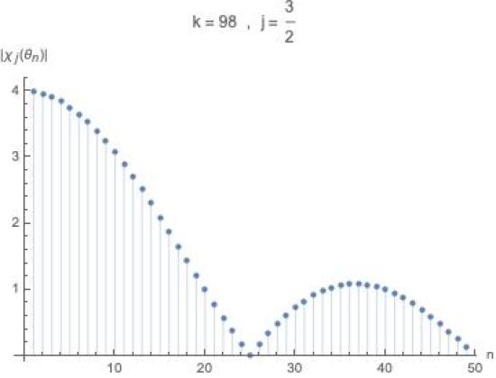
(a)

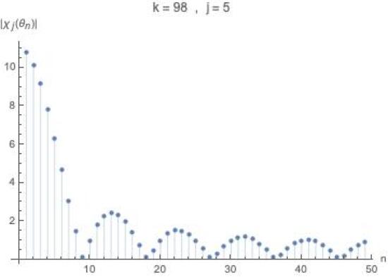
(b)

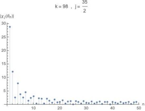
(c)

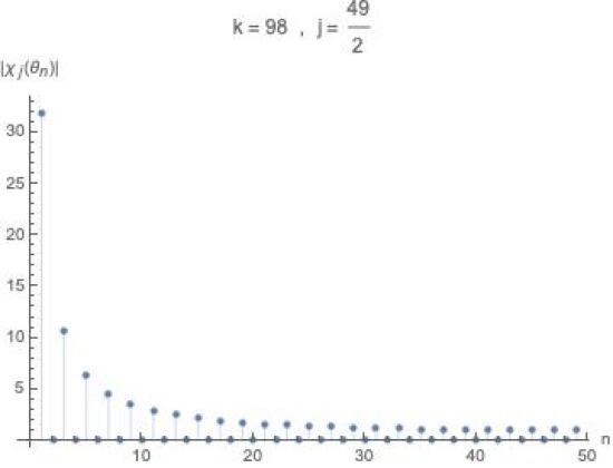
(d)

Figure 1: Figures (a),(b),(c) and (d) above show the variation with the discrete eigenvalue label $n$ of the absolute value of the character of four different integrable representations $|\chi_{j}(\theta_{n})|$ ($j=\frac{3}{2},5,\frac{35}{2},\frac{49}{2}$) for $k=98$.

Appendix H $q$-binomial identities

H.1 A ‘fermionic’ identity

In this appendix, we prove the following $q$-binomial identity

$$A_{N_{F},k_{F}}(x)\equiv\prod_{j=-(N_{F}-1)/2}^{(N_{F}-1)/2}(1+q^{j}x)=\sum_{n=0}^{N_{F}}\binom{N_{F}}{n}_{q}x^{n}\ .$$ (604)

This identity holds when $N_{F}$ is any integer, even or odd. In each case the product on the LHS is taken over the $N_{F}$ values for the variable $j$ given by

$$\Bigg{\{}-\frac{N_{F}-1}{2},\ -\frac{N_{F}-3}{2},\ \cdots,\ \frac{N_{F}-3}{2},\ \frac{N_{F}-1}{2}\Bigg{\}}\ .$$ (605)

Let us define the expression on the LHS of (604) as $f(x)$, i.e., we define

$$f(x)=\prod_{j=-(N_{F}-1)/2}^{(N_{F}-1)/2}(1+q^{j}x)\ .$$ (606)

It is then clear that

$$f(qx)=\prod_{j=-(N_{F}-1)/2}^{(N_{F}-1)/2}(1+q^{j+1}x)\ .$$ (607)

We use the relabelling $j+1=j^{\prime}$ to rewrite the RHS of (607) as

$$f(qx)=\prod_{j^{\prime}=-(N_{F}-3)/2}^{(N_{F}+1)/2}(1+q^{j^{\prime}}x)\ .$$ (608)

This can be written as

$$f(qx)=\frac{1+q^{(N_{F}+1)/2}x}{1+q^{-(N_{F}-1)/2}x}\prod_{j^{\prime}=-(N_{F}-1)/2}^{(N_{F}-1)/2}(1+q^{j^{\prime}}x)\ .$$ (609)

We thus see that

$$f(qx)=\frac{1+q^{(N_{F}+1)/2}x}{1+q^{-(N_{F}-1)/2}x}\ f(x)\ .$$ (610)

Alternatively, the above equation (610) can be rewritten as

$$\Big{(}1+q^{-(N_{F}-1)/2}x\Big{)}f(qx)=\Big{(}1+q^{(N_{F}+1)/2}x\Big{)}f(x)\ .$$ (611)

From the definition of the function $f(x)$ in (606), it is clear that it is a polynomial in $x$ of degree $N_{F}$. In other words, $f(x)$ can be written in the following general form

$$f(x)=\sum_{k=0}^{N_{F}}A_{k}x^{k}\ ,$$ (612)

where, $A_{k}$ is to be determined. It is also clear from the structure of the polynomial that $A_{0}=1$. Substituting (612) in (611), we see that

$$\Big{(}1+q^{-(N_{F}-1)/2}x\Big{)}\sum_{k=0}^{N_{F}}A_{k}q^{k}x^{k}=\Big{(}1+q^{(N_{F}+1)/2}x\Big{)}\sum_{k=0}^{N_{F}}A_{k}x^{k}\ .$$ (613)

Comparing the coefficients of the term $x^{k}$ from both sides, we get the following recursive relation for $k>0$,

$$A_{k}q^{k}+A_{k-1}q^{k-1}q^{-(N_{F}-1)/2}=A_{k}+A_{k-1}q^{(N_{F}+1)/2}\ .$$ (614)

Simplification of the above expression (614) gives

$$A_{k}=A_{k-1}\ \frac{q^{(N_{F}+1)/2}-q^{k}q^{-(N_{F}+1)/2}}{q^{k}-1}\ .$$ (615)

This can be written in a more symmetric form as below

$$A_{k}=A_{k-1}\ \frac{q^{(N_{F}+1-k)/2}-q^{-(N_{F}+1-k)/2}}{q^{k/2}-q^{-k/2}}\ .$$ (616)

In terms of $q$-numbers, (616) can be written as

$$A_{k}=A_{k-1}\ \frac{[N_{F}+1-k]_{q}}{[k]_{q}}\ ,$$ (617)

where recall that $[x]_{q}=\frac{q^{x/2}-q^{-x/2}}{q^{1/2}-q^{-1/2}}$. Applying the successive recursion relations, we get

$$A_{k}=A_{0}\ \frac{[N_{F}+1-k]_{q}[N_{F}+2-k]_{q}\cdots[N_{F}]_{q}}{[k]_{q}[k-1]_{q}\cdots[1]_{q}}\ .$$ (618)

The RHS of (618) can be rewritten in a simple way

$$A_{k}=A_{0}\frac{[N_{F}-k]_{q}![N_{F}+1-k]_{q}[N_{F}+2-k]_{q}\cdots[N_{F}]_{q}}{[k]_{q}!}\cdot\frac{1}{[N_{F}-k]_{q}!}\ .$$ (619)

which is nothing but

$$A_{k}=\frac{[N_{F}]_{q}!}{[k]_{q}![N_{F}-k]_{q}!}={N_{F}\choose k}_{q}\ .$$ (620)

where we have used $A_{0}=1$. This proves the identity (604).

H.2 A ‘bosonic’ identity

In this subsection, we prove the identity

$$B_{N_{B},k_{B}}(x)\equiv\prod_{j=-(N_{B}-1)/2}^{(N_{B}-1)/2}\frac{1}{(1-q^{j}x)}~{}\bigg{|}_{k_{B}}=\sum_{n=0}^{k_{B}}{N_{B}+n-1\choose n}_{q}x^{n}\ ,$$ (621)

where $q=\text{e}^{2\pi\text{i}/\kappa_{B}}$ where we have assumed that $N_{B}$ and $k_{B}$ are positive without loss of generality (for negative $k_{B}$, we replace $k_{B}\to|k_{B}|$ in all expressions below). The symbol $\big{|}_{k_{B}}$ tells us to expand the expression on the RHS in a power series in $x$ and truncate this expansion at order $k_{B}$. In this subsection, we will determine the expansion coefficients $B_{n}$ of the function

$$B_{N_{B},k_{B},\alpha}(x)\equiv\sum_{n=0}^{k_{B}}B_{n}x^{n}\ .$$ (622)

We will find it convenient to work with the function

$${g}(x)=\prod_{j=-(N_{B}-1)/2}^{(N_{B}-1)/2}\frac{1}{1-q^{j}x}\equiv\sum_{n=0}^{\infty}b_{n}x^{n}\ .$$ (623)

Clearly $=B_{n}=b_{n}$ for $n\leq k$, but $B_{n}=0$ for $n>k$. Knowledge of $b_{n}$ thus allows us to determine $B_{n}$.

We can find the quantities $b_{n}$ proceeding as in the previous subsection. The analog of (610) is

$$g(qx)=\frac{1-q^{-(N_{B}-1)/2}x}{1-q^{(N_{B}+1)/2}x}g(x)\ ,$$ (624)

or

$$\left(1-q^{(N_{B}+1)/2}x\right)g(qx)=\left(1-q^{-(N_{B}-1)/2}x\right)\ g(x)\ .$$ (625)

Plugging the series expansion (623) into (625) and equating powers of $x^{n}$ we find the recursion relation

$$b_{n}q^{n}-b_{n-1}q^{\frac{N_{B}+2n-1}{2}}=b_{n}-b_{n-1}q^{-\frac{N_{B}-1}{2}}\ .$$ (626)

Equivalently,

$$b_{n}=\frac{q^{\frac{N_{B}+n-1}{2}}-q^{-\frac{N_{B}+n-1}{2}}}{q^{\frac{n}{2}}-q^{-\frac{n}{2}}}\ b_{n-1}\ ,$$ (627)

that is,

$$b_{n}=\frac{[N_{B}+n-1]_{q}}{[n]_{q}}\ b_{n-1}\ .$$ (628)

The above equation holds for $n\geq 1$. Note that that $b_{0}=1$. It follows from (628) that

$$b_{n}=\prod_{k=1}^{n}\frac{[N_{B}+k-1]_{q}}{[k]_{q}}={N_{B}+n-1\choose n}_{q}\ .$$ (629)

and hence

$$B_{N_{B},k_{B}}(x)=\sum_{n=0}^{k_{B}}{N_{B}+n-1\choose n}_{q}x^{n}\ .$$ (630)

H.2.1 $b_{n}$ for $n>k_{B}$

Even though we do not need this for our paper, for completeness we study the structure of the quantity $b_{n}$ for $n>k_{B}$. The reader who is uninterested in this diversion should feel free to skip to the next subsection. In order to proceed, let us recall that when $q=\text{e}^{\frac{2\pi\text{i}}{\kappa_{B}}}$, we have

$$[m\,\kappa_{B}+a]_{q}=(-1)^{m}~{}[a]_{q}\ ,$$ (631)

for any integer $m$. In particular

$$[m\,\kappa_{B}]_{q}=0\ .$$ (632)

Notice that the numerator in the $q$-binomial coefficient (629) has a factor of $[\kappa_{B}]_{q}$ whereas the denominator has no such factor whenever $\kappa_{B}>n\geq k_{B}+1$. It follows that

$$b_{n}=0\quad{\rm for}\quad k_{B}+1\leq n\leq\kappa_{B}-1\ .$$ (633)

(compare with e.g. the discussion around (516)).

Moreover when $n=\kappa_{B}$, there is a factor of $[\kappa_{B}]$ in both the numerator and the denominator and hence $b_{\kappa_{B}}$ has a non-zero limiting value when we take $q\to\text{e}^{2\pi\text{i}/\kappa_{B}}$:

$$b_{\kappa_{B}} =\frac{\prod_{j=1}^{k_{B}}[N_{B}+j-1]_{q}\ [\kappa_{B}]_{q}\ \prod_{r=1}^{N_{B}-1}[\kappa_{B}+r]_{q}}{\prod_{s=1}^{\kappa_{B}}[s]_{q}}\ ,$$

$$=\frac{\prod_{j=1}^{k_{B}}[N_{B}+j-1]_{q}\ [\kappa_{B}]_{q}\ \prod_{r=1}^{N_{B}-1}(-[r]_{q})}{\prod_{s=1}^{\kappa_{B}}[s]_{q}}\ ,$$

$$=(-1)^{N_{B}-1}\frac{\prod_{j=1}^{k_{B}}[N_{B}+j-1]_{q}\ [\kappa_{B}]_{q}\ \prod_{r=1}^{N_{B}-1}[r]_{q}}{\prod_{s=1}^{\kappa_{B}}[s]_{q}}\ ,$$

$$=(-1)^{N_{B}-1}\frac{\prod_{j=1}^{\kappa_{B}}[j]_{q}}{\prod_{s=1}^{\kappa_{B}}[s]_{q}}=(-1)^{N_{B}-1}\ .$$ (634)

More generally, the reader can easily convince herself that for $j\leq 0<|\kappa_{B}|$

$$b_{m\kappa_{B}+j}=(-1)^{m(N_{B}-1)}\ b_{j}\ .$$ (635)

It then follows from (633) that

$$g(x) =\Big{(}1+(-1)^{N_{B}-1}x^{\kappa_{B}}+(-1)^{2(N_{B}-1)}x^{2\kappa_{B}}+\ldots\Big{)}\sum_{n=0}^{k_{B}}{N_{B}+n-1\choose n}_{q}x^{n}\ ,$$

$$=\frac{1}{1-(-1)^{N_{B}-1}x^{\kappa_{B}}}\sum_{n=0}^{k_{B}}{N_{B}+n-1\choose n}_{q}x^{n}\ .$$ (636)

In particular, when $N_{B}$ is odd we get

$$g(x)=\frac{1}{1-x^{\kappa_{B}}}\sum_{n=0}^{k_{B}}{N_{B}+n-1\choose n}_{q}x^{n}\ ,$$ (637)

whereas, when $N_{B}$ is even we get

$$g(x)=\frac{1}{1+x^{\kappa_{B}}}\sum_{n=0}^{k_{B}}{N_{B}+n-1\choose n}_{q}x^{n}\ .$$ (638)

H.3 A Bose-Fermi identity

In this subsection, $k_{B}$ and $k_{F}$ can have either sign. We demonstrate that the quantities $A_{N_{F},|k_{F}|}$ (604) and $B_{N_{B},|k_{B}|}$ (621) are equal to each other under the Bose-Fermi duality map $N_{B}=|k_{F}|$, $N_{F}=|k_{B}|$. That is,

$$B_{N_{B},|k_{B}|}(x)=A_{|k_{B}|,N_{B}}(x)\ ,$$ (639)

We reproduce the formulae for $A$ and $B$ below:

$$B_{N_{B},k_{B}}(x) \equiv\prod_{j=-(N_{B}-1)/2}^{(N_{B}-1)/2}\frac{1}{(1-q^{j}x)}~{}\bigg{|}_{k_{B}}=\sum_{n=0}^{k_{B}}{N_{B}+n-1\choose n}_{q}x^{n}\ ,$$

$$A_{N_{F},k_{F}}(x) \equiv\prod_{j=-(N_{F}-1)/2}^{(N_{F}-1)/2}(1+q^{j}x)=\sum_{n=0}^{N_{F}}{N_{F}\choose n}_{q}x^{n}\ .$$ (640)

We show (639) in two ways. First, we show that the following $q$-combinatorial identity holds:

$$\binom{k}{n}_{q}=\binom{N+n-1}{n}_{q}\ ,$$ (641)

for any two positive integers $k$ and $N$ which satisfy $k+N=\kappa$ with $q=\text{e}^{2\pi\text{i}/\kappa}$.

We have, by definition,

$${k\choose n}_{q}=\frac{[k]_{q}!}{[n]_{q}![k-n]_{q}!}=\frac{[k]_{q}[k-1]_{q}\cdots[k-n+1]_{q}}{[n]_{q}!}\ .$$ (642)

Using $q=\text{e}^{2\pi\text{i}/\kappa}$ and $k+N=\kappa$, it is not hard to see that

$$[k-i]_{q}=[N+i]_{q}\ ,\quad\text{for every}\quad i=0,\ldots,k\ ,$$ (643)

which gives

$${k\choose n}_{q}=\frac{[N]_{q}[N+1]_{q}\cdots[N+n-1]_{q}}{[n]_{q}!}=\binom{N+n-1}{n}_{q}\ .$$ (644)

Since $\kappa=N_{B}+|k_{B}|=N_{F}+|k_{F}|$, the Bose-Fermi duality map then gives

$$\binom{N_{F}}{n}_{q}=\binom{|k_{B}|}{n}_{q}=\binom{N_{B}+n-1}{n}_{q}\ ,$$ (645)

from which (639) follows.

The second proof of (639) uses the product form of $A$ and $B$. It is convenient to present the proof separately for four cases.

H.3.1 $N_{B}$ odd

In this case, the product in the expression for $B$ (H.3) is taken over the $N_{B}$ values of $q^{j}$ that are $\kappa^{\rm th}$ roots of unity. To process that formula we multiply both the numerator and the denominator by $\prod_{q^{\prime}}(1-q^{\prime}x)$ where $q^{\prime}$ run over the remaining $|k_{B}|$ $\kappa^{\rm th}$ roots of unity:

$$B_{N_{B},|k_{B}|}(x)=\left[\prod_{q^{\prime}}(1-q^{\prime}x)\prod_{j=0}^{\kappa-1}(1-q^{j}x)^{-1}\right]_{|k_{B}|}\ ,$$ (646)

Now, when $k_{B}$ is odd, then $\kappa=N_{B}+|k_{B}|$ is an even integer. This implies that $-q^{\prime}$ is also a $\kappa^{\rm th}$ root of unity. Relabelling $q^{\prime}$ as $-q^{\prime}$ in the numerator gives a product over $|k_{B}|$ $\kappa^{\rm th}$ roots of $-1$. When $k_{B}$ is an even integer, $\kappa$ is an odd integer. Then $-q^{\prime}$ is a $\kappa^{\rm th}$ root of $-1$ rather than of unity. Relabelling $q^{\prime}\to-q^{\prime}$ now gives a product over $|k_{B}|$ $\kappa^{\rm th}$ roots of $-1$ in the numerator. Thus, for either $|k_{B}|$ even or odd, we can write

$$B_{N_{B},|k_{B}|}(x) =\left[\prod_{q^{\prime}}(1+q^{\prime}x)\prod_{j=0}^{\kappa-1}(1-q^{j}x)^{-1}\right]_{|k_{B}|}\ ,$$

$$=\left[\prod_{j=-(|k_{B}|-1)/2}^{(|k_{B}|-1)/2}(1+q^{j}x)\prod_{j=0}^{\kappa-1}(1-q^{j}x)^{-1}\right]_{|k_{B}|}\ ,$$ (647)

where one can indeed check that the product in the numerator is a product over $|k_{B}|$ $\kappa^{\rm th}$ roots of unity when $k_{B}$ is odd and $\kappa^{\rm th}$ roots of $-1$ when $k_{B}$ is even. Next, using the identity

$$\prod_{j=0}^{\kappa-1}(1-q^{j}x)=1-x^{\kappa}\ ,$$ (648)

we find that (646) simplifies to

$$B_{N_{B},|k_{B}|}(x)=\left[\prod_{j=-(|k_{B}|-1)/2}^{(|k_{B}|-1)/2}(1+q^{j}x)(1-x^{\kappa})^{-1}\right]_{|k_{B}|}\ .$$ (649)

As in the discussion around (103), the denominator in (649) admits a power series expansion in $x^{\kappa}$; none of the non-trivial terms in this expansion contribute once we truncate the expansion at order $|k_{B}|$ and so the denominator can simply be replaced by unity. On the other hand the numerator is already a polynomial of degree $|k_{B}|$. It follows that (649) further simplifies to

$$B_{N_{B},|k_{B}|}(x)=\prod_{j=-(|k_{B}|-1)/2}^{(|k_{B}|-1)/2}(1+q^{j}x)\ ,$$ (650)

which, upon using $|k_{B}|=N_{F}$ gives the product form for $A$ in (H.3).

H.3.2 $N_{B}$ even

In this case the product for $B$ in (H.3) is taken over $N_{B}$ values of $q^{j}$ which are all $\kappa^{\rm th}$ roots of $-1$. As in the previous subsubsection we multiply both the numerator and the denominator by $\prod_{q^{\prime}}(1-q^{\prime}x)$ where $q^{\prime}$ run over the remaining $|k_{B}|$ $\kappa^{\rm th}$ roots of $-1$ to get

$$B_{N_{B},|k_{B}|}(x)=\left[\prod_{q^{\prime}}(1-q^{\prime}x)\prod_{j=0}^{\kappa-1}(1-q^{j+\frac{1}{2}}x)^{-1}\right]_{|k_{B}|}\ ,$$ (651)

When $k_{B}$ is an odd integer, $\kappa=N_{B}+|k_{B}|$ is an odd integer. Thus, $-q^{\prime}$ is a $\kappa^{\rm th}$ root of unity rather than of $-1$. When $k_{B}$ is even, $\kappa$ is even and $-q^{\prime}$ is also a $\kappa^{\rm th}$ root of $-1$. Relabelling $q^{\prime}\to-q^{\prime}$ in the numerator, we get a product over $|k_{B}|$ $\kappa^{\rm th}$ roots of unity when $k_{B}$ is odd and $\kappa^{\rm th}$ roots of $-1$ when $k_{B}$ is even. In either case, we can write

$$B_{N_{B},|k_{B}|}(x)=\left[\prod_{j=-(|k_{B}|-1)/2}^{(|k_{B}|-1)/2}(1+q^{j}x)\prod_{j=0}^{\kappa-1}(1-q^{j+\frac{1}{2}}x)^{-1}\right]_{|k_{B}|}\ ,$$ (652)

Next, using the identity

$${\prod_{j=0}^{\kappa-1}(1-q^{j+\frac{1}{2}}x)}=1+x^{\kappa}\ ,$$ (653)

we find that (652) simplifies to

$$B_{N_{B},|k_{B}|}(x)=\left[\prod_{j=-(|k_{B}|-1)/2}^{(|k_{B}|-1)/2}(1+q^{j}x)(1+x^{\kappa})^{-1}\right]_{|k_{B}|}\ .$$ (654)

As in the previous case the truncation to order $|k_{B}|$ allows us to discard the contributions from $(1+x^{\kappa})^{-1}$ and simplify (652) to

$$B_{N_{B},|k_{B}|}(x)=\ \prod_{j=-(|k_{B}|-1)/2}^{(|k_{B}|-1)/2}(1+q^{j}x^{\prime})\ .$$ (655)

Plugging in $|k_{B}|=N_{F}$ once again yields (639).

Appendix I Entropy as a function of occupation numbers

I.1 Entropy as a function of occupation number for free fermions

In the limit $k_{F}\to\infty$, the partition function of any number of fundamental particles occupying the state with energy $E_{a}$ is given by

$$\mathfrak{z}_{F}(y_{a})=\sum_{n=0}^{N_{F}}{N_{F}\choose n}y_{a}^{n}=(1+y_{a})^{N_{F}}\ ,$$ (656)

with $y_{a}=\text{e}^{-\beta(E_{a}-\mu)}$. The average occupation number of this state is given by

$$n_{a}=\frac{\sum_{n=0}^{N_{F}}ny_{a}^{n}~{}{N_{F}\choose n}}{\mathfrak{z}_{F}}=y_{a}\partial_{y_{a}}\log\mathfrak{z}_{F}=\frac{N_{F}}{y_{a}^{-1}+1}\ .$$ (657)

The entropy is then determined by (6.1) i.e.

$$S_{F}=-n_{a}(y_{a})\log y_{a}+\log\mathfrak{z}_{F}(y_{a})\ .$$ (658)

Inverting (657) to solve for $y_{a}$ in favour of $n_{a}$ we find

$$\frac{1}{y_{a}}=\frac{N_{F}}{n_{a}}-1\ .$$ (659)

Substituting (659) into (656) and (658), we find

$$S_{F}(n_{a}) =n_{a}\log\left(\frac{N_{F}-n_{a}}{n_{a}}\right)+N_{F}\log\left(\frac{N_{F}}{N_{F}-n_{a}}\right)\ ,$$

$$=-(N_{F}-n_{a})\log(N_{F}-n_{a})-n_{a}\log n_{a}+N_{F}\log N_{F}\ .$$ (660)

In (I.1) we have succeeded in rewriting the entropy of this single state as a function of its occupation number. It is now easy to take the derivative of the entropy with respect to $n_{a}$; we find

$$\partial_{n_{a}}S_{F}(n_{a})=\log\left(\frac{N_{F}-n_{a}}{n_{a}}\right)\ .$$ (661)

As explained in Section 6.3, we can now extremize the entropy of our system at fixed energy and charge. The quantity defined in (207), i.e.

$$\sum_{a}(S_{F}(n_{a})-\beta E_{a}n_{a}+\beta\mu n_{a})\ ,$$ (662)

is now an explicit function of $n_{a}$. Extremizing with respect to $n_{a}$ we find

$$\log\left(\frac{N_{F}-n_{a}}{n_{a}}\right)-\beta E_{a}+\beta\mu=0\ .$$ (663)

Solving (663) for $n_{a}$ we obtain

$$n_{a}=\frac{N_{F}}{\text{e}^{\beta(E_{a}-\mu)}+1}\ ,$$ (664)

in agreement with (657).

I.2 Entropy as a function of occupation number for free bosons

In the case of free bosons, the single-state partition function of any number of fundamental bosons occupying a single-particle state of energy $E_{a}$ at finite chemical potential $\mu$, is given by

$$\mathfrak{z}_{B}(y_{a})=\sum_{n=0}^{\infty}\ {N_{B}+n-1\choose n}\ y_{a}^{n}=\frac{1}{(1-y_{a})^{N_{B}}}\ ,$$ (665)

where $y_{a}=\text{e}^{-\beta(E_{a}-\mu)}$. The occupation number in this state is given by

$$n_{a}=\frac{1}{\mathfrak{z}_{B}(y_{a})}\sum_{n=0}^{\infty}\ {N_{B}+n-1\choose n}\ ny_{a}^{n}=y_{a}\partial_{y_{a}}\log\mathfrak{z}_{B}=\frac{N_{B}}{y_{a}^{-1}-1}\ .$$ (666)

It is easy to invert the final expression of (666) to write $y_{a}$ as a function of $n_{a}$ as below

$${y_{a}}=\frac{n_{a}}{N_{B}+n_{a}}\ .$$ (667)

We now set to compute the entropy of this single energy state by using the expression (658). Inserting $y_{a}$ as a function of $n_{a}$ in (658), we get

$$S_{B}(n_{a}) =-n_{a}\log\left(\frac{n_{a}}{N_{B}+n_{a}}\right)-N_{B}\log\left(\frac{N_{B}}{N_{B}+n_{a}}\right)$$ (668)

$$=-n_{a}\log n_{a}+(N_{B}+n_{a})\log(N_{B}+n_{a})-N_{B}\log N_{B}\ .$$ (669)

I.3 Explicit expressions in the large volume, large $N$ ’t Hooft limit

I.3.1 For fermions

In this section, we study the problem of determining the entropy as a function of occupation numbers for fermions in the large $N_{F}$ ’t Hooft limit. Recall the formulae for the occupation numbers (4.4) in the large volume limit,

$$n_{F}(y) =\sum_{j=-(N_{F}-1)/2}^{(N_{F}-1)/2}\frac{1}{y^{-1}q^{-j}+1}\ ,$$

$$n_{B}(y) =\left(\sum_{j=-(N_{B}-1)/2}^{(N_{B}-1)/2}\frac{1}{y^{-1}q^{-j}-1}\right)-\frac{|\kappa_{B}|}{1-y^{-|\kappa_{B}|}(-1)^{N_{B}-1}}\ ,$$ (670)

In the large $N$ limit, it is convenient to define the occupation number per colour

$$\bar{n}_{F}=\frac{n_{a}}{N_{F}}\ .$$ (671)

At leading order in the large $N_{F}$ limit, the summation in (I.3.1) turns into an integral, and we find (see Eq 5.6 of Minwalla:2020ysu )

$$\bar{n}_{F}(y)=\frac{1}{2}-\frac{1}{\pi|{\lambda}_{F}|}\tan^{-1}\Big{(}\frac{1-y}{1+y}\tan\frac{\pi|{\lambda}_{F}|}{2}\Big{)}\ .$$ (672)

This expression is easily inverted; making the $\tan^{-1}$ the ‘subject of the formula’ and taking the tan of both sides give

$$\frac{1-y}{1+y}=\frac{\tan\big{(}\frac{\pi|\lambda_{F}|}{2}(1-2\bar{n}_{F})\big{)}}{\tan\big{(}\frac{\pi|{\lambda_{F}}|}{2}\big{)}}\ .$$ (673)

Using (673) it is easy to solve for $y$ in terms of ${\bar{n}}_{F}$. Simplifying the resultant expression we find

$$y=\frac{\sin\big{(}\pi|{\lambda}_{F}|\bar{n}_{F}\big{)}}{\sin\big{(}\pi|{\lambda}_{F}|(1-\bar{n}_{F})\big{)}}=\frac{[n_{F}]_{q}}{[N_{F}-n_{F}]_{q}}\ .$$ (674)

Using the equation $n_{a}=y_{a}\partial_{y_{a}}\log\mathfrak{z}_{F}(y_{a})$, we find

$$\log\mathfrak{z}_{F}(y)=N_{F}\int\bar{n}_{F}\ \frac{dy}{y}\ .$$ (675)

It follows from (674) that

$$\frac{dy}{y}=\pi|\lambda_{F}|\Big{(}\cot\big{(}\pi|\lambda_{F}|\bar{n}_{F}\big{)}+\cot\big{(}\pi|\lambda_{F}|(1-\bar{n}_{F})\big{)}\Big{)}\ d\bar{n}_{F}\ .$$ (676)

Substituting (676) into (675) and integrating with respect to ${\bar{n}}_{F}$ we find

$$\log\mathfrak{z}_{F}=N_{F}\pi|\lambda_{F}|\int\bar{n}_{F}\ \Big{(}\cot\big{(}\pi|\lambda_{F}|\bar{n}_{F}\big{)}+\cot\big{(}\pi|\lambda_{F}|(1-\bar{n}_{F})\big{)}\Big{)}\ d\bar{n}_{F}\ .$$ (677)

Similarly, using (199) for the entropy i.e.

$$\partial_{n}S=-\log y\ ,$$ (678)

and using (674), we get

$$S_{F}=-\int^{{n}_{a}}_{0}\bigg{(}\log\big{(}[n^{\prime}_{a}]_{q}\big{)}-\log\big{(}[N_{F}-n^{\prime}_{a}]_{q}\big{)}\bigg{)}\ d{n}^{\prime}_{a}\ .$$ (679)

We could have gotten the above result (679) by using (658) and the expression (677) for $\log\mathfrak{z}_{F}$. Indeed, performing the integral in (677) (and fixing the integration constant using the condition that the entropy vanishes when $n_{a}$ vanishes) we find

$$S_{F} =-N_{F}\Bigg{[}\bar{n}_{F}\log\frac{\sin\big{(}\pi|\lambda_{F}|\bar{n}_{F}\big{)}}{\sin\big{(}\pi|\lambda_{F}|(1-\bar{n}_{F})\big{)}}$$

$$\qquad-\pi|\lambda_{F}|\int^{\bar{n}_{F}}_{0}\bar{n}^{\prime}_{F}\ \Big{(}\cot\big{(}\pi|\lambda_{F}|\bar{n}^{\prime}_{F}\big{)}+\cot\big{(}\pi|\lambda_{F}|(1-\bar{n}^{\prime}_{F})\big{)}\Big{)}\ d\bar{n}^{\prime}_{F}\Bigg{]}\ .$$ (680)

The expression on the RHS of (I.3.1) can be manipulated as follows. Performing integration by parts in the second line of the above integral, (I.3.1) can be rewritten as

$$S_{F} =-N_{F}\Bigg{[}\bar{n}_{F}\log\frac{\sin\big{(}\pi|\lambda_{F}|\bar{n}_{F}\big{)}}{\sin\big{(}\pi|\lambda_{F}|(1-\bar{n}_{F})\big{)}}$$

$$\qquad-\bar{n}_{F}\ \Big{(}\log\sin\big{(}\pi|\lambda_{F}|\bar{n}_{F}\big{)}-\log\sin\big{(}\pi|\lambda_{F}|(1-\bar{n}_{F})\big{)}\Big{)}$$ (681)

$$\qquad+\int^{\bar{n}_{F}}_{0}\Big{(}\log\sin\big{(}\pi|\lambda_{F}|\bar{n}^{\prime}_{F}\big{)}-\log\sin\big{(}\pi|\lambda_{F}|(1-\bar{n}^{\prime}_{F})\big{)}\Big{)}\ d\bar{n}^{\prime}_{F}\Bigg{]}\ .$$ (682)

The terms on the first and second line on the RHS of the above expression (I.3.1) cancel each other so (I.3.1) takes the simplified form

$$S_{F} =-N_{F}\int^{\bar{n}_{F}}_{0}\Big{(}\log\sin\big{(}\pi|\lambda_{F}|\bar{n}^{\prime}_{F}\big{)}-\log\sin\big{(}\pi|\lambda_{F}|(1-\bar{n}^{\prime}_{F})\big{)}\Big{)}\ d\bar{n}^{\prime}_{F}\ ,$$

$$=-\int^{{n}_{a}}_{0}\bigg{(}\log\sin\Big{(}\frac{\pi}{|\kappa_{F}|}{n}^{\prime}_{a}\Big{)}-\log\sin\Big{(}\frac{\pi}{|\kappa_{F}|}(N_{F}-{n}^{\prime}_{a})\Big{)}\bigg{)}\ d{n}^{\prime}_{a}\ ,$$

$$=-\int^{{n}_{a}}_{0}\bigg{(}\log\big{(}[n^{\prime}_{a}]_{q}\big{)}-\log\big{(}[N_{F}-n^{\prime}_{a}]_{q}\big{)}\bigg{)}\ d{n}^{\prime}_{a}\ .$$ (683)

As a check on the formula (679) we note that in the limit $\lambda_{F}\to 0$, (679) gives

$$S_{F}=-N_{F}\bigg{(}\bar{n}_{F}\log\bar{n}_{F}+(1-\bar{n}_{F})\log(1-\bar{n}_{F})\bigg{)}\ ,$$ (684)

in perfect agreement with (I.1).

I.3.2 For bosons

We repeat the analysis of the previous subsubsection I.3.1 here in the case of bosons. As in the case of fermions, it is useful to define the average occupation number for bosons as

$$\bar{n}_{B}=\frac{n_{a}}{N_{B}}\ .$$ (685)

In the strict large $N_{B}$ limit, the average occupation number has been worked out in detail in Minwalla:2020ysu (see Eq $5.21$ of Minwalla:2020ysu ). It is given by

$$\bar{n}_{B}=\frac{1-|\lambda_{B}|}{2|\lambda_{B}|}-\frac{1}{\pi|\lambda_{B}|}\tan^{-1}\bigg{(}\frac{1-y}{1+y}\cot\frac{\pi|\lambda_{B}|}{2}\bigg{)}\ .$$ (686)

It is useful to invert the above expression (686) to write $y$ as a function of $\bar{n}_{B}$. Inverting (686), we get

$$\frac{1-y}{1+y}=\frac{\cot\Big{(}\frac{\pi|\lambda_{B}|}{2}(1+2\bar{n}_{B})\Big{)}}{\cot\Big{(}\frac{\pi|\lambda_{B}|}{2}\Big{)}}\ .$$ (687)

Further simplification of (687) gives

$$y=\frac{\sin\big{(}\pi|\lambda_{B}|\bar{n}_{B}\big{)}}{\sin\big{(}\pi|\lambda_{B}|(1+\bar{n}_{B})\big{)}}=\frac{[n_{B}]_{q}}{[n_{B}+N_{B}]_{q}}\ .$$ (688)

The entropy can again be obtained by (678) and is given by

$$S_{B}=-\int^{{n}_{a}}_{0}\bigg{(}\log\big{(}[n^{\prime}_{a}]_{q}\big{)}-\log\big{(}[N_{B}+n^{\prime}_{a}]_{q}\big{)}\bigg{)}\ d{n}^{\prime}_{a}\ .$$ (689)

As a check on the formula (689) we note that in the limit $\lambda_{B}\to 0$, (689) gives

$$S_{B} =N_{B}\Bigg{(}-\bar{n}_{B}\log\bar{n}_{B}+(1+\bar{n}_{B})\log(1+\bar{n}_{B})\bigg{)}\ ,$$

$$=-n_{a}\log n_{a}+(N_{B}+n_{a})\log(N_{B}+n_{a})-N_{B}\log N_{B}\ ,$$ (690)

in perfect agreement with (668).

Appendix J One-loop determinants in $U(N)_{k,k^{\prime}}$ Chern-Simons theories

Following Blau and Thompson Blau:1993tv (see also Section 4.1 of Jain:2013py ) one may evaluate the path integral of pure Chern-Simons theories on $\Sigma_{g}\times S^{1}$ as follows. Denote the components of the gauge field along the two dimensional surface $\Sigma$ as $A_{\alpha}$, $\alpha=1,2$, and the time component as $A_{0}$, and make the following choice of gauge:

• We demand $\partial_{0}A_{0}=0$. This choice leaves time independent- so effectively two-dimensional - $U(N)$ gauge transformations unfixed.

• $A_{0}$ (which is now constant in time) is then chosen to be a diagonal matrix at each point on $\Sigma_{g}$. This choice is similar to one adopted by ’t Hooft in his classic studies of confinement in gauge theories, but this time in two rather than four spacetime dimensions.

The gauge invariance which is not fixed by (1) and (2) are diagonal gauge transformations that are constant in time, corresponding to a $U(1)^{N}$ gauge group in two dimensions. These affect only the constant mode along $S^{1}$ of the gauge field $A_{\alpha}$ along $\Sigma_{g}$, which we label $\mathring{A}_{\alpha}$. Further, only the diagonal components of $\mathring{A}_{\alpha}$ transform as gauge fields of the $U(1)^{N}$ whereas the off-diagonal components transform in the ‘adjoint representation’ of $U(1)^{N}$ i.e. the $ij^{\rm th}$ off-diagonal element $(\mathring{A}_{\alpha})_{ij}$ transforms with charge $-1$ under the $i^{\rm th}$ $U(1)$ and with charge $+1$ under the $j^{\rm th}$ $U(1)$.

• The $U(1)^{N}$ abelian gauge invariance can be fixed by imposing the Coulomb gauge on the diagonal components of $\mathring{A}_{\alpha}$: $\partial_{\alpha}\mathring{A}^{\textbf{t}}_{\alpha}=0$. We have now completely fixed (small) gauge invariance.

The gauge choices (1), (2) and (3) above leaves us with the path integral over a gauge-fixed abelian two dimensional theory. The gauge fixing procedure has singularities when two eigenvalues collide; as explained in detail in section 4.1 of Jain:2013py , these singularities are codimension 1 in field space and divide field space into sectors. From the point of view of the resultant 2 dimensional abelian theory, the different sectors correspond to working with different flux backgrounds. In other words the net effect of the ’t Hooftian singularities in field space is to force us to sum over (correctly quantized) $U(1)^{N}$ fluxes. The summation over these flux sectors played a central role in Sections 7.3.7 and 7.4.8. In particular the summation over $m_{i}$ (294) is the summation over these fluxes, while the term $w_{i}^{-\kappa m_{i}-s\sum_{j}m_{j}}$ in the same equation is the classical Chern-Simons action (in the dimensional regulation scheme) of a configuration that contains both flux and nonzero holonomies. In this Appendix we will explain that the remaining terms in (294), namely

$$\prod_{i<j}|w_{i}-w_{j}|^{2-2g}\times(-1)^{(N-1)\sum_{i}m_{i}}\ ,$$ (691)

make up the one-loop contribution to the Chern-Simons partition function evaluated in a given flux sector.

To proceed it is useful to define some notation. We use the superscript ${\bf t}$ to denote a matrix that is purely diagonal whereas a superscript ${\bf k}$ denotes a matrix that is purely off diagonal. The $\delta$ function that implements the first two gauge conditions (i.e. all but the Coulomb gauge fixing) is given by

$$\int[dB]\exp\left(\text{i}\int d^{3}x\,\text{Tr}(BA_{0})\right)\ ,$$ (692)

where $B=B^{\textbf{t}}+B^{\textbf{k}}$ is an adjoint-valued bosonic Lagrange multiplier constrained so that the constant (on the $S^{1}$) part of $B^{\bf t}$ vanishes. This constraint is needed to ensure that $B$ actually implements the first two gauge conditions above rather than simply setting all of $A_{0}$ to zero. The Faddeev-Popov determinant associated with the first two gauge conditions above is generated by the path integral

$$\int[dcd\bar{c}]\,\exp\left(\text{i}\int d^{3}x\,\text{Tr}\left(\bar{c}D_{0}c\right)\right)\ ,$$ (693)

where $c$ and ${\bar{c}}$ are fermionic $U(N)$ matrices such that the zero mode (on $S^{1}$) of $c^{\bf t}$ and $\bar{c}^{\textbf{t}}$ are constrained to vanish. Completely explicitly our path integral is generated by the effective action

$$\mathcal{S}_{\rm CS}[A,c,\bar{c},B]=\frac{\text{i}k}{2\pi}\int_{\Sigma\times S^{1}}dt\,\text{Tr}\left(A_{0}^{\textbf{t}}dA^{\textbf{t}}+A^{\textbf{t}}\partial_{0}A^{\textbf{t}}+A^{\textbf{k}}D_{0}A^{\textbf{k}}\right)\\ +\frac{\text{i}(s+1)}{2\pi}\int_{\Sigma\times S^{1}}dt\,\left(\text{Tr}(A_{0}^{\textbf{t}})d\text{Tr}(A^{\textbf{t}})+\text{Tr}(A^{\textbf{t}})\partial_{0}\text{Tr}(A^{\textbf{t}})\right)\\ +\text{i}\int d^{3}x\,\text{Tr}(BA_{0})+\text{i}\int d^{3}x\,\text{Tr}\left(\bar{c}^{\textbf{k}}D_{0}c^{\textbf{k}}+\bar{c}^{\textbf{t}}\partial_{0}c^{\textbf{t}}\right)\ ,$$ (694)

and also includes the delta function that imposes the $U(1)^{N}$ Coulomb gauge condition.

The zero mode (on $S^{1}$) of $A^{\bf t}$ contributes only to the first terms on the first and second lines of (694). As explained under equation 4.4 in Jain:2013py , the integral over the zero modes of $A^{\bf t}$ yields a delta function that forces $\nabla^{2}A^{\textbf{t}}_{0}$ to vanish on the $S^{2}$ and consequently forces $A^{\textbf{t}}_{0}$ to be a constant on the $S^{2}$. Invariance under large gauge transformations i.e. gauge transformations which are constant on $S^{2}$ but not connected to identity, forces $A^{\textbf{t}}_{0}$ to be periodic so that the holonomy $U=\text{e}^{\text{i}\beta A^{\textbf{t}}_{0}}$ is the only physical variable.

It now remains to perform the path integral over $c$ and ${\bar{c}}$, as well as the integral over $A$. This path integral is quadratic and so yields the ratio of determinants

$$\frac{\text{det}_{S}(D_{0})}{\sqrt{\text{det}_{V}(D_{0})}}\ ,$$ (695)

where the numerator of this expression is the Faddeev-Popov determinant and the denominator is the path integral over the gauge fields $A$, omitting the zero modes (on $S^{1}$) of the diagonal parts of $A$ since have already been integrated out (recall that they were responsible for setting $A^{\textbf{t}}_{0}$ to be constant on $S^{2}$).

As the operator $D_{0}$ has no spatial derivatives, the determinants in both the numerator and denominator are highly divergent. At least roughly, however, it is not difficult to convince oneself that these divergences cancel between the numerator and denominator. A rough (and as we will see below, importantly inaccurate) evaluation of the ratio of determinants proceeds as follows (see Section 4.4 of Jain:2013py ). Any vector field on a genus $g$ surface $\Sigma_{g}$ is a linear combination over the $2g$ nontrivial harmonic vector fields plus the gradient of a scalar $\phi$ plus the Hodge dual of the gradient of a second scalar $\chi$. The zero modes (on $\Sigma_{g}$) of the scalar fields $\chi$ and $\phi$ do not appear in the formula for $A$ and so should be omitted in this construction. The contribution to the determinant from the non-zero modes of $\phi$ and $\chi$ cancel the part of the determinant in the numerator that comes from the non-zero modes (on $\Sigma_{g}$) of the ghosts. Of course we should really proceed by carefully regulating both determinants before cancelling. Boldly (and unwisely) ignoring such subtleties, we find that the numerator receives contributions only from zero modes on $\Sigma_{g}$ (but from all modes along $S^{1}$) and so evaluates to

$$\prod_{1\leq i<j\leq N}|w_{i}-w_{j}|^{2}\ .$$ (696)

On the other hand the denominator receives contributions only from the coefficients of the $2g$ nontrivial harmonic vector fields, one factor of (696) from each. Including the square root, the contribution from the gauge field is

$$\frac{1}{\prod_{1\leq i<j\leq N}|w_{i}-w_{j}|^{2g}}.$$

Putting the contributions of the numerator and denominator together, we obtain

$$\prod_{1\leq i<j\leq N}|w_{i}-w_{j}|^{2-2g}\ ,$$ (697)

in partial agreement with (691).

The arguments of the previous paragraph were crude, and indeed turn out not to be completely precise. Happily, Blau and Thompson have evaluated the ratio of determinants (695) much more carefully. The result they obtain using a heat-kernel regularization scheme is Blau:1993tv

$$\frac{\text{det}_{S}(D_{0})}{\sqrt{\text{det}_{V}(D_{0})}}\ =\prod_{\alpha\in\Delta_{+}}\exp\left(\frac{1}{8\pi}\int_{\Sigma_{g}}R\log(M_{\alpha}M_{-\alpha})-\frac{1}{2\pi}\int_{\Sigma}\alpha_{i}F_{i}\log\frac{M_{\alpha}}{M_{-\alpha}}\right)\ ,$$ (698)

Here $\alpha$ runs over the set of positive roots $\Delta_{+}$ of $SU(N)$, $R$ is the scalar curvature of $\Sigma_{g}$, $F_{i}$ is the $i^{\rm th}$ component on the diagonal of the gauge field strength along $\Sigma_{g}$ and

$$M_{\alpha}=1-\text{e}^{\text{i}\alpha^{i}\phi_{i}}\ ,$$ (699)

where $\phi=\{\phi_{1},\ldots,\phi_{N}\}$ are the compact diagonal elements of $A^{\textbf{t}}_{0}$ and $\alpha^{i}$ is the $i^{\rm th}$ component of the root $\alpha$. Let us write the above product explicitly for $U(N)$. As discussed in Sections 7.3.2, 7.4.1, the positive roots for $SU(N)$ (and $U(N)$) are written in terms of the orthonormal basis as

$$\alpha_{ij}=\epsilon_{i}-\epsilon_{j}\ ,\quad 1\leq i<j\leq N\ .$$ (700)

This gives

$$M_{\alpha_{(ij)}}=1-\text{e}^{\text{i}(\phi_{i}-\phi_{j})}\ .$$ (701)

Note that $\phi_{i}$ is a constant along $\Sigma_{g}$ due to integrating out the fluctuating part of the abelian gauge field $A^{\textbf{t}}$ along $\Sigma_{g}$. Using $\frac{1}{4\pi}\int_{\Sigma_{g}}d^{2}zR=2-2g$, the first term in the above exponential gives the usual Vandermonde factor raised to $1-g$:

$$\prod_{1\leq i<j\leq N}\left[(1-\text{e}^{\text{i}(\phi_{i}-\phi_{j})})(1-\text{e}^{-\text{i}(\phi_{i}-\phi_{j})})\right]^{1-g}=\prod_{1\leq i<j\leq N}|\text{e}^{\text{i}\phi_{i}}-\text{e}^{\text{i}\phi_{j}}|^{2-2g}\ .$$ (702)

Let us next focus on the second factor. We have

$$\exp\left(-\sum_{\alpha\in\Delta_{+}}\frac{1}{2\pi}\int_{\Sigma_{g}}\alpha_{i}F_{i}\log(-\text{e}^{\text{i}\alpha_{i}\phi_{i}})\right)\\ =\exp\left(-\frac{1}{2\pi}\int_{\Sigma_{g}}2\rho_{i}F_{i}\log(-1)\right)\exp\left(-\sum_{\alpha\in\Delta_{+}}\frac{\text{i}}{2\pi}\int_{\Sigma_{g}}(\alpha_{i}F_{i})(\alpha_{j}\phi_{j})\right)\ ,$$ (703)

where $\rho=\tfrac{1}{2}\sum_{\alpha\in\Delta_{+}}\alpha$ is the Weyl vector. The integral of the field strength $F_{i}$ over $\Sigma$ is $2\pi m_{i}$ where $m_{i}$ is an integer. Substituting this, we get

$$\exp\left(-2\rho_{i}m_{i}\log(-1)\right)\exp\left(-\text{i}\sum_{\alpha\in\Delta_{+}}(\alpha_{i}m_{i})(\alpha_{j}\phi_{j})\right)\ .$$ (704)

The expression in (704) is a product of two terms. Let us first study the second of these, namely

$$\exp\left(-\text{i}\sum_{\alpha\in\Delta_{+}}(\alpha_{i}m_{i})(\alpha_{j}\phi_{j})\right).$$

Following Blau:1993tv we now explain that this term effectively implements the shift $k\rightarrow\kappa$. Writing the sum over $\alpha\in\Delta_{+}$ explicitly, we have

$$\exp\left(-\text{i}\sum_{\alpha\in\Delta_{+}}(\alpha_{i}m_{i})(\alpha_{j}\phi_{j})\right)=\exp\left(-\text{i}\sum_{1\leq i<j\leq N}(\alpha_{(ij)})_{p}m_{p}\,(\alpha_{(ij)})_{u}\phi_{u}\ \right),$$

$$\quad=\exp\left(-\text{i}\sum_{1\leq i<j\leq N}(m_{i}-m_{j})(\phi_{i}-\phi_{j})\right)=\exp\left(-\frac{\text{i}}{2}\sum_{i,j}(m_{i}-m_{j})(\phi_{i}-\phi_{j})\ \right),$$

$$\quad\ =\exp\left(-\text{i}N\sum_{j}\phi_{j}m_{j}+\text{i}M\Phi\ \right),$$ (705)

where we have defined $M=\sum_{i}m_{i}$ and $\Phi=\sum_{i}\phi_{i}$. Recall that the Chern-Simons action $\text{Tr}(A^{\textbf{t}}_{0}dA^{\textbf{t}})$ gives $\exp(-k\phi_{i}m_{i}-(s+1)\Phi M)$ in $\text{e}^{-S_{\rm CS}}$ where $s$ is the integer that appeared in the definition $k^{\prime}=\kappa+sN=k+(s+1)N$. Notice that this contribution is a pure phase. Adding the contribution of the classical action and the one-loop determinant, we obtain the one-loop corrected contribution to the path integral

$$\exp\left(-\text{i}(k+N)\phi_{i}m_{i}-\text{i}s\Phi M\right)\ ,$$ (706)

which anyway agrees with the contribution from the dimensionally regularized classical action that we have used in Section 7.4.8.

Finally, we turn to the most tricky part of this ratio of determinants i.e. the term

$$\exp\left(-2\rho_{i}m_{i}\log(-1)\right)\ .$$

This term is easy to simplify:

$$\exp\left(-2\rho_{i}m_{i}\log(-1)\right)=\exp\left(-\sum_{i}(N-i+1)m_{i}\log(-1)\right)\\ =(-1)^{(N-1)(m_{1}+\cdots+m_{N})}=(-1)^{(N-1)M}\ .$$ (707)

Note that this term is also a phase; depending on the details of fluxes and $N$, it is always $\pm 1$. In their original analysis Blau:1993tv , Blau and Thompson noted the possible presence of such a term (see under equation 6.17 of that paper) but then also correctly noted that this term reduces to unity when the gauge group in question is semisimple (e.g. $SU(N)$). However, in the case of the $U(N)$ theory (which Blau and Thompson did not consider) this term makes an important contribution to the path integral – one that is crucial for obtaining agreement with the Verlinde formula or with the predictions of level-rank duality.

Let us summarize. The modulus of the carefully evaluated determinant (695) agrees with our simple minded guess (697). However, the phase of this ratio is more subtle. One piece of the phase implements the expected renormalization of the Chern-Simons level and this is an effect that was easy to guess and that we had already taken into account by using the level appropriate for the dimensional regularization scheme. The second part of the phase is the tricky minus sign (707). Accounting for this phase gives the expression (691).

Thus, the integrand in the path integral is

$$(-1)^{(N-1)M}\prod_{1\leq i\leq j<N}|w_{i}-w_{j}|^{2-2g}\prod_{i=1}^{N}w_{i}^{-\kappa m_{i}-sM}\ ,$$ (708)

where we have defined $w_{i}=\text{e}^{\text{i}\phi_{i}}$, $i=1,\ldots,N$. Thus, we have obtained the integrand that is written in (292) and (293) in Section 7.4.8.

Appendix K Transformation of the Verlinde formula measure under duality

Let us start with the conjectured equality

$$\frac{1}{\kappa^{N}}\prod_{1\leq i<j\leq N}|z_{i}-z_{j}|^{2}\ \stackrel{{\scriptstyle?}}{{=}}\ \frac{1}{\kappa^{k}}\prod_{1\leq I<J\leq k}|z^{\prime}_{I}-z^{\prime}_{J}|^{2}\ ,$$ (709)

where $z_{i}$, $i=1,\ldots,N$ are $N$ distinct $\kappa$-th roots of unity and $z^{\prime}_{I}$, $I=1,\ldots,k$ are the remaining $k$ $\kappa$-th roots of unity. In Section 7.6, the quantities $z_{i}$ and $z^{\prime}_{I}$ are $\kappa^{\rm th}$ roots of $(-1)^{N-1}$ and $(-1)^{k-1}$ respectively, rather than of unity. However, since these are given by $\kappa^{\rm th}$ roots of unity rotated by a common phase which is unimportant when we take the absolute value as in (709), we will prove (709) for the case when $z_{i}$ and $z^{\prime}_{I}$ are $\kappa^{\rm th}$ roots of unity.

The expressions in (709) without the prefactors $\kappa^{-N}$ and $\kappa^{-k}$ can be written as the mod-squared of the determinant of an $N\times N$ Vandermonde matrix and a $k\times k$ Vandermonde matrix respectively:

$$A=\begin{pmatrix}1&z_{1}&z_{1}^{2}&\cdots&z^{N-1}_{1}\\ 1&z_{2}&z_{2}^{2}&\cdots&z^{N-1}_{2}\\ \vdots&\vdots&\vdots&\cdots&\vdots\\ 1&z_{N}&z_{N}^{2}&\cdots&z_{N}^{N-1}\end{pmatrix}\ ,\quad D^{\prime}=\begin{pmatrix}1&z^{\prime}_{1}&z^{\prime 2}_{1}&\cdots&z^{\prime k-1}_{1}\\ 1&z^{\prime}_{2}&z^{\prime 2}_{2}&\cdots&z^{\prime k-1}_{2}\\ \vdots&\vdots&\vdots&\cdots&\vdots\\ 1&z^{\prime}_{k}&z^{\prime 2}_{k}&\cdots&z^{\prime k-1}_{k}\end{pmatrix}\ ,$$ (710)

$$|\text{det}\,A|^{2}=\prod_{1\leq i<j\leq N}|z_{i}-z_{j}|^{2}\ ,\quad|\text{det}\,D^{\prime}|^{2}=\prod_{1\leq I<J\leq N}|z^{\prime}_{I}-z^{\prime}_{J}|^{2}\ ,$$ (711)

which allows us to rewrite the conjecture above as

$$\frac{1}{\kappa^{N}}|\det A|^{2}\ \stackrel{{\scriptstyle?}}{{=}}\ \frac{1}{\kappa^{k}}|\det D^{\prime}|^{2}\ .$$ (712)

We now look at a bigger Vandermonde matrix of which $A$ and $D^{\prime}$ appear as $N\times N$ and $k\times k$ blocks. Consider the $\kappa\times\kappa$ matrix

$$V=\begin{pmatrix}1&z_{1}&z_{1}^{2}&\cdots&z_{1}^{\kappa-1}\\ 1&z_{2}&z_{2}^{2}&\cdots&z_{2}^{\kappa-1}\\ \vdots&\vdots&\vdots&\cdots&\vdots\\ 1&z_{\kappa}&z_{\kappa}^{2}&\cdots&z_{\kappa}^{\kappa-1}\end{pmatrix}$$ (713)

where $z_{i}$, $i=1,\ldots,\kappa$, are the $\kappa$ distinct $\kappa$-th roots of unity ordered such that the first $N$ roots coincide with the $z_{i}$, $i=1,\ldots,N$, that appear in the matrix $A$ (710), and the remaining $k$ $\kappa$-th roots of unity are the $z^{\prime}_{I}$, $I=1,\ldots,k$. The mod-squared of the determinant of $V$ can be calculated to be

$$|\det V|^{2}=\kappa^{\kappa}\ .$$ (714)

We then partition $V$ into blocks as follows:

$$V=\begin{pmatrix}A_{N\times N}&B_{N\times k}\\ C_{k\times N}&D_{k\times k}\end{pmatrix}\ ,$$ (715)

where we have indicated the sizes of the block matrices $A$, $B$, $C$ and $D$ in their subscripts; the entries of the various blocks can be read off from definition of $V$ (713). Note that the block $A$ is the same matrix in (710); the block $D$ is related to the matrix $D^{\prime}$ in (710) by an overall phase

$$D=(z_{N+1}z_{N+2}\cdots z_{\kappa})^{N}D^{\prime}\ .$$ (716)

Next, we write the formula for the determinant of a block matrix in terms of its block entries:

$$\det V=\det A\det(D-CA^{-1}B)\quad\Longrightarrow\quad\kappa^{\kappa}=|\det V|^{2}=|\det A|^{2}\ |\det(D-CA^{-1}B)|^{2}\ .$$ (717)

Let us simplify $|\det(D-CA^{-1}B)|^{2}$ further. We have

$$|\det(D-CA^{-1}B)|^{2}=\det\big{(}(D^{\dagger}-B^{\dagger}A^{-1}{}^{\dagger}C^{\dagger})(D-CA^{-1}B)\big{)}\ .$$ (718)

We need some identities on the block matrices that follow from $V^{\dagger}V=VV^{\dagger}=\kappa\mathbb{1}_{\kappa\times\kappa}$:

$$A^{\dagger}A+C^{\dagger}C=\kappa\mathbb{1}_{N\times N}\ ,\quad A^{\dagger}B+C^{\dagger}D=0\ ,\quad B^{\dagger}A+D^{\dagger}C=0\ ,\quad B^{\dagger}B+D^{\dagger}D=\kappa\mathbb{1}_{k\times k}\ ,$$

$$AA^{\dagger}+BB^{\dagger}=\kappa\mathbb{1}_{N\times N}\ ,\quad AC^{\dagger}+BD^{\dagger}=0\ ,\quad CA^{\dagger}+DB^{\dagger}=0\ ,\quad CC^{\dagger}+DD^{\dagger}=\kappa\mathbb{1}_{k\times k}\ .$$ (719)

The $k\times k$ matrix on the right hand side of (718) can be simplified as follows.

$$(D^{\dagger}-B^{\dagger}A^{-1}{}^{\dagger}C^{\dagger})(D-CA^{-1}B)\ ,$$

$$=D^{\dagger}D-D^{\dagger}CA^{-1}B-B^{\dagger}A^{-1}{}^{\dagger}C^{\dagger}D+B^{\dagger}A^{-1}{}^{\dagger}C^{\dagger}CA^{-1}B\ ,$$

$$=D^{\dagger}D+B^{\dagger}B+B^{\dagger}B+B^{\dagger}A^{-1}{}^{\dagger}(\kappa\mathbb{1}_{N\times N}-A^{\dagger}A)A^{-1}B\ ,$$

$$=D^{\dagger}D+B^{\dagger}B+\kappa B^{\dagger}A^{-1}{}^{\dagger}A^{-1}B\ ,$$

$$=\kappa(\mathbb{1}_{k\times k}+B^{\dagger}A^{-1}{}^{\dagger}A^{-1}B)\ .$$ (720)

Next, using the identities (K) we rewrite $CC^{\dagger}+DD^{\dagger}=\kappa\mathbb{1}_{k\times k}$ as

$$D(\mathbb{1}_{k\times k}+B^{\dagger}A^{-1}{}^{\dagger}A^{-1}B)D^{\dagger}=\kappa\mathbb{1}_{k\times k}\ ,$$ (721)

which gives

$$\det(\mathbb{1}_{k\times k}+B^{\dagger}A^{-1}{}^{\dagger}A^{-1}B)|\det D|^{2}=\kappa^{k}\ .$$ (722)

Using the various results derived above, we have

$$\kappa^{\kappa}=|\det A|^{2}\frac{\kappa^{2k}}{|\det D|^{2}}\ .$$ (723)

Rearranging the terms above, using $\kappa=N+k$ and the relation between $D$ and $D^{\prime}$ in (716), we get

$$\frac{1}{\kappa^{N}}|\det A|^{2}=\frac{1}{\kappa^{k}}|\det D^{\prime}|^{2}\ ,$$ (724)

which is the conjectured identity (712).

Appendix L More about level-rank duality and the character formula

L.1 Map of characters under level rank duality for general representations in Type I theory at even $\kappa$

In this subsection we will attempt to directly establish the identity (360). In other words, given any choice of the collection of eigenvalues $U=\text{diag}\{w_{i}\}$, $i=1,\ldots,N$ (and so a corresponding collection of dual eigenvalues $\tilde{U}=\text{diag}\{z_{I}\}$, $I=1,\ldots,k$) we will attempt demonstrate

$$\chi_{\vphantom{\widehat{A}}R}(U)=\chi_{\vphantom{\widehat{A}}R^{T}}(\tilde{U})=\chi^{*}_{\vphantom{\widehat{A}}R^{T}}(\tilde{U}^{\dagger})\ .$$ (725)

(the last equality is a triviality; the nontrivial part is to show the first equality). Our attempt will be only partially successful.

L.1.1 Representations with less than $\kappa$ boxes

We will now demonstrate (725) when $R$ is a representation labelled by a Young tableau with the length of all rows lying between

$$0\leq\ell_{i}\leq k\ ,\quad\text{and}\quad\sum_{i}\ell_{i}<\kappa\ .$$ (726)

(i.e. the tableau has all row sizes positive and no larger than $k$). $R^{T}$ is the transpose of the tableau $R$, and so has no more than $k$ rows, each of which has a positive length that is no larger than $N$.

The proof of (725) follows immediately upon using the $U(N)$ character formula for representations built out of tensor products of fundamentals (and no antifundamentals)

$$\chi_{\vphantom{\widehat{A}}R}(U)=\frac{1}{n!}\sum_{g}\chi_{\vphantom{\widehat{A}}R}(g)\prod_{m}(\text{Tr}U^{m})^{n^{g}_{m}}\ ,$$ (727)

where $R$ is any representation of $SU(N)$ that also carries with $U(1)$ charge $n$, $n$ is the number of boxes in the Young tableau corresponding to representation $R$, $g$ is a general element of $\mathcal{S}_{n}$, the permutation group on $n$ objects, and $n_{m}^{g}$ is the number of cycles of length $m$ in the group element $g$.

In the context at hand, we have

$$\text{Tr}U^{m}=\sum_{i=1}^{N}w_{i}^{m}\ ,$$ (728)

so that (727) becomes

$$\chi_{\vphantom{\widehat{A}}R}(U)=\frac{1}{n!}\sum_{g}\chi_{\vphantom{\widehat{A}}R}(g)\prod_{m}\left(\sum_{i}w_{i}^{m}\right)^{n^{g}_{m}}\ .$$ (729)

Now consider (727) applied to the level-rank dual theory in the representation $R^{T}$, i.e. in the representation whose Young tableau is the transpose of the original tableau. We have the identity

$$\text{Tr}\,U^{m}=\sum_{i}w_{i}^{m}=-\sum_{I}(w_{I}^{\prime})^{m}=(-1)^{m+1}\left(\sum_{i}z_{I}^{m}\right)=(-1)^{m+1}\text{Tr}\,\tilde{U}^{m}\ ,$$ (730)

where $w^{\prime}_{I}$, $I=1,\ldots,k$, are the $k$ $\kappa^{\rm th}$ roots of unity not in the set $\{w_{i}\}$, and $z_{I}=-w^{\prime}_{I}$, and in the last step we have used the identity which holds provided $m$ is not a multiple of $\kappa$

$$\sum_{\alpha=1}^{\kappa}q_{\alpha}^{m}=0\ ,$$ (731)

where $q_{\alpha}$ runs over all $\kappa^{\rm th}$ roots of unity (when $m$ is a multiple of $\kappa$ the RHS of (731) is $\kappa$ instead of zero).

L.2 Total number of boxes in tableau less than $\kappa$

Suppose $R$ is a representation with less than $\kappa$ boxes in its Young tableau. In this case since the number of boxes $n<\kappa$ we have cycle-lengths $m<\kappa$ and so (728) holds.

It follows that in the level-rank dual theory

$$\chi_{\vphantom{\widehat{A}}R^{T}}(\tilde{U})=\frac{1}{n!}\sum_{g}\chi_{\vphantom{\widehat{A}}R^{T}}(g)\prod_{m}\left((-1)^{m+1}\left(\sum_{I}z_{I}^{m}\right)\right)^{n^{g}_{m}}\ .$$ (732)

Next, using the identities

$$\chi_{\vphantom{\widehat{A}}R^{T}}(g)={\rm sgn}(g)\chi_{\vphantom{\widehat{A}}R}(g)\ ,$$ (733)

(where ${\rm sgn}(g)$ is the sign of the permutation $g$) and also

$${\rm sgn}(g)=\prod_{m}\left((-1)^{m+1}\right)^{n_{m}^{g}}\ ,$$ (734)

it follows that the characters (732) equals that in (729), as we set out to show.

The result of this section applies, for example, to integrable $U(N)$ representations with boxes only in the first row of the tableau. Recall that the number of boxes in a row is $\leq k$, and so $<\kappa$ and the analysis of this subsubsection applies. We know that

$$\chi_{\vphantom{\widehat{A}}m-{\rm sym}}(U)=\chi_{\vphantom{\widehat{A}}{m_{\kappa}-{\rm asym}}}(\tilde{U})\ ,\quad\text{for}\quad m\ \text{mod}\ \kappa\leq k\ ,$$

$$\chi_{\vphantom{\widehat{A}}m-{\rm sym}}(U)=0\ ,\quad\text{for}\quad m\ \text{mod}\ \kappa>k\ .$$ (735)

Assuming for simplicity that $N$ and $k$ are both odd, it follows immediately from this that for any choice of the collection $\{w_{i}\}$

$$\left(1-x^{\kappa}\right)\prod_{i=1}^{N}\frac{1}{1-xw_{i}}=\prod_{I=1}^{k}(1+xz_{I})\ .$$ (736)

This identity can also be understood as follows. The LHS of (736) is

$$(1-x^{\kappa})\exp\left(-\sum_{i=1}^{N}\log(1-xw_{i})\right)\ ,$$

$$\quad=(1-x^{\kappa})\exp\left(\sum_{n}\frac{x^{n}\sum_{i}w_{i}^{n}}{n}\right)\ ,$$

$$\quad\quad=(1-x^{\kappa})\exp\left(\sum_{n}(-1)^{n+1}\frac{x^{n}\sum_{I}z_{I}^{n}}{n}+\sum_{p}\frac{x^{p\kappa}}{p}\right)\ ,$$

$$\quad\quad\quad=(1-x^{\kappa})\exp\left(\sum_{n}(-1)^{n+1}\frac{x^{n}\sum_{I}z_{I}^{n}}{n}-\log(1-x^{\kappa})\right)\ ,$$

$$\quad\quad\quad\quad=\exp\left(\sum_{n}(-1)^{n+1}\frac{\sum_{I}z_{I}^{n}}{n}\right)\ ,$$

$$\quad\quad\quad\quad\quad=\exp\left(\sum_{I=1}^{k}\log(1+xz_{I})\right)\ .$$ (737)

The last term in this manipulation is the RHS of (736).

L.2.1 Comments on representations with more than $\kappa$ boxes

Once again in this section we assume, for simplicity, that $N$ and $k$ are both odd. When $R$ is a representation with $n>\kappa$ boxes in its tableau, the sum over cycles of $\mathcal{S}_{n}$ in (729) which have length $m=p\kappa$ for some nonzero integer values of $p$. For such values of $m$ the analog of (728) is

$$\text{Tr}U^{p\kappa}=N=\kappa-k=\kappa-\text{Tr}{\tilde{U}}^{p\kappa}\ .$$ (738)

For the rest of this discussion we will find it convenient to insert a formal counting parameter $\epsilon$ into (738)

$$\text{Tr}U^{p\kappa}=\epsilon\kappa-\text{Tr}{\tilde{U}}^{p\kappa}\ .$$ (739)

$\epsilon$ is a formal counting parameter that will eventually be set to unity. If we insert (739) into (729) and repeat the analysis that led to (732), we find

$$\chi_{\vphantom{\widehat{A}}R}(z_{i})=\sum_{p=0}^{L}\epsilon^{p}a_{p}(w_{i})\ .$$ (740)

A little thought will convince the reader that

$$a_{0}(w_{i})=\chi_{\vphantom{\widehat{A}}R^{T}}(w_{i})\ ,$$ (741)

as in the previous subsubsection. On the other hand $a_{p}(w)$ is a linear sum of products of characters of representations such that the total number of boxes, $n_{1}+n_{2}+n_{3}$ in every term equals $n-p\kappa$ boxes.

In order to establish (725) for general representations we must demonstrate that whenever the representation $R$ is integrable, the sum over $a_{i}(w)$ for $i\geq 1$ must vanish. Given the alternative argument for (725) (see Section 7.6.1), this result is presumably true, but we have not been able to directly establish it. We leave the filling of his lacuna to future work.

Appendix M Conventions on $S^{2}\times S^{1}$ and $\mathcal{N}=2$ supersymmetry transformations

For convenience, we summarize the relevant conventions and supersymmetry transformations in this appendix. See Benini:2013yva for further details.

Coordinates $$:\quad x^{\mu}=(\theta,\phi,\tau)\ ,$$

Metric $$:\quad ds^{2}=g^{\mu\nu}dx^{\mu}dx^{\nu}=R^{2}\left(d\theta^{2}+\sin^{2}\theta d\phi^{2}\right)+d\tau^{2}\ .$$ (742)

The radius of $S^{2}$ is $R$ while the perimeter of $S^{1}$ is $\beta R$. With this choice of coordinates, we have

$$\dot{x}^{\mu}=\partial_{\tau}x^{\mu}=(0,0,1)\quad,\quad|\dot{x}|=1\ .$$ (743)

The $\gamma$-matrices, vielbeins and the spin connection 1-forms are

$$\gamma^{a}=\sigma^{a}\ ,\quad e^{a}=e^{a}_{\mu}dx^{\mu}=(Rd\theta,R\sin\theta d\phi,d\tau)\ ,\quad\omega^{12}=-\omega^{21}=-\cos\theta d\phi\ .$$ (744)

The supersymmetry transformation of the fields inside the ${\cal N}=2$ vector multiplet are

$$\delta A_{\mu} =-\frac{\text{i}}{2}\left(\bar{\epsilon}\gamma_{\mu}\lambda-\bar{\lambda}\gamma_{\mu}\epsilon\right)\ ,$$

$$\delta\lambda =\frac{1}{2}\gamma^{\mu\nu}\epsilon F_{\mu\nu}-D\epsilon+\text{i}\gamma^{\mu}\epsilon D_{\mu}\sigma+\frac{2\text{i}}{3}\sigma\gamma^{\mu}D_{\mu}\epsilon\ ,$$

$$\delta\sigma =\frac{1}{2}(\bar{\epsilon}\lambda-\bar{\lambda}\epsilon)\ ,$$

$$\delta D =-\frac{\text{i}}{2}\bar{\epsilon}\gamma^{\mu}D_{\mu}\lambda-\frac{\text{i}}{2}D_{\mu}\bar{\lambda}\gamma^{\mu}\epsilon+\frac{\text{i}}{2}[\bar{\epsilon}\lambda,\sigma]+\frac{\text{i}}{2}[\bar{\lambda}\epsilon,\sigma]-\frac{\text{i}}{6}(D_{\mu}\bar{\epsilon}\gamma^{\mu}\lambda+\bar{\lambda}\gamma^{\mu}D_{\mu}\epsilon)\ .$$ (745)

Appendix N Some explicit results for the index in the presence of Wilson loops

In this appendix we collect results of some explicit Mathematica computations of the superconformal index for $SU(2)_{\kappa}$ and $U(2)_{\kappa,k}$ theory with integrable Wilson loop insertions. For brevity and simplicity we will only quote results for Wilson loop insertions at the north pole of $S^{2}$.

N.1 $SU(2)_{\kappa}$ index

The integrable representations are labelled by $su(2)$ spin $j$ in the set $(0,\frac{1}{2},1,\frac{3}{2},\ldots,\frac{\kappa-2}{2})$, assuming $\kappa$ positive.

$$\langle W_{j}\rangle =\delta_{j,0}\ ,$$

$$\langle W_{j_{1}}W_{j_{2}}\rangle =\delta_{j_{1},j_{2}}\ ,$$

$$\langle W_{j_{1}}W_{j_{2}}W_{j_{3}}\rangle =1\quad~{}\textrm{when $j_{1},j_{2},j_{3}$ satisfy triangle rule and }j_{1}+j_{2}+j_{3}<\kappa-1\ ,$$

$$=1-\frac{1}{x^{2(\kappa-1)}}\quad\textrm{when }j_{1}+j_{2}+j_{3}=\kappa-1\ ,$$

$$=1+\frac{1}{x^{2(\kappa+1)}}-\frac{2}{x^{2(\kappa-1)}}\quad\textrm{when }j_{1}+j_{2}+j_{3}=\kappa\ ,\quad\text{and so on.}$$ (746)

N.2 $U(2)_{\kappa,k}$ index

We will consider here the integrable Wilson loops of type $W_{j,q}$, labelled by $su(2)$ spin $j$ in the set $(0,\frac{1}{2},1,\frac{3}{2},\ldots\frac{\kappa-2}{2})$ and the $U(1)$ charge $q\in{\mathbb{Z}}$, with $q=\pm 2j$.

$$\langle W_{j,2j}\rangle =\langle W_{j,-2j}\rangle=\delta_{j,0}\ ,$$

$$\langle W_{j_{1},2j_{1}}W_{j_{2},-2j_{2}}\rangle =\delta_{j_{1},j_{2}}\ ,$$

$$\langle W_{j_{1},2j_{1}}W_{j_{2},2j_{2}}\rangle =(-1)^{\kappa}\left(\frac{1}{x^{\kappa+1}}-\frac{1}{x^{\kappa-1}}\right)\delta_{j_{1}+j_{2},\frac{\kappa}{2}}\ .$$ (747)

References

- (1) E. Sezgin and P. Sundell, Massless higher spins and holography, Nucl. Phys. B644 (2002) 303 [hep-th/0205131].
- (2) I. R. Klebanov and A. M. Polyakov, AdS dual of the critical O(N) vector model, Phys. Lett. B550 (2002) 213 [hep-th/0210114].
- (3) S. Giombi and X. Yin, Higher Spin Gauge Theory and Holography: The Three-Point Functions, JHEP 09 (2010) 115 [0912.3462].
- (4) F. Benini, C. Closset and S. Cremonesi, Comments on 3d Seiberg-like dualities, JHEP 1110 (2011) 075 [1108.5373].
- (5) S. Giombi, S. Minwalla, S. Prakash, S. P. Trivedi, S. R. Wadia and X. Yin, Chern-Simons Theory with Vector Fermion Matter, Eur. Phys. J. C72 (2012) 2112 [1110.4386].
- (6) O. Aharony, G. GurAri and R. Yacoby, d=3 Bosonic Vector Models Coupled to Chern-Simons Gauge Theories, JHEP 1203 (2012) 037 [1110.4382].
- (7) J. Maldacena and A. Zhiboedov, Constraining Conformal Field Theories with A Higher Spin Symmetry, J.Phys. A46 (2013) 214011 [1112.1016].
- (8) J. Maldacena and A. Zhiboedov, Constraining conformal field theories with a slightly broken higher spin symmetry, Class.Quant.Grav. 30 (2013) 104003 [1204.3882].
- (9) C.-M. Chang, S. Minwalla, T. Sharma and X. Yin, ABJ Triality: from Higher Spin Fields to Strings, J. Phys. A46 (2013) 214009 [1207.4485].
- (10) S. Jain, S. P. Trivedi, S. R. Wadia and S. Yokoyama, Supersymmetric Chern-Simons Theories with Vector Matter, JHEP 1210 (2012) 194 [1207.4750].
- (11) O. Aharony, G. Gur-Ari and R. Yacoby, Correlation Functions of Large N Chern-Simons-Matter Theories and Bosonization in Three Dimensions, JHEP 1212 (2012) 028 [1207.4593].
- (12) S. Yokoyama, Chern-Simons-Fermion Vector Model with Chemical Potential, JHEP 1301 (2013) 052 [1210.4109].
- (13) G. Gur-Ari and R. Yacoby, Correlators of Large N Fermionic Chern-Simons Vector Models, JHEP 1302 (2013) 150 [1211.1866].
- (14) O. Aharony, S. Giombi, G. Gur-Ari, J. Maldacena and R. Yacoby, The Thermal Free Energy in Large N Chern-Simons-Matter Theories, JHEP 1303 (2013) 121 [1211.4843].
- (15) S. Jain, S. Minwalla, T. Sharma, T. Takimi, S. R. Wadia et al., Phases of large vector Chern-Simons theories on , JHEP 1309 (2013) 009 [1301.6169].
- (16) T. Takimi, Duality and higher temperature phases of large N Chern-Simons matter theories on x , JHEP 1307 (2013) 177 [1304.3725].
- (17) S. Jain, S. Minwalla and S. Yokoyama, Chern Simons duality with a fundamental boson and fermion, JHEP 1311 (2013) 037 [1305.7235].
- (18) S. Yokoyama, A Note on Large N Thermal Free Energy in Supersymmetric Chern-Simons Vector Models, JHEP 1401 (2014) 148 [1310.0902].
- (19) W. A. Bardeen and M. Moshe, Spontaneous breaking of scale invariance in a D=3 U(N ) model with Chern-Simons gauge fields, JHEP 1406 (2014) 113 [1402.4196].
- (20) S. Jain, M. Mandlik, S. Minwalla, T. Takimi, S. R. Wadia and S. Yokoyama, Unitarity, Crossing Symmetry and Duality of the S-matrix in large N Chern-Simons theories with fundamental matter, JHEP 04 (2015) 129 [1404.6373].
- (21) W. A. Bardeen, The Massive Fermion Phase for the U(N) Chern-Simons Gauge Theory in D=3 at Large N, JHEP 1410 (2014) 39 [1404.7477].
- (22) V. Gurucharan and S. Prakash, Anomalous dimensions in non-supersymmetric bifundamental Chern-Simons theories, JHEP 1409 (2014) 009 [1404.7849].
- (23) Y. Dandekar, M. Mandlik and S. Minwalla, Poles in the -Matrix of Relativistic Chern-Simons Matter theories from Quantum Mechanics, JHEP 04 (2015) 102 [1407.1322].
- (24) Y. Frishman and J. Sonnenschein, Large N Chern-Simons with massive fundamental fermions - A model with no bound states, JHEP 1412 (2014) 165 [1409.6083].
- (25) M. Moshe and J. Zinn-Justin, 3D Field Theories with Chern–Simons Term for Large in the Weyl Gauge, JHEP 1501 (2015) 054 [1410.0558].
- (26) O. Aharony, P. Narayan and T. Sharma, On monopole operators in supersymmetric Chern-Simons-matter theories, JHEP 05 (2015) 117 [1502.00945].
- (27) K. Inbasekar, S. Jain, S. Mazumdar, S. Minwalla, V. Umesh and S. Yokoyama, Unitarity, crossing symmetry and duality in the scattering of susy matter Chern-Simons theories, JHEP 10 (2015) 176 [1505.06571].
- (28) A. Bedhotiya and S. Prakash, A test of bosonization at the level of four-point functions in Chern-Simons vector models, JHEP 12 (2015) 032 [1506.05412].
- (29) G. Gur-Ari and R. Yacoby, Three Dimensional Bosonization From Supersymmetry, JHEP 11 (2015) 013 [1507.04378].
- (30) S. Minwalla and S. Yokoyama, Chern Simons Bosonization along RG Flows, JHEP 02 (2016) 103 [1507.04546].
- (31) D. Radicevic, Disorder Operators in Chern-Simons-Fermion Theories, JHEP 03 (2016) 131 [1511.01902].
- (32) M. Geracie, M. Goykhman and D. T. Son, Dense Chern-Simons Matter with Fermions at Large N, JHEP 04 (2016) 103 [1511.04772].
- (33) O. Aharony, Baryons, monopoles and dualities in Chern-Simons-matter theories, JHEP 02 (2016) 093 [1512.00161].
- (34) S. Yokoyama, Scattering Amplitude and Bosonization Duality in General Chern-Simons Vector Models, JHEP 09 (2016) 105 [1604.01897].
- (35) G. Gur-Ari, S. A. Hartnoll and R. Mahajan, Transport in Chern-Simons-Matter Theories, JHEP 07 (2016) 090 [1605.01122].
- (36) A. Karch and D. Tong, Particle-Vortex Duality from 3d Bosonization, Phys. Rev. X6 (2016) 031043 [1606.01893].
- (37) J. Murugan and H. Nastase, Particle-vortex duality in topological insulators and superconductors, JHEP 05 (2017) 159 [1606.01912].
- (38) N. Seiberg, T. Senthil, C. Wang and E. Witten, A Duality Web in 2+1 Dimensions and Condensed Matter Physics, Annals Phys. 374 (2016) 395 [1606.01989].
- (39) S. Giombi, Higher Spin ? CFT Duality, in Proceedings, Theoretical Advanced Study Institute in Elementary Particle Physics: New Frontiers in Fields and Strings (TASI 2015): Boulder, CO, USA, June 1-26, 2015, pp. 137–214, 2017, DOI [1607.02967].
- (40) P.-S. Hsin and N. Seiberg, Level/rank Duality and Chern-Simons-Matter Theories, JHEP 09 (2016) 095 [1607.07457].
- (41) D. Radicevic, D. Tong and C. Turner, Non-Abelian 3d Bosonization and Quantum Hall States, JHEP 12 (2016) 067 [1608.04732].
- (42) A. Karch, B. Robinson and D. Tong, More Abelian Dualities in 2+1 Dimensions, JHEP 01 (2017) 017 [1609.04012].
- (43) S. Giombi, V. Gurucharan, V. Kirilin, S. Prakash and E. Skvortsov, On the Higher-Spin Spectrum in Large N Chern-Simons Vector Models, JHEP 01 (2017) 058 [1610.08472].
- (44) S. R. Wadia, Chern-Simons theories with fundamental matter: A brief review of large results including Fermi?Bose duality and the S-matrix, Int. J. Mod. Phys. A31 (2016) 1630052.
- (45) O. Aharony, F. Benini, P.-S. Hsin and N. Seiberg, Chern-Simons-matter dualities with and gauge groups, JHEP 02 (2017) 072 [1611.07874].
- (46) S. Giombi, V. Kirilin and E. Skvortsov, Notes on Spinning Operators in Fermionic CFT, JHEP 05 (2017) 041 [1701.06997].
- (47) F. Benini, P.-S. Hsin and N. Seiberg, Comments on global symmetries, anomalies, and duality in (2 + 1)d, JHEP 04 (2017) 135 [1702.07035].
- (48) E. Sezgin, E. D. Skvortsov and Y. Zhu, Chern-Simons Matter Theories and Higher Spin Gravity, JHEP 07 (2017) 133 [1705.03197].
- (49) T. Nosaka and S. Yokoyama, Complete factorization in minimal Chern-Simons-matter theory, JHEP 01 (2018) 001 [1706.07234].
- (50) Z. Komargodski and N. Seiberg, A symmetry breaking scenario for QCD3, JHEP 01 (2018) 109 [1706.08755].
- (51) S. Giombi, Testing the Boson/Fermion Duality on the Three-Sphere, 1707.06604.
- (52) D. Gaiotto, Z. Komargodski and N. Seiberg, Time-reversal breaking in QCD4, walls, and dualities in 2 + 1 dimensions, JHEP 01 (2018) 110 [1708.06806].
- (53) K. Jensen and A. Karch, Bosonizing three-dimensional quiver gauge theories, JHEP 11 (2017) 018 [1709.01083].
- (54) K. Jensen and A. Karch, Embedding three-dimensional bosonization dualities into string theory, JHEP 12 (2017) 031 [1709.07872].
- (55) J. Gomis, Z. Komargodski and N. Seiberg, Phases Of Adjoint QCD3 And Dualities, SciPost Phys. 5 (2018) 007 [1710.03258].
- (56) K. Inbasekar, S. Jain, P. Nayak and V. Umesh, All tree level scattering amplitudes in Chern-Simons theories with fundamental matter, Phys. Rev. Lett. 121 (2018) 161601 [1710.04227].
- (57) K. Inbasekar, S. Jain, S. Majumdar, P. Nayak, T. Neogi, T. Sharma et al., Dual superconformal symmetry of = 2 Chern-Simons theory with fundamental matter at large N, JHEP 06 (2019) 016 [1711.02672].
- (58) C. Cordova, P.-S. Hsin and N. Seiberg, Global Symmetries, Counterterms, and Duality in Chern-Simons Matter Theories with Orthogonal Gauge Groups, SciPost Phys. 4 (2018) 021 [1711.10008].
- (59) V. G. Charan and S. Prakash, On the Higher Spin Spectrum of Chern-Simons Theory coupled to Fermions in the Large Flavour Limit, JHEP 02 (2018) 094 [1711.11300].
- (60) F. Benini, Three-dimensional dualities with bosons and fermions, JHEP 02 (2018) 068 [1712.00020].
- (61) K. Aitken, A. Baumgartner, A. Karch and B. Robinson, 3d Abelian Dualities with Boundaries, JHEP 03 (2018) 053 [1712.02801].
- (62) K. Jensen, A master bosonization duality, JHEP 01 (2018) 031 [1712.04933].
- (63) A. Chattopadhyay, P. Dutta and S. Dutta, From Phase Space to Integrable Representations and Level-Rank Duality, JHEP 05 (2018) 117 [1801.07901].
- (64) G. J. Turiaci and A. Zhiboedov, Veneziano Amplitude of Vasiliev Theory, JHEP 10 (2018) 034 [1802.04390].
- (65) S. Choudhury, A. Dey, I. Halder, S. Jain, L. Janagal, S. Minwalla et al., Bose-Fermi Chern-Simons Dualities in the Higgsed Phase, JHEP 11 (2018) 177 [1804.08635].
- (66) A. Karch, D. Tong and C. Turner, Mirror Symmetry and Bosonization in 2d and 3d, JHEP 07 (2018) 059 [1805.00941].
- (67) O. Aharony, L. F. Alday, A. Bissi and R. Yacoby, The Analytic Bootstrap for Large Chern-Simons Vector Models, JHEP 08 (2018) 166 [1805.04377].
- (68) R. Yacoby, Scalar Correlators in Bosonic Chern-Simons Vector Models, 1805.11627.
- (69) K. Aitken, A. Baumgartner and A. Karch, Novel 3d bosonic dualities from bosonization and holography, JHEP 09 (2018) 003 [1807.01321].
- (70) O. Aharony, S. Jain and S. Minwalla, Flows, Fixed Points and Duality in Chern-Simons-matter theories, JHEP 12 (2018) 058 [1808.03317].
- (71) A. Dey, I. Halder, S. Jain, L. Janagal, S. Minwalla and N. Prabhakar, Duality and an exact Landau-Ginzburg potential for quasi-bosonic Chern-Simons-Matter theories, JHEP 11 (2018) 020 [1808.04415].
- (72) A. Chattopadhyay, D. Suvankar and Neetu, Chern-Simons Theory on Seifert Manifold and Matrix Model, Phys. Rev. D 100 (2019) 126009 [1902.07538].
- (73) A. Dey, I. Halder, S. Jain, S. Minwalla and N. Prabhakar, The large N phase diagram of = 2 SU(N) Chern-Simons theory with one fundamental chiral multiplet, JHEP 11 (2019) 113 [1904.07286].
- (74) I. Halder and S. Minwalla, Matter Chern Simons Theories in a Background Magnetic Field, JHEP 11 (2019) 089 [1904.07885].
- (75) O. Aharony and A. Sharon, Large N renormalization group flows in 3d = 1 Chern-Simons-Matter theories, JHEP 07 (2019) 160 [1905.07146].
- (76) Z. Li, Bootstrapping Veneziano Amplitude of Vasiliev Theory and Bosonization, 1906.05834.
- (77) S. Jain, V. Malvimat, A. Mehta, S. Prakash and N. Sudhir, All order exact result for the anomalous dimension of the scalar primary in Chern-Simons vector models, Phys. Rev. D 101 (2020) 126017 [1906.06342].
- (78) K. Inbasekar, S. Jain, V. Malvimat, A. Mehta, P. Nayak and T. Sharma, Correlation functions in Supersymmetric vector matter Chern-Simons theory, JHEP 04 (2020) 207 [1907.11722].
- (79) K. Inbasekar, L. Janagal and A. Shukla, Mass-deformed supersymmetric Chern-Simons-matter theory, Phys. Rev. D 100 (2019) 085008 [1908.08119].
- (80) K. Jensen and P. Patil, Chern-Simons dualities with multiple flavors at large , JHEP 12 (2019) 043 [1910.07484].
- (81) R. R. Kalloor, Four-point functions in large Chern-Simons fermionic theories, 1910.14617.
- (82) S. Ghosh and S. Mazumdar, Thermal Correlators and Bosonization Dualities in Large Chern Simons Matter Theories, 1912.06589.
- (83) K. Inbasekar, L. Janagal and A. Shukla, Scattering Amplitudes in Supersymmetric Chern-Simons-Matter Theory at Large , JHEP 04 (2020) 101 [2001.02363].
- (84) S. Jain, R. R. John and V. Malvimat, Momentum space spinning correlators and higher spin equations in three dimensions, JHEP 11 (2020) 049 [2005.07212].
- (85) S. Minwalla, A. Mishra and N. Prabhakar, Fermi seas from Bose condensates in Chern-Simons matter theories and a bosonic exclusion principle, JHEP 11 (2020) 171 [2008.00024].
- (86) S. Jain, R. R. John and V. Malvimat, Constraining momentum space correlators using slightly broken higher spin symmetry, JHEP 04 (2021) 231 [2008.08610].
- (87) A. Mishra, On thermal correlators and bosonization duality in Chern-Simons theories with massive fundamental matter, JHEP 01 (2021) 109 [2010.03699].
- (88) S. Jain, R. R. John, A. Mehta, A. A. Nizami and A. Suresh, Momentum space parity-odd CFT 3-point functions, 2101.11635.
- (89) S. Jain, R. R. John, A. Mehta, A. A. Nizami and A. Suresh, Higher spin 3-point functions in 3d CFT using spinor-helicity variables, JHEP 09 (2021) 041 [2106.00016].
- (90) Y. Gandhi, S. Jain and R. R. John, Anyonic correlation functions in Chern-Simons matter theories, 2106.09043.
- (91) I. Halder, L. Janagal, S. Minwalla, N. Prabhakar, D. Radicevic and T. Sharma, To appear, .
- (92) B. Sundborg, The Hagedorn transition, deconfinement and N=4 SYM theory, Nucl. Phys. B 573 (2000) 349 [hep-th/9908001].
- (93) O. Aharony, J. Marsano, S. Minwalla, K. Papadodimas and M. Van Raamsdonk, The Hagedorn - deconfinement phase transition in weakly coupled large N gauge theories, Adv. Theor. Math. Phys. 8 (2004) 603 [hep-th/0310285].
- (94) D. Gepner and E. Witten, String Theory on Group Manifolds, Nucl. Phys. B 278 (1986) 493.
- (95) M. Blau and G. Thompson, Derivation of the Verlinde formula from Chern-Simons theory and the G/G model, Nucl. Phys. B 408 (1993) 345 [hep-th/9305010].
- (96) E. Witten, Quantum Field Theory and the Jones Polynomial, Commun. Math. Phys. 121 (1989) 351.
- (97) E. P. Verlinde, Fusion Rules and Modular Transformations in 2D Conformal Field Theory, Nucl. Phys. B 300 (1988) 360.
- (98) S. Elitzur, G. W. Moore, A. Schwimmer and N. Seiberg, Remarks on the Canonical Quantization of the Chern-Simons-Witten Theory, Nucl. Phys. B 326 (1989) 108.
- (99) J. B. Zuber, Graphs and reflection groups, Commun. Math. Phys. 179 (1996) 265 [hep-th/9507057].
- (100) G. W. Moore and N. Seiberg, LECTURES ON RCFT, in 1989 Banff NATO ASI: Physics, Geometry and Topology, 9, 1989.
- (101) P. Di Francesco, P. Mathieu and D. Sénéchal, Conformal Field Theory, Graduate texts in contemporary physics. Island Press, 1996.
- (102) D. Tong, Lectures on the Quantum Hall Effect, in the Tata-Infosys lecture series at TIFR, Mumbai, February, 2016, 1606.06687.
- (103) S. G. Naculich and H. J. Schnitzer, Level-rank duality of the U(N) WZW model, Chern-Simons theory, and 2-D qYM theory, JHEP 06 (2007) 023 [hep-th/0703089].
- (104) F. Benini and A. Zaffaroni, A topologically twisted index for three-dimensional supersymmetric theories, JHEP 07 (2015) 127 [1504.03698].
- (105) F. Benini and A. Zaffaroni, Supersymmetric partition functions on Riemann surfaces, Proc. Symp. Pure Math. 96 (2017) 13 [1605.06120].
- (106) C. Closset and H. Kim, Comments on twisted indices in 3d supersymmetric gauge theories, JHEP 08 (2016) 059 [1605.06531].
- (107) J. Bhattacharya, S. Bhattacharyya, S. Minwalla and S. Raju, Indices for Superconformal Field Theories in 3,5 and 6 Dimensions, JHEP 02 (2008) 064 [0801.1435].
- (108) J. Bhattacharya and S. Minwalla, Superconformal Indices for N = 6 Chern Simons Theories, JHEP 01 (2009) 014 [0806.3251].
- (109) F. Benini and W. Peelaers, Higgs branch localization in three dimensions, JHEP 05 (2014) 030 [1312.6078].
- (110) S. Kim, The Complete superconformal index for N=6 Chern-Simons theory, Nucl. Phys. B 821 (2009) 241 [0903.4172].
- (111) Y. Imamura and S. Yokoyama, Index for three dimensional superconformal field theories with general R-charge assignments, JHEP 04 (2011) 007 [1101.0557].
- (112) M. Fujitsuka, M. Honda and Y. Yoshida, Higgs branch localization of 3d = 2 theories, PTEP 2014 (2014) 123B02 [1312.3627].
- (113) O. Aharony, S. S. Razamat, N. Seiberg and B. Willett, 3d dualities from 4d dualities, JHEP 07 (2013) 149 [1305.3924].
- (114) T. Dimofte, D. Gaiotto and S. Gukov, 3-Manifolds and 3d Indices, Adv. Theor. Math. Phys. 17 (2013) 975 [1112.5179].
- (115) C. Hwang, H.-C. Kim and J. Park, Factorization of the 3d superconformal index, JHEP 08 (2014) 018 [1211.6023].
- (116) A. Kapustin, B. Willett and I. Yaakov, Exact Results for Wilson Loops in Superconformal Chern-Simons Theories with Matter, JHEP 03 (2010) 089 [0909.4559].
- (117) D. Tong, Lectures on the quantum hall effect, 2016.
- (118) C. Chamon, M. Goerbig, R. Moessner and L. Cugliandolo, Topological Aspects of Condensed Matter Physics: Lecture Notes of the Les Houches Summer School: Volume 103, August 2014, Lecture Notes of the Les Houches Summer School. OUP Oxford, 2017.
- (119) C. Dong, X. Jiao and F. Xu, Quantum dimensions and quantum galois theory, 2012.
- (120) P. Etingof, D. Nikshych and V. Ostrik, On fusion categories, 2017.
- (121) G. W. Moore and N. Seiberg, Polynomial Equations for Rational Conformal Field Theories, Phys. Lett. B 212 (1988) 451.
- (122) J. L. Cardy, Boundary Conditions, Fusion Rules and the Verlinde Formula, Nucl. Phys. B 324 (1989) 581.