Inelastic Dirac Dark Matter

Abstract

Feebly interacting thermal relics are promising dark matter candidates. Among them, scenarios of inelastic Dark Matter evade direct detection by suppressed elastic scattering off atomic nuclei. We introduce inelastic Dirac Dark Matter, a new model with two Dirac fermions in the MeV-GeV mass range. At feeble couplings, dark matter can depart from chemical as well as kinetic equilibrium with the Standard Model before freeze-out. In this case, the freeze-out is driven by conversion processes like coscattering, rather than coannihilation. We show that inelastic Dirac relics are consistent with cosmological observations, in particular with nucleosynthesis and the cosmic microwave background. Searches for dark sectors at colliders and fixed-target experiments, in turn, are very sensitive probes. Compared to the strongly constrained pseudo-Dirac scenario, inelastic Dirac Dark Matter offers a new search target for existing and upcoming experiments like Belle II, ICARUS, LDMX and SeaQuest.

1 Introduction

Direct detection has put pressure on thermal WIMPs. Current searches for dark matter-nucleon scattering are extremely sensitive, and null results have ruled out many scenarios of weakly interacting massive particles (WIMPs) as candidates for cold thermal dark matter (DM) Arcadi:2017kky ; Roszkowski:2017nbc . An elegant option to evade direct detection constraints is to consider inelastic Dark Matter, where elastic nucleon scattering is absent or parametrically suppressed and inelastic up-scattering into a heavier dark partner is kinematically suppressed Tucker-Smith:2001myb .

Inelastic dark matter has become a benchmark target for searches in particle physics and astrophysics Beacham:2019nyx . In a minimal realization, commonly dubbed iDM, the dark sector consists of a pseudo-Dirac state with two Majorana fields, $\xi_{1}$ and $\xi_{2}$, interacting with quarks and leptons via an abelian dark force by exchanging a dark photon $A^{\prime}$ Izaguirre:2015zva . This interaction drives the dark matter freeze-out in the early universe and the relic abundance is set through coannihilation $\xi_{1}\xi_{2}\to A^{\prime\ast}\to f\bar{f}$ into Standard Model (SM) fermions $f$. The abundance measured today Planck:2018vyg favors iDM candidates in the MeV-GeV mass range. The phenomenology of this predictive scenario has been investigated in detail Izaguirre:2015zva ; Izaguirre:2015yja ; Bramante:2016rdh ; Izaguirre:2017bqb ; Berlin:2018pwi ; Berlin:2018bsc ; Tsai:2019buq ; Duerr:2019dmv ; Duerr:2020muu ; Kang:2021oes ; Baryakhtar:2020rwy ; Batell:2021ooj ; CarrilloGonzalez:2021lxm ; Bell:2021xff , specifically for direct detection Bramante:2016rdh ; Baryakhtar:2020rwy ; CarrilloGonzalez:2021lxm ; Bell:2021xff , at colliders Duerr:2019dmv ; Duerr:2020muu ; Kang:2021oes , and at fixed-target experiments Izaguirre:2017bqb ; Berlin:2018pwi ; Berlin:2018bsc ; Tsai:2019buq ; Batell:2021ooj . Taken together, searches for light dark particles in all three areas have excluded most of the parameter space of iDM. Inelastic dark matter from thermal freeze-out via coannihilation appears to be strongly constrained.

In this work, we introduce inelastic Dirac Dark Matter (i2DM) as a new model for feebly coupling dark matter. We promote the two dark fermions in iDM to Dirac fields, one being charged and the other one uncharged under a dark $U(1)$ gauge symmetry. The symmetry is spontaneously broken by a Higgs-like mechanism, which causes the two dark fermions to mix. As a result, the dark matter candidate $\chi_{1}$ interacts only feebly through the small mixing, while the coupling of the dark partner $\chi_{2}$ through the dark force is unsuppressed.

This moderate modification of iDM leads to a very different cosmology: In i2DM, the relic abundance can be set by partner annihilation $\chi_{2}\chi_{2}\to f\bar{f}$ or coscattering $\chi_{1}f\to\chi_{2}f$, which is not an option in iDM where thermal freeze-out is necessarily driven by coannihilation. In contrast to the well-studied freeze-out through coannihilation and partner annihilation Griest:1990kh ; Edsjo:1997bg , the role of conversion processes like coscattering has been investigated in specific dark matter scenarios only recently Garny:2017rxs ; DAgnolo:2017dbv ; Garny:2018icg ; DAgnolo:2018wcn ; DAgnolo:2019zkf ; Junius:2019dci ; Herms:2021fql ; Garny:2021qsr . Our goal is to demonstrate that i2DM is a new cosmologically viable candidate for feebly coupling inelastic dark matter in the MeV-GeV range that can be probed at current and future experiments.

In Sec. 2, we introduce inelastic Dirac Dark Matter and explain the main characteristics of the model. The formalism is described in more detail in App. A. In Sec. 3, we analyze the density evolution of the dark sector in the early universe before freeze-out. We pay special attention to deviations from chemical and kinetic equilibrium, which occur for small couplings. In this regime, computing the relic abundance requires to solve a coupled system of Boltzmann equations and to keep track of the dark matter momentum distribution. Details on our calculations can be found in App. B. In Sec. 4, we investigate possible effects of i2DM on astrophysical and cosmological observables. In particular, we discuss the impact of the QCD phase transition, effects on the formation of light elements, imprints on the cosmic microwave background, as well as constraints from supernova cooling. The resulting bounds from astrophysics and cosmology set a clear search target for i2DM. In Sec. 5, we test this new dark matter target at laboratory experiments. Signatures of i2DM strongly depend on the lifetime of the dark partner. We find that fixed-target and flavor experiments are most sensitive to dark fermions with long lifetimes through searches for displaced decays, scattering, and missing energy. In Sec. 6, we conclude with an outlook to future experiments that can conclusively test inelastic Dirac Dark Matter.

2 Inelastic Dirac Dark Matter

We introduce a dark sector consisting of two Dirac fermions $\chi_{1}$ and $\chi_{2}$ with masses $m_{1}$ and $m_{2}$, interacting with the SM particles via a dark photon $A^{\prime}$ with mass $m_{A^{\prime}}$. The lighter of the dark fermions, $\chi_{1}$, serves as a dark matter candidate. The dark partner, $\chi_{2}$, will play a crucial role for the interactions between the dark and visible sectors.

Such a scenario can be constructed from a renormalizable theory with two fermion fields, both of them SM gauge singlets and one of them charged under a new abelian gauge symmetry $U(1)_{D}$. This symmetry is spontaneously broken by the vacuum expectation value of a dark scalar, which induces mixing between the dark fermions and gives the dark gauge boson a mass. The dark gauge boson kinetically mixes with the hypercharge field, thus acting as a mediator between the dark fermions and the SM fermions. For details on the model we refer the reader to App. A. A FeynRules model for i2DM is available at FeynRulesModel .

A priori, such a dark sector could be realized at any mass scale. Throughout this work we focus on dark particles in the MeV-GeV range, which could be resonantly produced at colliders and fixed-target experiments. The relevant interactions of the dark sector with visible matter are described by the Lagrangian

$$\mathcal{L}\supset\ e\epsilon A^{\prime}_{\mu}\sum_{f}Q_{f}\bar{f}\gamma^{\mu}f-g_{D}\Big{(}A^{\prime}_{\mu}+\epsilon\,\frac{s_{W}}{c_{W}}Z_{\mu}\Big{)}\Big{(}\sin^{2}\theta J^{\mu}_{1}-\sin\theta\cos\theta J^{\mu}_{12}+\cos^{2}\theta J^{\mu}_{2}\Big{)},$$ (1)

where $f$ denotes the SM fermions with electric charge $Q_{f}$ in units of the electromagnetic coupling $e$; $g_{D}$ is the coupling constant of the $U(1)_{D}$ symmetry; $s_{W},c_{W}$ are the sine and cosine of the weak mixing angle; $\theta$ is the mixing angle between the dark fermions; and $\epsilon$ parametrizes the kinetic mixing. The dark fermion currents are

$$J_{1}^{\mu}=\bar{\chi}_{1}\gamma^{\mu}\chi_{1},\quad J_{2}^{\mu}=\bar{\chi}_{2}\gamma^{\mu}\chi_{2},\quad J^{\mu}_{12}=\bar{\chi}_{1}\gamma^{\mu}\chi_{2}+h.c.$$ (2)

In Eq. (1), we have kept only the leading terms in $\epsilon$. Modifications of the $Z$ boson couplings to SM fermions first occur at $\mathcal{O}(\epsilon^{2})$, see Sec. 5.2.

The mass mixing between the dark fermions, parametrized by $\theta$, determines the relative coupling strength of $\chi_{1}$ and $\chi_{2}$ to the dark photon. For $\theta\to 0$, the dark fermion $\chi_{1}$ decouples. Throughout our analysis, we assume that the dark scalar that is responsible for the mixing is much heavier than the other dark particles and does not affect the observables we consider. In general, the presence of a light dark scalar could lead to interesting effects Duerr:2020muu ; Baek:2020owl and deserves a dedicated analysis.

The phenomenology of i2DM is described by six independent parameters

$$\big{\{}m_{1},\Delta,m_{A^{\prime}},\alpha_{D},\epsilon,\theta\big{\}}$$ (3)

with $\alpha_{D}=g_{D}^{2}/(4\pi)$. The relative mass splitting between the dark fermions is defined as

$$\Delta=\frac{m_{2}-m_{1}}{m_{1}}\,.$$ (4)

Throughout this work we focus on the mass hierarchy

$$m_{A^{\prime}}>2m_{2}\,,$$ (5)

so that decays of the dark photon into dark fermions are kinematically allowed. The total decay width of the dark photon is given by

$$\Gamma_{A^{\prime}} =\alpha_{D}\Gamma(A^{\prime}\to\chi\overline{\chi})+\epsilon^{2}\alpha_{e}\Gamma(A^{\prime}\to\rm{SM}),$$ (6)

where $\alpha_{e}=e^{2}/(4\pi)$ is the fine structure constant, while $\Gamma(A^{\prime}\to\chi\overline{\chi})$ and $\Gamma(A^{\prime}\to\rm{SM})$ denote the (normalized) decay rates into dark fermions and into leptons and hadrons, respectively. Dark photon decays into pairs of dark fermions, $\chi_{i}\overline{\chi}_{j}$, and leptons, $\ell_{i}\bar{\ell}_{j}$, are described by the kinematic function

$$\Gamma(m_{i},m_{j}) =\frac{m_{A^{\prime}}}{2}\left[\left(1-\frac{(m_{i}+m_{j})^{2}}{m_{A^{\prime}}^{2}}\right)\left(1-\frac{(m_{i}-m_{j})^{2}}{m_{A^{\prime}}^{2}}\right)\right]^{\frac{1}{2}}$$ (7)

$$\qquad\qquad\times\left(1-\frac{(m_{i}-m_{j})^{2}-4m_{i}m_{j}}{2m_{A^{\prime}}^{2}}-\frac{(m_{i}^{2}-m_{j}^{2})^{2}}{2m_{A^{\prime}}^{4}}\right).$$

Dark photon decays into hadrons can be computed by rescaling the leptonic decay rate with $e^{+}e^{-}$ data Ilten:2018crw . For $\epsilon^{2}\alpha_{e}\ll\alpha_{D}$, decays into SM particles are suppressed and the dark photon mostly decays into dark fermions. The corresponding decay rate is

$$\Gamma(A^{\prime}\to\chi\overline{\chi})=\sin^{4}\theta\,\Gamma(m_{1},m_{1})+\sin^{2}(2\theta)\,\Gamma(m_{1},m_{2})+\cos^{4}\theta\,\Gamma(m_{2},m_{2})\,.$$ (8)

For $m_{1}\approx m_{2}$, the branching ratios are determined to a good approximation by the dark fermion mixing, so that

$$\mathcal{B}(A^{\prime}\to\chi_{1}\overline{\chi}_{1})\approx\sin^{4}\theta\,,\ \mathcal{B}(A^{\prime}\to\chi_{1}\overline{\chi}_{2},\chi_{2}\overline{\chi}_{1})\approx\sin^{2}(2\theta)\,,\ \mathcal{B}(A^{\prime}\to\chi_{2}\overline{\chi}_{2})\approx\cos^{4}\theta\,.$$ (9)

The freeze-out dynamics relies on dark fermion annihilation into SM particles. Annihilations into leptons via $\chi_{i}\chi_{j}\to A^{\prime\ast}\to\ell^{+}\ell^{-}$ can be calculated in perturbation theory. Annihilations into hadrons can be predicted by re-scaling the cross section for annihilation into muons with the measured ratio Ilten:2018crw ; Zyla:2020zbs

$$R(s)=\frac{\sigma(e^{+}e^{-}\to\text{hadrons})}{\sigma(e^{+}e^{-}\to\mu^{+}\mu^{-})}\,.$$ (10)

The total cross section for dark fermion annihilation at a center-of-mass energy $\sqrt{s}$ is then given by

$$\sigma_{\chi_{i}\chi_{j}\to\text{SM}}(s)=\sum_{\ell=e,\mu,\tau}\sigma_{\chi_{i}\chi_{j}\to\ell^{+}\ell^{-}}(s)+\sigma_{\chi_{i}\chi_{j}\to\mu^{+}\mu^{-}}(s)\,R(s)\,.$$ (11)

In dark fermion interactions with SM fermions the dark photon acts as a virtual mediator. As a consequence, for $m_{A^{\prime}}\gg m_{1,2}$ the scattering rates and decays of dark fermions scale as Izaguirre:2015yja

$$y=\epsilon^{2}\,\alpha_{D}\left(\frac{m_{1}}{m_{A^{\prime}}}\right)^{4}.$$ (12)

As long as the dark photon is heavy compared to the momentum scale probed in observables, the dark sector interactions are described in terms of the four parameters

$$\{m_{1},\Delta,y,\theta\}\,.$$ (13)

The phenomenology of i2DM crucially relies on the properties of the dark partner. For $m_{2}\lesssim 1\,$GeV, the dark partner decays to almost 100% into leptons Duerr:2020muu . The decay rate via a heavy virtual dark photon is given by

$$\Gamma(\chi_{2}\to\chi_{1}\ell^{+}\ell^{-}) =\frac{4\alpha}{15\pi}\tan^{2}\theta\cos^{4}\theta\,y\,m_{1}\Delta^{5}+\mathcal{O}\left(\frac{m_{1}^{2}}{m_{A^{\prime}}^{2}}\right),$$ (14)

where we have neglected the lepton mass in the final state. We neglect hadronic decays in our analysis.

We will refer to this model as inelastic Dirac Dark Matter (i2DM) to distinguish it from the widely studied scenario with Majorana fermions, often called pseudo-Dirac Dark Matter or simply inelastic Dark Matter (iDM) Izaguirre:2015zva ; Tsai:2019buq ; Duerr:2019dmv ; Duerr:2020muu ; Kang:2021oes ; Batell:2021ooj ; CarrilloGonzalez:2021lxm . iDM builds on a single pseudo-Dirac fermion charged under a new $U(1)_{D}$ force. The dark gauge symmetry is spontaneously broken by Majorana mass terms for the chiral components of the Dirac spinor. The resulting dark sector contains two Majorana fermions, $\xi_{1}$ and $\xi_{2}$, that couple to the dark photon mostly through inelastic interactions

$$\mathcal{L}_{\rm iDM}\supset-g_{D}A_{\mu}^{\prime}J_{\rm iDM}^{\mu}\,,\qquad J_{\rm iDM}^{\mu}=i\big{(}\xi_{2}^{\dagger}\bar{\sigma}^{\mu}\xi_{1}-\xi_{1}^{\dagger}\bar{\sigma}^{\mu}\xi_{2}\big{)}\,.$$ (15)

In both iDM and i2DM models, elastic scattering off atomic nuclei is suppressed, which strongly reduces the sensitivity of direct detection experiments. In i2DM, elastic dark matter interactions are additionally suppressed for small dark fermion mixing $\theta$. We will come back to direct detection in Sec. 5.1.

Despite similar predictions for nucleon scattering, i2DM and iDM feature very distinct dark matter dynamics in the early universe. The difference lies mostly in efficient $A^{\prime}\chi_{2}\bar{\chi}_{2}$ interactions in i2DM, which are suppressed or completely absent in iDM. At first sight, this appears as a small modification. However, as we will show, the presence of partner interactions in i2DM has drastic effects on the dark matter freeze-out. We obtain new dark matter candidates with couplings that would be too small to explain the relic abundance from coannihilation, as in iDM.

3 Freeze-out at feeble couplings

Dark matter relics in the MeV-GeV range must be feebly coupled to the thermal bath in order to account for the observed DM abundance, $\Omega_{\chi}h^{2}=0.12$ Planck:2018vyg . Moreover, viable scenarios of inelastic dark matter typically require a compressed spectrum of dark-sector particles. For i2DM, this leads to the parameter region of interest

$$\{y,\theta,\Delta\}\ll 1\,.$$ (16)

Within this regime, the relic abundance can be set by various mechanisms. We consider scenarios where dark matter is in kinetic equilibrium with the thermal bath over a period of time before the relic abundance is set. The relic abundance should therefore be set by a freeze-out process, and we expect the dark fermions to be non-relativistic around the freeze-out temperature

$$T_{\rm fo}\ll 2m_{2}<m_{A^{\prime}}.$$ (17)

In general, the freeze-out dynamics is determined by the evolution of the density distribution functions $f_{i}(x,q_{i})$ for all relevant species $i$, expressed in terms of the dimensionless time and momentum variables

$$x=\frac{m_{1}}{T}\quad{\rm and}\quad q_{i}=\frac{p_{i}}{T}\,.$$ (18)

Here $T$ is the temperature of the thermal bath, and we have chosen the mass of the lightest dark fermion, $m_{1}$, to normalize $x$. The norm of the three-momentum of species $i$ is denoted as $p_{i}=|\vec{p}_{i}|$ and scales with the scale factor $a$ as $1/a$. The comoving number density, $Y_{i}$, is obtained from the phase-space integration of the distribution function as

$$Y_{i}(x)=\frac{n_{i}(x)}{s(x)}\,,\qquad n_{i}(x)=g_{i}\,\frac{m_{1}^{3}}{x^{3}}\int\frac{d^{3}q}{(2\pi)^{3}}\,f_{i}(x,q)\,,$$ (19)

where $g_{i}$ is the number of degrees of freedom of species $i$. Both the number density, $n_{i}(x)$, and the entropy density of the universe, $s(x)$, scale as $1/a^{3}$. In what follows, we denote the number density of $\chi_{i}$ in kinetic equilibrium and with zero chemical potential as $n_{i}^{\rm eq}$. For later convenience, we define the ratios of number densities,

$$r_{i}=\frac{n_{i}^{\rm eq}}{n^{\rm eq}}\,,$$ (20)

where $n^{\rm eq}=n_{1}^{\rm eq}+n_{2}^{\rm eq}$ is the total dark sector equilibrium number density.

The freeze-out temperature $T_{\rm fo}$ is determined by the time $x_{\rm fo}=m_{1}/T_{\rm fo}$ at which the comoving dark matter density approaches the dark matter abundance $Y_{0}$ observed today,

$$Y_{1}(x_{\rm fo})=Y_{0}\,.$$ (21)

In our numerical analysis, we determine $x_{\rm fo}$ by requiring that the dark matter density at freeze-out satisfies

$$x_{\rm fo}=\frac{m_{1}}{T_{\rm fo}}:\qquad\frac{Y^{\prime}_{1}(x_{\rm fo})}{Y_{1}^{\rm eq}(x_{\rm fo})}=-0.1\,.$$ (22)

As we will see, i2DM dark matter candidates are not always in chemical and/or kinetic equilibrium with the thermal bath around the freeze-out temperature. As a result, freeze-out as defined in Eq. (21) does not necessarily coincide with chemical decoupling, as in the case of vanilla WIMP dark matter Bringmann:2006mu . We therefore define the times $x_{1}$ and $x_{2}$, where $\chi_{1}$ and $\chi_{2}$ chemically decouple from the bath, corresponding to the decoupling temperatures $T_{1}$ and $T_{2}$.

The time evolution of the density distribution function of a particle species $i$ is described by the Boltzmann equation

$$E_{i}\,Hx\,\partial_{x}f_{i}(x,q_{i})={\cal C}[f_{i}(x,q_{i}),f_{j}(x,q_{j})]\,.$$ (23)

Here $E_{i}=E_{i}(x,q_{i})$ is the energy associated with a species of mass $m_{i}$ and momentum $q_{i}$, and $H=H(x)$ is the Hubble rate at time $x$. In a radiation-dominated era, the Hubble rate scales as $H(x)\sim x^{-2}$. The collision term ${\cal C}$ describes interactions of species $i$ with all other involved species $j$.

We emphasize that Eq. (23) holds even if species $i$ is not in kinetic and/or chemical equilibrium with the thermal bath, but is only valid as long as the number of relativistic degrees of freedom in the universe is constant.

In what follows, we will refer to Eq. (23) as the unintegrated Boltzmann equation. By making several simplifications, the set of $N$ partial integro-differential equations for species $i,j=\{1,\dots N\}$ can be reduced to a set of ordinary differential equations. See App. B for details. If all species are in kinetic equilibrium the relic abundance can be calculated from the time evolution of the number densities $n_{i}(x)$ from Eq. (19) Griest:1990kh ; Gondolo:1990dk . The corresponding evolution equations are referred to as integrated Boltzmann equations.

In the remainder of this section, we will discuss the freeze-out dynamics for i2DM. In Sec. 3.1, we analyze all relevant annihilation, scattering and decay processes that can play a role in setting the DM relic abundance. Depending on the relative importance of these processes, we encounter different phases of freeze-out. In Sec. 3.2, we discuss these phases in detail and explain how to account for deviations from chemical and kinetic equilibrium when computing the relic abundance.

3.1 Dark matter interactions

For i2DM, the relevant interactions of the dark fermions with the thermal bath entering the collision term $\mathcal{C}$ in Eq. (23) are

(co)annihilation: $$\quad\chi_{i}\chi_{j}\to A^{\prime\ast}\to f\bar{f}\,,$$ (24)

(co)scattering: $$\quad\chi_{i}f\to\chi_{j}f\,,$$

(inverse) decay: $$\quad\chi_{i}\to\chi_{j}f\bar{f}\,.$$

At temperatures below the GeV scale, $f$ denotes all (hadronized) quarks and leptons that are in equilibrium with the thermal bath. To determine the relevance of the various processes for DM freeze-out, we investigate the thermally averaged interaction rates $\langle\Gamma\rangle$ of the dark fermions with the bath. We define the interaction rates for annihilation, scattering and decays of particle $i$ as

$$\text{$\langle\Gamma\rangle$}_{ij}=\frac{\gamma_{ij\to kl}}{n_{i}^{\rm eq}},\qquad\text{$\langle\Gamma\rangle$}_{i\to j}^{scat}=\frac{\gamma_{ik\to jl}}{n_{i}^{\rm eq}},\qquad\text{$\langle\Gamma\rangle$}_{i\to j}^{dec}=\frac{\gamma_{i\to jkl}}{n_{i}^{\rm eq}}\,.$$ (25)

Here and below, $i,j=\{1,2\}$ denote the dark fermions $\chi_{1}$ and $\chi_{2}$, and $k,l$ label the SM fermions $f$. The brackets indicate the thermal average. The reaction densities $\gamma$ can be expressed as 

$$\gamma_{ab\to cd}=n_{a}^{\rm eq}n_{b}^{\rm eq}\,\langle\sigma_{ab\to cd}\,v_{ab}\rangle,\qquad\gamma_{a\to bcd}=n_{a}^{\rm eq}\,\Gamma_{a\to bcd}\,\frac{K_{1}(m_{a}/T)}{K_{2}(m_{a}/T)}\,,$$ (26)

where $a,b,c,d$ can denote particles from both the visible and the dark sector, $\langle\sigma_{ab\to cd}\,v_{ab}\rangle$ is the thermally averaged cross section with particles $a$ and $b$ in the initial state, $\Gamma_{a\to bcd}$ is the decay rate of particle $a$ in its rest frame, and $K_{1},\,K_{2}$ denote the modified Bessel functions of the first and second kind. The Moeller velocity is defined by

$$v_{ab}=\sqrt{(p_{a}\cdot p_{b})^{2}-(m_{a}m_{b})^{2}}/(E_{a}E_{b})\,,$$ (27)

where $p_{a},\,p_{b}$ denote the 4-momenta of particles $a$ and $b$, and $E_{a},\,E_{b}$ are their energies in the center-of-mass frame. For simplicity, we label the reaction densities only by the involved dark fermions as

$$\gamma_{ij} \equiv\gamma_{ij\to kl}=\gamma_{kl\to ij}\,,$$ (28)

$$\gamma_{i\to j}^{scat} \equiv\gamma_{ik\to jl}=\gamma_{jl\to ik}\,,$$

$$\gamma_{i\to j}^{dec} \equiv\gamma_{i\to jkl}=\gamma_{jkl\to i}\,.$$

The relevance of the various interaction rates at a certain temperature can be inferred from their scaling with the time variable $x=m_{1}/T$ and with the model parameters. For non-relativistic dark sector particles $\chi_{1}$ and $\chi_{2}$ and relativistic involved SM fermions around freeze-out, the reaction densities for (co)annihilations in thermal equilibrium scale as

$$\gamma_{11} =n_{1}^{\rm eq}n_{1}^{\rm eq}\,\langle\sigma(\chi_{1}\chi_{1}\to f\bar{f})\,v_{11}\rangle\propto x^{-3}e^{-2x}\,y\,\sin^{4}\theta$$ (29)

$$\gamma_{12} =n_{1}^{\rm eq}n_{2}^{\rm eq}\,\langle\sigma(\chi_{1}\chi_{2}\to f\bar{f})\,v_{12}\rangle\propto x^{-3}e^{-2x}\,y\,\sin^{2}(2\theta)\,e^{-x\Delta}$$

$$\gamma_{22} =n_{2}^{\rm eq}n_{2}^{\rm eq}\,\langle\sigma(\chi_{2}\chi_{2}\to f\bar{f})\,v_{22}\rangle\propto x^{-3}e^{-2x}\,y\,\cos^{4}\theta\,e^{-2x\Delta}.$$

The (co)scattering reaction densities scale as

$$\gamma_{1\to 1}^{scat} =n_{1}^{\rm eq}n_{f}^{\rm eq}\,\langle\sigma(\chi_{1}f\to\chi_{1}f)\,v_{1f}\rangle\propto x^{-9/2}e^{-x}\,y\,\sin^{4}\theta\,v_{1f}^{3}$$ (30)

$$\gamma_{2\to 1}^{scat} =n_{2}^{\rm eq}n_{f}^{\rm eq}\,\langle\sigma(\chi_{2}f\to\chi_{1}f)\,v_{2f}\rangle\propto x^{-9/2}e^{-x}\,y\,\sin^{2}(2\theta)\,v_{2f}^{3}\,e^{-x\Delta}$$

$$\gamma_{2\to 2}^{scat} =n_{2}^{\rm eq}n_{f}^{\rm eq}\,\langle\sigma(\chi_{2}f\to\chi_{2}f)\,v_{2f}\rangle\propto x^{-9/2}e^{-x}\,y\,\cos^{4}\theta\,v_{2f}^{3}\,e^{-x\Delta}.$$

Three-body decays and inverse decays yield the reaction density

$$\gamma_{2\to 1}^{dec}=n_{2}^{\rm eq}\,\Gamma(\chi_{2}\to\chi_{1}f\bar{f})\,\frac{K_{1}(x(1+\Delta))}{K_{2}(x(1+\Delta))}\propto x^{-3/2}e^{-x}\,y\,\sin^{2}(2\theta)\,\Delta^{5}\,e^{-x\Delta},$$ (31)

given that $K_{1}(x)/K_{2}(x)\to 1$ for $x\gg 1$. For processes with leptons in the final state we have calculated all rates analytically. To compute annihilations into hadrons, we rescale the cross section as described in Sec. 2, following Ref. Duerr:2020muu . For scattering processes we only include the dominant scatterings $\chi\ell^{\pm}\to\chi\ell^{\pm}$ off leptons $\ell=\{e,\mu\}$, which are still relativistic at sub-GeV temperatures. We neglect scatterings off hadrons, whose number densities are Boltzmann-suppressed for masses above the muon mass.

In the expressions above, the variable $y$ determines the effective strength of the dark force and thereby the overall efficiency of dark sector interactions. As we will discuss in Secs. 4 and 5, $y$ is constrained by cosmology and laboratory searches. In addition, the dark fermion mixing $\theta$ must be small to circumvent bounds from direct detection experiments. Therefore dark matter annihilation $\gamma_{11}$ and scattering $\gamma_{1\to 1}$ must be strongly suppressed. In the absence of further interactions, such a suppression would lead to an overabundance of dark matter today. As a consequence, feebly interacting i2DM candidates cannot be thermal WIMPs in the classical sense, where the relic abundance is determined by the WIMP pair-annihilation rate at freeze-out.

Indeed, for feebly coupling i2DM, dark matter pair annihilation and scattering with the thermal bath play no role for the temperature evolution of the dark matter density. Instead, the evolution of $\chi_{1}$ is driven by interactions with the dark partner $\chi_{2}$. The dark partner is kept in chemical and kinetic equilibrium with the bath via efficient annihilation and scattering, driven by the reaction densities $\gamma_{22}$ and $\gamma_{2\to 2}$. However, at freeze-out all interaction rates of $\chi_{2}$ are exponentially Boltzmann-suppressed by powers of $e^{-x\Delta}$, compared to the interactions of $\chi_{1}$. For $\chi_{2}$ interactions to impact the freeze-out of $\chi_{1}$, the mass difference $\Delta$ must be small, as in Eq. (16). Viable scenarios of i2DM with small dark matter couplings require a compressed spectrum of dark fermions.

Conversions $\chi_{1}\leftrightarrow\chi_{2}$ play an essential role in i2DM freeze-out; they keep dark matter in equilibrium with the thermal bath and impact the evolution of the number density. Both coscatterings and decays contribute to the conversion rate of $\chi_{i}$,

$$\text{$\langle\Gamma\rangle$}_{i\to j}\equiv\text{$\langle\Gamma\rangle$}_{i\to j}^{scat}+\text{$\langle\Gamma\rangle$}_{i\to j}^{dec}=\frac{\gamma_{i\to j}^{scat}+\gamma_{i\to j}^{dec}}{n_{i}^{\rm eq}}\,.$$ (32)

Due to the respective scaling of the reaction densities with $x$, see Eqs. (30) and (31), the suppression of the thermal rates at low temperatures is stronger for coscattering ($\gamma_{2\to 1}^{scat}\propto x^{-9/2}$) than for decays ($\gamma_{2\to 1}^{dec}\propto x^{-3/2}$). Depending on their relative amplitude at a given temperature, either process can dominate the conversion rate $\text{$\langle\Gamma\rangle$}_{i\to j}$ and thus the evolution of the number densities.

To illustrate the impact of the various processes on i2DM, in Fig. 1 we show the time evolution of the dark sector interaction rates $\langle\Gamma\rangle$ and the yield $Y$ for three i2DM benchmarks. The three benchmarks belong to different phases of freeze-out, which we will discuss in detail in Sec. 3.2.

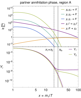
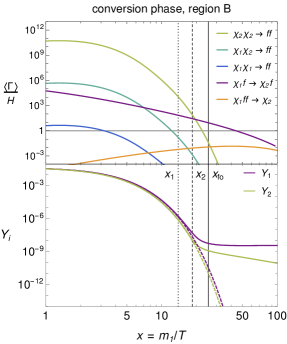
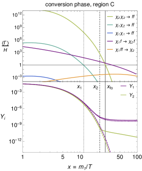
Figure 1: Evolution of the dark fermion interaction rates $\langle\Gamma\rangle$ and yields $Y$ as a function of $x=m_{1}/T$ for three i2DM benchmarks with $m_{1}=60\,$MeV, $\Delta=0.05$ and $\alpha_{D}=1/4\pi$. The relic abundance is set by partner annihilation (upper left plot), conversions in kinetic equilibrium (upper right plot) and conversions out of kinetic equilibrium (lower plot), happening in regions (A), (B) and (C), respectively. The model parameters $(\tan\theta,y)$ are set to $(0.02,4\cdot 10^{-10})$, $(0.003,10^{-9})$ and $(10^{-4},4\cdot 10^{-7})$. Top panels: interaction rates $\langle\Gamma\rangle/H\equiv\{\langle\Gamma\rangle_{ij},\langle\Gamma\rangle_{i\to j}\}\cdot n_{i}^{\rm eq}/(n_{1}^{\rm eq}H)$, $i,j=\{1,2\}$, normalized to the $\chi_{1}$ equilibrium number density and the Hubble rate. Bottom panels: comoving number densities $Y_{i}$ of dark fermions $\chi_{i}$ (solid purple and green curves) and equilibrium number densities $Y_{i}^{\rm eq}$ (dashed curves). In the lower plot, the naive $\chi_{1}$ number density obtained from integrated Boltzmann equations (dotted purple curve) is shown for comparison with the correct result from unintegrated Boltzmann equations (solid curve). See Sec. 3.2.3 for details. Vertical black lines indicate the times for $\chi_{1}$ chemical decoupling (dotted), $\chi_{2}$ chemical decoupling (dashed), and $\chi_{1}$ freeze-out (solid).

3.2 Phases of freeze-out

From the discussion in Sec. 3.1, it becomes clear that the freeze-out dynamics should be very sensitive to the parameters $y,\,\theta$ and $\Delta$. When successively decreasing the dark interaction strength $y$, we identify three different phases of freeze-out, distinguished by the processes that set the dark matter relic abundance:

1. coannihilation phase: $\Omega_{\chi}h^{2}$ set by $\chi_{1}\chi_{2}\leftrightarrow f\bar{f}$ and $\chi_{2}\chi_{2}\leftrightarrow f\bar{f}$,

2. partner annihilation phase: $\Omega_{\chi}h^{2}$ set by $\chi_{2}\chi_{2}\leftrightarrow f\bar{f}$,

3. conversion phase: $\Omega_{\chi}h^{2}$ set by $\chi_{1}f\leftrightarrow\chi_{2}f$ and/or $\chi_{2}\leftrightarrow\chi_{1}f\bar{f}$.

In addition, the thermal history of the dark matter candidate depends on whether departures from chemical or kinetic equilibrium with the bath have occurred prior to freeze-out. This critically depends on the efficiency of $\chi_{1}\leftrightarrow\chi_{2}$ conversions at the time $x_{2}$ at which $\chi_{2}$ chemically decouples. We distinguish between three regions of parameter space, where the following conditions are satisfied:

$$(\text{A}) \qquad\ \ \frac{\text{$\langle\Gamma\rangle$}_{1\to 2}}{H}(x_{2})\gtrsim 100$$ (33)

$$(\text{B}) \ 10\lesssim\frac{\text{$\langle\Gamma\rangle$}_{1\to 2}}{H}(x_{2})\lesssim 100$$ (34)

$$(\text{C}) \qquad\ \ \frac{\text{$\langle\Gamma\rangle$}_{1\to 2}}{H}(x_{2})\lesssim 10\,,$$ (35)

where $\text{$\langle\Gamma\rangle$}_{1\to 2}$ denotes the conversion rates from Eq. (32) and $H(x_{2})$ is the Hubble expansion at the time $x_{2}$. These three regions allow us to systematically study the effects of dark matter chemical and kinetic decoupling before freeze-out on the relic abundance.

Chemical decoupling of $\chi_{2}$ occurs when its (co)annihilation rate drops below the Hubble rate. If conversions $\chi_{1}\leftrightarrow\chi_{2}$ are efficient around $x_{2}$, the decoupling time can roughly be estimated using

$$r_{2}\big{(}\text{$\langle\Gamma\rangle$}_{22}(x_{2})+2\text{$\langle\Gamma\rangle$}_{21}(x_{2})\big{)}\approx H(x_{2})\,,$$ (36)

and $\chi_{2}$ decouples at the same time as $\chi_{1}$. However, if conversions are absent, $\chi_{2}$ chemically decouples around

$$\text{$\langle\Gamma\rangle$}_{22}(x_{2})\approx H(x_{2})\,.$$ (37)

Numerically we determine the time $x_{i}$ where $\chi_{i}$ chemically decouples by requiring that the density yield deviates from equilibrium by 20%,

$$x_{i}=\frac{m_{1}}{T_{i}}:\qquad\frac{Y_{i}(x_{i})}{Y_{i}^{\rm eq}(x_{i})}=1.2\,,\qquad i=\{1,2\}.$$ (38)

The classification made above allows us to understand the density evolution of the dark fermions shown in Fig. 1. The three i2DM benchmarks correspond to the freeze-out phases of partner annihilation (upper left plot) and conversion (upper right and lower plots). Partner annihilation is relevant in region (A), while conversion can prevail either in region (B) in kinetic equilibrium (upper right plot), or in region (C) beyond kinetic equilibrium (lower plot). The interplay between the different freeze-out phases and decoupling regions is shown in Fig. 2 as a function of the model parameters $y$ and $\tan\theta$ for two scenarios with fixed dark matter masses. In the upper plot of Fig. 2, the three benchmark i2DM scenarios from Fig. 1 are marked as green bullets. Below we first discuss Fig. 1 in detail and then turn to Fig. 2.

In Fig. 1, all benchmarks correspond to fixed parameters $m_{1}=60\,$MeV, $\Delta=0.05$ and $\alpha_{D}=1/4\pi$. In each of the plots, the top panel shows the evolution of the various interaction rates $\langle\Gamma\rangle$, normalized to the Hubble rate. The conversion rate $\Gamma_{1\to 2}$ that distinguishes regions (A), (B), and (C) is driven by $y\tan^{2}\theta$, see Eq. (30). It decreases when going from partner annihilation in region (A) (upper left plot) to conversion beyond kinetic equilibrium in region (C) (lower plot). The relative scaling of the interaction rates is determined by the reaction densities from Eqs. (29), (30) and (31) discussed in Sec. 2. In particular, the reaction densities for (co)annihilations, $\gamma_{ij}\sim e^{-2x}$, drop faster at low temperatures than scattering and decays, $\gamma_{i\to j}\sim e^{-x}$. The relative strength of (co)annihilations depends exponentially on the mass splitting $\Delta$ and also on the dark fermion mixing $\theta$. Due to the small splitting and mixing in the three benchmarks, partner annihilation dominates (light green), followed by coannihilation (dark green) and suppressed dark matter annihilations (blue). As mentioned in Sec. 2, conversions through scattering (purple) decrease faster with time than inverse decays (orange). Around freeze-out, however, conversions dominate over decays in all three benchmarks.

In the bottom panels of Fig. 1, we show the time evolution of the dark fermion comoving number densities, $Y_{i}(x)$, (solid) and the equilibrium yield, $Y_{i}^{\rm eq}(x)$, for comparison (dashed). In the lower plot, we also indicate the evolution that is obtained when neglecting the kinetic decoupling of dark matter (dotted). To guide the eye, we highlight the times for freeze-out and chemical decoupling with black vertical lines, determined by Eqs. (22) and (38).

We now turn our attention to Fig. 2, which illustrates the different phases of freeze-out for i2DM as a function of the dark interaction strength $y$ and the dark fermion mixing $\tan\theta$ for two fixed dark matter masses $m_{1}=60$ MeV (top) and 150 MeV (bottom). The regions (A), (B) and (C), corresponding to decreasingly efficient conversions as suggested by Eqs. (33)-(35), are delineated with dashed gray lines. The exact relations between the conversion rate and the Hubble rate along these lines are given in Eqs. (47) and (48). The observed relic abundance $\Omega_{\chi}h^{2}=0.12$ is obtained along the solid colored contours in the $(y,\tan\theta)$ plane for fixed values of the mass splitting $\Delta$. When increasing the dark matter mass $m_{1}$, the contours shift to the right, meaning that the observed abundance is obtained for larger values of $y$. This is easily understood, as all (co)annihilation and conversion rates scale as $\text{$\langle\Gamma\rangle$}_{ij},\text{$\langle\Gamma\rangle$}_{i\to j}\propto y/m_{1}^{2}$. In the upper part of the plots, all contours converge and the mass splitting $\Delta$ plays no role in setting the relic abundance. Here the abundance is set by pair annihilations $\chi_{1}\chi_{1}\to f\bar{f}$, see Eq. (29). In Sec. 5, we will see that laboratory searches exclude this region of parameter space. As a result, we focus on dark matter candidates with small couplings, corresponding to the phases of coannihilation and partner annihilation in region (A), and on conversions in regions (B) and (C).

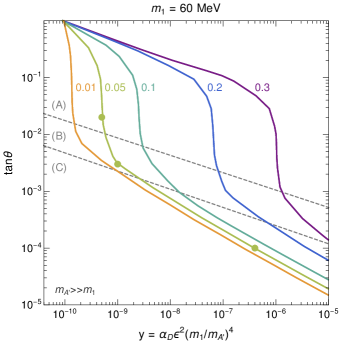
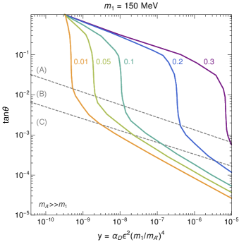
Figure 2: Dark matter relic abundance for i2DM as a function of the dark interaction strength, $y$, and the dark fermion mixing, $\tan\theta$. The dark matter mass is fixed to $m_{1}=60\,$MeV (top) and 150 MeV (bottom). The observed abundance $\Omega_{\chi}h^{2}=0.12$ is obtained along the colored contours for different dark fermion mass splittings $\Delta=0.01\dots 0.3$. The decoupling regions (A), (B) and (C) are separated by dashed gray lines, which satisfy Eqs. (47) and (48). In region (A), the dark sector is in chemical and kinetic equilibrium with the bath. In regions (B) and (C), $\chi_{1}$ successively decouples from chemical and kinetic equilibrium with $\chi_{2}$ prior to freeze-out. In the top panel, the bullets on the green contour for $\Delta=0.05$ mark the position of the three i2DM benchmarks displayed in Fig. 1.

In region (A), efficient conversion rates satisfying Eq. (33) keep $\chi_{1}$ in chemical and kinetic equilibrium with the thermal bath until freeze-out. In particular, efficient conversions ensure that $\chi_{1}$ and $\chi_{2}$ have equal chemical potentials, so that their number densities are related by

$$\frac{n_{1}}{n_{2}}=\frac{n_{1}^{\rm eq}}{n_{2}^{\rm eq}}\,.$$ (39)

In this case, the freeze-out conditions are similar to the ones of a thermal WIMP and the observed relic dark matter abundance is obtained for a freeze-out time Griest:1990kh ; Gondolo:1990dk ; Edsjo:1997bg

$$x_{\rm WIMP}\simeq 25\,.$$ (40)

This is illustrated by the density evolution for the benchmark in the upper left plot of Fig. 1, which corresponds to the upper green bullet in the upper plot of Fig. 2. At large $\tan\theta$ of region (A), we note the rapid bending of the curves. This happens when coannihilations and pair annihilations of the lightest dark state start playing significant role at decoupling of $\chi_{1}$. The relative impact of the mentioned reactions is not important for our discussion as long as condition (A) is satisfied.

When entering in region (B), defined by Eq. (34), conversion processes are less efficient and the rates $\text{$\langle\Gamma\rangle$}_{1\to 2}(x_{2})$ are about ten to one hundred times larger than the Hubble rate. As a result, the dark matter density departs from chemical equilibrium prior to freeze-out. The effect is visible in the second benchmark displayed in the upper right plot of Fig. 1, corresponding to the second green bullet in the upper plot of Fig. 2.

Once the conversion rate $\text{$\langle\Gamma\rangle$}_{1\to 2}(x_{2})$ is further suppressed, dark matter cannot be expected to be kept in kinetic equilibrium until freeze-out. We enter region (C), defined by Eq. (35) and illustrated by a benchmark in the lower plot of Fig. 1, corresponding to the lower green bullet of the upper plot of Fig. 2. To quantify the effect of kinetic decoupling, in Fig. 1 we display the physical dark matter yield obtained by respecting kinetic decoupling (solid purple curve) compared to the same yield obtained when neglecting kinetic decoupling (dotted purple curve).

In what follows, we will discuss the physics of the three freeze-out phases in detail, paying particular attention to non-equilibrium effects in the conversion phase. Further details about the computation of the dark matter relic abundance in the presence of chemical and kinetic decoupling can also be found in App. B.

3.2.1 Coannihilation

Coannihilation sets the relic abundance when the rate of $\chi_{1}\chi_{2}\leftrightarrow f\bar{f}$ is larger than the Hubble rate and dominates over dark matter pair annihilations $\chi_{1}\chi_{1}\leftrightarrow f\bar{f}$ around the freeze-out time, i.e., when

$$\text{$\langle\Gamma\rangle$}_{12}(x_{\rm fo})>\text{$\langle\Gamma\rangle$}_{11}(x_{\rm fo})\,.$$ (41)

According to Eqs. (25) and (29), in i2DM the ratio of these rates scales as

$$\frac{\text{$\langle\Gamma\rangle$}_{11}(x)}{\text{$\langle\Gamma\rangle$}_{12}(x)}\sim\frac{n_{1}^{\rm eq}}{n_{2}^{\rm eq}}\,\tan^{2}\theta\sim e^{x\Delta}\tan^{2}\theta\,.$$ (42)

One might deduce that coannihilation sets the relic abundance if $e^{x_{\rm fo}\Delta}\tan^{2}\theta\lesssim 1$. However, this is only a necessary condition, because in this regime the relic abundance could also be driven by partner annihilation $\chi_{2}\chi_{2}\to f\bar{f}$. To determine the relative impact of partner annihilation, one needs to consider the weighted ratio of coannihilation and partner annihilation rates, $r_{1}\text{$\langle\Gamma\rangle$}_{12}(x)/r_{2}\text{$\langle\Gamma\rangle$}_{22}(x)$. In i2DM, this ratio scales as $e^{x\Delta}\tan^{2}\theta$, exactly as in Eq. (42). As a result, in the coannihilation phase the comoving number density $Y_{1}(x)$ freezes once the weighted sum of coannihilation and partner annihilation drops below the Hubble rate,

$$2r_{1}\text{$\langle\Gamma\rangle$}_{12}(x_{\rm fo})+r_{2}\text{$\langle\Gamma\rangle$}_{22}(x_{\rm fo})\approx H(x_{\rm fo})\,,\qquad x_{\rm fo}\simeq x_{\rm WIMP}\,.$$ (43)

The relic dark matter abundance is set around the freeze-out temperature of a thermal WIMP. Freeze-out through coannihilation is realized in the upper part of region (A) in Fig. 2. Due to the scaling $\text{$\langle\Gamma\rangle$}_{12}\sim y\,\sin^{2}(2\theta)$, the relic abundance contours tend to larger interaction strength $y$ at smaller mixing $\theta$ in this regime.

In the coannihilation phase, i2DM resembles iDM, where the $\xi_{1}-\xi_{2}$ couplings of Eq. (15) prevail and coannihilations $\xi_{1}\xi_{2}\to f\bar{f}$ are the dominant number-changing interactions of the dark matter candidate $\xi_{1}$ with the bath. However, lowering the dark interaction strength $y$ leads to inefficient coannihilation around freeze-out. In iDM, this results in an overabundance of dark matter. In i2DM, suppressed coannihilations can be compensated by efficient partner annihilations and conversions, thus explaining the observed dark matter abundance even if the dark sector is feebly coupled.

3.2.2 Partner annihilation

If the coannihilation rate is suppressed compared to the Hubble rate around $x=x_{\rm WIMP}$, the relic DM abundance can be set by partner annihilations $\chi_{2}\chi_{2}\to f\bar{f}$. In this phase, the freeze-out condition reads

$$r_{2}\,\text{$\langle\Gamma\rangle$}_{22}(x_{\rm fo})\approx H(x_{\rm fo})\,,\qquad x_{\rm fo}\simeq x_{\rm WIMP}\,.$$ (44)

As in the coannihilation phase, the freeze-out time is fixed to $x_{\rm fo}\simeq x_{\rm WIMP}$, up to a moderate logarithmic dependence on the model parameters Griest:1990kh . In Fig. 2, the phase of partner annihilation lies in region (A) and is characterized by vertical lines. Due to the scaling $r_{2}\langle\Gamma_{22}\rangle\sim y\cos^{4}\theta\,e^{-2x\Delta}$, the relic dark matter abundance is essentially independent of the mixing as $\cos^{4}\theta\approx 1$. To obtain the observed abundance, variations of the dark interaction strength $y$ can be compensated by the mass splitting $\Delta$, as illustrated by the various contours. In the partner annihilation phase, $\chi_{1}\leftrightarrow\chi_{2}$ conversions have to be efficient enough to satisfy the decoupling condition from Eq. (33). As a consequence, $\chi_{1}$ and $\chi_{2}$ chemically decouple from the bath around the same time. This is visible in the upper left plot of Fig. 1. Notice that $\chi_{2}\to\chi_{1}$ decays happen on a time scale shorter than the period of chemical decoupling and do not affect the freeze-out time $x_{\rm fo}\approx x_{\rm WIMP}$.

Whenever coannihilation or partner annihilation set the relic abundance, dark matter is in chemical and kinetic equilibrium until decoupling. In this case, the evolution equations from Eq. (23) can be reduced to one single integrated Boltzmann equation, written in terms of the total number density of all dark particles, $n=\sum_{i}n_{i}$, as commonly used for thermal WIMPs Griest:1990kh ; Edsjo:1997bg . The dark matter abundance can be computed with any of the available Boltzmann solvers Belanger:2018ccd ; Bringmann:2018lay ; Ambrogi:2018jqj , which explicitly make use of Eq. (39). For the computations in this work we have used our own Boltzmann solver. We have verified that our results for the relic abundance in region (A) in Fig. 2 and in the left panel of Fig. 1 agree with the results obtained from micrOMEGAs Belanger:2018ccd .

3.2.3 Conversion

As we discussed above, partner annihilation can set the relic dark matter abundance even if $\chi_{1}\chi_{1}\to f\bar{f}$ and $\chi_{1}\chi_{2}\to f\bar{f}$ annihilations are suppressed. If the dark fermion mixing $\theta$ is very small, $\chi_{1}\leftrightarrow\chi_{2}$ conversion rates can be comparable to or even fall below the Hubble rate around $\chi_{2}$ chemical decoupling, as in Eqs. (34) and (35). The dark matter abundance is now set by conversion processes, i.e., by coscattering and/or (inverse) decays.

In i2DM, conversion-driven freeze-out can occur in regions (B) and (C) in Fig. 2, Here coscattering dominates over decays in the thermal history around freeze-out. Due to the scaling $\text{$\langle\Gamma\rangle$}_{1\to 2}\propto\sin^{2}(2\theta)$, the contours of constant $\Omega_{\chi}h^{2}$ are sensitive to the mixing angle $\theta$. For a fixed interaction strength $y$ and mass splitting $\Delta$, the relic abundance in this regime is generally larger than what one would expected from partner annihilation. The reason is that $\chi_{1}\leftrightarrow\chi_{2}$ conversions are less efficient and the dark matter yield $Y_{1}(x)$ can start to deviate from the equilibrium yield $Y_{1}^{\rm eq}(x)$ well before the freeze-out time $x=x_{\rm fo}$  Garny:2017rxs ; DAgnolo:2018wcn . The latter effect is illustrated in the upper right and lower plots of Fig. 1. The increased yield has to be compensated by a larger interaction strength $y$, causing the contours in Fig. 2 to bend towards the lower right corner. Notice that efficient partner annihilation is essential for conversions to explain the observed relic abundance. Suppressed partner annihilations would result in an overabundance of dark matter.

To describe deviations of the dark matter density from chemical and kinetic equilibrium within the conversion phase, it is convenient to distinguish three key moments:

1. the time $x_{1}$ at which $\chi_{1}$ chemically decouples from the bath;

2. the time $x_{2}$ at which $\chi_{2}$ chemically decouples from the bath;

3. the dark matter freeze-out time $x_{\rm fo}$, which can differ from $x_{\rm WIMP}\simeq 25$ in the conversion phase.

Numerically, we determine $x_{1}$, $x_{2}$ and $x_{\rm fo}$ using Eqs. (38) and (22). Deviations of the dark matter density from chemical equilibrium around freeze-out typically occur for

$$x_{1}\lesssim x_{2}<x_{\rm fo}\,.$$ (45)

Deviations from chemical and kinetic equilibrium can occur for

$$x_{1}\ll x_{2}<x_{\rm fo}\,.$$ (46)

Thanks to efficient elastic scattering, the dark partner $\chi_{2}$ is kept in kinetic equilibrium with the bath throughout the dark matter freeze-out process and in particular for $x>x_{2}$ after $\chi_{2}$ chemical decoupling.

Deviations from chemical equilibrium

If $x_{1}\lesssim x_{2}$, conversions are barely efficient during $\chi_{2}$ chemical decoupling, as in Eq. (34). This scenario corresponds to region (B) in Fig. 2. Numerically we find that the boundary between regions (A) and (B) corresponds to

$$\text{$\langle\Gamma\rangle$}_{1\to 2}(x_{2})=200\,H(x_{2})\,,$$ (47)

using Eq. (38) to evaluate $x_{2}$. Below this boundary, the $\chi_{1}$ density departs from chemical equilibrium before $\chi_{2}$. This effect is illustrated for a benchmark in the upper right plot of Fig. 1, where the freeze-out process for $Y_{1}(x)$ terminates around $x_{\rm fo}>x_{1}$. At that time, we expect that conversions are still sufficiently active to keep $\chi_{1}$ in kinetic equilibrium with the thermal bath via $\chi_{2}$. In particular, we assume that the dark matter distribution function $f_{1}(x,q)$ is well approximated by the Boltzmann distribution $f_{1}^{\rm eq}(x,q)$ throughout the entire evolution process.

To account for deviations from chemical equilibrium in region (B), the Boltzmann equations commonly used for (co)annihilating dark matter Griest:1990kh have to be supplemented by explicitly including the conversion rate in the coupled system of evolution equations for $Y_{1}(x)$ and $Y_{2}(x)$. For details on our implementation of the Boltzmann equations we refer the reader to App. B.1.

Deviations from chemical and kinetic equilibrium

For $x_{1}\ll x_{2}$, conversions become inefficient before $\chi_{2}$ chemically decouples, and the condition of Eq. (35) is satisfied. This scenario corresponds to region (C) in Fig. 2. Numerically, we find that the boundary between regions (B) and (C) is given by

$$\text{$\langle\Gamma\rangle$}_{1\to 2}(x_{2})=20\,H(x_{2})\,,$$ (48)

with $x_{2}$ evaluated with Eq. (38). Below this line, the mixing $\theta$ is so small that conversions fail to keep dark matter in kinetic equilibrium. This effect is visualized in the lower panel of Fig. 1: The dark matter yield $Y_{1}(x_{\rm fo})$ including departures from kinetic equilibrium (solid curve) is larger than under the assumption of kinetic equilibrium (dotted curve). The time between dark matter chemical decoupling and freeze-out is now stretched over a larger range between $x_{1}$ and $x_{\rm fo}$.

In region (C), the phase-space density $f_{1}(x,q)$ is expected to deviate significantly from a Maxwell-Boltzmann distribution for $x>x_{1}$. To account for deviations from kinetic equilibrium, the unintegrated Boltzmann equations from Eq. (23) have to be solved for the momentum-dependent phase-space density of $\chi_{1}$ DAgnolo:2017dbv ; Garny:2017rxs . Further details are given in App. B.2. Using our own implementation, we obtain the solid purple curve in the lower plot of Fig. 1. For comparison, we show the evolution of $Y_{1}(x)$ obtained using the integrated Boltzmann equations relevant in region (B), but neglecting deviations from kinetic equilibrium (dotted line). The deviations are modest, ranging around 35%.

Throughout this work and in particular in Figs. 2, 3 and 4, we use the set of integrated Boltzmann equations from App. B.1, unless specified otherwise. This method is computationally much faster than solving the unintegrated Boltzmann equations and reproduces the exact results to a good approximation.

4 Bounds from cosmology and astrophysics

The parameter space of i2DM is constrained by several observables in cosmology and astrophysics. In general, the presence of light new particles with masses in the MeV-GeV range affects the thermal history of the universe. Two main effects can be distinguished. First, the presence of additional particles in the thermal bath changes the evolution of the Hubble expansion and of the entropy density of the universe. This may significantly affect the QCD phase transition, Big Bang Nucleosynthesis (BBN), the Cosmic Microwave Background (CMB) or supernova cooling. Second, the annihilation or decay of new particles injects energy into the thermal plasma by inducing excitations, ionisation and heating. Such effects can modify BBN and the CMB compared to the predictions of the cosmological standard model.

In this section, we study the impact of i2DM dark fermions on cosmological and astrophysical observables. In Sec. 4.1, we consider bounds on particles that freeze-out around the QCD phase transition, at temperatures $T_{\rm QCD}\sim 200\,$MeV. In Sec. 4.2, we derive constraints from BBN around $T_{\rm BBN}\sim 0.1\,$MeV. In Sec. 4.3, we discuss effects on the CMB around $T\sim 1\,$eV, while in Sec. 4.4 we report on the constraints from the measurement of the effective number of neutrinos, $N_{\rm eff}$, at the CMB and BBN times. Finally, in Sec. 4.5, we consider constraints on dark sector particles escaping supernovae.

4.1 QCD phase transition

If new particles freeze-out around the GeV scale, the QCD phase transition around $T_{\rm QCD}\sim 200\,$MeV affects the relic abundance Steigman:2012nb . The confinement of quarks and gluons into hadrons reduces the effective number of relativistic degrees of freedom contributing to the entropy density, $h_{\rm eff}$ Olive:1980dy . Calculations of $h_{\rm eff}$ around the phase transition are subject to significant uncertainties, leading to variations of about ten percent in the relic abundance Hindmarsh:2005ix ; Laine:2006cp ; Drees:2015exa . However, the effect of the QCD phase transition on the thermal evolution of light new particles can be much larger than the mentioned uncertainties. In particular, it can affect the relic abundance of dark matter candidates that freeze out during or shortly after the phase transition.

In Sec. 3.2, we have investigated the freeze-out dynamics of i2DM separately from effects of the QCD phase transition. If the freeze-out occurs in thermal equilibrium, dark matter candidates with masses

$$m_{1}\lesssim 1\,\text{GeV}$$ (49)

decouple from the bath around $T_{\rm WIMP}\approx m_{1}/x_{\rm WIMP}\ll T_{\rm QCD}$, late enough to neglect effects of the QCD phase transition on dark matter decoupling Drees:2015exa . In i2DM this holds in the phases of coannihilation and partner annihilation. However, in the conversion phase, Eq. (49) is not necessarily satisfied because chemical and kinetic equilibrium are not guaranteed until freeze-out, see Sec. 3.2.3. In this case, the dark fermions decouple from chemical equilibrium at earlier times $x_{1,2}\lesssim x_{\rm WIMP}$, which might be affected by the QCD phase transition if the corresponding decoupling temperature is similar to $T_{\rm QCD}$. On the other hand, dark matter freeze-out is expected to be unaffected by the phase transition, because the dark states decouple at temperatures $T\lesssim T_{\rm WIMP}$. In any case, bounds from laboratory searches exclude i2DM dark matter candidates with masses near 1 GeV, see Sec. 5. Even if non-equilibrium effects can change the decoupling times of the dark states, we do not expect effects from the QCD phase transition to affect the thermal history of dark matter candidates with masses well below the GeV scale.

4.2 Big Bang Nucleosynthesis

The formation of primordial light nuclei starts around $T_{\rm BBN}\sim 0.1\,$MeV. New physics can affect the nuclei abundances in multiple ways. First of all, new dark particles can affect BBN by modifying the Hubble rate or the entropy density of the universe. Second, efficient annihilation of MeV-GeV-scale dark particles to electrons or photons may alter the rate at which light elements form Depta:2019lbe . Third, dark particles decaying to electrons or photons at later times can destroy the already formed primordial nuclei Depta:2020zbh ; Depta:2020mhj . In i2DM, dark matter annihilation and dark partner decays around $T\sim T_{\rm BBN}$ are not strong enough to cause observable effects. Late decays of dark partners with lifetimes $\tau_{2}>t_{\rm BBN}$, however, can destroy the newly formed elements through photodisintegration and constrain parts of the i2DM parameter space. Below we will discuss photodisintegration in i2DM in detail and briefly argue why annihilation and decays during BBN are not efficient.

For annihilating dark matter during BBN, a lower mass bound of $m_{\rm DM}\gtrsim 10\,$MeV has been derived in Depta:2019lbe . This bound applies for vanilla WIMP annihilation with $\langle\sigma v\rangle\approx 10^{-26}-10^{-28}$ cm³/s. In the coannihilation and conversion phases of i2DM, however, the cross section for annihilations $\chi_{1}\chi_{1}\to\{e^{+}e^{-},\gamma\gamma\}$ is much smaller than for vanilla WIMPs, resulting in weaker bounds on the dark matter mass. We expect these bounds to be superseded by constraints on $\Delta N_{\rm eff}$ from CMB measurements, see Sec. 4.4.

On the other hand, decays $\chi_{2}\to\chi_{1}\ell^{+}\ell^{-}$ and $\chi_{2}\to\chi_{1}\gamma\gamma$ of dark partners with MeV-GeV masses and lifetimes $\tau_{2}>10^{3}\,$s can produce an electromagnetic cascade of photons with energies above the binding energy of light nuclei, consequently disintegrating them. Disintegration is efficient only if the emitted photons do not lose their energy too rapidly before reaching the target nucleus. This condition is satisfied if the energy of the photons lies below the di-electron threshold, $E^{\rm th}_{e^{+}e^{-}}\simeq m_{e}^{2}/(22\,T)$ Hufnagel:2018bjp . On the other hand, for photodisintegration to take place, $E^{\rm th}_{e^{+}e^{-}}$ should lie well above the binding energy of light elements, corresponding to temperatures below a few keV. Photodisintegration is thus efficient for photon energies

$$\mathcal{O}(\text{keV})\lesssim E_{\gamma}\lesssim\frac{m_{e}^{2}}{22\,T}\,.$$ (50)

We calculate the effects of photodisintegration on the nuclei abundances starting from a continuous electron spectrum originating from $\chi_{2}\to\chi_{1}e^{+}e^{-}$ decays. We neglect loop-suppressed direct photon production, $\chi_{2}\to\chi_{1}\gamma\gamma$, as well as final-state radiation, resulting in a conservative bound on the electromagnetic flux obtained from partner decays Forestell:2018txr . To investigate photodisintegration for i2DM, we use the public code ACROPOLIS Depta:2020mhj . The code calculates the modified primordial abundances of light elements induced by photodisintegration, accounting for the redistribution of the energy injected by the decaying dark particle in the plasma. In particular, ACROPOLIS includes the exponential suppression in the photon spectrum for energies $E_{\gamma}>E^{th}_{e^{+}e^{-}}$, which was neglected in previous studies, up to energies $E_{\gamma}<E_{0}$, where $E_{0}$ is a model-dependent upper limit on the photon spectrum. We set $E_{0}$ to the maximum kinematically allowed energy. For the initial abundances of light nuclei, we use the Standard BBN prediction extracted from the code AlterBBN ARBEY20121822 . The input number density of $\chi_{2}$ is extracted from our system of Boltzmann equations.

The resulting constraints from photodisintegration on partner decays in i2DM are shown in Fig. 3. Bounds on the displayed parameter space are only visible in the lower right corner of the left panel with $\tan\theta=10^{-4},\,\Delta=0.05$, far from the correct relic abundance (the green dotted line). At larger $\tan\theta$, photodisintegration is not efficient because the dark partners decay too early. The lifetime of $\chi_{2}$ also determines the upper edge of the excluded region. At dark matter masses, $m_{1}\lesssim 120\,$MeV, photodisintegration becomes inefficient due to the small absolute mass splitting between the dark fermions, $m_{2}-m_{1}$, which causes too soft decay products. For larger mass splittings $\Delta=0.1$, in the right panel, photodisintegration is sensitive to smaller dark matter masses. However, the lifetime of $\chi_{2}$ is generally smaller so that smaller couplings would be necessary for photodesintegration to take place. As a consequence, the excluded region lies below the plotted area in Fig. 3 and BBN bounds are irrelevant for viable i2DM relics. In summary, in i2DM photodisintegration excludes dark partners with lifetimes much larger than in cosmologically viable scenarios.

4.3 Cosmic Microwave Background

Dark sector particles that annihilate or decay around the time of recombination can affect the overall shape of the CMB black body spectrum, as well as its temperature and the polarization anisotropy spectra. Measurements of the CMB temperature and the polarization anisotropy spectra set strong constraints on the annihilation cross section of WIMP-like dark matter and also on decaying new particles with lifetimes $\tau>10^{13}\,$s. For particles with shorter lifetimes, extra constraints can be obtained by studying deformations of the blackbody spectrum before recombination, usually referred to as spectral distortions. In addition, dark matter with couplings to neutrinos, photons or electrons can shift the effective number of neutrinos around the time of recombination $\Delta N_{\rm eff}(T_{\rm CMB})$, and affect the CMB anisotropies. We will discuss the constraints arising from $\Delta N_{\rm eff}$ in Sec. 4.4.

Charged SM particles that can arise from decays or annihilations of dark particles can inject energy into the plasma in the form of heat. Heat injections at redshifts $z\lesssim 2\cdot 10^{6}$ induce spectral distortions in the CMB. Measurements of spectral distortions are sensitive to dark particles with lifetimes $\tau\gtrsim 10^{4}\,$s. However, existing bounds from the COBE-FIRAS experiment Fixsen:1996nj are largely superseded by the BBN bounds discussed in Sec. 4.2. Future CMB missions similar to PiXie could strengthen the bounds on particles with lifetimes $\tau\gtrsim 10^{4}\,$s by up to two orders magnitude Poulin:2015opa ; Lucca:2019rxf . In contrast, BBN bounds are not expected to improve as much in the future.

Charged particles from decays or annihilations of dark sector particles can also ionize the plasma. Ionization at redshifts $z\lesssim 10^{3}$ modifies the CMB anisotropy spectra. This ionized fraction of the energy deposit induces a broadening of the surface of last scattering; for instance, it attenuates the CMB power spectrum on scales smaller than the width of the surface Padmanabhan:2005es . Measurements by the Planck collaboration constrain this effect and set strong upper limits on the cross section for $s$-wave dark matter annihilation Planck:2018vyg . In i2DM, dark matter annihilation $\chi_{1}\chi_{1}\to f\bar{f}$ is suppressed well below these limits.

Compared to ionization effects on the CMB anisotropies, searches for dark matter annihilation in indirect detection experiments impose much weaker bounds in the MeV-GeV mass range Leane:2018kjk ; e-ASTROGAM:2017pxr . Future missions such as e-astrogram e-ASTROGAM:2017pxr can provide competitive bounds on the annihilation cross section, which however are still far above the suppressed annihilation rates in i2DM.

4.4 Effective number of neutrinos $N_{\rm eff}$

As mentioned above, stable dark matter coupled to neutrinos, photons or electrons can change the effective number of neutrinos by $\Delta N_{\rm eff}$. This modification can affect the abundance of light nuclei (set at $T_{\rm BBN}\sim 0.1$ MeV) and the CMB anisotropies (set around $T_{\rm CMB}\sim 0.4$ eV). Both measurements can thus set bounds on $\Delta N_{\rm eff}$.

Efficient dark matter scattering with the electromagnetic or neutrino bath can induce an entropy transfer to these species after neutrino decoupling (at $T_{\nu}\sim$ MeV), thus modifying the neutrino-to-photon temperature ratio compared to the SM prediction. In practice, this information is encapsulated in $\Delta N_{\rm eff}$. For dark matter that only couples to neutrinos, the entropy transfer reheats the neutrino bath and induces a positive shift $\Delta N_{\rm eff}>0$. For dark matter coupling to either electrons or photons, the electromagnetic bath gets reheated, which induces a negative shift $\Delta N_{\rm eff}<0$.

To estimate the effect of light dark particles on $N_{\rm eff}$, we follow the detailed analysis of Escudero:2018mvt , which uses the constraint on $\Delta N_{\rm eff}$ by the Planck collaboration Planck:2018vyg ,

$$N_{\rm eff}(T_{\rm CMB})=2.99^{+0.34}_{-0.33}\qquad\text{at }95\%\,\text{CL}.$$ (51)

From this constraint, the authors of Escudero:2018mvt derive a lower bound on the mass of a Dirac fermion dark matter candidate that couples efficiently to electrons, finding

$$m_{\rm DM}>9.2\,{\rm MeV}\qquad\text{at }95\%\,\text{CL}.$$ (52)

This result agrees with the estimates in Boehm:2013jpa ; Depta:2019lbe , for instance. We emphasize that a modification of $N_{\rm eff}$ can only be observed in CMB data if Boehm:2013jpa

• the dark matter is in kinetic equilibrium with either electrons, photons or neutrinos at temperatures above and below $T_{\nu}\sim$ MeV;

• the dark matter becomes non-relativistic at temperatures $T\lesssim T_{\nu}$, typically for masses below a few tens of MeV.

As a result, in i2DM the bound from Eq. (52) only holds in regions (A) and (B), defined in Eqs. (33) and (34), where the dark fermions are in kinetic equilibrium prior to freeze-out. For simplicity, we restrict ourselves to dark matter candidates with $m_{1}>10\,$MeV in all three regions.

4.5 Supernova cooling

Feebly interacting dark-sector particles can be produced in proto-neutron stars and freely escape them. The energy carried by the dark particles speeds up the supernova cooling and therefore can constrain models with light dark sectors. In i2DM, dark fermions are mostly produced through decays of dark photons produced in bremsstrahlung during neutron-proton collisions or directly in collisions of light SM fermions Chang:2018rso . Existing bounds on the cooling of the supernova SN1987A Kamiokande-II:1987idp ; PhysRevLett.58.1494 constrain the i2DM parameter space only at very small couplings that are irrelevant for our purposes. Based on the results for iDM in Chang:2018rso , we estimate that in i2DM supernova cooling constrains dark couplings up to at most $y\approx 10^{-13}$ for masses $m_{1}\lesssim 200\,$MeV; a parameter space where the dark matter relics would be overabundant. The bounds could potentially be even weaker if different core-collapse simulations were used Bar:2019ifz . Valid i2DM relics are thus not subject to bounds from supernova cooling.

5 Laboratory searches

In this section we discuss the phenomenology of inelastic dark matter in direct detection experiments, at particle colliders and at fixed-target experiments. Despite the original motivation of inelastic dark matter to evade direct detection, recent investigations reveal sensitivity to certain scenarios of iDM. Colliders and fixed-target experiments set strong bounds on the parameter space of iDM. We show that i2DM can evade some of these bounds, but can be conclusively tested at future experiments. Indirect detection searches are not sensitive to i2DM, because the pair-annihilation rate of dark matter is suppressed by small kinetic mixing and small dark fermion mixing, well below the reach of current and projected future experiments.

5.1 Direct detection

In scenarios of feebly interacting inelastic dark matter, elastic scattering $\chi_{1}X\to\chi_{1}X$ off nucleons or electrons, $X=n$ or $e$, is suppressed below the sensitivity of current direct detection experiments. In the MeV-GeV mass range, the recoil energy in nucleon scattering is typically too small to be observed, but electron recoils are a promising road to detection Ema:2018bih . The strongest current bound on dark matter-electron scattering by Xenon 1T lies around $\sigma(\chi_{1}e\to\chi_{1}e)\sim 10^{-40}$ cm² XENON:2019gfn for $m_{1}\approx 100\,$MeV. For comparison, in i2DM with $m_{1}=100\,$MeV, $m_{A^{\prime}}=3m_{1}$ and large mixings $\sin\theta=0.1$ and $\epsilon=0.02$, the predicted cross section is $\sigma(\chi_{1}e\to\chi_{1}e)=6\times 10^{-41}\,{\rm cm}^{2}$. Future direct detection experiments might reach a higher sensitivity to dark matter-electron scattering. Whether they can reach i2DM sensitivity will depend on the progress in collider searches (see Sec. 5.3), which can probe kinetic mixing down to $\epsilon\approx 10^{-3}$ and potentially suppress the target cross section as $\sigma\sim\epsilon^{2}$.

If the mass splitting $\Delta$ between the dark states is smaller than a few 100 keV, inelastic up-scattering $\chi_{1}n\to\chi_{2}n$ can produce an observable nuclear recoil signal, provided that the threshold of the experiment is low enough to detect the recoil energy Tucker-Smith:2001myb ; Bramante:2016rdh .

For larger mass splitting, up-scattering can be observable if dark matter is accelerated through interactions with cosmic rays in the atmosphere around the earth Bringmann:2018cvk : The dark matter candidate $\chi_{1}$ scatters inelastically off cosmic rays, mostly protons, via $\chi_{1}p\to\chi_{2}p$. Subsequent decays $\chi_{2}\to\chi_{1}f\bar{f}$ produce a relativistic component of dark matter, which passes the energy threshold for $\chi_{1}n\to\chi_{2}n$ scattering in experiments Bell:2021xff .

Dark partners produced from cosmic-ray reactions can induce nuclear recoils via down-scattering $\chi_{2}n\to\chi_{1}n$, provided that their lifetime is long enough to reach the experiment Graham:2010ca ; Bell:2021xff ; CarrilloGonzalez:2021lxm . Down-scattering off electrons $\chi_{2}e\to\chi_{1}e$ is an interesting alternative, which can also address the current excess of electron recoils at Xenon1T Aboubrahim:2020iwb . For inelastic dark matter, efficient down-scattering only occurs if the lifetime is longer than several years Bell:2021xff , corresponding to mass splittings much smaller than those considered in this work.

For i2DM, we expect that the rates for up-scattering and down-scattering are generally suppressed compared to iDM, due to the smaller $A^{\prime}\chi_{1}\chi_{2}$ coupling proportional to $\tan\theta$. On the other hand, in i2DM scenarios with small mass splitting, dark partners produced from cosmic-ray up-scattering are long-lived enough so that a substantial fraction of them could reach the detector before decaying. In this case, elastic scattering via $\chi_{2}n\to\chi_{2}n$ should dominate and leave an interesting characteristic signature of i2DM. In such scenarios, also down-scattering is expected. If the dark states are heavy and compressed enough to induce an observable nuclear recoil, up-scattering of i2DM off cosmic rays followed by elastic scattering off nuclei in the detector could be directly probed at experiments with a low energy threshold, cf. Ref. CarrilloGonzalez:2021lxm . A dedicated analysis of i2DM at direct detection experiments goes beyond the scope of this work, but is a promising direction for future research.

5.2 Electroweak precision observables

A general bound on kinetic mixing of a dark photon is obtained from electroweak precision tests. In electroweak observables measured at LEP, Tevatron and the LHC, kinetic mixing modifies the $Z$ boson’s mass and couplings to SM fermions at $\mathcal{O}(\epsilon^{2})$. For dark photons with masses well below the $Z$ resonance, a global fit to electroweak precision data yields a 95% CL upper bound of Curtin:2014cca

$$\epsilon\lesssim 0.02\qquad\text{for}\qquad m_{A^{\prime}}\lesssim 10\,\text{GeV};$$ (53)

stronger bounds apply for dark photons with masses closer to the $Z$ pole. For $m_{A^{\prime}}\lesssim 10\,$GeV, slightly stronger bounds have also been obtained from $e^{\pm}$ scattering off protons at HERA Kribs:2020vyk .

5.3 Collider searches

At $e^{+}e^{-}$ colliders, dark fermions coupling via a dark photon can be produced via three main processes:

$$e^{+}e^{-} \to A_{D}\gamma\to\chi_{1}\chi_{1}\gamma$$ (54)

$$e^{+}e^{-} \to A_{D}\gamma\to\chi_{1}\chi_{2}\gamma\to\chi_{1}\chi_{1}\ell^{+}\ell^{-}\gamma\qquad\qquad\text{ (iDM)}$$

$$e^{+}e^{-} \to A_{D}\gamma\to\chi_{2}\chi_{2}\gamma\to\chi_{1}\ell^{+}\ell^{-}\chi_{1}\ell^{+}\ell^{-}\gamma\qquad\text{(i2DM)}.$$

In models of inelastic dark matter, the first process is suppressed by construction. The second process dominates in iDM scenarios, which typically rely on the coupling of the dark photon to $\chi_{1}$ and $\chi_{2}$. The third process is characteristic of i2DM, since the coupling $A_{D}\chi_{1}\chi_{2}$ is suppressed by $\tan\theta$ and the dark photon mostly decays via $A_{D}\to\chi_{2}\chi_{2}$, see Eq. (9). Dark photon decays into SM fermions are suppressed as $\epsilon^{2}\alpha/\alpha_{D}$, so that resonance searches at BaBar BaBar:2014zli and LHCb LHCb:2017trq ; LHCb:2020ysn are not sensitive to the scenarios investigated in this work.

Collider signals of inelastic dark matter depend on whether the dark partners decay within or outside the detector. Below the hadronic threshold, the lifetime of $\chi_{2}$ is mostly determined by $\chi_{2}\to\chi_{1}\ell^{+}\ell^{-}$ decays, which strongly depend on $\epsilon\tan\theta$ and the mass splitting $\Delta$, see Eq. (14). If one or two dark partners decay within the detector, the signature consists of one or two prompt or displaced vertices of charged leptons, in association with a photon and missing energy. In iDM, the phenomenology of this signature has been investigated in detail for the Belle II experiment Duerr:2019dmv ; Mohlabeng:2019vrz ; Kang:2021oes . For sufficiently large mass splitting $\Delta$, Belle II will be able to probe scenarios of iDM in the GeV range.

For a smaller mass splitting, the decay products of $\chi_{2}$ are too soft to be detected, leading to a signal with a photon and missing energy. The same signature is expected if $\chi_{2}$ decays outside the detector. A search for mono-photon signals at BaBar has set an upper bound on the kinetic mixing of invisible dark photons BaBar:2017tiz ,

$$\epsilon\lesssim 10^{-3}\qquad\text{for}\qquad m_{A^{\prime}}\lesssim 5\,\text{GeV}.$$ (55)

In iDM, this bound excludes most of the parameter space for dark matter candidates below the GeV scale. A similar search at Belle II can probe even smaller dark sector couplings and thereby improve the sensitivity to iDM Duerr:2019dmv .

In i2DM, the dark photon decays close to its production point due to efficient $A^{\prime}\to\chi_{2}\chi_{2}$ decays. However, the dark partners have larger decay lengths than in iDM, because $\chi_{2}\to\chi_{1}f\bar{f}$ decays are suppressed by $\tan^{2}\theta$, see Eq. (14). Therefore the dark photon does not leave any trace in the detector and the bound of Eq. (55) from BaBar’s mono-photon search applies. In Fig. 3, we display the bounds on kinetic mixing from collider searches in the parameter space of i2DM for $\Delta=0.05$ (left) and 0.1 (right). The observed relic abundance is obtained along the contours for fixed values of the dark fermion mixing $\tan\theta=10^{-2}$, $10^{-3}$ and $10^{-4}$. Small values of $\tan\theta$ need to be compensated by a larger effective interaction strength $y$ to avoid overabundance in the coscattering regime, see Fig. 2. BaBar’s mono-photon search translates into a strong upper bound on $y$. In the remaining parameter space, the dark matter abundance is set by partner annihilation in region (A) (plain) and, for small masses, by coscattering in regions (B) (dashed) or (C) (dotted). Departures from kinetic equilibrium, occurring in region (C), only occur in a small region of parameter space. Most viable i2DM candidates are therefore in kinetic equilibrium before freeze-out.

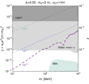
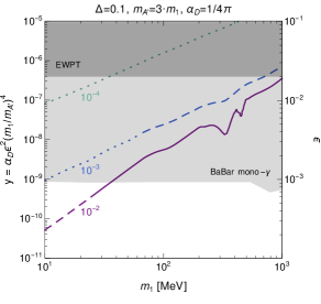
Figure 3: Collider bounds in the $(m_{1},y)$ plane of the i2DM. The dark gray area is excluded by electroweak precision observables bound of Eq. (53) while the light gray area is excluded by BaBar’s mono-photon search, see Sec. 5.3. The green area (BBN) is excluded for $\theta=10^{-4}$ due to late photodisintegration of light nuclei, see Sec. 4.2. Colored curves correspond to contours of $\Omega_{\chi}h^{2}=0.12$ for fixed values of $\tan\theta=10^{-2}$ (purple), $10^{-3}$ (blue) and $10^{-4}$ (green) for fixed relative mass splitting $\Delta=0.05$ (right) and 0.1 (left). On the curves, the three regions introduced in Sec. 3.2 are indicated as plain (A), dashed (B), and dotted (C).

5.4 Bounds from fixed-target experiments

Fixed-target experiments with a large separation of the particle source and the detector are particularly sensitive to particles with a long decay length. Searches for long-lived particles with sub-GeV masses have been performed at various fixed-target experiments and have been reinterpreted for iDM scenarios, for instance in Refs. Gninenko:2012eq ; Izaguirre:2017bqb ; Tsai:2019buq . In general, a beam of particles is dumped on a target material, producing light mesons such as pions or kaons. In iDM and i2DM, dark photons can be produced either in meson decays, through the Primakoff process or from bremsstrahlung. Subsequently the dark photons decay into pairs of dark fermions $\chi_{1}$ and/or $\chi_{2}$.

Depending on the model parameters, inelastic dark matter can be detected via three signatures: (displaced) decays of dark partners, $\chi_{2}\to\chi_{1}\ell^{+}\ell^{-}$; (up-)scattering of dark fermions off the detector material, $\chi_{i}N\to\chi_{j}N$; or missing energy from dark fermions that are stable at the scales of the experiment. The relative sensitivity to each signature depends on the lifetime of the dark partner, as well as on the experimental setup: short-lived dark partners are mostly observed through decays, while long-lived partners scatter inside the detector material or decay after passing through the detector. In what follows, we discuss the relevant signatures for i2DM and derive bounds from searches at fixed-target experiments.

Partner decays

For partner decays, the expected event rate in the far detector is given by

$$N_{\rm dec}\approx N_{A^{\prime}}\Big{(}\mathcal{B}(A^{\prime}\to\chi_{1}\chi_{2})+2\mathcal{B}(A^{\prime}\to\chi_{2}\chi_{2})\Big{)}\frac{1}{N_{2}}\sum_{k=1}^{N_{2}}\,P_{\rm dec}(d_{k})\,,$$ (56)

where $N_{A^{\prime}}\propto\epsilon^{2}$ is the total number of dark photons produced in a given experiment, and $N_{2}$ is the total number of $\chi_{2}$ states resulting from $N_{A^{\prime}}$ dark photon decays. The branching ratios are $\mathcal{B}(A^{\prime}\to\chi_{1}\chi_{2})\approx 1$ for iDM and $\mathcal{B}(A^{\prime}\to\chi_{2}\chi_{2})\approx 1$ for i2DM with $\tan\theta\ll 1$. Finally, $P_{\rm dec}(d_{k})$ is the probability to detect the decay products of particle $k$ with decay length $d_{k}$. The decay length $d_{k}=(\beta\gamma)_{k}c\tau_{2}$ depends on the boost, $(\beta\gamma)_{k}$, and on the lifetime, $\tau_{2}$, of the dark partner. For decay lengths longer than the baseline, the decay probability scales as $P_{\rm dec}(d)\propto 1/d$. In this regime, the expected event rates for iDM and i2DM depend on the model parameters as

$$N_{\rm dec}^{\rm iDM}\propto\epsilon^{2}y\propto\epsilon^{4}\alpha_{D}\,,\qquad N_{\rm dec}^{\rm i2DM}\approx 2\tan^{2}\theta\cos^{4}\theta\,N_{\rm dec}^{\rm iDM}\,.$$ (57)

In i2DM, the lifetime of the dark partner scales as $\tau_{2}\sim 1/\tan^{2}\theta$. For small $\tan\theta$, the dark partner tends to decay after passing the detector, which reduces the event rate. The factor of 2 accounts for the two dark partners produced in $A^{\prime}\to\chi_{2}\chi_{2}$ decays. For fixed parameters $\alpha_{D},\,m_{1},\,m_{A^{\prime}},\,\Delta$, a bound on $\epsilon$ obtained from searches for dark partner decays in iDM translates into a bound on $\epsilon\cdot(2\tan^{2}\theta\cos^{4}\theta)^{1/4}$ in i2DM.

Decays at CHARM

Strong bounds on long-lived dark particles decaying into electrons have been set at the neutrino experiment CHARM. At CHARM, dark fermions can be efficiently produced from $\pi^{0}$ or $\eta$ meson decays, $\pi^{0}(\eta)\to\gamma A^{\prime}\to\gamma\chi_{i}\chi_{j}$. Null results of a beam-dump search for heavy neutrinos decaying into electron pairs CHARM:1983ayi have been reinterpreted for $\chi_{2}\to\chi_{1}e^{+}e^{-}$ decays in iDM Tsai:2019buq . In Fig. 4, we show the resulting bounds in the parameter space of i2DM, using Eq. (57) to rescale the predicted event rates. The three scenarios are distinguished by the mass splitting $\Delta$, while we have fixed $\epsilon=10^{-3}$ to evade the collider bounds from Sec. 5.3.

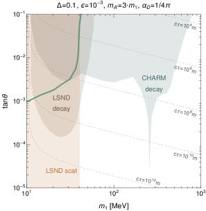
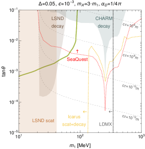
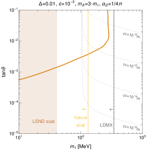
Figure 4: Bounds on i2DM from fixed-target experiments as a function of the dark fermion mixing $\theta$ and the dark matter mass $m_{1}$. Shown are three scenarios with a relative mass splitting $\Delta=0.1$, $0.05$, $0.01$, and fixed dark-photon mixing $\epsilon=10^{-3}$, dark-photon mass $m_{A^{\prime}}=3m_{1}$ and dark coupling strength $\alpha_{D}=1/(4\pi)$. The observed relic abundance is obtained along the colored contours. The dashed contours indicate the proper decay length of the dark partner. For $m_{1}<2m_{e}/\Delta$, the dark partner can only decay into photons or neutrinos, resulting in a very long lifetime. The bounds have been obtained by rescaling dedicated analyses for iDM. We show existing bounds from CHARM (grey areas) and LSND (red areas). The projected sensitivity of future experiments ICARUS (yellow), SeaQuest (red) and LDMX (grey) is illustrated by dotted lines; the arrow indicates the direction in parameter space that will be probed. All scenarios evade existing bounds from a mono-photon search at BaBar and electroweak precision tests (EWPT). See text for details.

The observed relic abundance is obtained along the colored contours. The lifetime of $\chi_{2}$ varies strongly with the mass splitting, $\tau_{2}\propto 1/\Delta^{5}$, see Eq. (14). For $\Delta=0.1$, most of the dark partners decay within the considered decay volume and the search is sensitive to even small mixing $\tan\theta$. For $\Delta=0.05$, the sensitivity decreases due to the longer lifetime and softer $e^{+}e^{-}$ momenta, which are less likely to pass the analysis cuts. For $\Delta=0.01$, the dark partner is essentially stable compared to the length of the decay volume and the search becomes insensitive to i2DM.

Decays at LSND

For light dark sectors, even stronger bounds have been obtained from the neutrino experiment LSND. At LSND, dark fermions can be abundantly produced from pion decays via $\pi^{0}\to\gamma A^{\prime}\to\gamma\chi_{i}\chi_{j}$. In Ref. Izaguirre:2017bqb , LSND data has been interpreted in terms of $\chi_{2}\to\chi_{1}e^{+}e^{-}$ decays in iDM, under the conservative assumption that the $e^{+}e^{-}$ pair is not resolved in the calorimeter and can mimic elastic neutrino-electron scattering. In Fig. 4, we show the resulting bounds rescaled for i2DM (labelled ‘LSND decay’). LSND is very sensitive to dark partners with $m_{2}<m_{\pi^{0}}/2$. The lower cutoff is determined by the kinematic threshold for $\chi_{2}\to\chi_{1}e^{+}e^{-}$ decays. The sensitivity could be improved with a dedicated analysis of three-body decays, rather than a re-interpretation of neutrino-electron scattering.

Dark fermion scattering

In addition to decays, long-lived dark fermions can be detected through up-scattering $\chi_{1}\to\chi_{2}$, down-scattering $\chi_{2}\to\chi_{1}$, or elastic scattering $\chi_{2}\to\chi_{2}$ inside the detector. We neglect up-scattering, which is typically sub-dominant for suppressed $\chi_{1}-\chi_{2}$ couplings. The expected scattering rate is then given by

$$N_{\rm scat}\approx N_{A^{\prime}}\Big{(}\mathcal{B}(A^{\prime}\to\chi_{1}\chi_{2})+2\mathcal{B}(A^{\prime}\to\chi_{2}\chi_{2})\Big{)}\frac{1}{N_{2}}\sum_{k=1}^{N_{2}}\,P_{\rm scat}(d_{k})\,,$$ (58)

where $P_{\rm scat}(d_{k})$ is the probability for particle $k$ to scatter off the material inside the detector, with $d_{k}\to\infty$ for $\chi=\chi_{1}$, and $N_{2}$ is the number of produced dark partners. Neutrino experiments are particularly sensitive to dark fermion scattering, which mimics neutrino-electron scattering. Among various experiments, LSND sets the currently strongest bounds on inelastic dark matter. For iDM and sub-GeV masses, the relevant process is down-scattering $\chi_{2}N\to\chi_{1}N$ Izaguirre:2017bqb . For i2DM, elastic scattering $\chi_{2}\to\chi_{2}$ dominates for $\tan\theta\ll 1$. The respective event rates scale as

$$N_{\rm scat}^{\rm iDM}\propto\epsilon^{4}\alpha_{D}\,,\qquad N_{\rm scat}^{\rm i2DM}\approx 2\cos^{4}\theta\,N_{\rm scat}^{\rm iDM}$$ (59)

for decay lengths $d_{k}$ larger than the distance between the target and the detector.

Scattering at LSND

The LSND bounds on scattering are derived from the same analysis as for partner decays. Again, we translate the results for iDM from Ref. Izaguirre:2017bqb to i2DM, shown in Fig. 4 as ‘LSND scat’. For $\tan\theta\lesssim 0.3$, the bounds are insensitive to dark fermion mixing and exclude small dark matter masses. The bounds disappear for small kinetic mixing $\epsilon\lesssim 10^{-4}$, where LSND loses its sensitivity due to the low dark photon production rate.

It is interesting to compare these results for i2DM with iDM. For $\tan\theta=1$, the $A^{\prime}\chi_{1}\chi_{2}$ interaction strength is similar in iDM and i2DM. For the benchmark scenarios shown in Fig. 4, iDM is excluded by CHARM and LSND, unless partner decays into electrons are kinematically forbidden. Viable scenarios of sub-GeV iDM require a stronger interaction strength $y$ for efficient coannihilation, while keeping the kinetic mixing $\epsilon$ small to evade bounds from mono-photon searches Batell:2021ooj , see Sec. 5.3. In turn, i2DM scenarios with small $\tan\theta$ can evade the CHARM bounds due to the longer lifetime of the dark partners. In this regime, the relic abundance is set by partner annihilation and/or coscattering. In summary, null searches at current fixed-target experiments are a severe challenge for iDM, while i2DM is a viable option due to the impact of partners on dark matter freeze-out.

5.5 Prospects of future fixed-target experiments

As we discussed in Sec. 5.4, existing fixed-target experiments are very sensitive to sub-GeV inelastic dark matter. However, in the multi-GeV range i2DM scenarios with a compressed dark sector currently escape detection. In order to fully explore the parameter space of i2DM, we study the discovery potential of proposed searches at fixed-target experiments, which could be realized in the near future. While a number of experiments can be sensitive to i2DM, here we focus a few promising proposals.

SBN

The Short-Baseline Neutrino (SBN) program at Fermilab Machado:2019oxb is a planned facility to probe neutrinos and light dark sectors. The facility uses the Booster 8 GeV proton beam hitting a beryllium target. Three detectors are placed downstream of the target at varying distances. The SBND detector is located at around 110 m, while the experiments MicroBooNE and ICARUS are placed further away, at 470 m and 600 m respectively.

At SBN, similarly to other fixed-target experiments discussed in Sec. 5.4, dark partners can be produced from decaying dark photons, which are created in the interaction of the proton beam with the target. The SBN detectors can be used to search for $\chi_{2}\to\chi_{1}\ell^{+}\ell^{-}$ decays or scattering $\chi_{i}\rightarrow\chi_{j}$ off the detector material.

Dark sector searches at neutrino experiments inevitably feature a large neutrino background. At SBN, there are two proposals to reduce this background. One option is to deflect the proton beam around the target into an iron absorber placed 50 m downstream, which has previously been done at MiniBooNE to study light dark sectors MiniBooNE:2017nqe ; MiniBooNEDM:2018cxm . This mode is referred to as “off-target”. The second option is to use the NuMI 120 GeV proton beam, impacting on a graphite target. ICARUS and MicroBooNE are placed at angles of 6 and 8 degrees against the NuMI beam direction. This option is known as “off-axis”. Both off-target and off-axis options have been studied for iDM Batell:2021ooj , where SBND has the best sensitivity in the off-target mode, while ICARUS can set the strongest bound in the off-axis mode. In Fig. 4, we show our reinterpretation of these predictions for i2DM, following the procedure described in Sec. 5.4. We present the results for ICARUS, assuming that the off-axis mode can be realized with much less technological effort than the off-target option. Compared to existing fixed-target experiments, ICARUS is substantially more sensitive to i2DM, provided that the dark partners are sufficiently long-lived to induce enough signal in the detector.

SeaQuest

Originally developed to study the sea quark content of the proton with a 120 GeV proton beam and various targets, the Fermilab experiment SeaQuest has a good potential to probe dark sectors Gardner:2015wea ; Berlin:2018pwi . It is already equipped with a displaced muon trigger to study exotic long-lived particles decaying to muons, and could be supplemented by an electromagnetic calorimeter to also probe electron signals. In Ref. Berlin:2018pwi , the sensitivity of SeaQuest to dark partner decays in iDM has been studied for three different decay volumes. In Fig. 4, we show the corresponding predictions for i2DM for the largest possible decay volume. Compared with CHARM and ICARUS, SeaQuest can improve the sensitivity to i2DM for dark matter with masses near the $\eta$ resonance. As discussed in Ref. Berlin:2018pwi , the reach of SeaQuest could be further enhanced by running the experiment without the magnet, which however would require a dedicated analysis of the experimental setup.

LDMX

The proposed Light Dark Matter eXperiment (LDMX) LDMX:2018cma is an electron beam-dump experiment designed primarily for probing light dark matter models. Its search strategy relies on dark sector particles being produced in the beam dump that escape the detector, which extends up to about $1\,$m downstream from the target. This gives rise to a signature of missing energy. All charged particles in an event are vetoed, except for the soft remnant of the incoming electron. A signal of inelastic dark matter is detected if a substantial fraction of dark partners decay after passing through the detector. The LDMX collaboration has investigated the projected sensitivity to many MeV-GeV dark sector models, including iDM Berlin:2018bsc . In Fig. 4, we show our interpretation for i2DM for the most conservative design option. LDMX is well suited to probe i2DM scenarios with very small mass splitting $\Delta$, which are difficult to detect in experiments that detect the decay products of the dark partner.

We summarize our projections for future fixed-target experiments for the three i2DM benchmarks in Fig. 4. For $\Delta=0.1$, the dark matter target is already probed by existing experiments. We therefore do not show projections for future experiments, but note that they could be sensitive to other regions of the parameter space. For $\Delta=0.05$, SeaQuest alone can improve the sensitivity to dark partner decays, but cannot fully probe the dark matter target. ICARUS can complement SeaQuest by also detecting dark fermion scattering, which is predominant for small dark matter masses. LDMX, searching for missing energy, can extend the reach of ICARUS at larger masses and long lifetimes. Either ICARUS or LDMX could conclusively probe this scenario. For even smaller mass splitting $\Delta=0.01$, dark partner decays cannot be observed due to the long lifetime and the softness of the SM decay products. The sensitivity of ICARUS and LDMX through scattering and missing energy, however, is kept and allows to conclusively probe the dark matter scenario. Larger dark photon masses $m_{A^{\prime}}>3m_{1}$ or smaller kinetic mixing $\epsilon$ reduces the rate of produced dark photons and thus the sensitivity of any experiment. For smaller dark couplings $\alpha_{D}$, the lifetime of the dark partners is enhanced and dark partner decays close behind the target are less abundant. In this case, scattering and missing energy are more promising signals, especially for small dark matter masses. All in all, fixed-target experiments have a high potential to conclusively test i2DM in the near future, provided that they are built and successfully run.

6 Conclusions and outlook

In this work we have introduced a new model for feebly coupling dark matter, called inelastic Dirac Dark Matter. Compared to the widely studied model of inelastic Dark Matter with Majorana fermions, i2DM has a different thermal history and is less constrained by current laboratory searches. The main difference is due to the variable interaction strength of the dark matter candidate $\chi_{1}$, parametrized by a mass mixing $\theta$ with its dark partner $\chi_{2}$.

At small mass mixing, the dark matter candidate decouples from the SM bath before freeze-out and the relic dark matter abundance cannot be set by dark matter annihilation, coannihilation or partner annihilation anymore. Instead, coscattering and decay processes are crucial to explain the observed abundance even for tiny dark matter interactions $y$ with the thermal bath. At such feeble couplings, dark matter can decouple from chemical and even kinetic equilibrium before freeze-out. We have computed the resulting effects on the relic abundance by numerically solving a coupled set of Boltzmann equations for the time evolution of the dark fermions. For particles in the multi-MeV range, we find that the relic abundance can be obtained with interactions as feeble as $y\gtrsim 10^{-11}$ and is only mildly affect by deviations from kinetic equilibrium.

Requesting that the QCD phase transition should not affect the freeze-out dynamics and that $\Delta N_{\rm eff}$ contributions for i2DM is in agreement with CMB data be suppressed, we identify the cosmologically viable parameter region for i2DM candidates with mass and interaction strength in the range

$$10\,\text{MeV}<m_{1}<1\,\text{GeV}\,,\quad y>10^{-11}.$$ (60)

In this region, we have investigated possible effects of i2DM on Big Bang Nucleosynthesis, the Cosmic Microwave Background and supernova cooling, but find them much too small to modify current observations.

Laboratory searches for i2DM mostly rely on the production of dark photons, subsequently decaying into dark fermions. Due to the feeble interaction, the dark partner typically appears stable at the scales of current colliders. Searches for mono-photons and missing momentum at flavor experiments set a strong bound on the overall coupling of the dark photon to the Standard Model, $\epsilon\lesssim 10^{-3}$. These bounds imply a minimum dark fermion mixing and require efficient partner annihilation to satisfy the relic abundance. The parameter range for viable i2DM is thereby confined to light and compressed dark sectors with

$$10\,\text{MeV}<m_{1}<200\,\text{MeV}\,,\quad\Delta<0.1\,,\quad\epsilon<10^{-3}\,.$$ (61)

At direct detection experiments, $\chi_{1}N\to\chi_{2}N$ up-scattering off atomic nuclei is not efficient enough to further test i2DM, even if dark matter can be accelerated through interactions with cosmic rays. On the other hand, long-lived dark partners can be produced in cosmic-ray up-scattering might leave an observable signature of $\chi_{2}N\to\chi_{2}N$ elastic scattering in the detector material. We leave this interesting avenue for future work.

Very promising probes of i2DM are fixed-target experiments with a long baseline, which can search for decays or scattering of long-lived dark partners in far detectors. Scattering is a prominent signal for light dark partners, while decays can be observed for heavier partners up to the GeV scale. Current searches for such signatures at CHARM and LSND already probe a significant portion of the i2DM parameter space, but lose steam for small mass splitting, where the momentum deposit in the detector is soft.

In the near future, neutrino experiments like ICARUS and SeaQuest or the beam-dump experiment LDMX can significantly improve the sensitivity to inelastic dark matter. Together with mono-photon searches at Belle II, they can conclusively test if inelastic Dirac dark matter is at the origin of the observed relic abundance.

Acknowledgments

We thank Alberto Mariotti for many interesting discussions and for contributions at an early stage of this work. We also thank Jan Heisig and Matteo Lucca for helpful discussions and Marco Hufnagel for support with ACROPOLIS and exchanges. The research of AF was supported by the NWO Vidi grant “Self-interacting asymmetric dark matter”. LLH is a research associate of the Fonds de la Recherche Scientifique F.R.S.-FNRS. LLH and SJ have been supported by the FNRS research grant number F.4520.19 and the IISN convention 4.4503.15. LLH also acknowledges support of the ARC program of the Federation Wallonie-Bruxelles. SJ is further supported by the Université Libre de Bruxelles PhD grant and the Strategic Research Program High-Energy Physics and the Research Council of the Vrije Universiteit Brussel. The research of SW has been supported by the German Research Foundation (DFG) under grant no. 396021762–TRR 257.

Appendix A Formalism of i2DM

We provide further details about inelastic Dirac dark matter introduced in Sec. 2. The interactions of mass eigenstates described by the Lagrangian from Eq. (1) can be derived from gauge-invariant interactions of the dark sector with the Standard Model in the unbroken phase of the underlying theory,

$$\mathcal{L}= \ i\,\bar{\chi}_{D}\gamma^{\mu}D_{\mu}\chi_{D}-m_{D}\bar{\chi}_{D}\chi_{D}+i\,\bar{\chi}_{0}\gamma^{\mu}\partial_{\mu}\chi_{0}-m_{0}\bar{\chi}_{0}\chi_{0}$$ (62)

$$\qquad+(D^{\mu}\phi_{D})^{\dagger}(D_{\mu}\phi_{D})+V(\phi_{D})-(\lambda\phi_{D}\bar{\chi}_{D}\chi_{0}+h.c.)$$

$$\qquad-\frac{1}{4}\hat{F}_{D\mu\nu}\hat{F}_{D}^{\mu\nu}-\frac{1}{2}\frac{\epsilon}{c_{W}}\hat{B}_{\mu\nu}\hat{F}_{D}^{\mu\nu},$$

Here $D_{\mu}=\partial_{\mu}+ig_{D}Q_{D}\hat{A}_{D\mu}$ is the covariant derivative for the gauge field $\hat{A}_{D}$ of the dark $U(1)_{D}$ symmetry. The field strength tensors for the dark and the hypercharge gauge fields are denoted as $\hat{F}_{D}^{\mu\nu}$ and $\hat{B}^{\mu\nu}$ respectively. The dark fermion field $\chi_{D}$ is charged under $U(1)_{D}$, while $\chi_{0}$ is a singlet under all gauge interactions.

The scalar $\phi_{D}$ with potential $V(\phi_{D})$ and charge $Q_{D}=1$ facilitates spontaneous $U(1)_{D}$ breaking, once it develops a vacuum expectation value $v_{D}$, so that $\phi_{D}=(v_{D}+\varphi_{D})/\sqrt{2}$. Upon symmetry breaking, the dark photon $\hat{A}_{D}$ acquires a mass $m_{\hat{A}_{D}}=g_{D}v_{D}$, and the dark fermions $\chi_{D}$ and $\chi_{0}$ mix through the dark Yukawa coupling $\lambda$, resulting in two mass eigenstates

$$\begin{pmatrix}\chi_{1}\\ \chi_{2}\end{pmatrix}=\begin{pmatrix}\cos\theta&-\sin\theta\\ \sin\theta&\cos\theta\end{pmatrix}\begin{pmatrix}\chi_{0}\\ \chi_{D}\end{pmatrix},\qquad\sin(2\theta)=\frac{\sqrt{2}\lambda v_{D}}{\Delta m_{1}}\,.$$ (63)

The corresponding masses are

$$m_{1,2}=\frac{1}{2}\big{(}m_{D}+m_{0}\pm\Delta m_{1}\big{)}\quad{\rm with}\quad(\Delta m_{1})^{2}=(m_{D}-m_{0})^{2}+2(\lambda v_{D})^{2}\,,$$ (64)

where $\Delta$ is the relative mass difference defined in Eq. (4). In order to obtain canonical kinetic terms in Eq. (62), we first redefine the $U(1)_{Y}$ and $U(1)_{D}$ gauge bosons to absorb the kinetic mixing via

$$\begin{pmatrix}\hat{B}^{\mu}\\ \hat{A}^{\mu}_{D}\end{pmatrix}=G(\hat{\epsilon})\begin{pmatrix}\tilde{B}^{\mu}\\ \tilde{A}^{\mu}_{D}\end{pmatrix}=\begin{pmatrix}1&&-\frac{\hat{\epsilon}}{\sqrt{1-\hat{\epsilon}^{2}}}\\ 0&&\frac{1}{\sqrt{1-\hat{\epsilon}^{2}}}\end{pmatrix}\begin{pmatrix}\tilde{B}^{\mu}\\ \tilde{A}^{\mu}_{D}\end{pmatrix},$$ (65)

where $\hat{\epsilon}=\epsilon/\cos\theta_{W}$. Subsequently, we transform the fields to the physical eigenstates of weak interactions, $A^{\mu},\,Z^{\mu},\,A^{\prime\mu}$, via two rotations: one rotation, $R_{\xi}$, mixing the $SU(2)$ gauge field $W^{3}_{\mu}$ and $\tilde{A}^{\mu}_{D}$ with an angle $\xi$; and a second rotation, $R_{W}$, mixing $W^{3}_{\mu}$ and $\tilde{B}_{\mu}$ with the Weinberg angle $\theta_{W}$. The overall transformation takes the form

$$\begin{pmatrix}\tilde{B}^{\mu}\\ W^{3\mu}\\ \tilde{A}^{\mu}_{D}\end{pmatrix}=\begin{pmatrix}c_{W}&&-c_{\xi}s_{W}&&s_{\xi}s_{W}\\ s_{W}&&c_{\xi}c_{W}&&-s_{\xi}c_{W}\\ 0&&s_{\xi}&&c_{\xi}\end{pmatrix}\,\begin{pmatrix}A^{\mu}\\ Z^{\mu}\\ A^{\prime\mu}\end{pmatrix},$$ (66)

where

$$\tan 2\xi=\frac{2\eta s_{W}}{1-(\eta s_{W})^{2}-\delta}$$ (67)

$${\rm with}\quad\eta=\hat{\epsilon}/\sqrt{1-\hat{\epsilon}^{2}},\quad\delta=\hat{\delta}/(1-\hat{\epsilon}^{2}),\quad\hat{\delta}=m_{\hat{A}_{D}}^{2}/m_{\hat{Z}}^{2}\,,$$

and $m_{\hat{Z}}=gv/(2c_{W})$, with the $SU(2)$ gauge coupling, $g$, and the SM Higgs vacuum expectation value, $v$. The masses of the $Z$ boson and the dark photon are

$$m^{2}_{Z}=m_{\hat{Z}}^{2}\left((c_{\xi}+\eta s_{\xi}s_{W})^{2}+s_{\xi}^{2}\delta\right)\quad{\rm and}\quad m^{2}_{A^{\prime}}=m_{\hat{Z}}^{2}\left((-s_{\xi}+c_{\xi}\eta s_{W})^{2}+c_{\xi}^{2}\delta\right),$$ (68)

while the photon remains massless. In the limit of small kinetic mixing, $\{\epsilon,\eta,\xi\}\ll 1$, one recovers $m_{Z}\simeq m_{\hat{Z}}$ and $m_{A^{\prime}}\simeq m_{\hat{A}_{D}}$ Wells:2008xg ; Curtin:2014cca ; Freitas:2015hsa ; Foldenauer:2019vgn .

To derive the Feynman rules and transition amplitudes, we use FeynRules Alloul:2013bka . In particular, we have adapted the Hidden Abelian Higgs Model Wells:2008xg , which is available from the FeynRules model data base to i2DM. Our FeynRules model for i2DM is available at FeynRulesModel . In terms of mass eigenstates, the Lagrangian finally reads

$$\mathcal{L}\supset \ -e\big{(}A_{\mu}-\epsilon A^{\prime}_{\mu}\big{)}J^{\mu}_{em}+\frac{e}{2s_{W}c_{W}}Z_{\mu}J^{\mu}_{Z}$$ (69)

$$-g_{D}\left(A^{\prime}_{\mu}+\epsilon\,t_{W}Z_{\mu}\right)\big{(}s_{\theta}^{2}J^{\mu}_{1}+c_{\theta}^{2}J^{\mu}_{2}-c_{\theta}s_{\theta}J^{\mu}_{12}\big{)}$$

$$-\frac{\lambda}{\sqrt{2}}\varphi_{D}\big{(}c_{2\theta}(\bar{\chi}_{1}\chi_{2}+\bar{\chi}_{2}\chi_{1})-s_{2\theta}(\bar{\chi}_{1}\chi_{1}-\bar{\chi}_{2}\chi_{2})\big{)}$$

$$+\frac{g_{D}^{2}}{2}\big{(}2v_{D}\varphi_{D}+\varphi_{D}^{2}\big{)}\big{(}A^{\prime}_{\mu}A^{\prime\mu}+\epsilon\,t_{W}(A^{\prime}_{\mu}Z^{\mu}+Z_{\mu}A^{\prime\mu})+\epsilon^{2}t_{W}^{2}Z_{\mu}Z^{\mu}\big{)}\,,$$

where $t_{W}$ refers to the tangent of the Weinberg angle $\theta_{W}$. The dark currents $J^{\mu}_{i}$ with $(i=1,2)$ and $J^{\mu}_{12}$ are defined in Eq. (2). The SM fermion currents are given by

$$J^{\mu}_{Z}=\bar{f}(c_{V}\gamma^{\mu}-c_{A}\gamma^{\mu}\gamma^{5})f,\quad J^{\mu}_{em}=Q_{f}\bar{f}\gamma^{\mu}f,$$ (70)

where $f$ are the SM fermions and $c_{V}=T_{f}^{3}-2s_{W}^{2}Q_{f}$, $c_{A}=T_{f}^{3}$ are the electroweak charges, with $T_{f}^{3}$ the weak isospin quantum number and $Q_{f}$ the electric charge in units of $e$. Here we have only included the leading terms in $\epsilon$ and provided the SM fermion couplings in unitary gauge.

From the transformations of Eqs. (65) and (66) and the Lagrangian in Eq. (69), it should be clear that the photon $A^{\mu}$ has no field component from the dark $U(1)_{D}$ gauge field $\hat{A}^{\mu}_{D}$. As a result, the photon has no fundamental couplings to the dark fermions $\chi_{1},\,\chi_{2}$. In particular, the dark matter candidate $\chi_{1}$ carries no millicharge and is not subject to otherwise strong constraints Hambye:2019dwd .

Appendix B Boltzmann equations beyond thermal equilibrium

On general grounds, in an isotropic and homogeneous universe the evolution of a particle species $i$ is described in terms of a distribution function $f_{i}(t,|\vec{p}_{i}|)$, expressed in terms of the physical time $t$ and of the norm of the physical 3-momentum $\vec{p}_{i}$, denoted as $|\vec{p}_{i}|\equiv p_{i}$. If a species $i$ interacts with other species $j$, the time evolution of species $i$ is described by the Boltzmann equation

$$\frac{df_{i}(t,p_{i})}{dt}=\frac{1}{E_{i}}\,{\cal C}[f_{i}(t,p_{i}),f_{j}(t,p_{j})]\,,$$ (71)

where ${\cal C}[f_{i}(t,p_{i}),f_{j}(t,p_{j})]$ is the collision term involving all decay and scattering processes with the other species $j$, and $E_{i}=\sqrt{p_{i}^{2}+m_{i}^{2}}$ is the energy of particles of species $i$ with mass $m_{i}$. In this appendix, and in particular in Sec. B.2, we give more details about the collision terms for coscattering, ${\cal C}_{\rm coscat}$, and 3-body inverse decays, ${\cal C}_{\rm decay}$.

The total time derivative in Eq. (71) can be re-expressed in terms of partial derivatives with respect to time and momentum as

$$\frac{df_{i}(t,p_{i})}{dt} = \left(\partial_{t}-Hp_{i}\partial_{p_{i}}\right)f_{i}(t,p_{i})=\overline{H}\left(x\partial_{x}+\frac{x}{3h_{\rm eff}}\frac{dh_{\rm eff}}{dx}\,q_{i}\,\partial_{q_{i}}\right)f_{i}(x,q_{i}),$$ (72)

with

$$\overline{H}=H\left(1-\frac{x}{3h_{\rm eff}}\frac{dh_{\rm eff}}{dx}\right)^{-1}.$$ (73)

In Eq. (72) we have used the rescaled time $x$ and momentum variable $q_{i}$ introduced in Eq. (18). In this appendix, we will make use of the variables $(t,p_{i})$ or $(x,q_{i})$ whenever convenient. Also, $H=H(x)$ is the Hubble expansion rate and $h_{\rm eff}=h_{\rm eff}(x)$ is the effective number of relativistic degrees of freedom contributing to the entropy density $s=h_{\rm eff}\,{2\pi^{2}}/45\,T^{3}$. In this paper we consider dark matter production in a radiation dominated era, in which case the Hubble rate reduces to

$$H(x) = \frac{m_{1}^{2}}{x^{2}M_{0}}\quad{\rm with}\quad M_{0}=M_{P}\sqrt{\frac{45}{4\pi^{3}g_{*}}}\,,$$ (74)

where $M_{P}$ is the Planck mass and $g_{\ast}=g_{\ast}(x)$ denotes the number of relativistic degrees of freedom in the thermal bath at time $x$ contributing to the radiation energy density $\rho_{R}=g_{\ast}\,\pi^{2}/30\,T^{4}$. For our numerical analysis, we use tables available in the public code micrOMEGAs Belanger:2018ccd to evaluate $h_{\rm eff}(x)$ and $g_{\ast}(x)$. When the number of relativistic degrees of freedom, $h_{\rm eff}$ and $g_{\ast}$, can be considered constant around freeze-out, the unintegrated Boltzmann equations of Eq. (72) simplify to

$$xH\,\partial_{x}f_{i}(x,q_{i})=\frac{1}{E_{i}}{\cal C}[f_{i}(x,q_{i}),f_{j}(x,q_{j})]\,,$$ (75)

as reported in Eq. (23). To compute the dark matter freeze-out beyond kinetic and chemical equilibrium in i2DM, we will use the latter evolution equation, see Sec. B.2 for details.

In what follows, we will encounter the equilibrium number densities $n^{i}_{\text{eq}}(t)$, i.e., the number densities obtained by integrating over the kinetic equilibrium distribution functions $f^{\rm eq}_{i}(t,p_{i})$, where $f^{\rm eq}_{i}(t,p_{i})$ are the Fermi-Dirac, Bose-Einstein or Boltzmann distributions for zero chemical potential.

B.1 Deviation from chemical equilibrium before freeze-out

In i2DM, as long as deviations of $\chi_{1}$ from kinetic equilibrium with the heat bath can be neglected up until freeze-out, the evolution of $\chi_{1,2}$ can be described by the number densities $n_{1,2}(x)$, or equivalently by the comoving number densities $Y_{1,2}(x)$. Within this framework, it is useful to introduce the reaction densities for decays and scattering,

$$\gamma_{i\to jkl} = \int d\phi_{i}\phi_{j}d\phi_{k}d\phi_{l}f_{i}^{\rm eq}(t,p_{i})(2\pi)^{4}\delta^{4}(p_{i}-p_{j}-p_{k}-p_{l})|{\cal M}_{i\to jkl}|^{2}$$ (76)

$$\gamma_{ij\to kl} = \int d\phi_{i}d\phi_{j}f_{i}^{\rm eq}(t,p_{i})f_{j}^{\rm eq}(t,p_{j})\int d\phi_{k}d\phi_{l}(2\pi)^{4}\delta^{4}(p_{i}+p_{j}-p_{k}-p_{l})|{\cal M}_{ij\to kl}|^{2}\,,$$

which can be rewritten in terms of the thermally averaged cross section and the decay rate in the rest frame of species $i$, as in Eq. (26). In Eq. (76), $|{\cal M}|^{2}$ is the squared scattering amplitude, averaged over initial- and final-state degrees of freedom, and $d\phi_{i}=g_{i}d^{3}p_{i}/(2E_{i}(2\pi)^{3})$ denotes the phase-space element.

As long as $\chi_{1,2}$ can be assumed to be in kinetic and chemical equilibrium before freeze-out, the set of partial integro-differential equations for the dark fermions from Eq. (71), integrated over the 3-momenta $p_{i}$, reduces to one single well-known ordinary differential equation for the total dark sector number density $n(t)=\sum_{i=1,2}n_{i}(t)$ Griest:1990kh ; Gondolo:1990dk . This simplification applies to freeze-out in the phases of coannihilation and partner annihilation in region (A). In this regime, one can compute the dark matter relic abundance with any publicly available Boltzmann solver, such as micrOMEGAs Belanger:2018ccd , DarkSUSY Bringmann:2018lay or MadDM Ambrogi:2018jqj .

In the conversion phase, the very small interaction strength $y$ implies strongly suppressed coscatterings and decays and chemical equilibrium between $\chi_{1}$ and $\chi_{2}$ is lost. As a result, the relation $n_{1}/n_{2}=n_{1}^{\rm eq}/n_{2}^{\rm eq}$ cannot be assumed. In order to take deviations from chemical equilibrium into account, we have to solve a coupled system of Boltzmann equations including the conversion rates $\gamma_{1\to 2}$ Garny:2017rxs ; Garny:2018icg ; DAgnolo:2018wcn ; Junius:2019dci ; Herms:2021fql ,

$$\frac{dY_{1}}{dx}=\frac{-1}{\overline{H}xs} \left[\gamma_{11}\left(\frac{Y^{2}_{1}}{{Y_{1}^{\rm eq}}^{2}}-1\right)+\gamma_{12}\left(\frac{Y_{1}Y_{2}}{Y_{1}^{\rm eq}Y_{2}^{\rm eq}}-1\right)-\gamma_{2\to 1}\left(\frac{Y_{2}}{Y_{2}^{\rm eq}}-\frac{Y_{1}}{Y_{1}^{\rm eq}}\right)\right]$$ (77)

$$\frac{dY_{2}}{dx}=\frac{-1}{\overline{H}xs} \left[\gamma_{22}\left(\frac{Y^{2}_{2}}{{Y_{2}^{\rm eq}}^{2}}-1\right)+\gamma_{12}\left(\frac{Y_{1}Y_{2}}{Y_{1}^{\rm eq}Y_{2}^{\rm eq}}-1\right)+\gamma_{2\to 1}\left(\frac{Y_{2}}{Y_{2}^{\rm eq}}-\frac{Y_{1}}{Y_{1}^{\rm eq}}\right)\right],$$

where $\gamma_{ij}$ are the reaction densities defined in Eq. (28) and $\gamma_{i\to j}=\gamma_{i\to j}^{dec}+\gamma_{i\to j}^{scat}$. For i2DM, we have checked that we can neglect quantum statistical effects in the relevant density distributions $f_{i}$ and use the Maxwell-Boltzmann equilibrium distributions $f_{i}^{\rm eq}$. In i2DM, Eq. (77) can safely be used for freeze-out scenarios in regions (A) and (B), where kinetic equilibrium is maintained up to freeze-out.

B.2 Deviation from chemical and kinetic equilibrium around freeze-out

When the conversion rate is around 10 to 100 times the Hubble rate at the time of $\chi_{2}$ chemical decoupling, dark matter can no longer be expected to be kept in chemical or kinetic equilibrium with $\chi_{2}$ around the DM freeze-out time $x_{\rm fo}$. The assumptions for Eq. (77) do not hold anymore, and a priori one needs to solve Eq. (75) including the full momentum and time dependentce in the $\chi_{1}$ distribution function $f_{1}(x,q_{1})$.

For i2DM, we apply two levels of simplification to Eq. (75). First, we neglect the time dependence in $h_{\rm eff}$ for the dark matter density evolution, setting $h_{\rm eff}=h_{\rm eff}(x_{\rm fo})$ when integrating over $f_{1}(x,q_{1})$. For dark fermions in the MeV-GeV mass range, we obtain a good approximation to the exact solution of Eq. (75). In this mass range, freeze-out is expected to happen between the QCD phase transition and neutrino decoupling, a period in which $h_{\rm eff}\simeq 10.75$ is fairly constant. Second, we follow Refs. DAgnolo:2017dbv ; Garny:2017rxs and only take into account the dominant interaction processes driving the dark matter distribution $f_{1}(x,q_{1})$ towards kinetic equilibrium. For i2DM, this means that we include conversion processes but neglect coannihilation.

With these simplifications, the unintegrated Boltzmann equation for $f_{1}(x,q_{1})$ from Eq. (75) can be rewritten as

$$Hx\partial_{x}f_{1}(x,q) = \tilde{C}_{1\to 2}(x,q)\left(f_{1}^{\rm eq}(x,q)\frac{Y_{2}(x)}{Y_{2}^{\rm eq}(x)}-f_{1}(x,q)\right),$$ (78)

where $q=q_{1}=p_{1}/T$ to simplify the notation. The contributions to the collision operator $\tilde{C}_{1\to 2}(x,q)=\tilde{C}_{\rm coscat}(x,q)+\tilde{C}_{\rm decay}(x,q)$ from coscattering and decays are spelled out in Secs. B.2.1 and B.2.2. The above description assumes that $\chi_{2}$ and the light SM fermions involved in the conversion processes are in kinetic equilibrium. We also neglect all spin statistics effect.

The differential equation in Eq. (78) can be solved iteratively with $Y_{2}(x)$ as an input. The latter is obtained from the integrated Boltzmann equation for $Y_{2}$ in Eq. (77), which in turn involves $Y_{1}(x)$, or equivalently the zeroth moment of $f_{1}(x,q)$ in $q$, obtained by integrating over Eq. (78). More details on the integration of Eq. (78) will be discussed in Sec. B.2.3.

B.2.1 Coscattering

Here we provide details on the collision term due to coscattering. First we show that the collision term for coscatterings $\chi_{1}f\rightarrow\chi_{2}f^{\prime}$ can indeed be written as in Eq. (78). Neglecting spin-statistic effects, the collision term takes the form

$${\cal C}_{\text{coscat}}=\frac{1}{2}\int d\phi_{f}d\phi_{2}d\phi_{f^{\prime}}(2\pi)^{4}\delta^{(4)}(p_{1}+p_{f}-p_{2}-p^{\prime}_{f})|{\cal M}_{\chi_{1}f\rightarrow\chi_{2}f^{\prime}}|^{2}\left(f_{2}f_{f^{\prime}}-f_{1}f_{f}\right).$$ (79)

Assuming that the SM fermions $f$ and $f^{\prime}$ are in chemical and kinetic equilibrium with the thermal bath and that $\chi_{2}$ is in kinetic equilibrium throughout the $\chi_{1}$ freeze-out, we have $f_{x}(t,p_{k})=f^{\rm eq}_{k}(t,p_{k})$ for $k=\{f,f^{\prime}\}$ and $f_{2}(t,p_{2})=f_{2}^{\rm eq}(t,p_{2})\,Y_{2}(t)/Y_{2}^{\rm eq}(t)$, so that

$$f_{2}f_{f^{\prime}}-f_{1}f_{f}=\left(f_{2}^{\rm eq}\frac{Y_{2}}{Y_{2}^{\rm eq}}f_{f^{\prime}}^{\rm eq}-f_{1}f_{f}^{\rm eq}\right)=f_{f}^{\rm eq}\left(f_{1}^{\rm eq}\frac{Y_{2}}{Y_{2}^{\rm eq}}-f_{1}\right).$$ (80)

In the second equation we have used the relation of detailed balance, $f_{2}^{\rm eq}f_{f^{\prime}}^{\rm eq}=f_{1}^{\rm eq}f_{f}^{\rm eq}$. With Eq. (80), we can write the collision term as

$$\frac{1}{E_{1}}\,{\cal C}_{\text{coscat}}=\tilde{\cal C}_{\text{coscat}}\left(f_{1}^{\rm eq}\frac{Y_{2}}{Y_{2}^{\rm eq}}-f_{1}\right),$$ (81)

with the coscattering collision operator

$$\tilde{\cal C}_{\text{coscat}} = \frac{g_{f}T}{16\pi^{2}p_{1}E_{1}}\int ds\,\sigma_{\text{coscat}}(s)\,(s-m_{1}^{2})\left(e^{-E_{f}^{-}/T}-e^{-E_{f}^{+}/T}\right).$$ (82)

Here the cross section for coscattering process is defined as DAgnolo:2018wcn ; Garny:2018icg

$$\sigma_{\text{coscat}}(s)=\frac{1}{4\hat{p}_{1}\sqrt{s}}\int d\phi_{2}d\phi_{f^{\prime}}\ (2\pi)^{4}\delta^{4}(p_{1}+p_{f}-p_{2}-p^{\prime}_{f})\ |{\cal M}_{\chi_{1}f\rightarrow\chi_{2}f^{\prime}}|^{2}\,,$$ (83)

with the modulus of the dark matter 3-momentum in the centre-of-mass frame, $\hat{p}_{1}$, the squared center-of-mass energy, $s$, and the energy variables

$$E_{f}^{\pm}=\frac{s-m_{1}^{2}}{2m_{1}^{2}}(E_{1}\pm p_{1})\,.$$ (84)

B.2.2 Three-body decays

As mentioned in Sec. 3.1, the inverse decay process $\chi_{1}ff^{\prime}\to\chi_{2}$ can play a role in keeping $\chi_{1}$ in kinetic equilibrium. The corresponding collision reads

$${\cal C}_{\text{decay}}=\frac{1}{2}\int\!d\phi_{2}d\phi_{f}d\phi_{f^{\prime}}(2\pi)^{4}\delta^{(4)}(p_{2}-p_{1}-p_{f}-p^{\prime}_{f})|{\cal M}_{\chi_{2}\to\chi_{1}ff^{\prime}}|^{2}\left(f_{2}-f_{1}f_{f}f_{f^{\prime}}\right).$$ (85)

Assuming again that all involved SM fermions $f,f^{\prime}$ are in chemical and kinetic equilibrium with the thermal bath and that $\chi_{2}$ is in kinetic equilibrium with the bath, the collision term reduces to

$$\frac{1}{E_{1}}{\cal C}_{\text{decay}}=\tilde{\cal C}_{\text{decay}}\left(f_{1}^{\rm eq}\frac{n_{2}}{n_{2}^{\rm eq}}-f_{1}\right),$$ (86)

with the collision operator for decays,

$$\tilde{\cal C}_{\text{decay}} = \frac{g_{f^{\prime}}}{2E_{1}}\int d\phi_{2}d\phi_{f}\frac{2\pi}{2E^{\prime}_{f}}\delta(E_{2}-E_{1}-E_{f}-E^{\prime}_{f})|{\cal M}_{\chi_{2}\to\chi_{1}ff^{\prime}}|^{2}f_{f}^{\rm eq}f_{f^{\prime}}^{\rm eq}$$ (87)

after integrating over $d\phi_{f^{\prime}}$.

Applying the methodology from DEramo:2020gpr for 3-body decays and neglecting the SM fermion masses, the collision operator can be rewritten as

$$\tilde{\cal C}_{\text{decay}}=\frac{g_{f}g_{f^{\prime}}g_{2}}{256\pi^{3}p_{1}E_{1}} \int_{0}^{(\Delta m_{1})^{2}}\!\!\!\!\frac{dm_{ff^{\prime}}^{2}}{\sqrt{\lambda(m_{ff^{\prime}},m_{2},m_{1})}}$$ (88)

$$\times\int_{E_{2}^{-}}^{E_{2}^{+}}dE_{2}\,f_{f}^{\rm eq}f_{f^{\prime}}^{\rm eq}\int_{(m_{1f}^{2})^{-}}^{(m_{1f}^{2})^{+}}dm_{1f}^{2}|{\cal M}_{\chi_{2}\to\chi_{1}ff^{\prime}}|^{2},$$

where

$$\lambda(x,y,z) = (x^{2}-(y+z)^{2})(x^{2}-(y-z)^{2}),$$ (89)

$$m_{1f}^{2} = (p_{1}+p_{f})^{2},$$

$$m_{ff^{\prime}}^{2} = (p_{2}-p_{1})^{2}.$$

The integration boundaries are

$$E_{2}^{\pm} =\sqrt{m_{2}^{2}+(p_{2}^{\pm})^{2}},\quad{\rm with}$$

$$p_{2}^{\pm} =\frac{p_{1}(m_{1}^{2}+m_{2}^{2}-m_{ff^{\prime}}^{2})\pm\sqrt{(m_{ff^{\prime}}^{2}+m_{1}^{2})\lambda(m_{ff^{\prime}},m_{2},m_{1})}}{2m_{1}^{2}},$$

and $(m_{1f}^{2})^{\pm}=m_{1}^{2}+m_{ff^{\prime}}(\hat{E}_{1}\pm\hat{p}_{1})$, where the hatted quantities are evaluated in the reference frame where $\vec{p}_{f}=\vec{p}_{f^{\prime}}$.

B.2.3 Simplified unintegrated Boltzmann equation

The collision terms for inverse decays and coscattering from Eqs. (81) and (86) have the same form as the right-hand side of the simplified Boltzmann equation in Eq. (78). We can solve the latter for $\tilde{\cal C}_{1\to 2}=\tilde{\cal C}_{\text{coscat}}+\tilde{\cal C}_{\text{decay}}$ using the results of Eqs. (82) and (88) and obtain

$$\frac{\partial f_{1}(x,q)}{\partial x}+g(x,q)f_{1}(x,q)=g(x,q)h(x,q),$$ (91)

where

$$g(x,q) = \frac{\tilde{\cal C}_{2\to 1}(x,q)}{xH(x)},$$ (92)

$$h(x,q) = f_{1}^{\rm eq}(x,q)\frac{Y_{2}(x)}{Y_{2}^{\rm eq}(x)}.$$

Multiplying both sides of Eq. (91) by $u(x,q)=\exp\left[\int dx\,g(x,q)\right]$ and using $\frac{\partial u(x,q)}{\partial x}=g(x,q)u(x,q)$, we can simplify this equation to

$$\frac{\partial(u(x,q)f_{1}(x,q))}{\partial x}=\frac{\partial u(x,q)}{\partial x}h(x,q).$$ (93)

Integrated by parts, we obtain

$$u(x,q)f_{1}(x,q)=u(x_{0},q)f_{1}(x_{0},q)+\left[h(x,q)u(x,q)\right]^{x}_{x_{0}}+\int_{x_{0}}^{x}dz\frac{\partial h(z,q)}{\partial z}u(z,q)\,,$$ (94)

where we set the initial time to $x_{0}=1$.

In i2DM, at early times we can use the boundary conditions that $\chi_{1}$ is in kinetic equilibrium, $f_{1}(x_{0},q)=f_{1}^{\rm eq}(x_{0},q)$, and that $\chi_{2}$ is in chemical equilibrium, $Y_{2}(x_{0})=Y_{2}^{\rm eq}(x_{0})$, such that $h(x_{0},q)=f_{1}(x_{0},q)$. The dark matter phase-space distribution then reduces to

$$f_{1}(x,q) =f_{1}^{\rm eq}(x,q)\frac{Y_{2}(x)}{Y_{2}^{\rm eq}(x)}$$ (95)

$$\quad-\int_{x_{0}}^{x}dz\frac{\partial}{\partial z}\left(f_{1}^{\rm eq}(z,q)\frac{Y_{2}(z)}{Y_{2}^{\rm eq}(z)}\right)\exp\left(\int_{z}^{x}dy\frac{\tilde{\cal C}_{2\to 1}(y,q)}{yH(y)}\right).$$

In order to solve this equation, we have to specify the comoving number density of $\chi_{2}$, which remains in kinetic equilibrium throughout the whole evolution of $\chi_{1}$. Hence, we can use the integrated Boltzmann equation for $\chi_{2}$ from Eq. (77).

Solving Eqs. (95) and (77) together is numerically difficult, so we choose to solve the two equations iteratively. In a first step, we solve the system of integrated Boltzmann equations from Eq. (77). This gives us an initial value for $Y_{2}(x)$. We then solve the unintegrated Boltzmann Eq. (91) for $\chi_{1}$ and feed again the integrated Boltzmann equation for $\chi_{2}$ from Eq. (77) to obtain the next iteration for $Y_{2}(x)$. We stop this iteration once the difference in the relic dark matter abundance between the last two iterations is less than one percent.

References

- (1) G. Arcadi, M. Dutra, P. Ghosh, M. Lindner, Y. Mambrini, M. Pierre et al., The waning of the WIMP? A review of models, searches, and constraints, Eur. Phys. J. C 78 (2018) 203 [1703.07364].
- (2) L. Roszkowski, E. M. Sessolo and S. Trojanowski, WIMP dark matter candidates and searches—current status and future prospects, Rept. Prog. Phys. 81 (2018) 066201 [1707.06277].
- (3) R. K. Leane, T. R. Slatyer, J. F. Beacom and K. C. Y. Ng, GeV-scale thermal WIMPs: Not even slightly ruled out, Phys. Rev. D 98 (2018) 023016 [1805.10305].
- (4) T. Lin, Dark matter models and direct detection, PoS 333 (2019) 009 [1904.07915].
- (5) R. Coy, T. Hambye, M. H. G. Tytgat and L. Vanderheyden, Domain of thermal dark matter candidates, Phys. Rev. D 104 (2021) 055021 [2105.01263].
- (6) D. Tucker-Smith and N. Weiner, Inelastic dark matter, Phys. Rev. D 64 (2001) 043502 [hep-ph/0101138].
- (7) J. Beacham et al., Physics Beyond Colliders at CERN: Beyond the Standard Model Working Group Report, J. Phys. G 47 (2020) 010501 [1901.09966].
- (8) E. Izaguirre, G. Krnjaic and B. Shuve, Discovering Inelastic Thermal-Relic Dark Matter at Colliders, Phys. Rev. D 93 (2016) 063523 [1508.03050].
- (9) Planck collaboration, Planck 2018 results. VI. Cosmological parameters, Astron. Astrophys. 641 (2020) A6 [1807.06209].
- (10) E. Izaguirre, G. Krnjaic, P. Schuster and N. Toro, Analyzing the Discovery Potential for Light Dark Matter, Phys. Rev. Lett. 115 (2015) 251301 [1505.00011].
- (11) J. Bramante, P. J. Fox, G. D. Kribs and A. Martin, Inelastic frontier: Discovering dark matter at high recoil energy, Phys. Rev. D 94 (2016) 115026 [1608.02662].
- (12) E. Izaguirre, Y. Kahn, G. Krnjaic and M. Moschella, Testing Light Dark Matter Coannihilation With Fixed-Target Experiments, Phys. Rev. D 96 (2017) 055007 [1703.06881].
- (13) A. Berlin, S. Gori, P. Schuster and N. Toro, Dark Sectors at the Fermilab SeaQuest Experiment, Phys. Rev. D 98 (2018) 035011 [1804.00661].
- (14) A. Berlin, N. Blinov, G. Krnjaic, P. Schuster and N. Toro, Dark Matter, Millicharges, Axion and Scalar Particles, Gauge Bosons, and Other New Physics with LDMX, Phys. Rev. D 99 (2019) 075001 [1807.01730].
- (15) Y.-D. Tsai, P. deNiverville and M. X. Liu, Dark Photon and Muon Inspired Inelastic Dark Matter Models at the High-Energy Intensity Frontier, Phys. Rev. Lett. 126 (2021) 181801 [1908.07525].
- (16) M. Duerr, T. Ferber, C. Hearty, F. Kahlhoefer, K. Schmidt-Hoberg and P. Tunney, Invisible and displaced dark matter signatures at Belle II, JHEP 02 (2020) 039 [1911.03176].
- (17) M. Duerr, T. Ferber, C. Garcia-Cely, C. Hearty and K. Schmidt-Hoberg, Long-lived Dark Higgs and Inelastic Dark Matter at Belle II, 2012.08595.
- (18) D. W. Kang, P. Ko and C.-T. Lu, Exploring properties of long-lived particles in inelastic dark matter models at Belle II, JHEP 04 (2021) 269 [2101.02503].
- (19) M. Baryakhtar, A. Berlin, H. Liu and N. Weiner, Electromagnetic Signals of Inelastic Dark Matter Scattering, 2006.13918.
- (20) B. Batell, J. Berger, L. Darmé and C. Frugiuele, Inelastic Dark Matter at the Fermilab Short Baseline Neutrino Program, 2106.04584.
- (21) M. Carrillo González and N. Toro, Cosmology and Signals of Light Pseudo-Dirac Dark Matter, 2108.13422.
- (22) N. F. Bell, J. B. Dent, B. Dutta, S. Ghosh, J. Kumar, J. L. Newstead et al., Cosmic-ray upscattered inelastic dark matter, 2108.00583.
- (23) K. Griest and D. Seckel, Three exceptions in the calculation of relic abundances, Phys. Rev. D 43 (1991) 3191.
- (24) J. Edsjo and P. Gondolo, Neutralino relic density including coannihilations, Phys. Rev. D 56 (1997) 1879 [hep-ph/9704361].
- (25) M. Garny, J. Heisig, B. Lülf and S. Vogl, Coannihilation without chemical equilibrium, Phys. Rev. D 96 (2017) 103521 [1705.09292].
- (26) R. T. D’Agnolo, D. Pappadopulo and J. T. Ruderman, Fourth Exception in the Calculation of Relic Abundances, Phys. Rev. Lett. 119 (2017) 061102 [1705.08450].
- (27) M. Garny, J. Heisig, M. Hufnagel and B. Lülf, Top-philic dark matter within and beyond the WIMP paradigm, Phys. Rev. D 97 (2018) 075002 [1802.00814].
- (28) R. T. D’Agnolo, C. Mondino, J. T. Ruderman and P.-J. Wang, Exponentially Light Dark Matter from Coannihilation, JHEP 08 (2018) 079 [1803.02901].
- (29) R. T. D’Agnolo, D. Pappadopulo, J. T. Ruderman and P.-J. Wang, Thermal Relic Targets with Exponentially Small Couplings, Phys. Rev. Lett. 124 (2020) 151801 [1906.09269].
- (30) S. Junius, L. Lopez-Honorez and A. Mariotti, A feeble window on leptophilic dark matter, JHEP 07 (2019) 136 [1904.07513].
- (31) J. Herms and A. Ibarra, Production and signatures of multi-flavour dark matter scenarios with t-channel mediators, 2103.10392.
- (32) M. Garny and J. Heisig, Bound state effects on dark matter coannihilation: pushing the boundaries of conversion-driven freeze-out, 2112.01499.
- (33) https://github.com/sajunius/i2DM_feynrules.
- (34) S. Baek, J. Kim and P. Ko, XENON1T excess in local DM models with light dark sector, Phys. Lett. B 810 (2020) 135848 [2006.16876].
- (35) R. T. D’Agnolo and J. T. Ruderman, Light Dark Matter from Forbidden Channels, Phys. Rev. Lett. 115 (2015) 061301 [1505.07107].
- (36) P. Ilten, Y. Soreq, M. Williams and W. Xue, Serendipity in dark photon searches, JHEP 06 (2018) 004 [1801.04847].
- (37) Particle Data Group collaboration, Review of Particle Physics, PTEP 2020 (2020 and 2021 update) 083C01.
- (38) L. J. Hall, K. Jedamzik, J. March-Russell and S. M. West, Freeze-In Production of FIMP Dark Matter, JHEP 03 (2010) 080 [0911.1120].
- (39) L. Calibbi, F. D’Eramo, S. Junius, L. Lopez-Honorez and A. Mariotti, Displaced new physics at colliders and the early universe before its first second, JHEP 05 (2021) 234 [2102.06221].
- (40) T. Bringmann and S. Hofmann, Thermal decoupling of WIMPs from first principles, JCAP 04 (2007) 016 [hep-ph/0612238].
- (41) P. Gondolo and G. Gelmini, Cosmic abundances of stable particles: Improved analysis, Nucl. Phys. B 360 (1991) 145.
- (42) M. A. Luty, Baryogenesis via leptogenesis, Phys. Rev. D 45 (1992) 455.
- (43) M. Frigerio, T. Hambye and E. Masso, Sub-GeV dark matter as pseudo-Goldstone from the seesaw scale, Phys. Rev. X 1 (2011) 021026 [1107.4564].
- (44) G. Bélanger, F. Boudjema, A. Goudelis, A. Pukhov and B. Zaldivar, micrOMEGAs5.0 : Freeze-in, Comput. Phys. Commun. 231 (2018) 173 [1801.03509].
- (45) T. Bringmann, J. Edsjö, P. Gondolo, P. Ullio and L. Bergström, DarkSUSY 6 : An Advanced Tool to Compute Dark Matter Properties Numerically, JCAP 07 (2018) 033 [1802.03399].
- (46) F. Ambrogi, C. Arina, M. Backovic, J. Heisig, F. Maltoni, L. Mantani et al., MadDM v.3.0: a Comprehensive Tool for Dark Matter Studies, Phys. Dark Univ. 24 (2019) 100249 [1804.00044].
- (47) G. Steigman, B. Dasgupta and J. F. Beacom, Precise Relic WIMP Abundance and its Impact on Searches for Dark Matter Annihilation, Phys. Rev. D 86 (2012) 023506 [1204.3622].
- (48) K. A. Olive, The Thermodynamics of the Quark - Hadron Phase Transition in the Early Universe, Nucl. Phys. B 190 (1981) 483.
- (49) M. Hindmarsh and O. Philipsen, WIMP dark matter and the QCD equation of state, Phys. Rev. D 71 (2005) 087302 [hep-ph/0501232].
- (50) M. Laine and Y. Schroder, Quark mass thresholds in QCD thermodynamics, Phys. Rev. D 73 (2006) 085009 [hep-ph/0603048].
- (51) M. Drees, F. Hajkarim and E. R. Schmitz, The Effects of QCD Equation of State on the Relic Density of WIMP Dark Matter, JCAP 06 (2015) 025 [1503.03513].
- (52) P. F. Depta, M. Hufnagel, K. Schmidt-Hoberg and S. Wild, BBN constraints on the annihilation of MeV-scale dark matter, JCAP 04 (2019) 029 [1901.06944].
- (53) P. F. Depta, M. Hufnagel and K. Schmidt-Hoberg, Updated BBN constraints on electromagnetic decays of MeV-scale particles, JCAP 04 (2021) 011 [2011.06519].
- (54) P. F. Depta, M. Hufnagel and K. Schmidt-Hoberg, ACROPOLIS: A generiC fRamework fOr Photodisintegration Of LIght elementS, JCAP 03 (2021) 061 [2011.06518].
- (55) M. Hufnagel, K. Schmidt-Hoberg and S. Wild, BBN constraints on MeV-scale dark sectors. Part II. Electromagnetic decays, JCAP 11 (2018) 032 [1808.09324].
- (56) L. Forestell, D. E. Morrissey and G. White, Limits from BBN on Light Electromagnetic Decays, JHEP 01 (2019) 074 [1809.01179].
- (57) A. Arbey, Alterbbn: A program for calculating the bbn abundances of the elements in alternative cosmologies, Computer Physics Communications 183 (2012) 1822.
- (58) J. Chluba, Distinguishing different scenarios of early energy release with spectral distortions of the cosmic microwave background, Mon. Not. Roy. Astron. Soc. 436 (2013) 2232 [1304.6121].
- (59) D. J. Fixsen, E. S. Cheng, J. M. Gales, J. C. Mather, R. A. Shafer and E. L. Wright, The Cosmic Microwave Background spectrum from the full COBE FIRAS data set, Astrophys. J. 473 (1996) 576 [astro-ph/9605054].
- (60) B. Bolliet, J. Chluba and R. Battye, Spectral distortion constraints on photon injection from low-mass decaying particles, Mon. Not. Roy. Astron. Soc. 507 (2021) 3148 [2012.07292].
- (61) V. Poulin and P. D. Serpico, Nonuniversal BBN bounds on electromagnetically decaying particles, Phys. Rev. D 91 (2015) 103007 [1503.04852].
- (62) M. Lucca, N. Schöneberg, D. C. Hooper, J. Lesgourgues and J. Chluba, The synergy between CMB spectral distortions and anisotropies, JCAP 02 (2020) 026 [1910.04619].
- (63) J. Chluba, Could the Cosmological Recombination Spectrum Help Us Understand Annihilating Dark Matter?, Mon. Not. Roy. Astron. Soc. 402 (2010) 1195 [0910.3663].
- (64) N. Padmanabhan and D. P. Finkbeiner, Detecting dark matter annihilation with CMB polarization: Signatures and experimental prospects, Phys. Rev. D 72 (2005) 023508 [astro-ph/0503486].
- (65) e-ASTROGAM collaboration, Science with e-ASTROGAM: A space mission for MeV–GeV gamma-ray astrophysics, JHEAp 19 (2018) 1 [1711.01265].
- (66) M. Escudero, Neutrino decoupling beyond the Standard Model: CMB constraints on the Dark Matter mass with a fast and precise evaluation, JCAP 02 (2019) 007 [1812.05605].
- (67) C. Boehm, M. J. Dolan and C. McCabe, A Lower Bound on the Mass of Cold Thermal Dark Matter from Planck, JCAP 08 (2013) 041 [1303.6270].
- (68) J. H. Chang, R. Essig and S. D. McDermott, Supernova 1987A Constraints on Sub-GeV Dark Sectors, Millicharged Particles, the QCD Axion, and an Axion-like Particle, JHEP 09 (2018) 051 [1803.00993].
- (69) Kamiokande-II collaboration, Observation of a Neutrino Burst from the Supernova SN 1987a, Phys. Rev. Lett. 58 (1987) 1490.
- (70) R. M. Bionta, G. Blewitt, C. B. Bratton, D. Casper, A. Ciocio, R. Claus et al., Observation of a neutrino burst in coincidence with supernova 1987a in the large magellanic cloud, Phys. Rev. Lett. 58 (1987) 1494.
- (71) N. Bar, K. Blum and G. D’Amico, Is there a supernova bound on axions?, Phys. Rev. D 101 (2020) 123025 [1907.05020].
- (72) Y. Ema, F. Sala and R. Sato, Light Dark Matter at Neutrino Experiments, Phys. Rev. Lett. 122 (2019) 181802 [1811.00520].
- (73) XENON collaboration, Light Dark Matter Search with Ionization Signals in XENON1T, Phys. Rev. Lett. 123 (2019) 251801 [1907.11485].
- (74) T. Bringmann and M. Pospelov, Novel direct detection constraints on light dark matter, Phys. Rev. Lett. 122 (2019) 171801 [1810.10543].
- (75) T. Emken, J. Frerick, S. Heeba and F. Kahlhoefer, Electron recoils from terrestrial upscattering of inelastic dark matter, Phys. Rev. D 105 (2022) 055023 [2112.06930].
- (76) P. W. Graham, R. Harnik, S. Rajendran and P. Saraswat, Exothermic Dark Matter, Phys. Rev. D 82 (2010) 063512 [1004.0937].
- (77) A. Aboubrahim, M. Klasen and P. Nath, Xenon-1T excess as a possible signal of a sub-GeV hidden sector dark matter, JHEP 02 (2021) 229 [2011.08053].
- (78) D. Curtin, R. Essig, S. Gori and J. Shelton, Illuminating Dark Photons with High-Energy Colliders, JHEP 02 (2015) 157 [1412.0018].
- (79) G. D. Kribs, D. McKeen and N. Raj, Breaking up the Proton: An Affair with Dark Forces, Phys. Rev. Lett. 126 (2021) 011801 [2007.15655].
- (80) BaBar collaboration, Search for a Dark Photon in Collisions at BaBar, Phys. Rev. Lett. 113 (2014) 201801 [1406.2980].
- (81) LHCb collaboration, Search for Dark Photons Produced in 13 TeV Collisions, Phys. Rev. Lett. 120 (2018) 061801 [1710.02867].
- (82) LHCb collaboration, Searches for low-mass dimuon resonances, JHEP 10 (2020) 156 [2007.03923].
- (83) G. Mohlabeng, Revisiting the dark photon explanation of the muon anomalous magnetic moment, Phys. Rev. D 99 (2019) 115001 [1902.05075].
- (84) BaBar collaboration, Search for Invisible Decays of a Dark Photon Produced in Collisions at BaBar, Phys. Rev. Lett. 119 (2017) 131804 [1702.03327].
- (85) S. N. Gninenko, Constraints on sub-GeV hidden sector gauge bosons from a search for heavy neutrino decays, Phys. Lett. B 713 (2012) 244 [1204.3583].
- (86) CHARM collaboration, A Search for Decays of Heavy Neutrinos, Phys. Lett. B 128 (1983) 361.
- (87) P. A. Machado, O. Palamara and D. W. Schmitz, The Short-Baseline Neutrino Program at Fermilab, Ann. Rev. Nucl. Part. Sci. 69 (2019) 363 [1903.04608].
- (88) MiniBooNE collaboration, Dark Matter Search in a Proton Beam Dump with MiniBooNE, Phys. Rev. Lett. 118 (2017) 221803 [1702.02688].
- (89) MiniBooNE DM collaboration, Dark Matter Search in Nucleon, Pion, and Electron Channels from a Proton Beam Dump with MiniBooNE, Phys. Rev. D 98 (2018) 112004 [1807.06137].
- (90) S. Gardner, R. J. Holt and A. S. Tadepalli, New Prospects in Fixed Target Searches for Dark Forces with the SeaQuest Experiment at Fermilab, Phys. Rev. D 93 (2016) 115015 [1509.00050].
- (91) LDMX collaboration, Light Dark Matter eXperiment (LDMX), 1808.05219.
- (92) J. D. Wells, How to Find a Hidden World at the Large Hadron Collider, 0803.1243.
- (93) A. Freitas, S. Westhoff and J. Zupan, Integrating in the Higgs Portal to Fermion Dark Matter, JHEP 09 (2015) 015 [1506.04149].
- (94) P. Foldenauer, Phenomenology of Extra Abelian Gauge Symmetries, Ph.D. thesis, U. Heidelberg (main), 2019-07-03. 10.11588/heidok.00026777.
- (95) A. Alloul, N. D. Christensen, C. Degrande, C. Duhr and B. Fuks, FeynRules 2.0 - A complete toolbox for tree-level phenomenology, Comput. Phys. Commun. 185 (2014) 2250 [1310.1921].
- (96) T. Hambye, M. H. G. Tytgat, J. Vandecasteele and L. Vanderheyden, Dark matter from dark photons: a taxonomy of dark matter production, Phys. Rev. D100 (2019) 095018 [1908.09864].
- (97) G. Bélanger, C. Delaunay, A. Pukhov and B. Zaldivar, Dark matter abundance from the sequential freeze-in mechanism, Phys. Rev. D 102 (2020) 035017 [2005.06294].
- (98) Q. Decant, J. Heisig, D. C. Hooper and L. Lopez-Honorez, Lyman- constraints on freeze-in and superWIMPs, 2111.09321.
- (99) F. D’Eramo and A. Lenoci, Lower mass bounds on FIMP dark matter produced via freeze-in, JCAP 10 (2021) 045 [2012.01446].