Fluid-structure interaction of multi-body systems:
Methodology and applications

Abstract

We present a method for computing fluid-structure interaction problems for multi-body systems. The fluid flow equations are solved using a fractional-step method with the immersed boundary method proposed by Uhlmann [J. Comput Phys. 209 (2005) 448]. The equations of the rigid bodies are solved using recursive algorithms proposed by Felis [Auton. Robot 41 (2017) 495]. The two systems of equations are weakly coupled, so that the resulting method is cost-effective. The accuracy of the method is demonstrated by comparison with two- and three-dimensional cases from the literature: the flapping of a flexible airfoil, the self-propulsion of a plunging flexible plate, and the flapping of a flag in a free stream. As an illustration of the capabilities of the proposed method, two three-dimensional bio-inspired applications are presented: an extension to three dimensions of the plunging flexible plate and a simple model of spider ballooning.

1 Introduction

The understanding of the mechanisms of biological motion, such as insect flight, fish swimming, bacteria swarming or seed dispersal by wind, has been shown to be important for scientific and engineering applications. Clear examples are the recent developments in micro-air vehicles [1, 2, 3] or swimming robots [4, 5, 6]. However, despite these advances, there are still gaps in our knowledge of the physics underlying the motion of biological systems. This restricts artificial systems from achieving the performance of biological systems.

Filling these gaps in our knowledge is challenging. On one hand, performing controlled experiments with biological systems is difficult, and so is the interpretation of the results of those experiments. On the other hand, the detailed simulation of these systems can become computationally expensive. Note that, from a physical point of view, the biological motion of insects/fish/bacteria/seeds can be described as a fluid-structure interaction (FSI) problem, in which one or more deformable bodies are immersed in a fluid. The dynamics of the bodies is a direct result of their hydrodynamic interaction with the surrounding fluid, which is driven by their deformation (active or passive). As a consequence, the resulting problem is a highly non-linear problem consisting of the coupling between the equations of the fluid motion and the equations of motion of the bodies. Moreover, these bodies are usually geometrically complex: they may have mobile appendages (e.g., the wings of flying animals or robots, fins of aquatic swimmers, etc.), and/or they may be deformable and subject to large deformations. This geometrical variability/complexity poses additional problems when modelling this kind of problems, since the fluid-solid interface changes with time and the equations of the body dynamics can become complex to derive and to solve.

In computational fluid dynamics, solid-fluid interfaces can be represented with two families of procedures that differ in the spatial discretization of the fluid near the solid: conforming mesh methods and non-conforming mesh methods [7]. In the former, the interface condition is treated as a physical boundary, which requires the definition of a boundary fitted mesh. As a consequence, the grid must be adjusted due to the movement of the bodies as time evolves, entailing an increase in the computational cost. The Arbitrary Eulerian-Lagrangian (ALE) method in Donea et al. [8] is an example of conforming mesh methods. On the other hand, in non-conforming mesh methods, a physical boundary between the bodies and the fluid does not exist, but constraints are imposed to the fluid equations such that interface conditions are fulfilled at the boundaries. As a consequence, adjusting the mesh fluid domain is not required, thus reducing the algorithm complexity and the computational cost. Among the different non-conforming mesh method, such as level-set, volume-of-fluid or phase-field methods [9], immersed boundary methods (IBM) have proven to be a very useful tool to reproduce the arbitrary motion of solids immersed in a fluid [10, 11, 12, 13, 14, 15].

The literature shows multitude of examples of application of IBMs to problems similar to those of biological motion. These examples focus mainly on deformable bodies of a particular topology, such as filaments [16, 17, 9]; membranes [18, 19]; or finite volumetric structures [20, 21]. In these methods, the deformation of the bodies is computed by means of different methods (i.e., classical continuum mechanics, networks of point-masses and springs, etc.), which may lead to algorithms of varying complexity. In some situations, the dynamics of the biological system allow modelling a complex, deformable body as a set of rigid bodies connected among them by kinematic constraints (see for example Liu [22], Suzuki et al. [23]). Under this approach, the dynamics of the bodies are represented as a system of non-linear differential equations which is influenced by the inertia properties of the rigid bodies and the connections among them. Note that there is a large variability of possible system configurations so that, in general, the system of non-linear differential equations needs to be re-derived every time the configuration is modified (i.e., adding a body, such as a tail, or changing the type of links between bodies). In this regard, robotic algorithms stand as an outstanding choice to compute the dynamics of a complex system of rigid bodies with a semi-automatic procedure [24].

Most of the works which study the FSI of multi-body system derive the equations of motion specifically for the problem under consideration [25, 26, 27, 28]. But a few of them propose strategies that allow solving generic multi-body system interacting with a surrounding flow. For example, Wang and Eldredge [29] reported a vorticity-based immersed boundary projection method with a strong coupling between the fluid Navier-Stokes equation and the multi-body dynamics equations. The coupling is implemented using Lagrange multipliers (i.e., strong coupling), and the paper provides a detailed explanation on how to obtain the equations for the system of rigid bodies for an array of linked planar plates (i.e., only rotations between bodies are allowed). More recently, Li et al. [30] coupled a multi-body algorithm with the existing finite volume method of the commercial software, Ansys, to solve the flow around the bodies. Again, only rotations where allowed between the bodies conforming the multi-body system. The time coupling between both algorithm was accomplished in a staggered fashion, leading to a weak coupling of both systems. Finally, Bernier et al. [31] recently developed an algorithm combining a 2D vortex particle method coupled with a multi-body solver, using the projection and penalization techniques of Gazzola et al. [32].

In this article, we present a methodology to compute the dynamics of multi-body systems immersed in an incompressible Newtonian fluid using a partitioned (non monolithic) approach. The flow equations are solved by means of Direct Numerical Simulation (DNS) where the presence of the bodies is modelled using the IBM proposed by Uhlmann [12]. The dynamics of the multi-body systems is solved using recursive dynamic algorithms in reduced coordinates developed by Felis [33]. As a result, the proposed methodology allows the definition of different multi-body system configurations with no modification of the main algorithm. That includes the number of bodies of the system and its topology, as well as the properties of the links (spherical, revolute or prismatic joints, or any combination of them) and their equations (free movement, springs, dampers, etc.). Secondly, the coupling between the flow equation and the dynamics equations is very simple, yet robust enough to study a wide range of bio-inspired locomotion problems.

The structure of the paper is as follows: the methodology is presented in § 2; a validation of the methodology with existing cases reported in the literature is found in § 3; in § 4, two illustrative problems solved using this methodology are presented; and, finally, the major conclusions of this study are gathered in § 5.

2 Methodology

2.1 Problem description

The physical problem considered in the present work is the interaction of a multi-body system (MBS) of rigid bodies with a surrounding fluid. In this MBS, the rigid bodies are connected among them by joints (i.e., kinematic constraints) and are subject to the hydrodynamic forces and torques exerted by the surrounding fluid. Note that a collection of MBSs can also be handled by the proposed method. This is illustrated with a sketch in Figure 1(a), where $\Gamma_{i}$ stands for the $i$th rigid body of the MBS. Note that $\Gamma_{0}$ in the sketch does not represent a rigid body, but a fixed inertial base. Consequently, the joints connecting $\Gamma_{1}$ and $\Gamma_{4}$ to $\Gamma_{0}$ do not necessarily restrict any degree of freedom (i.e., free body motion).

(a)

(b)

Figure 1: (a) Schematic representation of the interaction of two multi-body systems (MBS₁ and MBS₂) of rigid bodies, $\Gamma_{i}$, with a surrounding fluid domain, $\Omega_{f}$. The connections among the bodies are represented as dashed lines. $\Gamma_{0}$ is a fixed inertial reference base. (b) Definition of the reference systems, $\Sigma$, and vectors used to define the position and orientation of a given body $\Gamma_{i}$.

The fluid is modelled as incompressible and Newtonian, whose governing equations are

$$\nabla\cdot\mathbf{u}=0,$$ (1a)

$$\frac{\partial\mathbf{u}}{\partial t}+(\mathbf{u}\cdot\nabla)\mathbf{u}=-\frac{1}{\rho}\nabla p+\nu\nabla^{2}\mathbf{u}+\mathbf{f},$$ (1b)

where $\mathbf{u}$ is the fluid velocity field, $\rho$ is the fluid density, $p$ is the pressure, $\nu$ is the kinematic viscosity, and $\mathbf{f}$ is the Immersed Boundary Method (IBM) forcing term. The latter is calculated to fulfill the non-slip boundary condition on the surface of the bodies,

$$\mathbf{u}(\mathbf{x})=\mathbf{U}_{\partial\Gamma_{i}}(\mathbf{x})\quad\forall\mathbf{x}\in\partial\Gamma_{i},\quad\forall i\in B,$$ (2)

where $\mathbf{U}_{\partial\Gamma_{i}}$ is the velocity on the surface of the rigid body $\Gamma_{i}$, and $B=\{1,...,N_{B}\}$, is the set of rigid bodies, being $N_{B}$ the total number of them.

Concerning the equations that govern the dynamics of the MBS, recall that six scalar equations, the so-called Newton-Euler equations, are needed to represent the dynamics of a single rigid body in three dimensions (3D). Thus, in principle $6\times N_{B}$ equations fully describe the dynamics of the MBS. However, the joints connecting bodies usually constrain their relative motion. Consequently, it is possible to reduce the number of equations to the number of the degrees of freedom ($N_{\textit{dof}}$) of the MBS. Although several methodologies can be adopted to find these equations [34], the final result is a system of ordinary differential equations which can be written in the form [24]:

$$\mathsf{H}(\mathbf{q})\ddot{\mathbf{q}}+\mathsf{c}(\mathbf{q},\dot{\mathbf{q}})=\bm{\xi}+\bm{\xi}_{h},$$ (3)

where $\mathbf{q}$ is the vector of the generalized coordinates (of size $N_{\textit{dof}}\times 1$), $\mathsf{H}$ is the joint space or generalized inertia matrix, $\mathsf{c}$ is the generalized bias force (accounting for gravity, Coriolis and centrifugal forces), $\bm{\xi}$ is the vector of generalized forces (e.g., springs and/or dampers in the joints, etc.), and $\bm{\xi}_{h}$ is the vector of generalized forces due to the surrounding fluid (i.e., hydrodynamic forces). Note that, although only the dependence on $\mathbf{q}$ and $\dot{\mathbf{q}}$ of $\mathsf{H}$ and $\mathsf{c}$ is made explicit in eq. (3), both also depend on the inertia properties of the bodies. Note also that, $\mathbf{q}$ represents the configuration of the MBS at a given time instant in the $N_{\textit{dof}}$-dimensional configuration space [34, 35].

In the following subsections, the solvers employed to solve eq. (1) and eq. (3) are described (in § 2.2 and § 2.3, respectively), followed by the description of the algorithm coupling both solvers (§ 2.4).

2.2 Flow solver

Equation (1) is solved using the numerical method proposed by Uhlmann [12], where the forcing term is computed using a direct forcing formulation of the IBM. The method requires the use of two grids. First, the fluid domain, $\Omega_{f}$, is discretized into a fixed, Cartesian grid, the so-called Eulerian grid. Second, the surface of each rigid-body, $\partial\Gamma_{i}$, is discretized into $n_{i}$ evenly distributed points. Therefore, the set of surface points for a body $\Gamma_{i}$ is defined as $L(i)=\{1,...,n_{i}\}$, and the position of grid points on $\partial\Gamma_{i}$ is labelled as $\mathbf{X}_{i,j},\,j\in L(i)$. This is the so-called Lagrangian grid.

The equations (1) are solved using a fractional step method. The spatial derivatives are discretized with 2nd order finite differences on a staggered grid. The temporal scheme is a 3-stage low-storage, semi-implicit Runge-Kutta, in which the convective terms are treated explicitly and the viscous terms are treated implicitly. For completeness, the discretized equations at the $k$th Runge-Kutta substep are provided below:

$$\tilde{\mathbf{u}}=\mathbf{u}^{k-1}+\Delta t\left(2\alpha_{k}\nu\nabla^{2}\mathbf{u}^{k-1}-2\alpha_{k}\rho^{-1}\nabla p^{k-1}-\gamma_{k}[(\mathbf{u}\cdot\nabla)\mathbf{u}]^{k-1}-\zeta_{k}[(\mathbf{u}\cdot\nabla)\mathbf{u}]^{k-2}\right),$$ (4a)

$$\nabla^{2}\mathbf{u}^{*}-\frac{\mathbf{u}^{*}}{\alpha_{k}\nu\Delta t}=-\frac{1}{\nu\alpha_{k}}\left(\frac{\tilde{\mathbf{u}}}{\Delta t}+\mathbf{f}^{k}\right)+\nabla^{2}\mathbf{u}^{k-1},$$ (4b)

$$\nabla^{2}\phi^{k}=\frac{\nabla\cdot\mathbf{u}^{*}}{2\alpha_{k}\Delta t},$$ (4c)

$$\mathbf{u}^{k}=\mathbf{u}^{*}-2\alpha_{k}\Delta t\nabla\phi^{k},$$ (4d)

$$p^{k}=p^{k-1}+\rho\left(\phi^{k}-\alpha_{k}\nu\Delta t\nabla^{2}\phi^{k}\right),$$ (4e)

where $\tilde{\mathbf{u}}$ is an estimated velocity without the forcing term (i.e., disregarding the solid surfaces), $\phi$ is the pseudo-pressure and the Runge-Kutta coefficients ($\alpha_{1}=4/15$, $\alpha_{2}=1/15$, $\alpha_{3}=1/6$; $\gamma_{1}=8/15$, $\gamma_{2}=5/12$, $\gamma_{3}=3/4$; and $\zeta_{1}=0$, $\zeta_{2}=-17/60$, $\zeta_{3}=-5/12$) are taken from Rai and Moin [36].

The forcing term in eq. (4b), $\mathbf{f}^{k}$, is obtained from estimating the necessary force to fulfil the boundary condition given by eq. (2):

$$\mathbf{F}^{k}(\mathbf{X}_{i,j})=\frac{\mathbf{U}_{\partial\Gamma_{i}}^{k-1}(\mathbf{X}_{i,j})-\tilde{\mathbf{U}}(\mathbf{X}_{i,j})}{\Delta t},\quad\forall j\in L(i),i\in B.$$ (5)

In this equation, $\tilde{\mathbf{U}}$ corresponds to $\tilde{\mathbf{u}}$ interpolated to the Lagrangian points. Note that this implementation of the IBM requires interpolations from the Eulerian grid to the Lagrangian grid ($\tilde{\mathbf{u}}\mapsto\tilde{\mathbf{U}}$), as well as a spreading operator from the Lagrangian grid to the Eulerian grid ($\mathbf{F}^{k}\mapsto\mathbf{f}^{k}$). These two operators are defined using the regularized delta functions introduced by Peskin [37] and defined by Roma et al. [38], which satisfy the necessary conditions in terms of conservation of momentum, force and torque in the interpolation and spreading operations.

Note that, the explicit direct forcing IBM used herein is particularly suited for the stiff systems inherent to rigid body problems; contrary to classical IBM, which may suffer for instabilities when dealing with these systems [39]. For further details on the immersed boundary method described above, the reader is referred to Uhlmann [12]. This algorithm has been implemented in a flow solver called TUCAN, which has been successfully used for the simulation of rigid-bodies with prescribed kinematics [40, 41, 42, 43, 44, 45]. Likewise, the free motion of a single-rigid body immersed in a fluid has been also successfully simulated [46, 47], using the coupling method presented in Uhlmann [12].

2.3 Multi-body solver

The temporal integration of eq. (3) provides the $N_{\textit{dof}}$ components of the generalized velocities, which in turn, are integrated to compute the generalized coordinates at a given time instant, $t$. Nonetheless, the kinematics of several DoFs are often known as a prescribed function of time (e.g., the motion of a wing with respect to the flyer’s body). Therefore, it is convenient to write $\mathbf{q}$ as $\mathbf{q}=\begin{bmatrix}\mathbf{q}_{u}^{\mathsf{T}}&\mathbf{q}_{p}^{\mathsf{T}}\end{bmatrix}^{\mathsf{T}}$, where $\mathbf{q}_{p}$ contains the $N_{\textit{p}}$ generalized coordinates whose temporal evolution is prescribed. Likewise,

$$\mathsf{H} =\begin{bmatrix}\mathsf{H}_{u}&\mathsf{H}_{up}\\ \mathsf{H}_{pu}&\mathsf{H}_{p}\end{bmatrix}, \mathsf{c} =\begin{bmatrix}\mathsf{c}_{u}\\ \mathsf{c}_{p}\end{bmatrix}, \bm{\xi} =\begin{bmatrix}\bm{\xi}_{u}\\ \bm{\xi}_{p}\end{bmatrix}, \bm{\xi}_{h} =\begin{bmatrix}\bm{\xi}_{h,u}\\ \bm{\xi}_{h,p}\end{bmatrix}$$ (6)

Therefore, a reduced system for the unknown generalized accelerations is found,

$$\mathsf{H}_{u}(\mathbf{q})\ddot{\mathbf{q}}_{u}=\bm{\xi}_{u}-\mathsf{c}_{u}^{*}(\mathbf{q},\dot{\mathbf{q}})+\bm{\xi}_{h,u},$$ (7)

where $\mathsf{c}_{u}^{*}=\mathsf{c}_{u}+\mathsf{H}_{up}\ddot{\mathbf{q}}_{p}$. The reduced system of eq. (7) has the same form as eq. (3) but consists of $N_{\textit{dof}}-N_{\textit{p}}$ algebraic equations (remember, $N_{\textit{p}}$ is the number of DoF whose motion is prescribed). Note also that $\mathsf{H}_{u}$ and $\mathsf{c}_{u}^{*}$ depend on all generalized coordinates, free and prescribed.

Equation (7) is discretized using the same temporal scheme used for the convective terms in eq. (1),

$$\dot{\mathbf{q}}_{u}^{k}=\dot{\mathbf{q}}_{u}^{k-1}+\Delta t\left(\gamma_{k}[\mathsf{H}_{u}^{-1}(\bm{\xi}_{u}-\mathsf{c}_{u}^{*})]^{k-1}+\zeta_{k}[\mathsf{H}_{u}^{-1}(\bm{\xi}_{u}-\mathsf{c}_{u}^{*})]^{k-2}+[\mathsf{H}_{u}^{-1}]^{k-1}\bm{\xi}^{k}_{h,u}\right),$$ (8)

where the inverse of the reduced joint space matrix ($\mathsf{H}_{u}$) is computed using the Cholesky factorization. On the other hand, $\bm{\xi}^{k}_{h,u}$ are the generalized forces mapped from the physical hydrodynamic forces computed from $\mathbf{F}^{k}$ of eq. (5) as explained in the following section.

The generalized coordinates are computed implicitly, as in the coupling method proposed in Uhlmann [12], using the same scheme as for the viscous terms in eq. (4),

$$\mathbf{q}_{u}^{k}=\mathbf{q}_{u}^{k-1}+\Delta t\alpha_{k}(\dot{\mathbf{q}}_{u}^{k}+\dot{\mathbf{q}}_{u}^{k-1}).$$ (9)

As mentioned in the introduction, several methods can be used to derive eq. (3) and compute the corresponding joint space inertia matrix, $\mathsf{H}$, and the bias force vector, $\mathsf{c}$. In the present work, the open-source Rigid Body Dynamics Library (RBDL) developed by Felis [33] has been employed. In particular, $\mathsf{c}$ is computed using the Recursive Newton-Euler algorithm (RNEA), and $\mathsf{H}$ is computed by means of the Composite Rigid-Body algorithm (CRBA) [24, 33]. These matrices are then reordered into eq. (6) to obtain $\mathsf{H}_{u}$ and $\mathsf{c}_{u}^{*}$. Lastly, the generalized forces are computed from the IBM forcing term, as discussed in next section and in B.2.

Finally, it is worth mentioning that several degrees of freedom are allowed between two connected bodies. In these cases, the joint that links the bodies is usually denoted as multiple DoF joint. Depending on the involved degrees of freedom, the definition of these joints can become cumbersome. Therefore, for a higher versatility of the algorithm, multiple DoF joints are simulated using single DoF joints (i.e., prismatic or revolute joints) with virtual bodies whose mass and inertia is zero [33] (see A for further details). The only exceptions are spherical joints (3 rotations), which are simulated using a quaternion formulation to avoid singularities [24].

2.4 Coupling

The coupling of the algorithms corresponding to the fluid phase and to the MBS is depicted in Fig. 2. With the state of fluid phase and MBS known at Runge-Kutta substep $k-1$, the coupling algorithm is as follows:

1. The generalized coordinates and velocities ($\mathbf{q}^{k-1}$ and $\dot{\mathbf{q}}^{k-1}$) are used to compute the position and velocity of the Lagrangian points, namely, $\mathbf{X}_{i,j}$ and $\mathbf{U}^{k-1}_{\partial\Gamma_{i}}(\mathbf{X}_{i,j})$.

2. The latter is used in eq. (5) to compute $\mathbf{F}^{k}$, which is then transferred to the Eulerian grid, $\mathbf{F}^{k}\mapsto\mathbf{f}^{k}$.

3. With $\mathbf{f}^{k}$, eq. (4) can be solved to obtain the state of the fluid phase at substep $k$, namely, $\mathbf{u}^{k}$ and $p^{k}$ inside the fluid domain, $\Omega_{f}$.

4. The hydrodynamic forces and moments acting on the bodies ($\mathcal{F}$, $\mathcal{M}$) are computed from $\mathbf{F}^{k}$, as detailed below.

5. ($\mathcal{F}$, $\mathcal{M}$) are mapped as generalized external forces, $\bm{\xi}_{h}$. Then, eq. (8) is solved, yielding $\dot{\mathbf{q}}^{k}$.

6. Finally, $\mathbf{q}^{k}$ is computed from eq. (9), fully determining the state of the MBS at substep $k$.

Note that, in the fluid solver, $\mathbf{X}$ and $\mathbf{U}_{\partial\Gamma}$ are treated explicitly (i.e., at $k-1$), while in the multi-body solver $\bm{\xi}_{h}$ represents the hydrodynamic force integrated between $k-1$ and $k$. This leads to a weak coupling between the sub-systems, where the flow field at the solid interface may not be fully compatible with the solid’s interface velocity at the end of the time step [12].

Figure 2: Schematic diagram of the coupling between the fluid solver and the dynamic algorithm during a Runge-Kutta substep. these are used to compute the new state of the multi-body system.

To build the mapping $(\mathbf{q},\dot{\mathbf{q}})\mapsto(\mathbf{X}_{i,j},\mathbf{U}_{\partial\Gamma_{i}}(\mathbf{X}_{i,j}))$, it is necessary to know the position of a control point of $\Gamma_{i}$, $\mathbf{x}_{i}$; the orientation of $\Gamma_{i}$ with respect to the inertial coordinate basis, $\Sigma_{0}$ (given by the rotation matrix $\mathsf{E}_{i}$); and the angular and linear velocity of the control point, $\bm{\omega}_{i}$ and $\mathbf{v}_{i}$, respectively. Thus,

$$\mathbf{X}_{i,j} =\mathbf{x}_{i}^{0}+\mathsf{E}_{i}\mathbf{r}^{\prime}_{i,j},$$ (10a)

$$\mathbf{U}_{\partial\Gamma_{i}} =\mathbf{v}_{i}^{0}+\bm{\omega}_{i}^{0}\times\mathsf{E}_{i}\mathbf{r}^{\prime}_{i,j},$$ (10b)

where the superscripts indicate the coordinate basis in which the vector is expressed, and $\mathbf{r}_{i,j}^{\prime}$ is the relative position of the point $j\in L(i)$ on the surface of the $i$th body, with respect to the body’s control point expressed in $\Sigma_{i}$ (hence, it is a fixed quantity for a rigid body). Note that, $\mathbf{x}_{i}^{0}$ and $\mathsf{E}_{i}$ can be calculated from the rotation matrices and position vectors of the joints that link $\Gamma_{i}$ to the ground. Likewise, $\bm{\omega}_{i}$ and $\mathbf{v}_{i}$ can be expressed as functions $f(\mathbf{q},\dot{\mathbf{q}})$. In the present case, these variables can directly be extracted from the multi-body library, RBDL. For the interested reader, B.1 provides the expressions to compute $\mathbf{x}_{i}^{0}$, $\bm{\omega}_{i}$ and $\mathbf{v}_{i}$.

The hydrodynamic forces and moments acting upon the body $\Gamma_{i}$, namely, $\mathcal{F}_{i}$ and $\mathcal{M}_{i}$, can be shown to be [12]:

$$\mathcal{F}_{i} =\underbrace{-\rho\sum_{j\in L(i)}\mathbf{F}(\mathbf{X}_{i,j})\Delta V_{j}}_{\mathcal{G}_{i}}+\frac{\rho}{\rho_{i}}m_{i}\ddot{\mathbf{x}}_{G,i},$$ (11a)

$$\mathcal{M}_{i} =\underbrace{-\rho\sum_{j\in L(i)}\left(\mathbf{X}_{i,j}-\mathbf{x}_{i}\right)\times\mathbf{F}(\mathbf{X}_{j})\Delta V_{j}}_{\mathcal{N}_{i}}+\rho\int_{\partial\Gamma_{i}}\left(\mathbf{x}-\mathbf{x}_{i}\right)\times\mathbf{u}\,\text{d}\mathbf{x},$$ (11b)

where $\rho_{i}$, $m_{i}$ and $\mathbf{x}_{G,i}$ are the density, mass and position of the gravity centre of $\Gamma_{i}$, respectively. The integral term of eq. (11b) represents the rate of change of angular momentum of the fluid inside $\Gamma_{i}$ whose value has to be computed by numerical integration, as in other works [48]. However, in the present work this term is approximated by supposing rigid-body motion of the fluid inside $\Gamma_{i}$, an assumption that is justified for small or relatively thin bodies (such as filaments, wings or fins). This entails that the contribution of the last term of 11a and 11b can be embedded in $\mathsf{H}$ and $\mathsf{c}$ if they are built using an effective density for each body equal to $(\rho_{i}-\rho)$, in a similar fashion as for single rigid bodies. This imposes a lower limit of the density ratios that can be simulated using the present approach of approximately $\rho_{i}/\rho\geq 1.2$, based on [12]. The remaining terms of eq. (11), namely $\mathcal{G}_{i}$ and $\mathcal{N}_{i}$, constitute then $\bm{\xi}_{h}$ of eq. (3), after being mapped to the space of generalized forces (see B.2 for further details).

3 Validation

As detailed in § 2, the multi-body algorithm developed herein has been coupled with a pre-existing flow solver which has already been used to solve the coupled fluid-structure interaction of single rigid bodies [46, 47]. Since the multi-body algorithm can be also used to simulate the problem of a single rigid body with several DoFs (i.e., by defining virtual, mass-less bodies, linked by the single DoFs joints described in appendix A), we can compare the results of the multi-body algorithm with those obtained with the pre-existing algorithm. Since the flow solver is the same, the only differences should arise from the construction and solution of the dynamic equations. Several test cases have been performed following this methodology (both in 2D and 3D), including the free fall of circular cylinders (2D) and spheroids (3D), and the auto-rotation of a winged samara seed [46], yielding an excellent agreement between the multi-body and single-rigid-body algorithms. These tests are not presented herein for the sake of brevity, and instead, we validate our multi-body solver against 2D multi-body problems previously reported in the literature [49, 26]. Additionally, we exemplify the ability of the present methodology to simulate 3D flexible bodies by comparing a multi-body model of a flexible flag with a finite-element model [21, 50].

3.1 Flapping of a flexible airfoil

The first validation case is extracted from Toomey and Eldredge [49]. A sketch of the problem is shown in Fig. 3. It consists of two 2D rigid bodies connected by a torsional spring and a damper, immersed in a quiescent fluid. Both bodies are ellipses of aspect ratio $5:1$ of major axis $c$. The distance between each body and the torsional spring is $d=0.05c$. The motion of the lead body is fully prescribed and given by the linear displacement of its centre of mass, $X_{1}(t)$, and the orientation angle, $\alpha_{1}(t)$. The motion of the follower body is given by the deflection angle, $\theta(t)$, between the follower and the lead body (see Fig. 3), which results from the dynamic interaction with the lead body and the surrounding fluid. Hence, the degrees of freedom of the MBS are $X_{1},\alpha_{1}$ and $\theta$, while the only unknown degree of freedom is $\theta$. Consequently, the vectors of generalized coordinates are $\mathbf{q}_{p}=[X_{1},\,\alpha_{1}]$ and $\mathbf{q}_{u}=\theta$. The prescribed motion of the lead body follows the time laws

$$X_{1}(t) =\frac{A_{0}}{2}\frac{G_{t}(ft)C(ft)}{\max{(G_{t})}}, \alpha_{1}(t) =-\beta\frac{G_{r}(ft)}{\max{(G_{r})}},$$

where $f$ is the frequency of oscillation ($T=1/f$ is the period of oscillation), and the translational and angular amplitudes are set to $A_{0}/c=1.4$ and $\beta=\pi/4$, respectively. Furthermore,

$$G_{t}(t) =\int_{t}\tanh{(\sigma\cos{2\pi t^{\prime})}}dt^{\prime}, G_{r}(t) =\tanh{(\sigma\cos{2\pi t)}}, C(t)=\frac{\tanh{(8t-2)+\tanh{2}}}{1+\tanh{2}}.$$

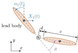
Figure 3: Sketch of the validation case adapted from Toomey and Eldredge [49].

Two cases from Toomey and Eldredge [49] are considered: Case 1 ($\sigma=0.628$) and Case 4 ($\sigma=3.770$). Fig. 4 depicts the kinematics of the lead body for both cases. The rest of parameters that fully define the problem are the rotation Reynolds number, $\mathit{Re}_{r}=\dot{\alpha}_{M}c^{2}/\nu=100$ (where $\dot{\alpha}_{\textit{M}}$ is the maximum angular velocity); the body-to-fluid density ratio, $\rho_{s}/\rho=5$; the dimensionless spring stiffness, $K^{*}=K/(\rho f^{2}c^{4})=456$; and the damping coefficient, $R^{*}=R/(\rho fc^{4})=3.95$.

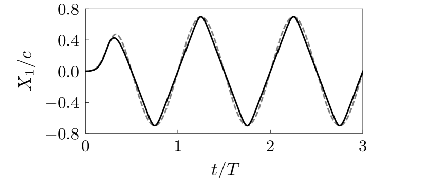
(a)

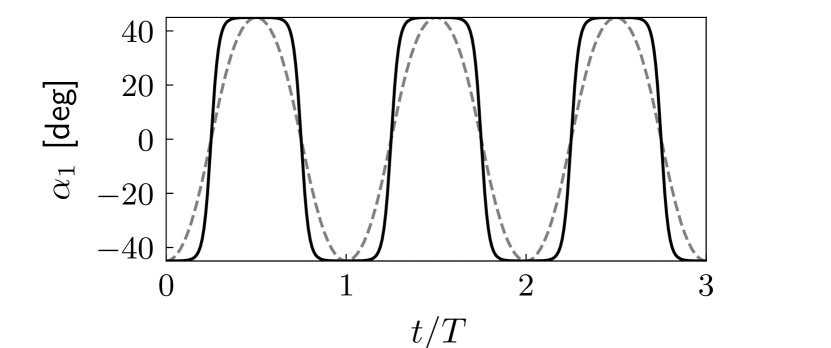
(b)

Figure 4: (a) Horizontal position and (b) pitch angle of the lead body as a function of time. ( ) Case 1; ( ) Case 4.

The results obtained with the present algorithm are compared with the results reported by Toomey and Eldredge [49] using a viscous vortex particle method, and with the results reported by Wang and Eldredge [29] using the IB-projection method. Note that both cases use strongly coupled body dynamics, while in the present algorithm the body dynamics are weakly coupled with the fluid solver.

In the present simulations, the computational domain is a square of side $32c$ (like in Wang and Eldredge [29]) with periodic boundary conditions. At $t=0$, the centre of mass of the lead body is located at $8c$ from the top wall and centred in the horizontal direction. The fluid domain is discretized with a uniform mesh of grid spacing $\Delta x=\Delta y=c/64$. This is a slightly coarser resolution than the one used in previous studies [49, 29] ($\Delta x\approx c/100$). The time step is set to $\Delta t=5\cdot 10^{-4}T$, leading to a Courant-Friedrichs-Lewy condition number, $\mathit{CFL}=\frac{U_{\textit{max}}\Delta t}{\Delta x}\leq 0.4$ (where $U_{\textit{max}}$ is the instantaneous maximum flow velocity in the fluid domain). Finally, the bodies are discretized using a Lagrangian mesh with evenly spaced points with distance $\Delta x$.

(a) Case 1

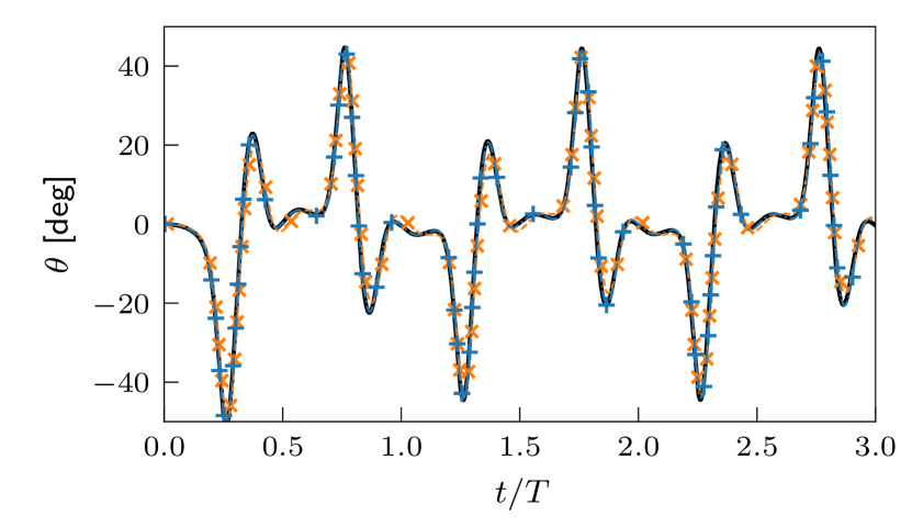
(b) Case 4

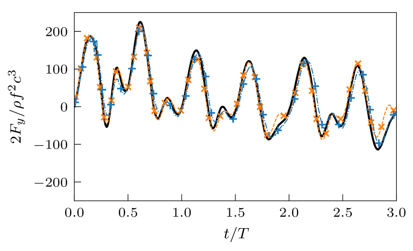
(c) Case 1

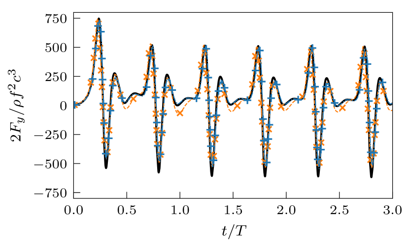
(d) Case 4

Figure 5: (a-b) Deflection angle of the follower body, and (c-d) total vertical force acting upon the multi-body system as a function of time. Note the difference in scale between cases 1 and 4. ( ) present results, ( ) Toomey and Eldredge [49], and ( ) Wang and Eldredge [29].

Fig. 5 depicts the comparison of the deflection angle, $\theta$, and the vertical force, $F_{y}$, between the current results and the existing literature. A good agreement of the evolution of the deflection angle, and the non-dimensional vertical force is observed for both cases despite the different numerical approaches and computational details.

3.2 Self-propelling flexible plate

The second validation case is taken from Arora et al. [26] and consists of a 2D self-propelling flexible plate. The plate is modelled using a lumped-torsional flexibility model as shown in Fig. 6(a). In particular, the plate of chord $C$ and thickness $e/C=0.02$ is divided into five rectangular rigid bodies, of uniform density, $\rho_{s}$, separated by a distance $2d=e$, joint by torsional springs of torsional stiffness, $K$. The plate is free to move in the horizontal direction, whereas the vertical position of the leading edge is prescribed as:

$$Y(t)=A\cos(2\pi ft)$$ (12)

The relative deflection angle of body $i$ with respect its predecessor, $i-1$, is defined as $\theta_{i}$ (see Fig. 6(a)). Consequently, the generalized vectors of the multi-body system are $\mathbf{q}_{p}=Y$ and $\mathbf{q}_{u}=[X,\,\theta_{1},...,\,\theta_{5}]$, where $X$ is the horizontal coordinate of the leading edge of the plate.

The parameters that govern the present problem are the non-dimensional amplitude, $A/C=0.6$; the Reynolds number, $\mathit{Re}=AfC/\nu=100$; the body-to-fluid density ratio, $\rho_{s}/\rho=10$; and the non-dimensional torsional stiffness, $K^{*}=K/\rho f^{2}C^{4}=52.242$. The chosen parameters correspond to the case $\psi={A\rho}/(e\rho_{s})=3$, $\omega^{*}=\omega_{n}/(2\pi f)=3.5$ (where $\omega_{n}$ is the first natural frequency of the multi-body system), shown in Arora et al. [26, Fig. 15 and 16].

(a)

(b)

Figure 6: (a) Lumped-torsional flexibility model of the flexible plate based on Arora et al. [26] consisting of 5 rectangular rigid bodies joined by torsional springs. (b) Extension of the model of Arora et al. [26] to three-dimensions by considering rectangular plates of width $b$.

The simulations are performed in a rectangular domain of size $20C\times 12C$ uniformly discretized with a grid size $\Delta x=\Delta y=0.004C$. Note that, due to the plunging motion of the plate’s leading edge (LE), it moves horizontally at an instantaneous speed $\dot{X}(t)$. Therefore, within each cycle the plate travels an horizontal distance $U_{p}T$, where $U_{p}=f\int_{T-1}^{T}\dot{X}\mathrm{d}t$ is the mean propulsive speed. In order to prevent the plate from leaving the computational domain, the plate is immersed in a uniform stream flow of intensity $U_{\infty}$ such that $U_{\infty}\approx U_{p}$ and the mean horizontal displacement of the plate with respect to the computational domain is as small as possible. Consequently, Dirichlet boundary conditions are imposed at the inflow and lateral walls on the horizontal ($u=U_{\infty}$) and vertical ($v=0$) fluid velocities. The value of $U_{\infty}$ equals the estimated mean propulsive velocity extracted from [26, Fig. 14]). An advective boundary condition is imposed at the outflow boundary. The bodies are discretized using a Lagrangian grid with equidistant points separated $\Delta x=0.004C$ and the time step is $\Delta t=5\cdot 10^{-5}T$ (where $T=f^{-1}$). On the other hand, simulations in Arora et al. [26] are performed using a Lattice-Boltzmann method with a larger computational domain ($50C\times 20C$) and a similar spatial resolution ($\Delta x=0.005C$).

Figure 7: Comparison of the (a) tip deflection angle, (b) horizontal force and (c) vertical force: ( ) present results, and ( ) Arora et al. [26]. In Fig. 7, ( ) corresponds to the $Y$-position of the leading edge (without scale).

Fig. 7a depicts the time evolution during two cycles of the tip deflection angle (defined as the angle between the horizontal and the line that joins the leading edge and the trailing edge). Fig. 7b-c shows the time evolution of the horizontal and vertical forces exerted on the plate normalized by $\frac{1}{2}\rho V^{2}C$, where $V=2\pi fA$ is the maximum vertical velocity of the leading edge. It should be pointed out that results from Arora et al. [26] correspond to cycles $48-49$, whereas the present results are for cycles $12-13$, since no changes were observed with respect to previous cycles. Nevertheless, a good agreement is observed between the present simulations and those from Arora et al. [26], with relative differences in the peak-to-peak amplitudes of the forces of less than $3\%$, and an absolute difference of the maximum tip-deflection angle lower than $0.19^{\circ}$.

3.3 Three-dimensional flapping flag in a free stream

The third case considered is the 3D flow around a flag, flapping freely in a uniform stream. This case has been studied by several authors [21, 50] using finite-element structural solvers. The objective of presenting this comparison is not to provide a direct validation of the multi-body algorithm (already proven in the previous subsections), but to exemplify the capabilities of a multi-body approximation to simulate the dynamics of flexible bodies.

The problem setup corresponds to the one reported by Lee and Choi [50]. It consists of a flexible, square flag of side length $C$ and thickness $e/C=0.01$, immersed in a uniform free-stream of velocity $U_{\infty}$. The flag-to-fluid density ratio is $\rho_{s}/\rho=100$, the non-dimensional elastic modulus of the flag is $E/\rho U_{\infty}^{2}=1008$, and $Re=U_{\infty}C/\nu=200$. The computational domain is a rectangular prism of size $8C\times 8C\times 2C$ in the streamwise ($x$), vertical ($y$) and spanwise directions ($z$), respectively. Dirichlet boundary conditions ($u_{x}=U_{\infty}$, $u_{y}=u_{z}=0$) are imposed at the top, bottom and inflow boundaries; periodic boundary conditions are imposed at the lateral boundaries; and an advective boundary condition is imposed at the outflow boundary. The leading edge of the flag is fixed and parallel to the $z$-axis, with its centre located at a distance $C$ downstream of the inflow boundary and centered in the $y$ and $z$ directions. A grid with uniform spacing $\Delta x=\Delta y=\Delta z=C/64$ is used to discretize a refined region which contains the flag, whereas a constant stretching factor of $1.5\%$ is applied to the grid in the streamwise and vertical directions outside the refined region. The time step is $\Delta t=0.002C/U_{\infty}$ ensuring $\textit{CFL}<0.28$.

The structural model of the flag only considers flexibility along the chordwise direction. It is an extension of the lumped-torsional model of Arora et al. [26] to three dimensions, as depicted in Fig. 6(b). Since $e\ll C$, the flag is assumed to be an infinitely thin surface, as in Tian et al. [21]. Thus, the rigid bodies in Fig. 6(b) become rectangular surfaces, discretized with a Cartesian distribution of Lagrangian points with a uniform spacing $\Delta x$. The total number of bodies conforming the flag is set to 25, with $d/C=0$. The torsional stiffness of the joints, $K$, is computed to match the natural frequency of the flag, yielding $K/\rho U_{\infty}^{2}C^{2}=2.129\cdot 10^{-3}$.

The self-sustained flapping motion of the flag is triggered by the initial condition, as in Lee and Choi [50]. Hence, at the beginning of the simulation the flag is flat, with an angle of attack $\alpha=0.1\pi$ rad with respect to the free-stream. As a consequence of this initial asymmetry with respect to the midplane, the flag starts a self-sustained flapping motion about its leading edge with a constant frequency. A total of number of 5 flapping cycles have been simulated with the multi-body algorithm, as in Lee and Choi [50].

Figure 8 displays the temporal evolution of the vertical and horizontal force coefficients, and the vertical displacement of the tip at midspan. The plot shows the last two cycles of the simulations. The results from Tian et al. [21] and Lee and Choi [50] are also shown for comparison. Note that, Tian et al. [21] and Lee and Choi [50] employ finite-element methods to model the flag, thus accounting for spanwise flexibility and twisting of the flag. However, for the case considered, the deformations along the span are small (see Fig. 14b of Lee and Choi [50]). Hence, even if the present multi-body model of the flag does not allow for spanwise flexibility, Fig. 8 shows that both the forces and the vertical displacement at the tip computed with the proposed algorithm are in good agreement with the previous references, in particular with those reported by Lee and Choi [50]. Discrepancies with the results provided by Tian et al. [21] might be due to the differences in the computational setup. Note that the time in Fig. 8 is normalized with the flapping period ($T$), which is a result of the simulation. Table 1 shows the Strouhal number ($St=fC/U_{\infty}$, where $f=1/T$ is the flapping frequency) for the present case and those from Tian et al. [21] and[50]. The differences in the $St$ of multi-body and finite-element models of the flag are smaller than $2\%$, consistent with the agreement shown in the amplitude of force coefficient and tip displacements in Fig.  8.

	$St$
Tian et al. [21]	$0.263$
Lee and Choi [50]	$0.265$
present results	$0.261$

Table 1: Comparison of the Strouhal number ($St$).

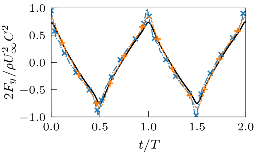
(a)

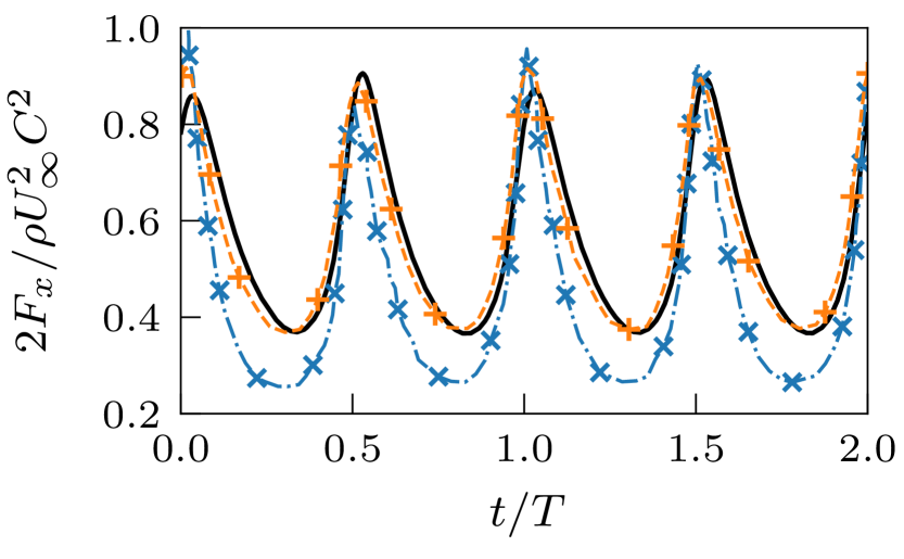
(b)

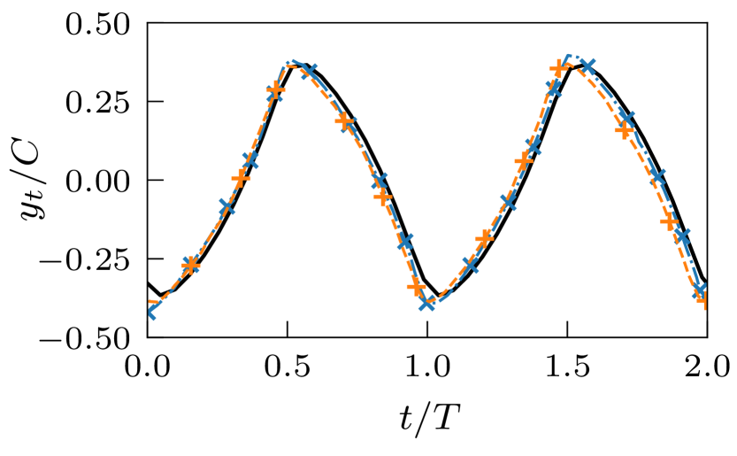
(c)

Figure 8: Comparison of the (a) Vertical force, (b) horizontal force and (c) vertical position of the tip at midspan. ( ) present results, ( ) Tian et al. [21], and ( ) Lee and Choi [50].

4 Results

In the next sections, two examples of the capabilities of the proposed methodology are presented. In §4.1 the study from Arora et al. [26] presented in §3.2 for validation is extended to a 3D configuration following the approach in §3.3. In §4.2 the proposed algorithm is employed to model a deformable filament attached to a sphere, as an idealized model of the spider ballooning problem.

4.1 Self propelling finite aspect ratio plate

We now extend the study of Arora et al. [26] by considering a flexible plate of finite span, $b=0.5C$, undergoing the same plunging motion given by eq. (12). The flexible plate with finite aspect ratio ($\AR=0.5$) is modelled using the lumped-torsional model of Arora et al. [26] (see Fig. 6(a)) extended to three dimensions, as depicted in Fig. 6(b).

In order to reduce the computational cost of the 3D configuration, a lower $Re$ than in § 3.2 is considered, allowing for a coarser spatial grid. Hence, both 2D and 3D flexible plates are simulated, to compare both configurations under the same conditions. The Reynolds number and the plunging amplitude in eq. (12) are set to $Re=20$ and $A/C=0.6$, respectively. On the other hand, the plunging frequency is selected as that of maximum propulsive speed for the 2D plate, namely $\omega^{*}=\omega_{n}/(2\pi f)\approx 5$ [26]. This leads to a torsional stiffness parameter $K^{*}=106.617$ for the 2D plate and a torsional stiffness parameter $K^{*}_{\textit{3D}}=K_{\textit{3D}}/(\rho f^{2}C^{5})=K^{*}\AR=53.309$ for the torsional springs of the 3D plate.

4.1.1 Computational set-up

Since the Reynolds number of these cases is five times smaller than that of the validation case discussed in § 3.2, a grid refinement study is performed for the 2D configuration to select the grid spacing, $\Delta x$, and the size of the computational domain.

Figure 9(a) displays the tip deflection angle during a cycle for 3 different values of $\Delta x=\Delta y$ in a computational domain of size $16C\times 8C$. As it can be appreciated, the trend of the tip angle is well captured even for the lowest grid resolution, $\Delta x=0.02C$. In particular, the relative error in the maximum tip angle is of $2\%$ and $0.5\%$ for $\Delta x=0.02C$ and $0.0125C$, respectively. Likewise, the effect of the external boundaries is evaluated by considering two sizes of the computational domain, $16C\times 8C$ and $40C\times 16C$, both discretized with a uniform grid spacing $\Delta x=\Delta y=0.02C$. The evolution of the tip angle during a cycle is displayed in Fig. 9(b) for both computational domains. The variation of the maximum tip angle with the fluid domain is less than $1\%$, implying that the location of the far field boundaries is not affecting the computed solution.

In sight of the previous results, the computational domain is chosen to be $16C\times 8C$ for the 2D simulation and $16C\times 8C\times 8C$ for the 3D simulation. The computational domain of the 2D simulations is discretized with a uniform grid of resolution $\Delta x=\Delta y=0.0125C$. For the 3D simulation, a uniform grid of resolution $\Delta x=\Delta y=\Delta z=0.02C$ is used to discretize a refined region which contains the plate, whereas a constant stretching factor of $1\%$ is applied to the grid in all directions outside the refined region. The size of the refined region is $4C\times 2C\times 2C$, being centred along the $y$ and $z$ directions and starting at $3C$ from the inflow boundary along the streamwise direction.

The boundary conditions of the 2D case are the same used for the validation case reported in section 3.2. For the 3D simulation, free-slip boundary conditions are imposed at all lateral boundaries, uniform streamwise flow of intensity $U_{\infty}$ at the inflow boundary, and an advective boundary condition at the outflow boundary. Note that, while $U_{p}$ is known from Arora et al. [26] for the 2D case and we can set $U_{\infty}=U_{p}$; it is not known a priori for its 3D counterpart. In order to estimate $U_{p}$, we first performed simulations fixing the horizontal position of the flapper, varying $U_{\infty}$ until the mean horizontal force over a cycle was approximately zero. Then, the simulation is restarted with this value of $U_{\infty}$, allowing the horizontal displacement of the flapper. Hence, the propulsive speed can be computed as:

$$U_{p}=U_{\infty}-\langle\dot{X}\rangle=U_{\infty}-\frac{1}{T}\int_{T-1}^{T}\dot{X}\mathrm{d}t,$$ (13)

where $\dot{X}$ is the instantaneous velocity of the leading edge of the plate with respect to the computational domain.

In terms of the IBM, all the surfaces are discretized into evenly distributed points separated by a distance $\Delta x$. The simulations are run until the forces on the plate are periodic and the value of $U_{p}$, computed with eq. (13), does not vary with respect to the previous cycle.

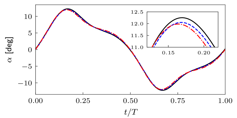
(a)

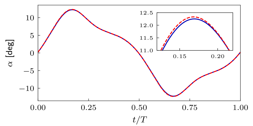
(b)

Figure 9: (a) Grid sensitivity analysis on the tip deflection angle, $\alpha$: ( ) $\Delta x=0.02C$, ( ) $\Delta x=0.0125C$, and ( ) $\Delta x=0.00625C$. (b) Effect of the fluid domain on $\alpha$: ( ) $16C\times 8C$, and ( ) $40\times 16C$.

4.1.2 Discussion of the results

One of the most noticeable differences between both cases is the change of the mean propulsive speed, $U_{p}$.

Table 2 shows that $U^{*}_{p}=U_{p}/V$ is three times lower for the $\AR=0.5$ flapper than for the 2D configuration. This result is consistent with the reduction in propulsion speed when $b/C$ decreases reported by Yeh and Alexeev [51] for plunging flexible plates at smaller plunging amplitude $A/C=0.1$ and at slightly higher $\mathit{Re}$ than the present one. Remarkably, Fig. 10 shows that the maximum tip deflection angle is similar in the 2D and 3D flappers, even if the phase-shift between the vertical position of the leading edge and the tip deflection angle is different: for the 2D case this phase-shift is close to $\pi/2$ ($\alpha\approx 0$ when $Y$ is maximum), but it is smaller for the 3D case.

	$U^{*}_{p}$	$\langle P^{*}_{i}\rangle$	$\varepsilon$
2D	$1.50$	$2.52$	$0.60$
3D	$0.48$	$1.44$	$0.33$

Table 2: Non-dimensionalized values of the propulsive speed, $U_{p}^{*}$, average input power, $\langle P_{i}^{*}\rangle$, and effectiveness, $\varepsilon$, for both cases.

The aerodynamic forces also change significantly from the 2D to the 3D scenario. This is appreciated in Fig. 10 and 10, which depict the aerodynamic forces normalized with the maximum vertical velocity and the reference surface, $S$. This reference surface is $C$ for the 2D case (since $F_{x}$ are forces per unit span) and $bC$ for the 3D case. In both cases, the tip deflection angle and the vertical force are in phase, suggesting that both, tip deflection and lift force, are direct consequences of the pressure difference between the upper and lower pressure acting upon the plate. A similar rationale holds for the horizontal force (Fig. 10); in both cases the peak thrust (negative $F_{x}$) occurs at the maximum tip deflection, meanwhile the drag (positive $F_{x}$) is maximum for $\alpha\approx 0$. Nonetheless, it can be observed that the drag and thrust peak have a similar amplitude for the 2D case, whereas the thrust peak for the 3D case is less pronounced. The smaller amplitude of $F_{x}$ in the 3D case is directly linked to a more steady instantaneous horizontal velocity (not shown).

Figure 10: Comparison of the (a) tip deflection angle, (b) horizontal force and (c) vertical force: ( ), 2D configuration and ( ) $\AR=0.5$ plate. In the normalization of the forces, $S=C$ for the 2D case and $S=bC$ for the 3D cases. In Fig. 10, ( ) corresponds to the position of the leading edge (without scale).

Figure 11 displays the vortical structures around the 3D flapper at the beginning of the downstroke (Fig. 11) and roughly at mid-downstroke (Fig. 11). The observed structures are qualitatively similar to those reported in the literature of similar flexible flappers but at post-resonance plunging frequencies [52, 51]. In particular, a leading edge vortex (LEV) and a pair of side tip vortices (STV) are developed at each stroke of the flapper. These vortices are shed at the end of each stroke and become a vortex ring which is convected downstream.

Figure 11: Visualization of the flow structures around the $\AR=0.5$ flapper at two time instants. Vortical structures are displayed as iso-contours of the $Q$ criterion [53]: light grey structures correspond to $Q=0.004V^{2}/C^{2}$ and red structures to $Q=7V^{2}/C^{2}$.

In order to compare the flow structure in both configurations, Fig. 12 depicts the spanwise vorticity $\omega_{z}$ and the pressure for the 2D case and for the mid-span ($z=0$) plane of the 3D case. It can be appreciated that the flow structure is clearly different in 2D and 3D, particularly in the wake of the flappers. Instead of the train of vortex dipoles observed in the 3D case (which correspond to the intersection of the vortex rings at $z=0$), the 2D wake consists of pairs of vortices with the same vorticity sign: an LEV_d formed during the downstroke and a TEV_u formed during the previous upstroke. The higher $U_{p}$ can be appreciated as a larger separation between vortices shed during each stroke in the 2D scenario, as compared to the 3D wake. Note also that in the 2D case, the LEV developed during upstroke (LEV_u) is shed at mid-downstroke, right before the shedding of the TEV that develops during the downstroke (TEV_d), as depicted in Fig. 12.

It is important to note that the LEV developed by the 2D plate is more intense, with a lower associated pressure, than to its 3D counterpart (see Fig. 12). Indeed, the lower pressure region associated to the 2D LEV could explain the smaller wing tip deflection at the beginning of a stroke: Fig. 12 reveals that at $t/T=0$, the 2D LEV_u is close to the trailing edge, making the plate to remain nearly horizontal. On the contrary, the LEV_u of the 3D flapper is still very close to the leading edge at the begining of the downstroke ($t=0$), resulting into a weaker suction on the lower surface of the flapper and correspondingly to a higher tip deflection.

Figure 12: Spanwise vorticity, $\omega_{z}$, and pressure contours for the 2D case and at mid-span of the 3D case at (a) beginning of the downstroke ($t/T=0$) and (b) mid-downstroke ($t/T=0.24$).

Finally, it is interesting to analyse the variation in the performance of the flappers. To that end, the effectiveness, or swimming economy of each plate is computed as [52, 51]:

$$\varepsilon=\frac{U_{p}^{*}}{\langle P_{i}^{*}\rangle},$$ (14)

where $\langle P_{i}^{*}\rangle$ is the average non-dimensional input power, namely, $P_{i}^{*}=2F_{y}\dot{Y}/(\rho V^{3}S)$, over the last cycle [26]. The values of $\langle P_{i}^{*}\rangle$ and $\varepsilon$ for both cases are gathered in Table 2. Although the required input power for the finite aspect ratio plate is lower than for its 2D counterpart, the reduction is not large enough to compensate for the lower propulsive speed. As a consequence, the swimming economy of the finite plate is significantly smaller than that of the 2D plate. Previous studies have linked the detriment of the swimming performance with decreasing $\AR$ with the STV [54, 51]. The absence of STV in the 2D case ($\AR\to\infty$), together with its greater performance, are in agreement with this hypothesis.

4.2 Spider ballooning

The second example of application of the methodology proposed here is inspired by the ability of some spiders to disperse aerially by releasing one or several silk filaments. These filaments act as drag lines when they encounter a wind current, allowing spiders to achieve long dispersal distances. This mechanism is usually known as spider ballooning [55, 56, 57]. Several studies addressing this phenomena can be found in the literature, either using experimental methods [58, 57, 59] or numerical methods [55, 60, 56], with the latter restricted to 2D configurations. These studies use actual samples or simplified models to characterize different parameters and performance metrics of spider ballooning (like the effective length of the filaments, or dispersal lengths and terminal descent velocities).

Motivated by this problem, we present here a fundamental study of the flow around a deformable filament of length $L$ attached to a sphere of diameter $D$. In particular, the objective of the study is to determine what is the effect of the filament on the flow around the sphere, as well as the fluid forces acting upon it. From the point of view of the filament, this problem can be classified as an extraneously induced excitation (EIE) fluid-induced vibration problem [61, 62].

Two simulations are performed: a fixed sphere immersed in a uniform flow (case S), and the same problem but with a deformable filament attached to the surface of the sphere (case F). The filament is modelled as $N$ rigid links connected among them by joints which do not restrain the rotation (see Fig. 13(a)). For the dynamical model, the links are modelled as cylindrical rods of constant density $\rho_{s}=6\rho$, length $l=L/N$ and diameter, $d=\Delta x$ (where $\Delta x$ is the grid size). For the fluid coupling, each link is discretized into a 1D array of $l/\Delta x$ points evenly distributed. Consequently, the fluid does not exert any torque along the longitudinal axis of the filament. This enables to define the position of a given link $i$ with respect to its predecessor by means of two angles, $\theta_{i}$ and $\varphi_{i}$ (see Fig. 13(b)), instead of 3, as should be required to define the orientation of a rigid body. Accordingly, the joint connecting a given link, $i$, with its predecessor, $i-1$, is a multi-DOF joint consisting of a revolute joint about the $y_{i}-$axis, followed by another revolute joint about the rotated $z_{i}-$axis, namely, $z_{i}^{\prime}$, as sketched in Fig. 13(b).

(a)

(b)

Figure 13: (a) Sketch of the multi-body system composed of a fixed sphere and filament consisting of $N=6$ links. The reference frame depicted corresponds to the inertial reference frame. (b) Schematic view of the parameters that define the joint between two linkages. The Cartesian frame $x_{i}y_{i}z_{i}$ is fixed to the link $i-1$.

The sphere is immersed in a uniform flow parallel to the $x$-axis (see Fig. 13(a)) of magnitude $U$. The point at which the filament is attached is $x=-D/2$, that is, at the downstream end of the sphere. For the present study, $L=5D$, $\mathit{Re}=DU/\nu=300$, and $N=24$. This Reynolds number corresponds to a flow regime for the case of the isolated sphere in which vortex shedding starts to occur [63], and it has been selected to explore the interference between the filament and the vortex shedding process.

4.2.1 Computational set-up

For both simulations, the computational domain is a rectangular prism of dimensions $14D\times 8D\times 8D$ in the streamwise and lateral directions, respectively. A refined region of size $7D\times 2D\times 2D$ is defined, with a uniform resolution $\Delta x=\Delta y=\Delta z=D/48$. This region is located $3D$ downstream of the inflow, centered within the lateral directions of the computational domain. Outside of this region, a stretching factor of $1\%$ is applied in all directions. A uniform free stream of magnitude $U$ is imposed at the inflow boundary, free-slip boundary conditions are imposed at the lateral boundaries and an advective boundary conditions is implemented at the outflow boundary.

For the IBM, the sphere is discretized into $N_{s}$ evenly distributed points, such that $N_{s}\approx\pi D^{2}/\Delta x^{2}$, similarly to Uhlmann [12]. On the other hand, each segment of the filament is discretized by equally spaced points, separated a distance $\Delta x$, without gaps between adjacent segments.

The time step is fixed to $\Delta t=0.0025U/D$, ensuring $\textit{CFL}<0.2$. Finally, the simulation of the isolated sphere (case S) is started from scratch, whereas the sphere with the attached filament (case F) is started from a flow field of case S when vortex shedding was present.

4.2.2 Discussion of the results

At the selected Reynolds number, the flow over the sphere exhibits periodic shedding of vortices after an initial transient. Fig. 14 displays an snapshot of the wake of the sphere after the onset of vortex shedding. This leads to oscillatory hydrodynamic forces over the sphere, as observed from Fig. 15, which depicts the non-dimensional streamwise (i.e., drag) force, $F_{x}^{*}=F_{x}/(\rho U^{3}\pi D^{2}/8)$. It can also be observed that the mean value of $F_{x}^{*}$ increases after the onset of vortex shedding. The oscillation frequency is found to be $0.135U/D$, in agreement with existing literature at the same Reynolds number [64, 65]. Furthermore, the non-axisymmetric wake leads to the appearance of a transversal force contained in the plane of symmetry of the wake. Note that the location of this plane of symmetry with respect to the inertial axis arises naturally, only forced by numerical biases [65]. In the present case, the angle between the $(x,y)-$plane and the symmetry plane is approximately $67.7^{\circ}$. This angle, is computed by a least square regression of the transversal forces, as shown in in Fig. 15. Figure 15 depicts the transverse force when expressed in parallel ($F_{\parallel}$) and perpendicular ($F_{\bot}$) components with respect to the symmetry plane of the wake. The plot shows oscillations of $F^{*}_{\parallel}$, with the same frequency of oscillation as $F^{*}_{x}$, and a net non-zero $F^{*}_{\parallel}$ when averaged over several periods.

Figure 14: Instantaneous visualization of the flow structures around the isolated sphere at $\mathit{Re}=300$. Vortical structures correspond to iso-contours of the $Q$-criterion, $Q=0.2U^{2}/D^{2}$.

Figure 15: (a) Temporal evolution of the non-dimensional streamwise force. ( ) case S; ( ) case F (force over the sphere); ( ) case F (force over the sphere and the filament). (b) ( ) Non-dimensional transverse force on the sphere for case S for $t>90D/U$ (after onset of vortex shedding); and its ( ) least square regression. (c) Temporal evolution of the non-dimensional transverse forces expressed into its parallel and normal components. Color legend is as 15, line styles stands for ( ) $F_{\parallel}^{*}$, and ( ) $F_{\bot}^{*}$.

When the deformable filament is attached to the posterior part of the sphere, the flow topology is greatly modified. If the simulation is started from a flow field with vortical structures (Fig. 16(a)) the filament starts oscillating, and after 2-3 shedding cycles, vortex shedding is suppressed, and a stable flow around the sphere-filament is developed (Fig. 16(b)). If the simulations are started from scratch, no vortex shedding occurs. The topology of the flow in this new regime is characterized by the development of an axisymmetric recirculation region attached to the sphere, similarly to the case of the isolated sphere at $\mathit{Re}<210$ [65]. This can be clearly appreciated in Fig. 17, which depicts the instantaneous streamlines past the sphere and the filament. Note that a shear layer is developed along the filament, which changes direction in the recirculation bubble.

(a)

(b)

Figure 16: Instantaneous visualization of the flow structures around the sphere with the deformable filament at (a) initial time instants, and (b) after reaching and stable state. Vortical structures correspond to iso-contours of the $Q$-criterion, $Q=0.2U^{2}/D^{2}$, as in Fig. 14.

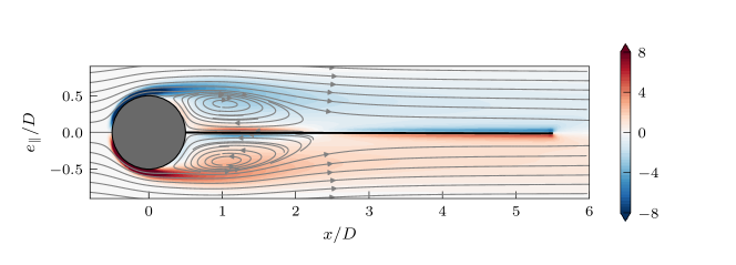
Figure 17: Instantaneous streamlines past the sphere and the filament in the $(x,e_{\parallel})$-plane, together with the vorticity perpendicular to the plane.

The vortex shedding inhibition has a noticeable effect on the forces acting over the sphere. Firstly, the mean drag force acting over the sphere is reduced and the oscillations are hindered, as shown in Fig. 15, leading to a steady value of the drag force over the sphere. However, the total drag force (i.e., sphere + filament) increases, due to the skin friction of the filament, which acts as a drag line. Secondly, the amplitude of the oscillations of the transverse force decreases with respect to the case of the isolated sphere, as shown in Fig. 15. The frequency of oscillation of the transverse forces (which was previously linked to the shedding frequency of vortices over the sphere) is also reduced, from $0.135U/D$ without the filament to $0.120U/D$ with the filament.

In addition, the mean value of the transverse force over an oscillation cycle has a zero mean value (Fig. 15), which suggest that the flow becomes symmetric, in a time-average sense, across the $(x,e_{\parallel})-$plane (where $e_{\parallel}$ is the direction perpendicular to $x-$axis and contained in the wake’s symmetry plane).

Regarding the dynamics of the filament, Fig. 18 depicts its deformation pattern during the last two oscillation cycles of the transverse force. It can be observed that the filament is not steady but it oscillates with a low amplitude. It is interesting to note that these oscillations are contained in a plane, which correspond to the symmetry plane of the wake of the isolated sphere.

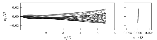
Figure 18: Oscillation pattern of the filament during the last two oscillation cycles of the transverse forces. Line color indicates the time instant (from grey to black). Note the difference in the scale of the axes.

5 Conclusions

A methodology to solve fluid-structure interaction problems with multi-body systems has been presented. The proposed methodology follows a partitioned approach. The flow is solved using a conventional fractional-step method, while the presence of the bodies of the MBS in the fluid is imposed by means of the immersed boundary method proposed by Uhlmann [12]. On the other hand, the dynamic equations of the rigid bodies are computed in terms of the reduced coordinates of the MBS by the CRBA and RNEA recursive algorithms proposed by Felis [33]. The coupling between flow equations and the MBS equations is weak, extending the approach of Uhlmann [12] for single rigid bodies to MBSs.

Since the flow solver has been already validated elsewhere, the validation focuses on the multi-body dynamics and the coupling. Three cases from the literature have been selected to that end. The first validation case corresponds to a system of two bodies joined by a torsional spring. Very good agreement is obtained when comparing to a vortex particle method [49] and to a vorticity-based IBM with strong coupling [29]. The second case corresponds to a flexible, self-propelled plate modelled as several rigid bodies connected by torsional springs [26]. Again, the agreement between the results of the present methodology and the Lattice-Boltzmann simulation of the reference is very good. In the third case, the proposed methodology is used to simulate the dynamics of a three-dimensional flexible flag and compare against results using a finite-element formulation of the structure. A remarkable good agreement is found, in terms of the kinematics and dynamics, between the present methodology and the finite-element structural solvers.

Two additional bio-inspired examples are analized to illustrate the capabilities of the present methodology. The first example is a three-dimensional extension of the case presented by Arora et al. [26]. It is observed that 3D effects are detrimental in terms of propulsive speed and efficiency, although the deflection of the plate is not significantly modified. The results are in accordance with those reported by Yeh and Alexeev [52] for flexible self-propelled plates. The second example is loosely inspired by the ballooning mechanism of several spiders to disperse aerially. The problem is modelled as a deformable filament attached to a fixed sphere and immersed in a free-stream. The flexibility of the filament is modelled as a chain of rigid links connected with multi-DoF joints. When compared to an isolated sphere at the same Reynolds number, it is shown that the vortex shedding is suppressed by the filament, which oscillates with very low amplitudes in the wake of the sphere. The reduction in the unsteadiness of the flow results in a decrease of the drag contribution from the sphere. However, a larger total drag is obtained, due to the extra friction introduced by the filament.

In summary, it has been shown that the proposed methodology allows the definition and analysis of a multitude of diverse configurations of MBS, thanks to the use of generalised recursive algorithms. Moreover, the coupling between the flow equations and the MBS equations is very simple, yet robust enough to provide very good agreement with existing results from the literature. Nonetheless, the weak coupling imposes a lower limit on the density ratios of the bodies which can be simulated with the present methodology. Although, recent works have proven to successfully tackle arbitrary density ratios for single rigid bodies using a non-iterative version of the weak coupling approach presented here [48], the technical details are not trivial for arbitrary geometries so that this extension of the methodology is left for future work.

Appendix A Joint modelling

A joint that connect two bodies can also be regarded as the constraint of the relative motion between two Cartesian reference frames, attached to each body [24]. Figure 19(a) illustrates this concept: body $\Gamma_{i}$ has an attached reference frame, $\Sigma_{i}$, and is linked to its predecessor body, $\Gamma_{k}$, which has its own attached reference frame, $\Sigma_{k}$. Therefore, a joint can be defined by the rotation matrix, $\mathsf{E}_{k,i}$, from $\Sigma_{i}$ to $\Sigma_{k}$; and the vector $\mathbf{s}_{i}$, which links the origin of both Cartesian frames and is implicitly expressed in $\Sigma_{k}$. Note that $\mathsf{E}_{k,i}$ and $\mathbf{s}_{i}$ only depend on the degrees of freedom allowed by the joint, but their definition depend on the kind of joint.

Single DoF joints of two types are considered: prismatic (i.e., translation) joints along any axis of $\Sigma_{k}$; and revolute (i.e. rotation) joints about any axis of $\Sigma_{k}$. For a prismatic joint which allows translation along the $x$-axis of $\Sigma_{k}$, $\mathsf{E}_{k,i}$ is the identity matrix of size $3$; and $\mathbf{s}_{i}(q_{i})=q_{i}\mathbf{e}_{x}$, where $\mathbf{e}_{x}$ is the unitary vector parallel to $x$-axis, and $q_{i}$ is the joint’s degree of freedom and corresponds to the magnitude of the translation. Then, the relative velocity of body $\Gamma_{i}$ with respect to $\Sigma_{k}$ is:

$$\bm{\omega}_{i}^{\prime} =\mathbf{0}, \mathbf{v}_{i}^{\prime} =\dot{\mathbf{s}}_{i}=\dot{q}_{i}\mathbf{e}_{x}.$$

On the other hand, for a joint which allows the rotation about the $x$-axis, $\mathsf{E}_{k,i}(q_{i})$ is a matrix belonging to the 3D rotation group, $SO(3)$, namely

$$\mathsf{E}_{k,i}(q_{i})=\begin{bmatrix}1&0&0\\ 0&\cos{q_{i}}&-\sin{q_{i}}\\ 0&\sin{q_{i}}&\cos{q_{i}}\\ \end{bmatrix};$$

and $\mathbf{s}_{i}$ is a constant vector. Note that, in this case $q_{i}$ stands for the rotation angle. In this case, the relative velocity of body $\Gamma_{i}$ with respect to $\Sigma_{k}$ takes the form:

$$\bm{\omega}_{i}^{\prime} =\dot{q}_{i}\mathbf{e}_{x}, \mathbf{v}_{i}^{\prime} =\bm{\omega}_{i}^{\prime}\times\mathbf{s}_{i}.$$

Similar definitions stand for translations and rotations about $y$ and $z$ axes.

In order to model joints which allow multiple degrees of freedom between two bodies, several virtual bodies can be linked sequentially using single DoF joints (prismatic or revolute), as illustrated in Fig. 19(b). For the dynamical model, these virtual bodies have no mass; and for the fluid coupling, they have no associated Lagrangian points (i.e., no volume). Under this approach, the connection between the two physical bodies is equivalent to a multi DoF joint. Hence, the present methodology allows a simple implementation of any kind of kinematic joint with a negligible increase of the computational cost.

(a)

(b)

Figure 19: (a) Sketch of body $\Gamma_{i}$ and its predecessor, $\Gamma_{k}$, illustrating the elements that define the joint between them. (b) Representation of a joint with $3$ DoF, simulated by means of 2 virtual bodies (represented as dashed circles) which have no mass and associated Lagrangian points.

Appendix B Mapping between generalized and physical coordinates

B.1 From generalized coordinates to physical coordinates

Computation of $\mathbf{X}_{i,j}$ and $\mathbf{U}_{\partial\Gamma_{i}}$, according to eq. (10), requires the calculation of $\mathsf{E}_{i}$, $\mathbf{x}_{i}^{0}$, $\mathbf{v}_{i}^{0}$, and $\mathbf{\omega}_{i}^{0}$. These variables can be derived from the joint variables derived in A. To that end, we exploit the fact that, for a kinematic tree like the one considered in Fig. 1(a), we can define a unique predecessor for each body, $\Gamma_{i}$, which can be hence denoted as $\Gamma_{\lambda(i)}$. Likewise, a set $\mu(i)$ can be defined containing all the bodies which precede $\Gamma_{i}$. As an example, for body $\Gamma_{7}$ in Fig. 1(a), $\mu(7)=\{4,\,5,\,7\}$. Under these definitions, the rotation matrix of body $\Gamma_{i}$ is computed as:

$$\mathsf{E}_{i}=\prod_{j\in\mu(i)}\mathsf{E}_{\lambda(j),j}$$ (15)

Likewise,

$$\mathbf{x}_{i}^{0}=\sum_{j\in\mu(i)}\mathsf{E}_{\lambda(j)}\mathbf{s}_{j}(q_{j}),$$ (16)

whereas, $\mathbf{v}_{i}^{0}$ and $\bm{\omega}_{i}^{0}$ can be computed from eq. (16) by substituting $\mathbf{s}_{j}$ by $\mathbf{v}_{j}^{\prime}$ and $\bm{\omega}_{j}^{\prime}$, respectively.

B.2 From physical coordinates to generalized coordinates

In order to compute $\bm{\xi}_{h}$ to solve eq. (7), the hydrodynamic forces acting upon the bodies must be expressed in terms of generalized coordinates. Note that, with the present coupling, the component of the hydrodynamic forces that have to be mapped are $\mathcal{G}_{i}$ and $\mathcal{N}_{i}$ from eq. (11a) and eq. (11b), respectively. For the sake of efficiency, it is convenient to gather both forces and moments acting on body $\Gamma_{i}$ into a single vector:

$$\hat{\mathbf{f}}_{i}^{h}=\begin{bmatrix}\mathcal{N}_{i}\\ \mathcal{G}_{i}\end{bmatrix},$$ (17)

where it is implicitly assumed that both $\mathcal{N}_{i}$ and $\mathcal{G}_{i}$ are expressed in $\Sigma_{0}$ and moments are computed about the origin.

We also define the matrix transform of $\Gamma_{i}$ as:

$$\mathbf{X}^{*}_{i}=\begin{bmatrix}\mathsf{E}_{i}^{\top}&-\mathsf{E}_{i}^{\top}{\mathbf{x}_{i}^{0}\times}\\ \mathsf{0}&\mathsf{E}_{i}^{\top}\end{bmatrix},$$ (18)

where ${\mathbf{x}_{i}^{0}\times}$ is a skew-symmetric matrix belonging to the Lie algebra of the $SO(3)$ rotation group.

With the previous definitions, a simplified version of the RNEA can be implemented to compute the components of $\bm{\xi}_{h}$, namely:

for $i\leftarrow 1,N_{B}$ do

     $\hat{\mathbf{g}}_{i}=\mathbf{X}^{*}_{i}\hat{\mathbf{f}}_{i}^{h}$

end for

for $i\leftarrow N_{B},1$ do

     $\xi_{h,i}=\mathbf{S}_{i}^{\top}\hat{\mathbf{g}}_{i}$

     if $\lambda(i)\neq 0$ then

         $\hat{\mathbf{g}}_{\lambda(i)}=\hat{\mathbf{g}}_{\lambda(i)}+\mathbf{X}^{*}_{\lambda(i)}\hat{\mathbf{f}}_{i}^{h}$

     end if

end for

where $\lambda(i)$ is the index of the predecessor body of $\Gamma_{i}$. The previous algorithm simply transfers the forces acting upon a given body across its supporting tree (i.e., the set of bodies that connect it to base, $\Sigma_{0}$). Note that, $\mathbf{S}_{i}$ is the motion subspace of the joint. For prismatic and revolute joints, $\mathbf{S}_{i}$ is a unitary column vector of size $6\times 1$, whose only non-zero component is the axis along which rotation/translation is allowed. In particular, its first 3 components are associated to rotations about the $x$, $y$ or $z$ axes of the joints; meanwhile its 3 last components are associated with translations along the aforementioned axes.

References

- de Croon et al. [2009] G. de Croon, K. de Clercq, R. Ruijsink, B. Remes, C. de Wagter, Design, aerodynamics, and vision-based control of the DelFly, Int. J. Micro Air Veh. 1 (2009) 71–97. doi:10.1260/175682909789498288.
- Richter and Lipson [2011] C. Richter, H. Lipson, Untethered hovering flapping flight of a 3D-printed mechanical insect, Artif. Life 17 (2011) 73–86. doi:10.1162/artl\_a\_00020.
- Keennon et al. [2012] M. Keennon, K. Klingebiel, H. Won, Development of the nano hummingbird: A tailless flapping wing micro air vehicle, in: 50th AIAA Aerospace Sciences Meeting including the New Horizons Forum and Aerospace Exposition, 2012, pp. 1–12. doi:10.2514/6.2012-588.
- Triantafyllou and Triantafyllou [1995] M. S. Triantafyllou, G. S. Triantafyllou, An efficient swimming machine, Sci. Am. 272 (1995) 64–70.
- Hirata et al. [2000] K. Hirata, T. Takimoto, K. Tamura, Study on turning performance of a fish robot, in: Proc. 1st Int. Symp. Aqua Bio-Mechanisms, 2000, pp. 287–292.
- Yu et al. [2004] J. Yu, M. Tan, S. Wang, E. Chen, Development of a biomimetic robotic fish and its control algorithm, IEEE Transactions on Systems, Man, and Cybernetics, Part B (Cybernetics) 34 (2004) 1798–1810. doi:10.1109/TSMCB.2004.831151.
- Deng et al. [2013] H.-B. Deng, Y.-Q. Xu, D.-D. Chen, H. Dai, J. Wu, F.-B. Tian, On numerical modeling of animal swimming and flight, Comput. Mech. 52 (2013) 1221–1242. doi:10.1007/s00466-013-0875-2.
- Donea et al. [2017] J. Donea, A. Huerta, J.-P. Ponthot, A. Rodríguez-Ferran, Arbitrary Lagrangian–Eulerian Methods, in: Encyclopedia of Computational Mechanics Second Edition, Wiley Online Library, 2017, pp. 1–23. doi:10.1002/9781119176817.ecm2009.
- Tschisgale and Fröhlich [2020] S. Tschisgale, J. Fröhlich, An immersed boundary method for the fluid-structure interaction of slender flexible structures in viscous fluid, J. Comput. Phys. 423 (2020) 109801. doi:10.1016/j.jcp.2020.109801.
- Mittal and Iaccarino [2005] R. Mittal, G. Iaccarino, Immersed boundary methods, Annu. Rev. Fluid Mech. 37 (2005) 239–261. doi:10.1146/annurev.fluid.37.061903.175743.
- Griffith and Patankar [2020] B. E. Griffith, N. A. Patankar, Immersed methods for fluid–structure interaction, Annu. Rev. Fluid Mech. 52 (2020) 421–448. doi:10.1146/annurev-fluid-010719-060228.
- Uhlmann [2005] M. Uhlmann, An immersed boundary method with direct forcing for the simulation of particulate flows, J. Comput. Phys. 209 (2005) 448–476. doi:10.1016/j.jcp.2005.03.017.
- Pinelli et al. [2010] A. Pinelli, I. Z. Naqavi, U. Piomelli, J. Favier, Immersed-boundary methods for general finite-difference and finite-volume Navier–Stokes solvers, J. Comput. Phys. 229 (2010) 9073–9091. doi:10.1016/j.jcp.2010.08.021.
- Breugem [2012] W.-P. Breugem, A second-order accurate immersed boundary method for fully resolved simulations of particle-laden flows, J. Comput. Phys. 231 (2012) 4469–4498. doi:10.1016/j.jcp.2012.02.026.
- Kempe and Fröhlich [2012] T. Kempe, J. Fröhlich, An improved immersed boundary method with direct forcing for the simulation of particle laden flows, J. Comput. Phys. 231 (2012) 3663–3684. doi:10.1016/j.jcp.2012.01.021.
- Bhalla et al. [2013] A. P. S. Bhalla, R. Bale, B. E. Griffith, N. A. Patankar, A unified mathematical framework and an adaptive numerical method for fluid–structure interaction with rigid, deforming, and elastic bodies, J. Comput. Phys. 250 (2013) 446–476. doi:10.1016/j.jcp.2013.04.033.
- Wiens and Stockie [2015] J. K. Wiens, J. M. Stockie, An efficient parallel immersed boundary algorithm using a pseudo-compressible fluid solver, J. Comput. Phys. 281 (2015) 917–941. doi:10.1016/j.jcp.2014.10.058.
- de Tullio and Pascazio [2016] M. de Tullio, G. Pascazio, A moving-least-squares immersed boundary method for simulating the fluid–structure interaction of elastic bodies with arbitrary thickness, J. Comput. Phys. 325 (2016) 201–225. doi:10.1016/j.jcp.2016.08.020.
- Kim and Peskin [2009] Y. Kim, C. S. Peskin, 3-d parachute simulation by the immersed boundary method, Comput. Fluids 38 (2009) 1080–1090. doi:10.1016/j.compfluid.2008.11.002.
- Zhang et al. [2004] L. Zhang, A. Gerstenberger, X. Wang, W. K. Liu, Immersed finite element method, Comput. Methods Appl. Mech. Eng. 193 (2004) 2051–2067. doi:10.1016/j.cma.2003.12.044.
- Tian et al. [2014] F.-B. Tian, H. Dai, H. Luo, J. F. Doyle, B. Rousseau, Fluid–structure interaction involving large deformations: 3d simulations and applications to biological systems, J. Comput. Phys. 258 (2014) 451–469. doi:10.1016/j.jcp.2013.10.047.
- Liu [2009] H. Liu, Integrated modeling of insect flight: From morphology, kinematics to aerodynamics, J. Comput. Phys. 228 (2009) 439 – 459. doi:10.1016/j.jcp.2008.09.020.
- Suzuki et al. [2015] K. Suzuki, K. Minami, T. Inamuro, Lift and thrust generation by a butterfly-like flapping wing–body model: immersed boundary–lattice Boltzmann simulations, J. Fluid Mech. 767 (2015) 659 – 695. doi:10.1017/jfm.2015.57.
- Featherstone [2014] R. Featherstone, Rigid body dynamics algorithms, Springer, 2014.
- Zhang et al. [2013] S. Zhang, J. Yu, A. Zhang, F. Zhang, Spiraling motion of underwater gliders: Modeling, analysis, and experimental results, Ocean Eng. 60 (2013) 1–13. doi:10.1016/j.oceaneng.2012.12.023.
- Arora et al. [2018] N. Arora, C.-K. Kang, W. Shyy, A. Gupta, Analysis of passive flexion in propelling a plunging plate using a torsion spring model, J. Fluid Mech. 857 (2018) 562–604. doi:10.1017/jfm.2018.736.
- Suzuki et al. [2019] K. Suzuki, I. Okada, M. Yoshino, Effect of wing mass on the free flight of a butterfly-like model using immersed boundary–lattice Boltzmann simulations, J. Fluid Mech. 877 (2019) 614–647. doi:10.1017/jfm.2019.597.
- Yao and Yeo [2019] J. Yao, K. S. Yeo, Free hovering of hummingbird hawkmoth and effects of wing mass and wing elevation, Comput. Fluids 186 (2019) 99 – 127. doi:10.1016/j.compfluid.2019.04.007.
- Wang and Eldredge [2015] C. Wang, J. D. Eldredge, Strongly coupled dynamics of fluids and rigid-body systems with the immersed boundary projection method, J. Comput. Phys. 295 (2015) 87–113. doi:10.1016/j.jcp.2015.04.005.
- Li et al. [2018] R. Li, Q. Xiao, Y. Liu, J. Hu, L. Li, G. Li, H. Liu, K. Hu, L. Wen, A multi-body dynamics based numerical modelling tool for solving aquatic biomimetic problems, Bioinspir. Biomim. 13 (2018) 056001. doi:10.1088/1748-3190/aacd60.
- Bernier et al. [2019] C. Bernier, M. Gazzola, R. Ronsse, P. Chatelain, Simulations of propelling and energy harvesting articulated bodies via vortex particle-mesh methods, J. Comput. Phys. 392 (2019) 34 – 55. doi:10.1016/j.jcp.2019.04.036.
- Gazzola et al. [2011] M. Gazzola, P. Chatelain, M. v. R. Wim, P. Koumoutsakos, Simulations of single and multiple swimmers with non-divergence free deforming geometries, J. Comput. Phys. 230 (2011) 7093 – 7114. doi:10.1016/j.jcp.2011.04.025.
- Felis [2017] M. Felis, RBDL: an efficient rigid-body dynamics library using recursive algorithms, Auton. Robot. 41 (2017) 495–511. doi:10.1007/s10514-016-9574-0.
- Greenwood [2006] D. Greenwood, Advanced dynamics, Cambridge University Press, 2006.
- Boyer and Porez [2015] F. Boyer, M. Porez, Multibody system dynamics for bio-inspired locomotion: From geometric structures to computational aspects, Bioinspir. Biomim. 10 (2015) 1–21. doi:10.1088/1748-3190/10/2/025007.
- Rai and Moin [1991] M. Rai, P. Moin, Direct simulations of turbulent flow using finite-difference schemes, J. Comput. Phys. 96 (1991) 15 – 53. doi:10.1016/0021-9991(91)90264-L.
- Peskin [2002] C. Peskin, The immersed boundary method, Acta Numer. 11 (2002) 479–51. doi:10.1017/S0962492902000077.
- Roma et al. [1999] A. M. Roma, C. S. Peskin, M. J. Berger, An adaptive version of the immersed boundary method, J. Comput. Phys. 153 (1999) 509–534. doi:10.1006/jcph.1999.6293.
- Sotiropoulos and Yang [2014] F. Sotiropoulos, X. Yang, Immersed boundary methods for simulating fluid–structure interaction, Prog. Aerosp. Sci. 65 (2014) 1–21. doi:10.1016/j.paerosci.2013.09.003.
- Moriche et al. [2016] M. Moriche, O. Flores, M. García-Villalba, Three-dimensional instabilities in the wake of a flapping wing at low Reynolds number, Int. J. Heat Fluid Flow 62A (2016) 44–55. doi:10.1016/j.ijheatfluidflow.2016.06.015.
- Moriche et al. [2017] M. Moriche, O. Flores, M. García-Villalba, On the aerodynamic forces on heaving and pitching airfoils at low Reynolds number, J. Fluid Mech. 828 (2017) 395–423. doi:10.1017/jfm.2017.508.
- Gonzalo et al. [2018] A. Gonzalo, G. Arranz, M. Moriche, M. García-Villalba, O. Flores, From flapping to heaving: A numerical study of wings in forward flight, J. Fluids Struct. 83 (2018) 293–309. doi:10.1016/j.jfluidstructs.2018.09.006.
- Arranz et al. [2020] G. Arranz, O. Flores, M. García-Villalba, Three-dimensional effects on the aerodynamic performance of flapping wings in tandem configuration, J. Fluids Struct. 94 (2020) 102893. doi:10.1016/j.jfluidstructs.2020.102893.
- Moriche et al. [2021a] M. Moriche, A. Gonzalo, O. Flores, M. Garcia-Villalba, Three-dimensional effects on plunging airfoils at low Reynolds numbers, AIAA J. 59 (2021a) 65–74. doi:10.2514/1.J058569.
- Moriche et al. [2021b] M. Moriche, G. Sedky, A. R. Jones, O. Flores, M. Garcia-Villalba, Characterization of aerodynamic forces on wings in plunge maneuvers, AIAA J. 59 (2021b) 751–762. doi:10.2514/1.J059689.
- Arranz et al. [2018a] G. Arranz, M. Moriche, M. Uhlmann, O. Flores, M. García-Villalba, Kinematics and dynamics of the auto-rotation of a model winged seed, Bioinspir. Biomim. 13 (2018a) 036011. doi:10.1088/1748-3190/aab144.
- Arranz et al. [2018b] G. Arranz, A. Gonzalo, M. Uhlmann, O. Flores, M. García-Villalba, A numerical study of the flow around a model winged seed in auto-rotation, Flow Turbul. Combust. 101 (2018b) 477–497. doi:10.1007/s10494-018-9945-z.
- Tschisgale et al. [2017] S. Tschisgale, T. Kempe, J. Fröhlich, A non-iterative immersed boundary method for spherical particles of arbitrary density ratio, J. Comput. Phys. 339 (2017) 432 – 452. doi:10.1016/j.jcp.2017.03.026.
- Toomey and Eldredge [2008] J. Toomey, J. D. Eldredge, Numerical and experimental study of the fluid dynamics of a flapping wing with low order flexibility, Phys. Fluids 20 (2008) 073603. doi:10.1063/1.2956372.
- Lee and Choi [2015] I. Lee, H. Choi, A discrete-forcing immersed boundary method for the fluid–structure interaction of an elastic slender body, J. Comput. Phys. 280 (2015) 529–546. doi:10.1016/j.jcp.2014.09.028.
- Yeh and Alexeev [2016] P. D. Yeh, A. Alexeev, Effect of aspect ratio in free-swimming plunging flexible plates, Comput. Fluids 124 (2016) 220 – 225. doi:10.1016/j.compfluid.2015.07.009.
- Yeh and Alexeev [2014] P. D. Yeh, A. Alexeev, Free swimming of an elastic plate plunging at low Reynolds number, Phys. Fluids 26 (2014) 053604. doi:10.1063/1.4876231.
- Hunt et al. [1988] J. C. R. Hunt, A. A. Wray, P. Moin, Eddies, stream, and convergence zones in turbulent flows, Center For Turbulence Research Report CTR-S88 (1988).
- Raspa et al. [2014] V. Raspa, S. Ramananarivo, B. Thiria, R. Godoy-Diana, Vortex-induced drag and the role of aspect ratio in undulatory swimmers, Phys. Fluids 26 (2014) 041701. doi:10.1063/1.4870254.
- Humphrey [1987] J. A. C. Humphrey, Fluid mechanic constraints on spider ballooning, Oecologia 73 (1987) 469–477. doi:10.1007/BF00385267.
- Zhao et al. [2017] L. Zhao, I. N. Panayotova, A. Chuang, K. S. Sheldon, L. Bourouiba, L. A. Miller, Flying spiders: Simulating and modeling the dynamics of ballooning, in: A. T. Layton, L. A. Miller (Eds.), Women in Mathematical Biology, 2017, pp. 179–210. doi:10.1007/978-3-319-60304-9\_10.
- Cho et al. [2018] M. Cho, P. Neubauer, C. Fahrenson, I. Rechenberg, An observational study of ballooning in large spiders: Nanoscale multifibers enable large spiders’ soaring flight, PLOS Biol. 16 (2018) 1–27. doi:10.1371/journal.pbio.2004405.
- Suter [1991] R. B. Suter, Ballooning in spiders: results of wind tunnel experiments, Ethol. Ecol. Evol. 3 (1991) 13–25. doi:10.1080/08927014.1991.9525385.
- Courtney et al. [2020] R. J. Courtney, T. Stevens, W. Zhang, L. Zhao, Flying spiders: What is the drag acting on a spider-dragline in free-fall?, AIAA Scitech 2020 Forum. AIAA 2020-1539, 2020. doi:10.2514/6.2020-1539.
- Reynolds et al. [2006] A. M. Reynolds, D. A. Bohan, J. R. Bell, Ballooning dispersal in arthropod taxa with convergent behaviours: dynamic properties of ballooning silk in turbulent flows, Biol. Lett. 2 (2006) 371–373. doi:10.1098/rsbl.2006.0486.
- Paidoussis [1998] M. P. Paidoussis, Fluid-structure interactions: slender structures and axial flow, volume 1, Academic press, 1998.
- Yu et al. [2019] Y. Yu, Y. Liu, X. Amandolese, A review on fluid-induced flag vibrations, Appl. Mech. Rev. 71 (2019). doi:10.1115/1.4042446.
- Bouchet et al. [2006] G. Bouchet, M. Mebarek, J. Dušek, Hydrodynamic forces acting on a rigid fixed sphere in early transitional regimes, Eur. J. Mech.-B/Fluids 25 (2006) 321–336. doi:10.1016/j.euromechflu.2005.10.001.
- Tomboulides et al. [1993] A. Tomboulides, S. Orszag, G. Karniadakis, Direct and large-eddy simulations of axisymmetric wakes, in: 31st Aerospace Sciences Meeting, 1993, p. 546. doi:10.2514/6.1993-546.
- Johnson and Patel [1999] T. A. Johnson, V. C. Patel, Flow past a sphere up to a Reynolds number of 300, J. Fluid Mech. 378 (1999) 19–70. doi:10.1017/S0022112098003206.