A Direct Parallel-in-Time Quasi-Boundary Value Method for
Inverse Space-Dependent Source Problems

Abstract

Inverse source problems arise often in real-world applications, such as localizing unknown groundwater contaminant sources. Being different from Tikhonov regularization, the quasi-boundary value method has been proposed and analyzed as an effective way for regularizing such inverse source problems, which was shown to achieve an optimal order convergence rate under suitable assumptions. However, fast direct or iterative solvers for the resulting all-at-once large-scale linear systems have been rarely studied in the literature. In this work, we first proposed and analyzed a modified quasi-boundary value method, and then developed a diagonalization-based parallel-in-time (PinT) direct solver, which can achieve a dramatic speedup in CPU times when compared with MATLAB’s sparse direct solver. In particular, the time-discretization matrix $B$ is shown to be diagonalizable, and the condition number of its eigenvector matrix $V$ is proven to exhibit quadratic growth, which guarantees the roundoff errors due to diagonalization is well controlled. Several 1D and 2D examples are presented to demonstrate the very promising computational efficiency of our proposed method, where the CPU times in 2D cases can be speedup by three orders of magnitude.

1 Introduction

Let $T>0$ and $\Omega\subset{\mathbb{R}}^{d}(d=1,2,3)$ be an open and bounded domain with a piecewise smooth boundary $\partial\Omega$. We consider the inverse source problem (ISP) [32, 4, 6] of reconstructing the unknown space-dependent source term $f\in L^{2}(\Omega)$ from the final time condition $g=u(\cdot,T)\in H_{0}^{1}(\Omega)$, according to a non-homogeneous heat equation

$$\begin{array}[]{lllllllll}\left\{\begin{array}[]{ll}u_{t}-\Delta u=f,&\quad\textnormal{in}\quad\Omega\times(0,T),\\ u(\cdot,t)=0,&\quad\textnormal{on}\quad\partial\Omega\times(0,T),\\ u(\cdot,0)=\phi,&\quad\textnormal{in}\quad\Omega,\\ u(\cdot,T)=g,&\quad\textnormal{in}\quad\Omega,\end{array}\right.\end{array}$$ (1)

where $\phi\in H_{0}^{1}(\Omega)$ is a given initial condition. In practice, the final condition $g$ is unknown exactly and it is available as a noisy measurement $g_{\delta}\in L^{2}(\Omega)$, which is assumed to satisfy $\|g-g_{\delta}\|_{2}\leq\delta$ with a given noise level $\delta>0$. This leads to an ill-posed inverse problem that requires effective regularization techniques for stable numerical approximations [8, 19, 21, 23].

Many research has been dedicated to the inverse source problem since 1970s, where the desired source term is usually assumed to have a priori form. For $f$ that depends on the state function $u$, the problem was investigated in [4, 10, 11]. For $f$ that depends on space or time variable only, many regularization methods have been developed such as Fourier method [7], quasi-reversibility method [6], quasi-boundary value method [49] and simplified Tikhonov regularization method [48]. In particular, in [6, 48, 49], the original problem is perturbed by a regularization parameter and the unknown source term is expressed in the form of a series expansion tailored by a regularizing filter. Following an appropriate convergence analysis, the regularization parameter in these work is determined to balance the approximation accuracy and the stability of the regularized problem. The Fourier method in [7] solves the problem in the frequency domain and alleviates the ill-posedness of the problem by cutting off the high frequency components in the source solution, where the cut-off frequency is also chosen based on a convergence analysis. Such idea that truncates the terms contributing to the ill-posedness is also seen in [45]. In this work, a finite difference method is used to solve the inverse problem and the resulting linear system is solved by the singular value decomposition, where the small singular values are filtered out based on generalized cross-validation criterion [14]. There are some other numerical methods adopted in the research on inverse source problem, usually in conjunction with a classical regularization technique like Tikhonov method. For example, the boundary element method [9], the method of fundamental solutions [46, 1, 47] and the finite element method [40]. Some iterative algorithms can be found in [16, 18, 51, 52]. For $f$ that is a function of both time and space variables but is additive or separable, we refer to [53, 35, 36, 28].

For solving direct (or forward) evolutionary PDEs, many efficient parallelizable numerical algorithms have been developed in the last few decades due to the advent of massively parallel computers. In addition to the achieved high parallelism in space, a lot of recent advances in various parallel-in-time (PinT) algorithms for solving forward time-dependent PDE problems were reviewed in [12]. However, the application of such PinT algorithms to ill-posed inverse PDE problems were rarely investigated in the literature, except in a short paper [5] about the parareal algorithm for a different parabolic inverse problem and another earlier paper [22] based on numerical (inverse) Laplace transform techniques in time. One obvious difficulty is how to address the underlying regularization treatment in the framework of PinT algorithms, which seems to be highly dependent on the regularized problem structure and discretization schemes. Inspired by several recent works [29, 30, 13, 44, 26, 25] on diagonalization-based PinT algorithms, we propose to redesign the existing quasi-boundary value methods in a structured manner such that the diagonalization-based PinT direct solver can be successfully employed. Such a PinT direct solver can greatly speed up the quasi-boundary value methods while achieving a comparable reconstruction accuracy. Recently, such an interesting approach of integrating PinT direct solver with regularization was applied to backward heat conduction problems [33, 34, 27], where a block $\omega$-circulant structure was exploited for developing a fast FFT-based direct PinT solver [24].

Besides the above mentioned ISPs for PDEs based on ordinary integer-order derivatives, there are several recent works on solving ISPs in the framework of time-fractional PDEs, to name just a few [15, 43, 42, 50, 31, 41, 2]. The majority of these contributions focuses on the convergence properties of the proposed regularization techniques without discussing fast algorithms for their numerical implementations. For solving related time-fractional diffusion inverse source problems, the authors in [20] proposed a fast structured preconditioner based on approximate Schur complement and block $\omega$-circulant matrix. However, as an iterative solver, the underlying convergence analysis for preconditioned GMRES in [20] is a daunting task (due to nonsymmetric systems) and the preconditioner can not be easily parallelized in time. Our proposed direct PinT solver does not have such limitations for its practical use. Due to very different discretization schemes in time, we mention that our proposed direct PinT solver may not be directly applicable to such ISPs with time-fractional PDEs. Nevertheless, we believe the similar algorithm can be used upon modification.

In this paper we designed and analyzed a new parameterized quasi-boundary value method (PQBVM) for regularizing the ISPs, where a well-conditioned diagonalization-based PinT direct solver is developed for its efficient numerical implementation. The major goal is to improve the overall computational efficiency in terms of CPU times, without obviously degrading the convergence rates in comparison with existing methods. As theoretical contributions, the condition number of the diagonalization of the time discretization matrix is rigorously estimated and the convergence rate of the new PQBVM is also shown with suitable a priori choice of the regularization parameter. For 2D problems with a small $64^{3}$ mesh (see results in Table 4), our direct PinT solver can drastically speed up the CPU times of the standard QBVM based on sparse direct solver from over 2 mins to about 0.04 second (on a desktop PC).

The rest of this paper is organized as follows. In the next Section 2, we propose a new parameterized QBVM based on finite difference discretization and present a diagonalization-based direct PinT solver based on the derived system structure. Section 3 is devoted to justifying when the time discretization matrix $B=VDV^{-1}$ is indeed diagonalizable and, more importantly, estimating the growth rate of the condition number of its eigenvector matrix with a special choice of the free parameter. The convergence analysis with suitable choice of the regularization parameter is given in Section 4. Several numerical examples are presented to illustrate the high efficiency of the proposed algorithm in Section 5. Finally, some conclusions are made in Section 6.

2 A new quasi-boundary value method and its PinT implementation

The QBVM in [49] for regularizing (1) solves the following well-posed regularized problem

$$\begin{array}[]{lllllllll}\left\{\begin{array}[]{ll}u_{t}-\Delta u=f,&\quad\textnormal{in}\quad\Omega\times(0,T),\\ u(\cdot,t)=0,&\quad\textnormal{on}\quad\partial\Omega\times(0,T),\\ u(\cdot,0)=\phi,&\quad\textnormal{in}\quad\Omega,\\ u(\cdot,T){+\beta f(\cdot)}=g_{\delta},&\quad\textnormal{in}\quad\Omega,\end{array}\right.\end{array}$$ (2)

where $\beta>0$ is a regularization parameter to be chosen based on the noise level $\delta>0$. Compared with the Tikhonov regularization [48] of minimizing a regularized functional $\|Kf-g_{\delta}\|_{2}^{2}+\gamma\|f\|_{2}^{2}$ with $K$ being a compact solution operator and $\gamma$ being a regularization parameter, the QBVM provides a better control of the system structure after discretization. In particular, the QBVM does not need to explicitly construct $K$ or its adjoint $K^{*}$ and use any eigenfunctions of the spatial differential operator.

Let $I_{h}\in{\mathbb{R}}^{m\times m}$ be an identity matrix. With a center finite difference scheme in space (denotes $\Delta_{h}\in{\mathbb{R}}^{m\times m}$ by the discrete Laplacian matrix with a uniform step size $h>0$) and a backward Euler scheme in time (with a uniform time step size $\tau=T/n$), the full discretization of (2) reads (with the initial condition $u^{0}=\phi_{h}$ and $u^{j}\approx u(\cdot,j\tau)$ over all spatial grids)

$$\left\{\begin{array}[]{ll}{(u^{j}-u^{j-1})}/{\tau}-\Delta_{h}u^{j}-f_{h}=0,\ j=1,2,\cdots,n,\\ u^{n}+{\beta f_{h}}=g_{\delta,h},\end{array}\right.$$ (5)

which can be reformulated into a nonsymmetric sparse linear system

$$\widehat{A}_{h}{\bm{u}}_{h}=\widehat{\bm{b}}_{h},$$ (6)

where

$$\widehat{A}_{h} =\left[\begin{array}[]{ccccccccc}{\beta I_{h}}&0&0&\cdots&0&I_{h}\\ -{I_{h}}&{I_{h}}/{\tau}-\Delta_{h}&0&\cdots&0&0\\ -{I_{h}}&-{I_{h}}/{\tau}&{I_{h}}/{\tau}-\Delta_{h}&0&\cdots&0\\ \vdots&0&\ddots&\ddots&\ddots&0\\ -{I_{h}}&0&\cdots&-{I_{h}}/{\tau}&{I_{h}}/{\tau}-\Delta_{h}&0\\ -{I_{h}}&0&\cdots&0&{-I_{h}}/{\tau}&{I_{h}}/{\tau}-\Delta_{h}\end{array}\right],{\bm{u}}_{h} =\left[\begin{array}[]{ccccccccc}f_{h}\\ u^{1}\\ u^{2}\\ \vdots\\ u^{n-1}\\ u^{n}\end{array}\right],\widehat{\bm{b}}_{h}=\left[\begin{array}[]{ccccccccc}g_{\delta,h}\\ \phi_{h}/\tau\\ 0\\ \vdots\\ 0\\ 0\end{array}\right].$$

Clearly, the $(1,1)$ block $\beta I_{h}$ is different from the other diagonal blocks, which prevents a Kronecker product formulation of $\widehat{A}_{h}$ desired in PinT algorithm as shown in the our new parameterized QBVM.

2.1 A new quasi-boundary value method based on finite difference scheme

To get a better structured linear system that allows a fast direct PinT solver upon finite difference discretization, we propose the following new parameterized QBVM (PQBVM)

$$\begin{array}[]{lllllllll}\left\{\begin{array}[]{ll}u_{t}-\Delta u=f,&\quad\textnormal{in}\quad\Omega\times(0,T),\\ u(\cdot,t)=0,&\quad\textnormal{on}\quad\partial\Omega\times(0,T),\\ u(\cdot,0)=\phi,&\quad\textnormal{in}\quad\Omega,\\ u(\cdot,T)+{\beta(\alpha f(\cdot)-\Delta f(\cdot)})=g_{\delta},&\quad\textnormal{in}\quad\Omega,\end{array}\right.\end{array}$$ (7)

where $\alpha\geq 0$ is a free design parameter to control the condition number of the subsequent direct PinT solver. In general with $\alpha\neq 0$, we expect the above new PQBVM to have a similar convergence rate as the standard QBVM in [49] due to the shared term $f$. We highlight that the special choice of $\alpha=0$ in fact leads to the known modified QBVM (MQBVM) established in [42] within the framework of time-fractional diffusion equation. However, the authors in [42] focused on studying the improved convergence rates of MQBVM, without discussing fast algorithms for solving the regularized linear systems. In this paper we propose the above PQBVM mainly from the perspective of designing regularized linear systems with better structures that are suitable for constructing direct PinT algorithms, while at the same time retaining the convergence rates of QBVM. We emphasize that $\alpha\geq 0$ should not be treated as another regularization parameter like $\beta>0$ and it will be chosen purely for facilitating the development of fast direct PinT system solvers.

With the same center finite difference scheme in space and backward Euler scheme in time as used in the above discretization (5), the full discretization of (7) leads to

$$\left\{\begin{array}[]{ll}{(u^{j}-u^{j-1})}/{\tau}-\Delta_{h}u^{j}-f_{h}=0,\ j=1,2,\cdots,n,\\ u^{n}+{\beta(\alpha f_{h}-\Delta_{h}f_{h}})=g_{\delta,h},\end{array}\right.$$ (10)

which, after dividing the last equation by $\beta$, can be reformulated into a nonsymmetric linear system

$$A_{h}{\bm{u}}_{h}={\bm{b}}_{h},$$ (11)

where

$$A_{h} =\left[\begin{array}[]{ccccccccc}{\alpha I_{h}-\Delta_{h}}&0&0&\cdots&0&I_{h}/\beta\\ -{I_{h}}&{I_{h}}/{\tau}-\Delta_{h}&0&\cdots&0&0\\ -{I_{h}}&-{I_{h}}/{\tau}&{I_{h}}/{\tau}-\Delta_{h}&0&\cdots&0\\ \vdots&0&\ddots&\ddots&\ddots&0\\ -{I_{h}}&0&\cdots&-{I_{h}}/{\tau}&{I_{h}}/{\tau}-\Delta_{h}&0\\ -{I_{h}}&0&\cdots&0&{-I_{h}}/{\tau}&{I_{h}}/{\tau}-\Delta_{h}\end{array}\right],{\bm{b}}_{h}=\left[\begin{array}[]{ccccccccc}g_{\delta,h}/\beta\\ \phi_{h}/\tau\\ 0\\ \vdots\\ 0\\ 0\end{array}\right].$$

We can now rewrite the block-structured matrix $A_{h}$ in (11) into Kronecker product form

$$A_{h}=B\otimes I_{h}-I_{t}\otimes\Delta_{h}$$ (12)

where $I_{t}\in{\mathbb{R}}^{(n+1)\times(n+1)}$ denotes an identity matrix and the time discretization matrix $B$ is given by

$$B =\left[\begin{array}[]{ccccccccc}\alpha&0&0&\cdots&0&1/\beta\\ -1&1/\tau&0&\cdots&0&0\\ -1&-1/\tau&1/\tau&0&\cdots&0\\ \vdots&0&\ddots&\ddots&\ddots&0\\ -1&0&\cdots&-1/\tau&1/\tau&0\\ -1&0&\cdots&0&-1/\tau&1/\tau\end{array}\right]\in{\mathbb{R}}^{(n+1)\times(n+1)}.$$ (19)

Such a Kronecker product reformulation (12) is crucial to develop our following fast direct PinT solver, which requires the matrix $B$ to be diagonalizable. Since $B$ is nonsymmetric and has a nontrivial structure, its diagonalizability is not straightforward and will be discussed separately in Section 3.

2.2 A diagonalization-based direct PinT solver

Suppose $B$ has a diagonalization $B=VDV^{-1}$, where $D=\text{diag}(d_{1},\dots,d_{n+1})$ with $d_{j}$ being the $j$-th eigenvalue of $B$ and the $j$-th column of the invertible matrix $V$ gives the corresponding eigenvector. Then we can factorize $A_{h}$ into the product form

$$A_{h}=(VDV^{-1})\otimes I_{h}-I_{t}\otimes\Delta_{h}=\underbrace{(V\otimes I_{h})}_{\quad\textnormal{Step-(a)}\quad}\underbrace{\left(D\otimes I_{h}-I_{t}\otimes\Delta_{h}\right)}_{\quad\textnormal{Step-(b)}\quad}\underbrace{(V^{-1}\otimes I_{h})}_{\quad\textnormal{Step-(c)}\quad}.$$

Hence, let $Z=\texttt{mat}({\bm{b}}_{h})\in{\mathbb{R}}^{m\times(n+1)}$, the solution ${\bm{u}}_{h}=A_{h}^{-1}{\bm{b}}_{h}$ can be computed via three steps:

$$\begin{split}&\text{Step-(a)}~{}~{}S_{1}=ZV^{-{\intercal}},\\ &\text{Step-(b)}~{}~{}S_{2}(:,j)=\left({d_{j}}I_{h}-\Delta_{h}\right)^{-1}S_{1}(:,j),\quad~{}j=1,2,\dots,n+1,\\ &\text{Step-(c)}~{}~{}{\bm{u}}_{h}=\texttt{vec}(S_{2}V^{\intercal}),\\ \end{split}$$ (20)

where $S_{1,2}(:,j)$ denotes the $j$-th column of $S_{1,2}$ and $V^{\intercal}$ defines the non-conjugate transpose of $V$. Here we have used the efficient Kronecker product property $(C\otimes I_{h})\texttt{vec}(X)=\texttt{vec}(XC^{\intercal})$ for any compatible matrices $C$ and $X$. Clearly, the $(n+1)$ fully independent complex-shifted linear systems in Step-(b) can be computed in parallel. Notice that a different spatial discretization only affects the matrix $\Delta_{h}$ in Step-(b).

Let $\kappa_{p}(V)=\|V\|_{p}\|V^{-1}\|_{p}$ with $p=1,2,\infty$ denotes the matrix $p$-norm condition number of $V$. Numerically, the overall round-off errors of such a 3-steps diagonalization-based PinT direct solver is proportional to the condition number of $V$, see Lemma 3.2 in [3] for a detail round-off error analysis. Hence, it is essential to design the matrix $B$ so that the condition number of $V$ is well controlled for stable computations. In particular, it would become numerically unstable if $\kappa(V)$ grows exponentially with respect to $n$. In view of the discretization errors in space and time, it is acceptable to have $\kappa(V)=\mathcal{O}(n^{q})$ with a small $q$ (say $q\leq 3$).

3 The diagonalization of $B$ and the condition number of $V$

In this subsection we will prove that the matrix $B$ with a special choice of $\alpha$ is indeed diagonalizable and also provide explicit formulas for computing its eigenvector matrix $V$ and estimating its condition number. More specifically, we will prove that $\kappa_{1}(V)={\mathcal{O}}(cn)$ with $c=\beta/\tau^{2}$ under the special choice $\alpha=\alpha_{*}:=1/\tau+\tau/\beta$. Although the trivial choice of $\alpha=0$ can be numerically used in the diagonalization-based direct PinT solver, there is no theoretical guarantee that the corresponding matrix $B$ is diagonalizable and/or the eigenvector matrix $V$ is well-conditioned for stable computation. In particular, the corresponding analysis based on the trivial choice of $\alpha=0$ seems to be far too difficult to perform due to much more complicated eigenvalue/eigenvector expressions, which shows the necessity of introducing the free design parameter $\alpha$.

Let $\lambda$ be an eigenvalue of $B$ with nonzero eigenvector $\bm{v}=[v_{0},\cdots,v_{n}]^{\intercal}$. By $B\bm{v}=\lambda\bm{v}$ we have

$$\alpha v_{0}+v_{n}/\beta =\lambda v_{0},$$ (21)

$$-v_{0}+v_{1}/\tau =\lambda v_{1},$$ (22)

and

$$-v_{0}-v_{k-1}/\tau+v_{k}/\tau=\lambda v_{k},~{}~{}k=2,\cdots,n.$$ (23)

Obviously, $v_{0}\neq 0$ and $\lambda\neq 1/\tau$ since otherwise it leads to $\bm{v}=\bm{0}$. Without loss of generality, we choose $v_{0}=1/\tau$. It is readily seen from (22) and (23) that

$$v_{k}=\mu+\cdots+\mu^{k}=\frac{\mu^{k+1}-\mu}{\mu-1},~{}~{}k=1,\cdots,n,$$ (24)

where $\mu=1/(1-\tau\lambda)\neq 1$. Assume $\alpha=\alpha_{*}:=1/\tau+\tau/\beta$ and denote $c=\beta/\tau^{2}$. Substituting $v_{0}=1/\tau$ and the above formula for $v_{n}$ into the equation (21) yields

$$\frac{1}{\tau^{2}}+\frac{1}{\beta}+\frac{1}{\beta}(\mu+\cdots+\mu^{n})=\frac{\lambda}{\tau},$$

which, up on multiplying both sides by $\beta\mu$, reduces to

$$c+\mu+\cdots+\mu^{n+1}=0.$$ (25)

The $(n+1)$ roots of (25) determine the $(n+1)$ eigenvalues of $B$. For convenience, we define

$$\psi(\mu):=(\mu-1)(c+\mu+\cdots+\mu^{n+1})=\mu^{n+2}+(c-1)\mu-c.$$ (26)

We have the following result.

Lemma 3.1.

If $\alpha=\alpha_{*}:=1/\tau+\tau/\beta$ and $c=\beta/\tau^{2}>1$, then the matrix $B$ has $n+1$ distinct eigenvalues. In particular, this implies the nonsymmetric matrix $B$ is indeed diagonalizable.

Proof.

It suffices to prove that the equation (25) has no repeated roots. Assume to the contrary that $\mu=\mu_{0}$ is a repeated root of (25). We then have $\psi(\mu_{0})=\psi^{\prime}(\mu_{0})=0$. From $\psi^{\prime}(\mu_{0})=0$ we obtain

$$\mu_{0}^{n+1}=(1-c)/(n+2).$$

Substituting this into $\psi(\mu_{0})=0$ gives

$$\mu_{0}={c(n+2)\over(c-1)(n+1)}.$$

Coupling the above two equations yields

$$c^{n+1}(n+2)^{n+2}+(c-1)^{n+2}(n+1)^{n+1}=0,$$

which contradicts to the condition $c>1$. This completes the proof. ∎

Denote by $\mu_{1},\cdots,\mu_{n+1}$ the distinct roots of the equation (25). The eigenvalues of $B$ are $\lambda_{k}=(1-1/\mu_{k})/\tau$ with $k=1,\cdots,n+1$. The above eigenvector expression (24) implies that the eigenvector (after rescaled by $(\mu_{k}-1)$) corresponding to the eigenvalue $\lambda_{k}$ can be chosen as

$$\bm{v}^{(k)}=[(\mu_{k}-1)/\tau,\mu_{k}^{2}-\mu_{k},\cdots,\mu_{k}^{n+1}-\mu_{k}]^{\intercal}.$$

Hence, we have the eigendecomposition $B=V{\rm{diag}}\{\lambda_{1},\cdots,\lambda_{n+1}\}V^{-1}$ with the eigenvector matrix

$$V=\begin{bmatrix}(\mu_{1}-1)/\tau&\cdots&(\mu_{n+1}-1)/\tau\\ \mu_{1}^{2}-\mu_{1}&\cdots&\mu_{n+1}^{2}-\mu_{n+1}\\ \vdots&&\vdots\\ \mu_{1}^{n+1}-\mu_{1}&\cdots&\mu_{n+1}^{n+1}-\mu_{n+1}\end{bmatrix}.$$ (27)

We remark that $V\Phi$ is also an eigenvector matrix for any nonsingular diagonal matrix $\Phi$.

The following lemma shows that the roots of the equation (25) are located in the annulus $1<|\mu|<(2c-1)^{1/(n+1)}$ on the complex plane. This implies $|\tau\lambda_{k}-1|=\frac{1}{|\mu_{k}|}\in((2c-1)^{-1/(n+1)},1)$.

Lemma 3.2.

Let $\mu_{1},\cdots,\mu_{n+1}$ be distinct roots of the equation (25). If $c>1$, then $|\mu_{k}|>1$ and $|\mu_{k}|^{n+1}<2c-1$ for $k=1,\cdots,n+1$.

Proof.

It is obvious from $c>1$ that $\mu_{k}\neq 1$. We claim that $|\mu_{k}|>1$; otherwise, we obtain from $\psi(\mu_{k})=0$ that

$$c=\mu_{k}^{n+2}+(c-1)\mu_{k}\leq|\mu_{k}|^{n+2}+(c-1)|\mu_{k}|\leq c,$$

which is satisfied if and only if $\mu_{k}=1$, a contradiction. Next, it follows from $\psi(\mu_{k})=0$ and $|\mu_{k}|>1$ that

$$|\mu_{k}^{n+1}|=|c/\mu_{k}-(c-1)|\leq c/|\mu_{k}|+|c-1|<2c-1.$$

The proof is completed. ∎

To find an explicit expression for the inverse matrix $W=V^{-1}$, we shall make use of the Lagrange interpolation polynomials (such that $L_{j}(\mu_{l})=\delta_{j,l}$ with $\delta_{j,l}$ being the Kronecker delta)

$$L_{j}(\mu)=\prod_{1\leq k\leq n+1,k\neq j}{\mu-\mu_{k}\over\mu_{j}-\mu_{k}}=\sum_{k=1}^{n+1}L_{jk}\mu^{k-1},~{}~{}j=1,\cdots,n+1,$$ (28)

where $L_{jk}=L_{j}^{(k-1)}(0)/(k-1)!$ is the coefficient of $\mu^{k-1}$ in the polynomial expression of $L_{j}(\mu)$. Let $U=\left[U_{kl}\right]_{k,l=1}^{n+1}$ be the Vandermonde matrix with $U_{kl}=\mu_{l}^{k-1}$ and $L=\left[L_{jk}\right]_{j,k=1}^{n+1}$. It follows from the identities $L_{j}(\mu_{l})=\sum_{k=1}^{n+1}L_{jk}\mu_{l}^{k-1}=\delta_{j,l}$ that $LU=I$ with $I$ being an identity matrix of size $(n+1)$.

Lemma 3.3.

Let $W=V^{-1}=\left[W_{jk}\right]_{j,k=1}^{n+1}$. We have the following expressions

$$W_{jk}=\begin{cases}L_{j,k+1}-L_{j}(1)/(n+c+1),&~{}~{}j<n+1,~{}k>1,\\ -L_{j}(1)/(n+c+1),&~{}~{}j=n+1,~{}k>1,\\ c\tau L_{j}(1)/(n+c+1)-\tau L_{j1},&~{}~{}k=1.\end{cases}$$ (29)

Proof.

First, we consider the case $k>1$. It follows from (27) and $VW=I$ that

$$\sum_{j=1}^{n+1}(\mu_{j}-1)W_{jk}=0,$$

and

$$\sum_{j=1}^{n+1}(\mu_{j}^{l}-\mu_{j})W_{jk}=\begin{cases}1,&~{}~{}l=k,\\ 0,&~{}~{}l>1,~{}l\neq k.\end{cases}$$

For convenience, we denote $S_{k}=\sum_{j=1}^{n+1}W_{jk}$. It is readily seen from the above equations that

$$\sum_{j=1}^{n+1}\mu_{j}^{l}W_{jk}=\begin{cases}S_{k}+1,&~{}~{}l=k,\\ S_{k},&~{}~{}l\neq k.\end{cases}.$$ (30)

Recall that $\mu_{1},\cdots,\mu_{n+1}$ are the roots of the equations (25); namely, $c+\sum_{l=1}^{n+1}\mu_{j}^{l}=0$. We then obtain

$$0=c\sum_{j=1}^{n+1}W_{jk}+\sum_{l=1}^{n+1}\sum_{j=1}^{n+1}\mu_{j}^{l}W_{jk}=cS_{k}+\left(\sum_{l=1,l\neq k}^{n+1}S_{k}\right)+(S_{k}+1)=cS_{k}+(n+1)S_{k}+1,$$

which implies $S_{k}=-1/(n+c+1)$ is independent of $k$. Now, we multiply both sides of (30) by $L_{m,l+1}$ and then add from $l=0$ to $l=n$ to find

$$W_{mk}= L_{m}(\mu_{j})W_{jk}=\sum_{l=0}^{n}L_{m,l+1}S_{k}+\begin{cases}L_{m,k+1},&~{}~{}k<n+1,\\ 0&,~{}~{}k=n+1\end{cases}$$

$$= -{L_{m}(1)\over n+c+1}+\begin{cases}L_{m,k+1},&~{}~{}k<n+1,\\ 0&,~{}~{}k=n+1.\end{cases}$$

Next, we consider the case $k=1$. It follows from (27) and $VW=I$ that

$$\sum_{j=1}^{n+1}(\mu_{j}-1)W_{j1}=\tau,$$

and

$$\sum_{j=1}^{n+1}(\mu_{j}^{l}-\mu_{j})W_{j1}=0,~{}~{}l>1.$$

For convenience, we denote $S_{1}=\sum_{j=1}^{n+1}W_{j1}$. It is readily seen from the above equations that

$$\sum_{j=1}^{n+1}\mu_{j}^{l}W_{jk}=\begin{cases}S_{1},&~{}~{}l=0,\\ S_{1}+\tau,&~{}~{}l=1,\cdots,n+1.\end{cases}.$$ (31)

Recall that $\mu_{1},\cdots,\mu_{n+1}$ are the roots of the equations (25). We then obtain

$$0=c\sum_{j=1}^{n+1}W_{jk}+\sum_{l=1}^{n+1}\sum_{j=1}^{n+1}\mu_{j}^{l}W_{jk}=cS_{1}+(n+1)(S_{1}+\tau),$$

which implies $S_{1}=-(n+1)\tau/(n+c+1)$. Now, we multiply both sides of (31) by $L_{m,l+1}$ and then add from $l=0$ to $l=n$ to find

$$W_{m1}= L_{m}(\mu_{j})W_{jk}=L_{m1}S_{1}+\sum_{l=1}^{n}L_{m,l+1}(S_{1}+\tau)=-\tau L_{m1}+{c\tau L_{m}(1)\over n+c+1}.$$

This completes the proof. ∎

The following lemma gives an explicit formula for $L_{jk}$, which will be used to estimate $\|W\|_{1}$.

Lemma 3.4.

Let $L_{jk}$ with $1\leq j,k\leq n+1$ be the coefficient of $\mu^{k-1}$ in the polynomial expression of Lagrange interpolation polynomial $L_{j}(u)$ defined in (28). We have

$$L_{jk}={\mu_{j}^{n+2-k}-1\over(n+2)\mu_{j}^{n+1}+c-1}={\mu_{j}^{1-k}-\mu_{j}^{-n-1}\over n+2+(c-1)\mu_{j}^{-n-1}}.$$ (32)

Proof.

Recall from (26) that $\psi(\mu)=(\mu-1)(c+\mu+\cdots+\mu^{n+1})$. Since $\mu_{1},\cdots,\mu_{n+1}$ are distinct roots of the polynomial equation $c+\mu+\cdots+\mu^{n+1}=0$, we can factor the polynomial as

$$c+\mu+\cdots+\mu^{n+1}=\prod_{k=1}^{n+1}(\mu-\mu_{k}).$$

Consequently, $\psi(\mu)=(\mu-1)(\mu-\mu_{1})\cdots(\mu-\mu_{n+1})$ and

$${\psi(\mu)\over(\mu-1)(\mu-\mu_{j})}=\prod_{1\leq k\leq n+1,k\neq j}(\mu-\mu_{k}).$$

We denote

$$a_{j}=\prod_{1\leq k\leq n+1,k\neq j}(\mu_{j}-\mu_{k})=\lim_{\mu\to\mu_{j}}{\psi(\mu)\over(\mu-1)(\mu-\mu_{j})}={\psi^{\prime}(\mu_{j})\over\mu_{j}-1}.$$

On the other hand, we obtain from (28) that

$$c+\mu+\cdots+\mu^{n+1}=\prod_{k=1}^{n+1}(\mu-\mu_{k})=a_{j}(\mu-\mu_{j})L_{j}(u)=a_{j}(\mu-\mu_{j})\sum_{k=1}^{n+1}L_{jk}\mu^{k-1}$$

$$= a_{j}[L_{j,n+1}\mu^{n+1}+(L_{jn}-\mu_{j}L_{j,n+1})\mu^{n}+\cdots+(L_{j1}-\mu_{j}L_{j2})\mu-\mu_{j}L_{j1}].$$

Comparing the polynomial coefficients on both side of the equation gives $c=-a_{j}\mu_{j}L_{j1}$, and

$$1=a_{j}(L_{j1}-\mu_{j}L_{j2})=\cdots=a_{j}(L_{jn}-\mu_{j}L_{j,n+1})=a_{j}L_{j,n+1}.$$

It is readily seen that

$$a_{j}L_{jk}=1+\mu_{j}+\cdots+\mu_{j}^{n+1-k}={\mu_{j}^{n+2-k}-1\over\mu_{j}-1}.$$

This together with $a_{j}=\psi^{\prime}(\mu_{j})/(\mu_{j}-1)$ and (26) proves (32). ∎

To show that $|L_{jk}|=O(1/n)$ uniformly for all $1\leq j,k\leq n+1$, we need the following lemma.

Lemma 3.5.

Assume $c>1$ and $n>11$. Let $\mu_{1},\cdots,\mu_{n+1}$ be the distinct roots of (25). We have $|n+2+(c-1)\mu_{j}^{-n-1}|>n/2$ for all $j=1,\cdots,n+1$.

Proof.

We will prove by contradiction. Assume to the contrary that $|n+2+(c-1)\mu_{j}^{-n-1}|\leq n/2$ for some $\mu_{j}=re^{i\theta}$ with $r>1$ and $\theta\in[0,\pi]$. Let $b=r^{n+1}/(c-1)>0$, we then have

$$\left|b(n+2)+\cos[(n+1)\theta]-i\sin[(n+1)\theta]\right|\leq bn/2,$$

which gives

$$\cos[(n+1)\theta]<2b+\cos[(n+1)\theta] <-{bn\over 2},\qquad|\sin[(n+1)\theta]|\leq{bn\over 2}.$$ (33)

Note from (25) and (26) that $\mu_{j}^{n+1}=c/\mu_{j}-(c-1)$, which upon dividing both sides by $(c-1)$ gives

$$b\left(\cos[(n+1)\theta]+i\sin[(n+1)\theta]\right)=a(\cos\theta-i\sin\theta)-1,$$

where $a=c/[r(c-1)]>0$. Hence we have

$$b =\sqrt{1-2a\cos\theta+a^{2}},\quad b\cos[(n+1)\theta]=a\cos\theta-1,\quad b\sin[(n+1)\theta]=-a\sin\theta.$$ (34)

The third equality together with $\theta\in[0,\pi]$ implies $\sin[(n+1)\theta]=-(a/b)\sin\theta\leq 0$, which gives $\theta\geq\pi/(n+1)$. We further obtain from the three equalities in (34) and two inequalities in (33) that

$$0<1-2a\cos\theta+a^{2}=b^{2}<{b^{2}n\over 2}<-b\cos[(n+1)\theta]=1-a\cos\theta<b<-{2\over n}\cos[(n+1)\theta]<{2\over n}$$

and hence (note the inequality $1-2a\cos\theta+a^{2}<1-a\cos\theta$ gives $a<\cos\theta$)

$$a\sin\theta=b|\sin[(n+1)\theta]|\leq{b^{2}n\over 2}<{2\over n},\qquad 1-{2\over n}<a\cos\theta<a<\cos\theta.$$ (35)

Consequently, we obtain $(n-2)<na$, $\theta\in[\pi/(n+1),\pi/2)$ such that $\theta<\tan\theta$, and

$${\pi(n-2)\over n(n+1)}<\theta\cos\theta<\sin\theta<{2\over na}<{2\over n-2},$$ (36)

which is not true for $n>11$ and hence contradicts our assumption. This completes our proof. ∎

Finally, we are ready to estimate the condition number of the eigenvector matrix $V$ in (27).

Theorem 3.1.

If $\alpha=\alpha_{*}:=1/\tau+\tau/\beta$ and $c=\beta/\tau^{2}>1$, then $\kappa_{1}(V)=\|V\|_{1}\|W\|_{1}={\mathcal{O}}(cn)$.

Proof.

Lemma 3.2 implies $|\mu_{k}|^{j}<2c-1$ for any $1\leq j,k\leq n+1$. It is easily seen from (27) that

$$\sum_{j=1}^{n+1}|V_{jk}|=|\mu_{k}-1|/\tau+\sum_{j=2}^{n+1}|\mu_{k}^{j}-\mu_{k}|\leq(2c)/\tau+(4c-2)n=(2c/T)n+(4c-2)n.$$

In particular, $\|V\|_{1}={\mathcal{O}}(cn)$. Lemma 3.2 also implies $|\mu_{j}|>1$ for any $1\leq j\leq n+1$. Assume $n>11$. It then follows from Lemma 3.4 and Lemma 3.5 that

$$|L_{jk}|\leq{|\mu_{j}|^{1-k}+|\mu_{j}|^{-n-1}\over|n+2+(c-1)\mu_{j}^{-n-1}|}<{1+1\over n/2}=4/n$$

for all $1\leq j,k\leq n+1$. This together with Lemma 3.3 and $|L_{j}(1)|=|\sum_{k=1}^{n+1}L_{jk}|<\frac{4(n+1)}{n}$ yields

$$W_{jk}\leq\begin{cases}|L_{j,k+1}|+{|L_{j}(1)|\over n+c+1}\leq{4\over n}+{4(n+1)\over n(n+c+1)}\leq{8\over n},&~{}~{}j<n+1,~{}k>1,\\ {|L_{j}(1)|\over n+c+1}\leq{4(n+1)\over n(n+c+1)}<{4\over n},&~{}~{}j=n+1,~{}k>1,\\ {c\tau|L_{j}(1)|\over n+c+1}+\tau|L_{j1}|\leq{4c\tau(n+1)\over n(n+c+1)}+{4\tau\over n}<{4\tau(n+1)\over n}+{4\tau\over n}={4\tau(n+2)\over n},&~{}~{}k=1.\end{cases}$$

The above inequalities can be combined into $|W_{jk}|<[8+4\tau(n+2)]/n$ for all $1\leq j,k\leq n+1$ with $n>11$. In particular, $\|W\|_{1}={\mathcal{O}}(1)$. Therefore, the condition number of the eigenvector matrix $V$ with respect to the matrix $1$-norm is $\kappa_{1}(V)=\|V\|_{1}\|W\|_{1}={\mathcal{O}}(cn)$. This completes the proof. ∎

Our subsequent convergence analysis shows that with $\alpha=\alpha_{*}$ the choice of regularization parameter $\beta=\tau\delta^{1/2}$ gives an ${\mathcal{O}}(\delta^{1/2})$ convergence rate, which yields a provable condition number estimate $\kappa_{1}(V)={\mathcal{O}}(\delta^{1/2}n/\tau)={\mathcal{O}}(\delta^{1/2}n^{2})$. We remark that the trivial choice $\alpha=0$ may also work well in numerical, but the corresponding condition number of $V$ can be larger and it is also more difficult to estimate due to very complicated characteristic equations for the eigenvalues of $B$.

Figure 1 illustrates the two very different growth rates of the condition number of $V$ corresponding to the MQBVM (with $\alpha=0,\beta=\delta$) and our PQBVM (with $\alpha=\alpha_{*},\beta=\tau\delta^{1/2}$), respectively. For a large mesh size $n$ and noise level $\delta$, the condition number of $V$ with $\alpha=\alpha_{*}$ is indeed several order of magnitude smaller than that with $\alpha=0$, which also numerically validated the estimated condition number growth rate with the optimized choice $\alpha=\alpha_{*}$.

Figure 1: Comparison of the condition number $\kappa_{1}(V)$ and its estimated bounds with two different choices of $\alpha$ and $\beta$.

4 Convergence analysis

In this section, we will analyze the convergence rate of our proposed PQBVM, where the optimized parameter $\alpha=\alpha_{*}=1/\tau+\tau/\beta$ leads to a mesh-dependent regularization parameter $\beta>0$. We emphasize that the presented analysis is different from the MQBVM [42] case with $\alpha=0$.

Let $\mathbb{A}=-\Delta$ and define a Hilbert function space $H=H^{1}_{0}(\Omega)$ equipped with the standard $L^{2}$ norm $\|f\|_{2}:=(f,f)^{1/2}=\left(\int_{\Omega}f^{2}d\bm{x}\right)^{\frac{1}{2}}$. Then the self-adjoint operator $\mathbb{A}$ admits a set of orthonormal eigenfunctions $\{X_{l}\}_{l\geq 1}$ in $H$, associated to a set of eigenvalues $\{\lambda_{l}\}_{l\geq 1}$ such that $\mathbb{A}X_{l}=\lambda_{l}X_{l}$ with $0<\lambda_{1}<\lambda_{2}<\cdots$ and $\lim\limits_{l\rightarrow\infty}\lambda_{l}=+\infty$. Given any $g\in H$, it has a series expansion $g=\sum^{\infty}_{l=1}(g,X_{l})X_{l}$, with $(g,X_{l}):=\int_{\Omega}gX_{l}d\bm{x}$ for all $l$. We assume the measured data $g_{\delta}(x)\in L^{2}(\Omega)$ and it satisfies

$$\|g-g_{\delta}\|_{2}\leq\delta.$$ (37)

We also impose a priori bound for the heat source, that is,

$$\|f\|_{H^{p}(\Omega)}:=\left(\sum^{\infty}_{l=1}\lambda^{p}_{l}(f,X_{l})^{2}\right)^{\frac{1}{2}}\leq E_{f},\quad p\geq 0,$$ (38)

where $E_{f}>0$ is a constant. In particular, when $p=0$, (38) is reduced to the $L^{2}$ norm, that is

$$\|f\|_{H^{0}(\Omega)}=\left(\sum^{\infty}_{l=1}(f,X_{l})^{2}\right)^{1/2}=\|\sum^{\infty}_{l=1}(f,X_{l})X_{l}\|_{2}=\|f\|_{2}=\left(\int_{\Omega}f^{2}dx\right)^{\frac{1}{2}}.$$ (39)

Consider the exact noisy-free problem (1), by separation of variables and the initial condition $\phi=\sum^{\infty}_{l=1}(\phi,X_{l})X_{l}$, the unknown solution function $u$ can be expressed as (by solving the sequence of separated ODE initial value problem: $u_{l}^{\prime}(t)+\lambda_{l}u_{l}(t)=(f,X_{l})$ with $u_{l}(0)=(\phi,X_{l})$)

$$u(\cdot,t)=\sum^{\infty}_{l=1}u_{l}(t)X_{l}=\sum^{\infty}_{l=1}e^{-\lambda_{l}t}\left((f,X_{l})\frac{e^{\lambda_{l}t}}{\lambda_{l}}+c_{l}\right)X_{l},\quad c_{l}={(\phi,X_{l})}-\frac{{(f,X_{l})}}{\lambda_{l}}.$$ (40)

Applying the final time condition $u(\cdot,T)=g=\sum^{\infty}_{l=1}(g,X_{l})X_{l}$, we further obtain

$$u(\cdot,T)=\sum^{\infty}_{l=1}\left(\frac{1-e^{-\lambda_{l}T}}{\lambda_{l}}(f,X_{l})+e^{-\lambda_{l}T}(\phi,X_{l})\right)X_{l}=\sum^{\infty}_{l=1}(g,X_{l})X_{l}=g,$$ (41)

which gives the exact source expression

$$f=\sum^{\infty}_{l=1}(f,X_{l})X_{l},\quad\quad\textnormal{with}\quad(f,X_{l})=\frac{\lambda_{l}}{1-e^{-\lambda_{l}T}}\left((g,X_{l})-e^{-\lambda_{l}T}(\phi,X_{l})\right).$$ (42)

Clearly, this exact formula (42) is unstable for reconstructing $f$ with a noisy $g_{\delta}$ since $\lambda_{l}\to\infty$ will magnify the noise, unless certain noise filters or regularization techniques are incorporated. Similarly, we can obtain the representation for the regularized solutions. See (47) and (48) below.

Now we give the error estimate between the regularization solution and the exact solution.

Theorem 4.1.

Let $f^{\delta}_{\alpha,\beta}(x)$ be the regularization solution of the problem (7) with the measured data $g_{\delta}$ satisfying (37). Let $f(x)$ be the exact solution of the problem (1) and satisfy a priori condition (38) for any $p\geq 0$. Then, by fixing $\alpha=\alpha_{*}=1/\tau+\tau/\beta$, there holds

1. for $0<p<2$, if we choose $\beta=\tau\left(\frac{\delta}{E_{f}}\right)^{\frac{2}{p+2}}$, we have

   $$\|f^{\delta}_{\alpha,\beta}-f\|_{2}\leq C_{1}E^{\frac{2}{p+2}}_{f}\delta^{\frac{p}{p+2}}+O(\tau^{\frac{p}{2}});$$ (43)

2. for $2\leq p<4$, if we choose $\beta=\tau\left(\frac{\delta}{E_{f}}\right)^{\frac{1}{2}}$, we have

   $$\|f^{\delta}_{\alpha,\beta}-f\|_{2}\leq\left(1+C_{2}(E_{f}\delta)^{\frac{1}{2}}\max\left\{1,\left(\frac{\delta}{E_{f}}\right)^{\frac{p-2}{4}}\right\}\right)(E_{f}\delta)^{\frac{1}{2}}+O(\tau);$$ (44)

3. for $p\geq 4$, if we choose $\beta=\frac{\tau}{\sqrt{\tau+1}}\left(\frac{\delta}{E_{f}}\right)^{\frac{1}{2}}$, we have

   $$\|f^{\delta}_{\alpha,\beta}-f\|_{2}\leq C_{3}\sqrt{\tau+1}(E_{f}\delta)^{\frac{1}{2}}+O(\tau);$$ (45)

where $C_{1},C_{2},C_{3}$ are positive constants that only depend on $p$, $T$, and $\lambda_{1}$.

Proof.

Let $f_{\alpha,\beta}$ be the noise-free regularization solution. By the triangular inequality, we have

$$\|f^{\delta}_{\alpha,\beta}-f\|_{2}\leq\|f^{\delta}_{\alpha,\beta}-f_{\alpha,\beta}\|_{2}+\|f_{\alpha,\beta}-f\|_{2},$$ (46)

where each term will be estimated separately based on the corresponding series expression.

By the separation of variables and the given side conditions, we can verify the following expressions

$$(f_{\alpha,\beta},X_{l})= \frac{\lambda_{l}}{1-e^{-\lambda_{l}T}+\alpha\beta\lambda_{l}+\beta\lambda^{2}_{l}}\left((g,X_{l})-e^{-\lambda_{l}T}(\phi,X_{l})\right)$$ (47)

$$(f^{\delta}_{\alpha,\beta},X_{l})= \frac{\lambda_{l}}{1-e^{-\lambda_{l}T}+\alpha\beta\lambda_{l}+\beta\lambda^{2}_{l}}\left((g_{\delta},X_{l})-e^{-\lambda_{l}T}(\phi,X_{l})\right).$$ (48)

Then it holds that

$$\|f^{\delta}_{\alpha,\beta}-f_{\alpha,\beta}\|_{2}= \|\sum^{\infty}_{l=1}\frac{\lambda_{l}}{1-e^{-\lambda_{l}T}+\alpha\beta\lambda_{l}+\beta\lambda^{2}_{l}}(g_{\delta}-g,X_{l})X_{l}\|_{2}$$

$$\leq \sup_{l\geq 1}\left(\frac{\lambda_{l}}{1-e^{-\lambda_{l}T}+\alpha\beta\lambda_{l}+\beta\lambda^{2}_{l}}\right)\|g_{\delta}-g\|_{2}$$

$$\leq \sup_{l\geq 1}\left(\frac{1}{\frac{\gamma_{1}}{\lambda_{l}}+\alpha\beta+\beta\lambda_{l}}\right)\delta\leq\frac{\delta}{2\sqrt{\gamma_{1}\beta}+\alpha\beta},$$

where $\gamma_{1}:=1-e^{-\lambda_{1}T}>0$. When $\alpha=\alpha_{*}=1/\tau+\tau/\beta$, we have

$$\|f^{\delta}_{\alpha,\beta}-f_{\alpha,\beta}\|_{2}\leq\frac{\delta}{2\sqrt{\gamma_{1}\beta}+\beta/\tau+\tau}\leq\frac{\tau\delta}{\beta}.$$ (49)

Meanwhile, based on (42) and (47) , the error between the noise-free regularized solution and the exact solution satisfies

$$\|f_{\alpha,\beta}-f\|_{2}\leq \left\|\sum^{\infty}\left(\frac{\lambda_{l}}{1-e^{-\lambda_{l}T}+\alpha\beta\lambda_{l}+\beta\lambda^{2}_{l}}-\frac{\lambda_{l}}{1-e^{-\lambda_{l}T}}\right)\left((g,X_{l})-(\phi,X_{l})e^{-\lambda_{l}T}\right)X_{l}\right\|_{2}$$

$$= \left(\sum^{\infty}_{l=1}\left(\frac{\lambda_{l}}{1-e^{-\lambda_{l}T}+\alpha\beta\lambda_{l}+\beta\lambda^{2}_{l}}-\frac{\lambda_{l}}{1-e^{-\lambda_{l}T}}\right)^{2}\left((g,X_{l})-(\phi,X_{l})e^{-\lambda_{l}T}\right)^{2}\right)^{\frac{1}{2}}$$

$$= \left(\sum^{\infty}_{l=1}\left(\frac{\alpha\beta\lambda_{l}+\beta\lambda^{2}_{l}}{1-e^{-\lambda_{l}T}+\alpha\beta\lambda_{l}+\beta\lambda^{2}_{l}}\right)^{2}\frac{1}{\lambda^{p}_{l}}\frac{\lambda^{p}_{l}\lambda^{2}_{l}}{\left(1-e^{-\lambda_{l}T}\right)^{2}}\left((g,X_{l})-(\phi,X_{l})e^{-\lambda_{l}T}\right)^{2}\right)^{\frac{1}{2}}$$

$$\leq \left(\sup_{l\geq 1}A_{l}\right)\left(\sum^{\infty}_{l=1}\lambda^{p}_{l}(f,X_{l})^{2}\right)^{\frac{1}{2}}=\left(\sup_{l\geq 1}A_{l}\right)\|f\|_{H^{p}(\Omega)}\leq\left(\sup_{l\geq 1}A_{l}\right)E_{f},$$

where

$$A_{l}= \frac{\alpha\beta\lambda_{l}+\beta\lambda^{2}_{l}}{(1-e^{-\lambda_{l}T}+\alpha\beta\lambda_{l}+\beta\lambda^{2}_{l})\lambda^{\frac{p}{2}}_{l}}=\frac{\alpha\beta\lambda^{1-\frac{p}{2}}_{l}+\beta\lambda^{2-\frac{p}{2}}_{l}}{1-e^{-\lambda_{l}T}+\alpha\beta\lambda_{l}+\beta\lambda^{2}_{l}}\leq\frac{\alpha\beta\lambda^{1-\frac{p}{2}}_{l}}{\gamma_{1}+\alpha\beta\lambda_{l}}+\frac{\beta\lambda^{2-\frac{p}{2}}_{l}}{\gamma_{1}+\beta\lambda^{2}_{l}}.$$

According to Lemma 2.7 in [42], we can obtain

$$\frac{\alpha\beta\lambda^{1-\frac{p}{2}}_{l}}{\gamma_{1}+\alpha\beta\lambda_{l}}\leq\begin{cases}C_{4}(\alpha\beta)^{\frac{p}{2}},\quad&0<p<2,\\ C_{5}\alpha\beta,\quad&p\geq 2,\end{cases}\quad\text{ and }\quad\frac{\beta\lambda^{2-\frac{p}{2}}_{l}}{\gamma_{1}+\beta\lambda^{2}_{l}}\leq\begin{cases}C_{6}\beta^{\frac{p}{4}},\quad&0<p<4,\\ C_{7}\beta,\quad&p\geq 4,\end{cases}$$

where $C_{i}$, $i=4,5,6,7$, are positive constants that only depend on $p$, $T$, and $\lambda_{1}$, which leads to

$$A_{l}\leq\begin{cases}C_{4}(\alpha\beta)^{\frac{p}{2}}+C_{6}\beta^{\frac{p}{4}},\quad&0<p<2,\\ C_{5}\alpha\beta+C_{6}\beta^{\frac{p}{4}},\quad&2\leq p<4,\\ C_{5}\alpha\beta+C_{7}\beta,\quad&p\geq 4.\end{cases}$$ (50)

For $\alpha=\alpha_{*}=1/\tau+\tau/\beta$, combining (49), (50) and the fact $\alpha\beta=\beta/\tau+\tau\geq 2\sqrt{\beta}$, we show the desired error estimates in the following three different cases depending on the range of $p$:

Case (i): when $0<p<2$, we have (due to $(a+b)^{p}\leq 2^{p}(a^{p}+b^{p})$ for any $a>0,b>0,p>0$)

$$A_{l}\leq C_{4}(\alpha\beta)^{\frac{p}{2}}+C_{6}2^{-\frac{p}{2}}(\alpha\beta)^{\frac{p}{2}}\leq\tilde{C}_{1}(\beta/\tau+\tau)^{\frac{p}{2}}\leq\tilde{C}_{1}2^{\frac{p}{2}}((\beta/\tau)^{\frac{p}{2}}+\tau^{\frac{p}{2}}),$$

then it holds that

$$\|f^{\delta}_{\alpha,\beta}-f\|_{2}\leq\frac{\tau\delta}{\beta}+\tilde{C}_{1}2^{\frac{p}{2}}((\beta/\tau)^{\frac{p}{2}}+\tau^{\frac{p}{2}})E_{f}\leq\frac{\tau\delta}{\beta}+\tilde{C}_{2}(\beta/\tau)^{\frac{p}{2}}E_{f}+O(\tau^{\frac{p}{2}}),$$ (51)

which, upon choosing $\beta=\tau\left(\frac{\delta}{E_{f}}\right)^{\frac{2}{p+2}}$ such that $\frac{\tau\delta}{\beta}=(\beta/\tau)^{\frac{p}{2}}E_{f}$, gives the desired error estimate as in (43) with $C_{1}=1+\tilde{C}_{2}$. Here $\tilde{C}_{1},\tilde{C}_{2}$ are positive constants that only depend on $p$, $T$, and $\lambda_{1}$.

Case (ii): when $2\leq p<4$, we have

$$A_{l}\leq C_{5}\alpha\beta+C_{6}2^{-\frac{p}{2}}(\alpha\beta)^{\frac{p}{2}},$$ (52)

and therefore

$$\|f^{\delta}_{\alpha,\beta}-f\|_{2}\leq \frac{\tau\delta}{\beta}+\left(C_{5}(\beta/\tau+\tau)+C_{6}2^{-\frac{p}{2}}(\beta/\tau+\tau)^{\frac{p}{2}}\right)E_{f}$$

$$\leq \frac{\tau\delta}{\beta}+\left(C_{5}(\beta/\tau+\tau)+C_{6}((\beta/\tau)^{\frac{p}{2}}+\tau^{\frac{p}{2}})\right)E_{f}$$

$$\leq \frac{\tau\delta}{\beta}+C_{2}\max\{\beta/\tau,(\beta/\tau)^{\frac{p}{2}}\}E_{f}+O(\tau+\tau^{\frac{p}{2}}),$$

where $C_{2}>0$ is a constant. By taking $\beta=\tau\left(\frac{\delta}{E_{f}}\right)^{\frac{1}{2}}$ such that $\frac{\tau\delta}{\beta}=(\beta/\tau)E_{f}$, we have

$$\|f^{\delta}_{\alpha,\beta}-f\|_{2}\leq (E_{f}\delta)^{\frac{1}{2}}+C_{2}\max\left\{\left(\frac{\delta}{E_{f}}\right)^{\frac{1}{2}},\left(\frac{\delta}{E_{f}}\right)^{\frac{p}{4}}\right\}E_{f}+O(\tau)$$

$$\leq (E_{f}\delta)^{\frac{1}{2}}\left(1+C_{2}(E_{f}\delta)^{\frac{1}{2}}\max\left\{1,\left(\frac{\delta}{E_{f}}\right)^{\frac{p-2}{4}}\right\}\right)+O(\tau),$$

which proves the estimate (44).

Case (iii): when $p\geq 4$, we have

$$\|f^{\delta}_{\alpha,\beta}-f\|_{2}\leq \frac{\tau}{\beta}\delta+(C_{5}(\beta/\tau+\tau)+C_{7}\beta)E_{f}\leq\frac{\tau}{\beta}\delta+\tilde{C}_{4}(1/\tau+1)\beta E_{f}+O(\tau),$$ (53)

where $\tilde{C}_{4}>0$ is a constant. The error estimate in (45) is achieved with $C_{3}=1+\tilde{C}_{4}$ if we choose $\beta=\frac{\tau}{\sqrt{\tau+1}}\left(\frac{\delta}{E_{f}}\right)^{\frac{1}{2}}$ such that $\frac{\tau}{\beta}\delta=(1/\tau+1)\beta E_{f}$. ∎

Remark 4.1.

For $p>0$, Theorem 4.1 indicates that $\|f^{\delta}_{\alpha,\beta}-f\|_{2}\rightarrow 0$ as $\delta\rightarrow 0$, and the convergence rate depends on the regularity of $f$ (i.e. $p>0$). In particular, for $p\geq 4$, the obtained convergence rate $O(\delta^{\frac{1}{2}})$ is slightly slower than the derived convergence rate $O(\delta^{\frac{2}{3}})$ of MQBVM [42]. This is reasonable since our PQBVM uses a nonzero $\alpha f(\cdot)$ term to control the condition number of $V$.

Remark 4.2.

For $p=0$, we have $A_{l}\leq 1$, then only the boundedness of $\|f^{\delta}_{\alpha,\beta}-f\|_{2}$ can be ensured.

5 Numerical examples

In this section, we present some numerical examples to illustrate the computational efficiency of our proposed PQBVM method. All simulations are implemented in serial with MATLAB on a Dell Precision 5820 Workstation with Intel(R) Core(TM) i9-10900X CPU@3.70GHz CPU and 64GB RAM, where CPU times (in seconds) are estimated by the timing functions tic/toc. In QBVM, we directly solve the full sparse linear systems with MATLAB’s backslash sparse direct solver, which runs very fast for several thousands (but not millions) of unknowns. Our proposed PQBVM (including MQBVM as a special case) will be solved by the 3-steps fast direct PinT solver (20), where the independent complex-shifted sparse linear systems in Step-(b) can be solved by fast direct solvers (Thomas’ algorithm for 1D cases and FFT solver for 2D cases) for rectangular domains with regular grids. The diagonalization of $B=VDV^{-1}$ is computed with MATLAB’s eig function and Step-(a) $ZV^{-{\intercal}}$ is done (with MATLAB code: Z/(V.’)) by MATLAB’s slash(’/’) direct solver.

To avoid inverse crimes, for a given exact source $f$ we first solve the forward (direct) problem with Crank-Nicolson time-stepping scheme to compute $g$ and then generate the noisy final condition measurement by $g_{\delta}=g\times(1+\epsilon\times\rm{rand}(-1,1)),$ where $\epsilon>0$ controls the noise level and $\rm{rand}(-1,1)$ denotes random noise uniformly distributed within $[-1,1]$. We then further compute the estimated noise bound $\delta:=\|g^{\delta}-g\|_{2}$. In practice, the obtained noise bound $\delta$ may be over-estimated or under-estimated. Since $E_{f}$ in Theorem 4.1 is unknown, we select more practical regularization parameters $\beta=\delta^{1/2}$, $\beta=\delta$, $\beta=\tau\delta^{1/2}$ for QBVM, MQBVM($\alpha=0$), and our proposed PQBVM($\alpha=\alpha_{*}$), respectively. After solving the discretized full linear system, we obtain the approximate source $f_{h}$ and then compute its discrete $L_{2}(\Omega)$ norm error as $e_{h}=\|f_{h}-f(\cdot)\|_{2}.$ For a fixed mesh, we would expect $e_{h}$ to decrease as the noise level $\delta$ gets smaller, but the discretization errors also affect the overall accuracy, especially for our PQBVM (with $\beta=\tau\delta^{1/2}$). The convergence rate also depends on the regularity of $f$, where a smooth $f$ shows faster convergence rate than a non-smooth $f$.

5.1 1D and 2D examples

Example 1. Choose $\Omega=(0,\pi),T=1$, $\phi(x)=0$, and a smooth source function

$$f(x)=x(\pi-x)\sin(4x).$$

Table 1 reports the error results and CPU times with three different regularization methods, where the CPU times of both MQBVM and PQBVM with the PinT direct solver are significantly faster than that of the QBVM based on MATLAB’s backslash direct solver. With a very smooth $f$, the MQBVM in [42] indeed shows slightly faster convergence rate than both QBVM and PQBVM. As shown in Figure 2, the QBVM displays undesirable artificial oscillations for large noise levels, which was not visible in both MQBVM and PQBVM, mainly due to the introduced Laplacian regularization term $\Delta f$ that smooths out the reconstructed approximation.

Table 1: Error and CPU results for Ex. 1 with different mesh sizes and noise levels.

		Errors in $L_{2}$ norm				CPU (in seconds)
Method	$(m,n)$$\backslash$ $\epsilon$	$10^{-1}$	$10^{-2}$	$10^{-3}$	$10^{-4}$	$10^{-1}$	$10^{-2}$	$10^{-3}$	$10^{-4}$
QBVM ($\beta=\delta^{1/2}$)	(256, 256)	1.43e+00	8.08e-01	3.43e-01	1.31e-01	0.5	0.5	0.5	0.5
	(512, 512)	1.41e+00	8.09e-01	3.57e-01	1.26e-01	2.6	2.5	2.6	2.7
	(1024,1024)	1.42e+00	7.97e-01	3.56e-01	1.28e-01	18.6	18.7	18.5	18.6
MQBVM ($\beta=\delta$)	(256, 256)	1.66e+00	6.16e-01	1.12e-01	1.78e-02	0.1	0.1	0.1	0.1
	(512, 512)	1.66e+00	6.22e-01	1.16e-01	1.75e-02	0.3	0.3	0.3	0.3
	(1024,1024)	1.65e+00	6.03e-01	1.11e-01	1.76e-02	1.3	1.3	1.2	1.2
PQBVM ($\beta=\tau\delta^{1/2}$)	(256, 256)	1.48e+00	8.94e-01	4.70e-01	2.67e-01	0.1	0.1	0.1	0.1
	(512, 512)	1.44e+00	8.54e-01	4.08e-01	2.00e-01	0.3	0.3	0.3	0.3
	(1024,1024)	1.42e+00	8.32e-01	3.83e-01	1.65e-01	1.2	1.2	1.2	1.2

Figure 2: Reconstructed $f(x)$ in Ex. 1 with different methods and noise levels $\epsilon\in\{10^{-1},10^{-2},10^{-3},10^{-4}\}$ (using the mesh $h=\pi/1024,\tau=T/1024$, $\alpha=\delta^{1/2}$ for QBVM, $\alpha=\delta$ for MQBVM, and $\alpha=\tau\delta^{1/2}$ for PQBVM). The black solid curve is the exact solution.

Example 2. Choose $\Omega=(0,\pi),T=1$, $\phi(x)=0$, and a non-smooth source function

$$f(x)=\begin{cases}2x,&0\leq x\leq\pi/2,\\ 2(\pi-x),&\pi/2\leq x\leq\pi,\\ \end{cases}$$

Table 2 reports the error results and CPU times with three different regularization methods, where again the CPU times of both MQBVM and PQBVM based on our PinT direct solver are much faster than that of QBVM. Figure 3 illustrates the reconstructed $f(x)$ with different noise levels, where the MQBVM shows only slightly better accuracy with a non-differentiable $f$.

Table 2: Error and CPU results for Ex. 2 with different mesh sizes and noise levels.

		Errors in $L_{2}$ norm				CPU (in seconds)
Method	$(m,n)$$\backslash$ $\epsilon$	$10^{-1}$	$10^{-2}$	$10^{-3}$	$10^{-4}$	$10^{-1}$	$10^{-2}$	$10^{-3}$	$10^{-4}$
QBVM ($\beta=\delta^{1/2}$)	(256, 256)	1.21e+00	5.17e-01	2.05e-01	7.62e-02	0.5	0.5	0.5	0.5
	(512, 512)	1.19e+00	5.18e-01	2.06e-01	7.86e-02	2.7	2.6	2.6	2.6
	(1024,1024)	1.21e+00	5.26e-01	2.04e-01	7.93e-02	18.4	18.8	18.4	18.8
MQBVM ($\beta=\delta$)	(256, 256)	5.96e-01	2.31e-01	9.53e-02	4.05e-02	0.1	0.1	0.1	0.1
	(512, 512)	5.98e-01	2.35e-01	9.52e-02	3.97e-02	0.3	0.3	0.3	0.3
	(1024,1024)	6.21e-01	2.34e-01	9.53e-02	3.97e-02	1.3	1.3	1.3	1.3
PQBVM ($\beta=\tau\delta^{1/2}$)	(256, 256)	1.17e+00	5.26e-01	2.15e-01	1.01e-01	0.1	0.1	0.1	0.1
	(512, 512)	1.16e+00	5.16e-01	2.15e-01	8.95e-02	0.3	0.3	0.3	0.3
	(1024,1024)	1.16e+00	5.11e-01	2.08e-01	8.50e-02	1.3	1.2	1.2	1.2

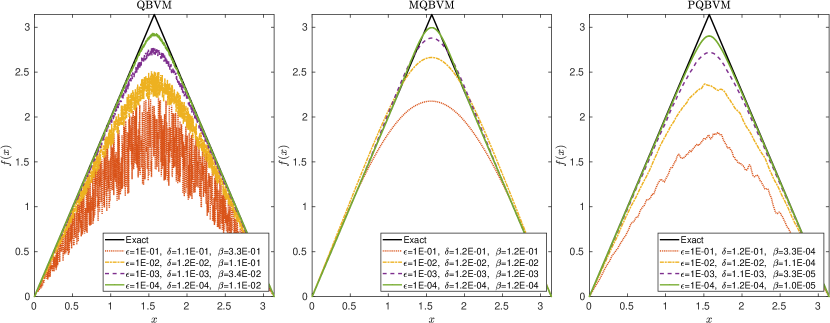
Figure 3: Reconstructed $f(x)$ in Ex. 2 with different methods and noise levels $\epsilon\in\{10^{-1},10^{-2},10^{-3},10^{-4}\}$ (using the mesh $h=\pi/1024,\tau=T/1024$, $\alpha=\delta^{1/2}$ for QBVM, $\alpha=\delta$ for MQBVM, and $\alpha=\tau\delta^{1/2}$ for PQBVM). The black solid curve is the exact solution.

Table 3: Error and CPU results for Ex. 3 with different mesh sizes and noise levels.

		Errors in $L_{2}$ norm				CPU (in seconds)
Method	$(m,n)$$\backslash$ $\epsilon$	$10^{-1}$	$10^{-2}$	$10^{-3}$	$10^{-4}$	$10^{-1}$	$10^{-2}$	$10^{-3}$	$10^{-4}$
QBVM ($\beta=\delta^{1/2}$)	(256, 256)	5.04e-01	3.53e-01	2.55e-01	1.91e-01	0.5	0.5	0.5	0.5
	(512, 512)	5.21e-01	3.58e-01	2.58e-01	1.91e-01	2.6	2.5	2.6	2.5
	(1024,1024)	5.25e-01	3.57e-01	2.57e-01	1.92e-01	18.4	18.2	18.3	18.4
MQBVM ($\beta=\delta$)	(256, 256)	5.22e-01	3.42e-01	2.64e-01	1.97e-01	0.1	0.1	0.1	0.1
	(512, 512)	5.18e-01	3.40e-01	2.65e-01	1.97e-01	0.3	0.3	0.3	0.3
	(1024,1024)	5.16e-01	3.42e-01	2.63e-01	1.97e-01	1.3	1.3	1.3	1.3
PQBVM ($\beta=\tau\delta^{1/2}$)	(256, 256)	5.15e-01	3.68e-01	2.84e-01	2.34e-01	0.1	0.1	0.1	0.1
	(512, 512)	4.97e-01	3.61e-01	2.73e-01	2.19e-01	0.3	0.3	0.3	0.3
	(1024,1024)	4.97e-01	3.53e-01	2.65e-01	2.09e-01	1.2	1.2	1.3	1.2

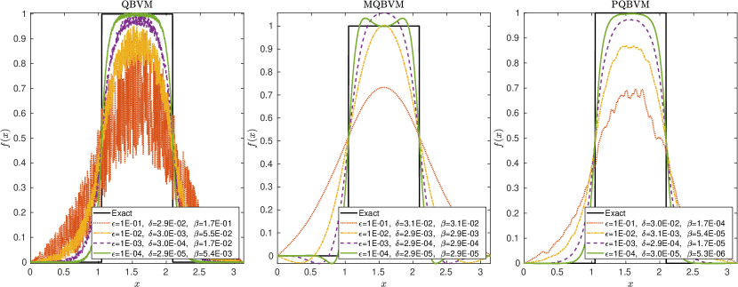
Figure 4: Reconstructed $f(x)$ in Ex. 3 with different methods and noise levels $\epsilon\in\{10^{-1},10^{-2},10^{-3},10^{-4}\}$ (using the mesh $h=\pi/1024,\tau=T/1024$, $\alpha=\delta^{1/2}$ for QBVM, $\alpha=\delta$ for MQBVM, and $\alpha=\tau\delta^{1/2}$ for PQBVM). The black solid curve is the exact solution.

Example 3. Choose $\Omega=(0,\pi),T=1$, $\phi(x)=0$, and a discontinuous source function

$$f(x)=\begin{cases}1,&\pi/3\leq x\leq 2\pi/3,\\ 0,&\mathrm{else},\\ \end{cases}$$

Table 3 reports the error results and CPU times with three different regularization methods, where the errors of all three methods are comparable but the CPU times of both MQBVM and PQBVM based on our PinT direct solver are much faster. Figure 4 illustrates the reconstructed $f(x)$ with different noise levels, where the MQBVM shows more clear Gibbs phenomenon due to discontinuity and the PQBVM seems to provide most stable approximation in the sense of avoiding oscillations and overshooting near the discontinuities.

Table 4: Error and CPU results for 2D Ex. 4 with different mesh sizes and noise levels.

		Errors in $L_{2}$ norm			CPU (in seconds)
Method	$(m,n)$$\backslash$ $\epsilon$	$10^{-1}$	$10^{-2}$	$10^{-3}$	$10^{-1}$	$10^{-2}$	$10^{-3}$
QBVM ($\beta=\delta^{1/2}$)	($32^{2}$, 32)	2.21e+00	1.18e+00	4.98e-01	2.00	2.09	2.08
	($64^{2}$, 64)	2.21e+00	1.18e+00	4.93e-01	132.01	127.05	132.84
	($128^{2}$, 128)	–	–	–	–	–	–
MQBVM ($\beta=\delta$)	($32^{2}$, 32)	3.26e+00	2.20e+00	9.83e-01	0.01	0.01	0.01
	($64^{2}$, 64)	3.26e+00	2.21e+00	9.82e-01	0.04	0.04	0.05
	($128^{2}$, 128)	3.26e+00	2.20e+00	9.85e-01	0.28	0.29	0.28
	($256^{2}$, 256)	3.26e+00	2.20e+00	9.84e-01	2.83	2.90	2.91
	($512^{2}$, 512)	3.26e+00	2.20e+00	9.84e-01	33.68	33.80	33.56
PQBVM ($\beta=\tau\delta^{1/2}$)	($32^{2}$, 32)	2.53e+00	1.72e+00	1.19e+00	0.01	0.01	0.01
	($64^{2}$, 64)	2.39e+00	1.49e+00	8.92e-01	0.04	0.04	0.04
	($128^{2}$, 128)	2.31e+00	1.35e+00	7.05e-01	0.29	0.28	0.28
	($256^{2}$, 256)	2.26e+00	1.27e+00	6.04e-01	3.41	2.92	3.44
	($512^{2}$, 512)	2.23e+00	1.23e+00	5.49e-01	34.42	33.96	33.72

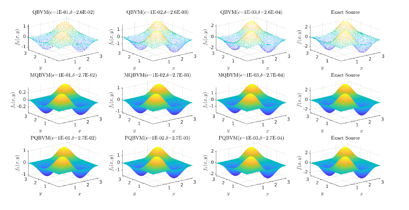
Figure 5: Reconstructed $f(x)$ in Ex. 4 with different methods and noise levels $\epsilon\in\{10^{-1},10^{-2},10^{-3}\}$ (using the mesh $h=\pi/512,\tau=T/512$, $\alpha=\delta^{1/2}$ for QBVM, $\alpha=\delta$ for MQBVM, and $\alpha=\tau\delta^{1/2}$ for PQBVM).

Example 4. Choose $\Omega=(0,\pi)^{2},T=1$, $\phi(x,y)=0$, and a smooth source function

$$f(x,y)=x(\pi-x)\sin(2x)y(\pi-y)\cos(y).$$

Table 4 reports the error results and CPU times with three different regularization methods, where the CPU times of both MQBVM and PQBVM based on our PinT direct solver are much faster although the errors of QBVM are slightly smaller than MQBVM and PQBVM. Notice that even for a small mesh size $(m,n)=(64^{2},64)$ the CPU times are decreased from over 2 mins to about $0.04$ second, let alone a larger mesh size (such as $(m,n)=(128^{2},128)$ with about 2.1 million unknowns). Here we used “–” to indicate the computation takes an excessively long time for MATLAB’s backslash sparse direct solver. Figure 5 illustrates the reconstructed $f(x)$ with different noise levels, where the differences between three methods are not clearly visible. This example demonstrates the superior computational efficiency of our proposed PinT direct solver in treating more practical 2D/3D problems that are costly to solve by the sparse direct solver.

5.2 Application to separable space and time-dependent source term

Consider the following model [20] with a given positive time-dependent source term $q(t)>0$:

$$\begin{array}[]{lllllllll}\left\{\begin{array}[]{ll}u_{t}-\Delta u=f(x)q(t),&\quad\textnormal{in}\quad\Omega\times(0,T),\\ u(\cdot,t)=0,&\quad\textnormal{on}\quad\partial\Omega\times(0,T),\\ u(\cdot,0)=\phi,&\quad\textnormal{in}\quad\Omega,\\ u(\cdot,T)+{\beta(\alpha f(\cdot)-\Delta f(\cdot)})=g_{\delta},&\quad\textnormal{in}\quad\Omega.\end{array}\right.\end{array}$$ (54)

With the same finite-difference discretization, we get a linear system of Kronecker product form

$$A_{h}=B_{q}\otimes I_{h}-I_{t}\otimes\Delta_{h}$$ (55)

where the time discretization matrix $B_{q}$ is given by (let $q_{j}=q(t_{j})$)

$$B_{q} =\left[\begin{array}[]{ccccccccc}\alpha&0&0&\cdots&0&1/\beta\\ -q_{1}&1/\tau&0&\cdots&0&0\\ -q_{2}&-1/\tau&1/\tau&0&\cdots&0\\ \vdots&0&\ddots&\ddots&\ddots&0\\ -q_{n-1}&0&\cdots&-1/\tau&1/\tau&0\\ -q_{n}&0&\cdots&0&-1/\tau&1/\tau\end{array}\right]\in{\mathbb{R}}^{(n+1)\times(n+1)}.$$ (62)

Hence, our proposed direct PinT solver can still be applied if assuming $B_{q}=V_{q}D_{q}V_{q}^{-1}$ is diagonalizable and $V_{q}$ is somewhat well-conditioned. In this case, the diagonalizability of $B_{q}$ and the estimate of $\kappa(V_{q})$ are much more complicated to discuss as we did for the $B$ with $q(t)\equiv 1$, which will be left as future work. The following example shows numerically it indeed works very well.

Example 5. Choose $\Omega=(0,\pi),T=1$, $\phi(x)=0$, and the smooth source functions

$$f(x)=x(\pi-x)\sin(4x),\qquad g(t)=e^{-t}+\ln(t+1)+t^{2}.$$

Table 5 reports the error results and CPU times with three different regularization methods as before and Figure 6 compares the reconstructed $f$, where similar conclusions can be made as in the previous Example 1. The extra non-constant $q(t)$ term does not seems to affect the effectiveness of our proposed method, although our current analysis does not fully support this case yet.

Table 5: Error and CPU results for Ex. 5 with different mesh sizes and noise levels.

		Errors in $L_{2}$ norm				CPU (in seconds)
Method	$(m,n)$$\backslash$ $\epsilon$	$10^{-1}$	$10^{-2}$	$10^{-3}$	$10^{-4}$	$10^{-1}$	$10^{-2}$	$10^{-3}$	$10^{-4}$
QBVM ($\beta=\delta^{1/2}$)	(256, 256)	1.23e+00	6.27e-01	2.60e-01	8.50e-02	0.5	0.5	0.5	0.5
	(512, 512)	1.24e+00	6.32e-01	2.58e-01	9.03e-02	2.5	2.5	2.5	2.5
	(1024,1024)	1.23e+00	6.39e-01	2.54e-01	9.13e-02	18.3	18.1	18.0	18.2
MQBVM ($\beta=\delta$)	(256, 256)	1.61e+00	5.29e-01	1.07e-01	1.44e-02	0.1	0.1	0.1	0.1
	(512, 512)	1.62e+00	5.73e-01	1.02e-01	1.56e-02	0.3	0.3	0.3	0.3
	(1024,1024)	1.62e+00	5.73e-01	1.03e-01	1.58e-02	1.3	1.3	1.3	1.3
PQBVM ($\beta=\tau\delta^{1/2}$)	(256, 256)	1.28e+00	6.94e-01	3.27e-01	1.61e-01	0.1	0.1	0.1	0.1
	(512, 512)	1.25e+00	6.62e-01	2.92e-01	1.27e-01	0.3	0.3	0.3	0.3
	(1024,1024)	1.25e+00	6.53e-01	2.79e-01	1.10e-01	1.3	1.2	1.4	1.3

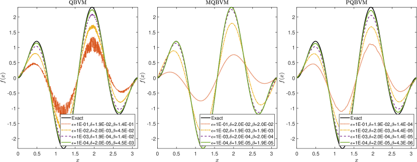
Figure 6: Reconstructed $f(x)$ in Ex. 5 with different methods and noise levels $\epsilon\in\{10^{-1},10^{-2},10^{-3},10^{-4}\}$ (using the mesh $h=\pi/1024,\tau=T/1024$, $\alpha=\delta^{1/2}$ for QBVM, $\alpha=\delta$ for MQBVM, and $\alpha=\tau\delta^{1/2}$ for PQBVM). The black solid curve is the exact solution.

6 Conclusions

Inverse source problems are ill-posed and effective regularization is required for their stable numerical computation. The quasi-boundary value method and its variants are often used for regularizing such problems, which lead to large-scale ill-conditioned nonsymmetric sparse linear systems upon suitable space-time finite difference discretization. Such nonsymmetric all-at-once linear systems are costly to solve by either direct or iterative methods. In this paper we propose to modify the existing quasi-boundary value methods such that the full discretized system matrix admits a block Kronecker sum structure that can be solved by a fast diagonalization-based PinT direct solver. To control the roundoff errors of such a PinT direct solver, we carefully estimate the condition number of the eigenvector matrix of the time discretization matrix, where the free parameter $\alpha=\alpha_{*}$ is determined for this purpose. Convergence analysis (with a priori choice of regularization parameter $\beta$) for our proposed parameterized quasi-boundary value method (PQBVM) is given under the special choice of $\alpha=\alpha_{*}$. Both 1D and 2D examples show our proposed PinT methods can achieve a comparable accuracy with significantly faster CPU times. It is interesting to generalize our idea of integrating regularization and fast solvers to other related inverse PDE problems, such as to simultaneously recover the source term and initial value [17, 39, 54, 37, 38].

References

- [1] M. N. Ahmadabadi, M. Arab, and F. M. Ghaini, The method of fundamental solutions for the inverse space-dependent heat source problem, Engineering Analysis with Boundary Elements, 33 (2009), pp. 1231–1235.
- [2] M. Ali, S. Aziz, and S. A. Malik, Inverse source problems for a space–time fractional differential equation, Inverse Problems in Science and Engineering, 28 (2020), pp. 47–68.
- [3] G. Caklovic, R. Speck, and M. Frank, A parallel implementation of a diagonalization-based parallel-in-time integrator, arXiv preprint arXiv:2103.12571, (2021).
- [4] J. R. Cannon and P. DuChateau, Structural identification of an unknown source term in a heat equation, Inverse Problems, 14 (1998), pp. 535–551.
- [5] D. S. Daoud, Stability of the parareal time discretization for parabolic inverse problems, in Domain decomposition methods in science and engineering XVI, Springer, 2007, pp. 275–282.
- [6] F.-F. Dou, C.-L. Fu, and F. Yang, Identifying an unknown source term in a heat equation, Inverse Problems in Science and Engineering, 17 (2009), pp. 901–913.
- [7] F.-F. Dou, C.-L. Fu, and F.-L. Yang, Optimal error bound and Fourier regularization for identifying an unknown source in the heat equation, Journal of computational and applied mathematics, 230 (2009), pp. 728–737.
- [8] H. Engl, M. Hanke, and A. Neubauer, Regularization of Inverse Problems, Mathematics and Its Applications, Springer Netherlands, 2000.
- [9] A. Farcas and D. Lesnic, The boundary-element method for the determination of a heat source dependent on one variable, Journal of Engineering Mathematics, 54 (2006), pp. 375–388.
- [10] A. Fatullayev, Numerical solution of the inverse problem of determining an unknown source term in a heat equation., Mathematics and Computers in Simulation, 58 (2002), pp. 247–253.
- [11] , Numerical solution of the inverse problem of determining an unknown source term in a two-dimensional heat equation., Applied mathematics and computation, 152 (2004), pp. 659–666.
- [12] M. J. Gander, 50 years of time parallel time integration, in Multiple shooting and time domain decomposition methods, Springer, 2015, pp. 69–113.
- [13] M. J. Gander, L. Halpern, J. Rannou, and J. Ryan, A direct time parallel solver by diagonalization for the wave equation, SIAM J. Sci. Comput., 41 (2019), pp. A220–A245.
- [14] G. Golub, M. Heath, and G. Wahba, Generalized cross-validation as method for choosing a good ride parameter., Technometrics, 2 (1979).
- [15] B. Jin and W. Rundell, A tutorial on inverse problems for anomalous diffusion processes, Inverse problems, 31 (2015), p. 035003.
- [16] B. T. Johansson and D. Lesnic, A variational method for identifying a spacewise-dependent heat source, IMA Journal of Applied Mathematics, 72 (2007), pp. 748–760.
- [17] , A procedure for determining a spacewise dependent heat source and the initial temperature, Applicable Analysis, 87 (2008), pp. 265–276.
- [18] T. Johansson and D. Lesnic, Determination of a spacewise dependent heat source, Journal of computational and Applied Mathematics, 209 (2007), pp. 66–80.
- [19] S. I. Kabanikhin, Inverse and ill-posed problems, de Gruyter, 2011.
- [20] R. Ke, M. K. Ng, and T. Wei, Efficient preconditioning for time fractional diffusion inverse source problems, SIAM Journal on Matrix Analysis and Applications, 41 (2020), pp. 1857–1888.
- [21] A. Kirsch, An introduction to the mathematical theory of inverse problems, vol. 120, Springer Nature, 2021.
- [22] J. Lee and D. Sheen, A parallel method for backward parabolic problems based on the Laplace transformation, SIAM journal on numerical analysis, 44 (2006), pp. 1466–1486.
- [23] D. Lesnic, Inverse Problems with Applications in Science and Engineering, CRC Press, 2021.
- [24] J. Liu, Fast parallel-in-time quasi-boundary value methods for backward heat conduction problems, arXiv preprint arXiv:2107.06381, (2021).
- [25] J. Liu and Z. Wang, A ROM-accelerated parallel-in-time preconditioner for solving all-at-once systems in unsteady convection-diffusion PDEs, Applied Mathematics and Computation, 416 (2022), p. 126750.
- [26] J. Liu and S. L. Wu, A fast block -circulant preconditoner for all-at-once systems from wave equations, SIAM J. Matrix Anal. Appl., 41 (2020), pp. 1912–1943.
- [27] J. Liu and M. Xiao, Quasi-boundary value methods for regularizing the backward parabolic equation under the optimal control framework, Inverse Problems, 35 (2019), p. 124003.
- [28] Y. Ma, C. Fu, and Y. Zhang, Identification of an unknown source depending on both time and space variables by a variational method., Applied Mathematical Modelling., 36 (2012), pp. 5080–5090.
- [29] Y. Maday and E. M. Rønquist, Parallelization in time through tensor-product space-time solvers, C. R. Acad. Sci. Paris Sér. I Math., 346 (2008), pp. 113–118.
- [30] E. McDonald, J. Pestana, and A. Wathen, Preconditioning and iterative solution of all-at-once systems for evolutionary partial differential equations, SIAM J. Sci. Comput., 40 (2018), pp. A1012–A1033.
- [31] H. T. Nguyen, D. L. Le, et al., Regularized solution of an inverse source problem for a time fractional diffusion equation, Applied Mathematical Modelling, 40 (2016), pp. 8244–8264.
- [32] E. G. SAVATEEV, On problems of determining the source function in a parabolic equation, Journal of Inverse and Ill-Posed Problems, 3 (1995).
- [33] T. I. Seidman, Optimal filtering for the backward heat equation, SIAM Journal on Numerical Analysis, 33 (1996), pp. 162–170.
- [34] U. Tautenhahn and T. Schröter, On optimal regularization methods for the backward heat equation, Zeitschrift für Analysis und ihre Anwendungen, 15 (1996), pp. 475–493.
- [35] D. Trong, N. Long, and P. Alain, Nonhomogeneous heat equation: Identification and regularization for the inhomogeneous term., Journal of mathematical analysis and applications, 312 (2005), pp. 93–104.
- [36] D. Trong, P. Quan, and P. Alain, Determination of a two-dimensional heat source: uniqueness, regularization and error estimate., Journal of computational and applied mathematics, 191 (2006), pp. 50–67.
- [37] B. Wang, B. Yang, and M. Xu, Simultaneous identification of initial field and spatial heat source for heat conduction process by optimizations, Advances in Difference Equations, 2019 (2019), pp. 1–16.
- [38] Z. Wang, S. Chen, S. Qiu, and B. Wu, A non-iterative method for recovering the space-dependent source and the initial value simultaneously in a parabolic equation, Journal of Inverse and Ill-posed Problems, 28 (2020), pp. 499–516.
- [39] Z. Wang, S. Qiu, Z. Ruan, and W. Zhang, A regularized optimization method for identifying the space-dependent source and the initial value simultaneously in a parabolic equation, Computers & Mathematics with Applications, 67 (2014), pp. 1345–1357.
- [40] Z. Wang, W. Zhang, and B. Wu, Regularized optimization method for determining the space-dependent source in a parabolic equation without iteration., Journal of Computational Analysis & Applications., 20 (2016).
- [41] T. Wei, X. Li, and Y. Li, An inverse time-dependent source problem for a time-fractional diffusion equation, Inverse Problems, 32 (2016), p. 085003.
- [42] T. Wei and J. Wang, A modified quasi-boundary value method for an inverse source problem of the time-fractional diffusion equation, Applied Numerical Mathematics, 78 (2014), pp. 95–111.
- [43] T. Wei and J.-G. Wang, A modified quasi-boundary value method for the backward time-fractional diffusion problem, ESAIM: Mathematical Modelling and Numerical Analysis, 48 (2014), pp. 603–621.
- [44] S.-L. Wu and J. Liu, A parallel-in-time block-circulant preconditioner for optimal control of wave equations, SIAM Journal on Scientific Computing, 42 (2020), pp. A1510–A1540.
- [45] L. Yan, C.-L. Fu, and F.-F. Dou, A computational method for identifying a spacewise-dependent heat source., International Journal for Numerical Methods in Biomedical Engineering., 26 (2010), pp. 597–608.
- [46] L. Yan, C.-L. Fu, and F.-L. Yang, The method of fundamental solutions for the inverse heat source problem, Engineering Analysis with Boundary Elements, 32 (2008), pp. 216–222.
- [47] L. Yan, F.-L. Yang, and C.-L. Fu, A meshless method for solving an inverse spacewise-dependent heat source problem, Journal of Computational Physics, 228 (2009), pp. 123–136.
- [48] F. Yang and C.-L. Fu, A simplified Tikhonov regularization method for determining the heat source, Applied Mathematical Modelling, 34 (2010), pp. 3286–3299.
- [49] F. Yang, C.-L. Fu, and X.-X. Li, A quasi-boundary value regularization method for determining the heat source, Mathematical Methods in the Applied Sciences, 37 (2013), pp. 3026–3035.
- [50] F. Yang, C.-L. Fu, and X.-X. Li, The inverse source problem for time-fractional diffusion equation: stability analysis and regularization, Inverse Problems in Science and Engineering, 23 (2015), pp. 969–996.
- [51] L. Yang, M. Dehghan, J. Yu, and G. Luo, Inverse problem of time-dependent heat sources numerical reconstruction., Mathematics and Computers in Simulation., 81 (2011), pp. 1656–1672.
- [52] L. Yang, J. Yu, G. Luo, and Z. Deng, Numerical identification of source terms for a two dimensional heat conduction problem in polar coordinate system., Applied Mathematical Modelling., 37 (2013), pp. 939–957.
- [53] Z. Yi and D. Murio, Source term identification in 1D IHCP., Computers & Mathematics with Applications., 47 (2004), pp. 1921–1933.
- [54] G.-H. Zheng and T. Wei, Recovering the source and initial value simultaneously in a parabolic equation, Inverse Problems, 30 (2014), p. 065013.