The First Near-Infrared Transmission Spectrum of HIP 41378 f,
a Low-Mass Temperate Jovian World in a Multi-Planet System

Abstract

We present a near-infrared transmission spectrum of the long period (P=542 days), temperate ($\rm T_{eq}$=294 K) giant planet HIP 41378 $\rm f$ obtained with the Wide-Field Camera 3 (WFC3) instrument aboard the Hubble Space Telescope (HST). With a measured mass of $12\pm 3$ $M_{\earth}$ and a radius of $9.2\pm 0.1$ $R_{\earth}$, HIP 41378 $\rm f$ has an extremely low bulk density ($0.09\pm 0.02\,{\rm g}\,{\rm cm}^{-3}$). We measure the transit depth with a median precision of 84 ppm in 30 spectrophotometric channels with uniformly-sized widths of 0.018 $\mu$m. Within this level of precision, the spectrum shows no evidence of absorption from gaseous molecular features between 1.1–1.7 $\mu$m. Comparing the observed transmission spectrum to a suite of 1D radiative-convective-thermochemical-equilibrium forward models, we rule out clear, low-metallicity atmospheres and find that the data prefer high-metallicity atmospheres or models with an additional opacity source, such as high-altitude hazes and/or circumplanetary rings. We explore the ringed scenario for HIP 41378 $\rm f$ further by jointly fitting the K2 and HST light curves to constrain the properties of putative rings. We also assess the possibility of distinguishing between hazy, ringed, and high-metallicity scenarios at longer wavelengths with JWST. HIP 41378 $\rm f$ provides a rare opportunity to probe the atmospheric composition of a cool giant planet spanning the gap in temperature, orbital separation, and stellar irradiation between the Solar System giants, directly imaged planets, and the highly-irradiated hot Jupiters traditionally studied via transit spectroscopy.

1 Introduction

The Solar System gas and ice giants host ring systems, although the origins of these rings remain mysterious (e.g., De Pater et al. 2018a, b; Hedman & Chancia 2021). Whereas Saturn’s massive rings are rich in water ice (Cuzzi & Estrada 1998; Poulet et al. 2003; Nicholson et al. 2005), the less massive rings of Uranus and Neptune have a higher content of rocky particles (Tiscareno et al. 2013) and Jupiter’s tenuous rings are composed of micron-sized dust particles (De Pater et al. 2018a). Massive ring systems like that of Saturn’s may form from collisions (e.g., Pollack 1975), or tidal disruptions of primordial satellites (Canup 2010) or passing objects (e.g., Dones 1991). Despite the prevalence of rings around the Solar System giants, exoplanet characterization efforts have not yet yielded conclusive observational evidence of circumplanetary rings (Heising et al. 2015; Aizawa et al. 2018). The presence of ring systems around giant exoplanets, however, may explain planets with large measured radii and unusually low bulk densities.

HIP 41378 is a nearby bright ($V=8.93$), late F-type star hosting five transiting planets (Vanderburg et al. 2016; Berardo et al. 2019). With $\rm T_{eq}$=294 K (assuming full heat redistribution and zero Bond albedo), the outermost HIP 41378 $\rm f$ is an intriguing target for atmospheric characterization because it is significantly colder than the giant exoplanets typically probed by ground-based and space-based observations. It therefore provides a bridge between the highly-irradiated hot Jupiters studied via transmission spectroscopy; the young, wide-orbit, and massive giant planets or substellar objects studied via direct imaging; and the colder, mature gas giants in the Solar System. With a measured mass of 12$\pm$3 $M_{\earth}$ and a radius of 9.2$\pm$0.1 $R_{\earth}$ (Santerne et al., 2019), HIP 41378 $\rm f$ stands out as one of the lowest bulk density planets discovered to date ($0.09\pm 0.02\,{\rm g}\,{\rm cm}^{-3}$).

Rings have been shown theoretically to inflate an exoplanet’s radius measured through transits, thereby decreasing the inferred bulk density (Piro & Vissapragada, 2020; Akinsanmi et al., 2020). As discussed in Akinsanmi et al. (2020), the ring-induced transit depth enhancement is expected to be chromatic: deeper transits occur at wavelengths where the ring is optically thick. Based on detailed modeling of the observed K2 photometry, the most likely ring scenario for HIP 41378 $\rm f$ is a Uranian-like bulk density of 1.23 ${\rm g}\,{\rm cm}^{-3}$ and a ring extending from 1.05 to 2.59 times the planetary radius inclined at an angle of $\sim$25^∘ from the sky plane (Akinsanmi et al., 2020). While HIP 41378 $\rm f$ is too close to its host star to support icy rings, the planet could instead be orbited by rings composed of small, porous rocky particles (Piro & Vissapragada, 2020; Akinsanmi et al., 2020). In this ringed model, the planet radius would be $\rm R_{p}=3.7\pm 0.3\,\rm R_{\oplus}$ (compared to $\rm R_{p}=9.21\pm 0.01\,\rm R_{\oplus}$ for the ringless case).

Alternatively, if HIP 41378 $\rm f$ does not possess rings, then it may be a member of the rare class of “super-puff” exoplanets, which have been inferred to possess gas mass fractions far greater than the more common mini-Neptunes with similiar masses ($>$10% vs. a few %, respectively; Lopez & Fortney 2014). Super-puffs have been hypothesized to form in a less opaque region of the protoplanetary disk (Lee & Chiang, 2016), followed by inward migration to account for their large gas mass fractions. However, despite their low densities and correspondingly large atmospheric scale heights, all transmission spectra of super-puffs observed to date have been flat (e.g., Libby-Roberts et al. 2020; Chachan et al. 2020), suggesting that flat spectra are a general property of the population. High-altitude photochemical hazes have been considered to explain both the flat spectra and the large radii of super-puffs (Gao & Zhang 2020; Ohno & Tanaka 2021), although dusty outflows driven by expected high mass loss rates (Wang & Dai, 2019) may also explain their effective radii.

Here we present the near-infrared transmission spectrum of HIP 41378 $\rm f$ obtained with the Hubble Space Telescope Wide-Field Camera 3 (HST/WFC3), which we use to constrain the planet’s atmospheric composition and explore the presence of circumplanetary rings. In Section 2, we describe our HST observations and data reduction procedure. Section 3 details our methods for fitting the transit light curves. In Section 4, we present the near-infrared transmission spectrum of HIP 41378 $\rm f$. In Section 5, we interpret our results using atmospheric models, explore the possibility of rings, and compare HIP 41378 $\rm f$ to other planets with similar masses and radii. Section 6 summarizes our results.

2 Observations & Data Reduction

2.1 Observations

We observed a single primary transit of HIP 41378 $\rm f$ with HST/WFC3 using the G141 grism, which provides spectroscopy between 1.125-1.643 $\mu$m at a spectral resolving power of R$\sim$130 around $\lambda$=1.4 $\mu$m. Taken as part of GO 16267 (PI: Dressing) on UT 2021 May 19-21, the observations were scheduled over three consecutive HST visits of six orbits each to accommodate the target’s long transit duration (18.998 hours; Vanderburg et al. 2016). To ensure that the target remained centered in the instrument’s field of view, we took an image of the target using the F126N filter with an exposure time of 7.317 seconds at the beginning of the first and third visits as well as at the beginning of the last orbit of the second visit. We then obtained time series spectroscopy with the G141 grism, and used round-trip spatial scanning for all visits with a scan rate of 0.419 arcsec s^-1 to permit taking longer exposures without saturating the detector (McCullough & MacKenty, 2012).

Due to South Atlantic Anomaly (SAA) passages during the transit, we varied the sampling sequence for affected orbits. The first three were impacted by SAA passages, making roughly half, a third, and a quarter of the respective orbits unusable. The fourth through tenth orbits were less affected, so we were able to use almost all exposures taken during these orbits. For the remaining orbits (orbits 11-18), we again faced interruptions due to the SAA. Ultimately, we used the SPARS10 sampling sequence with 7-9 non-destructive reads per exposure (NSAMP = 7-9). As a result of these NSAMP changes, the total integration times ranged from 37.010 to 51.703 seconds and scans were taken across approximately 126-178 pixel rows in the cross-dispersion direction. With this instrument setup, we read out a 512$\times$512 pixel subarray for each science exposure and obtained a total of 274 science exposures over the 18 orbits observed.

2.2 Data Reduction

We reduced the observations for this program using the methods outlined in Alam et al. (2020), which we briefly summarize here. We started our analysis using the bias-corrected, flat-fielded ima images from the CALWF3 pipeline. The flux for each exposure was extracted by taking the difference between successive reads and then performing a background subtraction to suppress contamination from nearby stars. For the background subtraction, we subtracted the median flux from a box 32 pixels away from the spectrum. To correct for cosmic ray events, we followed the procedure of Nikolov et al. (2014).

Next, we extracted stellar spectra by summing the flux within a rectangular aperture. To determine the size of the aperture (accounting for the different-sized spatial scans; see Section 2.1), we fit for the aperture width along the dispersion and cross-dispersion axes. We scanned each row of the raw ima images and fit a top-hat function to the data to determine the center of the PSF (i.e., the center of the 2D spectrum along the cross-dispersion axis). To determine the center of the spectrum along the dispersion direction, we scanned each column and fit a top-hat distribution to the data. We then used these fitted x and y center points as initial guesses for calculating the centroid positions on each image using the flux-weighted first moments in x and y pixel position. To determine the wavelength solution, we cross-correlated each stellar spectrum to a grid of model spectra from the WFC3 Exposure Time Calculator (ETC) with temperatures ranging from 4060-9230 K. To determine shifts along the dispersion axis, we used the closest matching model of 6200 K. The final wavelengths assigned to each element of the spectrum are the wavelengths from the ETC model with the shift applied.

3 Light Curve Fits

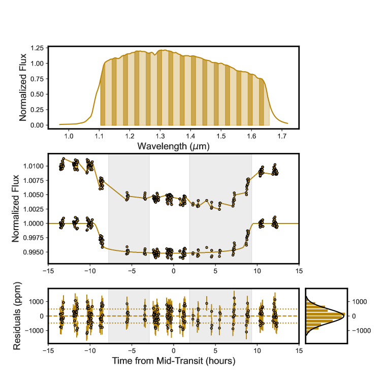
Figure 1: Top: Example HIP 41378 $\rm f$ stellar spectrum for the HST/WFC3 G141 grism. The vertical bands denote the 0.018 $\mu$m wavelength channels adopted for the spectroscopic light curves. Middle: Raw (top) and detrended (bottom) white light curve, excluding the first orbit and the first exposure of each subsequent orbit (points). The raw light curve has been shifted vertically by an arbitrary constant for clarity. Overplotted is the best-fitting analytic light curve model (line). Epochs most affected by South Atlantic Anomaly passages are denoted by the gray shading. Bottom: RMS residuals of the transit fit in ppm (left; points) and 1-$\sigma$ range of the residuals (dotted lines), as well as the the distribution of residuals (right).

To extract the 1.1-1.7 $\mu$m transmission spectrum, we fit the transit light curves using the fitting routine detailed in Kirk et al. (2017, 2018, 2019, 2021) and Alam et al. (2021). Briefly, we modeled the analytic transit light curves (Mandel & Agol, 2002) using Batman (Kreidberg, 2015) and implemented a Gaussian process (GP) with the george code (Ambikasaran et al., 2015) to model noise in the data. We fixed the non-linear limb darkening coefficients to the theoretical values from 3D stellar models (Magic et al., 2015), assuming stellar properties consistent with Santerne et al. (2019) ($\rm T_{eff}$=6320 K, log(g)=4.294, [Fe/H]=-0.1).

To fit the white light curve (1.104-1.661 $\mu$m), we fixed the system parameters to those in Santerne et al. 2019 ($\rm P$=542.07975 days, $\rm a/R_{\star}$=231.417, $i$=89.971^∘, $e$=0). We fit for the time of mid-transit $\rm T_{0}$, the scaled planetary radius $\rm R_{p}/R_{\star}$, and the GP hyperparameters. For the white light curve, we used three squared-exponential GP kernels with the orbital phase of HST, the wavelength shift in the stellar spectra, and time as the three input vectors – after standardizing each (subtracting the mean and dividing by the standard deviation to put each on a common scale). We fit for the natural logarithm of the inverse length-scale for each kernel, in addition to the amplitude of the GP and a white noise term. The GP was therefore described by five free hyperparameters. We placed truncated uniform-in-log-space priors on the GP hyperparameters. The amplitude was bounded between 0.01 and $100\times$ the out-of-transit variance and the length scales were bounded between the minimum spacing and $3\times$ the maximum spacing of the standardized input vectors. The white noise term was bounded between 0.1 and 1000 ppm.

To sample the parameter space for the white light curve and spectroscopic light curves, we ran a Markov Chain Monte Carlo (MCMC) using emcee after clipping $>$4-$\sigma$ outliers from a running median computed for each light curve, which clipped 0–2 points per light curve. We optimized the GP hyperparameters to the out-of-transit data to find the starting locations for the hyperparameters. We followed the example in the george documentation and used scipy.optimize (Jones et al., 2001) and a ‘L-BFGS-B’ algorithm to perform the optimization of the GP hyperparameters. The starting value for $\rm R_{p}/R_{\star}$ was taken to be 0.0663 (Santerne et al., 2019) and the starting $\rm T_{0}$ value of BJD 2459354.6 was determined by visual inspection of the light curve. We initialized the chains around these values and ran the MCMC with 210 walkers for a 2000 step burn-in, followed by a 6000 step chain for our posterior and parameter estimates. The number of samples was $72\times$ the autocorrelation length, greater than the $50\times$ autocorrelation length which in general indicates convergence in emcee. The best-fit white light curve is shown in Figure 1, with $\rm R_{p}/R_{\star}$ = 0.068602 ${}^{+0.002684}_{-0.003370}$ and $\rm T_{0}$ = BJD 2459355.101374 ${}^{+0.001919}_{-0.001888}$.

For the binned light curve fits, we used a common mode correction. This correction involved removing the best-fitting white light systematics model and the residuals to the white light fit from each binned light curve prior to fitting (e.g., Gibson 2014; Alam et al. 2020). As a result, we were able to use a simpler systematics model for the binned light curves and therefore only used two GP kernels (HST phase and wavelength shift). We also held $\rm T_{0}$ fixed to the best-fit value from the white light curve fit, resulting in five free parameters per binned light curve ($\rm R_{p}/R_{\star}$ and the four GP hyperparameters). We then proceeded with the MCMC as for the white light curve fit. The measured $\rm R_{p}/R_{\star}$ values for each spectroscopic light curve are presented in Table 1.

4 Results

The near-infrared (1.1-1.7 $\mu$m) transmission spectrum of HIP 41378 $\rm f$ is shown in Figure 2. The $\rm R_{p}/R_{\star}$ values measured from our WFC3 transmission spectrum (Table 1) vary between 0.067 and 0.070, consistent within 2-$\sigma$ with the optical transit depths measured from the two K2 observations (0.0672$\pm$0.0013, Vanderburg et al. 2016; $0.06602^{+0.00017}_{-0.00016}$, Berardo et al. 2019; 0.0663$\pm$0.0001, Santerne et al. 2019). Within the precision of our observations, we find that the spectrum does not display any large absorption features from gaseous molecules, with maximum deviations spanning $\sim$2 scale heights (i.e., $\sim 1200$ km, assuming a H/He-dominated atmospheric composition with a mean molecular weight of 2.3 amu).

Figure 2: Broadband transmission spectrum for HIP 41378 $\rm f$ (black points), compared to 1D radiative-convective forward models (colored lines) for a clear atmosphere with metallicities 1$\times$, 30$\times$, and 300$\times$ solar, example hazy and ringed models, as well as a flat line (gray atmosphere). Top: The WFC3 transmission spectrum and the measured optical transit depth measurement from K2 (gray diamond; Santerne et al. 2019). Middle: Zoom-in to the WFC3 data presented in this work. Bottom: Zoom-out to the full spectrum, including mid-infrared wavelengths accessible with JWST.

Table 1: Broadband HST/WFC3 transmission spectrum for HIP 41378 f and adopted non-linear limb darkening coefficients

$\lambda$ ($\mu$m)	$\rm R_{p}/R_{*}$	$c_{1}$	$c_{2}$	$c_{3}$	$c_{4}$
1.104$-$1.122	0.067679 ${}^{+0.000692}_{-0.000693}$	0.6449	-0.2808	0.3552	-0.1548
1.122$-$1.141	0.068585 ${}^{+0.000635}_{-0.000637}$	0.6534	-0.3110	0.3794	-0.1639
1.141$-$1.159	0.068451 ${}^{+0.000580}_{-0.000598}$	0.6371	-0.2605	0.3191	-0.1396
1.159$-$1.178	0.068517 ${}^{+0.000584}_{-0.000587}$	0.6406	-0.2584	0.3035	-0.1340
1.178$-$1.196	0.068425 ${}^{+0.000524}_{-0.000528}$	0.6470	-0.2813	0.3155	-0.1335
1.196$-$1.215	0.068955 ${}^{+0.000606}_{-0.000617}$	0.6328	-0.2409	0.2684	-0.1154
1.215$-$1.233	0.068189 ${}^{+0.000606}_{-0.000605}$	0.6230	-0.1898	0.2075	-0.0945
1.233$-$1.252	0.069804 ${}^{+0.000593}_{-0.000607}$	0.6232	-0.1836	0.1922	-0.0884
1.252$-$1.271	0.068512 ${}^{+0.000536}_{-0.000550}$	0.6213	-0.1553	0.1457	-0.0694
1.271$-$1.289	0.068970 ${}^{+0.000650}_{-0.000659}$	0.6351	-0.1353	0.0720	-0.0408
1.289$-$1.308	0.068102 ${}^{+0.000553}_{-0.000549}$	0.6184	-0.1191	0.0842	-0.0426
1.308$-$1.326	0.068615 ${}^{+0.000569}_{-0.000561}$	0.6190	-0.1109	0.0633	-0.0320
1.326$-$1.345	0.068659 ${}^{+0.000529}_{-0.000532}$	0.6256	-0.1046	0.0418	-0.0232
1.345$-$1.364	0.069756 ${}^{+0.000577}_{-0.000587}$	0.6275	-0.0940	0.0124	-0.0081
1.364$-$1.382	0.068719 ${}^{+0.000621}_{-0.000618}$	0.6383	-0.0943	- 0.0114	0.0046
1.382$-$1.401	0.069385 ${}^{+0.000522}_{-0.000526}$	0.6424	-0.0831	- 0.0374	0.0160
1.401$-$1.419	0.068542 ${}^{+0.000518}_{-0.000519}$	0.6488	-0.0783	- 0.0556	0.0247
1.419$-$1.438	0.068728 ${}^{+0.000496}_{-0.000506}$	0.6495	-0.0572	- 0.1034	0.0495
1.438$-$1.456	0.068161 ${}^{+0.000640}_{-0.000645}$	0.6716	-0.1004	- 0.0728	0.0378
1.456$-$1.475	0.068362 ${}^{+0.000626}_{-0.000637}$	0.6829	-0.0861	- 0.1108	0.0554
1.475$-$1.494	0.068873 ${}^{+0.000534}_{-0.000532}$	0.6897	-0.1098	- 0.1023	0.0590
1.494$-$1.512	0.069306 ${}^{+0.000611}_{-0.000617}$	0.7115	-0.1676	- 0.0578	0.0451
1.512$-$1.531	0.068772 ${}^{+0.000615}_{-0.000620}$	0.7538	-0.2127	- 0.0480	0.0493
1.531$-$1.549	0.067925 ${}^{+0.000647}_{-0.000647}$	0.7838	-0.2858	0.0132	0.0297
1.549$-$1.568	0.067516 ${}^{+0.000636}_{-0.000646}$	0.7986	-0.3470	0.0823	0.0038
1.568$-$1.587	0.069565 ${}^{+0.000662}_{-0.000646}$	0.7781	-0.3858	0.1569	-0.0284
1.587$-$1.605	0.068607 ${}^{+0.000615}_{-0.000615}$	0.8379	-0.4884	0.2304	-0.0526
1.605$-$1.624	0.066955 ${}^{+0.000664}_{-0.000678}$	0.8540	-0.5049	0.2239	-0.0443
1.624$-$1.642	0.068270 ${}^{+0.000733}_{-0.000734}$	0.8801	-0.5741	0.2771	-0.0564
1.642$-$1.661	0.067865 ${}^{+0.000724}_{-0.000718}$	0.8508	-0.4979	0.2070	-0.0336

4.1 Comparisons to 1D Forward Models

We compare our observed transmission spectrum to model spectra generated using a 1D radiative-convective-thermochemical equilibrium model (Saumon & Marley, 2008) assuming clear, solar-composition atmospheres with metallicities 1$\times$, 30$\times$, and 300$\times$ solar. Considering HIP 41378 $\rm f$’s low bulk density and featureless transmission spectrum, we also compare to models incorporating high-altitude hazes and circumplanetary rings. The hazy models were computed using the Community Aerosol and Radiation Model for Atmospheres (CARMA; Gao et al., 2018) by adding a downward flux of haze particles to the 1$\times$ solar model atmosphere and tracking particle coagulation, sedimentation, and mixing (as in e.g., Adams et al. 2019). We assumed spherical haze particles with compositions of soots and tholins for haze column production fluxes of $10^{-10}$, $10^{-11}$, $10^{-12}$, $10^{-13}$, and $10^{-14}$ $\rm g~{}\rm cm^{-2}~{}\rm s^{-1}$ (Lavvas & Koskinen 2017; Kawashima & Ikoma 2019). We considered one soot model and one tholin model at each of the five haze production rates for a total of 10 hazy models.

We also computed transmission spectra with circumplanetary rings following the post-processing method described in a companion paper (Ohno & Fortney, 2022). In short, the method computes the spectrum by summing the transmittance of the ring-free planetary disk and the circumplanetary ring outside of the planetary disk. Using Equation 3 of Schlichting & Chang (2011), we estimate a minimum ring particle size of $\sim$10 cm and a system age of 3.1$\pm$0.6 Gyr (Santerne et al., 2019). Since the particle size is much larger than the relevant wavelength, we first assume a gray ring opacity. The gray rings model grid comprises 80 models assuming a solar composition atmosphere and an opaque ring with a morphology consistent with Akinsanmi et al. (2020). We varied the ring inclination between 21-28^∘ from the sky plane (in increments of 1^∘) and varied the inner ring radius between 1.02-1.11$\rm R_{0}$ (the ring-free transit radius of 0.35$\rm R_{J}$ from the clear 1$\times$ solar model, derived based on the measured mass from Santerne et al. 2019 and the inferred bulk density estimate from Akinsanmi et al. 2020) in steps of 0.01. The outer ring radius was fixed to 2.55$\rm R_{0}$, the Roche radius beyond which ring particles would coagulate into a satellite.

We also tested model grids for ring opacities computed using Mie theory and assuming a power-law size distribution for ring particles. The refractive indices are taken for astronomical silicates (Draine, 2003). We assumed a ring mass surface density of $100~{}{\rm g~{}{cm}^{-2}}$ with the largest particle size of $10\,{\rm m}$, similar to Saturnian rings. Since tiny particles might survive in optically thick rings (Schlichting & Chang, 2011), we set the smallest particle size to be $0.1~{}{\rm{\mu}m}$. We also tested the smallest sizes of $0.01$ and $1\,{\rm{\mu}m}$, but the results were almost unchanged. For all of the ringed models, the intrinsic atmospheric features are much smaller than those in ring-free scenario because the surface gravity is about 6 times higher than the ring-free scenario, significantly reducing the true atmospheric scale height and thus the spectral features.

We fit all of the models described above to the observed WFC3 transmission spectrum (excluding the K2 point) by computing the mean model prediction of each spectroscopic channel and performing a least-squares fit of the band-averaged model to the spectrum. In our fits, we preserved the shape of the model by allowing the vertical offset in $\rm R_{p}/R_{\star}$ between the spectrum and model to vary while holding all other parameters fixed. The number of degrees of freedom for each model is $n$ $-$ $m$, where $n$ is the number of data points and $m$ is the number of fitted parameters. Since $n$ = 30 for the HST spectrum and $m$ = 1, the number of degrees of freedom is the same for each model.

From the fits, we quantified our model selection by computing the $\chi_{r}^{2}$ statistic. Figure 2 shows the clear atmosphere models, the best-fitting hazy and ringed models, and a flat model. We rule out clear, low metallicity atmospheres ($\chi_{r}^{2}$=5.80 and 8.44 for the 1$\times$ and 30$\times$ solar cases, respectively). We cannot, however, distinguish between the high-metallicity (300$\times$ solar; $\chi_{r}^{2}$=1.84), hazy (soots, prod=$10^{-13}$ $\rm g~{}\rm cm^{-2}~{}\rm s^{-1}$; $\chi_{r}^{2}$=0.97), gray opacity ringed model ($\rm R_{in}$=$1.08\rm R_{0}$, $i_{\rm ring}$=28^∘; $\chi_{r}^{2}$=1.04) and non-gray ringed case ($\rm R_{in}$=$1.07\rm R_{0}$, $i_{\rm ring}$=28^∘, $\rm a_{max}$=10 $\mu$m; $\chi_{r}^{2}$=1.04) with the current observations. A flat spectrum (gray atmosphere) also matches the data well ($\chi_{r}^{2}$=1.05).

5 Discussion

Based on the observed WFC3 transmission spectrum, we contextualize HIP 41378 $\rm f$ by comparing to other planets with similar masses and radii (Section 5.1) and constraining the composition of putative ring particles (Section 5.2). We then explore how future JWST transit observations could break the degeneracy between high-altitude hazes and circumplanetary rings (Section 5.3). We also compare the observed WFC3 transit midpoint to previous predictions and calculate the times of upcoming transits for HIP 41378 $\rm f$ (Section 5.4).

5.1 Placing HIP 41378 f in Context

HIP 41378 $\rm f$ ($\rm R_{p}$ = 9.2$\pm$0.1 $\rm R_{\oplus}$) is approximately the same size as Saturn ($\rm R_{p}$ = 9.449 $\rm R_{\oplus}$) but has a much lower mass (12$\pm$3 $\rm M_{\oplus}$ versus $95.16\,\rm M_{\oplus}$) and density ($0.09\pm 0.02\,{\rm g}\,{\rm cm}^{-3}$ versus $0.687\,{\rm g}\,{\rm cm}^{-3}$). Although HIP 41378 $\rm f$ is also less dense than other exoplanets with similar radii or masses, it is not the only known low-density Saturn-sized planet. There are currently five planets with radii of $7\rm R_{\oplus}<\rm R_{p}<10\rm R_{\oplus}$ and densities lower than $0.15\,{\rm g}\,{\rm cm}^{-3}$: Kepler-177 c (Vissapragada et al., 2020), Kepler-51 b, c, d (Masuda, 2014; Libby-Roberts et al., 2020), and Kepler-79 d (Jontof-Hutter et al., 2014; Chachan et al., 2020). Kepler-51 b, Kepler-51 d, and Kepler-79 d have previously been observed in transmission using WFC3 and displayed (within the precision of those observations) flat, featureless transmission spectra consistent with high-altitude aerosols (Libby-Roberts et al., 2020; Chachan et al., 2020). HIP 41378 $\rm f$ displays a similarly flat spectrum (see Figure 2), suggesting that flat spectra may be a hallmark of temperate, ultra-low density planets.

Several theories have been proposed to explain the extremely low density planets discovered to-date. The large radii of the more highly irradiated planets could be attributed to ohmic dissipation (Pu & Valencia, 2017) or obliquity tides (Millholland, 2019), but these mechanisms are not expected to be significant heating sources for wide-orbit, cooler planets like HIP 41378 $\rm f$. A large ($>$10%) gas mass fraction can naturally lead to an inflated radius, though acquiring and maintaining such an envelope may require formation near the water ice line and inward migration (Lee & Chiang, 2016) as well as a low rate of atmospheric loss. High-altitude aerosols can reduce the gas mass fraction needed to produce the observed radii and explain the flat transmission spectra (e.g., Gao & Zhang, 2020; Ohno & Tanaka, 2021). At the low equilibrium temperature of HIP 41378 $\rm f$ ($\rm T_{eq}$=294 K), methane is the dominant carbon carrier in a solar metallicity atmosphere and therefore organic hazes are likely. Sulfur hazes produced from H₂S photochemistry is also possible (Zahnle et al. 2016; Gao et al. 2017).

Alternatively, the planets themselves could have higher densities but are surrounded by extended ring systems at an orientation that inflates their transit depths (Piro & Vissapragada, 2020; Akinsanmi et al., 2020). All of the observed low density exoplanets, including HIP 41378 $\rm f$, are close enough to their host stars that any ring systems would be warmer than the water ice sublimation temperature ($T_{\rm sub}\approx 170$ K) and must therefore be composed of rocky particles rather than icy particles (Gaudi et al., 2003; Piro & Vissapragada, 2020) with densities of $2-5\,{\rm g}\,{\rm cm}^{-3}$, depending on the specific particle composition and porosity. The observed transit depths of Kepler-51 b, c, d and Kepler-79 d, for example, are so large that they can be explained by rocky rings only if the ring material is extremely porous – which might be possible if the ring material is particularly weak (Hedman, 2015) or similar in composition to low-density asteroids (Carry, 2012). It is thus more challenging to explain these planets with rocky rings.

An emerging trend in the haziness of cooler planets (see Crossfield & Kreidberg 2017; Libby-Roberts et al. 2020; Yu et al. 2021; Dymont et al. 2021) hints that planets with $\rm T_{eq}$ $<$ 300 K may have clear atmospheres, as possibly shown by K2-18 b ($\rm T_{eq}$=282 K; Benneke et al. 2019; Tsiaras et al. 2019) and LHS 1140 b ($\rm T_{eq}$=229 K; Edwards et al. 2021). Following Dymont et al. (2021), we compute the 1.4 $\mu$m H₂O feature amplitude ($\rm A_{H}$) and add HIP 41378 $\rm f$ to the sample of cooler ($\rm T_{eq}$ $<$ 1000 K) planets with measured WFC3 transmission spectra (Figure 3). We do not find a potentially linear (Crossfield & Kreidberg, 2017; Libby-Roberts et al., 2020) or quadratic (Yu et al., 2021) trend in $\rm A_{H}$ with planetary equilibrium temperature, as previously suggested in the literature.

This larger sample reiterates that cloudiness/haziness in exoplanet atmospheres is governed by complex chemical and physical processes that are controlled by multiple parameters. Despite their comparable irradiation levels, for example, the transmission spectrum of K2-18 b displays an atmospheric signature of H₂O whereas the spectrum of HIP 41378 $\rm f$ is essentially featureless. The different emergent spectra for these two planets with similar equilibrium temperatures may be due to their distinct bulk properties. Conversely, the observed atmospheric signal for K2-18 b may be caused by stellar surface inhomogeneities (Barclay et al., 2021).

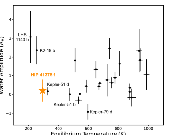
Figure 3: Equilibrium temperature versus 1.4 $\mu$m H₂O feature amplitude ($\rm A_{H}$) for the cooler ($\rm T_{eq}<$ 1000 K) planets sample from Dymont et al. 2021 (points) and HIP 41378 $\rm f$ (orange star). There is no clear trend in $\rm A_{H}$ with planetary temperature.

5.2 Modeling Ring Compositions

We use the WFC3 white light curve to constrain the composition of putative ring particles for HIP 41378 $\rm f$. We infer the ring properties following the framework of Akinsanmi et al. (2020), which found that the observed transit depth of HIP 41378 $\rm f$ could be explained by a ring system extending from $1.05$-$2.59\rm R_{p}$ and inclined by $\sim$25^∘. In this scenario, the underlying planet would have a higher density ($1.2\pm 0.4\,{\rm g}\,{\rm cm}^{-3}$) and a smaller radius ($3.7^{+0.3}_{-0.2}\,R_{\oplus}$), while the ring particles would possess a density of $\rho_{r}=1.08\pm 0.30\,{\rm g}\,{\rm cm}^{-3}$ – lower than expected for rocky materials but comparable to the densities of porous materials comprising some asteroids (Carry, 2012).

Despite the lower signal-to-noise and time sampling of the WFC3 observations, we performed a joint fit to the HST white light curve and K2 (Campaigns 5 and 18) light curves, allowing for different underlying planetary radii in the different bandpasses. Our ringed model fit (constrained mostly by the K2 data) provides a ring density estimate of 1.07$\pm$0.27 g cm^-3, consistent with results in Akinsanmi et al. (2020). The ringed model fit suggests an underlying planetary radius of $3.7^{+0.3}_{-0.2}\,R_{\oplus}$ for the K2 data and $3.9^{+1.2}_{-0.4}\,R_{\oplus}$ for HST.

5.3 Distinguishing Between Rings, Hazes, and High Atmospheric Metallicity

The featureless near-infrared transmission spectrum of HIP 41378 $\rm f$ (Figure 2) might suggest the presence of circumplanetary rings – although high-altitude hazes, a combination of rings and hazes, or a high mean molecular weight atmosphere could also explain the lack of spectral features. Rings composed of large ($>$10 $\mu$m) particles would result in a fairly flat spectrum with weak spectral features in the limit that it dominates over any signal from the planet’s atmosphere (Ohno & Tanaka, 2021; Ohno & Fortney, 2022). In contrast, hazes can flatten spectra fairly easily, as has been observed for other planets (e.g., Kreidberg et al. 2014; Libby-Roberts et al. 2020).

An enticing prospect for breaking the degeneracy between rings, metallicity, and aerosols is to obtain transmission spectra at near- and mid-infrared wavelengths. As shown by Ohno & Tanaka (2021), a super-puff with a hazy atmosphere would be expected to have a strongly sloped transmission spectrum in which the transit depth is much larger at bluer wavelengths than at redder wavelengths. This effect occurs because of the anticipated small size ($<$1 $\mu$m) of lofted dust particles. Conversely, planetary rings are likely composed of significantly larger particles, leading to less variation in transit depth with wavelength.

Using PandExo (Batalha et al., 2017), we simulated JWST observations of a single transit with MIRI LRS ($\sim$5-12 $\mu$m), NIRSpec Prism ($\sim$0.5-5.5 $\mu$m), NIRISS SOSS order 1 ($\sim$0.6-3 $\mu$m), and NIRCam f322 ($\sim$2.4-4 $\mu$m). At a resolution $R=100$, we find that we can measure the transit depth for the high-metallicity clear, hazy, and non-gray rings scenarios to precisions of 85-100 ppm with MIRI, 325-420 ppm with NIRSpec Prism, 230-310 ppm with NIRISS, and 220-280 ppm for NIRCam f322. Observations with MIRI, NIRSpec Prism, NIRISS SOSS, and NIRCam f322 would be able to distinguish between the hazy and clear high-metallicity cases at 3.6-$\sigma$, 5.1-$\sigma$, 4.8-$\sigma$, and 3.4-$\sigma$, between hazy and ringed cases at 5.4-$\sigma$, 6.6-$\sigma$, 6.0-$\sigma$, and 5.1-$\sigma$, or between ringed and clear high-metallicity cases at 1.6-$\sigma$, 1.5-$\sigma$, 1.2-$\sigma$, and 1.7-$\sigma$, respectively. As shown in Figure 2, the models differ in both transit depth and the slope across the near- and mid-infrared. Given the intrinsic challenge of measuring absolute transit depths, the broader wavelength coverage of MIRI and NIRISS SOSS is advantageous because of the increased ability to measure trends in transit depth with wavelength. The ability of JWST to observe continuously for the full transit also provides the opportunity to reveal subtle ring-induced deviations near ingress and egress (Akinsanmi et al., 2020).

5.4 Future Transits

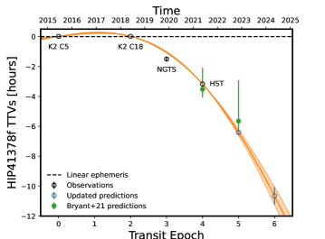
Figure 4: Transit times versus transit epoch for HIP 41378 $\rm f$ for observed transits from previous K2 and NGTS analyses (Vanderburg et al. 2016; Becker et al. 2019; Bryant et al. 2021) compared to the current HST analysis (open black circles). We compare the transit times predicted by Bryant et al. 2021 (green circles) with our new transit predictions based on the HST transit mid-point (open blue circles). The dashed black line marks the linear ephemeris calculated using the period and transit mid-point from Santerne et al. (2019), along with the median TTV signal (orange line) and 1-$\sigma$ uncertainty (shaded region).

To update the prediction of future transits, we reproduced the TTV analysis described in Bryant et al. (2021), based on the Lithwick et al. (2012) formalism on the four epochs observed so far (two K2 epochs, one NGTS, and the HST transit presented in this manuscript). We assumed the timing variations of HIP 41378 $\rm f$ are dominated by the 2:3 resonance with HIP 41378 $\rm e$. As in the aforementioned study, the interaction with the very low-mass HIP 41378 $\rm d$ is expected to be negligible. We used emcee to explore the posterior distribution with 40 walkers of 200,000 steps after a burn-in of 100,000 iterations. Priors were defined following the results of Santerne et al. (2019). We predict that the next transits of HIP 41378 $\rm f$ should occur on $\rm T_{C}$ = BJD 2459897.046 $\pm$ 0.008 (mid-transit on 2022-11-13 at 13:06:28.30 UT) and $\rm T_{C}$ = BJD 2460438.95 $\pm$ 0.02 (mid-transit on 2024-05-08 at 10:47:02.33 UT).

As displayed in Figure 4, the measured transit time is 21 minutes later than the value predicted by Bryant et al. (2021) but is fully compatible with that prediction within 68.3%. We did not detect a transit of HIP 41378 $\rm e$ in our HST data, which is unsurprising given the short duration of our observations compared to the length of the transit window for the planet. Given the long period of HIP 41378 $\rm f$, there are only a few opportunities to observe its transit during JWST’s lifetime. No JWST observations are currently planned for future transits of this target, although these rare events present a unique opportunity to characterize the atmospheric properties of a cool, low mass giant planet.

6 Conclusions

Using HST/WFC3, we observed a transit of the low-mass, long-period temperate giant planet HIP 41378 $\rm f$ to measure its near-infrared transmission spectrum. Based on these measurements, our key results about the atmospheric properties of this planet and opportunities for future observations can be summarized as follows:

• The transmission spectrum is featureless between $1.1-1.7\,\mu{\rm m}$, with no evidence of gaseous molecular features. Based on comparisons to 1D radiative-convective forward models, we rule out clear low metallicity atmospheres, but cannot distinguish between high metallicities, high-altitude hazes, and circumplanetary rings with the current observations.

• In the context of other cooler, low density exoplanets, HIP 41378 $\rm f$’s featureless spectrum suggests that flat spectra are possibly a population property of ultra-low density planets. This planet also complicates the picture of cloudiness versus temperature.

• Future JWST observations (e.g., MIRI, NIRSpec, NIRISS, NIRCam) can distinguish at $>$1-$\sigma$ confidence between the super-puff scenario in which HIP 41378 $\rm f$ is a low-density planet shrouded in a high-altitude aerosol layer, the ringed scenario in which the planet itself is much smaller than expected from the observed optical and near-infrared transit depths, and a clear high mean molecular weight atmosphere scenario.

• We predict the next transits of HIP 41378 $\rm f$ to occur at BJD = 2459897.046 $\pm$ 0.008 and BJD = 2460438.95 $\pm$ 0.02. These upcoming transits provide a rare opportunity to observe the atmospheric properties of a low mass, temperate gas giant planet with JWST, thereby expanding our efforts for comparative exoplanetology.

With the current HST observations, it is also possible to place constraints on the potential presence of exomoons. A $1.5\,\rm R_{\oplus}$ moon would produce a 115 ppm transit (comparable to the precision we achieve in each spectrophotometric channel). Although a lunar transit would cause a noticeable deviation in the light curve, the moon would have to be precisely aligned and at a favorable orbital phase. A moon detection is therefore unlikely, but we will discuss the limits from this serendipitous search in a follow-up paper.

References

- Adams et al. (2019) Adams, D., Gao, P., de Pater, I., & Morley, C. V. 2019, ApJ, 874, 61, doi: 10.3847/1538-4357/ab074c
- Aizawa et al. (2018) Aizawa, M., Masuda, K., Kawahara, H., & Suto, Y. 2018, AJ, 155, 206, doi: 10.3847/1538-3881/aab9a1
- Akinsanmi et al. (2020) Akinsanmi, B., Santos, N. C., Faria, J. P., et al. 2020, A&A, 635, L8, doi: 10.1051/0004-6361/202037618
- Alam et al. (2020) Alam, M. K., López-Morales, M., Nikolov, N., et al. 2020, AJ, 160, 51, doi: 10.3847/1538-3881/ab96cb
- Alam et al. (2021) Alam, M. K., López-Morales, M., MacDonald, R. J., et al. 2021, ApJ, 906, L10, doi: 10.3847/2041-8213/abd18e
- Ambikasaran et al. (2015) Ambikasaran, S., Foreman-Mackey, D., Greengard, L., Hogg, D. W., & O’Neil, M. 2015, IEEE Transactions on Pattern Analysis and Machine Intelligence, 38, 252, doi: 10.1109/TPAMI.2015.2448083
- Barclay et al. (2021) Barclay, T., Kostov, V. B., Colón, K. D., et al. 2021, arXiv e-prints, arXiv:2109.14608. https://arxiv.org/abs/2109.14608
- Batalha et al. (2017) Batalha, N. E., Mandell, A., Pontoppidan, K., et al. 2017, PASP, 129, 064501, doi: 10.1088/1538-3873/aa65b0
- Becker et al. (2019) Becker, J. C., Vanderburg, A., Rodriguez, J. E., et al. 2019, AJ, 157, 19, doi: 10.3847/1538-3881/aaf0a2
- Benneke et al. (2019) Benneke, B., Wong, I., Piaulet, C., et al. 2019, ApJ, 887, L14, doi: 10.3847/2041-8213/ab59dc
- Berardo et al. (2019) Berardo, D., Crossfield, I. J. M., Werner, M., et al. 2019, AJ, 157, 185, doi: 10.3847/1538-3881/ab100c
- Bryant et al. (2021) Bryant, E. M., Bayliss, D., Santerne, A., et al. 2021, MNRAS, 504, L45, doi: 10.1093/mnrasl/slab037
- Canup (2010) Canup, R. M. 2010, Nature, 468, 943, doi: 10.1038/nature09661
- Carry (2012) Carry, B. 2012, Planet. Space Sci., 73, 98, doi: 10.1016/j.pss.2012.03.009
- Chachan et al. (2020) Chachan, Y., Jontof-Hutter, D., Knutson, H. A., et al. 2020, AJ, 160, 201, doi: 10.3847/1538-3881/abb23a
- Crossfield & Kreidberg (2017) Crossfield, I. J. M., & Kreidberg, L. 2017, AJ, 154, 261, doi: 10.3847/1538-3881/aa9279
- Cuzzi & Estrada (1998) Cuzzi, J. N., & Estrada, P. R. 1998, Icarus, 132, 1, doi: 10.1006/icar.1997.5863
- De Pater et al. (2018a) De Pater, I., Hamilton, D. P., Showalter, M. R., Throop, H. B., & Burns, J. A. 2018a, The Rings of Jupiter, ed. M. S. Tiscareno & C. D. Murray, 125–134, doi: 10.1017/9781316286791.006
- De Pater et al. (2018b) De Pater, I., Renner, S., Showalter, M. R., & Sicardy, B. 2018b, The Rings of Neptune, ed. M. S. Tiscareno & C. D. Murray, 112–124, doi: 10.1017/9781316286791.005
- Dones (1991) Dones, L. 1991, Icarus, 92, 194, doi: 10.1016/0019-1035(91)90045-U
- Draine (2003) Draine, B. T. 2003, ApJ, 598, 1026, doi: 10.1086/379123
- Dymont et al. (2021) Dymont, A. H., Yu, X., Ohno, K., Zhang, X., & Fortney, J. J. 2021, arXiv e-prints, arXiv:2112.06173. https://arxiv.org/abs/2112.06173
- Edwards et al. (2021) Edwards, B., Changeat, Q., Mori, M., et al. 2021, AJ, 161, 44, doi: 10.3847/1538-3881/abc6a5
- Gao et al. (2018) Gao, P., Marley, M. S., & Ackerman, A. S. 2018, ApJ, 855, 86, doi: 10.3847/1538-4357/aab0a1
- Gao et al. (2017) Gao, P., Marley, M. S., Zahnle, K., Robinson, T. D., & Lewis, N. K. 2017, AJ, 153, 139, doi: 10.3847/1538-3881/aa5fab
- Gao & Zhang (2020) Gao, P., & Zhang, X. 2020, ApJ, 890, 93, doi: 10.3847/1538-4357/ab6a9b
- Gaudi et al. (2003) Gaudi, B. S., Chang, H.-Y., & Han, C. 2003, ApJ, 586, 527, doi: 10.1086/367539
- Gibson (2014) Gibson, N. P. 2014, MNRAS, 445, 3401, doi: 10.1093/mnras/stu1975
- Hedman & Chancia (2021) Hedman, M., & Chancia, R. 2021, \psj, 2, 107, doi: 10.3847/PSJ/abfdb6
- Hedman (2015) Hedman, M. M. 2015, ApJ, 801, L33, doi: 10.1088/2041-8205/801/2/L33
- Heising et al. (2015) Heising, M. Z., Marcy, G. W., & Schlichting, H. E. 2015, ApJ, 814, 81, doi: 10.1088/0004-637X/814/1/81
- Jones et al. (2001) Jones, E., Oliphant, T., Peterson, P., et al. 2001, SciPy: Open source scientific tools for Python. http://www.scipy.org/
- Jontof-Hutter et al. (2014) Jontof-Hutter, D., Lissauer, J. J., Rowe, J. F., & Fabrycky, D. C. 2014, ApJ, 785, 15, doi: 10.1088/0004-637X/785/1/15
- Kawashima & Ikoma (2019) Kawashima, Y., & Ikoma, M. 2019, ApJ, 877, 109, doi: 10.3847/1538-4357/ab1b1d
- Kirk et al. (2019) Kirk, J., López-Morales, M., Wheatley, P. J., et al. 2019, AJ, 158, 144, doi: 10.3847/1538-3881/ab397d
- Kirk et al. (2017) Kirk, J., Wheatley, P. J., Louden, T., et al. 2017, MNRAS, 468, 3907, doi: 10.1093/mnras/stx752
- Kirk et al. (2018) —. 2018, MNRAS, 474, 876, doi: 10.1093/mnras/stx2826
- Kirk et al. (2021) Kirk, J., Rackham, B. V., MacDonald, R. J., et al. 2021, AJ, 162, 34, doi: 10.3847/1538-3881/abfcd2
- Kreidberg (2015) Kreidberg, L. 2015, PASP, 127, 1161, doi: 10.1086/683602
- Kreidberg et al. (2014) Kreidberg, L., Bean, J. L., Désert, J.-M., et al. 2014, Nature, 505, 69, doi: 10.1038/nature12888
- Lavvas & Koskinen (2017) Lavvas, P., & Koskinen, T. 2017, ApJ, 847, 32, doi: 10.3847/1538-4357/aa88ce
- Lee & Chiang (2016) Lee, E. J., & Chiang, E. 2016, ApJ, 817, 90, doi: 10.3847/0004-637X/817/2/90
- Libby-Roberts et al. (2020) Libby-Roberts, J. E., Berta-Thompson, Z. K., Désert, J.-M., et al. 2020, AJ, 159, 57, doi: 10.3847/1538-3881/ab5d36
- Lithwick et al. (2012) Lithwick, Y., Xie, J., & Wu, Y. 2012, ApJ, 761, 122, doi: 10.1088/0004-637X/761/2/122
- Lopez & Fortney (2014) Lopez, E. D., & Fortney, J. J. 2014, ApJ, 792, 1, doi: 10.1088/0004-637X/792/1/1
- Magic et al. (2015) Magic, Z., Chiavassa, A., Collet, R., & Asplund, M. 2015, A&A, 573, A90, doi: 10.1051/0004-6361/201423804
- Mandel & Agol (2002) Mandel, K., & Agol, E. 2002, ApJ, 580, L171, doi: 10.1086/345520
- Masuda (2014) Masuda, K. 2014, ApJ, 783, 53, doi: 10.1088/0004-637X/783/1/53
- McCullough & MacKenty (2012) McCullough, P., & MacKenty, J. 2012, Considerations for using Spatial Scans with WFC3, Space Telescope WFC Instrument Science Report
- Millholland (2019) Millholland, S. 2019, ApJ, 886, 72, doi: 10.3847/1538-4357/ab4c3f
- Nicholson et al. (2005) Nicholson, P. D., French, R. G., Campbell, D. B., et al. 2005, Icarus, 177, 32, doi: 10.1016/j.icarus.2005.03.023
- Nikolov et al. (2014) Nikolov, N., Sing, D. K., Pont, F., et al. 2014, MNRAS, 437, 46, doi: 10.1093/mnras/stt1859
- Ohno & Fortney (2022) Ohno, K., & Fortney, J. J. 2022, arXiv e-prints, arXiv:2201.02794. https://arxiv.org/abs/2201.02794
- Ohno & Tanaka (2021) Ohno, K., & Tanaka, Y. A. 2021, ApJ, 920, 124, doi: 10.3847/1538-4357/ac1516
- Piro & Vissapragada (2020) Piro, A. L., & Vissapragada, S. 2020, AJ, 159, 131, doi: 10.3847/1538-3881/ab7192
- Pollack (1975) Pollack, J. B. 1975, Space Sci. Rev., 18, 3, doi: 10.1007/BF00350197
- Poulet et al. (2003) Poulet, F., Cruikshank, D. P., Cuzzi, J. N., Roush, T. L., & French, R. G. 2003, A&A, 412, 305, doi: 10.1051/0004-6361:20031123
- Pu & Valencia (2017) Pu, B., & Valencia, D. 2017, ApJ, 846, 47, doi: 10.3847/1538-4357/aa826f
- Santerne et al. (2019) Santerne, A., Malavolta, L., Kosiarek, M. R., et al. 2019, arXiv e-prints, arXiv:1911.07355. https://arxiv.org/abs/1911.07355
- Saumon & Marley (2008) Saumon, D., & Marley, M. S. 2008, ApJ, 689, 1327, doi: 10.1086/592734
- Schlichting & Chang (2011) Schlichting, H. E., & Chang, P. 2011, ApJ, 734, 117, doi: 10.1088/0004-637X/734/2/117
- Tiscareno et al. (2013) Tiscareno, M. S., Hedman, M. M., Burns, J. A., & Castillo-Rogez, J. 2013, ApJ, 765, L28, doi: 10.1088/2041-8205/765/2/L28
- Tsiaras et al. (2019) Tsiaras, A., Waldmann, I. P., Tinetti, G., Tennyson, J., & Yurchenko, S. N. 2019, Nature Astronomy, 3, 1086, doi: 10.1038/s41550-019-0878-9
- Vanderburg et al. (2016) Vanderburg, A., Becker, J. C., Kristiansen, M. H., et al. 2016, ApJ, 827, L10, doi: 10.3847/2041-8205/827/1/L10
- Vissapragada et al. (2020) Vissapragada, S., Jontof-Hutter, D., Shporer, A., et al. 2020, AJ, 159, 108, doi: 10.3847/1538-3881/ab65c8
- Wang & Dai (2019) Wang, L., & Dai, F. 2019, ApJ, 873, L1, doi: 10.3847/2041-8213/ab0653
- Yu et al. (2021) Yu, X., He, C., Zhang, X., et al. 2021, Nature Astronomy, 5, 822, doi: 10.1038/s41550-021-01375-3
- Zahnle et al. (2016) Zahnle, K., Marley, M. S., Morley, C. V., & Moses, J. I. 2016, ApJ, 824, 137, doi: 10.3847/0004-637X/824/2/137