An Integral Euler Cycle in Normally Complex Orbifolds and $\mathbb{Z}$-valued Gromov–Witten type invariants

Abstract.

We define an integral Euler cycle for a vector bundle $E$ over an effective orbifold $X$ for which $(E,X)$ is (stably) normally complex. The transversality is achieved by using Fukaya–Ono’s “normally polynomial perturbations” [FO97] and Brett Parker’s generalization [Par13] to “normally complex perturbations.” Two immediate applications in symplectic topology are the definition of integer-valued genus-zero Gromov–Witten type invariants for general compact symplectic manifolds using the global Kuranishi chart constructed by Abouzaid–McLean–Smith [AMS21], and an alternative proof of the cohomological splitting theorem for Hamiltonian fibrations over $S^{2}$ with integer coefficients from [AMS21].

1. Introduction

Let $(X,\omega)$ be a closed symplectic manifold and suppose $J:TX\rightarrow TX$ is an almost complex structure tamed by $\omega$. Given a homology class $A\in H_{2}(X;\mathbb{Z})$ and an integer $g\geq 0$, the moduli space of stable $J$-holomorphic maps of class $A$ and genus $g$ with $n$ marked points $\overline{\mathcal{M}}_{g,n}(X,J,A)$ carries a rational virtual fundamental class $[\overline{\mathcal{M}}_{g,n}(X,J,A)]^{\text{vir}}$ as constructed by Fukaya–Ono [FO99] using the theory of Kuranishi structures, along with other constructions by Li–Tian [LT98], Ruan [Rua99], Hofer–Wysocki–Zehnder [HWZ17], Pardon [Par16], and many others. The Gromov–Witten invariants are defined by pairing $[\overline{\mathcal{M}}_{g,n}(X,J,A)]^{\text{vir}}$ with cohomology classes obtained from pulling back classes in $H^{*}(\overline{\mathcal{M}}_{g,n};\mathbb{Q})$ and $H^{*}(X;\mathbb{Q})$ under the forgetful map and the evaluation maps.

The Gromov–Witten invariants are in general $\mathbb{Q}$-valued because of the presence of non-trivial automorphisms of stable maps, though genus-$0$ Gromov–Witten invariants are $\mathbb{Z}$-valued for semi-positive symplectic manifolds as proved by Ruan–Tian [RT95] and studied extensively in [MS04]. Technically speaking, rational numbers show up due to the use of abstract multi-valued perturbations of the $\overline{\partial}_{J}$-equations as from [FO99, LT98, HWZ17, MW17], or because Poincaré duality type constructions only hold over $\mathbb{Q}$ rather than $\mathbb{Z}$ for orbifolds as used in [Rua99, Par16] (see also [LT98, Remark 4] for a discussion about when the invariants are integers).

Motivated by seeking for $\mathbb{Z}$-valued Gromov–Witten type invariants, this paper explains how to construct integral “Euler classes” for an orbifold complex vector bundle over an orbifold endowed with a “normal complex structure” following a proposal of Fukaya–Ono [FO97] and the subsequent development by Parker [Par13]. Combined with recent advances in algebraic topology [Par19, Par20] and regularization of moduli spaces of $J$-holomorphic maps [AMS21], we can study generalized bordism theories over orbispaces and define $\mathbb{Z}$-valued Gromov–Witten type invariants for general symplectic manifolds.

1.1. Statement of main results

Recall that an orbifold is called effective if the local uniformizer group from any orbifold chart acts faithfully.

Theorem 1.1.

Suppose $X$ is a compact effective orbifold without boundary endowed with an almost complex structure and let $\mathcal{E}\rightarrow X$ be a complex orbibundle. Denote by $X^{\rm free}\subset X$ the suborbifold consisting of points with trivial isotropy group. Then there exist normally complex (Definition 3.27) smooth sections $s:X\rightarrow\mathcal{E}$ which is strongly transverse (Definition 6.1) such that $s^{-1}(0)\cap X^{\rm free}$ defines a pseudocycle (Definition 5.7). Moreover, given a pair of such sections $s_{1}$ and $s_{2}$, the pseudocycles $s_{1}^{-1}(0)\cap X^{\rm free}$ and $s_{2}^{-1}(0)\cap X^{\rm free}$ are cobordant. Therefore, homology class defined by the cobordism class of the pseudocycle

$$\chi_{\rm free}^{{\rm FOP}}(X,\mathcal{E}):=[s^{-1}(0)\cap X^{\rm free}]\in H_{*}(X;\mathbb{Z}),$$ (1.1)

which we call by the Fukaya–Ono–Parker–Euler class, is an invariant of ${\mathcal{E}}\to X$.

Remark 1.2.

Zinger [Zin08] proved that any (oriented) pseudocycle in a smooth manifold defines an integral homology class and the space of pseudocycles modulo cobordism is natually isomorphic to the integral homology. In Section 5, we show that a pseudocycle in any Thom–Mather stratified space (including any orbifold equipped with the isotropy stratification, see Section 3.2), defines an integral homology class.

Theorem 1.1 is a special case of Theorem 6.3 in Section 6.2, and we comment on how it generalizes Theorem 1.1. Firstly, the existence of (almost) complex structures can be weakened into the existence of normal complex structures. Given $x\in X$, the tangent space $T_{x}X=(T_{x}X)^{\text{triv}}\oplus(T_{x}X)^{\text{non}}$ is a representation of the isotropy group $G_{x}$ and a normal complex structure on $X$ is a family of complex structures on the direct sum of nontrivial $G_{x}$ isotypic pieces $(T_{x}X)^{\text{non}}$ satisfying certain compatibility conditions, see Section 3.5. In particular, the Fukaya–Ono–Parker–Euler class could have an odd degree. Secondly, the compactness assumption on $X$ can be dropped as follows. Instead of considering a pair $(X,\mathcal{E})$, we can start with a triple $(X,\mathcal{E},s)$ where $s:X\rightarrow\mathcal{E}$ is a smooth section of an complex orbibundle $\mathcal{E}\rightarrow X$ over an arbitrary effective normally complex orbifold $X$, but the zero locus $s^{-1}(0)$ is required to be compact. Then we can construct strongly transverse normally complex perturbations of $s$ “relative to $\infty$” to define an element in $\chi_{\text{free}}^{\text{FOP}}(X,\mathcal{E},s)\in H_{*}(X;\mathbb{Z})$ independent of the perturbation. Thirdly, a strongly transverse normally complex section actually defines an Euler-type class of $\mathcal{E}$ for any given stratum of the isotropy stratification, and the class $\chi_{\text{free}}^{\text{FOP}}(X,\mathcal{E})$ is the one associated to the stratum consisting of points with trivial isotropy group. These classes could be viewed as refinements of the rational orbifold Euler class $\chi^{\rm orb}(X,\mathcal{E})\in H_{*}(X;\mathbb{Q})$ which could be constructed by multi-valued perturbations.

The first main application of Theorem 6.3 concerns about the algebraic topology of bordisms of (derived) orbifolds. To state this result, we introduce the following definition. Note that we do not impose the effectiveness on $D$.

Definition 1.3.

A derived orbifold chart (with boundary) is a triple $(D,E,s)$ where $D$ is a smooth orbifold (with boundary), $E\rightarrow D$ is a smooth orbibundle and $s:D\rightarrow E$ is a smooth section. $(D,E,s)$ is said to be compact if $s^{-1}(0)$ is compact.

Following [Joy07, Par20], we can study geometric bordism type invariants constructed from derived orbifold charts. Let $Y$ be an orbispace, i.e. a topological stack locally modeled on the quotient of a topological space by a finite group (see Definition 7.4), then one can consider compact derived orbifold charts of the form $(D,E,s)$ together with a map $f:D\rightarrow Y$. We introduce an equivalence relation among such quadruples $(D,E,s,f)$ generated by the following relations:

1. (Restriction) $(D,E,s,f)\sim(D^{\prime},E^{\prime},s^{\prime},f^{\prime})$ if $D^{\prime}\subset D$ is an open subset with $s^{-1}(0)\subset D^{\prime}$ and $E^{\prime}=E|_{D^{\prime}}$, $s^{\prime}=s|_{D^{\prime}}$, and $f^{\prime}=f|_{D^{\prime}}$.

2. (Stabilization) $(D,E,s,f)\sim(D^{\prime},E^{\prime},s^{\prime},f^{\prime})$ if $D^{\prime}$ is the total space of a vector bundle $\pi_{F}:F\to D$, $E^{\prime}=\pi_{F}^{*}E\oplus\pi_{F}^{*}F$, $s^{\prime}=\pi_{F}^{*}s\oplus\tau_{F}$ where $\tau_{F}:F\to\pi_{F}^{*}F$ is the tautological section, and $f^{\prime}=f\circ\pi_{F}$.

3. (Cobordism) $(D,E,s,f)\sim(D^{\prime},E^{\prime},s^{\prime},f^{\prime})$ if there is a bordism between them (see Section 7.3).

In fact, we restrict our attention to derived orbifold charts $(D,E,s)$ endowed with a stable complex structure, which is defined to be a stable complex structure on the virtual orbibundle $TD-E$. Then stable complex derived orbifold charts mapped to $Y$ modulo the above equivalence relation defines the stable complex derived orbifold bordism of $Y$, written as $\overline{\Omega}_{*}^{\mathbb{C},\text{der}}(Y)$. This is a generalization of the stable complex bordism group over manifolds. A more detailed and precise exposition is presented in Section 7. In particular, any map $f:M\to Y$ from a closed almost complex manifold $M$ represents an element of $\overline{\Omega}_{*}^{{\mathbb{C}},{\rm der}}(Y)$.

Theorem 1.4.

(= Theorem 7.22) Denote by $\Gamma$ the set of equivalence classes of triples $[G,V,W]$ where $G$ is a finite group and $V,W$ are finite-dimensional complex $G$-representations which do not contain any trivial summand, and where the equivalence is induced from stabilization:

$$(G,V,W)\sim(G,V\oplus R,W\oplus R).$$

For any $[\gamma]\in\Gamma$, there is a well-defined map

$$\mathcal{FOP}_{[\gamma]}:\overline{\Omega}^{\mathbb{C},{\rm der}}_{*}(Y)\rightarrow H_{*-\dim V+\dim W}(Y;\mathbb{Z})$$ (1.2)

which restricts to the pushforward of the usual fundamental class for the trivial $[\gamma]$ and elements represented by maps from compact almost complex manifolds.

We call the set $\Gamma$ from the above theorem the set of stabilized isotropy types. In fact, together with a relative version of the map $\mathcal{FOP}_{[\gamma]}$, we can obtain a natural transformation between two (generalized) homology theories for (orbi)spaces, see Section 7.5. Theorem 1.4 is already nontrivial even when $G$ is the trivial group, as the map $\mathcal{FOP}_{[\gamma]}$ can be used to endow any compact stably complex orbifold which is not necessarily effective an integral “fundamental class”. It is well-known to experts that the set $\overline{\Omega}^{\mathbb{C},\text{der}}_{*}(Y)$ could be very large and complicated. However, we expect that the integral shadow (1.2) is more amenable to manipulate but still contains considerable amount of information.

Our second application of Theorem 6.3 is the construction of $\mathbb{Z}$-valued Gromov–Witten type invariants in symplectic topology as proposed by Fukaya–Ono [FO97]. Besides the transversality issue resolved in proving Theorem 6.3, an accompanying fundamental difficulty in the construction is the lack of smoothness of the moduli space of pseudo-holomorphic curves. One possible approach for a systematic solution to the smoothness problem is to either apply the polyfold theory of Hofer–Wysocki–Zehnder [HWZ07] or the delicate exponential decay estimates of Fukaya–Oh–Ohta–Ono [FOOO16]. Instead, in this paper we appeal to a recent work of Abouzaid–McLean–Smith [AMS21] which ingeniously constructed a global Kuranishi chart with a smoothing on the genus zero Gromov–Witten type moduli space using a geometric perturbation. Using the language of derived orbifold charts, one main result from [AMS21] can be formulated as follows.

Proposition 1.5 ([AMS21, Proposition 5.35, 6.31]).

Let $(X,\omega)$ be a closed symplectic manifold and $J$ be a compatible almost complex structure. Let $A\in H_{2}(X;\mathbb{Z})$ be a homology class and denote by $\overline{\mathcal{M}}_{0,n}(X,J,A)$ the moduli space of genus-$0$ stable $J$-holomorphic maps to $X$ with $n\geq 0$ marked points. Then after choosing certain auxiliary data, there exists a smooth stable complex derived orbifold chart $(D,E,s)$ along with a map

$$\widetilde{\text{st}}\times\widetilde{\text{ev}}:D\rightarrow\overline{\mathcal{M}}_{0,n}\times X^{n}$$

such that the zero locus $s^{-1}(0)$ is isomorphic to $\overline{\mathcal{M}}_{0,n}(X,J,A)$ and the restriction of $\widetilde{\text{st}}\times\widetilde{\text{ev}}$ along $s^{-1}(0)$ coincides with the product of the stabilization map and the evaluation map. Moreover, for different choices of $J$ and auxiliary data, the corresponding derived orbifold charts together with $\widetilde{\text{st}}\times\widetilde{\text{ev}}$ define the same element in $\overline{\Omega}^{\mathbb{C},{\rm der}}_{*}(\overline{\mathcal{M}}_{0,n}\times X^{n})$.

Remark 1.6.

The paper [AMS21] uses the notion of global Kuranishi charts instead of derived orbifold charts. A topological/smooth global Kuranishi chart is a quadruple $(G,D,E,s)$ where $G$ is a compact Lie group, $D$ is a topological/smooth manifold endowed with an almost free continuous/smooth $G$-action, $E$ is a $G$-equivariant vector bundle over $D$, and $s$ is a $G$-equivariant continuous/smooth section of $E\rightarrow D$. The equivalence relations introduced in the definition of $\overline{\Omega}^{\mathbb{C},\text{der}}_{*}$ have counterparts in this context, but there is an additional equivalence relation between global Kuranishi charts, namely identifying $(G,D,E,s)$ with $(G^{\prime}\times G,P,q^{*}E,q^{*}s)$ where $q:P\rightarrow D$ is a $G$-equivariant principal $G^{\prime}$-bundle. This change-of-group operation should be interpreted as choosing different global quotient presentation of the orbifold $[D/G]$, so the arguments in [AMS21] indeed prove the statements in the form of Proposition 1.5.

Theorem 1.7.

Suppose $(X,\omega)$ is a closed symplectic manifold and $A\in H_{2}(X;\mathbb{Z})$. Fix a non-negative integer $n$. Given any $[\gamma]\in\Gamma$ as in Theorem 1.4, there is a well-defined integral homology class

$$[\overline{\mathcal{M}}_{0,n}(X,J,A)]^{\text{vir}}_{[\gamma]}\in H_{*}(\overline{\mathcal{M}}_{0,n}\times X^{n};\mathbb{Z})$$ (1.3)

defined by virtually “counting” $J$-holomorphic maps in $\overline{\mathcal{M}}_{0,n}(X,J,A)$ in the stratum indexed by $[\gamma]$.

Proof.

This is a combination of Theorem 1.4 and Proposition 1.5. ∎

By pairing with classes in $H^{*}(\overline{\mathcal{M}}_{0,n};\mathbb{Z})\otimes_{\mathbb{Z}}H^{*}(X;\mathbb{Z})^{\otimes n}$, we can define $\mathbb{Z}$-valued Gromov–Witten type invariants indexed by the stable isotropy type $\Gamma$. When $(X,\omega)$ is semi-positive and $[\gamma]$ is the trivial stabilized isotropy type, as argued in [LT98, Remark 4], our invariants should match the usual genus zero Gromov–Witten invariants.

Remark 1.8.

As communicated from M. Swaminathan, in the forthcoming work of Hirschi–Swaminathan, following [AMS21], smooth global Kuranishi charts for moduli spaces of $J$-holomorphic map of higher genera will be constructed and such constructions together with stabilization maps and evaluation maps lead to well-defined elements in $\overline{\Omega}^{\mathbb{C},{\rm der}}_{*}(\overline{\mathcal{M}}_{g,n}\times X^{n})$ independent of intermediate auxiliary data. In particular, one could define higher genus integral Gromov–Witten type invariants as in Theorem 1.7. We expect these invariants to satisfy variants of the Kontsevich–Manin axioms and to define versions of cohomological field theories on $H^{*}(X;\mathbb{Z})$.

Another application of our construction is an alternate proof of the main theorem of [AMS21]. This theorem asserts that if $P\rightarrow S^{2}$ is a smooth Hamiltonian fibration over the $2$-sphere with fiber given by a closed symplectic manifold $(X,\omega)$, there is an additive splitting isomorphism

$$H^{*}(P;\mathbb{Z})\cong H^{*}(X;\mathbb{Z})\otimes_{\mathbb{Z}}H^{*}(S^{2};\mathbb{Z}).$$ (1.4)

Via using the virtual class indexed by the trivial group, we provide a simple proof of the isomorphism (1.4) in Section 2 without using Morava K-theories or Atiyah duality for orbifolds. We remark that [AMS21] shows that the splitting (1.4) actually holds for any complex oriented generalized cohomology theory but our proof only works over $\mathbb{Z}$.

1.2. A brief discussion of the proof

Our results have their roots in a brilliant proposal of Fukaya–Ono [FO97]. We explain Fukaya–Ono’s idea in technical terms and discuss how to realize their proposal using extra technical inputs.

We consider the following simplified situation. Suppose the moduli space is contained in a single Kuranishi chart $(G,U,E,S)$ where $G$ is a finite group, $U$ is a smooth $G$-manifold, $E$ (the obstruction space) is a finite-dimensional $G$-representation, and $S:U\to E$ (the Kuranishi map) is a $G$-equivariant smooth map. Then the moduli space is $S^{-1}(0)/G$. Let $U^{G}\subset U$ be the set of $G$-fixed points. We further assume that the normal bundle to $U^{G}$ is trivial with fibre being a $G$-representation $V$ and $U=U^{G}\times V$. We also assume that the obstruction space $E$ does not have a trivial $G$-representation as a summand.

Under these assumptions, the map $S:U\to E$ can be identified with a map with target in the space of smooth $G$-equivariant maps between $V$ and $E$

$$f:U^{G}\rightarrow C^{\infty}(V,E)^{G},$$ (1.5)

where for each $p\in M$, $f(p)$ is the restriction of $S$ to the fiber $\{p\}\times V$. For any such map $f$, we denote the associated Kuranishi map by $S_{f}$, i.e.

$$S_{f}(p,v)=f(p)(v)\in E,\ \forall(p,v)\in U^{G}\times V.$$ (1.6)

We wish to define a (relative) homology class of expected degree ${\rm dim}U^{G}+{\rm dim}V-{\rm dim}E$ represented by $S_{f}^{-1}(0)/G$ for a transverse section $S_{f}$. In general, due to the failure of equivariant transversality, such a transverse section does not exist. Indeed $S_{f}$ necessarily vanishes along $M$ whose dimension could be much higher than the expected dimension.

Fukaya–Ono proposed a solution by considering normally complex polynomial perturbations. Assume that both $V$ and $E$ are complex $G$-representations. In applications, such complex structures comes from the nature of the Cauchy–Riemann operator. Then under the correspondence in (1.5) and (1.6) we consider perturbations of $S_{P}$ corresponding to maps of the form

$$P:U^{G}\rightarrow{\rm Poly}_{d}^{G}(V,E)$$

where ${\rm Poly}_{d}^{G}(V,E)\subset C^{\infty}(V,E)^{G}$ is the space of $G$-equivariant complex polynomial maps of degree at most $d$. When $d$ is large enough, Fukaya–Ono showed in [FO97] that for a generic choice of an element $P\in\text{Maps}(U^{G},{\rm Poly}_{d}^{G}(V,E))$ the zero locus along the stratum with trivial isotropy group under the $G$-action

$${\mathcal{M}}_{P}^{\rm free}:=s_{P}^{-1}(0)\cap(U^{G}\times V^{\text{free}})/G$$ (1.7)

is a smooth manifold of the expected dimension. Most crucially, because $V$ and $E$ are both complex, the set-theoretic boundary of ${\mathcal{M}}_{P}^{\rm free}$ has codimension at least $2$. Therefore, using the notion of pseudocycles or any other essentially equivalent language, an integral homology class can be defined.

However, the right notion of transversality is not only that the free part (1.7) is cut out transversely, but also that its boundary (strata) are cut out transversely. Two technical difficulties arise then. First, although the interior transversality behaves well when we increase the cut-off degree $d$, it was not clear if one has a proper notion of boundary transversality which also behaves well with respect to the change of degrees. More seriously, when the action of $G$ on $V$ has additional orbit types, the pointwise transversality condition depends crucially on the stabilizers. It was not clear if the transversality at one point implies the transversality at nearby points with smaller stabilizers. More precisely, for any nontrivial subgroup $H<G$, let $V_{H}\subset V$ be the space of $H$-fixed points and $N_{H}\subset V$ the complement of $V_{H}$; write $v\in V$ as $(v^{\prime},v^{\prime\prime})$. Then a map $P:U^{G}\to{\rm Poly}_{d}^{G}(V,E)$ induces another normally polynomial section

$$P_{H}:U^{G}\times V_{H}\to{\rm Poly}_{d}^{H}(N_{H},E),\ \ P_{H}(p,v^{\prime}):=P(p)(v^{\prime},\cdot).$$

One thus needs a good notion of boundary transversality which behaves well with respect to the change of groups, i.e., $P$ is transverse implies $P_{H}$ is transverse (or vice versa). Otherwise we will not have the openness of the transversality condition, which could cause serious difficulties to construct global perturbations.

The technical core of our construction is the resolution of the above issues by defining the right notion of boundary transversality using the language of Whitney stratifications. Indeed, the transversality notion for normally polynomial sections is related to the complex affine variety

$$Z_{d}^{G}(V,E):=\{(v,P)\in V\times{\rm Poly}_{d}^{G}(V,E)\ |\ P(v)=0\}$$

and how one decomposes it into strata of manifolds. Specifically, in this paper we define a canonical Whitney stratification on $Z_{d}^{G}(V,E)$ which is a decomposition into algebraic submanifolds that respects the natural action stratification of $V$:

$$V=\bigsqcup_{H<G}V_{H}^{*},\ {\rm where}\ V_{H}^{*}:=\{v\in V\ |\ {\rm the\ stabilizer\ of\ }v\ {\rm is\ }H\}.$$

A map $P:U^{G}\to{\rm Poly}_{d}^{G}(V,E)$ (and its associated Kuranishi map $S_{P}$) is said to be strongly transverse (cf. Definition 6.1) if it is transverse to the image of all strata of $Z_{d}^{G}(V,E)$ under the map $Z_{d}^{G}(V,E)\to{\rm Poly}_{d}^{G}(V,E)$. This Whitney stratification is rather robust so that it transforms naturally with respect to the natural inclusion map

$$Z_{d}^{G}(V,E)\rightarrow Z_{d+d^{\prime}}^{G}(V,E)$$ (1.8)

related to the change of degree (see Theorem 4.12) and the natural restriction map

$$Z_{d}^{G}(V,E)\to V_{H}^{*}\times Z_{d}^{H}(N_{H},E)$$ (1.9)

related to the change of groups (see Theorem 4.18). In this way, the notion of strong transversality of normally polynomial sections is intrinsic. The existence of globally defined strongly transverse normal polynomial perturbations and the relevant cobordism invariance results thus follow by the technical arguments in Section 6. Therefore, the integral cycles and invariants expected by Fukaya–Ono [FO97] can be defined. Note that the use of the canonical Whitney stratification allows us to speak of transversality along each stratum of the isotropy stratification of the ambient orbifold. As a result, we actually obtain a system of integral homology classes indexed by isotropy types.

Remark 1.9.

As mentioned in the course of the proof, there are several crucial points inspired by the unpublished work of Parker [Par13]. Unlike our approach, Parker tried to achieve transversality using a less canonical notion of nice Whitney stratifications on the variety $Z_{d}^{G}(V,E)$. Unfortunately, it is unclear to us how to remove the dependence on the choice of these auxiliary Whitney stratifications. The canonical Whitney stratification on $Z_{d}^{G}(V,E)$ we define in this paper is intrinsic to $Z_{d}^{G}(V,E)$ as it is the “minimal” Whitney stratification respecting the action stratification, and it has better functorial properties.

Remark 1.10.

Parker also introduced the notion of normally complex sections in [Par13] which generalizes normally polynomial sections as from [FO97]. Although normally polynomial sections suffice our needs as demonstrated in Lemma 6.5, working with normally complex sections can provide extra flexibility at various points. Hence we work with normally complex sections throughout the paper and call them the Fukaya–Ono–Parker (FOP for short) sections (Definition 3.25).

Note that showing the existence of strongly transverse sections requires us to work with normally complex effective orbifolds and normally complex orbibundles. To establish Theorem 1.4 and its corollary Theorem 1.7, we make use of the flexibility provided by the stabilization equivalences combined with the “enough vector bundle” theorem proved by Pardon [Par19, Theorem 1.1] to identify a stable complex derived orbifold chart with an effective derived orbifold chart such that the ambient orbifold is almost complex and the orbibundle is complex.

1.3. Relations with other work

1.3.1. $\mathbb{Z}$-valued enumerative invariants in symplectic topology

There are other known $\mathbb{Z}$-valued Gromov–Witten type invariants in symplectic topology. Firstly, as mentioned above, for semi-positive symplectic manifolds, Ruan–Tian’s construction ([RT95]) shows that the genus-$0$ Gromov–Witten invariants are indeed $\mathbb{Z}$-valued. Secondly, there are the celebrated $\mathbb{Z}$-valued Gopakumar–Vafa invariants of Calabi–Yau $3$-folds [GV98a, GV98b] which govern the $\mathbb{Q}$-valued Gromov–Witten invariants as demonstrated in full generality by Ionel–Parker [IP18]. It was speculated by some experts (e.g. [Joy07, Section 6.3]) that the invariants defined using Fukaya–Ono’s normally polynomial sections are related to the Gopakumar–Vafa invariants. However, recent developments [DW19], [BS21], which should be viewed as continuations of the groundbreaking work of Taubes in dimension $4$ [Tau96], construct $\mathbb{Z}$-valued invariants of Calabi–Yau $3$-folds by (virtually) counting embedded pseudo-holomorphic curves and these invariants seems to be better connected with the Gopakumar–Vafa invariants. Lastly, the $K$-theoretic Gromov–Witten invariants, defined by Givental and Lee [Lee04] for algebraic objects (which are expected to exist for general symplectic manifolds in light of [AMS21, Section 6.12]), are also $\mathbb{Z}$-valued.

1.3.2. Topological construction and the Floer-theoretic counterpart

Recall that the typical method of defining the (${\mathbb{Q}}$-valued) traditional Gromov–Witten invariants goes through the inductive construction of transverse multisections on a Kuranishi atlas (good coordinate system) over a moduli space. As one only needs transversality in the topological sense, smoothness of coordinate changes are not necessary for the construction (see [LT98] and the case of gauged linear sigma model in [TX18, TX21]). It is expected that one can use normally polynomial sections to define Floer homology with ${\mathbb{Z}}$ or ${\mathbb{Z}}_{2}$-coefficients. A relevant work along this line is [FOOO13] which uses the notion of “normally conical perturbations” to define Lagrangian Floer homology for spherically positive symplectic manifolds. We believe that our integral Euler classes are topological invariants, but to carry out the constructions we need to use topological transversality and the theory of micro-bundles. Working out all the arguments in the topological category would ease up the technical difficulties in deriving Floer-theoretic applications including the weak Arnol’d conjecture over $\mathbb{Z}$, which improves the main result from [AB21].

1.3.3. $\mathbb{Z}$-valued invariants in algebraic geometry

There are several types of enumerative invariants constructed using algebraic geometry, most notably the Donaldson–Thomas invariants [Tho00] and the Pandharipande–Thomas invariants [PT09]. Although these invariants are closely tied with the Gromov–Witten invariants [MNOP06a, MNOP06b], their constructions depend on sheaf theory. Fukaya–Ono’s proposal is differential-topological in nature, as it is still a variant of the general position argument. It would be interesting to see if the virtual classes $[\overline{\mathcal{M}}_{0,n}(X,J,A)]^{\text{vir}}_{[\gamma]}$ admit a purely algebro-geometric interpretation. As remarked before, the classes $[\overline{\mathcal{M}}_{0,n}(X,J,A)]^{\text{vir}}_{[\gamma]}$ are refinements of the traditional rational virtual class $[\overline{\mathcal{M}}_{0,n}(X,J,A)]^{\text{vir}}$, thus an algebro-geometric construction of them might shed light on refinements of other curve-counting invariants.

1.3.4. Wasserman’s theorem and stable homotopy theory

A renowned theorem of Wasserman [Was69], recaptured in [Par20, Theorem 5.6], provides a sufficient condition for equivariant transversality to hold. Our result can be interpreted as a variant of Wasserman’s theorem given the presence of normal complex structures, whose existence allows us to extract more regularity. Rather than developing a theory of stable normal complex bordisms, we confine ourselves with stable complex bordisms of derived orbifolds because the Pontryagin–Thom construction which identifies geometric bordisms with homotopical cobordisms holds in this case [Par20, Theorem 1.4]. The homotopical cobordism perspective gives far-reaching corollaries of Wasserman’s theorem, see [Sch18, Theorem 6.2.33]. As mentioned by [Par20, Remark 5.7], it is an interesting question to understand Fukaya–Ono’s proposal on the homotopical cobordism side.

1.4. Plan of the paper

We start with a new proof of Abouzaid–McLean–Smith’s cohomological splitting theorem over $\mathbb{Z}$ in Section 2 to demonstrate the utility of our construction. Then we introduce basic notions related to orbifolds in Section 3, especially the notion of normal complex structure (Definition 3.22) and FOP section (Definition 3.27). In Section 4, we study the canonical Whitney stratification on the universal zero locus $Z_{d}^{G}(V,W)$ and understand its behavior under the change of degrees and groups. Section 5 proves that any pseudocycle in a Thom–Mather stratified space defines an integral homology class. The main theorem is established in Section 6. In Section 7, we discuss how to use FOP perturbations to study stable complex derived bordisms over orbispaces. Finally, the necessacry background and results on Whitney stratifications are discussed in Appendix A.

Remark 1.11.

When defining the ${\mathbb{Z}}$-valued genus zero curve counting invariants, or equivalently the homology class (1.3), as $\overline{\mathcal{M}}_{0,n}$ is a manifold, we do not need the general result about pseudocycles in Thom–Mather stratified spaces. We also do not need to the more general algebraic topology result Theorem 1.4. Hence results in Section 5 and Section 7 can be bypassed.

1.5. Acknowledgements

We would like to thank Mohammed Abouzaid, Kenji Fukaya, Helmut Hofer, John Pardon, Paul Seidel, Mohan Swaminathan, and Dingyu Yang for useful correspondences and discussions at various stages of this project. The first-named author would like to thank his advisor John Pardon for constant encouragement and support. The second-named author would like to thank his family for their love and support during the Covid-19 pandemic.

2. A simple proof of Abouzaid–McLean–Smith’s splitting theorem

Let $(X,\omega)$ be a closed symplectic manifold. Denote by ${\rm Ham}(X,\omega)$ the group of Hamiltonian diffeomorphisms of $X$. Given an element $\phi\in\pi_{1}{(\rm Ham}(X,\omega))$, one can construct a fibration $P_{\phi}\rightarrow S^{2}$ with fiber symplectomorphic to $X$ and structure group ${\rm Ham}(X,\omega)$ from the clutching construction using $\phi$. We use Theorem 6.3 to give an alternative proof of [AMS21, Theorem 1.1]:

Theorem 2.1.

There is an additive splitting $H^{*}(P_{\phi};\mathbb{Z})\cong H^{*}(X;\mathbb{Z})\otimes_{\mathbb{Z}}H^{*}(S^{2};\mathbb{Z})$.

Denote by $res:H^{*}(P_{\phi};\mathbb{Z})\rightarrow H^{*}(X;\mathbb{Z})$ the restriction map induced by the inclusion of a fiber $X\hookrightarrow P_{\phi}$. The proof is based on constructing a map $s_{\phi}:H^{*}(X;\mathbb{Z})\rightarrow H^{*}(P_{\phi};\mathbb{Z})$ such that the composition $res\circ s_{\phi}$ is the identity map on $H^{*}(X;\mathbb{Z})$. Following [AMS21, Section 3], we introduce the following auxiliary spaces. Let $\mathbb{S}$ be the one-point blow-up of $\mathbb{CP}^{1}\times\mathbb{CP}^{1}$. The composition of the blow-down map and the projection to the second factor defines a map $\pi_{B}:\mathbb{S}\rightarrow B=\mathbb{CP}^{1}$ which is a $\mathbb{CP}^{1}$ fibration with one reducible fiber over $0\in B$. For each $t\in B$, write $\mathbb{S}_{t}:=\pi_{B}^{-1}(t)$. Then there exists a symplectic fibration $\pi_{\mathbb{S}}:\tilde{P}\rightarrow\mathbb{S}$ such that:

1. over a neighborhood $W_{\infty}$ of $\infty\in B$, the space $\tilde{P}$ is isomorphic to the trivial symplectic fibration $(S^{2}\times W_{\infty}\times X,\omega_{S^{2}}\oplus\omega_{S^{2}}|_{W_{\infty}}\oplus\omega)$ and the projection $\pi_{B}:\pi_{B}^{-1}(W_{\infty})\rightarrow W_{\infty}$ coincides with the natural projection $S^{2}\times W_{\infty}\rightarrow W_{\infty}$;

2. the preimage of the reducible fiber $\mathbb{S}_{0}\cong\mathbb{CP}^{1}\vee\mathbb{CP}^{1}$ under $\pi_{\mathbb{S}}$ is given by $P_{\phi}\cup_{X}P_{\phi^{-1}}$ such that each component carries the canonical deformation class of the symplectic structure. Denote $\mathbb{S}_{0}=\mathbb{S}_{\phi}\vee\mathbb{S}_{\phi^{-1}}$ where $\mathbb{S}_{\phi}$ resp. $\mathbb{S}_{\phi^{-1}}$ is the base of $P_{\phi}$ resp. $P_{\phi^{-1}}$.

Denote by $S^{2}_{hor}$ the image of a holomorphic section of $\pi_{B}:\mathbb{S}\rightarrow B=\mathbb{CP}^{1}$ which passes through $\mathbb{S}_{\phi}\setminus\mathbb{S}_{\phi^{-1}}$. Let $(S^{2}\times X)_{hor}$ be the preimage of $S^{2}_{hor}$ under $\pi_{\mathbb{S}}$. Then $(S^{2}\times X)_{hor}$ is symplectically deformation equivalent to the product $(S^{2}\times X,\omega_{S^{2}}\oplus\omega)$. Define $X_{t}$ to be the the fiber of the projection $\pi_{\mathbb{S}}|_{(S^{2}\times X)_{hor}}:(S^{2}\times X)_{hor}\rightarrow S^{2}_{hor}$ over $t\in S^{2}_{hor}$. Denote by $P_{t}$ the space $\tilde{P}|_{\mathbb{S}_{t}}$ for $t\neq 0$. See Figure 1 for illustration.

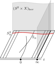
Figure 1. The fibration $\tilde{P}$.

We choose a compatible almost complex structure $J$ on $\tilde{P}$ making the projection $\pi_{\mathbb{S}}:\tilde{P}\rightarrow\mathbb{S}$ pseudo-holomorphic. Moreover, we require that over $S^{2}\times W_{\infty}\times X$, the almost complex structure $J$ is the direct sum of a compatible almost complex structure on $X$ and the standard integrable complex structures on the $S^{2}$ factors. Let $A\in H_{2}(\tilde{P};\mathbb{Z})$ be the homology class represented by $S^{2}\times\{\infty\}\times\{pt\}\subset S^{2}\times W_{\infty}\times X$. We consider the moduli space $\overline{\mathcal{M}}_{0,2}(X,J,A)$ with the evaluation map $ev:\overline{\mathcal{M}}_{0,2}(X,J,A)\rightarrow\tilde{P}\times\tilde{P}$. Define

$$\overline{\mathcal{M}}_{h}:=ev^{-1}(\tilde{P}\times(S^{2}\times X)_{hor})$$

and its subspaces $\overline{\mathcal{M}}_{\infty}:=ev^{-1}(P_{\infty}\times(S^{2}\times X)_{hor})$ and $\overline{\mathcal{M}}_{\phi}:=ev^{-1}(P_{\phi}\times(S^{2}\times X)_{hor})$. After applying the evaluation map, we can view $\overline{\mathcal{M}}_{\phi}$ as a correspondence

(2.1)

Then given any homology class $\alpha\in H_{*}(\overline{\mathcal{M}}_{\phi};\mathbb{Z})$, we can define a homomorphism

$$\Phi_{\alpha}:H^{*}(S^{2}\times X;\mathbb{Z})\rightarrow H^{*}(P_{\phi};\mathbb{Z})$$ (2.2)

by the composition

$$H^{*}((S^{2}\times X)_{hor};\mathbb{Z})\xrightarrow{\pi_{hor}^{*}}H^{*}(\overline{\mathcal{M}}_{\phi};\mathbb{Z})\xrightarrow{\cap\alpha}H_{*}(\overline{\mathcal{M}}_{\phi};\mathbb{Z})\xrightarrow{(\pi_{\phi})_{*}}H_{*}(P_{\phi};\mathbb{Z})\xrightarrow{{\rm PD}}H^{*}(P_{\phi};\mathbb{Z}),$$

where ${\rm PD}$ is the Poincaré duality isomorphism. The map $s_{\phi}:H^{*}(X;\mathbb{Z})\rightarrow H^{*}(P_{\phi};\mathbb{Z})$ leading to a proof of Theorem 2.1 is constructed by composing certain $\Phi_{\alpha}$ with the map $pr^{*}:H^{*}(X;\mathbb{Z})\rightarrow H^{*}(S^{2}\times X;\mathbb{Z})$ induced by the projection $pr:S^{2}\times X\rightarrow X$. To be more precise, such a class $\alpha$ is produced using the FOP perturbation and it actually lies inside a thickening of the moduli space $\overline{\mathcal{M}}_{\phi}$.

Lemma 2.2.

There exists a smooth stable complex compact effective derived orbifold chart $(D,E,s)$ such that there exists an isomorphism $s^{-1}(0)\cong\overline{\mathcal{M}}_{0,2}(X,J,A)$. Moreover, the evaluation maps $ev_{i}:\overline{\mathcal{M}}_{0,2}(X,J,A)\rightarrow\tilde{P}$ for $i=1,2$ extend to

which are smooth submersions.

Proof.

This is a reformulation of the results from [AMS21, Section 5.8]. The construction of stable complex structure is standard in Gromov–Witten theory. ∎

Lemma 2.3.

Define $D_{\infty}$ by the fiber square

$$\vbox{ \lx@xy@svg{\hbox{\raise 0.0pt\hbox{\kern 37.19374pt\hbox{\ignorespaces\ignorespaces\ignorespaces\hbox{\vtop{\kern 0.0pt\offinterlineskip\halign{\entry@#!@&&\entry@@#!@\cr&&\\&&\crcr}}}\ignorespaces{\hbox{\kern-10.07848pt\raise 0.0pt\hbox{\hbox{\kern 0.0pt\raise 0.0pt\hbox{\hbox{\kern 3.0pt\raise 0.0pt\hbox{$\textstyle{D_{\infty}\ignorespaces\ignorespaces\ignorespaces\ignorespaces\ignorespaces\ignorespaces\ignorespaces\ignorespaces}$}}}}}}}\ignorespaces\ignorespaces\ignorespaces\ignorespaces{}{\hbox{\lx@xy@droprule}}\ignorespaces{\hbox{\kern 0.0pt\raise-27.95055pt\hbox{\hbox{\kern 0.0pt\raise 0.0pt\hbox{\lx@xy@tip{1}\lx@xy@tip{-1}}}}}}{\hbox{\lx@xy@droprule}}{\hbox{\lx@xy@droprule}}\ignorespaces\ignorespaces\ignorespaces\ignorespaces{}{\hbox{\lx@xy@droprule}}\ignorespaces{\hbox{\kern 96.35974pt\raise 0.0pt\hbox{\hbox{\kern 0.0pt\raise 0.0pt\hbox{\lx@xy@tip{1}\lx@xy@tip{-1}}}}}}{\hbox{\lx@xy@droprule}}{\hbox{\lx@xy@droprule}}{\hbox{\kern 61.19374pt\raise 0.0pt\hbox{\hbox{\kern 0.0pt\raise 0.0pt\hbox{\hbox{\kern 3.0pt\raise 0.0pt\hbox{$\textstyle{}$}}}}}}}{\hbox{\kern 96.35974pt\raise 0.0pt\hbox{\hbox{\kern 0.0pt\raise 0.0pt\hbox{\hbox{\kern 3.0pt\raise 0.0pt\hbox{$\textstyle{D\ignorespaces\ignorespaces\ignorespaces\ignorespaces}$}}}}}}}\ignorespaces\ignorespaces\ignorespaces\ignorespaces{}{\hbox{\lx@xy@droprule}}\ignorespaces\ignorespaces\ignorespaces{\hbox{\kern 103.63821pt\raise-19.79414pt\hbox{{}\hbox{\kern 0.0pt\raise 0.0pt\hbox{\hbox{\kern 3.0pt\hbox{\hbox{\kern 0.0pt\raise-2.96667pt\hbox{$\scriptstyle{\tilde{ev}_{1}\times\tilde{ev}_{2}}$}}}\kern 3.0pt}}}}}}\ignorespaces{\hbox{\kern 103.63821pt\raise-29.36607pt\hbox{\hbox{\kern 0.0pt\raise 0.0pt\hbox{\lx@xy@tip{1}\lx@xy@tip{-1}}}}}}{\hbox{\lx@xy@droprule}}{\hbox{\lx@xy@droprule}}{\hbox{\kern-37.19374pt\raise-39.5883pt\hbox{\hbox{\kern 0.0pt\raise 0.0pt\hbox{\hbox{\kern 3.0pt\raise 0.0pt\hbox{$\textstyle{P_{\infty}\times(S^{2}\times X)_{hor}\ignorespaces\ignorespaces\ignorespaces\ignorespaces}$}}}}}}}\ignorespaces\ignorespaces\ignorespaces\ignorespaces{}{\hbox{\lx@xy@droprule}}\ignorespaces\ignorespaces\ignorespaces{\hbox{\kern 47.75761pt\raise-45.01884pt\hbox{{}\hbox{\kern 0.0pt\raise 0.0pt\hbox{\hbox{\kern 3.0pt\hbox{\hbox{\kern 0.0pt\raise-2.43056pt\hbox{$\scriptstyle{{\rm inclusion}}$}}}\kern 3.0pt}}}}}}\ignorespaces{\hbox{\kern 91.19374pt\raise-39.5883pt\hbox{\hbox{\kern 0.0pt\raise 0.0pt\hbox{\lx@xy@tip{1}\lx@xy@tip{-1}}}}}}{\hbox{\lx@xy@droprule}}{\hbox{\lx@xy@droprule}}{\hbox{\kern 61.19374pt\raise-39.5883pt\hbox{\hbox{\kern 0.0pt\raise 0.0pt\hbox{\hbox{\kern 3.0pt\raise 0.0pt\hbox{$\textstyle{}$}}}}}}}{\hbox{\kern 91.19374pt\raise-39.5883pt\hbox{\hbox{\kern 0.0pt\raise 0.0pt\hbox{\hbox{\kern 3.0pt\raise 0.0pt\hbox{$\textstyle{\tilde{P}\times\tilde{P}}$}}}}}}}\ignorespaces}}}}\ignorespaces}. \textstyle{D_{\infty}\ignorespaces\ignorespaces\ignorespaces\ignorespaces\ignorespaces\ignorespaces\ignorespaces\ignorespaces} \textstyle{D\ignorespaces\ignorespaces\ignorespaces\ignorespaces} \scriptstyle{\tilde{ev}_{1}\times\tilde{ev}_{2}} \textstyle{P_{\infty}\times(S^{2}\times X)_{hor}\ignorespaces\ignorespaces\ignorespaces\ignorespaces} \scriptstyle{{\rm inclusion}} \textstyle{\tilde{P}\times\tilde{P}} \textstyle{D_{\infty}\ignorespaces\ignorespaces\ignorespaces\ignorespaces\ignorespaces\ignorespaces\ignorespaces\ignorespaces} \textstyle{D\ignorespaces\ignorespaces\ignorespaces\ignorespaces} \scriptstyle{\tilde{ev}_{1}\times\tilde{ev}_{2}} \textstyle{P_{\infty}\times(S^{2}\times X)_{hor}\ignorespaces\ignorespaces\ignorespaces\ignorespaces} \scriptstyle{{\rm inclusion}} \textstyle{\tilde{P}\times\tilde{P}}$$

Then the triple $(D_{\infty},E_{\infty},s_{\infty}):=(D_{\infty},E|_{D_{\infty}},s|_{D_{\infty}})$ is a derived orbifold chart with stable (normal) complex structure such that $s^{-1}_{\infty}(0)\cong\overline{\mathcal{M}}_{\infty}$. Similarly, define $D_{h}$ by the fiber square

$$\vbox{ \lx@xy@svg{\hbox{\raise 0.0pt\hbox{\kern 33.26701pt\hbox{\ignorespaces\ignorespaces\ignorespaces\hbox{\vtop{\kern 0.0pt\offinterlineskip\halign{\entry@#!@&&\entry@@#!@\cr&&\\&&\crcr}}}\ignorespaces{\hbox{\kern-8.89171pt\raise 0.0pt\hbox{\hbox{\kern 0.0pt\raise 0.0pt\hbox{\hbox{\kern 3.0pt\raise 0.0pt\hbox{$\textstyle{D_{h}\ignorespaces\ignorespaces\ignorespaces\ignorespaces\ignorespaces\ignorespaces\ignorespaces\ignorespaces}$}}}}}}}\ignorespaces\ignorespaces\ignorespaces\ignorespaces{}{\hbox{\lx@xy@droprule}}\ignorespaces{\hbox{\kern 0.0pt\raise-28.31999pt\hbox{\hbox{\kern 0.0pt\raise 0.0pt\hbox{\lx@xy@tip{1}\lx@xy@tip{-1}}}}}}{\hbox{\lx@xy@droprule}}{\hbox{\lx@xy@droprule}}\ignorespaces\ignorespaces\ignorespaces\ignorespaces{}{\hbox{\lx@xy@droprule}}\ignorespaces{\hbox{\kern 92.43301pt\raise 0.0pt\hbox{\hbox{\kern 0.0pt\raise 0.0pt\hbox{\lx@xy@tip{1}\lx@xy@tip{-1}}}}}}{\hbox{\lx@xy@droprule}}{\hbox{\lx@xy@droprule}}{\hbox{\kern 57.26701pt\raise 0.0pt\hbox{\hbox{\kern 0.0pt\raise 0.0pt\hbox{\hbox{\kern 3.0pt\raise 0.0pt\hbox{$\textstyle{}$}}}}}}}{\hbox{\kern 92.43301pt\raise 0.0pt\hbox{\hbox{\kern 0.0pt\raise 0.0pt\hbox{\hbox{\kern 3.0pt\raise 0.0pt\hbox{$\textstyle{D\ignorespaces\ignorespaces\ignorespaces\ignorespaces}$}}}}}}}\ignorespaces\ignorespaces\ignorespaces\ignorespaces{}{\hbox{\lx@xy@droprule}}\ignorespaces\ignorespaces\ignorespaces{\hbox{\kern 99.71149pt\raise-19.97887pt\hbox{{}\hbox{\kern 0.0pt\raise 0.0pt\hbox{\hbox{\kern 3.0pt\hbox{\hbox{\kern 0.0pt\raise-2.96667pt\hbox{$\scriptstyle{\tilde{ev}_{1}\times\tilde{ev}_{2}}$}}}\kern 3.0pt}}}}}}\ignorespaces{\hbox{\kern 99.71149pt\raise-29.73552pt\hbox{\hbox{\kern 0.0pt\raise 0.0pt\hbox{\lx@xy@tip{1}\lx@xy@tip{-1}}}}}}{\hbox{\lx@xy@droprule}}{\hbox{\lx@xy@droprule}}{\hbox{\kern-33.26701pt\raise-39.95775pt\hbox{\hbox{\kern 0.0pt\raise 0.0pt\hbox{\hbox{\kern 3.0pt\raise 0.0pt\hbox{$\textstyle{\tilde{P}\times(S^{2}\times X)_{hor}\ignorespaces\ignorespaces\ignorespaces\ignorespaces}$}}}}}}}\ignorespaces\ignorespaces\ignorespaces\ignorespaces{}{\hbox{\lx@xy@droprule}}\ignorespaces\ignorespaces\ignorespaces{\hbox{\kern 43.83089pt\raise-45.38829pt\hbox{{}\hbox{\kern 0.0pt\raise 0.0pt\hbox{\hbox{\kern 3.0pt\hbox{\hbox{\kern 0.0pt\raise-2.43056pt\hbox{$\scriptstyle{{\rm inclusion}}$}}}\kern 3.0pt}}}}}}\ignorespaces{\hbox{\kern 87.26701pt\raise-39.95775pt\hbox{\hbox{\kern 0.0pt\raise 0.0pt\hbox{\lx@xy@tip{1}\lx@xy@tip{-1}}}}}}{\hbox{\lx@xy@droprule}}{\hbox{\lx@xy@droprule}}{\hbox{\kern 57.26701pt\raise-39.95775pt\hbox{\hbox{\kern 0.0pt\raise 0.0pt\hbox{\hbox{\kern 3.0pt\raise 0.0pt\hbox{$\textstyle{}$}}}}}}}{\hbox{\kern 87.26701pt\raise-39.95775pt\hbox{\hbox{\kern 0.0pt\raise 0.0pt\hbox{\hbox{\kern 3.0pt\raise 0.0pt\hbox{$\textstyle{\tilde{P}\times\tilde{P}}$}}}}}}}\ignorespaces}}}}\ignorespaces}. \textstyle{D_{h}\ignorespaces\ignorespaces\ignorespaces\ignorespaces\ignorespaces\ignorespaces\ignorespaces\ignorespaces} \textstyle{D\ignorespaces\ignorespaces\ignorespaces\ignorespaces} \scriptstyle{\tilde{ev}_{1}\times\tilde{ev}_{2}} \textstyle{\tilde{P}\times(S^{2}\times X)_{hor}\ignorespaces\ignorespaces\ignorespaces\ignorespaces} \scriptstyle{{\rm inclusion}} \textstyle{\tilde{P}\times\tilde{P}} \textstyle{D_{h}\ignorespaces\ignorespaces\ignorespaces\ignorespaces\ignorespaces\ignorespaces\ignorespaces\ignorespaces} \textstyle{D\ignorespaces\ignorespaces\ignorespaces\ignorespaces} \scriptstyle{\tilde{ev}_{1}\times\tilde{ev}_{2}} \textstyle{\tilde{P}\times(S^{2}\times X)_{hor}\ignorespaces\ignorespaces\ignorespaces\ignorespaces} \scriptstyle{{\rm inclusion}} \textstyle{\tilde{P}\times\tilde{P}}$$

Then $(D_{h},E_{h},s_{h}):=(D_{h},E|_{D_{h}},s|_{D_{h}})$ is a derived orbifold chart with stable (normal) complex structure such that $s_{h}^{-1}(0)\cong\overline{\mathcal{M}}_{h}$.

Proof.

This follows from [AMS21, Corollary 5.36]. Note that the submersive property of the evaluation maps is used here. ∎

Proof of Theorem 2.1.

Consider the stable (normal) complex derived orbifold chart $(D_{h},E_{h},s_{h})$ constructed above. Using Theorem 6.3 associated to the trivial isotropy type, we can find a homology class $\alpha_{h}\in H_{*}(D_{h};\mathbb{Z})$ by choosing a generic FOP perturbation of the section $s_{h}$. Apply the correspondence construction to the diagram

we obtain a homomorphism $\Psi_{h}:H^{*}(S^{2}\times X;\mathbb{Z})\rightarrow H^{*}({\tilde{P}};\mathbb{Z})$.

Using the inclusion maps $\iota_{\infty}:P_{\infty}\hookrightarrow\tilde{P}$ and $\iota_{\phi}:P_{\phi}\hookrightarrow\tilde{P}$, define $\Psi_{\infty}:=\iota_{\infty}^{*}\circ\Psi_{h}$ and $\Psi_{\phi}:=\iota_{\phi}^{*}\circ\Psi_{h}$. They fit into the following commutative diagram

(2.3)

where the rightmost arrows are induced from the inclusion of a fiber. The split right inverse $s_{\phi}$ of the map $res:H^{*}(P_{\phi};\mathbb{Z})\rightarrow H^{*}(X;\mathbb{Z})$ is defined to be $\Psi_{\phi}\circ pr^{*}$. To prove $res\circ s_{\phi}=id$, it suffices to show that $res\circ\Psi_{\infty}\circ pr^{*}=id$.

Let us look at the moduli space $\overline{\mathcal{M}}_{h}$ geometrically. Recall that over a neighborhood $W_{\infty}$ of $\infty\in B$, the fibration $\pi_{\mathbb{S}}:\tilde{P}\rightarrow\mathbb{S}$ is identified with $W_{\infty}\times S^{2}\times X\rightarrow S^{2}\times W_{\infty}$ and the almost complex structure $J$ splits. Moreover, the degree $A$ of the curves is generated by the $S^{2}$-factor of the product. As a result, one has a homeomorphism

$$\overline{\mathcal{M}}_{W_{\infty}}:=ev_{2}^{-1}(\pi_{\mathbb{S}}^{-1}(W_{\infty}\times S^{2}))\cap\overline{\mathcal{M}}_{h}\cong W_{\infty}\times S^{2}\times X.$$ (2.4)

In particular, this open subset of $\overline{\mathcal{M}}_{h}$ is regular and consists of elements with trivial automorphism groups. Therefore, for the derived orbifold chart $(D_{h},E_{h},s_{h})$ constructed for the moduli space $\overline{\mathcal{M}}_{h}$, the section $s_{h}$ is transverse over $\overline{\mathcal{M}}_{W_{\infty}}$. Notice that $s_{h}$ is also a strongly regular FOP section near $\overline{\mathcal{M}}_{W_{\infty}}$ because of the triviality of the automorphism groups.

Now we prove that $res\circ\Psi_{\infty}\circ pr^{*}=id$. Fix $a\in H^{*}(X)$. Then by the main theorem of [Zin08], the Poincaré dual ${\rm PD}(a)\in H_{*}(X)$ can be represented by a pseudocycle $\iota_{a}:N\to X$. The pullback $\tilde{\iota}:S^{2}\times N\to(S^{2}\times X)_{h}\cong S^{2}\times X$ then represents the Poincaré dual of $pr^{*}a$. We may choose a strongly transverse FOP section $s_{h}^{\prime}:D_{h}\to E_{h}$ such that it agrees with $s_{h}$ near $\overline{\mathcal{M}}_{W_{\infty}}$ and such that the evaluation map $ev_{1}:(s_{h}^{\prime})^{-1}(0)\to(S^{2}\times X)_{h}$ is transverse to $\tilde{\iota}(S^{2}\times N)$ as well as its boundary. Then the class $ev_{1}^{*}(pr^{*}a)\cap\alpha_{h}$ is represented by the pseudocycle $ev_{1}^{*}(\tilde{\iota}(S^{2}\times N))\cap(s_{h}^{\prime})^{-1}(0)$. By our choice of the FOP perturbation $s_{h}^{\prime}$, we see that near $W_{\infty}$, this pseudocycle is identified with $W_{\infty}\times S^{2}\times N$ with respect to the homeomorphism (2.4). Then after pushing forward by the evaluation map $ev_{2}$ and intersecting with the fibre $P_{\infty}\in\tilde{P}$, one can see that the cohomology class $\iota_{\infty}^{*}\Psi_{h}(pr^{*}a)\in H^{*}(P_{\infty})$ is the Poincaré dual to the pseudocycle $S^{2}\times N$ in $P_{\infty}\cong S^{2}\times X$. Then after restricting to a fibre $\{pt\}\times X\subset S^{2}\times X$, the resulting cohomology class is the Poincaré dual of $N$, i.e., $a$ itself. ∎

Remark 2.4.

Following Theorem 1.7, if we denote by $\Lambda_{\mathbb{Z}}$ the universal Novikov ring over $\mathbb{Z}$

$$\{\sum a_{i}T^{\lambda_{i}}|a_{i}\in\mathbb{Z},\lambda_{i}\in\mathbb{R},\lambda_{i}\xrightarrow{i\rightarrow\infty}+\infty\},$$

one can define a quantum product over $QH^{*}_{\mathbb{Z}}(X):=H^{*}(X;\Lambda_{\mathbb{Z}})$ after reducing the $\mathbb{Z}$-grading to $\mathbb{Z}/2$-grading by considering the $3$-pointed virtual fundamental class associated to the trivial isotropy type. Given an element $\phi\in\pi_{1}({\rm Ham}(X,\omega))$, one could construct an invertible element in $QH^{*}_{\mathbb{Z}}(X)$ by counting pseudo-holomorphic sections of $P_{\phi}$, which is the analogue of Seidel’s element in our setting. After proving a suitable gluing theorem, one can prove Theorem 2.1 using Seidel’s representation as in [LMP99].

3. Normally complex orbifolds and bundles

3.1. Orbifolds and orbifold vector bundles

We recall the basic definition of effective orbifolds. We follow the definition of [ALR07, Section 1.1]. Working with effective orbifolds allows us to use orbifold charts exclusively without appealing to the language of groupoids. We remark that for our applications in Section 7, we can drop effectiveness by choosing an effective presentation of any given derived orbifold.

Let $X$ be a Hausdorff and second countable topological space. An $n$-dimensional orbifold chart of $X$ is a triple

$$C=(U,{\mathit{\Gamma}},\psi)$$

where $U\subset{\mathbb{R}}^{n}$ is a nonempty open subset, ${\mathit{\Gamma}}$ is a finite group acting effectively and smoothly on $U$, and $\psi:U\to X$ is a ${\mathit{\Gamma}}$-invariant continuous map such that the induced map

$$\underline{\smash{\psi}}:U/{\mathit{\Gamma}}\to X$$

is a homeomorphism onto an open subset of $X$. If $x\in\psi(U)$ we also say that $x$ is contained in the chart $C$.

A chart embedding from another chart $C^{\prime}=(U^{\prime},{\mathit{\Gamma}}^{\prime},\psi^{\prime})$ to $C$ is a smooth (open) embedding $\iota:U^{\prime}\hookrightarrow U$ such that

$$\psi\circ\iota=\psi^{\prime}.$$

It follows that (see [ALR07, Page 3]) given a chart embedding $\iota$ as above there exists a canonical group injection ${\mathit{\Gamma}}^{\prime}\hookrightarrow{\mathit{\Gamma}}$ such that $\iota$ is equivariant. Therefore we often include the group injection as part of the data of a chart embedding.

As we are in the smooth category, we can always find “linear” charts around any point. An orbifold chart $C=(U,{\mathit{\Gamma}},\psi)$ is called linear if ${\mathit{\Gamma}}$ acts linearly on ${\mathbb{R}}^{n}$ and $U\subset{\mathbb{R}}^{n}$ is an invariant open subset. We say that a linear chart is centered at $x\in X$ if $0\in U$ and $x=\psi(0)$.

We say two charts $C_{i}=(U_{i},{\mathit{\Gamma}}_{i},\psi_{i})$, $i=1,2$ are compatible if for each $p\in\psi_{1}(U_{1})\cap\psi_{2}(U_{2})$, there exists an orbifold chart $C_{p}=(U_{p},{\mathit{\Gamma}}_{p},\psi_{p})$ and chart embeddings into both $C_{1}$ and $C_{2}$.

An orbifold atlas ${\mathcal{A}}=\{C_{i}\ |\ i\in I\}$ on $X$ is a collection of mutually compatible charts $C_{i}$ which cover $X$. We say an atlas ${\mathcal{A}}^{\prime}=\{C_{j}^{\prime}\ |\ j\in J\}$ refines ${\mathcal{A}}$, equivalently, ${\mathcal{A}}^{\prime}$ is a refinement of ${\mathcal{A}}$, if for each $C_{j}^{\prime}$ there exists a chart embedding $C_{j}^{\prime}\hookrightarrow C_{i}$ for some $i\in I$. We say two orbifold atlases are equivalent if they have a common refinement. A topological space $X$ together with an equivalence class of orbifold atlases is called a smooth effective orbifold.

Let $X$ be an effective orbifold. A continuous function $f:X\to{\mathbb{R}}$ is called smooth if its pullback to each chart is a smooth function.

Remark 3.1.

One can see that orbifolds are all locally compact. As we also assume they are Hausdorff and second countable, they are paracompact spaces. Hence for any open cover by charts, there exists a subordinate continuous partition of unity. Moreover, as one can approximate continuous functions by smooth functions on each chart, there always exist a subordinate smooth partition of unity.

Remark 3.2.

We also need the notion of orbifolds with boundary. In that case, the domain of a chart $C=(U,{\mathit{\Gamma}},\psi)$ is allowed to be a smooth manifold with boundary. The ${\mathit{\Gamma}}$-action is required to fixed the boundary $\partial U\subset U$ set-wise; moreover, for each $x\in\partial U$, the stabilizer of $x$ is required to fix $\partial U$ pointwise.

Similarly we can define the notion of orbifold vector bundles. Let $X$ be an orbifold, ${\mathcal{E}}$ be a topological space, and $\pi:{\mathcal{E}}\to X$ be a continuous map. A bundle chart of ${\mathcal{E}}\to X$ consists of an orbifold chart $C=(U,{\mathit{\Gamma}},\psi)$ of $X$, a ${\mathit{\Gamma}}$-equivariant smooth vector bundle $\pi_{C}:E\to U$, and a ${\mathit{\Gamma}}$-invariant continuous map $\hat{\psi}:E\to{\mathcal{E}}$ such that the following diagram commutes:

In notation we will use a quadruple $\hat{C}=(U,{\mathit{\Gamma}},E,\hat{\psi})$ to denote the bundle chart where the map $\psi:U\to X$ is determined by the map $\hat{\psi}:E\to{\mathcal{E}}$. We can similarly define the notions of chart embeddings, compatibility, atlases for bundles. Then an orbifold vector bundle structure over $\pi:\mathcal{E}\rightarrow X$ is defined to be an equivalence class of bundle atlases as before. We spell out the definition of sections of an orbifold vector bundle because of their importance in this paper.

Definition 3.3 (Sections).

Let ${\mathcal{E}}\to X$ be an orbifold vector bundle.

1. Let $\hat{C}_{i}=(U_{i},E_{i},{\mathit{\Gamma}}_{i},\hat{\psi}_{i})$, $i=1,2$ be two bundle charts. We say that a ${\mathit{\Gamma}}_{1}$-equivariant section $s_{1}:U_{1}\to E_{1}$ and a ${\mathit{\Gamma}}_{2}$-equivariant section $s_{2}:U_{2}\to E_{2}$ are compatible if for any bundle chart $\hat{C}_{0}=(U_{0},E_{0},{\mathit{\Gamma}}_{0},\hat{\psi}_{0})$ of $E$ and chart embeddings $\hat{\iota}_{i}:\hat{C}_{0}\hookrightarrow\hat{C}_{i}$, $i=1,2$ there holds

   $$\hat{\iota}_{1}^{-1}\circ s_{1}\circ\iota_{1}=\hat{\iota}_{2}^{-1}\circ s_{2}\circ\iota_{2}$$

   as sections of $E_{0}\to U_{0}$.

2. Suppose $\hat{\mathcal{A}}=\{\hat{C}_{i}=(U_{i},E_{i},{\mathit{\Gamma}}_{i},\hat{\psi}_{i})\ |\ i\in I\}$ is a bundle atlas on ${\mathcal{E}}$. A section of $({\mathcal{E}},\hat{\mathcal{A}})$ is a collection $s=(s_{i})_{i\in I}$ where $s_{i}:U_{i}\to E_{i}$ is a ${\mathit{\Gamma}}_{i}$-equivariant smooth section such that each pair in this collection are compatible.

3. We say two atlases together with sections $(\hat{\mathcal{A}}_{1},s_{1})$ and $(\hat{\mathcal{A}}_{2},s_{2})$ are equivalent if $\hat{\mathcal{A}}_{1}$ and $\hat{\mathcal{A}}_{2}$ are equivalent as orbifold atlases and their local representations are all pairwise compatible.

4. A section of ${\mathcal{E}}$ is an equivalence classes of pairs $(\hat{\mathcal{A}},s)$.

Lemma 3.4.

For each section of ${\mathcal{E}}\to X$ and each bundle atlas $\hat{\mathcal{A}}$, there exists a representative $(\hat{\mathcal{A}},s)$ of the given section.

Proof.

Straightforward. ∎

3.2. The isotropy prestratification

One can see from the definition of effective orbifolds that the isomorphism class of the stabilizer of a point $x$ in an orbifold chart $C=(U,{\mathit{\Gamma}},\psi)$ only depends on the point $\psi(x)\in X$. One can use this isomorphism class to decompose the orbifold. Moreover, we can actually obtain a more refined decomposition by using the information in the normal direction.

Definition 3.5.

Consider triples $(G,V,W)$ where $G$ is a finite group, $V$ and $W$ are finite-dimensional (real) representations of $G$ such that the decompositions of $V$ and $W$ into irreducible representations contain no trivial summands. Two triples $(G,V,W)$ and $(G^{\prime},V^{\prime},W^{\prime})$ are called isomorphic if there is a group isomorphism $\varphi_{G}:G\to G^{\prime}$ and equivariant linear isomorphisms $\varphi_{V}:V\to V^{\prime}$, $\varphi_{W}:W\to W^{\prime}$. An isomorphism class of triples is called an isotropy type, denoted by $\gamma$.

Now consider an effective orbifold $X$ with an orbifold vector bundle ${\mathcal{E}}\to X$. For each $p\in X$, consider a bundle chart $\hat{C}=(U,G,E,\hat{\psi})$ centered at $p$. Let $U^{G}\subset U$ be the $G$-fixed point locus. Then over $U^{G}$ one has the $G$-equivariant decomposition

$$TU|_{U^{G}}\cong TU^{G}\oplus NU^{G}$$

where the first resp. the second summand is the direct sum of trivial resp. nontrivial summands of the splitting of fibers into irreducible $G$-representations. One also has the decomposition

$$E|_{U^{G}}\cong\mathring{E}^{G}\oplus\check{E}^{G}$$

where $\mathring{E}^{G}$ is a trivial $G$-representation and $\check{E}^{G}$ is the direct sum of nontrivial irreducible $G$-representations. Define $\gamma_{p}$ to be the isotropy type represented by the triple $(G,V,W)$ where $V$ is fiber of $NU^{G}\to U^{G}$ and $W$ is the fiber of $\check{E}^{G}|_{U^{G}}$. Then $\gamma_{p}$ is well-defined, independent of the choice of charts.

Lemma 3.6.

For each isotropy type $\gamma$ represented by a triple $(G_{\gamma},V_{\gamma},W_{\gamma})$, define

$$X_{\gamma}^{*}=\{p\in X\ |\ \gamma_{p}=\gamma\}$$

Then $X_{\gamma}^{*}$ is a topological manifold of dimension ${\rm dim}X-{\rm dim}V_{\gamma}$ equipped with a natural smooth structure.

Proof.

By definition, for each $p\in X_{\gamma}^{*}$, there exists a bundle chart $(U,G,E,\hat{\psi})$ centered at $p$ such that $\gamma$ is represented by $(G,V,W)$ where $V$ is the fibre of the normal bundle to $U^{G}\subset U$ and $W$ is the fibre of $\check{E}^{G}$ at $0$. Then $U^{G}$ has dimension equal to ${\rm dim}X-{\rm dim}V$. Moreover, a neighborhood of $p$ in $X_{\gamma}^{*}$ is homeomorphic to $\psi(U^{G})$. Hence $X_{\gamma}^{*}$ is a topological manifold and $\psi^{-1}:X_{\gamma}^{*}\cap\psi(U)\to U^{G}\subset U$ is a local chart. It is easy to verify that the atlas on $X_{\gamma}^{*}$ obtained in this way is a smooth atlas. ∎

By Lemma 3.6, we obtain a decomposition of the orbifold $X$ as a locally finite disjoint union of locally closed subsets

$$X=\bigsqcup_{\gamma}X_{\gamma}^{*}.$$ (3.1)

An argument similar to the proof of Lemma 3.6 shows that the frontier condition is satisfied. Therefore, (3.1) defines a prestratification (see Appendix A) called the isotropy prestratification.

For each isotropy type $\gamma$ represented by $(G_{\gamma},V_{\gamma},W_{\gamma})$, define

$$n_{\gamma}:={\rm dim}X-{\rm rank}{\mathcal{E}}-{\rm dim}V_{\gamma}+{\rm dim}W_{\gamma}\in{\mathbb{Z}}.$$ (3.2)

This is the expected dimension of the intersection of $X_{\gamma}^{*}$ and the zero locus of a single-valued section $s:X\to{\mathcal{E}}$ (see Proposition 6.6).

3.3. Riemannian metric

We need to specify certain auxiliary data to aid our later construction. These data include Riemannian metrics on orbifolds and connections on orbifold vector bundles.

Definition 3.7.

A Riemannian metric on an effective orbifold $X$ is a collection of invariant Riemannian metrics $g_{C}$ on all orbifold charts $C=(U,{\mathit{\Gamma}},\psi)$ such that every chart embedding

$$(U^{\prime},{\mathit{\Gamma}}^{\prime},\psi^{\prime})\hookrightarrow(U,{\mathit{\Gamma}},\psi)$$

is isometric.

One can use the standard way to construct Riemannian metrics on orbifolds using smooth partition of unity on orbifolds (see Remark 3.1).

3.3.1. Bundle metrics

We need some technical discussion on metrics on total spaces of vector bundles. Suppose $(M,g^{TM})$ is a Riemannian manifold. Let $\pi:E\to M$ be a vector bundle equipped with a metric $h^{E}$ and a metric-preserving connection $\nabla^{E}$. On the total space $E$ we define a Riemannian metric $g^{TE}$ as follows. Via the horizontal-vertical decomposition $TE\cong\pi^{*}TM\oplus\pi^{*}E$ induced by the connection $\nabla^{E}$ we define $g^{TE}=\pi^{*}g^{TM}\oplus\pi^{*}h^{E}$. We call $g^{TE}$ the bundle metric induced from $g^{TM}$, $h^{E}$, and $\nabla^{E}$.

Lemma 3.8.

Suppose $E$ is endowed with the bundle metric as above. Then

1. Each fiber $E_{p}\subset E$ is totally geodesic.

2. We identify the normal bundle of the $0$-section $(TM)^{\bot}\to M$ naturally with $E$. Then the connection on $(TM)^{\bot}$ induced from the Levi–Civita connection of $g^{TE}$ coincides with $\nabla^{E}$.

Proof.

(1) As the restriction of $g^{TE}$ to each fiber is Euclidean, geodesics in each fiber are straight line segments. To show that a fiber is totally geodesic, one only needs to show that any (short) straight line segments are also geodesics in the totally space. Fix $x\in M$. Choose a local orthonormal frame $e_{1},\ldots,e_{k}$ of $E$ defined over a neighborhood $U_{x}\subset M$ of $x$. For any $p\in E_{x}$, choose $r>0$ sufficiently small such that for any $q\in B_{r}(p,E_{x})$, the shortest geodesic connecting $p$ and $q$ are contained in $\pi^{-1}(U_{x})$. We also assume that $U_{x}$ supports a local coordinate chart $\varphi=(x^{1},\ldots,x^{m}):U_{x}\to{\mathbb{R}}^{m}$. One only needs to show that the straight line segment between $p$ and any $q\in B_{r}(p,E_{x})$ is the shortest geodesic. Suppose $\gamma:[0,d]\to E$ is the shortest geodesic parametrized by arc length. Let $y^{1},\ldots,y^{k}$ be the bundle coordinates associated to the frame $e_{1},\ldots,e_{k}$ and write

$$\gamma(t)=(x^{1}(t),\ldots,x^{m}(t),y^{1}(t),\ldots,y^{k}(t)).$$

We can decompose $\dot{\gamma}(t)$ orthogonally as

$$\dot{\gamma}(t)=\dot{\gamma}^{H}(t)+\dot{\gamma}^{V}(t)$$

where $\dot{\gamma}^{H}(t)$ resp. $\dot{\gamma}^{V}(t)$ is the horizontal resp. vertical part. Then one has

$$1=|\dot{\gamma}(t)|=\sqrt{|\dot{\gamma}^{H}(t)|^{2}+|\dot{\gamma}^{V}(t)|^{2}}\geq|\dot{\gamma}^{V}(t)|=\sqrt{\dot{y}^{1}(t)^{2}+\cdots+\dot{y}^{k}(t)^{2}}.$$

Hence

$$d\geq\int_{0}^{d}\sqrt{\dot{y}^{1}(t)^{2}+\cdots+\dot{y}^{k}(t)^{2}}dt\geq d_{E_{x}}(p,q).$$

However, as $\gamma$ is the shortest geodesic, the above must be an equality. Hence $\gamma(t)$ is contained in the fiber $E_{x}$ and $\gamma(t)$ is the straight line segment. Hence the fiber is totally geodesic.

(2) Choose local coordinates $(x^{1},\ldots,x^{m},y^{1},\ldots,y^{k})$ on the total space as above where the bundle coordinates $y^{\alpha}$ correspond to the choice of local orthogonal frame $e_{1},\ldots,e_{k}$ of $E$. Suppose

$$\nabla_{\partial_{i}}^{E}e_{\alpha}=\omega_{i,\alpha}^{\beta}e_{\beta}.$$

To show that the induced connection on the normal bundle $(TM)^{\bot}\cong E$ coincides with $\nabla^{E}$, one only needs to verify that

$$\langle\nabla_{i}^{TE}\frac{\partial}{\partial y^{\alpha}},\frac{\partial}{\partial y^{\beta}}\rangle=\omega_{i,\alpha}^{\beta}.$$

Indeed, by the formula for the Levi–Civita connection, one has

$$\begin{split}\langle\nabla_{i}^{TE}\frac{\partial}{\partial y^{\alpha}},\frac{\partial}{\partial y^{\beta}}\rangle=&\ \frac{1}{2}\left(\frac{\partial}{\partial x^{i}}\langle\frac{\partial}{\partial y^{\alpha}},\frac{\partial}{\partial y^{\beta}}\rangle+\frac{\partial}{\partial y^{\alpha}}\langle\frac{\partial}{\partial x^{i}},\frac{\partial}{\partial y^{\beta}}\rangle-\frac{\partial}{\partial y^{\beta}}\langle\frac{\partial}{\partial x^{i}},\frac{\partial}{\partial y^{\alpha}}\rangle\right)\\ =&\ \frac{1}{2}\left(\frac{\partial}{\partial y^{\alpha}}\langle\sum_{\gamma,\delta}\omega_{i,\gamma}^{\delta}y^{\gamma}\frac{\partial}{\partial y^{\delta}},\frac{\partial}{\partial y^{\beta}}\rangle-\frac{\partial}{\partial y^{\beta}}\langle\sum_{\gamma,\delta}\omega_{i,\gamma}^{\delta}y^{\gamma}\frac{\partial}{\partial y^{\delta}},\frac{\partial}{\partial y^{\alpha}}\rangle\right)\\ =&\ \frac{1}{2}\left(\omega_{i,\alpha}^{\beta}-\omega_{i,\beta}^{\alpha}\right)\\ =&\ \omega_{i,\alpha}^{\beta}.\end{split}$$

Therefore $\nabla^{(TM)^{\bot}}$ coincides with $\nabla^{E}$. ∎

We would like to identify tubular neighborhoods of fixed point locus with disk bundles of the normal bundle and equip the tubular neighborhoods with bundle metrics. To globalize such bundle metric construction we need to verify certain properties of bundle metrics related to orthogonal decompositions of vector bundles. Let $(M,g^{TM})$ be a Riemannian manifold and $\pi_{\mathring{E}}:\mathring{E}\to M$, $\pi_{\check{E}}:\check{E}\to M$ be two vector bundles equipped with metrics $h^{\mathring{E}}$, $h^{\check{E}}$ and metric preserving connections $\nabla^{\mathring{E}}$, $\nabla^{\check{E}}$. Denote $E=\mathring{E}\oplus\check{E}$ equipped with the product metric $h^{E}=h^{\mathring{E}}\oplus h^{\check{E}}$ and the product connection $\nabla^{E}=\nabla^{\mathring{E}}\oplus\nabla^{\check{E}}$. Then over the total space of $E$ there is the induced bundle metric $g^{TE}$. On the other hand, the total space of $E$ can also be viewed as the total space of the bundle

$$\pi_{\mathring{E}}^{*}\check{E}\to\mathring{E}.$$

There is hence another bundle metric $g^{T\pi_{\mathring{E}}^{*}\check{E}}$ induced from the base metric $g^{T\mathring{E}}$ on $\mathring{E}$, the fiberwise bundle metric $\pi_{\mathring{E}}^{*}h^{\check{E}}$, and the connection $\pi_{\mathring{E}}^{*}\nabla^{\check{E}}$. We would like to show that $g^{TE}$ and $g^{T\pi_{\mathring{E}}^{*}\check{E}}$ coincide.

Corollary 3.9.

The following items are true.

1. Over $\mathring{E}\subset E$, the direct sum decomposition

   $$TE|_{\mathring{E}}\cong T\mathring{E}\oplus\pi_{\mathring{E}}^{*}\check{E}$$

   is orthogonal with respect to the bundle metric $g^{TE}$. Moreover,

   $$g^{TE}|_{\pi_{\mathring{E}}^{*}\check{E}}=\pi_{\mathring{E}}^{*}h^{\check{E}}.$$

2. The connection on $\pi_{\mathring{E}}^{*}\check{E}$ (viewed as a subbundle of $TE|_{\mathring{E}}$) induced from the Levi–Civita connection of $g^{TE}$ coincides with the pullback $\pi_{\mathring{E}}^{*}\nabla^{\check{E}}$.

3. For $(x,\mathring{v})\in\mathring{E}|_{x}$ and $\check{v}\in\check{E}|_{x}$, viewing the latter as a normal vector in $(T_{(x,\mathring{v})}\mathring{E})^{\bot}$, one has

   $$\exp_{(x,\mathring{v})}(\check{v})=(x,\mathring{v}+\check{v}).$$

4. The bundle metric $g^{TE}$ on $E$ (viewed as the total space of $E\to M$) coincides with the bundle metric $g^{T\pi_{\mathring{E}}^{*}\check{E}}$ on $E$ (viewed as the total space of $\pi_{\mathring{E}}^{*}\check{E}$).

Proof.

(1) is straightforward, following from the definition of the bundle metric. (2) is a consequence of the second item of Lemma 3.8. (3) follows from the first item of Lemma 3.8. (4) is a straightforward check using (1)—(3). ∎

3.3.2. Straightened metrics

Now we consider Riemannian metrics on an orbifold chart. Let $U$ be a smooth manifold acted on by a finite group ${\mathit{\Gamma}}$. Let $g$ be a ${\mathit{\Gamma}}$-invariant Riemannian metric on $U$. Then for each subgroup $G\subseteq{\mathit{\Gamma}}$, the metric induces the following objects.

1. The orthogonal decomposition splitting $TU|_{U^{G}}\cong TU^{G}\oplus NU^{G}$ which agrees with the decomposition into the direct sum of trivial $G$-representations and nontrivial $G$-representations.

2. A metric on the normal bundle $NU^{G}\to U^{G}$. Let $N_{\epsilon}(U^{G})\subset NU^{G}$ be the $\epsilon$-disk bundle.

3. The restriction of the Levi–Civita connection on $NU^{G}$. This connection then induces a splitting of $TNU^{G}$ into horizontal and vertical distributions and hence a Riemannian bundle metric on the total space of $NU^{G}$.

4. The exponential map $N_{\epsilon}(U^{G})\to U$ which pushes forward the metric on the total space of $NU^{G}$ to a metric on a tubular neighborhood of $U^{G}$.

Definition 3.10.

Let $G\subseteq{\mathit{\Gamma}}$ be a subgroup. A ${\mathit{\Gamma}}$-invariant Riemannian metric $\tilde{g}$ on $U$ is called straightened along $NU^{G}$ if within a $G$-invariant neighborhood of $U^{G}\subset U$ the push-forward metric $\tilde{g}^{G}$ coincides with $\tilde{g}$. A ${\mathit{\Gamma}}$-invariant metric $\tilde{g}$ is called straightened if it is straightened along $NU^{G}$ for all subgroups $G\subseteq{\mathit{\Gamma}}$.

Lemma 3.11.

Suppose $\tilde{g}$ is straightened along $NU^{G}$ for some subgroup $G\subseteq{\mathit{\Gamma}}$. Then there is a $G$-invariant neighborhood $V\subset U$ of $U^{G}$ such that for every subgroup $H\subseteq G$, the restriction of $\tilde{g}$ to $V$ is straightened along $NV^{H}$.

Proof.

It is a direct consequence of Corollary 3.9. ∎

Definition 3.12.

A Riemannian metric on an effective orbifold $X$ is called straightened resp. straightened near a subset $Y\subset X$ if its pullback to each chart is straightened resp. if its restriction to an open neighborhood of $Y$ is straightened.

It is easy to see that for a Riemannian metric on an orbifold, being straightened is an intrinsic property independent of the choice of an orbifold chart, therefore the above definition is well-defined. Before we show that straightened metrics exist, we consider the following good property of them.

Definition 3.13.

Suppose $W$ is a finite-dimensional real representation of a finite group $G$. Then $W$ can be decomposed as the direct sum of irreducible representations. We call the decomposition

$$W=\mathring{W}^{G}\oplus\check{W}^{G}$$

where $\mathring{W}^{G}$ is the direct sum of all trivial summands and $\check{W}^{G}$ is the direct sum of all nontrivial summands the basic decomposition of $W$ with respect to $G$.

Lemma 3.14.

Suppose $X$ is equipped with a straightened metric. Then for each orbifold chart $C=(U,{\mathit{\Gamma}},\psi)$ with the pullback metric $g_{C}$, for each pair of subgroups $H<G<{\mathit{\Gamma}}$, for each $x\in U^{G}$ and $v\in N_{\epsilon}U^{G}\cap N_{x}U^{G}$ for $\epsilon$ sufficiently small, the following holds. Using the (orthogonal) basic decomposition with respect to $H$

$$NU^{G}\cong(TU^{H}\cap NU^{G})\oplus NU^{H}|_{U^{G}}$$

we write

$$v=(\mathring{v}_{H},\check{v}_{H}).$$

Moreover, we use the exponential map $\exp:N_{\epsilon}U^{G}\to U$ to identify $\check{v}_{H}\in T_{x}U$ with a vector of $NU^{H}|_{\exp_{x}\mathring{v}_{H}}$ and still denote it by $\check{v}_{H}$. Then one has

$$\exp_{x}v=\exp_{\exp_{x}\mathring{v}_{H}}(\check{v}_{H}).$$

Proof.

As the metric is straightened, locally $U$ is isometric to the total space $NU^{G}$. Then the property follows from Corollary 3.9. ∎

Now we prove the existence of straightened metrics by a prototypical induction argument.

Lemma 3.15.

Let $X$ be an effective orbifold and $Y\subset X$ be a compact subset. Then there exists a Riemannian metric $g$ on $X$ which is straightened near $Y$.

Proof.

We define a filtration

$$X_{0}\subset X_{1}\subset\cdots\subset X_{n}=X$$

where $n={\rm dim}X$ as follows: $p\in X_{d}$ if for any orbifold chart $(U,{\mathit{\Gamma}},\psi)$ and any $x\in U$ with $\psi(x)=p$, the dimension of $U^{{\mathit{\Gamma}}_{x}}$ through $x$ is at most $d$, where ${\mathit{\Gamma}}_{x}\subset{\mathit{\Gamma}}$ is the isotropy group of $x$. Then $X_{d}$ is closed. Let $g$ be an arbitrary Riemannian metric on $X$. We modify $g$ inductively such that the modification $g_{d}$ is straightened near $X_{d}\cap Y$. For $d=0$, $X_{0}$ is discrete. Then for each $p\in X_{0}\cap Y$, define a Riemannian metric $g_{p}$ as follows. Choose a linear orbifold chart $C=(U,{\mathit{\Gamma}},\psi)$ centered at $p$. Let $\tilde{g}$ be the metric on $U$ obtained by pulling back $g$ to the chart $C$. Define a metric $\tilde{g}_{p}$ on $U$ whose restriction to a neighborhood of $0\in U$ is equal to the pushforward of the Euclidean metric on $T_{0}U\cong{\mathbb{R}}^{n}$ (induced from $\tilde{g}$) via the exponential map on $U$ centered at $0$. Then $\tilde{g}_{p}$ induces a Riemannian metric in a neighborhood of $p\in X$. As $\tilde{g}_{p}$ is Euclidean near $0$, it is straightened near $p$. Using cut-off functions one can obtain a metric $g_{0}$ which is straightened near $X_{0}\cap Y$.

Suppose we have obtained a metric $g_{d-1}$ straightened over an open neighborhood $V_{d-1}\supset X_{d-1}\cap Y$ for some $d\geq 1$. Then by the compactness of $Y$, one can find finitely many linear orbifold charts $C_{i}=(U_{i},{\mathit{\Gamma}}_{i},\psi_{i})$ for $i=1,2,\ldots,N$ with $U_{i}$ being a radius $2r_{i}$-ball of ${\mathbb{R}}^{n}$ such that

1. $x_{i}=\psi_{i}(0)\in(X_{d}\setminus X_{d-1})\cap Y$.

2. The union of $F_{i}^{\prime}:=\psi_{i}(U_{i}^{\prime})$ with $U_{i}^{\prime}$ being the radius $r_{i}$ ball in $U_{i}$ covers $(Y\cap X_{d})\setminus V_{d-1}$.

We claim that one can find a metric $g_{d,k}$ on $X$ which is straightened near $Y\cap X_{d}\cap(V_{d-1}\cup F_{1}^{\prime}\cup\cdots F_{k}^{\prime})$. Indeed, suppose we have find $g_{d,k-1}$ for some $k\geq 1$. For the chart $C_{k}$, let $\tilde{g}_{d,k-1}$ be the corresponding ${\mathit{\Gamma}}_{k}$-invariant metric on $U_{k}$. Then we can use the exponential map centered at the origin of $U_{k}$ to pushforward the induced bundle metric on the $\epsilon$-disk bundle $N_{\epsilon}U_{k}^{{\mathit{\Gamma}}_{k}}$ (associated to $\tilde{g}_{d,k-1}$) to a neighborhood of $U_{k}^{{\mathit{\Gamma}}_{k}}$, and use a ${\mathit{\Gamma}}_{k}$-invariant cut-off function to extend it to $U_{k}$. This provides a ${\mathit{\Gamma}}_{k}$-invariant metric $\tilde{g}_{C_{k}}$ on the manifold $U_{k}$. Then $\tilde{g}_{C_{k}}$ is straightened near $U_{k}^{{\mathit{\Gamma}}_{k}}$. Let $g_{C_{k}}$ be the corresponding orbifold metric on the open set $F_{k}=\psi_{k}(U_{k})\subset X$. Now choose a cut-off function $\rho_{k}:X\to[0,1]$ supported in $F_{k}$ such that $\rho_{k}\equiv 1$ near $\overline{F_{k}^{\prime}}$ and $\rho_{k}$ vanishes on $X\setminus F_{k}$. Then define

$$g_{d,k}=(1-\rho_{k})g_{d,k-1}+\rho_{k}g_{C_{k}}$$

which is a new Riemannian metric on $X$. We only need to show that this metric is straightened near any point $p\in Y\cap X_{d}\cap(V_{d-1}\cup F_{1}^{\prime}\cup\cdots\cup F_{k}^{\prime})$. Indeed, if $p\in F_{k}^{\prime}$, then locally $g_{d,k}=g_{C_{k}}$ which is straightened near $p$. If $p\notin F_{k}$, then locally $g_{d,k}=g_{d,k-1}$ which is also straightened near $p$. If $p\in F_{k}\setminus F_{k}^{\prime}$, then $p\in Y\cap X_{d}\cap(V_{d-1}\cup F_{1}^{\prime}\cup\cdots\cup F_{k-1}^{\prime})$. Then near $p$ the metric $g_{d,k-1}$ is already straightened. Let $x\in U_{k}$ be a point such that $\psi_{k}(x)=p$. Then $x\in U_{k}^{{\mathit{\Gamma}}_{k}}$. Then near $x$ the metrics $\tilde{g}_{d,k-1}$ and $\tilde{g}_{C_{k}}$ are identical. Hence $g_{d,k}=g_{d,k-1}$ near $x$ so $g_{d,k}$ is straightened near $x$. Then inductively, one can obtain a metric $g_{d}$ which is straightened near $Y\cap X_{d}$. The induction on $d$ provides a metric with desired property. ∎

From the construction used in the proof one can see the following: for a closed subset $Q\subset X$, if we start with a Riemannian metric $g$ on $X$ which is already straightened near $Y\cap Q$, then one can obtain a metric $g^{\prime}$ which is straightened near $Y$ such that it coincides with $g$ in a neighborhood of $Y\cap Q$. Therefore one can obtain a “relative version” of Lemma 3.15. In particular, one can connect any two straightened metric via a one-parameter family.

Lemma 3.16.

For any pair of Riemannian metrics $g_{0}$ and $g_{1}$ on $X$ which are straightened near $Y$, there exists a straightened Riemannian metric on $X\times[0,1]$ which coincides with $g_{i}+dt^{\otimes 2}$ near $X\times\{i\}$ for $i=0,1$.

Proof.

Define $\tilde{X}=X\times[0,1]$ and $\tilde{Y}=Y\times[0,1]$. Let $t$ be the coordinate on $[0,1]$. Consider an arbitrary Riemannian metric $\tilde{g}^{\prime}$ on $\tilde{X}$ which coincides with $g_{0}+dt^{\otimes 2}$ on $X\times[0,\frac{1}{3}]$ and coincides with $g_{1}+dt^{\otimes 2}$ on $X\times[\frac{2}{3},1]$. Then $g$ is straightened near $Y\times(X\times([0,\frac{1}{4}]\cup[\frac{3}{4},1]))$ Then the inductive construction of Lemma 3.15 produces a straightened metric $\tilde{g}$ which coincides with $\tilde{g}$ near $Y\times(X\times([0,\frac{1}{4}]\cup[\frac{3}{4},1]))$. ∎

3.4. Connections

We would also like the orbifold vector bundle to be “straightened” in the direction normal to fixed point loci in a way analogous to Riemannian metrics. We first look at connections on a chart. Let $U$ be a smooth manifold acted on effectively by ${\mathit{\Gamma}}$, and $E\to U$ is a ${\mathit{\Gamma}}$-equivariant vector bundle. Let $\nabla^{E}$ be a ${\mathit{\Gamma}}$-invariant connection on $E$. Suppose also $U$ is equipped with a straightened metric. Then the connection $\nabla^{E}$ together with the Riemannian metric induce the following objects. For each subgroup $H<{\mathit{\Gamma}}$, there is a neighborhood of $U^{H}$ identified with a disk bundle $N_{r}U^{H}\subset NU^{H}\to U^{H}$. Let $\pi_{H}:NU^{H}\to U^{H}$ be the projection. Then the parallel transport of $E$ along normal geodesics induces an $H$-equivariant bundle isomorphism

$$\rho^{H}:\pi_{H}^{*}(E|_{U^{H}})\cong E|_{N_{r}U^{H}}.$$

Therefore the $H$-equivariant splitting $E|_{U^{H}}\cong\mathring{E}^{H}\oplus\check{E}^{H}$ extends to an $H$-equivariant splitting

$$E|_{N_{r}U^{H}}\cong\mathring{E}^{H}\oplus\check{E}^{H}.$$ (3.3)

Definition 3.17.

(Straightened connections) Let $U$ be a smooth manifold acted on effectively by a finite group ${\mathit{\Gamma}}$. Let $E\to U$ be a ${\mathit{\Gamma}}$-equivariant vector bundle. Suppose $U$ is equipped with a ${\mathit{\Gamma}}$-invariant straightened Riemannian metric. For a subgroup $H<{\mathit{\Gamma}}$, a ${\mathit{\Gamma}}$-equivariant connection $\nabla^{E}$ on $E$ is said to be straigtened along $NU^{H}$ if in a neighborhood $N_{r}U^{H}$ of $U^{H}$ there holds

$$(\rho^{H})^{*}(\pi^{H})^{*}\nabla^{E|_{U^{H}}}=\nabla^{E}.$$

The following statement guarantees that splittings of the form (3.3) induced by straightened connections behave well with respect to group injections $H\hookrightarrow G$.

Lemma 3.18.

Suppose $\nabla^{E}$ is straightened along $NU^{G}$. Then there exists a $G$-invariant neighborhood $V\subset U$ of $U^{G}$ such that for each subgroup $H\subseteq G$, the restriction of $\nabla^{E}$ to $V$ is straightened along $NV^{H}$.

Proof.

Basically, this lemma follows from the functoriality of pullback connections. Indeed, as a pullback connection has no curvature in each fiber, one has

$$(\pi_{H}^{*}(\rho_{G}|_{V^{H}}))\circ\rho_{H}=\rho_{G}:E\to\pi_{G}^{*}E|_{U^{G}}$$

near $U^{G}$. Therefore,

$$\nabla^{E}=\rho_{G}^{*}(\nabla^{E|_{U^{G}}})=\rho_{H}^{*}(\pi_{H}^{*}(\rho_{G}|_{V^{H}}))^{*}(\nabla^{E|_{U^{G}}})\\ =\rho_{H}^{*}\big{(}\pi_{H}^{*}(\rho_{G}^{*}(\nabla^{E|_{U^{G}}}))|_{V^{H}})\big{)}=\rho_{H}^{*}(\pi_{H}^{*}\nabla^{E|_{V^{H}}}).$$

Hence $\nabla^{E}$ is also straigtened along $NV^{H}$. ∎

We define the notion of straightenedness for connections on effective orbifolds.

Definition 3.19.

Let $X$ be an effective orbifold equipped with a straightened Riemannian metric. Let ${\mathcal{E}}\to X$ be an orbifold vector bundle. Then a connection $\nabla^{\mathcal{E}}$ on ${\mathcal{E}}$ is called straightened if for every bundle chart $\hat{C}=(U,E,{\mathit{\Gamma}},\hat{\psi})$ and every subgroup $G<{\mathit{\Gamma}}$, the ${\mathit{\Gamma}}$-equivariant connection $\nabla^{E}$ on $E\to U$ obtained by pulling back $\nabla^{\mathcal{E}}$ is straigtened along $NU^{G}$.

Lemma 3.20.

Let $X$ be an effective orbifold with or without boundary equipped with a straightened Riemannian metric. Let ${\mathcal{E}}\to X$ be a vector bundle. Let $Y\subset X$ be a compact subset and $Q\subset X$ be a closed set. Suppose $\nabla^{\mathcal{E}}$ is a connection on ${\mathcal{E}}$ which is straigtened near $Y\cap Q$. Then there exists a connection on ${\mathcal{E}}$ which is straightened near $Y$ and which coincides with $\nabla^{\mathcal{E}}$ near $Y\cap Q$.

Proof.

The proof is similar to that of Lemma 3.15. ∎

Definition 3.21.

Let $X$ be an effective orbifold and ${\mathcal{E}}\to X$ be an orbifold vector bundle. A straightened structure on the pair $(X,{\mathcal{E}})$ consists of a straightened Riemannian metric on $X$ and a straightened connection on ${\mathcal{E}}$ with respect to the straightened Riemannian metric. If $(X,{\mathcal{E}})$ is equipped with a straightened structures, then we say that $(X,{\mathcal{E}})$ is straightened.

3.5. Normal complex structures

Now we introduce the most important geometric condition which plays the central role in our construction. In applications, normal complex structures appear naturally as the Cauchy–Riemann operator has a complex linear principal symbol.

Definition 3.22.

Let $X$ be an effective orbifold. A normal complex structure on $X$ is a collection of $H$-equivariant complex structures

$$I_{H}:NU^{H}\to NU^{H}$$

on the normal bundles $NU^{H}\to U^{H}$ for each orbifold chart $(U,{\mathit{\Gamma}},\psi)$ and each subgroup $H\subset{\mathit{\Gamma}}$. Moreover, the collection must satisfy the following compatibility conditions.

1. For each chart $(U,{\mathit{\Gamma}},\psi)$, each $y\in U$ with stabilizer ${\mathit{\Gamma}}_{y}<{\mathit{\Gamma}}$, and each pair of subgroups $H<G\subset{\mathit{\Gamma}}_{y}$, notice that we have the $H$-equivariant decomposition

   $$N_{y}U^{G}\cong(T_{y}U^{H}\cap N_{y}U^{G})\oplus N_{y}U^{H}$$

   into trivial and nontrivial summands of $H$-representations. This decomposition is also $I_{G}$-invariant. Then we require that the restriction of $I_{G}$ to the second summand $N_{y}U^{H}$ of the above decomposition agrees with $I_{H}$ at $y$.

2. For each chart embedding from $(V,{\mathit{\Pi}},\phi)$ to $(U,{\mathit{\Gamma}},\psi)$ given by an injection ${\mathit{\Pi}}\hookrightarrow{\mathit{\Gamma}}$ and an equivariant open embedding $\iota:V\hookrightarrow U$, for any $z\in V$ sent to $y=\iota(z)$, with ${\mathit{\Gamma}}_{y}\cong{\mathit{\Pi}}_{z}$, one has an equivariant isomorphism $T_{z}V\cong T_{y}U$ sending $N_{z}V^{{\mathit{\Pi}}_{z}}$ isomorphically to $N_{y}U^{{\mathit{\Gamma}}_{y}}$, we require that this isomorphism is complex linear.

Similarly we can define normal complex structures on bundles. Let $X$ be an effective orbifold and ${\mathcal{E}}\to X$ be a vector bundle. For each bundle chart $\hat{C}=(U,E,{\mathit{\Gamma}},\psi)$ and each subgroup $G<{\mathit{\Gamma}}$, one has the basic decomposition

$$E|_{U^{G}}\cong\mathring{E}^{G}\oplus\check{E}^{G}$$

with respect to $G$.

Definition 3.23.

A normal complex structure on ${\mathcal{E}}$ is a collection of $G$-equivariant complex structures

$$J_{G}:\check{E}^{G}\to\check{E}^{G}$$

on the bundle $\check{E}^{G}\to U^{G}$ for each bundle chart $\hat{C}=(U,E,{\mathit{\Gamma}},\hat{\psi})$ and each subgroup $G<{\mathit{\Gamma}}$. Moreover, the collection must satisfy the following compatibility conditions.

1. For each bundle chart $\hat{C}=(U,E,{\mathit{\Gamma}},\hat{\psi})$, each $y\in U$ with stabilizer ${\mathit{\Gamma}}_{y}<{\mathit{\Gamma}}$, and each pair of subgroups $H\subseteq G<{\mathit{\Gamma}}_{y}$, notice that we have the $H$-equivariant decomposition

   $$\check{E}^{G}|_{y}\cong(\check{E}_{y}^{G})^{H}\oplus\check{E}_{y}^{H}.$$

   Notice that the decomposition is $J_{G}$-invariant. We require that the restriction of $J_{G}$ to the summand $\check{E}_{y}^{H}$ coincides with $J_{H}$.

2. For each chart embedding from $(V,F,{\mathit{\Pi}},\hat{\phi})$ to $(U,E,{\mathit{\Gamma}},\hat{\psi})$ given by an injection ${\mathit{\Pi}}\hookrightarrow{\mathit{\Gamma}}$ and an equivariant bundle embedding $\hat{\iota}:F\hookrightarrow E$ covering a base embedding $\iota:V\hookrightarrow U$, for any $z\in V$ (with stabilizer $G_{z}$) sent to $y=\iota(z)$ (with stabilizer $G_{y}$), one has an equivariant isomorphism $F|_{z}\cong E|_{y}$. We require that the induced isomorphism between $\check{F}^{G_{z}}|_{z}\cong\check{E}^{G_{y}}|_{y}$ is complex linear.

Remark 3.24.

If $(X,J)$ is an almost complex orbifold, $J$ also endows $X$ with a normal complex structure. The notion of normal complex structure is convenient for the discussion of cobordisms between (derived) almost complex orbifolds, and it also plays an important role in the discussion of certain invariance result.

3.6. Normally complex sections

Now we discuss the notion of normally complex sections originally introduced by Parker [Par13] which generalizes Fukaya–Ono’s notion of normally polynomial sections [FO97]. We first discuss the notion of lifts within a single orbifold chart. Suppose $G$ is a finite group. Let $V$, $W$ be finite-dimensional complex representations of $G$. Let ${\rm Poly}^{G}(V,W)$ be the space of $G$-equivariant polynomial maps and for each $d\geq 0$, define

$${\rm Poly}_{d}^{G}(V,W)\subset{\rm Poly}^{G}(V,W)$$

to be the subspace of polynomial maps of degrees at most $d$. Then there is an evaluation map

$${\rm ev}:V\times{\rm Poly}^{G}(V,W)\to W.$$ (3.4)

These notions can also be defined for the parametrized case. Let $M$ be a smooth manifold, ${\mathcal{V}},{\mathcal{W}}\to M$ be smooth complex vector bundles equipped with fiberwise complex linear $G$-actions. Then one has the bundle of fiberwise polynomial maps

$${\rm Poly}_{d}^{G}({\mathcal{V}},{\mathcal{W}})\to M$$

and the corresponding evalutation map

$${\rm ev}:{\mathcal{V}}\oplus{\rm Poly}_{d}^{G}({\mathcal{V}},{\mathcal{W}})\to{\mathcal{W}}.$$ (3.5)

Now let $X$ be an effective orbifold and ${\mathcal{E}}\to X$ be a vector bundle. Suppose $(X,{\mathcal{E}})$ is normally complex and is straightened. Then for each bundle chart $\hat{C}=(U,G,E,\hat{\psi})$ of ${\mathcal{E}}$ and any subgroup $H<G$, using the straightened structures, we can identify a neighborhood of $U^{H}$ with a disk bundle $N_{r}U^{H}$ and we can extend the basic decomposition

$$E|_{U^{H}}\cong\mathring{E}^{H}\oplus\check{E}^{H}$$

to a decomposition of $E$ near $U^{H}$. From now on such identifications and decompositions will be assumed implicitly.

Definition 3.25.

Let $\hat{C}=(U,G,E,\hat{\psi})$ be a bundle chart of ${\mathcal{E}}\to X$ and let $s:U\to E$ be a smooth ${\mathit{\Gamma}}$-equivariant section. A local normally complex lift of $s$ of degree at most $d$ near $x$ is a $G_{x}$-equivariant smooth bundle map (over $U^{G_{x}}$)

$$\check{\mathfrak{s}}_{x}:N_{\epsilon}U^{G_{x}}\to{\rm Poly}_{d}^{G_{x}}(NU^{G_{x}},\check{E}^{G_{x}})$$ (3.6)

satisfying the following condition. We define the graph of $\check{\mathfrak{s}}_{x}$ to be the bundle map

$${\rm graph}(\check{\mathfrak{s}}_{x}):N_{\epsilon}U^{G_{x}}\to NU^{G_{x}}\oplus{\rm Poly}_{d}^{G_{x}}(NU^{G_{x}},\check{E}^{G_{x}}),\ v\mapsto(v,\check{\mathfrak{s}}_{x}(v)).$$

Using the basic decomposition of $E$ near $U^{G_{x}}$, we can write $s$ as

$$s=(\mathring{s}_{x},\check{s}_{x}):N_{\epsilon}U^{G_{x}}\to\mathring{E}^{G_{x}}\oplus\check{E}^{G_{x}}\cong E|_{N_{\epsilon}U^{G}},$$

then near $x$ one has

$$\check{s}_{x}={\rm ev}\circ{\rm graph}(\check{\mathfrak{s}}_{x}).$$

By abuse of notions, we also call the bundle map

$$\tilde{s}_{x}:=(\mathring{s}_{x},\check{\mathfrak{s}}_{x}):N_{\epsilon}U^{G_{x}}\to\mathring{E}^{G_{x}}\oplus{\rm Poly}_{d}^{G_{x}}(NU^{G_{x}},\check{E}^{G_{x}})$$

or the bundle map

$$\tilde{S}_{x}:=(\mathring{s}_{x},{\rm graph}(\check{\mathfrak{s}}_{x})):N_{\epsilon}U^{G_{x}}\to\mathring{E}^{G_{x}}\oplus\big{(}NU^{G_{x}}\oplus{\rm Poly}_{d}^{G_{x}}(NU^{G_{x}},\check{E}^{G_{x}})\big{)}$$

a local normally complex lift of $s$ near $x$.

If $s:U\to E$ has a local normally complex lift (of degree at most $d$) near each point of $U$, then we say that $s$ is a normally complex section or an FOP section (of degree at most $d$).

Remark 3.26.

In equation (3.6), we use the exponential map implicitly to identify $N_{\epsilon}U^{G_{x}}$ with a neighborhood of the zero section in $NU^{G_{x}}$. In other words, a local normally complex lift depends on the straightened structure and the normal complex structure. On the other hand, one can see that being an FOP section is a condition invariant under chart embeddings. Hence it is a condition intrinsic for the orbifold bundle, the normal complex structure, and the straightened structures.

Definition 3.27.

A smooth section $s:X\to{\mathcal{E}}$ is called a FOP section or a normally complex section (of degree at most $d$) if for each $p\in X$ there is a bundle chart $\hat{C}=(U,{\mathit{\Gamma}},E,\hat{\psi})$ of ${\mathcal{E}}\to X$ around $p$ such that the pullback of $s$ to $U$ is a normally complex section (of degree at most $d$) in the sense of Definition 3.25.

Remark 3.28.

There is a more restricted notion called normally polynomial sections considered by Fukaya–Ono [FO97]. A section is normally polynomial if in each chart $\hat{C}=(U,{\mathit{\Gamma}},E,\hat{\psi})$, for each group $G<{\mathit{\Gamma}}$, near $U^{G}\subset U$ the section $\check{s}:N_{\epsilon}U^{G}\to\check{E}^{G}$ is of the form

$$\check{s}:U^{G}\to{\rm Poly}_{d}^{G}(NU^{G},\check{E}^{G}).$$

In particular, there is no ambiguity of choosing lifts. In fact it is enough to use normally complex sections to achieve the required transversality (see the proof of Proposition 6.4). However, the more flexible notion of normally complex sections, introduced by Parker [Par13], is very convenient to work with. For example one can do cut and paste as shown below. More importantly, this flexible notion allows us to prove that our notion of transversality is well-behaved even for normally polynomial sections (see Section 4).

Lemma 3.29.

The space of normally complex sections of $E\to X$ is a module over $C^{\infty}(X)$.

Proof.

Left to the reader. ∎

Remark 3.30.

In general the set of FOP sections is strictly contained in the set of smooth sections. Consider ${\mathbb{C}}$ acted nontrivially by ${\mathbb{Z}}_{2}$. The space of equivariant polynomial maps from ${\mathbb{C}}$ to itself is generated by monomials $z,z^{3},z^{5},\cdots$. Hence a FOP map from ${\mathbb{C}}$ to ${\mathbb{C}}$ is of the form

$$z\mapsto f_{1}(z)z+f_{3}(z)z^{3}+\cdots+f_{2k-1}z^{2k-1}$$

where $f_{i}(z)$ is an even smooth function. We can also write such a map as $z\mapsto f(z)z$ with $f$ an even function. However, not all equivariant smooth maps are of this form, such as the map $z\mapsto\overline{z}$.

Now we show that smooth sections can be approximated by FOP sections. To measure the distance between sections, choose a metric on ${\mathcal{E}}$. We remind the reader that $X$ is assumed to be effective throughout this subsection.

Lemma 3.31.

Let $s:X\to{\mathcal{E}}$ be a smooth section with $s^{-1}(0)$ compact. Let $D\subset X$ be a precompact open neighborhood of $s^{-1}(0)$. Then there exists $d\geq 0$ such that for any $\epsilon>0$, there exists a smooth section $s^{\prime}:X\to{\mathcal{E}}$ such that

1. $s^{\prime}$ is an FOP section near $\overline{D}$ of degree at most $d$.

2. There holds the estimate

   $$\|s-s^{\prime}\|_{C^{0}(D)}<\epsilon.$$ (3.7)

Proof.

By the compactness of $\overline{D}$, one can find a finite collection of bundle charts $\hat{C}_{i}^{+}=(U_{i}^{+},E_{i},{\mathit{\Gamma}}_{i},\hat{\psi}_{i})$ ($i=1,\ldots,N$) centered at $x_{i}\in\overline{D}$ satisfying the following conditions.

1. The bundle chart $\hat{C}_{i}^{+}$ is linear and $U_{i}^{+}\subset{\mathbb{R}}^{n}$ is a radius $2r_{i}$-ball centered at the origin.

2. The collection $F_{i}:=\psi_{i}(U_{i})$, $i=1,\ldots,N$ cover $\overline{D}$ where $U_{i}\subset U_{i}^{+}$ is the radius $r_{i}$-ball centered at the origin.

Define $F_{\infty}:=X\setminus\overline{D}$. Then choose a smooth partition of unity subordinate to the open cover $\{F_{1},\ldots,F_{N},F_{\infty}\}$, denoted by $\rho_{1},\ldots,\rho_{\infty}$.

Let $s_{i}:U_{i}^{+}\to E_{i}$ be the pullback of $s$ to the linear chart $\hat{C}_{i}^{+}$. We first show that $s_{i}$ can be approximated by normally complex sections. Indeed we can write

$$s_{i}=(\mathring{s}_{i},\check{s}_{i}):U_{i}^{+}\to\mathring{E}_{i}^{{\mathit{\Gamma}}_{i}}\oplus\check{E}_{i}^{{\mathit{\Gamma}}_{i}}.$$

We would like to approximate the smooth map $\check{s}_{i}$ by a smooth map $\check{\mathfrak{s}}_{i}:U_{i}^{+}\to{\rm Poly}_{d}^{{\mathit{\Gamma}}_{i}}(NU_{i}^{{\mathit{\Gamma}}_{i}},\check{E}_{i}^{{\mathit{\Gamma}}_{i}})$ near $\overline{U_{i}}$. Indeed, for each $x\in\overline{U_{i}}$, suppose its stabilizer is $G_{x}\subset{\mathit{\Gamma}}_{i}$. Then $\check{s}_{i}(x)\in(\check{E}_{i}^{{\mathit{\Gamma}}_{i}})^{G_{x}}$. Then for a sufficiently large $d$ (which only depends on the group ${\mathit{\Gamma}}_{i}$) there exists a degree at most $d$ equivariant polynomial map $P_{x}\in{\rm Poly}_{d}^{{\mathit{\Gamma}}_{i}}(NU_{i}^{{\mathit{\Gamma}}_{i}},\check{E}_{i}^{{\mathit{\Gamma}}_{i}})$ such that $P_{x}(x)=\check{s}_{i}(x)$ (see Lemma 4.10). Then one can find $r_{x}>0$ such that

$$\sup_{x^{\prime}\in B_{r_{x}}(x)}|\check{s}_{i}(x)-\check{s}_{i}(x^{\prime})|+\sup_{x^{\prime}\in B_{r_{x}}(x)}|P_{x}(x)-P_{x}(x^{\prime})|<\epsilon.$$

As $\overline{U_{i}}$ is compact, one can find finitely many points $x_{j}\in\overline{U_{i}}$ such that

$$\overline{U_{i}}\subset\bigcup_{j=1}^{l}B_{r_{x_{j}}}(x_{j}).$$

Choose a partition of unity subordinate to $B_{r_{x_{j}}}(x_{j})$ and $U_{i}^{+}\setminus\overline{U_{i}}$. Define

$$\check{\mathfrak{s}}_{i}^{\prime}:U_{i}^{+}\to{\rm Poly}_{d}^{{\mathit{\Gamma}}_{i}}(NU_{i}^{{\mathit{\Gamma}}_{i}},\check{E}_{i}^{{\mathit{\Gamma}}_{i}}),\ \check{\mathfrak{s}}_{i}(x)=\sum_{j=1}^{l}\rho_{j}(x)P_{x_{j}}.$$

We first check that this (not necessarily ${\mathit{\Gamma}}_{i}$-equivariant map) is close to the original section $\check{s}_{i}$. Indeed, for each $x\in\overline{U_{i}}$, then one has

$$|\check{s}_{i}(x)-{\rm ev}(x,\check{\mathfrak{s}}_{i}^{\prime}(x))|\leq\sum_{j=1}^{l}\rho_{j}(x)|\check{s}_{i}(x)-P_{x_{j}}(x)|.$$

If $x\notin B_{r_{x_{j}}}(x)$, then $\rho_{j}(x)=0$ and the corresponding summand above vanishes; if $x\in B_{r_{x_{j}}}(x)$, then

$$|\check{s}_{i}(x)-P_{x_{j}}(x)|\leq|\check{s}_{i}(x)-\check{s}_{i}(x_{j})|+|P_{x_{j}}(x)-P_{x_{j}}(x_{j})|<\epsilon.$$

Hence one has

$$\sup_{x\in\overline{U_{i}}}|\check{s}_{i}(x)-{\rm ev}(x,\check{\mathfrak{s}}_{i}^{\prime}(x))|<\epsilon.$$

Now we make $\check{s}_{i}$ invariant by setting

$$\check{\mathfrak{s}}_{i}(x)=\frac{1}{|{\mathit{\Gamma}}_{i}|}\sum_{g\in{\mathit{\Gamma}}_{i}}\check{\mathfrak{s}}_{i}^{\prime}(gx).$$

Then for each $x\in\overline{U_{i}}$, one has

$$|\check{s}_{i}(x)-{\rm ev}(x,\check{\mathfrak{s}}_{i}(x))|=\frac{1}{|{\mathit{\Gamma}}_{i}|}\left|\sum_{g\in{\mathit{\Gamma}}_{i}}g^{-1}\check{s}_{i}(gx)-\sum_{g\in{\mathit{\Gamma}}_{i}}{\rm ev}(x,\check{\mathfrak{s}}_{i}^{\prime}(gx))\right|\\ \leq\frac{1}{|{\mathit{\Gamma}}_{i}|}\sum_{g\in{\mathit{\Gamma}}_{i}}\left|g^{-1}\check{s}_{i}(gx)-g^{-1}{\rm ev}(gx,\check{\mathfrak{s}}_{i}^{\prime}(gx))\right|<\epsilon.$$

Then $\check{\mathfrak{s}}_{i}$ together with $\mathring{s}_{i}$ defines an FOP section of $E_{i}\to U_{i}^{+}$ and hence an FOP section $s_{i}^{\prime}$ of the orbifold bundle ${\mathcal{E}}\to X$ over $\psi_{i}(U_{i}^{+})$. Then define

$$s^{\prime}:=\sum_{i=1}^{N}\rho_{i}s_{i}^{\prime}+\rho_{\infty}s.$$

By Lemma 3.29, this is a smooth section of ${\mathcal{E}}$ which is an FOP section in a neighborhood of $\overline{D}$. The chartwise estimates imply that (3.7) holds. ∎

4. Whitney stratifications on the variety $Z$

The purpose of this section is to specify the notion of transversality for normally complex sections via the language of Whitney stratifications. The fundamental idea is from Fukaya–Ono [FO97]. On the other hand, it is rather technical to prove that this transversality notion is intrinsic, i.e., behaves well with respect to chart embeddings. It is the work of Parker [Par13] from which we learned how to use normally complex sections to compare chartwise transversality notions and how to prove another similar property, i.e. the transversality notion is independent of the choice of the cut-off degree of polynomial maps.

The notion of transversality for FOP sections is based on the intricate study of a particular class of complex affine varieties which we generally refer to as “the variety $Z$.” In this section, let $G$ be a finite group and $V,W$ be two finite-dimensional complex representations of $G$. We require that the $G$-action on $V$ is effective. We allow $V$ or $W$ to have trivial $G$-summands, hence the triple $(G,V,W)$ does not represent an isotropy type in general (see Definition 3.5). Define

$$Z^{G}(V,W)=\{(v,P)\in{\rm Poly}^{G}(V,W)\ |\ P(v)=0\in W\}$$

the zero locus of the evaluation map from (3.4). Its cut-off at any degree $d$ is

$$Z_{d}^{G}(V,W):=Z^{G}(V,W)\cap(V\times{\rm Poly}_{d}^{G}(V,W)).$$

Similarly, one can define the family of the $Z$-variety for the parametrized case. Given a smooth manifold $M$ and ${\mathcal{V}},{\mathcal{W}}\rightarrow M$ smooth complex vector bundles with fiberwise complex linear $G$-actions, the zero locus of (3.5) is denoted by

$${\mathcal{Z}}^{G}({\mathcal{V}},{\mathcal{W}}):=\{(v,P)\in{\mathcal{V}}\oplus{\rm Poly}^{G}({\mathcal{V}},{\mathcal{W}})\ |\ P(v)=0\}$$

and ${\mathcal{Z}}_{d}^{G}({\mathcal{V}},{\mathcal{W}})$ is defined similarly by considering fiberwise polynomial maps of degree at most $d$.

4.1. The canonical Whitney stratification

We first recall basic notions about Whitney stratifications. More detailed discussions can be found in Appendix A.

Definition 4.1.

Let $M$ be a smooth manifold and $S\subset M$ be a subset.

1. A prestratification of $S$ is a decomposition of $S$

   $$S=\bigsqcup S_{\lambda}$$

   into nonempty locally closed sets such that 1) the decomposition is locally finite and 2) if $S_{\lambda}\cap\overline{S_{\mu}}\neq\emptyset$, then $S_{\lambda}\subset\overline{S_{\mu}}$. Each member $S_{\lambda}$ of this decomposition is called a strata of this prestratification.

2. A prestratification is called a Whitney prestratification if all strata are smooth submanifolds and each distinct pair $(S_{\lambda},S_{\mu})$ of strata satisfy Whitney’s condition (b) (Definition A.3).

3. A stratification of $S$ is a rule ${\mathfrak{S}}$ which assigns to each $x\in S$ a set-germ $S_{x}$ containing $x$ such that for each $x\in S$, there is an open neighborhood $N$ and a prestratification of $N\cap S$ such that for all $y\in S\cap N$, the set-germ $S_{y}$ is the germ of the strata in the prestratification which contains $y$. In particular, any prestratification of $S$ induces a stratification.

4. A stratification of $S$ is called a Whitney stratification if it is induced from a Whitney prestratification.

5. Let $N$ be a smooth manifold and $f:N\to M$ be a smooth map. $f$ is said to be lemma412 to $S$ with respect to a Whitney stratification ${\mathfrak{S}}$ if $f$ is transverse to each set-germ of ${\mathfrak{S}}$.

6. If $M$ is a nonsingular complex algebraic variety and $S\subset M$ is a constructible set, a Whitney prestratification of $S$ is called complex algebraic if all of its strata are nonsingular complex algebraic subsets of $M$. A Whitney stratification is called complex algebraic if it is induced from a complex algebraic Whitney prestratification.

Now consider the variety $Z$ associated to the triple $(G,V,W)$ and a nonnegative integer $d$. For each $v\in V$, let $G_{v}\subset G$ be the isotropy subgroup (or stabilizer) of $v$. The total space $V$ has a prestratification indexed by subgroups of $G$. More precisely, for each subgroup $H\subset G$, denote

$$\ V_{H}:=\mathring{V}^{H}:=\{v\in V\ |\ H\subset G_{v}\},\ \ V_{H}^{*}:=\{v\in V\ |\ G_{v}=H\}.$$

The top stratum is also called the isotropy-free part of $V$, denoted by

$$V^{\rm free}:=\{v\in V\ |\ G_{v}=\{e\}\}.$$

Then the decomposition

$$V=\bigsqcup_{H\subseteq G}V_{H}^{*}$$

is a Whitney prestratification of $V$ whose strata are all regular complex algebraic sets. We will call it the action prestratification on $V$. The induced prestratification on $V\times{\rm Poly}_{d}^{G}(V,W)$, where $G$ acts trivially on the second factor, is also called the action prestratification.

Definition 4.2.

A smooth Whitney stratification on $Z:=Z_{d}^{G}(V,W)$ is said to respect the action prestratification if for each $(v,P)\in Z_{d}^{G}(V,W)$, if $v\in V_{H}^{*}$ for some subgroup $H\subseteq G$, then the set-germ $Z_{x}$ is contained in $V_{H}^{*}\times{\rm Poly}_{d}^{G}(V,W)$.

This definition is a special case of Definition A.20.

Theorem 4.3.

For each $d\geq 0$, there exists a unique minimal Whitney stratification ${\mathfrak{Z}}$ on $Z_{d}^{G}(V,W)$ which respects the action prestratification. Moreover, it has the following additional properties.

1. It is complex algebraic, i.e., it is induced from a Whitney prestratification whose strata are all nonsingular complex algebraic sets.

2. It is $G$-invariant.

3. If a self-diffeomorphism $f$ of $V\times{\rm Poly}_{d}^{G}(V,W)$ preserves the action prestratification and preserves the set $Z_{d}^{G}(V,W)$, then $f$ also preserves this Whitney stratification.

Proof.

The construction of such a Whitney stratification, denoted by ${\mathfrak{Z}}$, is a special case of Theorem A.21. From that theorem one also knows that ${\mathfrak{Z}}$ is algebraic and is minimal among all smooth ones which respect the action prestratification. The minimality implies the uniqueness (see Definition A.6).

To prove that ${\mathfrak{Z}}$ is $G$-invariant, pick any $g\in G$. Then $g$ is a particular diffeomorphism of the vector space $V\times{\rm Poly}_{d}^{G}(V,W)$ which satisfies assumptions of the map $f$ in Proposition A.23. Hence $g^{*}{\mathfrak{Z}}={\mathfrak{Z}}$. Similarly, a self-diffeomorphism $f$ of $V\times{\rm Poly}_{d}^{G}(V,W)$ which preserves the action prestratification and preserves the set $Z_{d}^{G}(V,W)$ also satisfies assumptions of Proposition A.23. Hence the last condition is also true. ∎

Definition 4.4.

We call the Whitney stratification ${\mathfrak{Z}}$ of Theorem 4.3 the canonical Whitney stratification on the variety $Z_{d}^{G}(V,W)$.

Remark 4.5.

To talk about transversality, one does not need to specify a Whitney prestratification. However, when we discuss the pseudocycle property in Section 6, it is convenient to have a distinguished set of strata. Indeed, here is a canonically associated prestratification which induces the canonical Whitney stratification (cf. Definition A.17). The dimension filtration of $Z_{d}^{G}(V,W)$ associated to the canonical Whitney stratification is

$$Z_{d}^{G}(V,W)_{k}:=\{x\in Z_{d}^{G}(V,W)\ |\ {\rm dim}_{\mathbb{R}}Z_{x}\leq k\},\ k=0,1,\ldots.$$

Here $Z_{x}$ is the set-germ at $x$ given by the Whitney stratification. Then each $Z_{d}^{G}(V,W)_{k}\setminus Z_{d}^{G}(V,W)_{k-1}$ is a nonsingular complex algebraic set of real dimension $k$. Each of its connected components (in the Euclidean topology) is also a nonsingular algebraic set (a connected component is also an irreducible component in Zariski topology). Hence the collection of connected components of $Z_{d}^{G}(V,W)_{k}\setminus Z_{d}^{G}(V,W)_{k-1}$ for all $k$ is a complex algebraic Whitney prestratification which induces the canonical Whitney stratification. From now on, a stratum of $Z_{d}^{G}(V,W)$ means a stratum of this canonical Whitney prestratification.

One can also define the notion of the canonical Whitney stratification of the parametrized case. Let $M$ be a base manifold acted on trivially by $G$ and let ${\mathcal{V}},{\mathcal{W}}\to M$ be complex $G$-vector bundles with fibers isomorphic to $V$ and $W$ respectively. Then the structure group of ${\mathcal{V}}\oplus{\rm Poly}_{d}^{G}({\mathcal{V}},{\mathcal{W}})$ is canonically reduced to $GL(V)^{G}\times GL(W)^{G}$, whose elements are diffeomorphisms of $V\times{\rm Poly}_{d}^{G}(V,W)$ preserving both the action prestratification and the set $Z_{d}^{G}(V,W)$. Hence by the last property of Theorem 4.3, the canonical Whitney stratification on $Z_{d}^{G}(V,W)$ could be patched into a Whitney stratification of $\mathcal{Z}_{d}^{G}({\mathcal{V}},{\mathcal{W}})$ which is “locally trivial”. We also call this stratification on $\mathcal{Z}_{d}^{G}({\mathcal{V}},{\mathcal{W}})$ the canonical Whitney stratification.

Remark 4.6.

The canonical Whitney stratification is an example of Parker’s nice Whitney stratification ([Par13, Definition 4.6]).

Following Parker, we prove two very useful facts concerning the canonical Whitney stratification.

Lemma 4.7.

(cf. [Par13, Lemma 4.10]) Let $G,M,{\mathcal{V}},{\mathcal{W}}$ be as above. Fix an integer $d>0$. Let ${\mathcal{V}}^{+}\subset{\mathcal{V}}$ be an open subset and let $\underline{\smash{f}}_{1},\underline{\smash{f}}_{2}:{\mathcal{V}}^{+}\to{\rm Poly}_{d}^{G}({\mathcal{V}},{\mathcal{W}})$ be two smooth bundle maps such that

$${\rm graph}(\underline{\smash{f}}_{1}-\underline{\smash{f}}_{2})\subset{\mathcal{Z}}_{d}^{G}({\mathcal{V}},{\mathcal{W}}):={\mathcal{Z}}_{d}^{G}.$$

Then the graph of $\underline{\smash{f}}_{1}$ (viewed as a submanifold of ${\mathcal{V}}^{+}\times_{M}{\rm Poly}_{d}^{G}({\mathcal{V}},{\mathcal{W}})$) is transverse (cf. Definition A.7) to ${\mathcal{Z}}_{d}^{G}$ if and only if the graph of $\underline{\smash{f}}_{2}$ is transverse to ${\mathcal{Z}}_{d}^{G}$.

Proof.

Suppose the graph of $\underline{\smash{f}}_{1}$ is transverse to ${\mathcal{Z}}_{d}^{G}$. For any $(v_{0},\underline{\smash{f}}_{2}(v_{0}))\in{\mathcal{Z}}_{d}^{G}$, we would like to show that the graph of $\underline{\smash{f}}_{2}$ is transverse to ${\mathcal{Z}}_{d}^{G}$ at this point $(v_{0},\underline{\smash{f}}_{2}(v_{0}))$. Choose a compactly supported cut-off function

$$\rho_{0}:{\mathcal{V}}^{+}\to[0,1]$$

which is identically $1$ near $v_{0}$. Consider the smooth vertical vector field on ${\mathcal{V}}^{+}\times_{M}{\rm Poly}_{d}^{G}({\mathcal{V}},{\mathcal{W}})$ defined by

$$\xi(v,P)=(0,\rho_{0}(v)(\underline{\smash{f}}_{1}(v)-\underline{\smash{f}}_{2}(v))).$$ (4.1)

Then $\xi$ can be regarded as a smooth vector field on ${\mathcal{V}}\oplus{\rm Poly}_{d}^{G}({\mathcal{V}},{\mathcal{W}})$. Moreover, the flow of $\xi$ is the 1-parameter family of fibre-preserving diffeomorphisms

$$\Phi_{t}(v,P)=(v,P+t\rho_{0}(v)(\underline{\smash{f}}_{1}(v)-\underline{\smash{f}}_{2}(v)))$$

of ${\mathcal{V}}\oplus{\rm Poly}_{d}^{G}({\mathcal{V}},{\mathcal{W}})$ which exists for all time $t$. It is also easy to see that $\Phi_{t}$ preserves the action prestratification on ${\mathcal{V}}\oplus{\rm Poly}_{d}^{G}({\mathcal{V}},{\mathcal{W}})$ and the set ${\mathcal{Z}}_{d}^{G}$. Hence $\Phi_{t}$ pulls back the canonical Whitney stratification on ${\mathcal{Z}}_{d}^{G}$ to itself. Moreover, $\Phi_{1}$ maps a neighborhood of $(v_{0},\underline{\smash{f}}_{2}(v_{0}))$ in ${\rm graph}(\underline{\smash{f}}_{2})$ to a neighborhood of $(v_{0},\underline{\smash{f}}_{1}(v_{0}))$ in ${\rm graph}(\underline{\smash{f}}_{1})$. Hence the graph of $\underline{\smash{f}}_{2}$ is also transverse to ${\mathcal{Z}}_{d}^{G}({\mathcal{E}},{\mathcal{F}})$ at $v_{0}$. ∎

Lemma 4.8.

Under the same hypothesis as above. Let $f_{1},f_{2}:{\mathcal{V}}^{+}\to{\mathcal{V}}\oplus{\rm Poly}_{d}^{G}({\mathcal{V}},{\mathcal{W}})$ be the maps defined by

$$f_{i}(v)=(v,\underline{\smash{f}}_{i}(v)).$$

Suppose both the graphs of $\underline{\smash{f}}_{1}$ and $\underline{\smash{f}}_{2}$ are transverse to ${\mathcal{Z}}_{d}^{G}$ (with respect to the canonical Whitney stratification). Then the Whitney stratifications on $f_{1}^{-1}({\mathcal{Z}}_{d}^{G})=f_{2}^{-1}({\mathcal{Z}}_{d}^{G})$ pulled back from the canonical Whitney stratifications on ${\mathcal{Z}}_{d}^{G}$ via $f_{1}$ and $f_{2}$ coincide.

Proof.

We just need to check locally around a point $v_{0}\in f_{1}^{-1}({\mathcal{Z}}_{d}^{G})=f_{2}^{-1}({\mathcal{Z}}_{d}^{G})$. Let $\Phi_{1}$ be the time-1 map of the flow of the vector field (4.1). Then in a neighborhood of $v_{0}$ one has

$$f_{1}=\Phi_{1}\circ f_{2}.$$

On the other hand, as $\Phi_{1}$ preserves the canonical Whitney stratification ${\mathfrak{Z}}$ on ${\mathcal{Z}}_{d}^{G}$, it follows that near $v_{0}$, $f_{1}^{*}{\mathfrak{Z}}=f_{2}^{*}\Phi_{1}^{*}{\mathfrak{Z}}=f_{2}^{*}{\mathfrak{Z}}$. ∎

4.2. Regularity of the isotropy-free part

We want the isotropy-free part of the variety $Z$ to be transversely cut-out. This is true if $d$ is sufficiently large as proved by Fukaya–Ono [FO97]. For the convenience of the reader we rewrite their proof here.

Proposition 4.9.

([FO97, Lemma 5],[FOOO, Proposition 35.3]) For any finite group $G$, there exists a positive integer $d_{0}$ satisfying the following conditions. Let $V,W$ be finite-dimensional complex representations. Suppose $G$ acts on $V$ faithfully. Then for any $d\geq d_{0}$ and for each subgroup $H\subset G$, the set

$$Z_{d,H}^{*}:=Z_{d}^{G}(V,W)\cap(V_{H}^{*}\times{\rm Poly}_{d}^{G}(V,W))$$

is a nonsingular complex algebraic set of complex dimension

$${\rm dim}_{\mathbb{C}}Z_{d,H}^{*}={\rm dim}_{\mathbb{C}}{\rm Poly}_{d}^{G}(V,W)+{\rm dim}_{\mathbb{C}}\mathring{V}^{H}-{\rm dim}_{\mathbb{C}}\mathring{W}^{H}.$$

We first prove a lemma.

Lemma 4.10.

[FO97, Lemma 5] There exists $d_{0}>0$ such that for all $\mathring{v}_{H}\in\mathring{V}_{H}^{*}$ and $\mathring{w}_{H}\in\mathring{W}_{H}$, there exists $P\in{\rm Poly}_{d_{0}}^{G}(V,W)$ such that $P(\mathring{v}_{H})=\mathring{w}_{H}$.

Proof.

By decomposing $W$ into irreducible components, we may assume that $W$ is an irreducible representation of $G$. Define the $G$-vector space

$${\bm{W}}:=\bigoplus_{\gamma\in G}{\mathbb{C}}\{\langle\gamma\rangle\}$$

with $G$-action defined as

$$g\left(\sum_{\gamma}c_{\gamma}\cdot\langle\gamma\rangle\right)=\sum_{\gamma}c_{\gamma}\cdot\langle\gamma g^{-1}\rangle=\sum_{\gamma}c_{\gamma g}\cdot\langle\gamma\rangle.$$

Since ${\bm{W}}$ is a regular representation, there is a $G$-equivariant homomorphism $\Psi:{\bm{W}}\to W$ and an element ${\bm{w}}\in{\bm{W}}$ such that

$$\Psi({\bm{w}})=\Psi\left(\sum_{\gamma}w_{\gamma}\cdot\langle\gamma\rangle\right)=\mathring{w}_{H}.$$

Since $\mathring{w}_{H}\in\mathring{W}_{H}$, for all $h\in H$, one has

$$\Psi(h{\bm{w}})=h\Psi({\bm{w}})=\mathring{w}_{H}.$$

Hence by taking average over $H$, one may assume that

$$\gamma^{\prime}H=\gamma^{\prime\prime}H\Longrightarrow w_{\gamma^{\prime}}=w_{\gamma^{\prime\prime}}.$$

Now we claim that for some $d_{0}>0$ which only depends on $G$, one can choose a polynomial $f:V\to{\mathbb{C}}$ (not necessarily $G$-invariant) of degree at most $d_{0}$ such that

$$\forall\gamma\in G,\ f(\gamma\mathring{v}_{H})=w_{\gamma}.$$

Indeed, there are $n:=|G/H|$ distinct elements in the $G$-orbit of $\mathring{v}_{H}$. One can choose a linear decomposition $V=V_{1}\oplus V_{2}$ such that $V_{1}$ is one-dimensional and that the projection of these $n$ distinct elements are still distinct in $V_{1}$. Then by Lagrange’s method of interpolation, one can find a complex polynomial $f:V_{1}\to{\mathbb{C}}$ of degree at most $|G|$ taking the prescribed values $w_{\gamma}$ at the corresponding projection image of $\gamma\mathring{v}_{H}$ in $V_{1}$. Extend $f$ trivially to $V$ one obtains a polynomial $f:V\to{\mathbb{C}}$ satisfying the required conditions. Now define $P:V\to W$ by

$$P(v)=\Psi\left(\sum_{\gamma\in G}f(\gamma v)\cdot\langle\gamma\rangle\right).$$

Then this is a $G$-equivariant polynomial map sending $\mathring{v}_{H}$ to $\mathring{w}_{H}$. ∎

Proof of Proposition 4.9.

For each subgroup $H\subset G$, we can write any polynomial map $P\in{\rm Poly}_{d}^{G}(V,W)$ as

$$P=(\mathring{P}^{H},\check{P}^{H}):V\to\mathring{W}^{H}\oplus\check{W}^{H}.$$

Then the equivariance implies that

$$\check{P}^{H}|_{\mathring{V}_{H}}\equiv 0.$$

Therefore

$$Z_{d,H}^{*}:=\{(v,P)\in\mathring{V}_{H}^{*}\times{\rm Poly}_{d}^{G}(V,W)\ |\ \mathring{P}^{H}(v)=0\}.$$

Then when $d\geq d_{0}$, Lemma 4.10 and the faithfulness of the $G$-action on $V$ imply that $Z_{d,H}^{*}$ is a nonsingular complex algebraic set of dimension

$${\rm dim}_{\mathbb{C}}{\rm Poly}_{d}^{G}(V,W)+{\rm dim}_{\mathbb{C}}\mathring{V}^{H}-{\rm dim}_{\mathbb{C}}\mathring{W}^{H}.$$

Lastly, by the construction of the canonical Whitney stratification of $Z_{d}^{G}$ which respects the action prestratification (see Theorem A.21), as $Z_{d}^{\rm free}$ is smooth of dimension $k$, it is entirely contained in $Z_{d,k}^{*}$. ∎

Remark 4.11.

If $W$ is the trivial representation, then $d_{0}$ can be taken to be $0$. In fact, all constant maps from $V$ to $W$ is $G$-equivariant and $Z_{G}^{0}(V,W)=V\times\{0\}\subset V\times{\rm Poly}_{0}^{G}(V,W)\cong V\times W$ so the

$$Z_{0,H}^{*}=V_{H}^{*}\times\{0\}.$$

4.3. Change of degrees

Here we prove that the canonical Whitney stratifications from different cut-off degrees are compatible with each other. For each $d\geq 0$, consider the inclusion map

$$\phi:V\times{\rm Poly}_{d}^{G}(V,W)\to V\times{\rm Poly}_{d+1}^{G}(V,W).$$

Then obviously

$$\phi^{-1}(Z_{d+1}^{G}(V,W))=Z_{d}^{G}(V,W).$$

Our main theorem of this subsection is the following.

Theorem 4.12.

$\phi$ is transverse to $Z_{d+1}^{G}(V,W)$ and pulls back the canonical Whitney stratification on $Z_{d+1}^{G}(V,W)$ to the canonical Whitney stratification on $Z_{d}^{G}(V,W)$.

The idea of the proof is similar to the discussion in [Par13] using Parker’s notion of nice Whitney stratifications. First we prove an algebraic result which was also used in [Par13] without providing a proof or reference.

Lemma 4.13.

${\rm Poly}^{G}(V,W)$ is a finitely generated ${\mathbb{C}}[V]^{G}$-module.

Proof.

The proof follows from [hk], we present it here for completeness. By Hilbert’s basis theorem, given any finite-dimensional complex $G$-representation $V^{\prime}$, the ring of $G$-invariant polynomials $\mathbb{C}[V^{\prime}]^{G}$ is finitely generated. Now let $V^{\prime}=V\oplus W^{\vee}$ where $W^{\vee}$ is the dual to $W$ endowed with the corresponding $G$-action. The ring $\mathbb{C}[V^{\prime}]^{G}$ has a bi-grading by keeping track of the degree of the $V$-coordinates and $W^{\vee}$-coordinates respectively. Choose $h_{1},\dots,h_{r},h_{r+1},\dots,h_{r+m},\dots,h_{n}$ which generate $\mathbb{C}[V^{\prime}]^{G}$ such that $h_{1},\dots,h_{r}$ have $W^{\vee}$-degree $0$, $h_{r+1},\dots,h_{r+m}$ have $W^{\vee}$-degree $1$, and $h_{r+m+1},\dots,h_{n}$ have higher $W^{\vee}$-degrees.

Note that ${\rm Poly}^{G}(V,W)$ can be identified with the subset of $\mathbb{C}[V^{\prime}]^{G}$ consisting of elements with $W$-degree $1$. Then any element in ${\rm Poly}^{G}(V,W)$ could be written as a linear combination of products of $h_{1},\dots,h_{r},h_{r+1},\dots,h_{r+m}$. Observe that ${\rm Poly}^{G}(V,W)$ is naturally a module over ${\mathbb{C}}[V]^{G}$, therefore it is generated by $h_{r+1},\dots,h_{r+m}$ as a ${\mathbb{C}}[V]^{G}$-module. ∎

Next we construct a left inverse of the map $\phi$.

Lemma 4.14.

(cf. [Par13, Lemma 4.11]) Given $G$, $V$, $W$. There exists an integer $d_{0}=d_{0}(G,V,W)$ such that for all $d\geq d_{0}$, there is a $G$-invariant map

$$\underline{\smash{\phi}}^{\prime}:V\times{\rm Poly}_{d+1}^{G}(V,W)\to{\rm Poly}_{d}^{G}(V,W)$$

satisfying the following properties. Denote

$$\phi^{\prime}:V\times{\rm Poly}_{d+1}^{G}(V,W)\to V\times{\rm Poly}_{d}^{G}(V,W),\ (v,P)\mapsto(v,\underline{\smash{\phi}}^{\prime}(v,P)).$$ (4.2)

Then

1. $\phi^{\prime}\circ\phi={\rm Id}_{V\times{\rm Poly}_{d}^{G}(V,W)}$.

2. For each $(v,P)\in V\times{\rm Poly}_{d+1}^{G}(V,W)$, ${\rm ev}(\phi^{\prime}(v,P))={\rm ev}(v,P)$. In particular, $\phi^{\prime}$ maps $Z_{d+1}^{G}$ surjectively onto $Z_{d}^{G}(V,W)$

3. $\phi\circ\phi^{\prime}$ is transverse to $Z_{d+1}^{G}$ and pulls back the canonical Whitney stratification on $Z_{d+1}^{G}$ to itself.

Proof.

As ${\rm Poly}^{G}(V,W)$ is finitely generated over ${\mathbb{C}}[V]^{G}$ (see Lemma 4.13), one can find a sufficiently large $d_{0}$ such that ${\rm Poly}_{d_{0}}^{G}(V,W)$ contains a set of generators $Q_{1},\ldots,Q_{m}$. Then when $d\geq d_{0}$, let ${\rm Homo}_{d+1}^{G}(V,W)\subset{\rm Poly}_{d+1}^{G}(V,W)$ be the subset of $G$-equivariant homogeneous polynomial maps of degree $d+1$. Then one has

$${\rm Poly}_{d+1}^{G}(V,W)={\rm Poly}_{d}^{G}(V,W)\oplus{\rm Homo}_{d+1}^{G}(V,W).$$

Choose a basis $P_{1},\ldots,P_{k}$ of ${\rm Homo}_{d+1}^{G}(V,W)$. Then there exist polynomials $h_{ij}\in{\mathbb{C}}[V]^{G}$ for $1\leq i\leq k$, $1\leq j\leq m$ such that

$$P_{i}=\sum_{j=1}^{m}h_{ij}Q_{j}.$$

Then for each $P\in{\rm Poly}_{d+1}^{G}(V,W)$, let $P^{\prime}\in{\rm Homo}_{d+1}^{G}(V,W)$ be its degree $d+1$ part which can be uniquely written as

$$P^{\prime}=\sum_{i=1}^{k}a_{i}P_{i}.$$

Then define

$$\underline{\smash{\phi}}^{\prime}(v,P)=(P-P^{\prime}+\sum a_{i}h_{ij}(v)Q_{j}).$$ (4.3)

This map (which is not canonical) is linear in the variable $P$. Then it is easy to see that for the associated map $\phi^{\prime}$ defined by (4.2) there holds

$$\phi^{\prime}\circ\phi={\rm Id}_{V\times{\rm Poly}_{d}^{G}(V,W)}$$

and for all $(v,P)\in V\times{\rm Poly}_{d+1}^{G}(V,W)$ one has

$${\rm ev}(\phi(\phi^{\prime}(v,P)))={\rm ev}(\phi^{\prime}(v,P))={\rm ev}(v,P).$$ (4.4)

Therefore $\phi^{\prime}$ is surjective and maps $Z_{d+1}^{G}$ to $Z_{d}^{G}$.

Now we prove the last property. Define ${\mathcal{V}}$ and ${\mathcal{W}}$ to be the trivial bundles over $M_{d+1}:={\rm Poly}_{d+1}^{G}(V,W)$ with fibers $V$ and $W$ respectively. Then we have two bundle maps $\underline{\smash{f}}_{1},\underline{\smash{f}}_{2}:{\mathcal{V}}\cong V\times M_{d+1}\to{\rm Poly}_{d+1}^{G}({\mathcal{V}},{\mathcal{W}})\cong{\rm Poly}_{d+1}^{G}(V,W)\times M_{d+1}$ defined by

$$\ \underline{\smash{f}}_{1}(v,P)=(P,P),\ \ \underline{\smash{f}}_{2}(v,P)=(\underline{\smash{\phi}}(\phi^{\prime}(v,P)),P)$$

where $\underline{\smash{\phi}}(v,P)=P$. Then (4.4) implies that

$${\rm graph}(\underline{\smash{f}}_{1}-\underline{\smash{f}}_{2})\subset{\mathcal{Z}}_{d+1}^{G}({\mathcal{V}},{\mathcal{W}}).$$

As the identity map of $V\times{\rm Poly}_{d+1}^{G}(V,W)$ is transverse to $Z_{d+1}$ (which means the graph of $\underline{\smash{f}}_{1}$ is transverse to ${\mathcal{Z}}_{d+1}$), it follows from Lemma 4.7 that the graph of $\underline{\smash{f}}_{2}$ is also transverse to ${\mathcal{Z}}_{d+1}$. It is equivalent to say that the map $\phi\circ\phi^{\prime}$ is transverse to $Z_{d+1}$. Moreover, as the identity map preserves the canonical Whitney stratification, by Lemma 4.8, $\phi\circ\phi^{\prime}$ also pulls back the canonical Whitney stratification on $Z_{d+1}$ to itself. ∎

Proof of Theorem 4.12.

Still abbreviate $Z_{d}^{G}(V,W)$ by $Z_{d}$. By Lemma 4.14, we know that $\phi\circ\phi^{\prime}$ resp. $\phi^{\prime}\circ\phi$ is transverse to $Z_{d+1}$ resp. $Z_{d}$, it follows that $\phi$ resp. $\phi^{\prime}$ is transverse to $Z_{d+1}$ resp. $Z_{d}$ along images of $\phi^{\prime}$ resp. $\phi$. As $\phi^{\prime}$ is surjective, it follows that $\phi$ is transverse to $Z_{d+1}$. Furthermore, notice that

$$\phi^{\prime}=\phi^{\prime}\circ\phi\circ\phi^{\prime}.$$

Hence the image of $d\phi^{\prime}$ at any point coincides with the image of $d\phi^{\prime}$ at some point on the image of $\phi$. As $\phi^{\prime}$ is transverse to $Z_{d}$ along the image of $\phi$, it follows that $\phi^{\prime}$ is transverse to $Z_{d}$ everywhere.

Now we show that $\phi$ resp. $\phi^{\prime}$ pulls back the canonical Whitney stratification to the canonical one. We prove inductively that for each subgroup $H\subseteq G$, $\phi$ resp. $\phi^{\prime}$ pulls back the canonical Whitney stratification on $Z_{d+1,H}^{*}$ resp. $Z_{d,H}^{*}$ to the canonical Whitney stratification on $Z_{d,H}^{*}$ resp. $Z_{d+1,H}^{*}$. For $H$ being the trivial group, notice that the pair of maps $\phi$ and $\phi^{\prime}$ satisfies the assumptions of the absolute case of Lemma A.11 for $f=\phi$, $g=\phi^{\prime}$, $M=V^{\rm free}\times{\rm Poly}_{d}^{G}(V,W)$, $N=V^{\rm free}\times{\rm Poly}_{d+1}^{G}(V,W)$, and $Y=Y^{\circ}=Z_{d}^{\rm free}$, $Z=Z^{\circ}=Z_{d+1}^{\rm free}$. Hence by Lemma A.11, $\phi$ resp. $\phi^{\prime}$ pulls back the canonical Whitney stratification on $Z_{d+1}^{\rm free}$ resp. $Z_{d}^{\rm free}$ to the canonical Whitney stratification on $Z_{d}^{\rm free}$ resp. $Z_{d+1}^{\rm free}$. Suppose for a subgroup $H\subset G$, one has proved the claim for all proper subgroups $H^{\prime}\subsetneq H$. Then by the relative case of Lemma A.11, one can show that $\phi$ pulls back the canonical Whitney stratification on $Z_{d+1,H}^{*}$ resp. $Z_{d,H}^{*}$ to the canonical Whitney stratification on $Z_{d,H}^{*}$ resp. $Z_{d+1,H}^{*}$. ∎

Remark 4.15.

If $W$ is a trivial $G$-representation, then the statement of Theorem 4.12 is true for $d=0$. In fact for any $d>0$, the projection map

$$\underline{\smash{\phi}}^{\prime}:V\times{\rm Poly}_{d}^{G}(V,W)\to{\rm Poly}_{0}^{G}(V,W)\cong W$$

constructed in the above proof coincides with the evaluation map.

By Theorem 4.12, for any sufficiently large cut-off degree $d$, there is a canonical Whitney stratification on $Z_{d}^{G}(V,W)$ which is natural with respect to inclusion maps. We need a slight extension of this result. Suppose $W_{1}$ and $W_{2}$ are two complex $G$-representations, then for all sufficiently large $d_{1}$ and $d_{2}$, consider the set

$$Z_{d_{1},d_{2}}^{G}(V,W_{1},W_{2})=Z_{d_{1}}^{G}(V,W_{1})\times_{V}Z_{d_{2}}^{G}(V,W_{2})\\ :=\{(v,P_{1},P_{2})\in V\times{\rm Poly}_{d_{1}}^{G}(V,W_{1})\times{\rm Poly}_{d_{2}}^{G}(V,W_{2})\ |\ P_{1}(v)=0,\ P_{2}(v)=0\}.$$

Abbreviate it by $Z_{d_{1},d_{2}}$. Then the construction of Theorem A.21 provides a minimal Whitney stratification on $Z_{d_{1},d_{2}}$ which respects the action prestratification, which is also a nice Whitney stratification. We also call it the canonical Whitney stratification. Consider $d\geq d_{1},d_{2}$ and the natural inclusion map

$$\phi:V\times{\rm Poly}_{d_{1}}^{G}(V,W_{1})\times{\rm Poly}_{d_{2}}^{G}(V,W_{2})\to V\times{\rm Poly}_{d}^{G}(V,W_{1}\oplus W_{2})$$

which maps $Z_{d_{1},d_{2}}$ into $Z_{d}^{G}(V,W_{1}\oplus W_{2})$.

Proposition 4.16.

When $d_{1},d_{2}$ are sufficiently large, $\phi$ pulls back the canonical Whitney stratification on $Z_{d}^{G}(V,W_{1}\oplus W_{2})$ to the canonical one on $Z_{d_{1},d_{2}}$.

Proof.

One can construct a similar projection map

$$\underline{\smash{\phi}}^{\prime}:V\times{\rm Poly}_{d}^{G}(V,W_{1}\oplus W_{2})\to{\rm Poly}_{d_{1}}^{G}(V,W_{1})\times{\rm Poly}_{d_{2}}^{G}(V,W_{2}).$$

The rest of the argument is identical to the proof of Theorem 4.12. ∎

Corollary 4.17.

Let $\mathring{W}$ be a trivial complex $G$-representation and $\check{W}$ be another complex $G$-representation. Let $V$ be an effective complex $G$-representation. Let $M$ be a base manifold. Let ${\mathcal{V}}$, $\mathring{\mathcal{W}}$, $\check{\mathcal{W}}$ be the trivial bundles over $M$ with fibers being $V$, $\mathring{W}$, $\check{W}$ respectively. Let ${\mathcal{V}}^{*}\subset{\mathcal{V}}$ be a $G$-invariant open subset. Let $d$ be sufficiently large and let

$$\underline{\smash{f}}=(\underline{\smash{\mathring{f}}},\underline{\smash{\check{f}}}):{\mathcal{V}}^{*}\to{\rm Poly}_{d}^{G}({\mathcal{V}},\mathring{\mathcal{W}}\oplus\check{\mathcal{W}})$$

be a smooth bundle map. Consider the partial evaluation of $\underline{\smash{f}}$ which is

$$\underline{\smash{f}}^{\prime}:{\mathcal{V}}^{*}\to\mathring{W}\times{\rm Poly}_{d}^{G}({\mathcal{V}},\check{\mathcal{W}})$$

defined by

$$\underline{\smash{f}}^{\prime}(v)=(\underline{\smash{\mathring{f}}}(v)(v),\underline{\smash{\check{f}}}).$$

Then the graph of $\underline{\smash{f}}$ is transverse to ${\mathcal{Z}}_{d}^{G}({\mathcal{V}}^{*},\mathring{\mathcal{W}}\oplus\check{\mathcal{W}})$ if and only if the graph of $\underline{\smash{f}}^{\prime}$ is transverse to $\{0\}\times{\mathcal{Z}}_{d}^{G}({\mathcal{V}}^{*},\check{\mathcal{W}})$.

4.4. Change of groups

Let $V$, $W$ be complex $G$-spaces. In this subsection, fix a proper subgroup $H\subsetneq G$. Then we have the basic decomposition

$$V=\mathring{V}_{H}\oplus\check{V}_{H}$$

where $\check{V}_{H}$ is the direct sum of nontrivial irreducible $H$-spaces. There is a restriction map

$$\underline{\smash{\theta}}:V\times{\rm Poly}^{G}(V,W)\to{\rm Poly}^{H}(\check{V}_{H},W)$$

defined by (denoting $v=(\mathring{v}_{H},\check{v}_{H})\in\mathring{V}_{H}\oplus\check{V}_{H}$)

$$\underline{\smash{\theta}}(v,P)=P|_{\{\mathring{v}_{H}\}\times\check{V}_{H}}.$$

Define

$$\begin{split}\theta:V\times{\rm Poly}^{G}(V,W)&\ \to V\times{\rm Poly}^{H}(\check{V}_{H},W)\\ (v,P)&\ \mapsto(v,\underline{\smash{\theta}}(v,P)).\end{split}$$ (4.5)

If we view $\mathring{V}_{H}$ as a base manifold with the trivial $H$-action, then over $\mathring{V}_{H}$ one has the product vector bundles $\check{\mathcal{V}}_{H}=\mathring{V}_{H}\times\check{V}_{H}$ and ${\mathcal{W}}=\mathring{V}_{H}\times W$. Then the target of $\theta$ can be identified with the fiber product $\check{\mathcal{V}}_{H}\times_{\mathring{V}_{H}}{\rm Poly}^{H}(\check{\mathcal{V}}_{H},{\mathcal{W}})$. Then for each degree $d$ one has

$$\theta(Z_{d}^{G}(V,W))\subset{\mathcal{Z}}_{d}^{H}(\check{\mathcal{V}}_{H},{\mathcal{W}})\subset\check{\mathcal{V}}_{H}\times_{\mathring{V}_{H}}{\rm Poly}_{d}^{H}(\check{\mathcal{V}}_{H},{\mathcal{W}}).$$ (4.6)

We will compare the canonical Whitney stratification on $Z_{d}^{G}(V,W)$ and the canonical Whitney stratification on ${\mathcal{Z}}_{d}^{H}(\check{\mathcal{V}}_{H},{\mathcal{W}})$, where the latter is the parametrized version induced from the canonical Whitney stratification on $Z_{d}^{H}(\check{V}_{H},W)$.

Denote

$$V_{H}^{+}:=\{v\in V\ |\ G_{v}\subset H\}$$

which is the complement of the union of finitely many subspaces. Let $\check{\mathcal{V}}_{H}^{+}\subset\check{\mathcal{V}}_{H}$ be the corresponding open subset of $\check{\mathcal{V}}_{H}$. Denote

$$Z_{d}^{G}(V_{H}^{+},W):=Z_{d}^{G}(V,W)\cap(V_{H}^{+}\times{\rm Poly}_{d}^{G}(V,W))$$

and

$${\mathcal{Z}}_{d}^{H}(\check{\mathcal{V}}_{H}^{+},{\mathcal{W}}):={\mathcal{Z}}_{d}^{H}(\check{\mathcal{V}},{\mathcal{W}})\cap(\check{\mathcal{V}}_{H}^{+}\times_{\mathring{V}_{H}}{\rm Poly}_{d}^{H}(\check{\mathcal{V}}_{H},{\mathcal{W}})),$$

which are Zariski open subsets of $Z_{d}^{G}(V,W)$ and ${\mathcal{Z}}_{d}^{H}(\check{\mathcal{V}}_{H},{\mathcal{W}})$ respectively. Hence they have the restricted canonical Whitney stratifications. Our main theorem of this subsection is the following.

Theorem 4.18.

$\theta$ is transverse to ${\mathcal{Z}}_{d}^{H}(\check{\mathcal{V}}_{H}^{+},{\mathcal{W}})$ and pulls back the canonical Whitney stratification on ${\mathcal{Z}}_{d}^{H}(\check{\mathcal{V}}_{H}^{+},{\mathcal{W}})$ to the canonical one on $Z_{d}^{G}(V_{H}^{+},W)$.

The main idea of the proof also comes from [Par13] and is analogous to the proof of Theorem 4.12. We first define a smooth map

$$\underline{\smash{\theta}}^{\prime}:V_{H}^{+}\times{\rm Poly}^{H}(\check{V}_{H},W)\to{\rm Poly}^{G}(V,W)$$

which is roughly an “inverse” of $\theta$. Using the Lagrange interpolation method, one can find an integer $d_{0}=d(G,V)>0$ such that for each $v\in V_{H}^{+}$, there is a polynomial $L_{v}:V\to{\mathbb{C}}$ of degree at most $d_{0}$ satisfying

$$L_{v}(gv)=\left\{\begin{array}[]{cc}1,&\ {\rm if}\ g\in H,\\ 0,&\ {\rm if}\ g\in G\setminus H.\end{array}\right.$$ (4.7)

$L_{v}$ can be made smoothly dependent on $v\in V_{H}^{+}$. After averaging over $H$ (which is a linear transformation) we can require that $L_{v}$ is $H$-invariant. Also, using the decomposition $V=\mathring{V}_{H}\oplus\check{V}_{H}$, regard any $P\in{\rm Poly}^{H}(\check{V}_{H},W)$ an $H$-equivariant polynomial map from $V$ to $W$ which is constant in $\mathring{V}_{H}$-direction. Then define

$$\underline{\smash{\theta}}^{\prime\prime}(v,P)=\frac{1}{|H|}\sum_{g\in G}g^{-1}\circ(L_{v}\cdot P)\circ g.$$

This map is clearly $G$-equivariant. Moreover, (4.7) implies that

$$\underline{\smash{\theta}}^{\prime\prime}(v,P)(v)=P(\check{v}_{H})\ \ \ \forall v=(\mathring{v}_{H},\check{v}_{H})\in V_{H}^{+}\subset V_{H}\times N_{H}.$$

Moreover, for each $d>0$, one has

$$\underline{\smash{\theta}}^{\prime\prime}(V_{H}^{+}\times{\rm Poly}_{d}^{H}(\check{V}_{H},W))\subseteq{\rm Poly}_{d+d_{0}}^{G}(V,W).$$

Now, we use iterations of the map $\underline{\smash{\phi}}^{\prime}$ defined by (4.3) to reduce the degree. More precisely, by the construction of the map $\underline{\smash{\phi}}^{\prime}$, if $d>0$ is large enough, there exists a $G$-equivariant map

$$\underline{\smash{\phi}}^{\prime\prime}:V\times{\rm Poly}_{d+d_{0}}^{G}(V,W)\to{\rm Poly}_{d}^{G}(V,W)$$

satisfying the following conditions.

1. $\underline{\smash{\phi}}^{\prime\prime}$ is linear in the second variable such that the associated map

2. The associated map

   $$\phi^{\prime\prime}:V\times{\rm Poly}_{d+d_{0}}^{G}(V,W)\to V\times{\rm Poly}_{d}^{G}(V,W),\ (v,P)\mapsto(v,\underline{\smash{\phi}}^{\prime\prime}(v,P))$$

   preserves the evaluation map.

3. The restriction of $\phi^{\prime\prime}$ to $V\times{\rm Poly}_{d}^{G}(V,W)$ is the identity map.

Then define

$$\underline{\smash{\theta}}^{\prime}=\underline{\smash{\phi}}^{\prime\prime}\circ\underline{\smash{\theta}}^{\prime\prime}:V_{H}^{+}\times{\rm Poly}_{d}^{H}(\check{V}_{H},W)\to{\rm Poly}_{d}^{G}(V,W).$$

We denote

$$\theta^{\prime}(v,P)=(v,\underline{\smash{\theta}}^{\prime}(v,P)).$$

Note that $\theta^{\prime}$ is not canonically defined, but we will just use the existence of such maps to deduce propositions independent of the choice of $\theta^{\prime}$.

Before proving the next result, we do some preparations. Consider the compositions

$$\underline{\smash{\theta}}\circ\theta^{\prime}:V_{H}^{+}\times{\rm Poly}_{d}^{H}(\check{V}_{H},W)\to{\rm Poly}_{d}^{H}(\check{V}_{H},W)$$

and

$$\underline{\smash{\theta}}^{\prime}\circ\theta:V_{H}^{+}\times{\rm Poly}_{d}^{G}(V,W)\to{\rm Poly}_{d}^{G}(V,W).$$

For any $Q\in{\rm Poly}_{d}^{H}(\check{V}_{H},W)$, define a vector field on $V_{H}^{+}\times{\rm Poly}_{d}^{H}(\check{V}_{H},W)$ by

$$v_{Q}(x,P)=(0,Q-\underline{\smash{\theta}}(\theta^{\prime}(x,Q)));$$

for any $Q\in{\rm Poly}_{d}^{G}(V,W)$, define a vector field on $V_{H}^{+}\times{\rm Poly}_{d}^{G}(V,W)$ by

$$w_{Q}(x,P)=(0,Q-\underline{\smash{\theta}}^{\prime}(\theta(x,Q))).$$

Their flows are

$$\begin{split}&\ \Phi_{Q,t}(x,P)=(x,P+t(Q-\underline{\smash{\theta}}(\theta^{\prime}(x,Q)))),\\ &\ \Psi_{Q,t}(x,P)=(x,P+t(Q-\underline{\smash{\theta}}^{\prime}(\theta(x,Q))))\end{split}$$

By the construction of $\theta^{\prime}$, one can see that the flows preserve the corresponding $Z$-varieties.

Lemma 4.19.

For any $Q\in{\rm Poly}_{d}^{H}(\check{V}_{H},W)$ resp. $Q\in{\rm Poly}_{d}^{G}(V,W)$ and $t\in{\mathbb{R}}$, consider the map

$$F_{Q,t}:=\theta^{\prime}\circ\Phi_{Q,t}\circ\theta:V_{H}^{+}\times{\rm Poly}_{d}^{G}(V,W)\to V_{H}^{+}\times{\rm Poly}_{d}^{G}(V,W)$$

resp.

$$G_{Q,t}:=\theta\circ\Psi_{Q,t}\circ\theta^{\prime}:V_{H}^{+}\times{\rm Poly}_{d}^{H}(\check{V}_{H},W)\to V_{H}^{+}\times{\rm Poly}_{d}^{H}(\check{V}_{H},W).$$

Then the following is true.

1. $F_{Q,t}^{-1}(Z_{d}^{G}(V_{H}^{+},W))=Z_{d}^{G}(V_{H}^{+},W)$ and $G_{Q,t}^{-1}({\mathcal{Z}}_{d}^{H}(\check{\mathcal{V}}_{H}^{+},{\mathcal{W}}))={\mathcal{Z}}_{d}^{H}(\check{\mathcal{V}}_{H}^{+},{\mathcal{W}})$.

2. $F_{Q,t}$ resp. $G_{Q,t}$ is transverse to $Z_{d}^{G}(V_{H}^{+},W)$ resp. ${\mathcal{Z}}_{d}^{H}(\check{\mathcal{V}}_{H}^{+},{\mathcal{W}})$ and pulls back the canonical Whitney stratification to itself.

Proof.

Notice that $\theta$, $\theta^{\prime}$, $\Phi_{Q,t}$, and $\Psi_{Q,t}$ all preserve the evaluation map. Hence one has

$${\rm ev}(F_{Q,t}(v,P))={\rm ev}(v,P)=P(v),\ {\rm ev}(G_{Q,t}(v,P))={\rm ev}(v,P)=P(v).$$

Therefore, the first item is true.

To prove (2), regard ${\rm Poly}_{d}^{G}(V,W)$ as a base manifold $M_{d}^{G}$ with trivial $G$-action, over which we have the trivial vector bundles

$$\ {\mathcal{E}}:=M_{d}^{G}\times V,\ \ {\mathcal{F}}:=M_{d}^{G}\times W.$$

Denote

$${\mathcal{E}}_{H}^{+}:=V_{H}^{+}\times M_{d}^{G}\subset{\mathcal{E}}.$$

Then $F_{Q,t}$ can be viewed as a bundle map

$$\underline{\smash{f}}_{Q,t}:{\mathcal{E}}_{H}^{+}\to{\rm Poly}_{d}^{G}({\mathcal{E}},{\mathcal{F}})\cong M_{d}^{G}\times{\rm Poly}_{d}^{G}(V,W).$$

On the other hand, there is the natural inclusion map

$$\underline{\smash{\iota}}:{\mathcal{E}}_{H}^{+}\to{\rm Poly}_{d}^{G}({\mathcal{E}},{\mathcal{F}}),\ \underline{\smash{\iota}}(P,v):=(P,P).$$

Then the construction implies that

$${\rm graph}(\underline{\smash{f}}_{Q,t}-\underline{\smash{\iota}})\subset{\mathcal{Z}}_{d}^{G}({\mathcal{E}},{\mathcal{F}}).$$

As the graph of $\underline{\smash{\iota}}$ is transverse to the canonical Whitney stratification on ${\mathcal{Z}}_{d}^{G}({\mathcal{E}},{\mathcal{F}})$, by Lemma 4.7 the graph of $\underline{\smash{f}}_{Q,t}$ is also transverse to ${\mathcal{Z}}_{d}^{G}({\mathcal{E}},{\mathcal{F}})$. Equivalently, it means that the composition $F_{Q,t}$ is transverse to $Z_{d}^{G}(V_{H}^{+},W)$. The case of $G_{Q,t}$ is the same. ∎

Proof of Theorem 4.18.

We first prove that $\theta^{\prime}$ resp. $\theta$ is transverse to $Z_{d}^{G}(V_{H}^{+},W)$ resp. ${\mathcal{Z}}_{d}^{H}(\check{\mathcal{V}}_{H}^{+},{\mathcal{W}})$. Consider $\theta^{\prime}$. The above lemma implies that $\theta^{\prime}$ is transverse to $Z_{d}^{G}(V_{H}^{+},W)$ along the image of $\Phi_{Q,t}\circ\theta$. The global transversality of $\theta^{\prime}$ follows if we can show that any point in $Z_{d}^{H}(V_{H}^{+},W)$ lies in the image of $\Phi_{Q,t}\circ\theta$ for some $Q$ and some $t$. Indeed, for any $(x,Q)\in Z_{d}^{H}(V_{H}^{+},W)$, one has

$$(x,Q)=\Phi_{Q,1}(x,\underline{\smash{\theta}}(\theta^{\prime}(x,Q)))=\Phi_{Q,1}(\theta(x,\underline{\smash{\theta}}^{\prime}(x,Q)))\in{\rm im}(\Phi_{Q,1}\circ\theta).$$

Hence $\theta^{\prime}$ is transverse to $Z_{d}^{G}(V,W)$ at $(x,Q)$. As $(x,Q)$ is an arbitrary point of $Z_{d}^{H}(V_{H}^{+},W)$, it follows that $\theta^{\prime}$ is transverse to $Z_{d}^{G}(V,W)$. The transversality statement for $\theta$ is similar.

It is then similar to Theorem 4.12 to show that $\theta$ resp. $\theta^{\prime}$ pulls back the canonical Whitney stratification to the canonical one, using Lemma A.11 and an induction on strata of the action prestratification. Here are the details. Abbreviate ${\rm Poly}_{d}^{G}(V,W)$ by $P_{d}^{G}$ and ${\rm Poly}_{d}^{H}(\check{V}_{H},W)$ by $P_{d}^{H}$; abbreviate $Z_{d}^{G}(V_{H}^{+},W)$ by $Z_{d}^{G}$ and ${\mathcal{Z}}_{d}^{H}(\check{\mathcal{V}}_{H}^{+},{\mathcal{W}})$ by ${\mathcal{Z}}_{d}^{H}$. First notice that

$$\ Z_{d}^{G}(V_{H}^{+},W)\subset V_{H}^{+}\times P_{d}^{G},\ \ {\mathcal{Z}}_{d}^{H}(\check{\mathcal{V}}_{H}^{+},{\mathcal{W}})\subset V_{H}^{+}\times P_{d}^{H}.$$

The the strata of the action prestratifications on $V_{H}^{+}\times P_{d}^{G}$ and $V_{H}^{+}\times P_{d}^{H}$ are both indexed by the set

$$B=\{I<G\ |\ I\subseteq H\}.$$

Then by Remark A.22, the canonical Whitney stratifications on $Z_{d}^{G}$ and ${\mathcal{Z}}_{d}^{H}$ are still the minimal smooth Whitney stratifications which respect the action prestratifications. For each $I\in B$, denote

$$\ Z_{d,I}^{G}:=Z_{d}^{G}\cap(V_{I}^{*}\times P_{d}^{G}),\ \ {\mathcal{Z}}_{d,I}^{H}:={\mathcal{Z}}_{d}^{H}\cap(V_{I}^{*}\times P_{d}^{H}).$$

Then

$$\ \theta^{-1}({\mathcal{Z}}_{d,I}^{H})=Z_{d,I}^{G},\ \ (\theta^{\prime})^{-1}(Z_{d,I}^{G})={\mathcal{Z}}_{d,I}^{H}.$$

Then we prove inductively the following statement.

$\bullet$ Suppose $I\in B$. Then $\theta$ resp. $\theta^{\prime}$ pulls back the restriction of the canonical Whitney stratifications on ${\mathcal{Z}}_{d,I}^{H}$ resp. $Z_{d,I}^{G}$ to the canonical one on $Z_{d,I}^{G}$ resp. ${\mathcal{Z}}_{d,I}^{H}$.

Notice that we just verified condition (1) of Lemma A.11. On the other hand, by the $Q=0$, $t=0$ case of Lemma 4.19, conditions (3) and (4) of Lemma A.11 are checked. Hence by the absolute case of Lemma A.11, the base case of the induction is verified. Suppose we have proved that for some $I_{0}\in B$, the above statement is true for all $I\in B$ with $I\subsetneq I_{0}$. Then the above statement follows from the relative case of Lemma A.11 where

$$\ Y^{\bullet}=\bigsqcup_{I\subsetneq I_{0}}Z_{d,I}^{G},\ \ Z^{\bullet}=\bigsqcup_{I\subsetneq I_{0}}{\mathcal{Z}}_{d,I}^{H}$$

as the induction hypothesis verifies condition (5) of Lemma A.11.

∎

5. Pseudocycles in Thom–Mather stratified spaces

In this section we define the notion of pseudocycles in Thom–Mather stratified spaces and extend half of the main results of Zinger [Zin08] about pseudocycles in manifolds. This discussion is necessary as we would like to define the homology classes supported on the perturbed zero loci in effective orbifolds, which are naturally Thom–Mather stratified spaces. However, we remark that we do not need the result of this section to do intersection theory such as to define Gromov–Witten type invariants or Floer homology.

Definition 5.1.

[Tho64, Tho69][Mat12] A Thom–Mather stratified space is a triple $(X,{\mathcal{S}},{\mathfrak{J}})$ satisfying the following axioms (A1)–(A7).

1. $X$ is a locally compact, Hausdorff, and second countable topological space.

2. ${\mathcal{S}}$ is a prestratification of $X$ with strata $X_{\alpha}\subset X$.

3. Each member of ${\mathcal{S}}$ is a smooth manifold.

4. ${\mathfrak{J}}$ (called the collection of control data) is a triple $\{(N_{\alpha}),(\pi_{\alpha}),(\rho_{\alpha})\}$ where for each $X_{\alpha}\in{\mathcal{S}}$, $N_{\alpha}$ is an open neighborhood of $X_{\alpha}$, $\pi_{\alpha}:N_{\alpha}\to X_{\alpha}$ is a continuous retraction onto $X_{\alpha}$, and $\rho_{\alpha}:N_{\alpha}\to[0,+\infty)$ is a continuous function.

5. $X_{\alpha}=\{v\in N_{\alpha}\ |\ \rho_{\alpha}(v)=0\}$.

6. For each pair of strata $X_{\alpha},X_{\beta}\in{\mathcal{S}}$, define $N_{\beta\alpha}=N_{\alpha}\cap X_{\beta}$ (which is an open subset of the manifold $X_{\beta}$), $\pi_{\beta\alpha}=\pi_{\alpha}|_{N_{\beta\alpha}}$, and $\rho_{\beta\alpha}=\rho_{\alpha}|_{N_{\beta\alpha}}$. We require that the map

   $$(\pi_{\beta\alpha},\rho_{\beta\alpha}):N_{\beta\alpha}\to X_{\alpha}\times(0,+\infty)$$

   is a smooth submersion.

7. For any three strata $X_{\alpha},X_{\beta},X_{\gamma}$ one has

   $$\begin{split}\pi_{\beta\alpha}\circ\pi_{\gamma\beta}=&\pi_{\gamma\alpha},\\ \rho_{\beta\alpha}\circ\pi_{\gamma\beta}=&\rho_{\gamma\alpha}\end{split}$$

   whenever both sides of the equations are defined.

For each $\epsilon>0$ sufficiently small, denote

$$\ N_{\alpha}(\epsilon)=\{v\in N_{\alpha}\ |\ \rho_{\alpha}(v)<\epsilon\},\ \ S_{\alpha}(\epsilon)=\{v\in N_{\alpha}\ |\ \rho_{\alpha}(v)=\epsilon\},$$

and

$$X_{\beta}^{0}(\epsilon):=X_{\beta}\setminus\bigcup_{\alpha\leq\beta}N_{\alpha}(\epsilon).$$

Definition 5.2.

(Family of lines)[Gor76, Gor78] Given a Thom–Mather stratified space $(X,{\mathcal{S}},{\mathfrak{J}})$, a family of lines consists of a positive number $\delta>0$ and a system of retractions

$$r_{\alpha}(\epsilon):N_{\alpha}\setminus X_{\alpha}\to S_{\alpha}(\epsilon),\ \epsilon\in(0,\delta),\ X_{\alpha}\in{\mathcal{S}}$$

satisfying the following conditions. Let $X_{\alpha}<X_{\beta}$.

1. $r_{\alpha}(\epsilon)\circ r_{\beta}(\epsilon^{\prime})=r_{\beta}(\epsilon^{\prime})\circ r_{\alpha}(\epsilon)$.

2. $\rho_{\alpha}\circ r_{\beta}(\epsilon)=\rho_{\alpha}$.

3. $\rho_{\beta}\circ r_{\alpha}(\epsilon)=\rho_{\beta}$.

4. $\pi_{\alpha}\circ r_{\beta}(\epsilon)=\pi_{\alpha}$.

5. If $0<\epsilon<\epsilon^{\prime}<\delta$ then $r_{\alpha}(\epsilon^{\prime})\circ r_{\alpha}(\epsilon)=r_{\alpha}(\epsilon^{\prime})$.

6. $\pi_{\alpha}\circ r_{\alpha}(\epsilon)=\pi_{\alpha}$.

7. $r_{\alpha}(\epsilon)|_{N_{\alpha}(\epsilon)\cap X_{\beta}}:N_{\alpha}(\epsilon)\cap Y\to S_{\alpha}(\epsilon)\cap Y$ is smooth.

Example 5.3.

1. Mather [Mat12] proved that a Whitney stratified set $S$ in a smooth manifold $M$ is a Thom–Mather stratified space.

2. Let $G$ be a compact Lie group acting smoothly on a smooth manifold $M$. Then Lellmann [Lel75] proved that the orbit space $M/G$ is a Thom–Mather stratified space. As all effective orbifolds can be expressed as a global quotient by a compact Lie group, an effective orbifold admits the structure of Thom–Mather stratified space whose strata are labelled by orbit types. Given an orbifold with a uniform bound the orders of the isotropy groups, it can also be presented as a global quotient of a compact Lie group [Par19, Corollary 1.3] so it is also a Thom–Mather stratified space as above.

Theorem 5.4.

[Gor76][Gor78] Any Thom–Mather stratified space admits a family of lines.

The family of lines induces a system of maps

$$\begin{split}h_{\alpha}:N_{\alpha}\setminus X_{\alpha}\to&\ S_{\alpha}(\epsilon)\times{\mathbb{R}}_{+}\\ v\mapsto&\ (r_{\alpha}(\epsilon)(v),\rho_{\alpha}(v))\end{split}$$

which is a homeomorphism onto its image and which is a diffeomorphism on each stratum.

5.1. Pseudocycles

We generalize the notion of pseudocycles in smooth manifolds to the case of Thom–Mather stratified spaces.

Definition 5.5.

Let $X$ be a Thom–Mather stratified space with strata $X_{\alpha}$. Let $W$ be a smooth manifold. A continuous map $F:W\to X$ is called smooth if for each $\alpha$, $W_{\alpha}:=F^{-1}(X_{\alpha})$ is a smooth submanifold of $W$ and the restriction $F_{\alpha}:=F|_{W_{\alpha}}:W_{\alpha}\to X_{\alpha}$ is a smooth map.

Definition 5.6.

A subset $A\subset X$ is said to have dimension $\leq k$ if there exists a smooth manifold $W$ and a smooth map $F:W\to X$ such that $A\subseteq F(W)$ such that for each strata $X_{\alpha}$, ${\rm dim}W_{\alpha}\leq k$.

Moreover, for any continuous map $f:A\to B$ between topological spaces. The boundary of $f$ is defined to be

$${\rm Bd}f:=\bigcap_{K\subset A\ {\rm compact}}\overline{f(A\setminus K)}.$$ (5.1)

Definition 5.7.

(Pseudocycles and cobordism)

1. A smooth map $F:W\to X$ is called a $k$-dimensional pseudocycle in $X$ if $W$ is oriented, $F(W)$ is precompact in $X$, ${\rm dim}W=k$, and ${\rm Bd}F$ has dimension at most $k-2$.

2. Two $k$-dimensional pseudocycles $F_{i}:W_{i}\to X$ ($i=0,1$) is called cobordant if there exist an oriented $k+1$-dimensional manifold $\tilde{W}$ with boundary such that $\partial\tilde{W}=W_{0}\sqcup W_{1}$ compatible with the orientations, and there exists a smooth map $\tilde{F}:\tilde{W}\to X$ such that $\tilde{F}(\tilde{W})$ is precompact in $X$ and such that

   $$\tilde{F}|_{W_{0}}=F_{0},\ \tilde{F}|_{W_{1}}=F_{1},\ {\rm Bd}\tilde{F}\leq k-1.$$

One can define an abelian group ${\mathcal{H}}_{k}(X)$ whose elements are cobordism classes of oriented pseudocycles in $X$ and whose addition is induced from disjoint unions of pseudocycles. Our main conclusion is

Theorem 5.8.

There exists a homomorphism

$$\Psi_{X}:{\mathcal{H}}_{k}(X)\to H_{*}(X;{\mathbb{Z}})$$

such that if an element $A\in{\mathcal{H}}_{k}(X)$ is represented by a smooth map $F:W\to X$ where $X$ is compact and oriented, then

$$\Psi_{X}(A)=F_{*}([W]).$$

When $X$ is a smooth manifold, this theorem is rigorously proved by Zinger [Zin08]. In fact Zinger showed that $\Psi$ is an isomorphism.

5.2. A technical lemma

The proof of Theorem 5.8 follows the same line as in [Zin08]. The key step is a generalization of [Zin08, Proposition 2.2].

Lemma 5.9.

Suppose ${\rm dim}W=k$ and $F:W\to X$ is a smooth map. Then there exists an open neighborhood $U\subset X$ of $F(W)$ such that

$$H_{s}(U;{\mathbb{Z}})=0,\ \forall s>k.$$

We first introduce a few new notations. Given a pair of strata $X_{\alpha}\leq X_{\beta}$, define $S_{\beta\alpha}(\epsilon):=S_{\alpha}(\epsilon)\cap X_{\beta}$. Choose a sufficiently small $d_{0}>0$ and consider the open set

$$W_{\beta\alpha}(d_{0}):=F^{-1}(N_{\alpha}(d_{0}))\cap W_{\beta}=F^{-1}(N_{\alpha}(d_{0})\cap X_{\beta})\subset W_{\beta}.$$

Then the composition

$$\pi_{\beta\alpha}\circ F_{\beta}:W_{\beta\alpha}(d_{0})\to X_{\alpha}$$

is smooth.

Lemma 5.10.

There exists a collection of real numbers $\{d_{\alpha}\in(0,d_{0})\ |\ \alpha\in{\mathcal{S}}\}$ satisfying the following conditions.

1. For each stratum $\beta$ and $\alpha_{1},\ldots,\alpha_{s}\leq\beta$, the intersection

   $$S_{\beta\alpha_{1}}(d_{\alpha_{1}})\cap\cdots\cap S_{\beta\alpha_{s}}(d_{\alpha_{s}})$$

   is transverse (in $X_{\beta}$).

2. For each pair of strata $\beta\leq\beta^{\prime}$ and for $\alpha_{1},\ldots,\alpha_{s}\leq\beta$, the map

   $$\pi_{\beta^{\prime}\beta}\circ F_{\beta^{\prime}}:W_{\beta^{\prime}\beta}(d_{0})\to X_{\beta}$$

   is transverse to $S_{\beta\alpha_{1}}(d_{\alpha_{1}})\cap\cdots\cap S_{\beta\alpha_{s}}(d_{\alpha_{s}})$.

Proof.

Sard’s theorem. ∎

Now by rescaling the control data by positive constants, we may assume that all $d_{\alpha}$ are equal to some $d\in(0,d_{0})$. We can also assume that $d$ is sufficiently small so that

$$N_{\alpha}(d)\cap N_{\beta}(d)\neq\emptyset\Longrightarrow\alpha\leq\beta\ {\rm or}\ \beta\leq\alpha.$$

Now following Goresky [Gor78], we would like to construct an “interior triangulation.”

Definition 5.11.

Let $(X,{\mathcal{S}},{\mathfrak{J}})$ be a Thom–Mather stratified space. For $d>0$ sufficiently small, a (smooth) interior $d$-triangulation consists of a simplicial complex $K$, a continuous map $\eta:|K|\to X$ satisfying the following conditions.

1. $\eta$ is a homeomorphism onto the closed set $\bigcup_{\alpha\in{\mathcal{S}}}X_{\alpha}^{0}(d)$.

2. For each $\alpha$, $K_{\alpha}:=\eta^{-1}(X_{\alpha})$ is a subcomplex.

3. $\eta:|K_{\alpha}|\to X_{\alpha}$ is smooth over interior of simplices.

4. The map $\eta^{-1}\circ\pi_{\alpha}\circ\eta:\eta^{-1}(S_{\alpha}(d))\to\eta^{-1}(X_{\alpha})$ is a simplicial map.

Lemma 5.12.

There exists a smooth interior $d$-triangulation satisfying the following conditions. For each pair of strata $\alpha\leq\beta$, the map $\pi_{\beta\alpha}\circ F_{\beta}:W_{\beta\alpha}(d_{0})\to X_{\alpha}$ is transverse to the interior of each simplex of the subcomplex $K_{\alpha}$.

Proof.

In [Gor76] and [Gor78] Goresky showed that there exists an interior $d$-triangulation. His construction is based on an increasing induction: given any interior triangulation upto the $i$-th stratum, one can extend it to an interior triangulation of the $i+1$-st stratum. Then in each step of this induction, we may require the corresponding transversality condition. ∎

We order the strata of $X$ increasingly as $\alpha_{1},\ldots,\alpha_{m}$. Namely

$$\alpha_{i}\leq\alpha_{j}\Longrightarrow i\leq j.$$

We can decompose the domain $W$ as follows. First, notice that

$$X=\bigcup_{i=1}^{m}N_{\alpha_{i}}(d)=\bigsqcup_{i=1}^{m}\left(N_{\alpha_{i}}(d)\setminus\bigcup_{j<i}N_{\alpha_{j}}(d)\right).$$

Lemma 5.13.

There holds

$$\pi_{{\alpha_{i}}}\left(N_{\alpha_{i}}(d)\setminus\bigcup_{j<i}N_{\alpha_{j}}(d)\right)=X_{\alpha_{i}}^{0}(d).$$

Hence

$$N_{\alpha_{i}}(d)\setminus\bigcup_{j<i}N_{\alpha_{j}}(d)=\pi_{{\alpha_{i}}}^{-1}\left(\eta_{\alpha_{i}}(|K_{\alpha_{i}}|)\right).$$

Proof.

This follows from the commutation relation of the control data. ∎

For each simplex $\sigma\in K$, as $\eta(|\sigma|)$ is contained in a stratum (say $X_{\alpha}$), one can define its codimension as

$${\rm codim}\sigma={\rm dim}X_{\alpha}-{\rm dim}\sigma.$$

Then by the transversality condition guaranteed by Lemma 5.12, one has

$$F(W)\cap\left(N_{\alpha_{i}}(d)\setminus\bigcup_{j<i}N_{\alpha_{j}}(d)\right)\subset\pi_{{\alpha_{i}}}^{-1}\left(\bigcup_{\sigma\in K_{\alpha_{i}}\atop{\rm codim}\sigma\leq k}\eta({\rm Int}\sigma)\right)\cap N_{\alpha_{i}}(d),$$

where recall that $k$ is the dimension of $W$. For each $m$, define

$$K_{\alpha}(m)=\{\sigma\in K_{\alpha}\ |\ {\rm codim}\sigma=m,\ \pi_{\alpha}(F(W)\cap N_{\alpha}(d_{0}))\cap\eta({\rm Int}\sigma)\neq\emptyset\}.$$

Define

$$\underline{\smash{U}}_{i}=\bigcup_{m=0}^{k}\bigcup_{\sigma\in K_{\alpha_{i}}(m)}\eta({\rm Int}\sigma)\subset X_{\alpha_{i}}^{0}(d)$$

and

$$U_{i}:=\pi_{{\alpha_{i}}}^{-1}(\underline{\smash{U}}_{i})\cap N_{\alpha_{i}}(d)\subset X.$$

Then we see $F(W)\subset U_{1}\cup\cdots\cup U_{m}$. What remains to be proven is that $U_{1}\cup\cdots\cup U_{m}$ is open and that

$$H_{s}(U_{1}\cup\cdots\cup U_{m};{\mathbb{Z}})=0,\ \forall s>k.$$

We prove inductively that $U_{1}\cup\cdots\cup U_{i}$ is open and that $H_{s}(U_{1}\cup\cdots\cup U_{i};{\mathbb{Z}})=0$ for all $s>k$ and $i$. For the base case $i=1$, as $X_{\alpha_{1}}$ is a lowest stratum, $U_{1}$ is open.

Lemma 5.14.

For each $i$, one has

$$H_{s}(U_{i};{\mathbb{Z}})=0\ \forall s>k.$$

Proof.

We follow Zinger’s argument. Let ${\rm sd}K$ be the barycentric subdivision of a simplicial complex $K$. Then one has

$$\underline{\smash{U}}_{i}=\bigcup_{m=0}^{k}\bigcup_{\sigma\in K_{\alpha_{i}}(m)}\eta({\rm Int}\sigma)=\bigcup_{m=0}^{k}\bigcup_{\sigma\in K_{\alpha_{i}}(m)}\eta({\rm St}(b_{\sigma},{\rm sd}K_{\alpha_{i}})).$$

Here $b_{\sigma}$ is the barycenter of the simplex $\sigma$ and ${\rm St}(b_{\sigma},{\rm sd}K_{\alpha_{i}})$ is the star of the $0$-simplex $b_{\sigma}$ in the complex ${\rm sd}K_{\alpha_{i}}$. Then notice that

$$\eta({\rm St}(b_{\sigma},{\rm sd}K_{\alpha_{i}}))\cap\eta({\rm St}(b_{\sigma^{\prime}},{\rm sd}K_{\alpha_{i}})\neq\emptyset\Longleftrightarrow\sigma\subset\sigma^{\prime}\ {\rm or}\ \sigma^{\prime}\subset\sigma.$$

Then we can write

$$\bigcup_{m=0}^{k}\bigcup_{\sigma\in K_{\alpha_{i}}(m)}\eta({\rm St}(b_{\sigma},{\rm sd}K_{\alpha_{i}}))=:\bigcup_{m=0}^{k}\underline{\smash{U}}_{i,m}.$$

Each $\underline{\smash{U}}_{i,m}$ is the disjoint union of contractible sets. Moreover, their mutual intersections are also disjoint union of contractible sets. Hence by the Mayer–Vietoris principle, one has that

$$H_{s}(\underline{\smash{U}}_{i};{\mathbb{Z}})=0,\ \forall s>k.$$

As $U_{i}$ is homotopy equivalent to $\underline{\smash{U}}_{i}$, $H_{s}(U_{i};{\mathbb{Z}})=0$ for $s>k$ as well. ∎

Before proceeding to the induction step, we need another lemma.

Lemma 5.15.

For each pair $j<i$, one has

$$U_{j}\cap N_{\alpha_{i}}(d)=\pi_{\alpha_{i}}^{-1}(U_{j}\cap X_{\alpha_{i}})\cap N_{\alpha_{i}}(d).$$

Proof.

It follows from the commutation relations of the control data. More precisely, suppose $x\in U_{j}\cap N_{\alpha_{i}}(d)$. Then $\underline{\smash{x}}(j):=\pi_{\alpha_{j}}(x)\in\underline{\smash{U}}_{j}$. Set $\underline{\smash{x}}(i)=\pi_{\alpha_{i}}(x)\in X_{\alpha_{i}}$. Then by the commutation relation $\pi_{\alpha_{j}}\circ\pi_{\alpha_{i}}=\pi_{\alpha_{j}}$, one has

$$\pi_{\alpha_{j}}(\underline{\smash{x}}(i))=\pi_{\alpha_{j}}(x)=\underline{\smash{x}}(j)\in\underline{\smash{U}}_{j}.$$

Moreover, by the relation $\rho_{\alpha_{j}}\circ\pi_{\alpha_{i}}=\rho_{\alpha_{j}}$, one has that

$$\rho_{\alpha_{j}}(\underline{\smash{x}}(i))=\rho_{\alpha_{j}}(x)<d.$$

Hence $\underline{\smash{x}}(i)\in U_{j}$. Therefore one has shown that

$$U_{j}\cap N_{\alpha_{i}}(d)\subseteq\pi_{\alpha_{i}}^{-1}(U_{j}\cap X_{\alpha_{i}})\cap N_{\alpha_{i}}(d).$$

The inclusion in the other direction is similar. ∎

Now we assume that we have shown that $U_{1}\cup\cdots\cup U_{i-1}$ is open with vanishing integral homology for degrees $s>k$. We would like to construct a “thickening” $U_{i}^{+}\supset U_{i}$ which is open such that

$$U_{1}\cup\cdots\cup U_{i-1}\cup U_{i}=U_{1}\cup\cdots\cup U_{i-1}\cup U_{i}^{+},$$

such that $U_{i}$ is a deformation retract of $U_{i}^{+}$, and such that

$$H_{s}((U_{1}\cup\cdots\cup U_{i-1})\cap U_{i}^{+};{\mathbb{Z}})=0\ \forall s>k-1.$$

Recall that by Lemma 5.10, $X_{\alpha_{i}}^{0}(d)$ is a manifold with corner. Moreover, each face of $X_{\alpha_{i}}^{0}(d)$ is a subcomplex. Then

$$\underline{\smash{U}}_{i}\cap\partial X_{\alpha_{i}}^{0}(d)=\bigcup\big{\{}x\in\eta({\rm Int}\sigma)\ |\ \sigma\in K_{\alpha_{i}}(m),\ 0\leq m\leq k,\ \eta({\rm Int}\sigma)\subset\partial X_{\alpha_{i}}^{0}(d)\big{\}}.$$

Notice that $\partial X_{\alpha_{i}}^{0}(d)$ is a topological manifold and the triangulation $(K,\eta)$ induces a triangulation of $\partial X_{\alpha_{i}}^{0}(d)$. Then each simplex $\sigma$ appeared in the above union has codimension at most $k-1$ in $\partial X_{\alpha_{i}}^{0}(d)$. Hence using the same argument as in the proof of Lemma 5.14, one has

$$H_{s}(\underline{\smash{U}}_{i}\cap\partial X_{\alpha_{i}}^{0}(d);{\mathbb{Z}})=0\ \forall s>k-1.$$ (5.2)

Now we define a thickening. Choose $\epsilon>0$ sufficiently small. Define $\underline{\smash{U}}_{i,j}^{+}$ and deformation retractions

$$\nu_{i,j}:\underline{\smash{U}}_{i,j}^{+}\to\underline{\smash{U}}_{i}$$

inductively for $j=i,i-1,\ldots,1$ as follows. First, set

$$\underline{\smash{U}}_{i,i}^{+}:=\underline{\smash{U}}_{i}.$$

Then define

$$\underline{\smash{U}}_{i,j-1}^{+}:=\underline{\smash{U}}_{i,j}^{+}\cup\Big{\{}h_{\alpha_{j-1}}^{-1}(x,t)\ |\ x\in\underline{\smash{U}}_{i,j}^{+}\cap\partial N_{\alpha_{j-1}}(d),\ t\in(d-\epsilon,d]\Big{\}}.$$

Here

$$h_{\alpha}:N_{\alpha}\setminus X_{\alpha}\to S_{\alpha}(d)\times{\mathbb{R}}_{+}$$

is the system of maps induced from the family of lines (for $\epsilon=d$). Intuitively, at the $j$-th thickening step we extend a little into $X_{\alpha_{i}}\cap N_{\alpha_{j}}(d)$. Define

$$\ \underline{\smash{U}}_{i}^{+}=\underline{\smash{U}}_{i,1}^{+},\ \ U_{i}^{+}:=\pi_{\alpha_{i}}^{-1}(\underline{\smash{U}}_{i}^{+})\cap N_{\alpha_{i}}(d)$$

From the construction one can easily derive the following conclusion.

Lemma 5.16.

1. $\underline{\smash{U}}_{i}^{+}$ is open in $X_{\alpha_{i}}$.

2. $\underline{\smash{U}}_{i}$ is a deformation retract of $\underline{\smash{U}}_{i}^{+}$.

3. There holds

   $$U_{1}\cup\cdots\cup U_{i}=U_{1}\cup\cdots\cup U_{i-1}\cup U_{i}^{+}.$$

Corollary 5.17.

For all $s>k$ there holds

$$H_{s}(U_{1}\cup\cdots\cup U_{i};{\mathbb{Z}})=0.$$

Proof.

Abbreviate $V_{i}=U_{1}\cup\cdots\cup U_{i}$. By Mayer–Vietoris, in integral coefficients, one has

$$\lx@xy@svg{\hbox{\raise 0.0pt\hbox{\kern 6.75pt\hbox{\ignorespaces\ignorespaces\ignorespaces\hbox{\vtop{\kern 0.0pt\offinterlineskip\halign{\entry@#!@&&\entry@@#!@\cr&&&&\crcr}}}\ignorespaces{\hbox{\kern-6.75pt\raise 0.0pt\hbox{\hbox{\kern 0.0pt\raise 0.0pt\hbox{\hbox{\kern 3.0pt\raise 0.0pt\hbox{$\textstyle{\cdots\ignorespaces\ignorespaces\ignorespaces\ignorespaces}$}}}}}}}\ignorespaces\ignorespaces\ignorespaces\ignorespaces{}{\hbox{\lx@xy@droprule}}\ignorespaces{\hbox{\kern 30.75pt\raise 0.0pt\hbox{\hbox{\kern 0.0pt\raise 0.0pt\hbox{\lx@xy@tip{1}\lx@xy@tip{-1}}}}}}{\hbox{\lx@xy@droprule}}{\hbox{\lx@xy@droprule}}{\hbox{\kern 30.75pt\raise 0.0pt\hbox{\hbox{\kern 0.0pt\raise 0.0pt\hbox{\hbox{\kern 3.0pt\raise 0.0pt\hbox{$\textstyle{H_{s}(V_{i-1})\oplus H_{s}(U_{i}^{+})\ignorespaces\ignorespaces\ignorespaces\ignorespaces}$}}}}}}}\ignorespaces\ignorespaces\ignorespaces\ignorespaces{}{\hbox{\lx@xy@droprule}}\ignorespaces{\hbox{\kern 136.52646pt\raise 0.0pt\hbox{\hbox{\kern 0.0pt\raise 0.0pt\hbox{\lx@xy@tip{1}\lx@xy@tip{-1}}}}}}{\hbox{\lx@xy@droprule}}{\hbox{\lx@xy@droprule}}{\hbox{\kern 136.52646pt\raise 0.0pt\hbox{\hbox{\kern 0.0pt\raise 0.0pt\hbox{\hbox{\kern 3.0pt\raise 0.0pt\hbox{$\textstyle{H_{s}(V_{i-1}\cup U_{i}^{+})\ignorespaces\ignorespaces\ignorespaces\ignorespaces}$}}}}}}}\ignorespaces\ignorespaces\ignorespaces\ignorespaces{}{\hbox{\lx@xy@droprule}}\ignorespaces{\hbox{\kern 219.44186pt\raise 0.0pt\hbox{\hbox{\kern 0.0pt\raise 0.0pt\hbox{\lx@xy@tip{1}\lx@xy@tip{-1}}}}}}{\hbox{\lx@xy@droprule}}{\hbox{\lx@xy@droprule}}{\hbox{\kern 219.44186pt\raise 0.0pt\hbox{\hbox{\kern 0.0pt\raise 0.0pt\hbox{\hbox{\kern 3.0pt\raise 0.0pt\hbox{$\textstyle{H_{s-1}(V_{i-1}\cap U_{i}^{+})\ignorespaces\ignorespaces\ignorespaces\ignorespaces}$}}}}}}}\ignorespaces\ignorespaces\ignorespaces\ignorespaces{}{\hbox{\lx@xy@droprule}}\ignorespaces{\hbox{\kern 307.02393pt\raise 0.0pt\hbox{\hbox{\kern 0.0pt\raise 0.0pt\hbox{\lx@xy@tip{1}\lx@xy@tip{-1}}}}}}{\hbox{\lx@xy@droprule}}{\hbox{\lx@xy@droprule}}{\hbox{\kern 307.02393pt\raise 0.0pt\hbox{\hbox{\kern 0.0pt\raise 0.0pt\hbox{\hbox{\kern 3.0pt\raise 0.0pt\hbox{$\textstyle{\cdots}$}}}}}}}\ignorespaces}}}}\ignorespaces. \textstyle{\cdots\ignorespaces\ignorespaces\ignorespaces\ignorespaces} \textstyle{H_{s}(V_{i-1})\oplus H_{s}(U_{i}^{+})\ignorespaces\ignorespaces\ignorespaces\ignorespaces} \textstyle{H_{s}(V_{i-1}\cup U_{i}^{+})\ignorespaces\ignorespaces\ignorespaces\ignorespaces} \textstyle{H_{s-1}(V_{i-1}\cap U_{i}^{+})\ignorespaces\ignorespaces\ignorespaces\ignorespaces} \textstyle{\cdots} \textstyle{\cdots\ignorespaces\ignorespaces\ignorespaces\ignorespaces} \textstyle{H_{s}(V_{i-1})\oplus H_{s}(U_{i}^{+})\ignorespaces\ignorespaces\ignorespaces\ignorespaces} \textstyle{H_{s}(V_{i-1}\cup U_{i}^{+})\ignorespaces\ignorespaces\ignorespaces\ignorespaces} \textstyle{H_{s-1}(V_{i-1}\cap U_{i}^{+})\ignorespaces\ignorespaces\ignorespaces\ignorespaces} \textstyle{\cdots}$$

Suppose $s>k$. By the induction hypothesis, one has $H_{s}(V_{i-1})=0$. By the fact that $U_{i}$ is a deformation retract of $U_{i}^{+}$ and by Lemma 5.14, one has $H_{s}(U_{i}^{+})=H_{s}(U_{i})=0$.

Claim. $\displaystyle V_{i-1}\cap U_{i}^{+}=\pi_{\alpha_{i}}^{-1}(V_{i-1}\cap\underline{\smash{U}}_{i}^{+})=\pi_{\alpha_{i}}^{-1}(\underline{\smash{U}}_{i}^{+}\setminus\underline{\smash{U}}_{i})$.

Proof of the claim. The first equality follows from Lemma 5.15. To prove the second equality, it suffices to show that $V_{i-1}\cap\underline{\smash{U}}_{i}^{+}=\underline{\smash{U}}_{i}^{+}\setminus\underline{\smash{U}}_{i}$. Notice that the inclusion $\underline{\smash{U}}_{i}^{+}\setminus\underline{\smash{U}}_{i}\subseteq V_{i-1}\cap\underline{\smash{U}}_{i}^{+}$ is obvious. On the other hand, given $x\in\underline{\smash{U}}_{i}^{+}\setminus\underline{\smash{U}}_{i}$, by the construction there exist a sequence of indices $j_{1}<j_{2}<\cdots<j_{s}<i$ ($s\geq 1$) such that

$$x\in N_{\alpha_{j_{a}}}(d)\setminus N_{\alpha_{j_{a}}}(d-\epsilon),\ \forall a=1,\ldots,s.$$

Define

$$x^{\prime}=(r_{\alpha_{j_{s}}}\circ\cdots\circ r_{\alpha_{j_{1}}})(x)\in\underline{\smash{U}}_{i}$$

where $r_{\alpha}$ is the radial projections provided by the family of lines for $\epsilon=d$. Now by the definition of $\underline{\smash{U}}_{i}$, there exist a simplex $\sigma\in K_{\alpha_{i}}$ and a point $y\in W$ satisfying

$$\ x^{\prime}\in\eta({\rm Int}\sigma),\ \ F(y)\in N_{\alpha_{i}}(d_{0})\ {\rm and}\ \pi_{\alpha_{i}}(F(y))\in\eta({\rm Int}\sigma).$$

Then one has that

$$\pi_{\alpha_{j_{s}}}(F(y))=\pi_{\alpha_{j_{s}}\alpha_{i}}(\pi_{\alpha_{i}}(F(y)))=X_{\alpha_{j_{s}}}^{0}(d).$$

As the map $\pi_{\alpha_{i}\alpha_{j_{s}}}:S_{\alpha_{j_{s}}}(d)\cap X_{\alpha_{i}}\to X_{\alpha_{j_{s}}}^{0}(d)$ is simplicial, $\eta({\rm Int}\sigma)$ projects to the interior of some simplex $\sigma^{\prime}\in K_{\alpha_{j_{s}}}$. Moreover, $\eta({\rm Int}\sigma^{\prime})$ intersects the image of $\pi_{\alpha_{j_{s}}}\circ F$. Hence

$$x\in\pi_{\alpha_{i}\alpha_{j_{s}}}^{-1}(\eta({\rm Int}\sigma^{\prime}))\cap N_{\alpha_{j_{s}}}(d)\subseteq\pi_{\alpha_{j_{s}}}^{-1}(\eta({\rm Int}\sigma^{\prime}))\cap N_{\alpha_{j_{s}}}(d)\\ \subseteq\pi_{\alpha_{j_{s}}}^{-1}(\underline{\smash{U}}_{j_{s}})\cap N_{\alpha_{j_{s}}}(d)\subseteq V_{i-1}.$$

Therefore $\underline{\smash{U}}_{i}^{+}\setminus\underline{\smash{U}}_{i}\subseteq V_{i-1}\cap\underline{\smash{U}}_{i}^{+}$. End of the proof of the claim.

Hence

$$H_{s-1}(V_{i-1}\cap U_{i}^{+})=H_{s-1}(\underline{\smash{U}}_{i}^{+}\setminus\underline{\smash{U}}_{i}).$$

As $\underline{\smash{U}}_{i}^{+}\setminus\underline{\smash{U}}_{i}$ deformation retracts to $\underline{\smash{U}}_{i}\cap\partial X_{\alpha_{i}}^{0}(d)$, by (5.2), one has

$$H_{s-1}(V_{i-1}\cap U_{i}^{+})=0.$$

Hence $H_{s}(V_{i-1}\cup U_{i}^{+})=H_{s}(V_{i})=0$. ∎

Now Lemma 5.9 follows by induction.

Proof of Theorem 5.8.

Given Lemma 5.9, the proof is almost identical as those of [Zin08, Lemma 3.5 & 3.6]. We omit the details. ∎

6. Construction of the integral Euler cycle

In this section we finish our construction of the integral Euler classes. We work under the setting of derived orbifold charts (see Definition 1.3). Let $(X,{\mathcal{E}},s)$ be a compact derived orbifold chart (without boundary). Assume that it is normally complex, i.e., $X$ and ${\mathcal{E}}$ are normally complex (see Definition 3.22 and Definition 3.23).

6.1. Strong transversality

Suppose the pair $(X,{\mathcal{E}})$ is straightened (see Definition 3.21). Then one has the notion of FOP (normally complex) sections of ${\mathcal{E}}$ (see Definition 3.25).

Definition 6.1.

An FOP section $s:X\to{\mathcal{E}}$ is called strongly transverse at a point $p\in X$ if there is a bundle chart $\hat{C}=(U,E,G,\hat{\psi})$ centered at $p$ satisfying the following conditions. By abuse of notation, let $s:U\to E$ be the pullback of $s$. With respect to the basic decomposition

$$E\cong\mathring{E}^{G}\oplus\check{E}^{G}$$

near the $G$-fixed locus $U^{G}$ (which is induced from the straightened structures near $U^{G}$), we can write $s=(\mathring{s},\check{s})$. Notice that both $NU^{G}$ and $\check{E}^{G}$ are $G$-equivariant complex vector bundles. Then in the disk bundle $N_{r}U^{G}\subset NU^{G}$ there exists a smooth normally complex lift (for a sufficiently large $d$)

$$\check{\mathfrak{s}}:N_{r}U^{G}\to{\rm Poly}_{d}^{G}(NU^{G},\check{E}^{G})$$

of $\check{s}$ satisfying the following condition. Consider the bundle map

$$\begin{split}\tilde{S}:N_{r}U^{G}\to&\ \mathring{E}^{G}\oplus\big{(}NU^{G}\oplus{\rm Poly}_{d}^{G}(NU^{G},\check{E}^{G})\big{)}\\ x\mapsto&\ \big{(}\mathring{s}(x),(x,\check{\mathfrak{s}}(x)\big{)}.\end{split}$$

Then $\tilde{S}$ is transverse to $\{0\}\oplus{\mathcal{Z}}_{d}^{G}(NU^{G},\check{E}^{G})$ with respect to the canonical Whitney stratification at the point $0\in U$.

If $s$ is strongly transverse at every point of a subset $A\subset X$ resp. an open neighborhood of $A\subset X$, then we say that $s$ is strongly transverse along $A$ resp. near $A$. If $A=X$, then we say that $s$ is a strongly transverse FOP section.

One can check that the strong transversality condition at a point does not depend on the choice of charts centered at that point nor on the choice of local normal complex lifts.

Next we prove that the set of points where an FOP section is strongly transverse is an open subset of $X$.

Lemma 6.2.

(cf. [Par13, Lemma 4.18]) If an FOP section $s:X\to{\mathcal{E}}$ is strongly transverse at $p\in X$, then there is an open neighborhood $W\subset X$ of $p$ such that $s$ is strongly transverse at each point of $W$.

Proof.

We only need to consider the situation inside a bundle chart $(U,E,G,\hat{\psi})$ centered at $p$. We also assume that $U$ coincides with the disk bundle $N_{r}U^{G}\subset NU^{G}$. The section $s$ is pulled back to a $G$-equivariant section of $E\to U$, still denoted by $s$. We may assume that $s(0)=0$; otherwise the situation is trivial. Using the straightened structures, we write $s:U\to E$ as $(\mathring{s},\check{s})$ where $\mathring{s}:U\to\mathring{E}^{G}$ and $\check{s}:U\to\check{E}^{G}$ are smooth. Then by the strong transversality condition at $p$, there is a smooth normally complex lift

$$\check{\mathfrak{s}}:U\to{\rm Poly}_{d}^{G}(NU^{G},\check{E}^{G})$$

of $\check{s}$ such that the bundle map

$$\tilde{S}=\mathring{s}\oplus{\rm id}\oplus\check{\mathfrak{s}}:U\to\mathring{E}^{G}\oplus\big{(}NU^{G}\oplus{\rm Poly}_{d}^{G}(NU^{G},\check{E}^{G})\big{)}$$

is transverse to $\{0\}\oplus{\mathcal{Z}}_{d}^{G}(NU^{G},\check{E}^{G})$ at $0\in U$. Then as the transversality condition to a Whitney stratified set is an open condition (see [Tro78]), $\tilde{S}$ is also transverse to $\{0\}\oplus{\mathcal{Z}}_{d}^{G}(NU^{G},\check{E}^{G})$ at any point sufficiently closed to $0\in U$.

Now we consider the strong transversality condition at a nearby point $q\in\psi(U)$. Suppose $q$ is represented by a point $x\in U$ with stabilizer $H\subseteq G$. When $G=H$ and $x$ is sufficiently close to $0$, as $\check{\mathfrak{s}}$ is also a local normally complex lift of ${\mathfrak{s}}$ near $q$, it follows that the section $s$ is strongly transverse at $q$. So we assume that $H\subsetneq G$. Now, apply the restriction map $\theta$ defined by (4.5). Then one obtains a smooth map

$$\underline{\smash{\theta}}\circ\check{\mathfrak{s}}:N_{\epsilon}U^{H}\to{\rm Poly}_{d}^{H}(NU^{H},\check{E}^{G}).$$

Together with the restriction of $\mathring{s}$ to $N_{\epsilon}U^{H}\subset U$ one obtains a section

$$\tilde{s}^{\prime}:N_{\epsilon}U^{H}\to\mathring{E}^{G}\oplus{\rm Poly}_{d}^{H}(NU^{H},\check{E}^{G}).$$

Theorem 4.18 implies that this map is transverse to $\{0\}\times{\mathcal{Z}}_{d}^{H}(NU^{H},\check{E}^{G})$ (where we only view $\check{E}^{G}$ as an $H$-equivariant bundle) at the point $x$. As we have the decomposition

$$\check{E}^{G}\cong(\check{E}^{G}\cap\mathring{E}^{H})\oplus\check{E}^{H}$$

we may regard $\tilde{s}^{\prime}$ as a map

$$\tilde{s}^{\prime}:N_{\epsilon}U^{H}\to\mathring{E}^{G}\oplus{\rm Poly}_{d}^{H}(NU^{H},\check{E}^{G}\cap\mathring{E}^{H})\oplus{\rm Poly}_{d}^{H}(NU^{H},\check{E}^{H})$$

whose second component is denoted by $\mathring{\mathfrak{s}}:N_{\epsilon}U^{H}\to{\rm Poly}_{d}^{H}(NU^{H},\check{E}^{G}\cap\mathring{E}^{H})$ and whose third component is denoted by $\check{\mathfrak{s}}_{x}:N_{\epsilon}U^{H}\to{\rm Poly}_{d}^{H}(NU^{H},\check{E}^{H})$. Define

$$\mathring{s}_{x}:N_{\epsilon}U^{H}\to\mathring{E}^{G}\oplus(\check{E}^{G}\cap\mathring{E}^{H})\cong\mathring{E}^{H}$$

by

$$\mathring{s}_{x}=(\mathring{s},{\rm ev}\circ\mathring{\mathfrak{s}}).$$

Then $\tilde{s}_{x}=(\mathring{s}_{x},\check{\mathfrak{s}}_{x})$ is a local normally complex lift of $s:U\to E$ near $x\in U^{H}\subset U$. Then by Corollary 4.17, the graph of $\tilde{s}_{x}$ is also transverse to $\{0\}\times{\mathcal{Z}}_{d}^{H}(NU^{H},\check{E}^{H})$. Therefore, by Definition 6.1, $s$ is strongly transverse at $q=\psi(x)\in X$. As $q$ runs over all points in a neighborhood of $p$, this lemma is proved. ∎

6.2. The integral Euler cycles

Now we state the first main theorem of this paper. Let $(X,{\mathcal{E}},s)$ be a compact normally complex and oriented derived orbifold chart. Fix a reference metric on ${\mathcal{E}}$. Choose straightened structures on $({\mathcal{E}},X)$ (by Lemma 3.15 and Lemma 3.20, one can always assume that a precompact neighborhood of $s^{-1}(0)$ is straightened).

Theorem 6.3.

Given $\epsilon$ and a precompact open neighborhood $D\subset X$ of $s^{-1}(0)$, there exists a smooth section $s_{\epsilon}:X\to{\mathcal{E}}$ satisfying the following conditions.

1. $s_{\epsilon}$ is an FOP section in a neighborhood of $\overline{D}$ and it is strongly transverse near $\overline{D}$.

2. $\|s_{\epsilon}-s\|_{C^{0}(D)}<\epsilon$.

Moreover, when $s_{\epsilon}^{-1}(0)\cap D$ is compact (in particular, when $\epsilon$ is sufficiently small), for each isotropy type $\gamma$ (represented by $(G,V,W)$), the intersection $s_{\epsilon}^{-1}(0)\cap X_{\gamma}^{*}$ is a smooth pseudocycle in $X$ of dimension

$${\rm dim}_{\mathbb{R}}(s_{\epsilon}^{-1}(0)\cap X_{\gamma}^{*})=n_{\gamma}:={\rm dim}_{\mathbb{R}}X-{\rm rank}_{\mathbb{R}}{\mathcal{E}}-{\rm dim}_{\mathbb{R}}V+{\rm dim}_{\mathbb{R}}W$$

hence (by Theorem 5.8) represents a homology class

$$\chi_{\gamma}^{\rm FOP}(X,{\mathcal{E}},s):=[s_{\epsilon}^{-1}(0)\cap X_{\gamma}^{*}]\in H_{n_{\gamma}}(X;{\mathbb{Z}}).$$

We call it the $\gamma$-th Fukaya–Ono–Parker–Euler class of the derived orbifold chart $(X,{\mathcal{E}},s)$. Moreover, the following items are true.

1. $\chi_{\gamma}^{\rm FOP}(X,{\mathcal{E}},s)$ is independent of the choice of the precompact open neighborhood $D$, the (sufficiently small) $\epsilon$, and the smooth section $s_{\epsilon}$.

2. $\chi_{\gamma}^{\rm FOP}(X,{\mathcal{E}},s)$ is independent of the choice of straightened structures.

Hence $\chi_{\gamma}^{\rm FOP}(X,{\mathcal{E}},s)$ only depends on the normal complex structure.

Proof.

Proposition 6.4, Proposition 6.6, and Proposition 6.7. ∎

6.3. Existence of strongly transverse perturbations

Now we prove the existence of strongly transverse FOP perturbations. We first specify a sufficiently large cut-off degree of FOP sections. For each isotropy type $\gamma$ represented by $(G_{\gamma},V_{\gamma},W_{\gamma})$, define

$$d_{0}(\gamma)\in{\mathbb{Z}}_{\geq 0}$$

to be the maximum among the $d_{0}$ of Lemma 4.10, the $d_{0}$ of Theorem 4.12, and the $d_{0}$ of Theorem 4.18. For the compact normally complex derived orbifold chart $(X,{\mathcal{E}},s)$, define

$$d_{0}(X,{\mathcal{E}},s)=\sup_{p\in s^{-1}(0)}d_{0}(\gamma_{p}).$$

By the compactness of $s^{-1}(0)$, this is a finite integer.

We restate the part of Theorem 6.3 which concerns the existence of strongly transverse sections.

Proposition 6.4.

Let $(X,{\mathcal{E}},s)$ be an effective, compact, normally complex derived orbifold chart. Suppose $(X,{\mathcal{E}})$ is normally complex and straightened. Choose an auxiliary metric on ${\mathcal{E}}$ and an auxiliary precompact open neighborhood $D$ of $s^{-1}(0)$. Then for $d\geq d_{0}(X,{\mathcal{E}},s)$ and for each $\epsilon>0$, there exists a smooth section $s_{\epsilon}:X\to{\mathcal{E}}$ satisfying the following conditions.

1. In an open neighborhood of $\overline{D}$, $s_{\epsilon}$ is an FOP section of degree at most $d$ and is strongly transverse near $\overline{D}$.

2. There holds

   $$\|s-s_{\epsilon}\|_{C^{0}(D)}<\epsilon.$$

3. When $\epsilon$ is small enough, $s_{\epsilon}^{-1}(0)$ is compact.

The proof is based on an two-layer induction procedure. The basic ingredient for the induction is the following chartwise relative transversality result.

Lemma 6.5.

For any isotropy type $\gamma$ the following is true. Let $C=(U,E,G,\hat{\psi})$ be a local chart of $E$ centered at a point $p\in X_{\gamma}$. Suppose that $U$ can be identified with the $G$-invariant disk bundle $N_{r}U^{G}$ of the normal bundle $NU^{G}$ of the $G$-fixed point locus $U^{G}\subset U$. Choose auxiliary metric on the bundles $\mathring{E}^{G}$ and for each $d\geq d_{0}(\gamma)$ an auxiliary metric on ${\rm Poly}_{d}^{G}(NU^{G},\check{E}^{G})$.

Let $U^{\prime}\subset U$ be a $G$-invariant precompact open subset. Suppose $d\geq d_{0}(\gamma)$ and

$$\tilde{s}:N_{r}U^{G}\to\mathring{E}^{G}\oplus{\rm Poly}_{d}^{G}(NU^{G},\check{E}^{G})$$

is a smooth $G$-invariant bundle map over $U^{G}$ whose graph $\tilde{S}$ is transverse to $\{0\}\oplus{\mathcal{Z}}_{d}^{G}(NU^{G},\check{E}^{G})$ near $\overline{U^{\prime}}\cap U^{G}$. Then for any $\epsilon>0$, there exists another smooth $G$-invariant bundle map $\tilde{s}^{\prime}:N_{r}U^{G}\to\mathring{E}^{G}\oplus{\rm Poly}_{d}^{G}(NU^{G},\check{E}^{G})$ whose graph is transverse to $\{0\}\oplus{\mathcal{Z}}_{d}^{G}(NU^{G},\check{E}^{G})$ near $U^{G}$ which agrees with $\tilde{s}$ near $\overline{U^{\prime}}\cap U^{G}$ such that

$$\|\tilde{s}-\tilde{s}^{\prime}\|_{C^{0}(U)}<\epsilon.$$

Proof.

For any map $\tilde{s}=(\mathring{s},\check{\mathfrak{s}}):N_{r}U^{G}\to\mathring{E}^{G}\oplus{\rm Poly}_{d}^{G}(NU^{G},\check{E}^{G})$, the graph of $\tilde{s}$ being transverse to $\{0\}\times{\mathcal{Z}}_{d}^{G}(NU^{G},\check{E}^{G})$ is equivalent to $\mathring{s}$ being transverse to the zero section of $\mathring{E}^{G}$ and the graph of the restriction of $\check{\mathfrak{s}}$ to $\mathring{s}^{-1}(0)$ is transverse to ${\mathcal{Z}}_{d}^{G}(NU^{G},\check{E}^{G})$. We first construct a transverse perturbation $\mathring{s}^{\prime}$ of $\mathring{s}$ which agrees with $\mathring{s}$ near $U^{G}\cap\overline{U^{\prime}}$. Indeed, the $G$-invariance of $\mathring{s}$ implies that the derivatives of $\mathring{s}$ in directions normal to $U^{G}$ all vanish. Hence $\mathring{s}$ being transverse to the zero section at a point $x\in U^{G}$ is equivalent to the restriction $\mathring{s}|_{U^{G}}$ being transverse to the zero section of $\mathring{E}^{G}|_{U^{G}}$ at $x$. Therefore, using the standard transversality argument, one can find a smooth transverse section $\mathring{s}^{\prime}:U^{G}\to\mathring{E}^{G}|_{U^{G}}$ which agrees with $\mathring{s}$ near $U^{G}\cap\overline{U^{\prime}}$. Then extend $\mathring{s}^{\prime}$ to a $G$-invariant section of $\mathring{E}^{G}$ to $U$, still denoted by $\mathring{s}^{\prime}$ such that it agrees with $\mathring{s}$ near $U^{G}\cap\overline{U^{\prime}}$. Then $\mathring{s}^{\prime}$ is transverse near $U^{G}\cap\overline{U^{\prime}}$. Moreover, for any $\epsilon>0$, we may require that

$$\|\mathring{s}-\mathring{s}^{\prime}\|_{C^{0}(U)}<\epsilon.$$

Now we only need to consider transverse perturbations of $\check{\mathfrak{s}}$ restricted to $(\mathring{s}^{\prime})^{-1}(0)$. Therefore, one may just assume that $\mathring{E}^{G}=0$. We will consider perturbations of the form

$$\check{s}+\check{f}^{\prime}$$

where $\check{f}^{\prime}:N_{r}U^{G}\to{\rm Poly}_{d}^{G}(NU^{G},E)$ is the pullback of a smooth map

$$f^{\prime}:U^{G}\to{\rm Poly}_{d}^{G}(NU^{G},E).$$

We may further assume without loss of generality that $NU^{G}$ and $E$ are both trivial with fibers being $V$ and $W$ respectively. Then $\check{s}$ can be regarded as a smooth map

$$\check{s}:U^{G}\times V\to{\rm Poly}_{d}^{G}(V,W)$$

and $f^{\prime}$ is a smooth map $f^{\prime}:U^{G}\to{\rm Poly}_{d}^{G}(V,W)$. Moreover, denote the restriction of $\check{s}$ to $U^{G}=U^{G}\times\{0\}$ by

$$f:U^{G}\to{\rm Poly}_{d}^{G}(V,W).$$

Claim. Let $Z_{\alpha}\subset Z_{d}^{G}(V,W)$ be a stratum of the canonical Whitney prestratification. The graph of $\check{s}+\check{f}^{\prime}$ is transverse to $U^{G}\times Z_{\alpha}$ at a point $x_{0}\in U^{G}$ if and only if the map $f+f^{\prime}:U^{G}\to{\rm Poly}_{d}^{G}(V,W)$ is transverse to ${\rm proj}_{2}(Z_{\alpha})$ at $x_{0}$ where

$${\rm proj}_{2}:Z_{d}^{G}(V,W)\hookrightarrow V\times{\rm Poly}_{d}^{G}(V,W)\to{\rm Poly}_{d}^{G}(V,W)$$

is the projection to the second factor.

Proof of the claim. Denote $P_{0}=f(x_{0})+f^{\prime}(x_{0})\in{\rm Poly}_{d}^{G}(V,W)$. Suppose $(0,P_{0})\in Z_{\alpha}$. Then the graph of $\check{s}+\check{f}^{\prime}$ is transverse to $U^{G}\times Z_{\alpha}$ at $(x_{0},0,P_{0})$ means that

$$\Big{\{}\big{(}\xi,D_{x}f^{\prime}(x_{0})(\eta)+D_{x}\check{s}(x_{0},0)(\eta)+D_{v}\check{s}(x_{0},0)(\xi)\big{)}\ |\ \xi\in V,\ \eta\in T_{x_{0}}U^{G}\Big{\}}+T_{(0,P_{0})}Z_{\alpha}\\ =V\oplus{\rm Poly}_{d}^{G}(V,W).$$

Here $D_{x}\check{s}$ resp. $D_{v}\check{s}$ is the partial derivative of $\check{s}$ in the $U^{G}$ resp. $V$ direction. The $G$-invariance of $\check{s}$ implies that $D_{v}\check{s}(x_{0},0)\equiv 0$. Hence the above implies that

$$(D_{x}f^{\prime}(x_{0})+D_{x}f(x_{0}))(T_{x_{0}}U^{G})+{\rm proj}_{2}(T_{(0,P_{0})}Z_{\alpha})={\rm Poly}_{d}^{G}(V,W),$$

namely, $f+f^{\prime}$ is transverse to ${\rm proj}_{2}(Z_{\alpha})$ at $x_{0}$. The implication in the reversed direction is also easy to check. End of the proof of the claim.

Now we know that for each stratum $Z_{\alpha}\subset Z_{d}^{G}(V,W)$, $f$ is transverse to ${\rm proj}_{2}(Z_{\alpha})$ near $U^{G}\cap\overline{U^{\prime}}$. Hence by the standard transversality argument, one can find a map $f^{\prime}:U^{G}\to{\rm Poly}_{d}^{G}(V,W)$ supported away from $U^{G}\cap\overline{U^{\prime}}$ such that $f+f^{\prime}$ is transverse to ${\rm proj}_{2}(Z_{\alpha})$ over $U^{G}$ for all strata $Z_{\alpha}$. Therefore, the induced map $\check{s}^{\prime}=\check{s}+\check{f}^{\prime}$ has its graph transverse to $U^{G}\times Z_{d}^{G}(V,W)$ with respect to the canonical Whitney stratification near $U^{G}$. Moreover, the $C^{0}$-norm of $f^{\prime}$ can be as small as we require. ∎

Proof of Proposition 6.4.

By Lemma 3.31, we may assume that $s$ is itself an FOP section (of degree at most $d$). By the compactness of $\overline{D}$, there exists a finite list of isotropy types $\gamma$ such that $\overline{X_{\gamma}^{*}}\cap\overline{D}\neq\emptyset$. Moreover, isotropy types form a partially ordered sets so that

$$X_{\delta}^{*}\cap\overline{X_{\gamma}^{*}}\neq\emptyset\Longrightarrow\delta\leq\gamma.$$

We order these finitely many isotropy types as

$$\gamma_{1},\ldots,\gamma_{N}$$

such that $\gamma_{i}\leq\gamma_{j}\Longrightarrow i\leq j$. For each $n\geq 0$, denote

$$X_{(n)}:=\bigcup_{i\leq n}X_{\gamma_{i}}^{*}.$$

Fix $d\geq d_{0}(X,{\mathcal{E}},s)$. Fix $\epsilon>0$ sufficiently small. The induction hypothesis of the first layer of the induction is the following.

Hypothesis $A_{n}$. There exists an FOP section $s_{n}:X\to E$ (of degree at most $d$) such that $s_{n}$ is strongly transverse near $X_{(n)}\cap\overline{D}$. Moreover,

$$\|s-s_{n}\|_{C^{0}(D)}<n\epsilon.$$

Assume Hypothesis $A_{n-1}$ is true and let $V_{(n-1)}\subset X$ be a precompact open neighborhood of $X_{(n-1)}\cap\overline{D}$ over which $s_{n-1}$ is strongly transverse. Choose another precompact open neighborhood $V_{(n-1)}^{\prime}$ of $X_{(n-1)}\cap\overline{D}$ whose closure is contained in $V_{(n-1)}$. Then we can find a finite collection of bundle charts

$$\hat{C}_{j}=(U_{j},G_{j},E_{j},\hat{\psi}_{j}),\ j=1,\ldots,k_{n}$$

and precompact open subsets $U_{j}^{\prime}\subset U_{j}$ satisfying the following conditions.

1. Each $\hat{C}_{j}$ is centered at a point $x_{j}\in X_{\gamma_{n}}^{*}$.

2. Each $U_{j}$ is identified with the disk bundle $N_{2r_{j}}U_{j}^{G_{j}}$ and $U_{j}^{\prime}$ is the disk bundle $N_{r_{j}}(U_{j}^{G_{j}}\cap U_{j}^{\prime})$.

3. The union of $F_{j}^{\prime}:=\psi_{j}(U_{j}^{\prime})$ covers the compact set $(\overline{X_{\gamma_{n}}^{*}}\cap\overline{D})\setminus V_{(n-1)}^{\prime}$.

The induction hypothesis of the second layer of the induction is the following.

Hypothesis $B_{n,k}$. There is an FOP section $s_{n,k}:X\to E$ (of degree at most $d$) which is strongly transverse near

$$X_{(n)}\cap\Big{(}\overline{V_{(n-1)}^{\prime}}\cup\bigcup_{1\leq j\leq k}\overline{F_{j}^{\prime}}\Big{)}.$$

Moreover,

$$\|s-s_{n,k}\|_{C^{0}(D)}<(n-1+\frac{k}{k_{n}})\epsilon.$$

Notice that $A_{N}$ implies (1) and (2) of this proposition and $B_{n,k_{n}}$ implies $A_{n}$. We also declare $B_{n,0}=A_{n-1}$. Therefore, one only needs to prove that $B_{n,k-1}$ implies $B_{n,k}$. Consider the pullback of $s_{n,k-1}$ to the chart $\hat{C}_{k}$, which can be lifted to a smooth bundle map

$$\tilde{s}_{n,k-1}=(\mathring{s}_{n,k-1},\check{s}_{n,k-1}):N_{2r_{k}}U_{k}^{G_{k}}\to\mathring{E}_{k}^{G_{k}}\oplus{\rm Poly}_{d}^{G_{k}}(NU_{k}^{G_{k}},\check{E}_{k}^{G_{k}}).$$

By the induction hypothesis $B_{n,k-1}$, the graph of the map $\tilde{s}_{n,k-1}$ is transverse to $\{0\}\times{\mathcal{Z}}_{d}^{G}(NU_{k}^{G_{k}},\check{E}_{k}^{G_{k}})$ near the $G_{k}$-invariant compact set

$$Q_{k}:=\psi_{k}^{-1}\left(\overline{V_{(n-1)}^{\prime}}\cup\overline{F_{1}^{\prime}}\cup\cdots\cup\overline{F_{k-1}^{\prime}}\right)\cap U_{k}^{G_{k}}\subset U_{k}.$$

By Lemma 6.5, there exists a smooth $G$-invariant bundle map

$$\tilde{s}_{n,k}^{\prime}:N_{r}U_{k}^{G_{k}}\to\mathring{E}_{k}^{G_{k}}\oplus{\rm Poly}_{d}^{G_{k}}(NU_{k}^{G_{k}},\check{E}_{k}^{G_{k}})$$

whose graph is transverse to $\{0\}\times{\mathcal{Z}}_{d}^{G_{k}}(NU_{k}^{G_{k}},\check{E}_{k}^{G_{k}})$ near $U_{k}^{G_{k}}$ and which agrees with $\tilde{s}_{n,k-1}$ near $Q_{k}$. Moreover, we may require that

$$\|\tilde{s}_{n,k}^{\prime}-\tilde{s}_{n,k-1}\|_{C^{0}(U_{k})}\leq\frac{\epsilon}{k_{n}}.$$

Then using a $G_{k}$-invariant cut-off function on $U_{k}$ supported near $Q_{k}$, one obtains a smooth FOP section $s_{n,k}$ which agrees with $s_{n,k-1}$ near

$$X_{(n)}\cap\Big{(}\overline{V_{(n-1)}^{\prime}}\cup\bigcup_{1\leq j\leq k-1}\overline{F_{j}^{\prime}}\Big{)}$$

and hence strongly transverse near

$$X_{(n)}\cap\Big{(}\overline{V_{(n-1)}^{\prime}}\cup\bigcup_{1\leq j\leq k}\overline{F_{j}^{\prime}}\Big{)}.$$

Moreover,

$$\|s_{n,k}-s_{n,k-1}\|_{C^{0}(D)}\leq\frac{\epsilon}{k_{n}}.$$

So $B_{n,k}$ is established. Therefore, the section $s_{\epsilon}$ can be constructed inductively.

Lastly, choose another precompact open neighborhood $D^{\prime}$ of $s^{-1}(0)$ whose closure is contained in the interior of $D$. Set

$$\epsilon_{0}:=\inf_{x\in D\setminus D^{\prime}}|s(x)|>0.$$

Then when $\epsilon<\epsilon_{0}$, one can see that $s_{\epsilon}^{-1}(0)$ is contained in $\overline{D^{\prime}}$, hence is compact. ∎

6.4. The pseudocycle property

Recall that (see Example 5.3) an orbifold is a Thom–Mather stratified space whose strata can be indexed by isotropy types. Hence one has the notion of pseudocycles in an orbifold (see Definition 5.7).

Proposition 6.6.

Under the assumptions of Theorem 5.8. Suppose $s:X\to{\mathcal{E}}$ is a strongly transverse FOP section with $s^{-1}(0)$ being compact. Then for each isotropy type $\gamma$ (see Definition 3.5), the set

$$s^{-1}(0)\cap X_{\gamma}^{*}$$

is a smooth submanifold of $X_{\gamma}^{*}$ of real dimension $n_{\gamma}$ (see (3.2)). Moreover, the inclusion map $s^{-1}(0)\cap X_{\gamma}^{*}\hookrightarrow X$ is a pseudocycle in the sense of Definition 5.7.

Proof.

We first show that $s^{-1}(0)\cap X_{\gamma}^{*}$ is a smooth submanifold of $X_{\gamma}^{*}$. Indeed, for each $p\in s^{-1}(0)\cap X_{\gamma}^{*}$, choose a bundle chart $\hat{C}=(U,G,E,\hat{\psi})$ centered at $p$. Let $s:U\to E$ be the pullback of $s$. Then using the straightened structures, we can write $s=(\mathring{s},\check{s})$. As $s$ is an FOP section, there exists a smooth lift

$$\check{\mathfrak{s}}:U\to{\rm Poly}_{d}^{G}(NU^{G},\check{E}^{G})$$

of $\check{s}$. As $s$ is strongly transverse, the graph of the bundle map $\tilde{s}:=(\mathring{s},\check{\mathfrak{s}})$ is transverse to $\{0\}\oplus{\mathcal{Z}}_{d}^{G}(NU^{G},\check{E}^{G})$. It implies that $\mathring{s}$ is transverse to the zero section of $\mathring{E}^{G}$ and hence the restriction of $\mathring{s}|_{U^{G}}$ is transverse to the zero section of $\mathring{E}^{G}|_{U^{G}}$. Notice that $\check{s}$ necessarily vanishes along $U^{G}$. Hence

$$\psi^{-1}(s^{-1}(0)\cap X_{\gamma}^{*})=\mathring{s}^{-1}(0)\cap U^{G}$$

which is a smooth submanifold of $U^{G}$. This provides a local chart of $s^{-1}(0)\cap X_{\gamma}^{*}$. Moreover, as $Z_{d,G}=\{0\}\times{\rm Poly}_{d}^{G}(V,W)$, one has that

$${\rm dim}_{\mathbb{R}}(s^{-1}(0)\cap X_{\gamma}^{*})={\rm dim}_{\mathbb{R}}U^{G}-{\rm rank}_{\mathbb{R}}\mathring{E}^{G}+{\rm dim}_{\mathbb{R}}{\rm Poly}_{d}^{G}(V,W)-{\rm dim}_{\mathbb{R}}Z_{d,G}\\ ={\rm dim}_{\mathbb{R}}X-{\rm rank}_{\mathbb{R}}{\mathcal{E}}-{\rm dim}_{\mathbb{R}}V+{\rm dim}_{\mathbb{R}}W=n_{\gamma}.$$

Now we prove the pseudocycle property. Suppose $\gamma$ can be represented by a triple $(G,V,W)$. Consider the boundary of $s^{-1}(0)\cap X_{\gamma}^{*}$ (see (5.1)). By using the isotropy prestratification on the orbifold $X$, one can see that

$${\rm Bd}(s^{-1}(0)\cap X_{\gamma}^{*})=\overline{s^{-1}(0)\cap X_{\gamma}^{*}}\setminus(s^{-1}(0)\cap X_{\gamma}^{*})\subset\bigcup_{\gamma^{\prime}\lneq\gamma}s^{-1}(0)\cap X_{\gamma^{\prime}}^{*}.$$

By the compactness of the above boundary set, there are finitely many bundle charts

$$\hat{C}_{i}=(U_{i},E_{i},G_{i},\hat{\psi}_{i}),\ i=1,\ldots,N$$

centered at $p_{i}\in{\rm Bd}(s^{-1}(0)\cap X_{\gamma}^{*})\cap X_{\gamma_{i}}^{*}$ with $\gamma_{i}\lneq\gamma$ such that

$${\rm Bd}(s^{-1}(0)\cap X_{\gamma}^{*})\subset\bigcup_{i=1}^{N}\psi_{i}(U_{i}).$$

Moreover there is an integer $d$ such that over each $U_{i}$, the pullback of $s$, denoted by $s_{i}:U_{i}=N_{r}U_{i}^{G_{i}}\to E_{i}$, has a normally complex lift

$$\tilde{s}_{i}=(\mathring{s}_{i},\check{\mathfrak{s}}_{i}):N_{r}U_{i}^{G_{i}}\to\mathring{E}_{i}^{G_{i}}\oplus{\rm Poly}_{d}^{G_{i}}(NU_{i}^{G_{i}},\check{E}_{i}^{G_{i}}).$$

Let the fiber of $NU_{i}^{G_{i}}$ at $0$ be $V_{i}$ and the fiber of $\check{E}_{i}^{G_{i}}$ at $0$ be $W_{i}$. Then $(G_{i},V_{i},W_{i})$ is a representative of the isotropy type $\gamma_{i}$. Define

$$T_{i}:=\big{\{}(G_{i}^{\prime},V_{i}^{\prime},W_{i}^{\prime})\ |\ G_{i}^{\prime}\subset G_{i},\ V_{i}^{\prime}=\check{V}_{i}^{G_{i}^{\prime}},\ W_{i}^{\prime}=\check{W}_{i}^{G_{i}^{\prime}},\ \gamma=[G_{i}^{\prime},V_{i}^{\prime},W_{i}^{\prime}]\big{\}}.$$

As $x_{i}$ lies in the boundary of $s^{-1}(0)\cap X_{\gamma}^{*}$, $T_{i}$ is nonempty. Consider

$$\bigcup_{(G_{i}^{\prime},V_{i}^{\prime},W_{i}^{\prime})\in T_{i}}{\rm Bd}Z_{d,G_{i}^{\prime}}^{*}\subset Z_{d}^{G_{i}}(V_{i},W_{i}).$$

Now as $Z_{d,G_{i}^{\prime}}^{*}$ is the union of strata associated to the canonical Whitney stratification on $Z_{d}^{G_{i}}(V_{i},W_{i})$ and $s$ is strongly transverse, one can see that the associated map

$$\tilde{S}_{i}=(\mathring{s}_{i},{\rm graph}\check{\mathfrak{s}}_{i}):N_{r}U_{i}^{G_{i}}\to\mathring{E}_{i}^{G_{i}}\oplus(NU_{i}^{G_{i}}\oplus{\rm Poly}_{d}^{G_{i}}(NU_{i}^{G_{i}},\check{E}_{i}^{G_{i}}))$$

is transverse to $\{0\}\oplus{\mathcal{Z}}_{d,G_{i}^{\prime}}^{*}(NU_{i}^{G_{i}},\check{E}_{i}^{G_{i}})$. Moreover,

$$\psi_{i}^{-1}(s^{-1}(0)\cap X_{\gamma}^{*})=\bigcup_{(G_{i}^{\prime},V_{i}^{\prime},W_{i}^{\prime})\in T_{i}}\tilde{S}_{i}^{-1}\left(\{0\}\oplus{\mathcal{Z}}_{d,G_{i}^{\prime}}^{*}(NU_{i}^{G_{i}},\check{E}_{i}^{G_{i}})\right)$$

and

$${\rm dim}_{\mathbb{R}}(s^{-1}(0)\cap X_{\gamma}^{*})={\rm dim}_{\mathbb{R}}U_{i}^{G_{i}}-{\rm rank}\mathring{E}_{i}^{G_{i}}+{\rm dim}_{\mathbb{R}}Z_{d,G_{i}^{\prime}}^{*}-{\rm dim}_{\mathbb{R}}{\rm Poly}_{d}^{G_{i}}(V_{i},W_{i}).$$ (6.1)

On the other hand, as $Z_{d,G_{i}^{\prime}}^{*}$ is the union of strata, there exists algebraic submanifolds

$$Z_{i,\alpha}\subset Z_{d}^{G_{i}}(V_{i},W_{i})\ {\rm s.t.}\ \bigcup_{(G_{i}^{\prime},V_{i}^{\prime},W_{i}^{\prime})\in T_{i}}{\rm Bd}Z_{d,G_{i}^{\prime}}^{*}\subset\bigcup_{\alpha}Z_{i,\alpha}.$$

Each $Z_{i,\alpha}$ is also a stratum of $Z_{d}^{G_{i}}(V_{i},W_{i})$. Moreover, as the canonical Whitney stratification is complex algebraic, one has

$${\rm dim}_{\mathbb{R}}Z_{i,\alpha}\leq{\rm dim}_{\mathbb{R}}Z_{d_{i},G_{i}^{\prime}}^{*}-2.$$

Consider

$$W_{i,\alpha}:=\tilde{S}_{i}^{-1}\left(\{0\}\oplus Z_{i,\alpha}\right)\subset U_{i}.$$

As $s$ is strongly transverse, the above set is a smooth manifold. Moreover, by (6.1)

$$\begin{split}{\rm dim}_{\mathbb{R}}W_{i,\alpha}=&\ {\rm dim}_{\mathbb{R}}U_{i}^{G_{i}}-{\rm rank}_{\mathbb{R}}\mathring{E}_{i}^{G_{i}}+{\rm dim}_{\mathbb{R}}Z_{i,\alpha}-{\rm dim}_{\mathbb{R}}{\rm Poly}_{d}^{G_{i}}(V_{i},W_{i})\\ \leq&\ {\rm dim}_{\mathbb{R}}U_{i}^{G_{i}}-{\rm rank}_{\mathbb{R}}\mathring{E}_{i}^{G_{i}}+{\rm dim}_{\mathbb{R}}Z_{d_{i},G_{i}^{\prime}}^{*}-{\rm dim}_{\mathbb{R}}{\rm Poly}_{d}^{G_{i}}(V_{i},W_{i})-2\\ =&\ {\rm dim}_{\mathbb{R}}(s^{-1}(0)\cap X_{\gamma}^{*})-2.\end{split}$$ (6.2)

Define

$$f_{i,\alpha}:W_{i,\alpha}\to M,\ f_{i,\alpha}:=\psi_{i}|_{W_{i,\alpha}}.$$

Then $f_{i,\alpha}$ is smooth (in the sense of Definition 5.5) and

$${\rm Bd}(s^{-1}(0)\cap X_{\gamma}^{*})\subset\bigcup_{1\leq i\leq N}\bigcup_{\alpha}f_{i,\alpha}(W_{i,\alpha}).$$

Then by (6.2) and the definition of pseudocycle (Definition 5.7), we have shown that $s^{-1}(0)\cap X_{\gamma}^{*}$ is indeed a pseudocycle. ∎

6.5. Invariance of the Euler cycles

We prove that the pseudocycle up to cobordism is independent of the choice of auxiliary structures and the choice of strongly transverse perturbations.

Proposition 6.7.

Let $(X,\mathcal{E},s)$ be the same as in Proposition 6.4. Choosen an auxiliary metric on ${\mathcal{E}}$ and an auxiliary precompact open neighborhood $D\subset X$ of $s^{-1}(0)$. Then there exists $\epsilon>0$ satisfying the following conditions.

Suppose $X$ and $\mathcal{E}$ are endowed with two possibly different straightened structures. Let $s_{0}$ and $s_{1}$ be two different strongly transverse FOP sections with respect to these two straightened structures of level $d_{0}$ and $d_{1}$ respectively with $d_{0},d_{1}\geq d_{0}(X,\mathcal{E},s)$, such that

$$\|s_{i}-s\|_{C^{0}(D)}<\epsilon,\text{ for }i=0,1.$$

Then for each isotropy type $\gamma$ of $X$, there is a pseudocycle cobordism between $s_{0}^{-1}(0)\cap X_{\gamma}^{*}$ and $s_{1}^{-1}(0)\cap X_{\gamma}^{*}$.

Proof.

First one can construct a concordance between the two sets of straightened structures. Let $(g_{i}^{TX},\nabla_{i}^{\mathcal{E}})$, $i=0,1$ be the two straightened structures. Then by Lemma 3.16, one can construct a Riemannian metric $g^{T\tilde{X}}$ on $\tilde{X}:=X\times[0,1]$ which is straigtened near $\overline{D}\times[0,1]$ and which is of product type near $X\times\{0,1\}$, whose restriction to $X\times\{i\}$ is $g_{i}^{TX}$ for $i=0,1$. Then by Lemma 3.20, one can find a connection on the product $\tilde{\mathcal{E}}:={\mathcal{E}}\times[0,1]\to X\times[0,1]$ which is straightened near $\overline{D}\times[0,1]$ with respect to $g^{T\tilde{X}}$ and which is of product type near $X\times[0,1]$, whose restriction to $X\times\{i\}$ is $\nabla_{i}^{\mathcal{E}}$. One can then interpolate between $s_{0}$ and $s_{1}$ to obtain an FOP section $\tilde{s}$ of $\tilde{\mathcal{E}}$ (with respect to the product normal complex structure and the concordance straightened structure we just constructed). Moreover, as both $s_{0}$ and $s_{1}$ are $C^{0}$-close to $s$ over $D$, by the proof of Lemma 3.31, one can require that

$$\|\tilde{s}-\tilde{s}^{*}\|_{C^{0}(D\times[0,1])}<3\epsilon.$$

Here $\tilde{s}^{*}$ is the pullback of the original smooth section $s$ to $\tilde{X}$. Notice that $\tilde{s}$ is already strongly transverse near $\overline{D}\times\{0,1\}$. Then by the proof of Proposition 6.4, one can find a strongly transverse FOP perturbation $\tilde{s}^{\prime}$ of $\tilde{s}$ which agrees with $\tilde{s}$ near $\overline{D}\times\{0,1\}$ and $\|\tilde{s}-\tilde{s}^{\prime}\|_{C^{0}(D\times[0,1])}<\epsilon$. As $\epsilon$ is small, the zero locus of $\tilde{s}^{\prime}$ is still compact. Then similar to the proof of the pseudocycle property (Proposition 6.6), for each isotropy type $\gamma$, one can see that

$$(\tilde{s}^{\prime})^{-1}(0)\cap\tilde{X}_{\gamma}^{*}$$

is a cobordism of pseudocycles between $s_{0}^{-1}(0)\cap X_{\gamma}^{*}$ and $s_{1}^{-1}(0)\cap X_{\gamma}^{*}$. ∎

7. Stable complex derived orbifold bordism

We explain how the previous constructions can be upgraded to study the stable complex derived orbifold bordisms. This section is algebro-topological in nature. Moreover, we will not restrict ourselves to effective orbifolds but also allow orbispaces. Namely, we study certain (generalized) homology theory of topological stacks locally modeled on the action groupoid of a not necessarily effective finite group acting on a topological space. Our expositions closely follow [Par19, Par20].

7.1. Orbispaces

Denote by $\mathbf{Top}$ the category of topological spaces with morphisms given by continuous maps. Let $\mathbf{Grpd}$ be the $2$-category of essentially small groupoids.

Definition 7.1.

A functor $F:\mathbf{Top}^{\text{op}}\rightarrow\mathbf{Grpd}$ is called a stack if it satisfies descent. Namely, for any topological space $U$ and any open cover $U=\cup_{i}U_{i}$, the natural functor

$$F(U)\rightarrow\text{Eq}\ (\prod_{i}F(U_{i})\rightrightarrows\prod_{i,j}F(U_{i}\cap U_{j})\mathrel{\vbox{\halign{#\cr\nointerlineskip\cr$\rightarrow$\crcr\nointerlineskip\cr$\rightarrow$\crcr\nointerlineskip\cr$\rightarrow$\crcr}}}\prod_{i,j,k}F(U_{i}\cap U_{j}\cap U_{k}))$$ (7.1)

is an equivalence, where Eq is the equalizer. Denote by $\text{Shv}(\mathbf{Top},\mathbf{Grpd})$ the $2$-category of stacks, with morphisms given by natural transformations. This $2$-category has a natural monoidal structure by taking products in the obvious way.

The Yoneda functor $\mathbf{Top}\rightarrow\text{Shv}(\mathbf{Top},\mathbf{Grpd})$ is continuous (commutes with limits), and it admits a left adjoint $|\cdot|:\text{Shv}(\mathbf{Top},\mathbf{Grpd})\rightarrow\mathbf{Top}$ called passing to the coarse space. For a topological space $X$, one can identify it with the associated stack $\text{Hom}(-,X)$. Similarly, for $F\in\text{Shv}(\mathbf{Top},\mathbf{Grpd})$, we do not distinguish $F(X)$ and natural transformations $\text{Hom}(-,X)\rightarrow F(-)$.

Let $f:X\rightarrow Y$ be a continuous map between topological spaces. It is said to admit local sections if there exists an open cover $Y=\cup_{i}U_{i}$ such that for each restriction $f|_{f^{-1}(U_{i})}:f^{-1}(U_{i})\rightarrow U_{i}$ there is $s_{i}:U_{i}\rightarrow f^{-1}(U_{i})$ continuous with $f|_{f^{-1}(U_{i})}\circ s_{i}=id|_{U_{i}}$. A morphism between stacks $F_{1}\rightarrow F_{2}$ admits local sections if for every topological space $X$ and morphism $X\rightarrow F_{2}$, the induced map $F_{1}\times_{F_{2}}X\rightarrow X$ admits local sections. Using this process of “base change”, one can similarly define when a morphism $F_{1}\rightarrow F_{2}$ is injective, surjective, closed, open, étale, separated, or proper.

Definition 7.2.

A stack is representable if it is in the essential image of the Yoneda embedding, i.e. it is isomorphic to a topological space. A morphism between two stacks $F_{1}\rightarrow F_{2}$ is called representable if for every map $X\rightarrow F_{2}$ where $X$ is a topological space, the fiber product $F_{1}\times_{F_{2}}X$ is representable.

Definition 7.3.

A stack $F$ is called topological if there exists a representable map $U\rightarrow F$ admitting local sections where $U$ is a topological space, and such a map is called an atlas.

A point of a stack $F$ is defined to be a map $*\rightarrow F$, or equivalently an object of the groupoid $F(*)$ where $*$ is the topological space of one single point. The isotropy group/stabilizer of a point is defined to be the automorphism group of the corresponding object in $F(*)$, i.e. the points of the fiber product $*\times_{F}*$. In particular, the isotropy groups have a natural topological group structure if $F$ is topological.

A standard example of topological stacks is the action groupoid. Suppose $V$ is a topological space and $G$ is a topological group which acts continuously on $V$. Then the action groupoid $G\times V\rightrightarrows V$ associates a topological space $X$ the groupoid whose objects are given by open covers $X=\cup_{i}U_{i}$ together with maps $f_{i}:U_{i}\rightarrow V$ and $f_{ij}:U_{i}\cap U_{j}\rightarrow V\times G$ such that $f_{i}|_{U_{i}\cap U_{j}}=\pi_{V}\circ f_{ij}$ and $f_{j}|_{U_{i}\cap U_{j}}=\pi_{G}\circ f_{ij}\cdot\pi_{V}\circ f_{ij}$. An (iso)morphism in $[G\times V\rightrightarrows V](X)$ consists of maps $U_{i}\cap U^{\prime}_{i}$ satisfying certain compatibility conditions for two covers $X=\cup_{i}U_{i}$ and $X=\cup_{i}U^{\prime}_{i}$. The coarse space of $G\times V\rightrightarrows V$ is $V/G$ and the stabilizers are the stabilizers of the $G$-action on $V$ in the usual sense. The action groupoid $G\times V\rightrightarrows V$ is also denoted by $V/G$.

Definition 7.4.

A stack $F$ is a called separated orbispace if $F$ admits an étale atlas $U\rightarrow F$ and the diagonal map $F\rightarrow F\times F$ is separated and proper.

In the following discussions, we work with separated orbispaces exclusively without explicitly mentioning separability. We will use the letter $X$ instead of $F$ to denote orbispaces. One equivalent characterization of a topological stack $X$ being an orbispace is to require the coarse space $|X|$ to be Hausdorff, and the existence of a cover of $X$ by open substacks of the form $V/G$ where $G$ is a finite discrete group acting continuously on a Hausdorff space $V$. Note that the stabilizers of orbispaces are all finite. If $X_{1}$ and $X_{2}$ are orbispaces, a map $X_{1}\rightarrow X_{2}$ is representable if and only if it induces an injection on stabilizers [Par19, Corollary 3.6]. We will use this assertion as the working definition of the representability of maps between orbispaces.

Definition 7.5.

1. An orbispace $X$ is called a topological orbifold if there is an étale atlas $U\rightarrow F$ such that $U$ is locally homeomorphic to $\mathbb{R}^{n}$ and $n$ is called the dimension of $X$.

2. A smooth structure on a topological orbifold $X$ is a choice of étale atlas $U\rightarrow X$ and a smooth structure on $U$ such that the two smooth structures on $U\times_{X}U$ obtained by the two pullbacks $U\times_{X}U\rightarrow U$ coincide.

3. A smooth orbifold is a topological orbifold $X$ with a smooth structure.

It follows from Definition 7.5 that smooth orbifolds are locally modeled on $U/G$ where $U\subset\mathbb{R}^{n}$ is an open subset (equipped with the induced smooth structure) and $G$ acts on $U$ smoothly. Note that the smoothness of the group action is equivalent to its linearity. One can also talk about topological/smooth orbifolds with boundary by allowing étale charts locally modeled on open subsets in $\mathbb{R}^{n}_{x_{n}\geq 0}$.

It is a standard fact that the notion of smooth orbifolds from Definition 7.5 and the one from Section 3 if we assume that $G$ acts faithfully on each étale local chart, see [MP97, Theorem 4.1]. Similarly, we can define vector bundles over orbispaces (actually, the same definition works for stacks but we stick with orbispaces for concreteness) without using local charts explicitly.

Definition 7.6.

A real or complex vector bundle over an orbispace $X$ is a representable map $E\rightarrow X$ together with maps $\mathbb{R}\text{ or }\mathbb{C}\times E\rightarrow E$ and $E\times_{X}E\rightarrow X$, such that the pullback to any topological space defines a vector bundle and the two maps coincide with fiberwise scalar multiplication and addition.

A section of a vector bundle $\pi:E\rightarrow X$ is then defined to be a map (not necessarily representable!) $s:X\rightarrow E$ such that $\pi\circ s$ agrees with the identity morphism on $X$. When $X$ is a smooth orbifold, a vector bundle $E\rightarrow X$ is smooth if its pullback to a smooth étale atlas $U\rightarrow X$ defines a smooth vector bundle on $U$. The smoothness of a section $s:X\rightarrow E$ is also tested on any smooth étale atlas. When we present an effective orbifold using orbifold charts, these notions coincide with the ones in Section 3. When $X$ is paracompact, any vector bundle $E\rightarrow X$ admits an Euclidean/Hermitian inner product. When $X$ is a smooth orbifold, its tangent bundle $TX$ is characterized by requiring the pullback of $TX$ to every étale local chart to give the tangent bundle of the chart.

A principal $H$-bundle over $X$ is a representable map $P\rightarrow X$ along with a map $H\times P\rightarrow P$ such that its pullback to any topological space defines a principle $H$-bundle with the structural $H$-action.

Theorem 7.7 ([Par19, Theorem 1.1]).

Suppose $X$ is a compact orbispace, i.e. the coarse space $|X|$ is a compact topological space. Then there exists a complex vector bundle $V\rightarrow X$, whose fiber over $x\in X$ (an object in $X(*)$ using the previous notation) is isomorphic to a direct sum of copies of the regular representation of the isotropy group $G_{x}$.

An important consequence of the above theorem is, any compact orbispace is equivalent to the action groupoid of a compact Lie group, by taking the the unitary frame bundle of a vector bundle as above endowed with the natural action of a unitary group. Note that the unit disc bundle of $V$ is an effective orbifold with boundary. This observation will be used later to connect our study of integral Euler classes on effective orbifolds to derived orbifold bordisms.

7.2. Stable complex structures

Definition 7.8.

Let $X$ be an orbispace. A stable vector bundle on $X$ is a formal difference $E_{1}-E_{2}$ where $E_{i}\rightarrow X$ is a vector bundle over $X$ for $i=1,2$. A pair of stable vector bundles $E_{1}-E_{2}$ and $E^{\prime}_{1}-E^{\prime}_{2}$ are isomorphic if there exists a vector bundle $E$ and an isomorphism

$$E_{1}\oplus E^{\prime}_{2}\oplus E\xrightarrow{\sim}E^{\prime}_{1}\oplus E_{2}\oplus E.$$ (7.2)

Stable vector bundles over $X$ and isomorphisms of them form a groupoid. When $X$ is a topological space, Definition 7.8 coincides with the usual notion of stable vector bundles.

Definition 7.9.

Let $E\rightarrow X$ be a real vector bundle. A complex structure on $E$ consists of a complex vector bundle $E^{\prime}\rightarrow X$ along with an isomorphism $E\xrightarrow{\sim}E^{\prime}$.

Remark 7.10.

Given a finite group $G$, denote by $\mathbf{B}G$ the action groupoid $*/G$. Then orbi-CW-complexes are generalizations of CW-complexes with local building blocks $D^{k}\times\mathbf{B}G$, and the attaching maps are required to be representable, see [Par20, Section 2.4]. Given $n\in\mathbb{Z}_{\geq 0}$, there is an orbispace $\mathbf{B}O(n)$ [Par20, Section 4.1] such that isomorphism classes of real vector bundles over an orbi-CW-complex $X$ are in bijection with homotopy classes of maps from $X$ to $\mathbf{B}O(n)$, by pulling back the tautological bundle over $\mathbf{B}O(n)$. A similar construction holds for the unitary group with tautological complex bundles $\xi_{n}\rightarrow\mathbf{B}U(n)$. There is a natural map between orbispaces $\mathbf{B}U(n)\rightarrow\mathbf{B}O(2n)$. Using these notions, a complex structure on $E^{2n}$ is equivalently defined by a map $f:X\rightarrow\mathbf{B}U(n)$ together with an isomorphism $E\xrightarrow{\sim}f^{*}\xi_{n}$. Note that both the construction of $\mathbf{B}O(n)$ and the classification result are based on obstruction theory, so this homotopical definition works well only if $X$ is an orbi-CW-complex. On the contrary, Definition 7.9 makes sense for arbitrary orbispaces, or more generally, topological stacks.

Definition 7.11.

1. A stable complex structure on a stable vector bundle $E_{1}-E_{2}$ over $X$ consists of a vector bundle $E\rightarrow X$ together with complex structures on $E_{1}\oplus E$ and $E_{2}\oplus E$ if the difference of the ranks of $E_{1}$ and $E_{2}$ is even; if such difference is odd, a stable complex structure on $E_{1}-E_{2}$ consists of a vector bundle $E\rightarrow X$ and complex structures on $(E_{1}\oplus\underline{\mathbb{R}})\oplus E$ and $E_{2}\oplus E$.

2. Suppose $E^{\prime}\rightarrow X$ is a complex vector bundle. Then the $E^{\prime}$-stabilization of a (stable) complex stable vector bundle $E_{1}-E_{2}$ is defined to be the stable vector bundle $(E_{1}\oplus E^{\prime})-(E_{2}\oplus E^{\prime})$ equipped with the obvious stable complex structure.

3. Consider two stable complex structures on $E_{1}-E_{2}$ given by vector bundles $E^{(i)}$ and complex structures on $E_{1}\oplus E^{(i)}$ and $E_{2}\oplus E^{(i)}$, $i=1,2$. We say that the two stable complex structures are isomorphic if there exist complex vector bundles $F^{(1)},F^{(2)}\to X$ such that there are isomorphisms $E_{1}\oplus E^{(1)}\oplus F^{(1)}\cong E_{1}\oplus E^{(2)}\oplus F^{(2)}$ and $E_{2}\oplus E^{(1)}\oplus F^{(1)}\cong E_{2}\oplus E^{(2)}\oplus F^{(2)}$ which intertwine with the complex structures.

Remark 7.12.

When the stable vector bundle is actually a vector bundle, i.e. $E_{2}$ is trivial, a stable complex structure on $E_{1}$ consists of a vector bundle $E\rightarrow X$, a complex structure on $E_{1}\oplus E$, and a complex structure on $E$.

Remark 7.13.

It is important to note that the stablizations in Definition 7.11 could be arbitrary vector bundles over $X$. This is in contrast with the notion of (stable) complex structures of vector bundles over topological spaces, where the stabilizations are of the form $\oplus\ \underline{\mathbb{R}}^{k}$. The latter definition (called coarsely stable complex structure by [Par20, section3.3]) is stronger than the former in general. For the construction of stable complex structures on (virtual) tangent bundles of Gromov–Witten type moduli spaces, it is crucial to use Definition 7.11.

7.3. Derived orbifolds and bordism groups

We discuss bordism-type constructions over orbispaces following [Par20]. Similar ideas probably date back to the work of Joyce [Joy07, Section 5]. Recall that the notion of derived orbifold chart is defined in Definition 1.3. Given a derived orbifold chart $(D,E,s)$, define its virtual dimension to be $\dim D-{\rm rank}E$.

Definition 7.14.

A stable complex structure on a derived orbifold chart $(D,E,s)$ is an isomorphism class of stable complex structures on the stable vector bundle $TD-E$ over $D$.

Remark 7.15.

If the virtual dimension of a derived orbifold chart $(D,E,s)$ is odd and it is endowed with a stable complex structure, we can find an orbibundle $E^{\prime}$ over $D$ such that the tangent bundle of the total space $E^{\prime}\oplus\underline{\mathbb{R}}$ admits a complex structure. Due to the triviality of the factor $\underline{\mathbb{R}}$, the total space $E^{\prime}$, accordingly its open unit disc bundle with respect to any metric, is a normally complex orbifold (see Definition 3.22) if $E^{\prime}$ is an effective orbifold.

Given a derived orbifold chart $(D,E,s)$ and an open subset $U\subset D$ with $s^{-1}(0)\subset U$, the restriction of $(D,E,s)$ to $U$ is given by the derived orbifold chart $(U,E|_{U},s|_{U})$. If $E^{\prime}\rightarrow D$ is a vector bundle, the stabilization of $(D,E,s)$ by $E^{\prime}$ is defined to be $(E^{\prime},E\oplus E^{\prime},s\oplus id)$. After equipping $E^{\prime}$ with a metric, we can also take the open unit disc bundle of $E^{\prime}$ to get a derived orbifold chart such that the ambient space is precompact, provided $D$ is compact. If two derived orbifold charts are isomorphic after restriction and stabilization, we say they are equivalent to each other. Furthermore, a stable complex structure on $(D,E,s)$ also naturally induces a stable complex structure on any restriction or any stabilization.

Proposition 7.16.

Suppose $(D,E,s)$ is a compact and stable complex derived orbifold chart. Then up to a retriction of the derived orbifold chart, there is a stabilization $(D^{\prime},E^{\prime},s^{\prime})$ together with complex structures on $TD^{\prime}$ (if the virtual dimension is even, otherwise a complex structure on $TD^{\prime}\oplus\underline{\mathbb{R}}$) and $E^{\prime}$ such that $D^{\prime}$ is an effective orbifold and that the stable complex structure on $(D^{\prime},E^{\prime},s^{\prime})$ induced from the complex structures coincides with the stable complex structure induced from that on $(D,E,s)$.

Proof.

By restricting to a precompact open subset of $D$ containing the compact orbispace $s^{-1}(0)$ if necessary, we can stabilize $(D,E,s)$ by a complex vector bundle from Theorem 7.7 such that the ambient orbifold is effective. Using Definition 7.8, we can take a further stabilization to obtain a derived orbifold chart $(D^{\prime},E^{\prime},s^{\prime})$ so that $TD^{\prime}$ and $E^{\prime}$ are endowed with complex structures. ∎

Remark 7.17.

Applying restrictions if necessary, any two different effective and (almost) complex derived orbifold charts constructed from Proposition 7.16 admit a common stabilization compatible with the complex structures, see the proof of [Par20, Proposition 5.1], which uses the enough vector bundles Theorem 7.7.

Let $X$ be a compact orbispace. Let us consider a derived orbifold chart $(D,E,s)$ together with a map $f:D\rightarrow X$ (in reality, $f$ is just required to be defined over a neighborhood of $s^{-1}(0)\subset D$ and we can apply restriction). A bordism between two such pairs $(D_{1},E_{1},s_{1},f_{1})$ and $(D_{2},E_{2},s_{2},f_{2})$ is given by a derived orbifold chart with boundary $(W,\tilde{E},\tilde{s})$, a codimension-$0$ embedding $D_{1}\coprod D_{2}\hookrightarrow\partial W$, and a map $\tilde{f}:W\rightarrow X$ such that the restriction of the corresponding data along $D_{i}$ agrees with $(D_{i},E_{i},s_{i},f_{i})$ for $i=1,2$. When the boundaries $(D_{i},E_{i},s_{i})$ have stable complex structures, the bordism $(W,\tilde{E},\tilde{s},\tilde{f})$ is called a stable complex bordism if there exists a stable complex structure on $(TW\oplus\underline{\mathbb{R}})-\tilde{E}$ whose restriction to $D_{i}$ is stably isomorphic to the given stable complex structures on $TD_{i}\oplus\underline{\mathbb{C}}-E_{i}$ for $i=1,2$. The factor $\underline{\mathbb{C}}$ comes from the direct sum of the normal bundle (with the inward-pointing orientation) of $D_{i}\hookrightarrow W$ and the trivial real vector bundle $\underline{\mathbb{R}}$.

Definition 7.18.

1. Suppose $X$ is an orbispace. The stable complex derived orbifold bordism of $X$, written as $\overline{\Omega}_{*}^{\mathbb{C},\text{der}}(X)$, is the set consists of compact stable complex derived orbifold charts $(D,E,s)$ together with a map $f:D\rightarrow X$ modulo equivalence of derived orbifold charts and compact stable complex bordism. Here if $\pi:E^{\prime}\rightarrow D$ is a vector bundle, the induced map from $E^{\prime}$ to $X$ of the derived orbifold chart $(E^{\prime},E\oplus E^{\prime},s\oplus id)$ is $f\circ\pi$.

2. The representable stable complex derived orbifold bordism $\Omega^{\mathbb{C},\text{der}}_{*}(X)$ is defined similarly as $\overline{\Omega}_{*}^{\mathbb{C},\text{der}}(X)$ with the additional requirements that the map $f:D\rightarrow X$ and its extension over the bordism $\tilde{f}:W\rightarrow X$ are both representable. Both $\Omega^{\mathbb{C},\text{der}}_{*}(X)$ and $\overline{\Omega}_{*}^{\mathbb{C},\text{der}}(X)$ have an abelian group structure under disjoint union.

In both cases, $(D,E,s,f)$ defines an element in $\overline{\Omega}_{k}^{\mathbb{C},\text{der}}(X)$ or $\Omega^{\mathbb{C},\text{der}}_{k}(X)$ if the virtual dimension of $(D,E,s)$ is $k$.

Remark 7.19.

Given a derived orbifold chart $(D,E,s)$, if $E=0$ (which forces $s=0$) and $D$ is a manifold, a stable complex structure on $(D,E,s)$ is equivalent to a stable complex structure on $TD$ and a complex structure on the stabilizing vector bundle (modulo an $\underline{\mathbb{R}}$-factor if $D$ is odd-dimensional). After forgetting the latter structure, the tautological map $D\rightarrow*$ defines an element in the classical stable complex bordism group.

Remark 7.20.

Denote by OrbSpc the category of orbispaces and (homotopy classes of) maps between them, and define RepOrbSpc to be the category of orbispaces with (homotopy classes of) representable maps. Then there is a natural faithful functor $\text{RepOrbSpc}\rightarrow\text{OrbSpc}$ which admits a right adjoint

$$R:\text{OrbSpc}\rightarrow\text{RepOrbSpc},$$ (7.3)

as proved in [Par20, Proposition 3.13]. In other words, for any orbispace $X$, we have an isomorphism

$$\overline{\Omega}_{*}^{\mathbb{C},\text{der}}(X)\cong\Omega^{\mathbb{C},\text{der}}_{*}(R(X)).$$ (7.4)

From the point view of algebraic topology, it is more natural to study $\Omega^{\mathbb{C},\text{der}}_{*}(X)$ and the not necessarily representable version $\overline{\Omega}_{*}^{\mathbb{C},\text{der}}(X)$ can be recovered from the former via the isomorphism (7.4). However, to construct integer-valued Gromov–Witten type invariants, especially without the insertion from $H^{*}(\overline{\mathcal{M}}_{g,n})$, it is better to go through $\overline{\Omega}_{*}^{\mathbb{C},\text{der}}(X)$, as what we did in Theorem 1.7.

7.4. Integral homology classes from stable complex derived orbifold bordism

We show how to use normally complex perturbations to extract integral homology classes from stable complex derived orbifold bordism. To formulate our result, we introduce the notion of stabilized isotropy types.

Definition 7.21.

Define an equivalence relation on the set of isotropy types induced from the following relation

$$(G,V,W)\sim(G,V\oplus R,W\oplus R)$$

where $R$ is a finite-dimensional complex $G$-representation which does not contain trivial $G$-represenations. The set of equivalence classes $\Gamma$, whose elements are denoted by $[\gamma]=[G,V,W]$, is called the set of stabilized isotropy types.

Suppose we have a compact derived orbifold chart $(D,E,s)$ such that $D$ is effective and normally complex, and $E$ is endowed with a complex structure. Note that a complex structure on $E$ naturally defines a normal complex structure, see Definition 3.23. Then by Theorem 6.3, for each isotropy type $\gamma$, one has the Fukaya–Ono–Parker–Euler class

$$\chi_{\gamma}^{\rm FOP}(D,E,s)\in H_{n_{\gamma}}(D;{\mathbb{Z}}).$$

Then for a stabilized isotropy type $[\gamma]\in\Gamma$, define

$$\chi_{[\gamma]}^{\rm FOP}(D,E,s):=\sum_{\gamma\in[\gamma]}\chi_{\gamma}^{\rm FOP}(D,E,s).$$ (7.5)

Now we state and prove the main application of the construction of the integral Euler class in algebraic topology.

Theorem 7.22.

Suppose $Y$ is an orbispace. Then the map $\chi_{[\gamma]}^{\rm FOP}$ from (7.5) can be extended to a well-defined map

$$\mathcal{FOP}_{[\gamma]}:\overline{\Omega}^{\mathbb{C},{\rm der}}_{*}(Y)\rightarrow H_{*}(|Y|;\mathbb{Z}).$$ (7.6)

Proof.

We present the proof for derived orbifold charts of even virtual dimensions. When the virtual dimension is odd, we work with the normal complex structure as from Remark 7.15 and the proof proceeds in exactly the same way.

To define the map (7.6), suppose $(D,E,s)$ is a compact stable complex derived orbifold chart with a map $f:D\rightarrow Y$. By Proposition 7.16, there is a compact derived orbifold chart $(D_{1},E_{1},s_{1})$ obtained from stabilizing $(D,E,s)$ via a vector bundle $\pi_{1}:F_{1}\to D$ such that $D_{1}=F_{1}$ is effective and almost complex, and $E_{1}=\pi_{1}^{*}TD\oplus\pi_{1}^{*}F_{1}$ is equipped with a complex structure. In this proof we call such a stabilization a good stabilization. Define $f_{1}:D_{1}\to Y$ to be the lift of $f$. Then $(D,E,s,f)$ and $(D_{1},E_{1},s_{1},f_{1})$ represent the same element of $\overline{\Omega}_{*}^{{\mathbb{C}},{\rm der}}(Y)$. Then we define

$$\widetilde{\mathcal{FOP}}_{[\gamma]}(D,E,s,f):=(f_{1})_{*}\big{(}\chi_{[\gamma]}^{\rm FOP}(D_{1},E_{1},s_{1})\big{)}.$$ (7.7)

First, we show that the right hand side of (7.7) is invariant under restrictions of $(D_{1},E_{1},s_{1},f_{1})$. Indeed, if $U_{1}\subset D_{1}$ is an open neighborhood of $s_{1}^{-1}(0)$ and $s_{1}^{\prime}$ is a strongly transverse FOP section of $E_{1}\to D_{1}$ which is sufficiently close to $s_{1}$, then $(s_{1}^{\prime})^{-1}(0)$ is also contained in $U_{1}$. Hence obviously

$$(f_{1})*\big{(}\chi_{[\gamma]}^{\rm FOP}(D_{1},E_{1},s_{1})\big{)}=(f_{1}|_{U_{1}})_{*}\big{(}\chi_{[\gamma]}^{\rm FOP}(U_{1},E_{1}|_{U_{1}},s_{1}|_{U_{1}})\big{)}.$$

Second, we show that the association (7.7) is independent of the choice of the good stabilization $(D_{1},E_{1},s_{1},f_{1})$. We first consider the case when $(D_{2},E_{2},s_{2},f_{2})$ is a further stabilization of $(D_{1},E_{1},s_{1},f_{2})$ by a complex vector bundle $\pi_{2}:F_{2}\to D_{1}$. We may assume that $D_{1}$ is indeed a disk bundle of $F_{1}\to D$ and $s_{1}:D_{1}\to E_{1}$ is already a strongly transverse FOP section with compact zero locus. Then it is obvious that $\pi_{2}^{*}s_{1}\oplus\tau_{F_{2}}:D_{2}=F_{2}\to\pi_{2}^{*}E_{1}\oplus\pi_{2}^{*}F_{2}$ (where $\tau_{F_{2}}$ is the tautological section of $\pi_{2}^{*}F_{2}\to F_{2}$) is also a strongly transverse FOP section. Moreover, it is easy to see that

$$(f_{1})_{*}\big{(}\chi_{[\gamma]}^{\rm FOP}(D_{1},E_{1},s_{1})\big{)}=(f_{1}\circ\pi_{2})_{*}\big{(}\chi_{[\gamma]}^{\rm FOP}(D_{2},E_{2},s_{2})\big{)}.$$

Now we consider the case when $(D_{2},E_{2},s_{2},f_{2})$ is another good stabilization of $(D,E,s,f)$. Then it represents the same element as $(D_{1},E_{1},s_{1},f_{1})$ in $\overline{\Omega}_{*}^{{\mathbb{C}},{\rm der}}(Y)$. Then by [Par20, Proposition 5.1], by applying suitable restrictions and stabilizations (by complex vector bundles) to both of them, we can assume that $(D_{1},E_{1},s_{1},f_{1})$ and $(D_{2},E_{2},s_{2},f_{2})$ are cobordant to each other via a compact bordism $(W,\tilde{E},\tilde{s},\tilde{f})$ such that all the relevant stable complex structures are actually complex and the orbifolds are effective. Because the invariance of the pushforward of the Fukaya–Ono–Parker–Euler class under germ equivalences and stabilizations when the section $s$ is a strongly transverse FOP section, the cobordism invariance follows from the same arguments as in the proof of Proposition 6.7. Therefore, (7.7) is well-defined.

Lastly it is straightforward to verify that (7.7) descends to the desired map (7.6) because: 1) a restriction of $(D,E,s,f)$ induces a restriction of a good stabilization; 2) a good stabilization of a stabilization $(D^{\prime},E^{\prime},s^{\prime},f^{\prime})$ of $(D,E,s,f)$ is also a good stabilization of $(D,E,s,f)$; 3) one also has a notion of good stabilizations of cobordisms. ∎

7.5. Naturality of the $\mathcal{FOP}$ map

Suppose $(X,A)$ is a pair of topological spaces. Then elements in $\overline{\Omega}^{\mathbb{C},{\rm der}}_{*}(X,A)$ are represented by derived orbifold charts with boundary $(D,E,s)$ together with a map $f:(D,\partial D)\rightarrow(X,A)$ and we need to choose a stable complex structure on $(D,E,s)$. Note that using the collar of the boundary $\partial D\times[0,1)\hookrightarrow D$, the derived orbifold chart (without boundary) $(\partial D,E|_{\partial D},s|_{\partial})$ acquires a stable complex structure. Then the stable complex derived orbifold bordism group $\overline{\Omega}_{*}^{\mathbb{C},{\rm der}}(X,A)$ is defined exactly the same as in Definition 7.18 which is for the absolute case. The additive structure is given by the disjoint union and the inverse element is induced by the conjugating complex structure on $\mathbb{C}$ as usual.

By restricting to the boundary, we see that there is a well-defined map

$$\partial:\overline{\Omega}_{*}^{\mathbb{C},{\rm der}}(X,A)\rightarrow\overline{\Omega}_{*-1}^{\mathbb{C},{\rm der}}(A).$$ (7.8)

Of course, by considering derived orbifold charts with $\partial D=\emptyset$, we obtain the projection

$$p:\overline{\Omega}_{*}^{\mathbb{C},{\rm der}}(X)\rightarrow\overline{\Omega}_{*}^{\mathbb{C},{\rm der}}(X,A)$$ (7.9)

and the inclusion

$$i:\overline{\Omega}_{*}^{\mathbb{C},{\rm der}}(A)\rightarrow\overline{\Omega}_{*}^{\mathbb{C},{\rm der}}(X).$$ (7.10)

Proposition 7.23.

The stable complex derived orbifold bordism group $\overline{\Omega}^{\mathbb{C},{\rm der}}_{*}(-,-)$ defines a generalized homology theory. Namely, it satisfies the Eilenberg–Steenrod axioms:

1. (Homotopy) If $g^{\prime},g^{\prime\prime}:(X_{1},A_{1})\rightarrow(X_{2},A_{2})$ are homotopic, then the induced maps

   $$g_{*}^{\prime},g_{*}^{\prime\prime}:\overline{\Omega}_{*}^{\mathbb{C},{\rm der}}(X_{1},A_{1})\to\overline{\Omega}_{*}^{\mathbb{C},{\rm der}}(X_{2},A_{2}).$$

   are equal.

2. (Exactness) For $A\hookrightarrow X$, the following sequence between abelian groups are exact

   $$\cdots\rightarrow\overline{\Omega}_{*}^{\mathbb{C},{\rm der}}(A)\xrightarrow{i}\overline{\Omega}_{*}^{\mathbb{C},{\rm der}}(X)\xrightarrow{p}\overline{\Omega}_{*}^{\mathbb{C},{\rm der}}(X,A)\xrightarrow{\partial}\overline{\Omega}_{*-1}^{\mathbb{C},{\rm der}}(A)\rightarrow\cdots.$$

3. (Excision) For $U\hookrightarrow A\hookrightarrow X$ such that $\overline{U}\subset Int(A)$, the natural inclusion of the pair $(X\setminus U,A\setminus U)\hookrightarrow(X,A)$ defines an isomorphism

   $$\overline{\Omega}_{*}^{\mathbb{C},{\rm der}}(X,A)\xrightarrow{\sim}\overline{\Omega}_{*}^{\mathbb{C},{\rm der}}(X\setminus U,A\setminus U).$$

4. (Additivity) If $(X,A)=\coprod_{i}(X_{i},A_{i})$, then the canonical morphism

   $$\overline{\Omega}_{*}^{\mathbb{C},{\rm der}}(X,A)\xrightarrow{\sim}\oplus_{i}\overline{\Omega}_{*}^{\mathbb{C},{\rm der}}(X_{i},A_{i})$$

   is an isomorphism.

Proof.

The proof is exactly the same as the one for classical bordism groups after keeping track of the vector bundles and sections, see for example [CF64, I.5]. ∎

The dimension axiom fails to be true. The group $\overline{\Omega}_{*}^{\mathbb{C},{\rm der}}(-)$ looks quite complicated. Understanding its structure would be very useful for symplectic topology.

Proposition 7.24.

Suppose $[\gamma]$ is a stabilized isotropy type. Then the map $\mathcal{FOP}_{[\gamma]}$ defines a natural transformation between (generalized) homology theories

$$\mathcal{FOP}_{[\gamma]}:\overline{\Omega}^{\mathbb{C},{\rm der}}_{*}(-)\rightarrow H_{*+n_{\gamma}}(-;\mathbb{Z}).$$

Proof.

The definition of the FOP map could be easily extended to the relative case using the collar structure. The functoriality follows from the fact that $\mathcal{FOP}_{[\gamma]}$ is defined by pushing forward the pseudocycle class produced by a generic FOP perturbation under the bordism map. Therefore, it suffices to show the following diagram commutes:

$$\vbox{ \lx@xy@svg{\hbox{\raise 0.0pt\hbox{\kern 24.59584pt\hbox{\ignorespaces\ignorespaces\ignorespaces\hbox{\vtop{\kern 0.0pt\offinterlineskip\halign{\entry@#!@&&\entry@@#!@\cr&\\&\crcr}}}\ignorespaces{\hbox{\kern-24.59584pt\raise 0.0pt\hbox{\hbox{\kern 0.0pt\raise 0.0pt\hbox{\hbox{\kern 3.0pt\raise 0.0pt\hbox{$\textstyle{{\overline{\Omega}_{*+1}^{\mathbb{C},{\rm der}}(X,A)}\ignorespaces\ignorespaces\ignorespaces\ignorespaces\ignorespaces\ignorespaces\ignorespaces\ignorespaces}$}}}}}}}\ignorespaces\ignorespaces\ignorespaces\ignorespaces{}{\hbox{\lx@xy@droprule}}\ignorespaces\ignorespaces\ignorespaces{\hbox{\kern 0.0pt\raise-20.0611pt\hbox{{}\hbox{\kern 0.0pt\raise 0.0pt\hbox{\hbox{\kern 3.0pt\hbox{\hbox{\kern 0.0pt\raise-2.43056pt\hbox{$\scriptstyle{\partial}$}}}\kern 3.0pt}}}}}}\ignorespaces{\hbox{\kern 0.0pt\raise-29.49998pt\hbox{\hbox{\kern 0.0pt\raise 0.0pt\hbox{\lx@xy@tip{1}\lx@xy@tip{-1}}}}}}{\hbox{\lx@xy@droprule}}{\hbox{\lx@xy@droprule}}\ignorespaces\ignorespaces\ignorespaces\ignorespaces{}{\hbox{\lx@xy@droprule}}\ignorespaces\ignorespaces\ignorespaces{\hbox{\kern 27.41106pt\raise 6.64166pt\hbox{{}\hbox{\kern 0.0pt\raise 0.0pt\hbox{\hbox{\kern 3.0pt\hbox{\hbox{\kern 0.0pt\raise-1.14166pt\hbox{$\scriptstyle{{\mathcal{FOP}_{[\gamma]}}}$}}}\kern 3.0pt}}}}}}\ignorespaces{\hbox{\kern 48.59584pt\raise 0.0pt\hbox{\hbox{\kern 0.0pt\raise 0.0pt\hbox{\lx@xy@tip{1}\lx@xy@tip{-1}}}}}}{\hbox{\lx@xy@droprule}}{\hbox{\lx@xy@droprule}}{\hbox{\kern 48.59584pt\raise 0.0pt\hbox{\hbox{\kern 0.0pt\raise 0.0pt\hbox{\hbox{\kern 3.0pt\raise 0.0pt\hbox{$\textstyle{{H_{*+1}(X,A;\mathbb{Z})}\ignorespaces\ignorespaces\ignorespaces\ignorespaces}$}}}}}}}\ignorespaces\ignorespaces\ignorespaces\ignorespaces{}{\hbox{\lx@xy@droprule}}\ignorespaces\ignorespaces\ignorespaces{\hbox{\kern 79.69861pt\raise-20.0611pt\hbox{{}\hbox{\kern 0.0pt\raise 0.0pt\hbox{\hbox{\kern 3.0pt\hbox{\hbox{\kern 0.0pt\raise-2.43056pt\hbox{$\scriptstyle{\partial}$}}}\kern 3.0pt}}}}}}\ignorespaces{\hbox{\kern 79.69861pt\raise-29.6222pt\hbox{\hbox{\kern 0.0pt\raise 0.0pt\hbox{\lx@xy@tip{1}\lx@xy@tip{-1}}}}}}{\hbox{\lx@xy@droprule}}{\hbox{\lx@xy@droprule}}{\hbox{\kern-14.53891pt\raise-40.1222pt\hbox{\hbox{\kern 0.0pt\raise 0.0pt\hbox{\hbox{\kern 3.0pt\raise 0.0pt\hbox{$\textstyle{{\overline{\Omega}_{*}^{\mathbb{C},{\rm der}}(A)}\ignorespaces\ignorespaces\ignorespaces\ignorespaces}$}}}}}}}\ignorespaces\ignorespaces\ignorespaces\ignorespaces{}{\hbox{\lx@xy@droprule}}\ignorespaces\ignorespaces\ignorespaces{\hbox{\kern 27.41106pt\raise-33.48053pt\hbox{{}\hbox{\kern 0.0pt\raise 0.0pt\hbox{\hbox{\kern 3.0pt\hbox{\hbox{\kern 0.0pt\raise-1.14166pt\hbox{$\scriptstyle{{\mathcal{FOP}_{[\gamma]}}}$}}}\kern 3.0pt}}}}}}\ignorespaces{\hbox{\kern 57.26387pt\raise-40.1222pt\hbox{\hbox{\kern 0.0pt\raise 0.0pt\hbox{\lx@xy@tip{1}\lx@xy@tip{-1}}}}}}{\hbox{\lx@xy@droprule}}{\hbox{\lx@xy@droprule}}{\hbox{\kern 57.26387pt\raise-40.1222pt\hbox{\hbox{\kern 0.0pt\raise 0.0pt\hbox{\hbox{\kern 3.0pt\raise 0.0pt\hbox{$\textstyle{H_{*}(A;\mathbb{Z}).}$}}}}}}}\ignorespaces}}}}\ignorespaces}. \textstyle{{\overline{\Omega}_{*+1}^{\mathbb{C},{\rm der}}(X,A)}\ignorespaces\ignorespaces\ignorespaces\ignorespaces\ignorespaces\ignorespaces\ignorespaces\ignorespaces} \scriptstyle{\partial} \scriptstyle{{\mathcal{FOP}_{[\gamma]}}} \textstyle{{H_{*+1}(X,A;\mathbb{Z})}\ignorespaces\ignorespaces\ignorespaces\ignorespaces} \scriptstyle{\partial} \textstyle{{\overline{\Omega}_{*}^{\mathbb{C},{\rm der}}(A)}\ignorespaces\ignorespaces\ignorespaces\ignorespaces} \scriptstyle{{\mathcal{FOP}_{[\gamma]}}} \textstyle{H_{*}(A;\mathbb{Z}).} \textstyle{{\overline{\Omega}_{*+1}^{\mathbb{C},{\rm der}}(X,A)}\ignorespaces\ignorespaces\ignorespaces\ignorespaces\ignorespaces\ignorespaces\ignorespaces\ignorespaces} \scriptstyle{\partial} \scriptstyle{{\mathcal{FOP}_{[\gamma]}}} \textstyle{{H_{*+1}(X,A;\mathbb{Z})}\ignorespaces\ignorespaces\ignorespaces\ignorespaces} \scriptstyle{\partial} \textstyle{{\overline{\Omega}_{*}^{\mathbb{C},{\rm der}}(A)}\ignorespaces\ignorespaces\ignorespaces\ignorespaces} \scriptstyle{{\mathcal{FOP}_{[\gamma]}}} \textstyle{H_{*}(A;\mathbb{Z}).}$$ (7.11)

Given a stable complex derived orbifold chart with boundary $(D,E,s)$, assume that there is an embedding $\partial D\times[0,1)\rightarrow D$. After choosing a straightened structure on $(\partial D,E|_{\partial D},s|_{\partial D})$, we can extend it to a straightened structure on $(D,E,s)$ which coincides with the product structure on the collar $\partial D\times[0,1)$. After choosing an FOP perturbation $\tilde{s}|_{\partial D}$ of $s|_{\partial D}$, we can extend it to an FOP perturbation $\tilde{s}$ of $s$ just as in the proof of Proposition 6.7. After taking out the strata indexed by $[\gamma]$, the restriction of $\tilde{s}^{-1}(0)$ , which represents the image of $[(D,E,s)]$ under $\mathcal{FOP}_{\gamma}$, has the property that the further intersection with $\partial D$ coincides with $\tilde{s}|_{\partial D}^{-1}(0)$ over the strata indexed by $[\gamma]$. This is exactly the content of (7.11). ∎

Appendix A Whitney stratifications

In this appendix we review the classical result of the existence of canonical Whitney stratifications in the complex algebraic setting. We also prove certain relative version of this existence result which will be used in our construction. We follow the narrative of [Mat73].

A.1. Prestratifications and stratifications

Let $M$ be a smooth manifold and $S\subset M$ be a subset. A decomposition of $S$ into nonempty subsets

$$S=\bigsqcup_{\lambda\in\Lambda}S_{\lambda}$$

is called a prestratification if the following conditions are satisfied.

1. Each $S_{\lambda}$ is locally closed.

2. The decomposition is locally finite.

3. (axiom of frontier) If $\overline{S_{\lambda}}\cap S_{\mu}\neq\emptyset$, then $S_{\mu}\subset\overline{S_{\lambda}}$.

Abusing the notation, we use the letter $\Lambda$ to denote a decomposition of a given subset $S$. Each $S_{\lambda}$ is called a stratum of this prestratification. Given a prestratification $\Lambda$, there is a partial order among strata:

$$S_{\lambda}\leq S_{\mu}\ \ \ {\rm if}\ \ \ S_{\lambda}\subset\overline{S_{\mu}}.$$

Definition A.1.

Two subsets $A,B\subset M$ are called equivalent at $x\in M$ if there is an open neighborhood $U_{x}\subset M$ of $x$ such that $A\cap U_{x}=B\cap U_{x}$. An equivalence class is called a set-germ at $x$.

Given a prestratification $\{S_{\lambda}\ |\ \lambda\in\Lambda\}$ of $S$, it assigns to each $x\in S$ a set-germ represented by the stratum $S_{\lambda}$ which contains $x$. Two prestratifications of $S$ are called equivalent if they give the same set-germ at each point of $S$.

Definition A.2.

A stratification of $S$ is a rule ${\mathfrak{S}}=\{S_{x}\ |\ x\in S\}$ which assigns to each point $x\in S$ a set-germ $S_{x}$ of closed subsets of $S$ satisfying the following property: for each $x\in S$, there is a neighborhood $N\subset M$ of $x$ and a prestratification $\Lambda$ of $S\cap N$ such that for each $y\in S\cap N$, the germ $S_{y}$ is the germ at $y$ of the member of $\Lambda$ which contains $y$.

We see from the definition that for a stratification ${\mathfrak{S}}$ of $S$, the set-germ $S_{x}$ contains $x$. Moreover, any equivalence class of prestratifications defines a stratification.

A.2. Whitney stratifications

Now we recall Whitney’s conditions (a) and (b). It is well-known that condition (b) implies condition (a) (see [Mat12]).

Definition A.3 (Whitney conditions (a) and (b)).

Let $U$ and $V$ be smooth submanifolds of $M$. We say that the pair $(U,V)$ satisfies Whitney’s condition (a) at $x\in V$ if the following is true. Given a sequence $x_{i}\in U$ converging to $x$ and $T_{x_{i}}U$ converges to a ${\rm dim}U$-dimensional subspace $\tau\subset T_{x}M$, one has $T_{x}V\subset\tau$. We say that the pair $(U,V)$ satisfies Whitney’s condition (b) at $x\in V$ if the following is true. Given a sequence $x_{i}\in V$ converging to $x$ and $y_{i}\in U$ converging to $x$ such that $x_{i}\neq y_{i}$, the secant line $\overline{x_{i}y_{i}}$ converges to a line $l\subset T_{x}M$, and $T_{x_{i}}U$ converges to a ${\rm dim}U$-dimensional subspace $\tau\subset T_{x}M$, one has $l\subset\tau$.

Definition A.4.

Let $M$ be a smooth manifold and $S\subset M$ is a subset. A prestratification

$$S=\bigsqcup_{\lambda\in\Lambda}S_{\lambda}$$

is called a (smooth) Whitney prestratification if each $S_{\lambda}$ is a smooth submanifold of $M$ of a constant dimension and for any $\lambda,\mu\in\Lambda$, the pair $(S_{\lambda},S_{\mu})$ satisfies Whitney’s condition (b) at all points of $S_{\mu}$.

A stratification of $S$ is called a Whitney stratification if it is the induced from a Whitney prestratification.

A useful fact is that the partial order relation among strata of a Whitney prestratification is compatible with dimensions.

Lemma A.5.

Given a Whitney prestratification $\Lambda$ of $S$ as in Definition A.4, if $S_{\lambda}<S_{\mu}$, then ${\rm dim}S_{\lambda}<{\rm dim}S_{\mu}$.

Proof.

Suppose $S_{\lambda}<S_{\mu}$. Then by definition, $S_{\lambda}\subset\overline{S_{\mu}}$. Choose $x\in S_{\lambda}$. Then one can find a sequence of points $y_{i}\in S_{\mu}$ converging to $x$ such that $T_{y_{i}}S_{\mu}$ converges to a subspace $U\subset T_{x}M$. Then by Whitney’s condition (a), $T_{x}S_{\lambda}\subset U$. Therefore, ${\rm dim}S_{\lambda}\leq{\rm dim}U={\rm dim}S_{\mu}$.

Now choose a Riemannian metric in a neighborhood $N$ of $x$ in $M$ and identify a neighborhood of $S_{\lambda}\cap N$ with a neighborhood of the zero section of the normal bundle of $S_{\lambda}\cap N$. Then one can find another sequence $x_{i}\in S_{\lambda}$ such that the secant line $\overline{x_{i}y_{i}}$ is perpendicular to $T_{x_{i}}S_{\lambda}$ and that $x_{i}$ converges to $x$. Moreover, by taking a subsequence, we may assume that the secant lines converges to a line $l$ which is perpendicular to $T_{x}S_{\lambda}$. By Whitney’s condition (b), $U$ must contain both $T_{x}S_{\lambda}$ and $l$. Therefore one must have ${\rm dim}S_{\mu}>{\rm dim}S_{\lambda}$. ∎

A Whitney stratification defines a dimension filtration as follows. For each $k\geq 0$, define

$$S_{k}:=\{x\in S\ |\ {\rm dim}S_{x}\leq k\}.$$ (A.1)

Here $S_{x}$ is the set-term at $x$ specified by the Whitney stratification, which has a well-defined dimension. Lemma A.5 above implies that each $S_{k}$ is a closed subset of $S$.

Definition A.6.

Let ${\mathfrak{S}}$ and ${\mathfrak{S}}^{\prime}$ be two Whitney stratifications on $S\subset M$. We define ${\mathfrak{S}}<{\mathfrak{S}}^{\prime}$ if there exists $k$ such that $S_{k}\subsetneq S_{k}^{\prime}$ and $S_{l}=S_{l}^{\prime}$ for all $l>k$. We say that a Whitney stratification ${\mathfrak{S}}$ is minimal if for any Whitney stratification ${\mathfrak{S}}^{\prime}$ one has ${\mathfrak{S}}\leq{\mathfrak{S}}^{\prime}$.

It is easy to see that two Whitney stratifications are identical if they have identical dimension filtrations. Then it follows that minimal Whitney stratifications are unique.

Definition A.7.

Let $M$ be a smooth manifold and $S\subset M$ has a Whitney stratification ${\mathfrak{S}}$. A smooth map $f:N\to M$ is called lemma412 to $S$ with respect to ${\mathfrak{S}}$ (or transverse to ${\mathfrak{S}}$) if for each $x\in f^{-1}(S)$, $f$ is transverse to the germ $S_{f(x)}$ at $x$.

If $f$ is transverse to $S$ with respect to ${\mathfrak{S}}$, then $f$ pulls back the set-germ $S_{f(x)}$ to a set-germ $f^{-1}(S_{f(s)})$ of submanifolds at $x$.

Theorem A.8.

[Mat73, Corollary 8.8] Let $X$, $Y$ be smooth manifold. Let $S\subset X$ be a closed subset equipped with a Whitney stratification ${\mathfrak{S}}$. Let $f:Y\to X$ be a smooth map transverse to ${\mathfrak{S}}$. Then $f^{*}{\mathfrak{S}}$ is a Whitney stratification of $f^{-1}(S)$.

Remark A.9.

Minimal Whitney stratification is not a functorial object with respect to pullback via transverse maps. More precisely, suppose ${\mathfrak{S}}$ is the minimal Whitney stratification of $S\subset M$ and $f:N\to M$ is a smooth map transverse to ${\mathfrak{S}}$. The pullback Whitney stratification of $f^{-1}(S)$ may not be the minimal one.

A.3. Invariance of minimal Whitney stratifications

It is straightforward to prove that minimal Whitney stratifications are invariant under diffeomorphisms. For the purpose of our application, we would like to generalize this invariance property to certain relative setting for a broader class of smooth maps.

Definition A.10.

Let $M$ be a smooth manifold and $S\subset M$ be a closed subset. Suppose there is a decomposition

$$S=S^{\bullet}\sqcup S^{\circ}$$

where $S^{\circ}$ is closed in $M$ (we allow $S^{\bullet}=\emptyset$). Suppose also that $S^{\bullet}$ is equipped with a smooth Whitney stratification. A Whitney stratification on $S$ is said to extend the existing Whitney stratification on $S^{\bullet}$ if its restriction (viewed as a set-germ valued function) to $S^{\bullet}$ agrees with the existing one and if its restriction to $S^{\circ}$ is a Whitney stratification of $S^{\circ}$ (i.e. for $x\in S^{\circ}$, the set-germ $S_{x}$ is contained in $S^{\circ}$).

Lemma A.11.

Let $M$, $N$ be smooth manifolds, $Y\subset M$, $Z\subset N$ be closed subsets with decompositions

$$\ Y=Y^{\bullet}\sqcup Y^{\circ},\ \ Z=Z^{\bullet}\sqcup Z^{\circ}$$

where $Y^{\circ}\subset M$ resp. $Z^{\circ}\subset N$ is closed. Suppose $Y$ resp. $Z$ is equipped with a Whitney stratification ${\mathfrak{Y}}$ resp. ${\mathfrak{Z}}$ which is the minimal extension of the restriction ${\mathfrak{Y}}^{\bullet}:={\mathfrak{Y}}|_{Y^{\bullet}}$ resp. ${\mathfrak{Z}}^{\bullet}:={\mathfrak{Z}}|_{Z^{\bullet}}$.

Let $f:M\to N$ and $g:N\to M$ be smooth maps satisfying the following conditions.

1. $f$ resp. $g$ is transverse to ${\mathfrak{Z}}$ resp. ${\mathfrak{Y}}$.

2. $f^{-1}(Z^{\bullet})=Y^{\bullet}$, $f^{-1}(Z^{\circ})=Y^{\circ}$, $g^{-1}(Y^{\bullet})=Z^{\bullet}$, $g^{-1}(Y^{\circ})=Z^{\circ}$.

3. $f\circ g$ is transverse to ${\mathfrak{Z}}$ and pulls back ${\mathfrak{Z}}$ to ${\mathfrak{Z}}$.

4. $g\circ f$ is transverse to ${\mathfrak{Y}}$ and pulls back ${\mathfrak{Y}}$ to ${\mathfrak{Y}}$.

5. $f$ pulls back ${\mathfrak{Z}}^{\bullet}$ to ${\mathfrak{Y}}^{\bullet}$ and $g$ pulls back ${\mathfrak{Y}}^{\bullet}$ to ${\mathfrak{Z}}^{\bullet}$.

Then $f$ pulls back ${\mathfrak{Z}}$ to ${\mathfrak{Y}}$ and $g$ pulls back ${\mathfrak{Y}}$ to ${\mathfrak{Z}}$.

Proof.

Denote $m={\rm dim}M$, $n={\rm dim}N$. As $f$ resp. $g$ is transverse to ${\mathfrak{Z}}$ resp. ${\mathfrak{Y}}$, by Theorem A.8, the pullback $\check{\mathfrak{Y}}:=f^{*}{\mathfrak{Z}}$ resp. $\check{\mathfrak{Z}}:=g^{*}{\mathfrak{Y}}$ is a Whitney stratification on $Y$ resp. $Z$. By condition (5) and the minimality of ${\mathfrak{Y}}$ resp. ${\mathfrak{Z}}$, one has

$$\ {\mathfrak{Y}}\leq\check{\mathfrak{Y}},\ \ {\mathfrak{Z}}\leq\check{\mathfrak{Z}}.$$

We prove inductively that for all $l\geq 0$

$$\ Y_{m-l}=\check{Y}_{m-l},\ \ Z_{n-l}=\check{Z}_{n-l}.$$

The $l=0$ case is automatically true. Suppose the above is true for all $l<k$. We first show that $Y_{m-k}=\check{Y}_{m-k}$. Suppose on the contrary that $Y_{m-k}\neq\check{Y}_{m-k}$. Then as ${\mathfrak{Y}}\leq\check{\mathfrak{Y}}$, one must have $Y_{m-k}\subsetneq\check{Y}_{m-k}$. Hence there exists a point $y\in Y_{m-k+1}=\check{Y}_{m-k+1}$ and $y\in\check{Y}_{m-k}\setminus Y_{m-k}$. Notice that $y$ must be in $Y^{\circ}$. Let $Y_{y}$ and $\check{Y}_{y}$ be the corresponding set-germs associated to ${\mathfrak{Y}}$ and $\check{\mathfrak{Y}}$ respectively. Then

$$\ {\rm dim}Y_{y}=m-k+1,\ \ {\rm dim}\check{Y}_{y}\leq m-k.$$ (A.2)

The assumption that $g\circ f$ is transverse to ${\mathfrak{Y}}$ implies that $f$ is transverse to $\check{\mathfrak{Z}}$, and the assumption that $g\circ f$ pulls back ${\mathfrak{Y}}$ to ${\mathfrak{Y}}$ implies that $f$ pulls back $\check{\mathfrak{Z}}$ to ${\mathfrak{Y}}$. Therefore, by (A.2) one has

$${\rm dim}\check{Z}_{f(y)}=n-m+{\rm dim}Y_{y}=n-k+1.$$

where $\check{Z}_{f(y)}$ is the set-germ at $f(y)$ associated to the Whitney stratification $\check{\mathfrak{Z}}$. On the other hand, by (A.2) and the transversality of $f$ to ${\mathfrak{Z}}$, one has

$${\rm dim}Z_{f(y)}=n-m+{\rm dim}\check{Y}_{y}\leq n-k.$$

Therefore,

$$f(y)\in Z_{n-k}\setminus\check{Z}_{n-k}\Longrightarrow Z_{n-k}\nsubseteq\check{Z}_{n-k}.$$

As $Z_{n-l}=\check{Z}_{n-l}$ for all $l<k$, this contradicts the fact that ${\mathfrak{Z}}\leq\check{\mathfrak{Z}}$. Therefore, $Y_{m-k}=\check{Y}_{m-k}$. Similarly, one also obtains that $Z_{n-k}=\check{Z}_{n-k}$. Therefore ${\mathfrak{Y}}=\check{\mathfrak{Y}}$ and ${\mathfrak{Z}}=\check{\mathfrak{Z}}$. ∎

It is useful to consider a special case.

Corollary A.12.

Let $M$ be a smooth manifold and $Y\subset M$ be a closed set with a decomposition

$$Y=Y^{\bullet}\sqcup Y^{\circ}$$

with $Y^{\circ}$ being closed. Suppose ${\mathfrak{Y}}$ is a smooth Whitney stratification on $Y$ which is the minimal extension of ${\mathfrak{Y}}^{\bullet}:={\mathfrak{Y}}|_{Y^{\bullet}}$.

Suppose $f:M\to M$ is a diffeomorphism satisfying 1) $f(Y)=Y$, 2) $f(Y^{\bullet})=Y^{\bullet}$, and 3) $f$ pulls back ${\mathfrak{Y}}^{\bullet}$ to itself. Then $f$ pulls back ${\mathfrak{Y}}$ to itself.

Proof.

This follows from Lemma A.11 where $M=N$, $Y=Z$, and $g=f^{-1}$. ∎

A.4. Existence results in the complex algebraic case

Now assume that $M$ is nonsingular complex algebraic variety. A subset of $M$ is called constructible if it is a finite union of locally closed sets (in Zariski topology). A constructible subset $U\subset M$ is a nonsingular algebraic subset if for each $x\in U$ there are rational functions $f_{1},\ldots,f_{a}$, regular on a Zariski neighborhood $V$ of $x$ in $M$, such that

$$U\cap V=\{y\in V\ |\ f_{1}(y)=\cdots=f_{a}(y)=0\}$$

and such that the differentials $df_{1},\ldots,df_{a}$ are linearly independent at $x$.

Let $S\subset M$ be a constructible subset. A point $p\in S$ is called a smooth regular point if there is an open neighborhood $N\subset M$ of $p$ (in the Euclidean topology) such that $N\cap S$ is a smooth submanifold.

Lemma A.13.

$p\in S$ is a smooth regular point if and only if there exists a Zariski open neighborhood $U\subset M$ of $p$ such that $S\cap U$ is a nonsingular algebraic set.

Proof.

See [Mil68, p.13, Remark]. ∎

Therefore we do not need to distinguish smooth regular points and algebraic regular points. A regular point $p$ of a constructible set $S$, has a well-defined local dimension ${\rm dim}_{p}S$. In this appendix “dimension” always means “real dimension.” A point $p\in S$ is called singular if it is not regular. In that case we define the local dimension to be $-\infty$. For each dimension $k$, let

$$S_{k,{\rm reg}}\subset S=\{p\in S\ {\rm regular}\ |\ {\rm dim}_{p}S=k\}.$$

Then $S_{k,{\rm reg}}$ for all $k$, together with the set of singular points $S_{\rm sing}$, are all constructible sets. We also denote

$${\rm dim}S\leq k\ \Longleftrightarrow{\rm dim}_{p}S\leq k,\ \forall p\in S.$$

Now we give a proof of the existence results of minimal Whitney stratifications following Mather [Mat73]. We restrict our consideration to the case of constructible sets inside a smooth complex algebraic variety $M$. The construction relies on the following fundamental result, whose original version was proved by Whitney [Whi65] in the complex analytic setting.

Theorem A.14.

(see [Mat73, Theorem 4.1, Addendum 4.4]) Let $U$ and $V$ be disjoint nonsingular algebraic subsets of $M$. Suppose ${\rm dim}V<{\rm dim}U$. Let $S_{b}(U,V)$ be the set of points $x\in V\cap\overline{U}$ where Whitney’s condition (b) fails for the triple $(U,V,x)$. Then $S_{b}(U,V)$ is constructible. Moreover, if $V\subset\overline{U}$, then $S_{b}(U,V)$ is nowhere dense in $V$.

Now we can construct a canonical Whitney stratification on a constructible set. Indeed the following theorem is the “absolute” version of Theorem A.18 below. However we would like to give a separate proof to show the reader the basic idea of the construction.

Theorem A.15.

[Mat73, Theorem 4.9] Let $S$ be a constructible set of a smooth complex algebraic variety $M$. Then there exists a minimal smooth Whitney stratification ${\mathfrak{S}}$ of $S$, and this stratification is algebraic, i.e., it is induced from a Whitney prestratification whose strata are all nonsingular algebraic subsets.

Proof.

Let $n={\rm dim}_{\mathbb{R}}M$. We construct inductively a decreasing sequence of subsets

$$S=\Sigma_{n}\supseteq\Sigma_{n-1}\supseteq\cdots\supseteq\Sigma_{k}$$

such that for each $l\geq k$ the following conditions are satisfied.

1. $\Sigma_{l}$ is a closed algebraic subset of $M$ of real dimension at most $l$.

2. $\Sigma_{l+1}\setminus\Sigma_{l}$ is a nonsingular algebraic subset of real dimension $l+1$ (empty if $l+1$ is odd).

3. For each $x\in\Sigma_{l+1}\setminus\Sigma_{l}$ and $m>l$, the pair $(\Sigma_{m+1}\setminus\Sigma_{m},\Sigma_{l+1}\setminus\Sigma_{l})$ satisfies Whitney’s condition (b) at $x$.

We start with $\Sigma_{n}=S$. Suppose we have constructed $\Sigma_{l}$ for all $l\geq k$ satisfying the induction hypothesis. Then define $\Sigma_{k-1}$ to be the closure of points $x\in\Sigma_{k}$ satisfying one of the following conditions.

1. $x$ is a singular point of $\Sigma_{k}$ or a regular point with ${\rm dim}_{x}\Sigma_{k}<k$;

2. $x$ is a regular point of $\Sigma_{k}$ with local dimension equal to $k$, and there exists $l>k$ such that the pair $(\Sigma_{l}\setminus\Sigma_{l-1},\Sigma_{k,{\rm reg}})$ does not satisfy Whitney’s condition (b) at $x$ (in particular $x\in\overline{\Sigma_{l}\setminus\Sigma_{l-1}}$).

The set of points satsifying (1) above is constructible; as Euclidean closures of constructible sets are also Zariski closed, the closure of the set of points satisfying (1) is a closed algebraic set of dimension at most $k-1$. On the other hand, by Theorem A.14 above, the closure of $S_{b}(\Sigma_{l}\setminus\Sigma_{l-1},\Sigma_{k,{\rm reg}})$ is a closed algebraic set and has dimension at most $k-1$. Hence $\Sigma_{k-1}$ is a closed algebraic subset of $M$ of dimension at most $k-1$ and $\Sigma_{k}\setminus\Sigma_{k-1}$ is a nonsingular algebraic subset of dimension $k$. Other properties required for the induction hypothesis for $\Sigma_{k-1}$ are automatically satisfied. This completes the induction step.

Now let $\Lambda$ be the collection of connected components (with respect to the Euclidean topology) of $\Sigma_{k}\setminus\Sigma_{k-1}$ for all $k$. Then the collection $\Lambda$ is locally finite. Then $\Lambda$ satisfies all conditions for a Whitney prestratification except for the axiom of frontier. The fact that $\Lambda$ satisfies the axiom of frontier follows from Proposition A.16 below.

Now take the Whitney stratification induced from $\Lambda$. One needs to show that it is minimal among all smooth Whitney stratifications. Indeed, let ${\mathfrak{S}}^{\prime}$ be another smooth Whitney stratification with dimension filtration $\{\Sigma_{k}^{\prime}\ |\ k=0,1,\cdots\}$. We need to show that either $\Sigma_{l}=\Sigma_{l}^{\prime}$ for all $l$ or it is true for $l>k$ and $\Sigma_{k}\subsetneq\Sigma_{k}^{\prime}$. We prove this claim inductively. For $n={\rm dim}_{\mathbb{R}}M$, one has $\Sigma_{n}=\Sigma_{n}^{\prime}=S$. Suppose we have proved that $\Sigma_{l}=\Sigma_{l}^{\prime}$ for all $l>k$ and suppose by contradiction that $\Sigma_{k}\nsubseteq\Sigma_{k}^{\prime}$. Then there exists $x\in\Sigma_{k}$ but $x\notin\Sigma_{k}^{\prime}$. Hence $x\in\Sigma_{k+1}^{\prime}\setminus\Sigma_{k}^{\prime}$. As $\Sigma_{k}^{\prime}$ is closed, it follows $\Sigma_{k+1}^{\prime}=\Sigma_{k+1}$ is locally a smooth submanifold near $x$ of dimension $k+1$. Therefore, by Lemma A.13, $x$ is also an algebraic regular point of $\Sigma_{k+1}$, hence $x\in\Sigma_{k+1,{\rm reg}}$. Then by the construction of $\Sigma_{k}$, there must be some $m>k$ such that $(\Sigma_{m+1}\setminus\Sigma_{m},\Sigma_{k+1,{\rm reg}})$ does not satisfy Whitney’s condition (b) at $x$. As $\Sigma_{m+1}\setminus\Sigma_{m}=\Sigma_{m+1}^{\prime}\setminus\Sigma_{m}^{\prime}$, this contradicts the assumption that ${\mathfrak{S}}^{\prime}$ is a smooth Whitney stratification of $S$.

Finally, we show that this Whitney stratification is complex algebraic. Indeed, for each $k$, $\Sigma_{k}\setminus\Sigma_{k-1}$ is the union of its irreducible components, each of which are nonsingular algebraic subsets. As $\Sigma_{k}\setminus\Sigma_{k-1}$ is nonsingular, different irreducible components do not intersect. On the other hand, each irreducible component is connected as it is regular. Therefore, the Whitney prestratification $\Lambda$ considered above has its strata being nonsingular algebraic subsets. Therefore, the minimal Whitney stratification is algebraic. ∎

Proposition A.16.

[Mat73, Proposition 8.7] Let $X$ be a $C^{2}$ manifold and $A\subset X$ be a closed subset. Let $\Lambda$ be a partition of $A$ into subsets, each of which is a $C^{2}$ submanifold of $X$. Suppose that $\Lambda$ is locally finite and if $A_{\lambda},A_{\mu}\in\Lambda$ then the pair $(A_{\lambda},A_{\mu})$ satisfies Whitney’s condition (b). If all members of $\Lambda$ are connected, then $\Lambda$ satisfies the axiom of the frontier and hence is a Whitney prestratification.

Definition A.17.

We call the Whitney stratification of a constructible subset $S\subset M$ constructed in the proof of Theorem A.15 the canonical Whitney stratification and the prestratification $\Lambda$ whose strata are connected components of $\Sigma_{k}\setminus\Sigma_{k-1}$ the canonical Whitney prestratification.

A.5. Relative minimal Whitney stratifications

For application, we need certain Whitney stratifications which are minimal in some relative sense. Suppose $M$ is a smooth complex algebraic variety. Let $S\subset M$ be a closed algebraic set with a decomposition

$$S=S^{\bullet}\sqcup S^{\circ}$$

where $S^{\circ}$ itself is a closed algebraic set. Suppose $S^{\bullet}$ is equipped with an algebraic Whitney stratification, denoted by ${\mathfrak{S}}^{\bullet}$.

Theorem A.18.

Among all smooth Whitney stratifications of $S$ which extend the existing Whitney stratification on $S^{\bullet}$, there is a unique minimal one. In addition, the minimal one is algebraic.

Proof.

We follow the same strategy of the proof of Theorem A.15. Let $\{\Omega_{k}\}$ be the dimension filtration of $S^{\bullet}$ associated to the existing Whitney stratification. As the existing Whitney stratification is algebraic, for each $k$, $\Omega_{k}\setminus\Omega_{k-1}$ is a nonsingular algebraic subset. Suppose ${\rm dim}M=n$. For each $k\leq n$, we would like to define a decreasing sequence of closed analytic subsets

$$S^{\circ}=\Sigma_{n}\supseteq\Sigma_{n-1}\cdots\supseteq\Sigma_{k}$$

such that for all $l\geq k$ the following conditions are satisfied.

1. $\Sigma_{l}$ is a closed algebraic set of dimension at most $l$.

2. $\Sigma_{l+1}\setminus\Sigma_{l}$ is a nonsingular algebraic subset of dimension $l+1$.

3. $\Sigma_{l+1}\setminus\Sigma_{l}$ is disjoint from the closure of $\Omega_{l+1}$.

4. For each $x\in\Sigma_{l+1}\setminus\Sigma_{l}$ and $m>l$, the pair $(\Sigma_{m+1}\setminus\Sigma_{m},\Sigma_{l+1}\setminus\Sigma_{l})$ and the pair $(\Omega_{m+1}\setminus\Omega_{m},\Sigma_{l+1}\setminus\Sigma_{l})$ satisfy Whitney’s condition (b) at $x$.

Now we start with $\Sigma_{n}:=S^{\circ}$. Suppose we have constructed $\Sigma_{n},\ldots,\Sigma_{k}$ satisfying the above conditions. Now consider the closure of points $x\in\Sigma_{k}$ satisfying one of the following conditions, denoted by $\Sigma_{k-1}\subset\Sigma_{k}$.

1. $x$ is contained in the closure of $\Omega_{k}$.

2. $x$ is either a singular point of $\Sigma_{k}$ or a regular point with ${\rm dim}_{x}\Sigma_{k}<k$.

3. There exists $m>k$ such that the pair $(\Sigma_{m}\setminus\Sigma_{m-1},\Sigma_{k,{\rm reg}})$ does not satisfy Whitney’s condition (b) at $x$.

4. There exists $m>k$ such that the pair $(\Omega_{m}\setminus\Omega_{m-1},\Sigma_{k,{\rm reg}})$ does not satisfy Whitney’s condition (b) at $x$.

Then following the same argument as the proof of Theorem A.15, $\Sigma_{k}\setminus\Sigma_{k-1}$ is a nonsingular algebraic subset and $\Sigma_{k-1}$ is a closed algebraic subset of real dimension at most $k-1$. This finishes the inductive step. Then similar to Theorem A.15, one can find a Whitney prestratification (of $S^{\circ}$) by taking all connected components of $\Sigma_{k}\setminus\Sigma_{k-1}$. Moreover, the induced Whitney stratification is complex algebraic.

We need to prove that this canonically constructed Whitney stratification is minimal among all smooth extensions of the existing one. Let $S_{k}$ be the associated dimension filtration and let $S_{k}^{\prime}$ be the associated dimension filtration of another smooth extension ${\mathfrak{S}}^{\prime}$. Then one can see

$$\ S_{k}=\Omega_{k}\sqcup\Sigma_{k},\ \ S_{k}^{\prime}=\Omega_{k}\sqcup\Sigma_{k}^{\prime}.$$

We need to show that either $\Sigma_{l}=\Sigma_{l}^{\prime}$ for all $l$ or there exists $k$ such that it is true for all $l>k$ and $\Sigma_{k}\subsetneq\Sigma_{k}^{\prime}$. We argue inductively. For $n={\rm dim}M$, one has $\Sigma_{n}=\Sigma_{n}^{\prime}=S^{\circ}$ by definition. Suppose we have proved that $\Sigma_{l}=\Sigma_{l}^{\prime}$ for all $l>k$. Assume in contradiction that $\Sigma_{k}\nsubseteq\Sigma_{k}^{\prime}$. Then there exists a point $x\in\Sigma_{k}$ which is not contained in $\Sigma_{k}^{\prime}$, namely, $x\in\Sigma_{k+1}^{\prime}\setminus\Sigma_{k}^{\prime}$. As $\Sigma_{k}^{\prime}$ is closed, $x$ is a smooth regular point of $\Sigma_{k+1}^{\prime}$ of local (real) dimension $k+1$. Then by Lemma A.13, $x$ is also an algebraic regular point. Now because ${\mathfrak{S}}^{\prime}$ is a Whitney stratification of the whole set $S$ and $x\in\Sigma_{k+1}^{\prime}\setminus\Sigma_{k}^{\prime}$, it follows from Lemma A.5, $x\notin\overline{\Omega_{k+1}}$. Then as $x\in\Sigma_{k}$, by the construction of the canonical Whitney stratification, it follows that there is $m>k$ such that either $(\Sigma_{m+1}\setminus\Sigma_{m},\Sigma_{k+1,{\rm reg}})$ or $(\Omega_{m+1}\setminus\Omega_{m},\Sigma_{k+1,{\rm reg}})$ does not satisfy Whitney’s condition (b) at $x$. This contradicts the hypothesis that ${\mathfrak{S}}^{\prime}$ is a Whitney stratification. ∎

A.6. Relative to a prestratification

Let $V$ be a smooth complex algebraic variety equipped with a finite algebraic Whitney prestratification

$$V=\bigsqcup_{\alpha\in A}V_{\alpha}.$$ (A.3)

We denote this prestratification by ${\mathcal{A}}$.

Example A.19.

Suppose $G$ is a finite group and $V$ is a finite dimensional complex representation of $G$. Given any subgroup $H\subseteq G$, denote by $V_{H}$ the invariant subspace under the $H$-action and define $V_{H}^{*}\subset V$ to be the subset of $V$ which consists of points whose isotropy group is given by $H$. Then $\overline{V_{H}^{*}}=V_{H}$ and the decomposition

$$V=\bigsqcup_{H\subseteq G}V_{H}^{*}$$

is an algebraic Whitney prestratification.

Definition A.20.

Let $Z\subset V$ be a closed algebraic subset. A smooth Whitney stratification of $Z$ is said to respect the prestratification (A.3) if for each $x\in Z\cap V_{\alpha}$ the set-germ $Z_{x}$ is contained in $V_{\alpha}$.

The main result here is that there exists a minimal smooth Whitney stratification that respects the given prestratification, which is also algebraic.

Theorem A.21.

There exists an algebraic Whitney stratification on $Z$ which respects ${\mathcal{A}}$ and which is the minimal among all smooth Whitney stratifications which respect ${\mathcal{A}}$.

Proof.

The desired Whitney stratification is the union of Whitney stratifications of the strata $Z_{\alpha}:=Z\cap V_{\alpha}$. We inductively construct those Whitney stratifications. Choose an increasing order of $\{V_{\alpha}\ |\ \alpha\in A\}$ as

$$V_{\alpha_{1}},\ldots,V_{\alpha_{m}}$$

such that $V_{\alpha_{i}}\leq V_{\alpha_{j}}$ implies $i\leq j$. For all $k$, denote

$$V_{(k)}:=V\setminus\bigcup_{i<k}V_{\alpha_{i}}$$

which is a Zariski open subset of $V$. Denote

$$Z_{(k)}:=Z\cap V_{(k)}.$$

Suppose, inductively, that we have constructed an algebraic Whitney stratification on $Z_{(k)}\subset V_{(k)}$ which respects $A$ and which is minimal among such smooth Whitney stratifications. Now we need to extend to $Z_{(k-1)}$. Let

$$\{\Sigma_{(k),l}\subset Z_{(k)}\ |\ l=0,1,\ldots\}$$

be the dimension filtration of $Z_{(k)}$. Then for each $l$, the set

$$\Sigma_{(k),l}\setminus\Sigma_{(k),l-1}$$

is a nonsingular algebraic subset of $V_{(k)}$. As $V_{(k)}$ is Zariski open inside $V_{(k-1)}$, the set $\Sigma_{(k),l}\setminus\Sigma_{(k),l-1}$ is also a nonsingular algebraic subset of $V_{(k-1)}$. Hence the existing Whitney stratification of $Z_{(k)}$ (which is viewed as a subset of $V_{(k-1)}$) is also algebraic. Then by Theorem A.18, there exists a canonical extension of this Whitney stratification to the closed algebraic subset

$$Z_{(k-1)}=Z_{(k)}\sqcup(Z\cap V_{\alpha_{k-1}})$$

of $V_{(k-1)}$ and the extension is still algebraic. Inductively, one has constructed an algebraic Whitney stratification which respects the given prestratification.

Lastly, one can combine induction with the proof of the minimality part of Theorem A.18 to show that the constructed Whitney stratification is minimal among all smooth Whitney stratifications of $Z$ which respect the given prestratification. ∎

Remark A.22.

Suppose $B\subset A$ satisfies

$$\alpha\in A,\beta\in B,\beta\leq\alpha\Longrightarrow\alpha\in B.$$

Define

$$\ V_{B}:=\bigsqcup_{\beta\in B}V_{\beta},\ \ Z_{B}:=Z\cap V_{B}.$$

Then $V_{B}$ is Zariski open in $V$ and has the induced prestratification ${\mathcal{B}}$ whose strata are $V_{\beta}$. In the context of Example A.19, a typical examplf of $V_{B}$ is the set

$$V_{H}^{+}:=\{v\in V\ |\ G_{v}\subset H\}$$

for a given subgroup $H\subseteq G$. Then it is easy to see that the restriction of the minimal Whitney stratification on $Z\subset V$ which respects the prestratification ${\mathcal{A}}$ to $V_{B}$ is also the minimal Whitney stratification on $Z_{B}\subset V_{B}$ which respects the prestratification ${\mathcal{B}}$.

Lastly, we have the following invariance property of the canonical Whitney stratification which respects the given prestratification.

Proposition A.23.

Let $f$ be a smooth diffeomorphism of $V$ such that $f(Z)=Z$ and such that for some bijection $\rho:A\to A$ there holds

$$f(V_{\alpha})=V_{\rho(\alpha)},\ \forall\alpha\in A.$$

Then $f$ preserves the minimal Whitney stratification which respects ${\mathcal{A}}$.

Proof.

We decompose

$$A=\bigsqcup_{i=1}^{m}A_{i}$$

where the $A_{i}$’s are the minimal nonempty $\rho$-invariant subsets of $A$. Then $\{A_{1},\ldots,A_{m}\}$ inherits a partial order from $A$ which is still denoted by $\leq$. We also assume the order $A_{1},\ldots,A_{m}$ is increasing, i.e., $A_{i}<A_{j}$ implies $i<j$. Set

$$V_{A_{i}}:=\bigcup_{\alpha\in A_{i}}V_{\alpha},\ i=1,\ldots,m$$

each of which is $f$-invariant and set

$$V_{(k)}:=\bigcup_{l\geq k}V_{A_{l}},\ k=1,\ldots,m$$

each of which is Zariski open. Then by the absolute case of Corollary A.12 (when $M=V_{(m)},Y=Y^{\circ}=Z_{(m)}:=Z\cap V_{(m)}$, $f$ preserves the minimal Whitney stratification on $Z_{(m)}\subset V_{(m)}$. Now suppose we have shown that for some $k$ that $f$ preserves the Whitney stratification on $Z_{(k)}:=Z\cap V_{(k)}$. Then by Corollary A.12, $f$ preserves the Whitney stratification on $Z_{(k-1)}$. By induction, $f$ preserves the minimal Whitney stratification on $Z$ which respects ${\mathcal{A}}$. ∎

References

- [AB21] Mohammed Abouzaid and Andrew J Blumberg, Arnold conjecture and Morava K-theory, arXiv preprint arXiv:2103.01507 (2021).
- [ALR07] Alejandro Adem, Johann Leida, and Yongbin Ruan, Orbifolds and stringy topology, Cambridge Tracts in Mathematics, vol. 171, Cambridge University Press, 2007.
- [AMS21] Mohammed Abouzaid, Mark McLean, and Ivan Smith, Complex cobordism, Hamiltonian loops and global Kuranishi charts, arXiv: 2110.14320, 2021.
- [BS21] Shaoyun Bai and Mohan Swaminathan, Bifurcations of embedded curves and an extension of Taubes’ Gromov invariant to Calabi-Yau 3-folds, arXiv preprint arXiv:2106.01206 (2021).
- [CF64] P. E. Conner and E. E. Floyd, Differentiable periodic maps, Ergebnisse der Mathematik und ihrer Grenzgebiete, (N.F.), Band 33, Academic Press, Inc., Publishers, New York; Springer-Verlag, Berlin-Göttingen-Heidelberg, 1964.
- [DS06] Karl Dovermann and Reinhard Schultz, Equivariant surgery theories and their periodicity properties, Lecture Notes in Mathematics, vol. 1443, Springer, 2006.
- [DW19] Aleksander Doan and Thomas Walpuski, Counting embedded curves in symplectic 6-manifolds, arXiv preprint arXiv:1910.12338 (2019).
- [FO97] Kenji Fukaya and Kaoru Ono, Floer homology and Gromov–Witten invariant over integer of general symplectic manifolds - summary -, Proceeding of the Last Taniguchi Conference, 1997.
- [FO99] by same author, Arnold conjecture and Gromov–Witten invariants for general symplectic manifolds, Topology 38 (1999), 933–1048.
- [FOOO] Kenji Fukaya, Yong-Geun Oh, Hiroshi Ohta, and Kaoru Ono, Normally polynomial perturbations, https://www.math.kyoto-u.ac.jp/~fukaya/normallypolynomial.pdf.
- [FOOO13] by same author, Lagrangian Floer theory over integers: sperhically positive symplectic manifolds, Pure and Applied Mathematics Quarterly 9 (2013), no. 2, 189–289.
- [FOOO16] Kenji Fukaya, Yong-Geun Oh, Hiroshi Ohta, and Kaoru Ono, Exponential decay estimates and smoothness of the moduli space of pseudoholomorphic curves, arXiv preprint arXiv:1603.07026 (2016).
- [Gor76] Mark Goresky, Geometric cohomology and homology of stratified spaces, Ph.D. thesis, Brown University, 1976.
- [Gor78] by same author, Triangulation of stratified objects, Proceedings of the American Mathematical Society (1978), 193–200.
- [GV98a] Rajesh Gopakumar and Cumrun Vafa, M-theory and topological strings–I, https://arxiv.org/abs/hep-th/9809187, 1998.
- [GV98b] by same author, M-theory and topological strings–II, https://arxiv.org/abs/hep-th/9812127, 1998.
- [hk] Gregor Kemper (https://mathoverflow.net/users/82616/gregor kemper), Equivariant polynomial maps, MathOverflow, URL:https://mathoverflow.net/q/223838 (version: 2015-11-18).
- [HWZ07] H. Hofer, K. Wysocki, and E. Zehnder, A general Fredholm theory. I. A splicing-based differential geometry, J. Eur. Math. Soc. (JEMS) 9 (2007), no. 4, 841–876.
- [HWZ17] by same author, Applications of polyfold theory I: The polyfolds of Gromov-Witten theory, Mem. Amer. Math. Soc. 248 (2017), no. 1179, v+218. MR 3683060
- [IP18] Eleny-Nicoleta Ionel and Thomas H. Parker, The Gopakumar-Vafa formula for symplectic manifolds, Ann. of Math. (2) 187 (2018), no. 1, 1–64.
- [Joy07] Dominic Joyce, Kuranishi homology and kuranishi cohomology, arXiv preprint arXiv:0707.3572 (2007).
- [Lee04] Yuan-Pin Lee, Quantum K-theory, I: foundations, Duke Mathematical Journal 121 (2004), no. 3, 389–424.
- [Lel75] N. W. Lellmann, Orbitraüme von -Mannigfaltigkeiten und stratifizierte Mengen, Diplomarbeit, Universität Bonn, 1975.
- [LMP99] François Lalonde, Dusa McDuff, and Leonid Polterovich, Topological rigidity of Hamiltonian loops and quantum homology, Invent. Math. 135 (1999), no. 2, 369–385.
- [LT98] Jun Li and Gang Tian, Virtual moduli cycles and Gromov–Witten invariants of general symplectic manifolds, Topics in symplectic -manifolds (Irvine, CA, 1996), First International Press Lecture Series., no. I, International Press, Cambridge, MA, 1998, pp. 47–83.
- [Mat73] John Mather, Stratifications and mappings, Dynamical systems, Academic Press, 1973, pp. 195–232.
- [Mat12] by same author, Notes on topological stability, Bulletin (New Series) of the American Mathematical Society 49 (2012), no. 4, 475–506.
- [Mil68] John Milnor, Singular points of complex hypersurfaces, Annals of Mathematics Studies, vol. 61, Princeton University Press, 1968.
- [MNOP06a] D. Maulik, N. Nekrasov, A. Okounkov, and R. Pandharipande, Gromov-Witten theory and Donaldson-Thomas theory. I, Compos. Math. 142 (2006), no. 5, 1263–1285.
- [MNOP06b] by same author, Gromov-Witten theory and Donaldson-Thomas theory. II, Compos. Math. 142 (2006), no. 5, 1286–1304.
- [MP97] I. Moerdijk and D. A. Pronk, Orbifolds, sheaves and groupoids, -Theory 12 (1997), no. 1, 3–21.
- [MS04] Dusa McDuff and Dietmar Salamon, -holomorphic curves and symplectic topology, Colloquium Publications, vol. 52, American Mathematical Society, 2004.
- [MW17] Dusa McDuff and Katrin Wehrheim, Smooth Kuranishi atlases with isotropy, Geom. Topol. 21 (2017), no. 5, 2725–2809.
- [Par13] Brett Parker, Integral counts of pseudo-holomorphic curves, arXiv: 1309.0585, 2013.
- [Par16] John Pardon, An algebraic approach to virtual fundamental cycles on moduli spaces of pseudo-holomorphic curves, Geom. Topol. 20 (2016), no. 2, 779–1034.
- [Par19] by same author, Enough vector bundles on orbispaces, arXiv preprint arXiv:1906.05816 (2019).
- [Par20] by same author, Orbifold bordism and duality for finite orbispectra, arXiv preprint arXiv:2006.12702 (2020).
- [PT09] R. Pandharipande and R. P. Thomas, Curve counting via stable pairs in the derived category, Invent. Math. 178 (2009), no. 2, 407–447.
- [RT95] Yongbin Ruan and Gang Tian, A mathematical theory of quantum cohomology, Journal of Differential Geometry 42 (1995), 259–367.
- [Rua99] Yongbin Ruan, Virtual neighborhoods and pseudo-holomorphic curves, Proceedings of 6th Gökova Geometry-Topology Conference, vol. 23, 1999, pp. 161–231.
- [Sch18] Stefan Schwede, Global homotopy theory, New Mathematical Monographs, vol. 34, Cambridge University Press, Cambridge, 2018.
- [Tau96] Clifford Henry Taubes, Counting pseudo-holomorphic submanifolds in dimension , J. Differential Geom. 44 (1996), no. 4, 818–893.
- [Tho64] René Thom, Local topological properties of differentiable mappings, Colloquium on Differential Analysis, Oxford University Press, 1964, pp. 191–202.
- [Tho69] by same author, Ensembles et morphismes stratifiés, Bulletin of the American Mathematical Society 75 (1969), 240–284.
- [Tho00] R. P. Thomas, A holomorphic Casson invariant for Calabi-Yau 3-folds, and bundles on fibrations, J. Differential Geom. 54 (2000), no. 2, 367–438.
- [Tro78] David Trotman, Stability of transversality to a stratification implies Whitney (a)-regularity, Inventiones Mathematicae 50 (1978), no. 3, 273–277.
- [TX18] Gang Tian and Guangbo Xu, Gauged linear sigma model in geometric phases, https://arxiv.org/abs/1809.00424, 2018.
- [TX21] by same author, Counting pointlike instantons without gluing, https://arxiv.org/abs/2110.15379, 2021.
- [Was69] Arthur G. Wasserman, Equivariant differential topology, Topology 8 (1969), 127–150.
- [Whi65] Hassler Whitney, Tangents to an analytic variety, Annals of Mathematics 81 (1965), 496–549.
- [Zin08] Aleksey Zinger, Pseudocycles and integral homology, Transactions of the American Mathematical Society 360 (2008), 2741–2765.