Salient Object Detection by LTP Texture
Characterization on Opposing Color Pairs
under SLICO Superpixel Constraint

Abstract

The effortless detection of salient objects by humans has been the subject of research in several fields, including computer vision as it has many applications. However, salient object detection remains a challenge for many computer models dealing with color and textured images. Herein, we propose a novel and efficient strategy, through a simple model, almost without internal parameters, which generates a robust saliency map for a natural image. This strategy consists of integrating color information into local textural patterns to characterize a color micro-texture. Most models in the literature that use the color and texture features treat them separately. In our case, it is the simple, yet powerful LTP (Local Ternary Patterns) texture descriptor applied to opposing color pairs of a color space that allows us to achieve this end. Each color micro-texture is represented by vector whose components are from a superpixel obtained by SLICO (Simple Linear Iterative Clustering with zero parameter) algorithm which is simple, fast and exhibits state-of-the-art boundary adherence. The degree of dissimilarity between each pair of color micro-texture is computed by the FastMap method, a fast version of MDS (Multi-dimensional Scaling), that considers the color micro-textures non-linearity while preserving their distances. These degrees of dissimilarity give us an intermediate saliency map for each RGB, HSL, LUV and CMY color spaces. The final saliency map is their combination to take advantage of the strength of each of them. The MAE (Mean Absolute Error) and F_β measures of our saliency maps, on the complex ECSSD dataset show that our model is both simple and efficient, outperforming several state-of-the-art models.

Keywords: Visual Attention, Salient Object Detection, Color Textures, Local Ternary Pattern, FastMap.

1 Introduction

Humans - or animals in general - have a visual system endowed with attentional mechanisms. These mechanisms allow the human visual system (HVS) to select from the large amount of information received that which is relevant and to process in detail only the relevant one [1]. This phenomenon is called visual attention. This mobilization of resources for the processing of only a part of whole information allows its rapid processing. Thus the gaze is quickly directed towards certain objects of interest. For living beings, this can sometimes be vital as they can decide whether they are facing a prey or a predator [2].

Visual attention is carried out in two ways, namely bottom-up attention and top-down attention [3]. Bottom-up attention is a process which is fast, automatic, involuntary, directed by the image properties almost exclusively [1]. The top-down attention is a slower, voluntary mechanism directed by cognitive phenomena as knowledge, expectations, rewards, and current goals [4]. In this work, we focus on the bottom-up attentional mechanism which is image-based.
Visual attention has been the subject of several research works in the fields of cognitive psychology [5, 6], neuroscience [7], to name a few. Computer vision researchers have also used the advances in cognitive psychology and neuroscience to set up computational visual saliency models that exploit this ability of the human visual system to quickly and efficiently understand an image or a scene. Thus, many computational visual saliency models have been proposed and for more details, most of the models can be found in these works [8, 9]. Computational visual saliency models are mainly oriented eye fixation prediction and salient objects segmentation or detection. The latter is the subject of this work.

Computational visual saliency models have several applications. Indeed, saliency models in multimedia are used in image/video compression [10], image correction [11], image retrieval[12], advertisements optimization [13], aesthetics assessment [14], image quality assessment [15]. Saliency models are also used in image retargeting [16], image montage [17], image collage [18, 19], object recognition, tracking, and detection [20], ….

The salient object detection is materialized by saliency maps or by tracing boxes around the salient objects. In this work, we estimate saliency maps. The saliency map, for an observed image, highlights the salient objects while considering the other objects which are not salient as background. Concretely, a saliency map is represented by a grayscale image in which a pixel must be whiter as it probably corresponds to a salient zone in the sense of the human visual system. It means that this pixel is more dissimilar than the other pixels of the image in terms of texture, color, shape, gradient distribution or generally any attribute perceived by the human visual system. Thus, the area of interest chosen by the human visual system generally corresponds to a shape, a set of shapes with a color, a mixture of colors, a movement or a discriminating texture in the scene which differs significantly from the rest of the image.

Herein, we propose a simple and nearly parameter-free model which gives us an efficient saliency map for a natural image using a new strategy. The proposed model uses texture and color features in a way that integrate color in texture feature using simple and efficient algorithms. Contrary to classical salient detection methods, we took the texture as an essential feature to give us the information we need to obtain a saliency map of an image. Indeed, the texture is a ubiquitous phenomenon in natural images : images of mountains, trees, bushes, grass, sky, lakes, roads, buildings, etc. appear as different types of texture [21]. In addition, natural images are usually also color images and it is then important to take this factor into account as well. In our application, the color is taken into account and integrated in an original way, via the extraction of the textural characteristics made on the pairs of opposing color spaces.

Although there is a lot of work relating to texture, there is no formal definition of texture [23]. There is also no agreement on a single technique for measuring texture [25, 21]. Our model uses the LTP (local ternary patterns) [26] texture measurement technique. The LTP (local ternary patterns) is an extension of local binary pattern (LBP) with 3 code values instead of 2 for LBP. LBP is known to be a powerful texture descriptor [21]. Its main qualities are invariance against monotonic gray level changes and computational simplicity and its drawback is that it is sensitive to noise in uniform regions of the image. In contrast, LTP is more discriminant and less sensitive to noise in uniform regions. The LTP (Local Ternary Patterns) is therefore better suited to tackle our salience detection problem. Certainly, the presence in natural images of several patterns make the detection of salient objects complex. However, the model we propose does not just focus on the patterns in the image by processing them separately from the colors in this image as most models do [27, 28]. In this work, we propose an approach of the salient objects detection by taking into account both the presence in natural images of several patterns and color not separately. This task of integrating color in texture feature is accomplished through LTP (Local Ternary Patterns) applied to opposing color pairs of a given color space. The LTP describes the local textural patterns for a grayscale image through a code assigned to each pixel of the image by comparing it with its neighbours. When LTP is applied to an opposing color pair, the principle is similar to that used for a grayscale image. However, for LTP on an opposing color pair, the local textural patterns are obtained thanks to a code assigned to each pixel, but the value of the pixel of the first color of the pair is compared to the equivalents of its neighbours in the second color of the pair. The color is thus integrated to the local textural patterns. Thus, we characterize the color micro-textures of the image without separating the textures in the image and the colors in this same image. The color micro-textures boundaries correspond to the superpixel obtained thanks to the SLICO (Simple Linear Iterative Clustering with zero parameter) algorithm which is faster and exhibits state-of-the-art boundary adherence. A feature vector representing the color micro-texture is obtained by the concatenation of the histograms of the superpixel (defining the micro-texture) of each opposing color pair. Each pixel is then characterized by a vector representing the color micro-texture to which it belongs.

We then compare the color micro textures characterizing each pair of pixels of the image being processed thanks to the fast version of MDS (multi-dimensional scaling) method FastMap. This comparison permits to capture the degree of pixel’s uniqueness or pixel’s rarity. The FastMap method will allow this capture while taking into account the non-linearities in the representation of each pixel. Finally, since there is no single color space suitable for color texture analysis[29], we combine the different maps generated by FastMap from different color spaces, such as RGB, HSL, LUV and CMY, to exploit each other’s strengths in the final saliency map. The details of this model are described in the section 3.

2 Related work

Most authors define salient objects detection as a capture of the uniqueness, distinctiveness, or rarity of a pixel, a superpixel, a patch, or a region of an image [8]. The problem of detecting salient objects is therefore to find the best characterization of the pixel, the patch or the superpixel and to find the best way to compare the different pixels (patch or superpixel) representation to obtain the best saliency maps. In this section, we present some models related to this work approach with an emphasis on the features used and how their dissimilarities are computed.

Thanks to studies in cognitive psychology and neuroscience, such as those by Treisman and Gelade [30], Wolfe et al.[6, 31] and Koch and Ullman [7], the authors in the seminal work of Itti et al. [32] - oriented eye fixation prediction - chose as features: color, intensity and orientation. Frintrop et al. [33] adapting the Itti et al. model[32] for salient objects segmentation - or detection - chose color and intensity as features. In the two latter models, the authors used pyramids of Gaussian and center-surround differences to capture the distinctiveness of pixels.

The Achanta et al. model [34] and the histogram-based contrast (HC) model [35] used color in CIELab space to characterize a pixel. In the latter model, the pixel’s saliency is obtained using its color contrast to all other pixels in the image by measuring distance between the pixel for which they are computing saliency and all other pixels in the image; this is coupled with a smoothing procedure to reduce quantization artifacts. The Achanta et al. model [34] computed pixel’s saliency on three scales. For each scale, this saliency is computed as the Euclidean distance between the average color vectors of the inner region $R_{1}$ and that of the outer region $R_{2}$ both centered on that pixel above mentioned. Guo and Zhang [36] in the phase spectrum of Quaternion Fourier Transform model represent each image’s pixel by a Quaternion that consists of color, intensity and motion feature. A Quaternion Fourier Transform (QFT) is then applied to that representation of each pixel. After setting the module of the result of the QFT to 1 to keep only the phase spectrum in the frequency domain, this result is used to reconstruct the Quaternion in spatial space. The module of this reconstructed Quaternion is smoothed with a Gaussian filter and this then gives the spatio-temporal saliency map of their model. For static images the motion feature is set to zero.
Other models also take color and position as features to characterize a region or patch instead of a pixel[35, 37, 38]. They differ, however, in how they get the salience of a region or patch. Thus, the region-based contrast (RC) model [35] measured the region saliency as the contrast between this region and the other regions of the image. This contrast is also weighted depending on the spatial distance of this region relative to the other regions of the image.
In the Perazzi et al. model [37], contrast is measured by the uniqueness rate and the spatial distribution of small perceptually homogeneous regions. The uniqueness of a region is calculated as the sum of the Euclidean distances between its color and the color of each region weighted by a Gaussian function of their relative position. The spatial distribution of a region is given by the sum of the Euclidean distances between its position and the position of each region weighted by a Gaussian function of their relative color. The region saliency is a combination of its uniqueness and its spatial distribution. Finally, the saliency of each pixel in the image is a linear combination of the saliency of homogeneous regions. The weight for each region saliency of this sum is a Gaussian function of the Euclidean distances between the color of the pixel and the colors of the homogeneous regions and the Euclidean distances between its spatial position and theirs. In the Goferman et al. model [38], the dissimilarity between two patches is defined as directly proportional to the Euclidean distance between the colors of the two patches and inversely proportional to their relative position normalized to be between 0 and 1. The salience of a pixel at a given scale is then 1 minus the inverse of the exponential of the mean of the dissimilarity between the patch centered on this pixel and the patches which are more similar to it. The final saliency of the pixel being the average of the saliency of the different scales to which they add the context.
Some models focus on the patterns as feature but they compute patterns separately from colors [27, 28]. For example Margolin et al. [27] defined a salient object as consisting of pixels whose local neighbourhood (region or patch) is distinctive in both color and pattern. The final saliency of their model is the product of the color and pattern distinctness weighted by a Gaussian to add a center-prior.
As Frintrop et al. [33] stated most saliency systems use intensity and color features. They are differentiated by the feature extraction and the general structure of the models. They have in common the computation of the contrast relative to the features chosen since the salient objects are so because the importance of their dissimilarities with their environment. However, models in the literature differ on how these dissimilarities are obtained. Even though there are many salient objects detection models, the detection of salient objects remains a challenge [39].

The main contribution of this work is that we propose an unexplored approach to the detection of salient objects. Indeed, we use for the first time in the salient object detection, to our knowledge, the feature color micro-texture in which the color feature is integrated algorithmically into the local textural patterns for salient object detection. This is done by applying LTP (Local Ternary Patterns) to each of the opposing color pairs of a chosen color space. Thus, in salient object detection computation, we integrate the color information in the texture while most of the models in the literature which use these two visual features, namely color and texture, perform this computation separately.

We also use the FastMap method which conceptually is both local and global and can be seen as a nonlinear one-dimensional reduction of the micro-texture vector taken locally around each pixel with the interesting constraint that the (Euclidean) difference existing between each pair of (color) micro textural vectors (therefore centered on two pixels of the original image) is preserved in the reduced (one-dimensional) image and represented (after reduction) by two gray levels separated by this same distance. After normalization, a saliency measure map (with range values between $0$ and $1$) is estimated in which lighter regions are more salient (higher relevance weight) and darker regions are less salient. Most of the models in the literature use either a local approach or a global approach and other models combine these approaches in saliency detection. The model that we propose in this work is simple and parameter-free yet it performs well. The model we propose in this is both simple and efficient while being almost parameter free. In addition, it gives good results in comparison with state-of-the-art models in [40] for the ECSSD dataset and for MSRA10K.

3 Proposed Model

3.1 Introduction

The main idea of our model is to algorithmically integrate the color feature into the textural characteristics of the image and then to describe this vector of textural characteristics by an intensity histogram.

To incorporate the color into the texture description, we mainly relied on the opponent color theory. This theory states that the HVS interprets information about color by processing signals from the cone and rod cells in an antagonistic manner. This theory was suggested as a result of the way in which photo-receptors are interconnected neurally and also by the fact that it is made more efficient for the HVS to record differences between the responses of cones, rather than each type of cone’s individual response. The opponent color theory suggests that there are three opposing channels called the cone photo-receptors which are linked together to form three pairs of opposite colors. This theory was first computer modeled for incorporating the color into the LBP texture descriptor by Mäenpää and Pietikäinen [41, 21]. It was called Opponent-Color LBP (OC-LBP), and was developed as a joint color-texture operator, thus generalizing the classical LBP, which normally applies to monochrome textures.

Our model is locally based (for each pixel) on nine opposing color pairs and semi-locally, on the set of estimated superpixels of the input image. These nine opposing color pairs are in the RGB (Red - Green - Blue) color space channel : RR, RG, RB, GR, GG, GB, BR, BG and BB (see Figure 7).

The LTP (Local Ternary Patterns) texture characterization method is then applied to each opposing color pair to capture the features of the color micro-textures. At this stage, we obtain 9 grayscale texture maps which already highlight the salient objects in the image as can be seen in Figure 3. We then consider each texture map as being composed of micro-textures that can be described by a gray level histogram. As it is not easy to determine in advance the size of each micro-texture in the image, we chose to use adaptive windows for each micro-texture. This is why we use superpixels in our model. To find these superpixels, our model uses the SLICO (Simple Linear Iterative Clustering with zero parameter) superpixel algorithm [42] which is a version of SLIC (Simple Linear Iterative Clustering). The SLICO is a simple, very fast algorithm producing superpixels which has the merit of adhering particularly well to the boundaries (see Figure 1) [42]. In Addition, SLICO algorithm (with its default internal parameters), has just one parameter: the number of superpixels desired. Thus, we characterize each pixel of each texture map by the gray level histogram of the superpixel to which it belongs. We thus obtain a histogram map for each texture map. The 9 histogram maps are then concatenated pixel by pixel to have a single histogram map that characterizes the color micro-textures of the image. Each histogram of the latter is then a feature vector for the corresponding pixel.

(a)
(b)

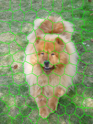
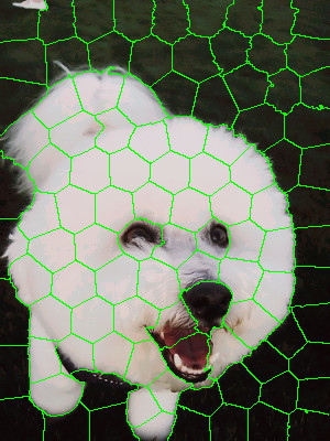
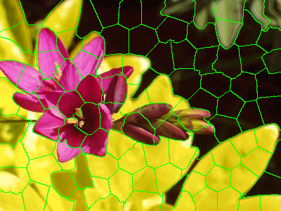
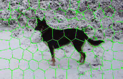
Figure 1: Illustration of SLICO superpixels bounderies: (a) images ; (b) superpixels.

The dissimilarity between pixels of the input color image is then given by the dissimilarity between their feature vectors. We quantify this dissimilarity thanks to the FastMap method which has the interesting property of non-linearly reducing in one dimension these feature vectors while preserving the structure in the data. More precisely, the FastMap allows to find a configuration, in one dimension, that preserves, as much as possible, all the (Euclidean) distance pairs that initially existed between the different (high dimensional) texture vectors (and that takes into account the non-linear distribution of the set of feature vectors). After normalization between the range $0$ and $1$, the map estimated by the FastMap produces the Euclidean embedding (in near-linear time) which can be viewed as a probabilistic map, i.e., with a set of grey levels with high grayscale values for salient regions and low values for non-salient areas.

As Borji and Itti [43] stated, almost all saliency approaches use just one color channel. The latter authors also argued that employing just one color space does not always lead to successful outlier detection. Thus, taking into account this argument, we used, in addition to the RGB color space the color spaces: HSL, LUV and CMY.

Finally, we combine the probabilistic maps obtained from these color spaces to obtain the desired saliency map. To combine the probabilistic maps from the different color spaces used, we reduce for each pixel a vector which is the concatenation of the averages of the values of the superpixel to which this pixel belongs successively in all the color spaces used. In the following section, we describe the different steps in detail.

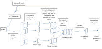
Figure 2: Proposed model steps to obtain the refined probabilistic map from a color space (e.g. RGB).

Image	RR	RG	RB	GR	GG	GB	BR	BG	BB

Figure 3: Micro-texture maps given by LTP on the $9$ opposing color pairs (for the RGB color space). We can notice that this LTP coding already highlight the salient objects.

3.2 LTP Texture Characterization on Opposing Color Pairs

3.2.1 Local Ternary Patterns (LTP)

Since LTP (local ternary patterns) is a kind of generalization of LBP (local binary patterns), let’s first recall the LBP technique.

The local binary pattern $LBP_{P,R}$ labels each pixel of an image (see Eq. 1). The label of a pixel at the position $(x_{c},y_{c})$ with $g_{c}$ as gray level is a set of P binary digits obtained by thresholding each gray level value $g_{p}$ of the $p$ neighbour located at the distance $R$ (see Figure 4) from this pixel by the value of the gray level $g_{c}$ ($p$ is one of the $P$ chosen neighbours). The set of binary digits obtained constitutes the label of this pixel or its LBP code (see Figure 5).

$$\mbox{LBP}_{P,R}(x_{c},y_{c})=\displaystyle\sum_{p=0}^{P-1}s(g_{p}-g_{c})2^{p}$$ (1)

with $(x_{c},y_{c})$ being the pixel coordinate and:

$$s(z)=\begin{cases}1&\quad\text{if }z\geq 0\\ 0&\quad\text{if }z<0\end{cases}$$

Where $z\!=\!g_{p}\!-\!g_{c}$.

Once this code is computed for each pixel, the characterization of the texture of the image (within a neighbourhood) is approximated by a discrete distribution (histogram) of LBP codes of $2^{P}$ bins.

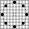
Figure 4: Example of neighbourhood (black disks) for a pixel (central white disk) for $LBP_{P,R}$ code computation : in this case $P=8$, $R=4$.

(a) pixel	(b) after	(c) pattern:	(d)
neighbourhood;	thresholding;	$00001110$	code=14
$g_{c}=239$

Figure 5: Example of LBP code computation for a pixel: LBP code is $2+4+8=14$ in this case.

The LTP (local ternary patterns) [26] is an extension of LBP in which the function $s(z)$ (see Eq. 1) is defined as follows:

$$s(z)=\begin{cases}2&\quad\text{if }z\geq t\\ 1&\quad\text{if }|z|<t\\ 0&\quad\text{if }z\leq-t\end{cases}$$

Where $z\!=\!g_{p}\!-\!g_{c}$.
The basic coding of LTP is, thus expressed as:

$$\mbox{LTP}_{P,R}(x_{c},y_{c})=\displaystyle\sum_{p=0}^{P-1}s(g_{p}-g_{c})3^{p}$$ (2)

Another type of encoding can be obtained by splitting the LTP code into two codes LBP : Upper LBP code and Lower LBP code (see Figure 6). The LTP histogram is then the concatenation of the histogram of the upper LBP code with that of the lower LBP code [26].
In our model we use the LTP basic coding because we use $5$ neighbours for the central pixel. So the maximum size of the histograms is $3^{5}=243$. In addition, we requantized the histogram with levels/classes of $75$ bins for first computational reasons (thus greatly reducing the computational time for the next step using the FastMap algorithm while generalizing the feature vector a bit as this operation smoothes the histogram) and we have effectively noticed that this strategy gives slightly better results.

Figure 6: Example of LTP code splitting with threshold t=3

3.2.2 Opposing Color Pairs

To incorporate the color into the texture description, we rely on the color opponent theory. We thus used color texture descriptor from Mäenpää and Pietikäinen [41, 21] called “Opponent Color LBP”. This one generalizes the classic LBP, which normally applies to grayscale textures. So instead of just one LBP code, one pixel gets a code for every combination of two color channels (i.e., $9$ opposing color pair codes). Example for RGB channels : RR (Red-Red), RG (Red-Green), RB (Red-Blue), GR (Green-Red), GG (Green-Green), GB (Green-Blue), BR (Blue-Red), BG (Blue-Green), BB (Blue-Blue) (see Figure 7). The central pixel is in the first color channel of the combination and the neighbours are picked in the second color (see Figure 8 (b)). The histogram that describes the color micro-texture is the concatenation of the histograms obtained from each opposing color pair.

Figure 7: Illustration of color opponent on RGB (Red Green Blue) color space with its $9$ opposing color pairs (i.e., RR, RG, RB, GR, GG, GB, BR, BG, BB).

(a)	(b)

Figure 8: (a) Pixel gray LBP code: the code for the central pixel (i.e. white small disk) is computed with respect to his neighbours (i.e. 8 black small disks). (b) Pixel opponent color LBP code for RG pair: the central pixel is in the first color channel (red) and the neighbours are picked in the second channel (green).

3.3 FastMap : Multi-Dimensional Scaling

The FastMap [44] is an algorithm which initially was intended to provide a tool allowing to find objects similar to a given object, to find pairs of the most similar objects and to visualize distributions of objects in a desired space in order to be able to identify the main structures in the data, once the similarity or dissimilarity function is determined. This tool remains effective even for large collections of data sets, unlike classical multidimensional scaling (classic MDS). The FastMap algorithm matches objects of a certain dimension to points in a $k$-dimensional space while preserving distances between pairs of objects. This representation of objects from a large-dimensional space $n$ to a smaller-dimensional space (dimension $1$ or $2$ or $3$) allows the visualization of the structures of the distributions in the data or the acceleration of the search time for queries [44].

As Faloutsos and Lin [44] describe it, the problem solved by FastMap can be represented in two ways. First, FastMap can be seen as a mean to represent $N$ objects in a $k$-dimensional space, given the distances between the $N$ objects, while preserving the distances between pairs of objects. Second, the FastMap algorithm can also be used in reducing dimensionality while preserving distances between pairs of vectors. This amounts to finding, given $N$ vectors having $n$ features each, $N$ vectors in a space of dimension $k$ - with $n\gg k$ - while preserving the distances between the pairs of vectors. To do this, the objects are considered as points in the original space. The first coordinate axis is the line that connects the objects called pivots. The pivots are chosen so that the distance separating them is maximum. Thus, to obtain these pivots, the algorithm follows the steps below:

• choose arbitrarily an object as the second pivot, i.e. the object $O_{b}$;

• choose as the first pivot $O_{a}$, the object furthest from $O_{b}$ according to the used distance;

• replace the second pivot with the furthest object from $O_{a}$, that is, the object $O_{b}$;

• return the objects $O_{a}$ and $O_{b}$ as pivots.

The axis of the pivots thus constituting the first coordinate axis in the targeted $k$-dimensional space. All the points representing the objects are then projected orthogonally on this axis and in the H hyperplane of $n-1$ dimensions (perpendicular to the first axis already obtained) connecting the pivot objects $O_{a}$ and $O_{b}$ along the latter axis. The coordinates of a given object $O_{i}$ on the first axis is given by:

$$x_{i}=\frac{d^{2}_{a,i}+d^{2}_{a,b}-d^{2}_{b,i}}{2d_{a,b}}$$ (3)

Where $d_{a,i}$, $d_{b,i}$ and $d_{a,b}$ are respectively the distance between the pivot $O_{a}$ and object $O_{i}$, the distance between the pivot $O_{b}$ and object $O_{i}$, the distance between the pivot $O_{a}$ and the pivot $O_{b}$. The process is repeated up to the desired dimension, each time expressing:

1. the new distance $D^{\prime}()$:

   $$(D^{\prime}(O^{\prime}_{i},O^{\prime}_{j}))^{2}=(D(O_{i},O_{j}))^{2}-(x_{i}-x_{j})^{2}$$ (4)

   For simplification,

   $$D^{\prime}(O^{\prime}_{i},O^{\prime}_{j})\equiv d^{\prime}_{O^{\prime}_{i},O^{\prime}_{j}}$$

   Where $x_{i}$ and $x_{j}$ are the coordinates on the previous axis of respectively the object $O_{i}$ and $O_{j}$.

2. the new pivots $O^{\prime}_{a}$ and $O^{\prime}_{b}$ constituting the new axis,

3. the coordinate of the projected object $O^{\prime}_{i}$ on the new axis:

   $$x^{\prime}_{i}=\frac{d^{\prime 2}_{a^{\prime},i}+d^{\prime 2}_{a^{\prime},b^{\prime}}-d^{\prime 2}_{b^{\prime},i}}{2d^{\prime}_{a^{\prime},b^{\prime}}}$$ (5)

$O_{a^{\prime}}$ and $O_{b^{\prime}}$ are the new pivots according to the new distance expression $D^{\prime}()$. The line that connects them is therefore the new axis.

After normalization between the range $0$ and $1$, the map estimated by the FastMap generates a probabilistic map, i.e., with a set of grey levels with high grayscale values for salient regions and low values for non-salient areas. Nevertheless, in some (rare) cases, the map estimated by the FastMap algorithm, can possibly present a set of grey levels whose amplitude values would be in the complete opposite direction (i.e., low grayscale values for salient regions and high values for non-salient areas). In order to put this grayscale mapping in the right direction (with high grayscale values associated with salient objects), we simply use the fact that a salient object/region is more likely to appear in the center of the image (or conversely unlikely on the edges of the image). To this end, we compute the Pearson correlation coefficient between the saliency map obtained by the FastMap and a rectangle, with maximum intensity value and about half the size of the image, and located in the center of the image. If the correlation coefficient is negative (anti-correlation), we invert the signal (i.e., associate to each pixel its complementary gray value).

NUMBER	1	2	3	4	5	6	7	8	9	10
IMAGE
GT
CHS[45]
HS[46]
OURS

Figure 9: Comparison of some result images for HS[46], CHS[45] and our model. For image number 8, the HS[46] and CHS[45] models find white salient maps (GT: Ground Truth).

4 Experimental Results

In this section, we present our salient objects detection model’s results. In order to obtain the LTP_P,R pixel’s code (LTP code for simplification), we used an adaptive threshold. Let a pixel at position $(x_{c},y_{c})$ with value $g_{c}$, the threshold for its LTP code is the tenth of the pixel’s value: $t=\frac{g_{c}}{10}$ (see Eq. 2). We chose this threshold because empirically it is this value that has given better results. The number of neighbours P around the pixel on a radius R used to find its LTP code in our model is $P=5$ and $R=1$. Thus the maximum value of the LTP code in our case is $3^{5}-1=242$. This makes the maximum size of the histogram characterizing the micro-texture in an opposing color pair to be $3^{5}=243$ which is then requantized with levels/classes of 75 bins (see Section 3.2). The superpixels that we use as adaptive windows to characterize the color micro-textures are obtained thanks to SLICO (Simple Linear Iterative Clustering with zero parameter) algorithm which is faster and exhibits state-of-the-art boundary adherence. Its only parameter is the number of superpixels desired and is set to $100$ in our model (which is also the value recommended by the author of the SLICO algorithm). Finally, we use in the combination to obtain the final saliency map the color spaces RGB, HSL, LUV and CMY. We chose, for our experiments, images from public datasets, the most widely used in the salient objects detection field [40] such as Extended Complex Scene Saliency Dataset (ECSSD) and Microsoft Research Asia 10,000 (MSRA10K). The ECSSD contains $1000$ natural images and their ground truth. Many of its images are semantically meaningful, but structurally complex for saliency detection [45]. The MSRA10K contains $10\,000$ images and $10\,000$ manually obtained binary saliency maps corresponding to their ground truth [35, 40].

Table 1: Our model’s $F_{\beta}$ measure and MAE results for ECSSD and MSRA10K datasets.

	ECSSD	MSRA10K
$F_{\beta}$ measure	$0.729$	$0.781$
MAE	$0.257$	$0.222$

Table 2: Our model’s $F_{\beta}$ measure and MAE results compared with some state-of-the-art models from Borji et al. [40] for ECSSD dataset (for MAE, the smaller value is the best).

	AC [34]	CA[38]	HC[35]	HS[46]	OURS
MAE	$0.265$	$0.310$	$0.331$	$0.228$	$0.257$
$F_{\beta}$	$0.411$	$0.515$	$0.460$	$0.731$	$0.729$

Our saliency maps are of good quality (see Figure 9).) as shown by the visual comparison with some of them and two state-of-the-art models (“Hierarchical saliency detection”: HS[46] and “Hierarchical image saliency detection on extended CSSD”: CHS[45] models). We used for evaluation of our salient objects detection model the Mean Absolute Error (MAE), the Precision-Recall curve (PR), $F_{\beta}$ measure curve and the $F_{\beta}$ measure with $\beta^{2}=0.3$. Table 1 shows the $F_{\beta}$ measure and the Mean Absolute Error (MAE) of our model on ECSSD and MSRA10K datasets.

Our results also show that combining the opposing color pairs improves the individual contribution of each pair to the F_β measure and the Precision-Recall as shown for the RGB color space by the F_β measure curve (Figure 10) and the Precision-Recall curve (Figure 11). The combination of the color spaces RGB, HSL, LUV and CMY improves also the final result as it can be seen on the $F_{\beta}$ measure curve and the precision-recall curve (see Figure 12 and Figure 13).

We compared the MAE (Mean Absolute Error) and F_β measure of our model with the $29$ state-of-the-art models from Borji et al.[40] and our model outperformed $11$ models. Table 2 shows the MAE (Mean Absolute Error) and F_β measures values for the ECSSD dataset of some models. Finally, we compared our model with the two state-of-the-art HS[46] and CHS [45] models with respect to the precision-recall and F_β measure curves. We see that our model still performs well (see Figure 14 and Figure 15).

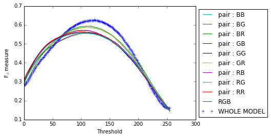
Figure 10: $F_{\beta}$ measure curves for opposing color pairs, RGB color space and the whole model on ECSSD dataset.

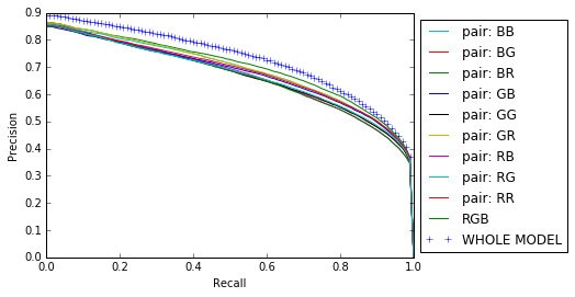
Figure 11: Precision-Recall curves for opposing color pairs, RGB color space and the whole model on ECSSD dataset.

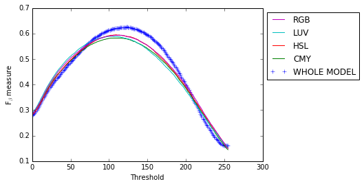
Figure 12: $F_{\beta}$ measure curves for color spaces RGB, HSL, LUV and CMY and the whole model on ECSSD dataset.

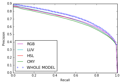
Figure 13: Precision-Recall curves for color spaces RGB, HSL, LUV and CMY and the whole model on ECSSD dataset.

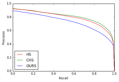
Figure 14: Precision-Recall curves for HS[46], CHS [45] models and ours on ECSSD dataset.

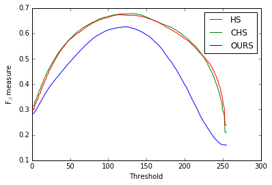
Figure 15: $F_{\beta}$ measure curves for HS [46], CHS [45] models and ours on ECSSD dataset.

5 Discussion

Our model has less dispersed MAE measures than the HS[46] and CHS[45] models which are among the best models of the state-of-the-art. This can be observed in Figure 16 but also shown by the standard deviation which for our model is 0.071 (mean = 0.257), for HS[46] is 0.108 (mean = 0.227), for CHS[45] is 0.117 (mean = 0.226). For HS[46] the relative error between the two standard deviations is $\frac{(0.108-0.071)\times 100}{0.071}=52.11\%$ while for CHS[45] is $\frac{(0.117-0.071)\times 100}{0.071}=64.78\%$.

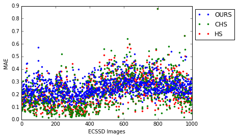
Figure 16: Comparison of the MAE measure dispersion for our model and the HS [46], CHS [45] models on ECSSD dataset (for MAE, the smaller value is the best).

Our model is stable on new data. Indeed, a model with very few internal parameters is supposed to be more stable for different datasets. Also, we noticed that nearly 500 first image numbers of the ECSSD dataset are less complex than the rest of the images in this dataset by observing the different measures (see Table 3 and Figure 16 and Figure 17). But it is clear that the drop in performance over the last 500 images from the ECSSD dataset is less pronounced for our model than for the HS [46] and CHS [45] models (see Table 3). This can be explained by the stability of our model (we used to compute these measures except for MAE a threshold, for each image, which gives the best $F_{\beta}$ measure. It should also be noted that the images are ordered only by their numbers in the ECSSD dataset).

Table 3: Performance drop for Precision and MAE measures with respect to image numbers 0 to 500(*) and 500 to 1000(**) of the ECSSD dataset (for MAE, the smaller value is the best).

	Precision			MAE
	ours	HS	CHS	ours	HS	CHS
(*)	0.832	0.919	0.921	0.234	0.176	0.172
(**)	0.737	0.791	0.791	0.279	0.278	0.280
Gap	0.095	0.128	0.130	0.045	0.102	0.108

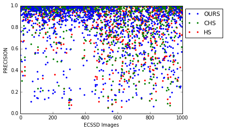
Figure 17: Comparison of the precision measure dispersion for our model and the HS [46], CHS [45] models on ECSSD dataset.

Our model is also relatively stable for an increase or decrease of its unique internal parameter. Indeed, by increasing or decreasing the number of superpixels, which is the only parameter of the SLICO algorithm, we find that there is almost no change in the results as shown by the MAE and $F_{\beta}$ measure (see Table 4) and $F_{\beta}$ measure and precision-recall curves for 50, 100 and 200 superpixels (see Figure 18 and Figure 19).

Table 4: Our model’s $F_{\beta}$ measure and MAE results for 50, 100 and 200 superpixels (ECSSD dataset).

Superpixels	50	100	200
$F_{\beta}$ measure	$0.722$	$0.729$	$0.725$
MAE	$0.257$	$0.257$	$0.257$

Figure 18: Precision-Recall model’s curves for 50, 100, 200 superpixels (ECSSD dataset).

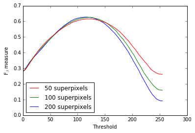
Figure 19: $F_{\beta}$ measure model’s curves for 50, 100, 200 superpixels (ECSSD dataset).

6 Conclusions

In this work, we presented a simple nearly parameter-free model for the estimation of saliency maps. We tested our model on the complex ECSSD dataset and on the MSRA10K dataset on which the average measures of MAE = $0.257$ and F_β measure = $0.729$.
The novelty of our model is that it only uses the textural feature after incorporating the color information into these textural features thanks to the opposing color pairs theory of a given color space. This is made possible by the LTP (Local Ternary Patterns) texture descriptor which, being an extension of LBP (Local Binary Patterns), inherits its strengths while being less sensitive to noise in uniform regions. Thus, we characterize each pixel of the image by a feature vector given by a color micro-texture obtained thanks to SLICO superpixel algorithm. In addition, the FastMap algorithm reduces each of these feature vectors to one dimension while taking into account the non-linearities of these vectors and preserving their distances. This means that our saliency map combines local and global approaches in a single approach and does so in almost linear complexity times.
In our model, we used RGB, HSL, LUV and CMY color spaces. Our model is therefore perfectible if we increase the number of color spaces (uncorrelated) to be merged.
As shown by the results we obtained, this strategy generates a model which is very promising, since it is quite different from existing saliency detection methods using the classical color contrast strategy between a region and the other regions of the image and consequently it could thus be efficiently combined with these methods for better performance. In addition, it should be noted that this strategy of integrating color into local textural patterns could also be interesting to study with deep learning techniques or convolutional neural networks (CNNs) to further improve the quality of saliency maps.

References

- [1] Derrick Parkhurst, Klinton Law, and Ernst Niebur. Modeling the role of salience in the allocation of overt visual attention. Vision research, 42(1):107–123, 2002.
- [2] Laurent Itti. Models of bottom-up attention and saliency. In Neurobiology of attention, pages 576–582. Elsevier, 2005.
- [3] Laurent Itti and Christof Koch. Computational modelling of visual attention. Nature reviews neuroscience, 2(3):194–203, 2001.
- [4] Farhan Baluch and Laurent Itti. Mechanisms of top-down attention. Trends in neurosciences, 34(4):210–224, 2011.
- [5] Anne Treisman. Features and objects: The fourteenth bartlett memorial lecture. The quarterly journal of experimental psychology, 40(2):201–237, 1988.
- [6] Jeremy M Wolfe, Kyle R Cave, and Susan L Franzel. Guided search: an alternative to the feature integration model for visual search. Journal of Experimental Psychology: Human perception and performance, 15(3):419, 1989.
- [7] Christof Koch and Shimon Ullman. Shifts in selective visual attention: towards the underlying neural circuitry. In Matters of intelligence, pages 115–141. Springer, 1987.
- [8] Ali Borji, Ming-Ming Cheng, Qibin Hou, Huaizu Jiang, and Jia Li. Salient object detection: A survey. Computational visual media, pages 1–34.
- [9] Ali Borji and Laurent Itti. State-of-the-art in visual attention modeling. IEEE transactions on pattern analysis and machine intelligence, 35(1):185–207, 2012.
- [10] Laurent Itti. Automatic foveation for video compression using a neurobiological model of visual attention. IEEE transactions on image processing, 13(10):1304–1318, 2004.
- [11] Jinjiang Li, Xiaomei Feng, and Hui Fan. Saliency-based image correction for colorblind patients. Computational Visual Media, 6(2):169–189, 2020.
- [12] Yuan Gao, Miaojing Shi, Dacheng Tao, and Chao Xu. Database saliency for fast image retrieval. IEEE Transactions on Multimedia, 17(3):359–369, 2015.
- [13] Rik Pieters and Michel Wedel. Attention capture and transfer in advertising: Brand, pictorial, and text-size effects. Journal of Marketing, 68(2):36–50, 2004.
- [14] Lai-Kuan Wong and Kok-Lim Low. Saliency-enhanced image aesthetics class prediction. In 2009 16th IEEE International Conference on Image Processing (ICIP), pages 997–1000. IEEE, 2009.
- [15] Hantao Liu and Ingrid Heynderickx. Studying the added value of visual attention in objective image quality metrics based on eye movement data. In 2009 16th IEEE international conference on image processing (ICIP), pages 3097–3100. IEEE, 2009.
- [16] Li-Qun Chen, Xing Xie, Xin Fan, Wei-Ying Ma, Hong-Jiang Zhang, and He-Qin Zhou. A visual attention model for adapting images on small displays. Multimedia systems, 9(4):353–364, 2003.
- [17] Tao Chen, Ming-Ming Cheng, Ping Tan, Ariel Shamir, and Shi-Min Hu. Sketch2photo: Internet image montage. ACM transactions on graphics (TOG), 28(5):1–10, 2009.
- [18] Zuyi Yang, Qinghui Dai, and Junsong Zhang. Visual perception driven collage synthesis. Computational Visual Media, 8(1):79–91, 2022.
- [19] Hua Huang, Lei Zhang, and Hong-Chao Zhang. Arcimboldo-like collage using internet images. In Proceedings of the 2011 SIGGRAPH Asia Conference, pages 1–8, 2011.
- [20] Arnold WM Smeulders, Dung M Chu, Rita Cucchiara, Simone Calderara, Afshin Dehghan, and Mubarak Shah. Visual tracking: An experimental survey. IEEE transactions on pattern analysis and machine intelligence, 36(7):1442–1468, 2013.
- [21] Matti Pietikäinen, Abdenour Hadid, Guoying Zhao, and Timo Ahonen. Computer vision using local binary patterns, volume 40. Springer Science & Business Media, 2011.
- [22] Mark Haidekker. Advanced biomedical image analysis. John Wiley & Sons, 2011.
- [23] H. Knutsson and G Granlund. Texture analysis using two-dimensional quadrature filters. In IEEE Comput. Soc. Workshop on Computer Architecture for Pattern Analysis and Image Database Management, pages 206–213, 1983.
- [24] Timo Ojala, Matti Pietikäinen, and David Harwood. A comparative study of texture measures with classification based on featured distributions. Pattern recognition, 29(1):51–59, 1996.
- [25] Kenneth I Laws. Textured image segmentation. PhD thesis, University of Southern California Los Angeles Image Processing INST, 1980.
- [26] Xiaoyang Tan and Bill Triggs. Enhanced local texture feature sets for face recognition under difficult lighting conditions. IEEE transactions on image processing, 19(6):1635–1650, 2010.
- [27] Ran Margolin, Ayellet Tal, and Lihi Zelnik-Manor. What makes a patch distinct? In Proceedings of the IEEE conference on computer vision and pattern recognition, pages 1139–1146, 2013.
- [28] Qing Zhang, Jiajun Lin, Yanyun Tao, Wenju Li, and Yanjiao Shi. Salient object detection via color and texture cues. Neurocomputing, 243:35–48, 2017.
- [29] Alice Porebski, Nicolas Vandenbroucke, and Ludovic Macaire. Haralick feature extraction from lbp images for color texture classification. In 2008 First Workshops on Image Processing Theory, Tools and Applications, pages 1–8. IEEE, 2008.
- [30] Anne M Treisman and Garry Gelade. A feature-integration theory of attention. Cognitive psychology, 12(1):97–136, 1980.
- [31] Jeremy M Wolfe and Todd S Horowitz. What attributes guide the deployment of visual attention and how do they do it? Nature reviews neuroscience, 5(6):495–501, 2004.
- [32] Laurent Itti, Christof Koch, and Ernst Niebur. A model of saliency-based visual attention for rapid scene analysis. IEEE Transactions on pattern analysis and machine intelligence, 20(11):1254–1259, 1998.
- [33] Simone Frintrop, Thomas Werner, and German Martin Garcia. Traditional saliency reloaded: A good old model in new shape. In Proceedings of the IEEE conference on computer vision and pattern recognition, pages 82–90, 2015.
- [34] Radhakrishna Achanta, Francisco Estrada, Patricia Wils, and Sabine Süsstrunk. Salient region detection and segmentation. In International conference on computer vision systems, pages 66–75. Springer, 2008.
- [35] Ming-Ming Cheng, Niloy J Mitra, Xiaolei Huang, Philip HS Torr, and Shi-Min Hu. Global contrast based salient region detection. IEEE Transactions on Pattern Analysis and Machine Intelligence, 37(3):569–582, 2015.
- [36] Chenlei Guo and Liming Zhang. A novel multiresolution spatiotemporal saliency detection model and its applications in image and video compression. IEEE transactions on image processing, 19(1):185–198, 2009.
- [37] Federico Perazzi, Philipp Krähenbühl, Yael Pritch, and Alexander Hornung. Saliency filters: Contrast based filtering for salient region detection. In Computer Vision and Pattern Recognition (CVPR), 2012 IEEE Conference on, pages 733–740. IEEE, 2012.
- [38] Stas Goferman, Lihi Zelnik-Manor, and Ayellet Tal. Context-aware saliency detection. IEEE transactions on pattern analysis and machine intelligence, 34(10):1915–1926, 2012.
- [39] Wei Qi, Ming-Ming Cheng, Ali Borji, Huchuan Lu, and Lian-Fa Bai. Saliencyrank: Two-stage manifold ranking for salient object detection. Computational Visual Media, 1(4):309–320, 2015.
- [40] Ali Borji, Ming-Ming Cheng, Huaizu Jiang, and Jia Li. Salient object detection: A benchmark. IEEE transactions on image processing, 24(12):5706–5722, 2015.
- [41] Topi Mäenpää and Matti Pietikäinen. Classification with color and texture: jointly or separately? Pattern recognition, 37(8):1629–1640, 2004.
- [42] Radhakrishna Achanta, Appu Shaji, Kevin Smith, Aurelien Lucchi, Pascal Fua, and Sabine Süsstrunk. Slic superpixels compared to state-of-the-art superpixel methods. IEEE transactions on pattern analysis and machine intelligence, 34(11):2274–2282, 2012.
- [43] Ali Borji and Laurent Itti. Exploiting local and global patch rarities for saliency detection. In 2012 IEEE conference on computer vision and pattern recognition, pages 478–485. IEEE, 2012.
- [44] Christos Faloutsos and King-Ip Lin. FastMap: A fast algorithm for indexing, data-mining and visualization of traditional and multimedia datasets, volume 24. ACM, 1995.
- [45] Jianping Shi, Qiong Yan, Li Xu, and Jiaya Jia. Hierarchical image saliency detection on extended cssd. IEEE transactions on pattern analysis and machine intelligence, 38(4):717–729, 2016.
- [46] Qiong Yan, Li Xu, Jianping Shi, and Jiaya Jia. Hierarchical saliency detection. In Proceedings of the IEEE conference on computer vision and pattern recognition, pages 1155–1162, 2013.