Exact scalar (quasi-)normal modes of black holes and solitons in gauged SUGRA

Abstract

In this paper we identify a new family of black holes and solitons that lead to the exact integration of scalar probes, even in the presence of a non-minimal coupling with the Ricci scalar which has a non-trivial profile. The backgrounds are planar and spherical black holes as well as solitons of $SU\left(2\right)\times SU\left(2\right)$ $\mathcal{N}=4$ gauged supergravity in four dimensions. On these geometries, we compute the spectrum of (quasi-)normal modes for the non-minimally coupled scalar field. We find that the equation for the radial dependence can be integrated in terms of hypergeometric functions leading to an exact expression for the frequencies. The solutions do not asymptote to a constant curvature spacetime, nevertheless the asymptotic region acquires an extra conformal Killing vector. For the black hole, the scalar probe is purely ingoing at the horizon, and requiring that the solutions lead to an extremum of the action principle we impose a Dirichlet boundary condition at infinity. Surprisingly, the quasinormal modes do not depend on the radius of the black hole, therefore this family of geometries can be interpreted as isospectral in what regards to the wave operator non-minimally coupled to the Ricci scalar. We find both purely damped modes, as well as exponentially growing unstable modes depending on the values of the non-minimal coupling parameter. For the solitons we show that the same integrability property is achieved separately in a non-supersymmetric solutions as well as for the supersymmetric one. Imposing regularity at the origin and a well defined extremum for the action principle we obtain the spectra that can also lead to purely oscillatory modes as well as to unstable scalar probes, depending on the values of the non-minimal coupling.

I Introduction

Quasinormal modes play a very important role both in astrophysical as well as in theoretical contexts. In the former, they dominate the ringdown dynamics of the final black hole obtained from the fusion of compact objects, and a direct measurement of the mode with the lowest damping helps obtaining the mass and angular momentum of the final object LIGOScientific:2016aoc . In the latter, black hole quasinormal modes, within the context of holography, allow for the computation of relaxation properties of the dual field theory living at the boundary of AdS Horowitz:1999jd ,Birmingham:2001pj . It is well-known that even for simple black holes, as for example for Schwarzschild-(A)dS the computation of quasinormal modes relies on numerical techniques. These techniques are fully reliable, notwithstanding there are particular interesting cases where the spectrum of quasinormal frequencies can be found analytically which are useful to explore the relaxation properties of perturbations outside a black hole in an exact manner as one modifies the parameters that define the background geometry. A partial list of such cases is given by Chan:1996yk -Chernicoff:2020kmf . In this paper, we identify a new family of black holes and solitons that allow for the exact integration of non-minimally coupled scalar probes, in the context of $SU\left(2\right)\times SU\left(2\right)$ $\mathcal{N}=4$ gauged supergravity in four dimensions. This theory, also known as the Freedman-Schwarz FS model can be obtained from 10D supergravity compactified on $S^{3}\times S^{3}$ CVcorto , CVlargo . The action principle reads

$$S =\int d^{4}x\sqrt{-g}\left[\frac{R}{4}-\frac{1}{2}\partial_{\mu}\phi\partial^{\mu}\phi-\frac{1}{2}e^{4\phi}\partial_{\mu}a\partial^{\mu}a+\frac{e_{A}^{2}+e_{B}^{2}}{8}e^{2\phi}-\frac{e^{-2\phi}}{4}\left(A^{i\mu\nu}A_{i\mu\nu}+B^{i\mu\nu}B_{i\mu\nu}\right)\right.$$

$$\left.-\frac{\mathbf{a}}{4}\frac{\epsilon^{\mu\nu\rho\sigma}}{\sqrt{-g}}\left(A_{i\mu\nu}A_{\ \rho\sigma}^{i}+B_{i\mu\nu}B_{\ \rho\sigma}^{i}\right)\right]$$ (1)

and the axion field $\mathbf{a}$ can consistently be set to zero provided the following equation of Pontryagin densities for the $SU\left(2\right)$ gauge fields holds

$$\epsilon^{\mu\nu\rho\sigma}\left(A_{i\mu\nu}A_{\ \rho\sigma}^{i}+B_{i\mu\nu}B_{\ \rho\sigma}^{i}\right)=0\ .$$ (2)

The field strength for the gauge fields are given by

$$A_{\mu\nu}^{i}=\partial_{\mu}A_{\nu}^{i}-\partial_{\nu}A_{\mu}^{i}+e_{A}\epsilon_{ijk}A_{\mu}^{j}A_{\nu}^{k}\text{\qquad and\qquad}B_{\mu\nu}^{i}=\partial_{\mu}B_{\nu}^{i}-\partial_{\nu}B_{\mu}^{i}+e_{B}\epsilon_{ijk}B_{\mu}^{j}B_{\nu}^{k}\ .$$ (3)

In this work we will focus on the computation of quasinormal modes of scalar probes on black holes of this theory as well as on the computation of normal frequencies of the same probe fields on the gravitational soliton recently constructed in Canfora:2021nca , both in the supersymmetric and non-supersymmetric cases. We will deal with solutions with vanishing axion field, and since the self-interaction of the dilaton does not have a local extremum, the solutions have an asymptotic structure that has less symmetry than a maximally symmetric spacetime, although we will see the emergence of an asymptotic conformal Killing vector.

II Scalar probes on black holes

The two families of black holes we will be interested in this section were constructed in Klemm . The metric in both cases, namely spherical and planar, reads

$$ds^{2}=-\alpha r^{2}\left(1-\frac{r_{+}^{2}}{r^{2}}\right)dt^{2}+\frac{dr^{2}}{\alpha\left(1-\frac{r_{+}^{2}}{r^{2}}\right)}+r^{2}d\Sigma_{2}^{2}\ ,$$ (4)

where $\Sigma_{2}$ is a two-dimensional Euclidean manifold of constant curvature $\gamma=+1,0$.

In the spherically symmetric case, $\gamma=+1$ and $d\Sigma_{2}^{2}=d\theta^{2}+\sin^{2}\theta d\varphi^{2}$ is the line element of the round two-sphere, while the constant $\alpha$, the dilaton and gauge fields read

$$\alpha =\frac{1}{2}\left(e_{A}^{2}+e_{B}^{2}\right)\left(H_{A}^{2}+H_{B}^{2}\right)+\frac{1}{4}\ ,$$ (5)

$$\phi\left(r\right) =-\ln\left(\frac{r}{2\sqrt{H_{A}^{2}+H_{B}^{2}}}\right)\ ,$$ (6)

$$A_{\left[1\right]}^{i} =-H_{A}\cos\theta d\varphi\delta_{3}^{i}\ ,$$ (7)

$$B_{\left[1\right]}^{i} =-H_{B}\cos\theta d\varphi\delta_{3}^{i}\ .$$ (8)

In the planar case, $\gamma=0$, $d\Sigma_{2}^{2}=dx^{2}+dy^{2}$ the gauge fields vanish and

$$\alpha=\frac{e_{A}^{2}+e_{B}^{2}}{8}\ ,$$ (9)

$$\phi\left(r\right)=-\ln\left(r\right)\ .$$ (10)

The black holes (4) approach the background

$$ds_{\text{back}}^{2}=-\alpha r^{2}dt^{2}+\frac{dr^{2}}{\alpha}+r^{2}d\Sigma_{2}^{2}\ ,$$ (11)

with the following asymptotic behavior

$$\delta g_{tt}=\mathcal{O}\left(1\right)\text{, }\delta g_{rr}=\mathcal{O}\left(r^{-2}\right)\ .$$ (12)

Notice that the background (11) has an extra conformal Killing vector generated by $r\rightarrow\lambda r$. The temperature of this black hole has the intriguing property of being independent of the $r_{+}$, namely a constant, and it is given by

$$T=\frac{\alpha}{2\pi}\ .$$ (13)

As we show below, a similar feature occurs with the quasinormal frequencies of the non-minimally coupled scalar on this geometry, which do not depend on $r_{+}$, leading to isospectral geometries in what regards to such operator. Wald’s formula for the entropy yields

$$S=\frac{A}{4G}=\pi r_{+}^{2}\text{Vol}\left(\Sigma\right)\ ,$$ (14)

where Vol$\left(\Sigma\right)$ is the volume of the Euclidean manifold $\Sigma_{2}$ and we have normalized the Einstein term in the action (1) such that $G=(4\pi)^{-1}$. First law

$$dM=TdS\ ,$$ (15)

provides the following value for the mass of the black hole

$$M=\frac{\alpha r_{+}^{2}\text{Vol}\left(\Sigma\right)}{2}\ .$$ (16)

Here, as an avatar for the study of the stability of these black holes, we will consider a real scalar probe, coupled to the Ricci scalar in a non-minimal manner:

$$\square\Phi-\xi R\Phi=0\ ,$$ (17)

on the background (4).

Given the local isometries of the spacetime, the scalar probe admits a mode separation which is given by

$$\Phi\left(t,r,y^{i}\right)=\operatorname{Re}\left(\int d\omega\sum_{A}e^{-i\omega t}H_{\omega,A}\left(r\right)Y_{A}\left(y\right)\right)\ ,$$ (18)

where $y^{i}$ are the coordinates on the Euclidean manifold $\Sigma_{2}$ and $Y_{k}\left(y\right)$ are harmonic function on such manifold, which are labeled by the multi-index $A$. Concretely, for the spherically symmetric case the harmonic functions are standard spherical harmonics, namely $A=\left\{l,m\right\}$ and they fulfil

$$\nabla_{S^{2}}^{2}Y_{l,m}=-k^{2}Y_{l,m}=-l\left(l+1\right)Y_{l,m}\ ,$$ (19)

while for the planar case, the harmonic functions are trivially given by plane waves of the form

$$Y_{A}=Y_{\vec{k}}=Ce^{-i\vec{k}\cdot\vec{y}}\ ,$$ (20)

which fulfil

$$\nabla_{R^{2}}Y_{\vec{k}}=-k^{2}Y_{\vec{k}}=-\left(k_{1}^{2}+k_{2}^{2}\right)Y_{\vec{k}}\ .$$ (21)

Hereafter, for brevity we introduce the notation $H_{\omega,A}\left(r\right)=H\left(r\right)$.

Notice that since the Ricci scalar of the spacetime has a non-trivial radial profile

$$R=\frac{2\gamma-6\alpha}{r^{2}}-\frac{2\alpha r_{+}^{2}}{r^{4}}\ ,$$ (22)

the non-minimal coupling term in (17) cannot be seen as an effective mass term. In spite of this fact, we will show that the equation for the radial profile of the scalar probe $H\left(r\right)$ can be solved in an exact manner in terms of hypergeometric functions.

Introducing the separation (18) on the scalar field equation (17) as a probe field on the black hole metric (4), after performing the change of variables

$$r=\frac{r_{+}}{\left(1-x\right)^{1/2}}\ ,$$ (23)

which maps the region of outer communication $r\in[r_{+},+\infty[$ to $x\in[0,1[$, leads to the following equation for the radial profile

$$\frac{d^{2}H\left(x\right)}{dx^{2}}+\frac{1}{x}\frac{dH\left(x\right)}{dx}+\left(\frac{\omega^{2}}{4\alpha^{2}x^{2}\left(1-x\right)^{2}}-\frac{k^{2}}{4\alpha x\left(1-x\right)^{2}}-\frac{(\alpha x-4\alpha+\gamma)}{2\alpha x\left(1-x\right)^{2}}\xi\right)H\left(x\right)=0\ .$$ (24)

Remarkably, this equation admits a solution in terms of hypergeometric functions. After imposing ingoing boundary condition at the horizon one obtains

$$H\left(x\right)=C_{1}x^{-\frac{i\omega}{2\alpha}}(1-x)^{\frac{\alpha+\sqrt{\left(1-6\xi\right)\alpha^{2}+2\xi\alpha\gamma+\alpha k^{2}-\omega^{2}}}{2\alpha}}F\left(a_{1},b_{1},c_{1},x\right)\ ,$$ (25)

with

$$a_{1} =\frac{1}{2}-\frac{i\omega}{2\alpha}-\frac{\sqrt{2\xi}}{2}+\frac{\sqrt{\left(1-6\xi\right)\alpha^{2}+2\xi\alpha\gamma+\alpha k^{2}-\omega^{2}}}{2\alpha}\ ,$$ (26)

$$b_{1} =\frac{1}{2}-\frac{i\omega}{2\alpha}+\frac{\sqrt{2\xi}}{2}+\frac{\sqrt{\left(1-6\xi\right)\alpha^{2}+2\xi\alpha\gamma+\alpha k^{2}-\omega^{2}}}{2\alpha}\ ,$$ (27)

$$c_{1} =1-\frac{i\omega}{\alpha}\ .$$ (28)

Using Kummer identities, the ingoing solution (25) can be rewritten as

$$H\left(x\right) =C_{1}x^{-\frac{i\omega}{2\alpha}}(1-x)^{\frac{\alpha+\sqrt{\left(1-6\xi\right)\alpha^{2}+2\xi\alpha\gamma+\alpha k^{2}-\omega^{2}}}{2\alpha}}\left[\frac{\Gamma\left(c_{1}\right)\Gamma\left(c_{1}-a_{1}-b_{1}\right)}{\Gamma\left(c_{1}-a_{1}\right)\Gamma\left(c_{1}-b_{1}\right)}F\left(a_{1},b_{1},a_{1}+b_{1}+1-c_{1},1-x\right)\right.$$

$$\left.+\left(1-x\right)^{c_{1}-a_{1}-b_{1}}\frac{\Gamma\left(c_{1}\right)\Gamma\left(a_{1}+b_{1}-c_{1}\right)}{\Gamma\left(a_{1}\right)\Gamma\left(b_{1}\right)}F\left(c_{1}-a_{1},c_{1}-b_{1},1+c_{1}-a_{1}-b_{1},1-x\right)\right]\ ,$$ (29)

which near infinity, as a function of the radial coordinate $r$, leads to

$$H\left(r\right)\sim_{r\rightarrow\infty}\frac{A_{bh}}{r^{\eta_{+}}}\left(1+O\left(\frac{1}{r}\right)\right)+\frac{B_{bh}}{r^{\eta_{-}}}\left(1+O\left(\frac{1}{r}\right)\right)$$ (30)

where

$$A_{bh} =\frac{\Gamma\left(c_{1}\right)\Gamma\left(c_{1}-a_{1}-b_{1}\right)}{\Gamma\left(c_{1}-a_{1}\right)\Gamma\left(c_{1}-b_{1}\right)}\ ,$$ (31)

$$B_{bh} =\frac{\Gamma\left(c_{1}\right)\Gamma\left(a_{1}+b_{1}-c_{1}\right)}{\Gamma\left(a_{1}\right)\Gamma\left(b_{1}\right)}\ ,$$ (32)

and

$$\eta_{\pm}=1\pm\sqrt{(1-6\xi)+\frac{(2\gamma\xi+k^{2})}{\alpha}-\frac{\omega^{2}}{\alpha^{2}}}\ .$$ (33)

This implies that different modes will have polynomial asymptotic expansions at infinity in the radial coordinate, with an exponent that is frequency dependent. This is in contrast with the asymptotically flat case for which $R\left(r\right)\sim e^{\pm i\omega r}$, and with the asymptotically AdS case for which $\eta_{\pm}=\Delta_{\pm}$ being independent of both the angular momentum $k$ and the frequency $\omega$. Since in general $\omega\in\mathbb{C}$, in order to understand the possible boundary conditions at infinity, we will require the action principle to attain an extremum on the family of solutions that are ingoing at the horizon. The action principle leading to (17) reads

$$I=\int d^{4}x\sqrt{-g}\left(-\frac{1}{2}\nabla_{\mu}\Phi\nabla^{\mu}\Phi-\frac{1}{2}\xi R\Phi^{2}\right)\ ,$$ (34)

and its on-shell variation with respect to the scalar field leads to the boundary term

$$\delta I=-\int_{M}d^{4}x\sqrt{-g}\nabla_{\mu}\left(\nabla^{\mu}\Phi\delta\Phi\right)=-\int_{\partial M}d^{3}x\sqrt{-\gamma}\hat{n}_{\mu}\nabla^{\mu}\Phi\delta\Phi\ ,$$ (35)

where $\gamma$ is the determinant of the induced metric on the boundary, while $\hat{n}_{\mu}$ is its unit normal vector. The boundary is the union of the spatial surfaces at $t=t_{i}$ and $t=t_{f}$, with the surface $r=r_{0}$ with $r_{0}\rightarrow\infty$. As usual, the contribution of the former vanish since we impose $\delta\Phi\left(t_{i},r,y\right)=\delta\Phi\left(t_{f},r,y\right)=0$, while the latter leads to

$$-\lim_{r_{0}\rightarrow\infty}r^{3}\partial_{r}H\delta H|_{r=r_{0}}=\lim_{r_{0}\rightarrow\infty}\left.\frac{\eta_{+}A_{bh}^{2}}{r^{2\eta_{+}-2}}+\frac{\eta_{-}B_{bh}^{2}}{r^{2\eta_{-}-2}}+\frac{A_{bh}B_{bh}\left(\eta_{+}+\eta_{-}\right)}{r^{\eta_{+}+\eta_{-}-2}}\right|_{r=r_{0}}\delta C_{1}$$ (36)

One can check that $\eta_{+}+\eta_{-}-2$ vanishes, while $\operatorname{Re}\left(2\eta_{-}-2\right)<0$ and $\operatorname{Re}\left(2\eta_{+}-2\right)>0$ on the whole complex $\omega$-plane, therefore in order to obtain a genuine extremum of the on-shell action principle on the ingoing solution at the horizon, we need to impose $B_{bh}=0$. From the view point of the asymptotic expansion (30), this corresponds to a Dirichlet boundary condition. Considering the expression for $B_{bh}$ in (32) we obtain the following two equations for the spectrum

$$a_{1} =\frac{1}{2}-\frac{i\omega}{2\alpha}-\frac{\sqrt{2\xi}}{2}+\frac{\sqrt{\left(1-6\xi\right)\alpha^{2}+2\xi\alpha\gamma+\alpha k^{2}-\omega^{2}}}{2\alpha}=-p\ \text{with }p=0,1,2,...\ ,$$ (37)

$$b_{1} =\frac{1}{2}-\frac{i\omega}{2\alpha}+\frac{\sqrt{2\xi}}{2}+\frac{\sqrt{\left(1-6\xi\right)\alpha^{2}+2\xi\alpha\gamma+\alpha k^{2}-\omega^{2}}}{2\alpha}=-q\ \text{with }q=0,1,2,...\ .$$ (38)

Equation (37) leads to the following purely imaginary spectrum

$$\omega_{p}=-\frac{\left(\left(2\gamma-8\alpha\right)\xi+2\sqrt{2\xi}\left(1+2p\right)\alpha-4p\left(1+p\right)\alpha+k^{2}\right)\left(1+2p+2^{1/2}\xi^{1/2}\right)}{4\xi-2(1+2p)^{2}}i\ ,$$ (39)

which is a valid solution of (37) provided

$$\nu_{p}:=\frac{\left(1-4\xi+\left(2p+1\right)^{2}\right)\alpha+2\gamma\xi+k^{2}-2\left(2p+1\right)\alpha\sqrt{2\xi}}{4\left(1+2p-\sqrt{2\xi}\right)\alpha}<0\ .$$ (40)

On the other hand, equation (38) leads to the following set of frequencies

$$\omega_{q}=-\frac{((2\gamma-8\alpha)\xi-2\sqrt{2\xi}\left(1+2q\right)\alpha-4q(1+q)\alpha+k^{2})(1+2q-\sqrt{2\xi})}{4\xi-2(1+2q)^{2}}i\ ,$$ (41)

which is instead a valid solution of (38) provided

$$\nu_{q}:=\frac{\left(1-4\xi+\left(2p+1\right)^{2}\right)\alpha+2\gamma\xi+k^{2}+2\left(2p+1\right)\alpha\sqrt{2\xi}}{4\left(1+2p+\sqrt{2\xi}\right)\alpha}<0\ .$$ (42)

It can be checked that both spectra (39) and (41), in the “s-wave” case ($k^{2}=0$) lead purely imaginary frequencies with negative imaginary part. The conditions (40) and (42) restrict the values of the non-minimal coupling parameter that lead to non-trivial spectra. An exhaustive exploration of these spectra is beyond the scope of this work, nevertheless, for the spherically symmetric black holes, with $k^{2}=l\left(l+1\right)=2$ we find a range of values of the non-minimal coupling $\xi$ leading to unstable modes coming from the spectrum (39) when $p=0$. Figure 1 depicts both $\operatorname{Im}\left(\omega_{p}\right)$ and $\nu_{p}$ from (39) and (40), respectively for a certain range of the non-minimal coupling, showing the presence of valid modes with $\operatorname{Im}\left(\omega_{p}\right)>0$, therefore unstable. Notice that there is a valid mode for which $\omega=0$, which can be interpreted as a static scalar cloud Hod:2012px . The existence of these static solutions are usually interpreted as smoking guns for the existence of a new branch of solutions in which the probe becomes fully backreacting (see e.g. Herdeiro:2014goa ). Notice that in our case, the would-be static backreacting solution might be non-spherically symmetric since $l=1$.

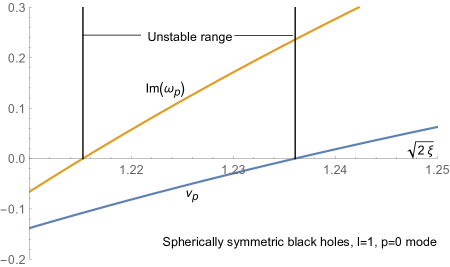
Figure 1: Frequency $\omega_{p}$ and $\nu_{p}$ on the spherically symmetric black hole $\gamma=1$, for the non-minimally coupled scalar with non-minimal coupling $\xi$, on the mode with $p=0$ and angular momentum $l=1$. The allowed modes correspond to values of $\xi$ such that $\nu_{p}<0$. The modes with frequencies with positive imaginary part are unstable. In consequence, stability sets an upper bound on the value of the non-minimal coupling parameter.

We can see from equations (40) and (42) that for a massless, minimally coupled scalar, namely for $\xi=0$, it is not possible to fulfill the boundary conditions and there are no quasinormal modes of such massless scalar probe fields on the black hole background. This situation is similar to what occurs for a massless scalar probe on the asymptotically locally flat, static black holes in New Massive Gravity Anabalon:2019zae . In the present case, a non-vanishing value of the non-minimal coupling allows for non-trivial quasinormal modes, provided (40) and (42) are fulfilled. It is very interesting to notice that such quasinormal frequencies do not depend on the black hole mass $M=M(r_{+})$, and therefore all the black holes in the family (4) for different values of $r_{+}$ are isospectral in what regards the quasinormal modes of the non-minimally coupled scalars. Notice that this is the case both, in the spherically symmetric and planar cases recovered by setting $\gamma=1$ and $\gamma=0$, respectively.

It is also illuminating to rewrite the second order equation for the radial profile of the non-minimally coupled scalar probe in a Schroedinger-like form. This is achieved by introducing the tortoise coordinate $r_{\ast}$ for the metric (4)

$$r_{\ast}=\frac{1}{2\alpha}\ln\left(r^{2}-r_{+}^{2}\right)\rightarrow r=\sqrt{r_{+}^{2}+e^{2\alpha r_{\ast}}}\ ,$$ (43)

which maps $r\in]r_{+},\infty[$ to the whole real line, i.e. $r_{\ast}\in]-\infty,+\infty[$. Notice that we have been able to explicitly solve $r$ in terms of $r_{\ast}$, which is not possible for Schwarzschild black hole. Using this fact, we can obtain the potential of the Schroedinger-like equation explicitly in terms of $r_{\ast}$. Introducing

$$F\left(r\right)=\frac{H\left(r\right)}{r}\ ,$$ (44)

leads to

$$-\frac{d^{2}F}{dr_{\ast}^{2}}+U\left(r_{\ast}\right)F=\omega^{2}F\ ,$$ (45)

with

$$U\left(r_{\ast}\right)=\frac{\alpha\left[r_{+}^{2}\left(2\left(1-4\xi\right)\alpha+2\gamma\xi+k^{2}\right)e^{2\alpha r_{\ast}}+e^{4\alpha r_{\ast}}\left(\left(1-6\xi\right)\alpha+2\gamma\xi+k^{2}\right)\right]}{\left(r_{+}^{2}+e^{2\alpha r_{\ast}}\right)^{2}}\ .$$ (46)

Notice that this potential always vanishes in the near horizon region, namely when $r_{\ast}\rightarrow-\infty$. Even more, when $\xi=0$ as $r_{\ast}\rightarrow\infty$ the potential approaches a positive constant and has a Heviside-like shape, being a monotonically increasing function of $r_{\ast}$. As mentioned above, for the minimally coupled case it is impossible to find quasinormal modes, which is consistent with the basic fact that Schroedinger equation on a Heviside potential cannot have solutions that approach zero at $x\rightarrow\infty$ and that represent purely “outgoing” modes travelling towards the left as $x\rightarrow-\infty$.

In what follows we move to the problem of computing the spectrum for a non-minimally coupled scalar probe on the gravitational solitons recently constructed in Canfora:2021nca in $\mathcal{N}=4$ $SU\left(2\right)\times SU\left(2\right)$ gauged supergravity, both in the supersymmetric and non-supersymmetric cases.

III Spectrum of probe scalars on solitons

As shown in Canfora:2021nca , $\mathcal{N}=4$ $SU(2)\times SU\left(2\right)$ gauged supergravity has the following soliton solution

$$ds^{2}=-\rho dt^{2}+g\left(\rho\right)d\varphi^{2}+\frac{d\rho^{2}}{g\left(\rho\right)}+\rho dy^{2}\ ,$$ (47)

where

$$g\left(\rho\right)=\alpha\left(\rho-m-\frac{q^{2}}{\rho}\right)\ ,$$ (48)

$m$ and $q$ being integration constants, $\alpha$ is related with the gauge couplings and $\varphi$ is identified with period $\beta_{\varphi}$ given by

$$\beta_{\varphi}=\frac{4\pi}{g^{\prime}\left(\rho_{0}\right)}\ .$$ (49)

Here $g\left(\rho_{0}\right)=0$, $\rho\geq\rho_{0}$ and the constants $\alpha$, $q$, the gauge fields and the dilaton are given by

$$\alpha =\frac{1}{2}\left(e_{A}^{2}+e_{B}^{2}\right)\ ,\qquad q^{2}=\frac{8\left(Q_{A}^{2}+Q_{B}^{2}\right)}{e_{A}^{2}+e_{B}^{2}}\ ,$$ (50)

$$A_{\left[1\right]}^{i} =\frac{Q_{A}}{\rho}d\varphi\delta_{3}^{i}\ ,\qquad\,\quad B_{\left[1\right]}^{i}=\frac{Q_{B}}{\rho}d\varphi\delta_{3}^{i}\ ,$$ (51)

$$\phi\left(r\right) =-\frac{1}{2}\ln\rho\ .$$ (52)

For general values of the integration constants $m$ and $q$, the non-minimally coupled scalar probe does not admit a solution in a closed form. Nevertheless, for the case $q=0$ and $m$ arbitrary, as well as for the case $m=0$ and $q$ arbitrary, the non-minimally coupled scalar field can indeed be solved in terms of hypergeometric functions, consequently boundary conditions can be imposed in a closed manner, leading to a discrete set of frequencies. Hereafter we refer to these special cases as soliton-1 and soliton-2, which are defined by the metric (47), with $g\left(\rho\right)$ given by

$$g_{sol1}\left(\rho\right) =\alpha\left(\rho-m\right)\ ,$$ (53)

$$g_{sol2}\left(\rho\right) =\alpha\left(\rho-\frac{q^{2}}{\rho}\right)\ ,$$ (54)

respectively.The soliton-2 spacetime leads to a supersymmetric configuration that preserves 1/4 of the supersymmetry Canfora:2021nca .

Defining $\varphi=\frac{\beta_{\varphi}}{2\pi}\phi$, the coordinate $\phi$ will have period $2\pi$, and the metric (47) reduces to

$$ds^{2}=-\rho dt^{2}+\frac{\beta_{\varphi}^{2}}{4\pi^{2}}g\left(\rho\right)d\phi^{2}+\frac{d\rho^{2}}{g\left(\rho\right)}+\rho dy^{2}\ .$$ (55)

Given the isometries of this spacetime we write the following separation ansatz for a scalar probe

$$\Phi=\operatorname{Re}\left(\sum_{n}\int d\omega dke^{-i\omega t+iky+in\phi}H_{\omega,k,n}\left(\rho\right)\right)\ .$$ (56)

The Ricci scalar of (55) has a non-trivial profile and it is given by

$$R=\frac{g\left(\rho\right)}{2\rho^{2}}-g^{\prime\prime}\left(\rho\right)-\frac{2g^{\prime}\left(\rho\right)}{\rho}\ .$$ (57)

Introducing the notation $H_{\omega,k,n}\left(\rho\right)=H\left(\rho\right)$, the equation for the non-minimally coupled scalar

$$\square\Phi-\xi R\Phi=0\ ,$$ (58)

leads to the following ODE for the radial dependence

$$2\rho^{2}g^{2}\beta_{\varphi}^{2}H^{\prime\prime}+2g\rho\beta_{\varphi}^{2}\left(g\rho\right)^{\prime}H^{\prime}+\left(g\beta_{\varphi}^{2}\left(2g^{\prime\prime}\rho^{2}+4g^{\prime}\rho-g\right)\xi-2\rho\left(4\pi^{2}n^{2}\rho+g\beta_{\varphi}^{2}\left(k^{2}-\omega^{2}\right)\right)\right)H=0\ .$$ (59)

Here the prime denotes derivative with respect to $\rho$. In what follows we analyze this equation for both soliton-1 and soliton-2 spacetimes, separately.

III.1 Non-supersymmetric soliton

For the family of solitons defined by the function soliton-1 in (53), we have $\rho_{0}=m$, and $g^{\prime}\left(\rho_{0}\right)=\alpha$, therefore $\beta_{\varphi}=\frac{4\pi}{\alpha}$. Introducing the coordinate $x$ such that

$$\rho=\frac{\rho_{0}}{1-x}\ ,$$ (60)

which maps $\rho\in[\rho_{0},\infty[$ to $x\in[0,1[$, leads to an equation for the radial profile that can be integrated in terms of hypergeometric functions. Imposing regularity at the origin $\rho=\rho_{0}$ ($x=0$) leads to the following solution

$$H\left(\rho\left(x\right)\right)=C_{1}x^{\frac{|n|}{2}}\left(1-x\right)^{\frac{1}{2}\left(1-\sqrt{\left(1-6\xi\right)+n^{2}+\frac{4\left(k^{2}-\omega^{2}\right)}{\alpha}}\right)}F\left(\alpha_{1},\beta_{1},\gamma_{1},x\right)\ ,$$ (61)

with

$$\alpha_{1} =\frac{1}{2}\left(1+|n|+\sqrt{2\xi}\right)-\frac{1}{2}\sqrt{(1-6\xi+n^{2})+\frac{4\left(k^{2}-\omega^{2}\right)}{\alpha}}\ ,$$ (62)

$$\beta_{1} =\frac{1}{2}\left(1+|n|-\sqrt{2\xi}\right)-\frac{1}{2}\sqrt{(1-6\xi+n^{2})+\frac{4\left(k^{2}-\omega^{2}\right)}{\alpha}}\ ,$$ (63)

$$\gamma_{1} =1+|n|\ .$$

As in the previous section, using Kummer identities allows to rewrite (61) as

$$H\left(\rho\left(x\right)\right) =C_{1}x^{\frac{|n|}{2}}\left(1-x\right)^{\frac{1}{2}\left(1-\sqrt{\left(1-6\xi\right)+n^{2}+\frac{4\left(k^{2}-\omega^{2}\right)}{\alpha}}\right)}\times$$

$$\left[\frac{\Gamma\left(\gamma_{1}\right)\Gamma\left(\gamma_{1}-\alpha_{1}-\beta_{1}\right)}{\Gamma\left(\gamma_{1}-\alpha_{1}\right)\Gamma\left(\gamma_{1}-\beta_{1}\right)}F\left(\alpha_{1},\beta_{1},\alpha_{1}+\beta_{1}+1-\gamma_{1},1-x\right)\right.$$ (64)

$$\left.+\left(1-x\right)^{\gamma_{1}-\alpha_{1}-\beta_{1}}\frac{\Gamma\left(\gamma_{1}\right)\Gamma\left(\alpha_{1}+\beta_{1}-\gamma_{1}\right)}{\Gamma\left(\alpha_{1}\right)\Gamma\left(\beta_{1}\right)}F\left(\gamma_{1}-\alpha_{1},\gamma_{1}-\beta_{1},1+\gamma_{1}-\alpha_{1}-\beta_{1},1-x\right)\right]$$ (65)

which leads to the following two leading terms on each branch of the asymptotic behavior as $x\rightarrow 1$

$$H\left(x\right)\underset{x\rightarrow 1}{\sim}A_{1}\left(1-x\right)^{\delta_{-}}+B_{1}\left(1-x\right)^{\delta+}\ ,$$ (66)

with

$$\delta_{\pm}=\frac{1}{2}\left(1\pm\sqrt{\left(1-6\xi\right)+n^{2}+\frac{4\left(k^{2}-\omega^{2}\right)}{\alpha}}\right)\ ,$$ (67)

and

$$A_{1} =\frac{\Gamma\left(\gamma_{1}\right)\Gamma\left(\gamma_{1}-\alpha_{1}-\beta_{1}\right)}{\Gamma\left(\gamma_{1}-\alpha_{1}\right)\Gamma\left(\gamma_{1}-\beta_{1}\right)}\ ,$$ (68)

$$B_{1} =\frac{\Gamma\left(\gamma_{1}\right)\Gamma\left(\alpha_{1}+\beta_{1}-\gamma_{1}\right)}{\Gamma\left(\alpha_{1}\right)\Gamma\left(\beta_{1}\right)}\ .$$ (69)

Since the exponents in the asymptotic behavior (66) are $\omega$ dependent, we must be careful when imposing the boundary conditions. Again, the boundary term coming from the on-shell variation of the action principle (34)-(35) leads to a single contribution at infinity coming from the surface $x=x_{0}\rightarrow 1$. In terms of the coordinate $x$, the non-supersymmetric soliton spacetime reads

$$ds^{2}=-\frac{\rho_{0}}{1-x}dt^{2}+\frac{4\rho_{0}x}{1-x}d\phi^{2}+\frac{\rho_{0}}{\alpha x\left(1-x\right)^{3}}dx^{2}+\frac{\rho_{0}}{1-x}dy^{2}\ ,$$ (70)

while the boundary term of the on-shell variation of the action reads

$$\lim_{r\rightarrow\infty}\int d^{3}x\sqrt{-\gamma}\hat{n}_{\mu}\nabla^{\mu}\Phi\delta\Phi$$

$$\sim\lim_{x\rightarrow 1}\left(\delta_{-}^{2}A_{1}^{2}\left(1-x\right)^{2\delta_{-}-1}+\delta_{+}^{2}B_{1}^{2}\left(1-x\right)^{2\delta_{+}-1}+A_{1}B_{1}\left(\delta_{+}+\delta_{-}\right)\left(1-x\right)^{\delta_{+}+\delta_{-}-1}\right)\delta C_{1}$$ (71)

It can be checked that $\operatorname{Re}\left(2\delta_{-}-1\right)<0$ on the whole complex $\omega$-plane, while $\operatorname{Re}\left(2\delta_{+}-1\right)>0$ and $\delta_{+}+\delta_{-}-1=0$. Therefore, in order to make the boundary term to vanish when evaluated on-shell on the branch that is regular at the origin, we must impose

$$A_{1}=\frac{\Gamma\left(\gamma_{1}\right)\Gamma\left(\gamma_{1}-\alpha_{1}-\beta_{1}\right)}{\Gamma\left(\gamma_{1}-\alpha_{1}\right)\Gamma\left(\gamma_{1}-\beta_{1}\right)}=0\ .$$ (72)

Notice that this is actually a Dirichlet boundary condition as can be seen from (66). The spectrum is therefore obtained from

$$\gamma_{1}-\alpha_{1} =\frac{\sqrt{(1-6\xi+n^{2})\alpha+4\left(k^{2}-\omega^{2}\right)}+\sqrt{\alpha}\left(1+|n|-\sqrt{2\xi}\right)}{2\sqrt{\alpha}}=-p\ ,$$ (73)

$$\gamma_{1}-\beta_{1} =\frac{\sqrt{(1-6\xi+n^{2})\alpha+4\left(k^{2}-\omega^{2}\right)}+\sqrt{\alpha}\left(1+|n|+\sqrt{2\xi}\right)}{2\sqrt{\alpha}}=-q\ ,$$ (74)

with $q$ and $p$ in $\left\{0,1,2,...\right\}$. One can also check that the second quantization condition (74) cannot be fulfilled, nevertheless the quantization condition (73) leads to the spectrum

$$\omega_{p}=\pm\frac{1}{2}\sqrt{2\alpha\left(|n|+2p+1\right)\sqrt{2\xi}+4k^{2}-2\left(|n|\left(1+2p\right)+4\xi+2p\left(1+p\right)\right)\alpha}\ ,$$ (75)

which is a valid solution of (73) provided

$$\nu_{ns}:=|n|+1-\sqrt{2\xi}+2p<0\ .$$ (76)

As in the case of the black hole, for the non-supersymmetric soliton requiring regularity at the origin and Dirichlet boundary condition at infinity leads to an eigenvalue problem with a void spectrum when $\xi=0$. Nevertheless, the presence of the non-minimal coupling leads to non-trivial probe modes.

The spectrum of the scalar on the non-supersymmetric soliton can be of diverse nature. Depending on the values of the parameters, it could be void, purely oscillatory namely with real frequencies (75) or unstable. The different behavior can be seen as separated by thresholds in the value of the non-minimal coupling $\xi$. Figure 2 shows two possible spectra.

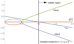
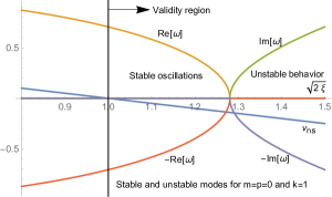
Figure 2: The panels show the spectra of stable and unstable modes of the non-minimally coupled scalar probe on the background of the non-supersymmetric soliton. Valid solutions for the quantization equation leading to the frequencies require $\nu_{p}<0$, therefore in both panels, to the left of the vertical black line, there are no allowed modes given our boundary conditions.

III.2 Supersymmetric soliton

The 1/4 supersymmetric soliton is given by the metric (55) with the function $g\left(\rho\right)$ given by

$$g_{sol2}\left(\rho\right)=\alpha\left(\rho-\frac{q^{2}}{\rho}\right)\ .$$ (77)

In this case the smooth origin of the spacetime is located at $\rho=\rho_{0}=q$ and the equation for the radial profile of the non-minimally coupled scalar probe has the following solution which is regular at the origin

$$H\left(x\right)=C_{1}x^{\frac{|n|}{2}}\left(1-x\right)^{\frac{1}{4}-\frac{1}{4}\sqrt{\left(1-6\xi\right)+4n^{2}+\frac{\left(k^{2}-4\omega^{2}\right)}{\alpha}}}F\left(\alpha_{2},\beta_{2},\gamma_{2},x\right)\ ,$$ (78)

where in this case the coordinate $x$ is conveniently chosen as

$$\rho=\frac{\rho_{0}}{\left(1-x\right)^{1/2}}\ .$$ (79)

Here, the parameters of the hypergeometric function in (78) are given by

$$\alpha_{2} =-\frac{1}{4}\sqrt{1-6\xi+4n^{2}+\frac{4\left(k^{2}-\omega^{2}\right)}{\alpha}}+\frac{1}{2}\left(|n|+1+\frac{1}{2}\sqrt{1+2\xi}\right)\ ,$$ (80)

$$\beta_{2} =-\frac{1}{4}\sqrt{1-6\xi+4n^{2}+\frac{4\left(k^{2}-\omega^{2}\right)}{\alpha}}+\frac{1}{2}\left(|n|+1-\frac{1}{2}\sqrt{1+2\xi}\right)\ ,$$ (81)

$$\gamma_{2} =1+|n|\ .$$ (82)

Using Kummer identity in (78) leads to the following leading terms of the two branches of asymptotic behavior

$$H\left(x\right)\sim_{x\rightarrow 1}A_{2}\left(1-x\right)^{\lambda_{-}}+B_{2}\left(1-x\right)^{\lambda_{+}}\ ,$$ (83)

with

$$\lambda_{\pm}=\frac{1}{4}\pm\frac{1}{4}\sqrt{\left(1-6\xi\right)+4n^{2}+\frac{\left(k^{2}-4\omega^{2}\right)}{\alpha}}\ ,$$ (84)

and

$$A_{2} =\frac{\Gamma\left(\gamma_{2}\right)\Gamma\left(\gamma_{2}-\alpha_{2}-\beta_{2}\right)}{\Gamma\left(\gamma_{2}-\alpha_{2}\right)\Gamma\left(\gamma_{2}-\beta_{2}\right)}\ ,$$

$$B_{2} =\frac{\Gamma\left(\gamma_{2}\right)\Gamma\left(\alpha_{2}+\beta_{2}-\gamma_{2}\right)}{\Gamma\left(\alpha_{2}\right)\Gamma\left(\beta_{2}\right)}\ .$$ (85)

As in the previous section, when the variation of the action is evaluated on the solution that is regular at the origin, one obtains a boundary term that vanishes iff

$$A_{2}=\frac{\Gamma\left(\gamma_{2}\right)\Gamma\left(\gamma_{2}-\alpha_{2}-\beta_{2}\right)}{\Gamma\left(\gamma_{2}-\alpha_{2}\right)\Gamma\left(\gamma_{2}-\beta_{2}\right)}=0\ .$$ (86)

In consequence, this implies the following two quantization conditions for the spectrum

$$\gamma_{2}-\alpha_{2} =\frac{1}{2}+\frac{|n|}{2}+\frac{1}{4}\sqrt{1-6\xi+4n^{2}+\frac{4\left(k^{2}-\omega^{2}\right)}{\alpha}}-\frac{1}{4}\sqrt{1+2\xi}=-p\ ,$$ (87)

$$\gamma_{2}-\beta_{2} =\frac{1}{2}+\frac{|n|}{2}+\frac{1}{4}\sqrt{1-6\xi+4n^{2}+\frac{4\left(k^{2}-\omega^{2}\right)}{\alpha}}+\frac{1}{4}\sqrt{1+2\xi}=-q\ ,$$ (88)

with $p$ and $q$ elements of $\left\{0,1,2,3,...\right\}$. It can be shown that the second condition cannot be fulfilled, while the former leads to the spectrum

$$\omega=\pm\sqrt{k^{2}+\left(1+|n|+2p\right)\alpha\sqrt{1+2\xi}-\alpha\left(2\xi+\left(1+2p\right)^{2}+2|n|\left(1+2p\right)\right)}\ ,$$ (89)

which are genuine solutions of (87) provided

$$\nu_{susy}=2+|n|+4p-\sqrt{1+2\xi}<0$$ (90)

Depending on the ranges of the parameters one can obtain the same qualitative spectra as in the non-supersymmetric soliton, namely there is a range of values for the non-minimal coupling for which the spectrum is void, while in the complementary range one can have both stable and unstable modes. Stable oscillatory behavior can be achieved provided one restricts the values of the non-minimal coupling.

IV Final remarks

In this paper we have found that $\mathcal{N}=4$ $SU\left(2\right)\times SU\left(2\right)$ gauged supergravity admits black holes an solitons with sufficiently simple geometry that allows to compute the spectrum of a non-minimal scalar probe in an exact manner. The spacetimes approach a background at infinity which is not maximally symmetric, but possesses and extra conformal Killing vector, which is due to the fact that the dilatonic potential of the theory does not have local extrema. As reported in Canfora:2021nca the solitonic geometries are smooth at the origin and can preserve $1/4$ of the supersymmetries and can be obtained from the corresponding planar black holes via a double analytic continuation, as it is the case of the recently reported solitons in $\mathcal{N}=2$ gauged supergravity in four dimensions Anabalon:2021tua . At the origin and in the near horizon region, the boundary conditions are clear and are given by regularity and purely ingoing modes, respectively. Due to the non-trivial geometry at infinity, the behavior of the scalar probe in the asymptotic region is given by powers of the radial coordinate which depend on the frequencies. In order to select a consistent boundary condition at infinity we impose that the on-shell variation of the action functionals must vanish. This leads to a Dirichlet boundary condition and allows to write the spectra in a closed form. For the massless scalar probe it is impossible to fulfill these boundary conditions. For the black holes, this is consistent with the fact that the effective Schroedinger-like potential controlling the radial dependence of the scalar probe in terms of the tortoise coordinate, has a Heaviside function shape. Including a non-minimal coupling allows for a non-trivial spectrum which surprisingly, in the case of the black hole, does not depend on the value of the mass of the spacetime. Therefore all these geometries are isospectral in what regards to the non-minimally coupled wave operator. Given the integrability properties of this potential it will be interesting to compare our results with the recently reported potentials coming from a geometric approach to spectral theory in connection with $SU\left(2\right)$ Seiberg-Witten theory with fundamental hypermultiplets (see Section 2 of Aminov:2020yma ). Such potential are also given in terms of ratios of linear combinations of exponentials.

Stability of the modes is achieved for a certain range of non-minimal couplings, above which one finds modes that are exponentially growing in time, and that are in consequence unstable. The stable and unstable regimes are separated by solutions to the boundary eigenvalue problem which are time independent. These solutions have the same properties as the scalar clouds found in Hod:2012px which from the point of view of the fully backreacting theory are branching spacetimes to a new family of solutions (see e.g. Herdeiro:2014goa ).

We have been able to solve in a closed form the non-minimally coupled scalar probe on a family of black holes and solitons of the Freedman-Schwarz model, even in the case of 1/4-BPS geometries. Such scalar probe goes beyond the field content of the theory, and it would be interesting to see whether some of the exact results we have obtained here, are also present in the context of gravitational perturbation theory considering only the fields that lead to the supersymetric model even if one has to rely on numerical or perturbative methods. We expect to report along these lines in the near future.

References

• (1) B. P. Abbott et al. [LIGO Scientific and Virgo], Phys. Rev. Lett. 116 (2016) no.6, 061102 doi:10.1103/PhysRevLett.116.061102 [arXiv:1602.03837 [gr-qc]].
• (2) G. T. Horowitz and V. E. Hubeny, Phys. Rev. D 62 (2000), 024027 doi:10.1103/PhysRevD.62.024027 [arXiv:hep-th/9909056 [hep-th]].
• (3) D. Birmingham, I. Sachs and S. N. Solodukhin, Phys. Rev. Lett. 88 (2002), 151301 doi:10.1103/PhysRevLett.88.151301 [arXiv:hep-th/0112055 [hep-th]].
• (4) J. S. F. Chan and R. B. Mann, Phys. Rev. D 55 (1997), 7546-7562 doi:10.1103/PhysRevD.55.7546 [arXiv:gr-qc/9612026 [gr-qc]].
• (5) V. Cardoso and J. P. S. Lemos, Phys. Rev. D 63 (2001), 124015 doi:10.1103/PhysRevD.63.124015 [arXiv:gr-qc/0101052 [gr-qc]].
• (6) R. Aros, C. Martinez, R. Troncoso and J. Zanelli, Phys. Rev. D 67 (2003), 044014 doi:10.1103/PhysRevD.67.044014 [arXiv:hep-th/0211024 [hep-th]].
• (7) J. Oliva and R. Troncoso, Phys. Rev. D 82 (2010), 027502 doi:10.1103/PhysRevD.82.027502 [arXiv:1003.2256 [hep-th]].
• (8) A. Giacomini, G. Giribet, M. Leston, J. Oliva and S. Ray, Phys. Rev. D 85 (2012), 124001 doi:10.1103/PhysRevD.85.124001 [arXiv:1203.0582 [hep-th]].
• (9) M. Cvetic and G. W. Gibbons, Phys. Rev. D 89 (2014) no.6, 064057 doi:10.1103/PhysRevD.89.064057 [arXiv:1312.2250 [gr-qc]].
• (10) M. Cvetic, G. W. Gibbons and Z. H. Saleem, Phys. Rev. D 90 (2014) no.12, 124046 doi:10.1103/PhysRevD.90.124046 [arXiv:1401.0544 [hep-th]].
• (11) M. Catalán, E. Cisternas, P. A. González and Y. Vásquez, Astrophys. Space Sci. 361 (2016) no.6, 189 doi:10.1007/s10509-016-2764-6 [arXiv:1404.3172 [gr-qc]].
• (12) P. A. González and Y. Vásquez, Eur. Phys. J. C 74 (2014) no.7, 2969 doi:10.1140/epjc/s10052-014-2969-1 [arXiv:1404.5371 [gr-qc]].
• (13) R. Bécar, P. A. González, J. Saavedra and Y. Vásquez, Eur. Phys. J. C 75 (2015) no.2, 57 doi:10.1140/epjc/s10052-015-3292-1 [arXiv:1412.6200 [gr-qc]].
• (14) A. M. Ares de Parga-Regalado and A. López-Ortega, Gen. Rel. Grav. 50 (2018) no.9, 113 doi:10.1007/s10714-018-2437-6
• (15) A. Anabalón, O. Fierro, J. Figueroa and J. Oliva, Eur. Phys. J. C 79 (2019) no.3, 281 doi:10.1140/epjc/s10052-019-6748-x [arXiv:1901.00448 [hep-th]].
• (16) M. Chernicoff, G. Giribet, J. Oliva and R. Stuardo, Phys. Rev. D 102 (2020) no.8, 084017 doi:10.1103/PhysRevD.102.084017 [arXiv:2005.04084 [hep-th]].
• (17) D. Z. Freedman and J. H. Schwarz, Nucl. Phys. B 137 (1978), 333-339 doi:10.1016/0550-3213(78)90526-6
• (18) A. H. Chamseddine and M. S. Volkov, Phys. Rev. Lett. 79 (1997), 3343-3346 doi:10.1103/PhysRevLett.79.3343 [arXiv:hep-th/9707176 [hep-th]].
• (19) A. H. Chamseddine and M. S. Volkov, Phys. Rev. D 57 (1998), 6242-6254 doi:10.1103/PhysRevD.57.6242 [arXiv:hep-th/9711181 [hep-th]].
• (20) D. Klemm, Nucl. Phys. B 545 (1999), 461-478 doi:10.1016/S0550-3213(98)00866-9 [arXiv:hep-th/9810090 [hep-th]].
• (21) S. Hod, Phys. Rev. D 86 (2012), 104026 [erratum: Phys. Rev. D 86 (2012), 129902] doi:10.1103/PhysRevD.86.129902 [arXiv:1211.3202 [gr-qc]].
• (22) C. A. R. Herdeiro and E. Radu, Phys. Rev. Lett. 112 (2014), 221101 doi:10.1103/PhysRevLett.112.221101 [arXiv:1403.2757 [gr-qc]].
• (23) F. Canfora, J. Oliva and M. Oyarzo, [arXiv:2111.11915 [hep-th]].
• (24) A. Anabalon and S. F. Ross, JHEP 07 (2021), 015 doi:10.1007/JHEP07(2021)015 [arXiv:2104.14572 [hep-th]].
• (25) G. Aminov, A. Grassi and Y. Hatsuda, [arXiv:2006.06111 [hep-th]].