A rodent paradigm for studying perceptual decisions under asymmetric reward
Xiaoyue Zhu 1,2,4, Jeffrey C. Erlich1,2,3,4,5*
1 NYU-ECNU Institute of Brain and Cognitive Science at NYU Shanghai, China
2 NYU Shanghai, Shanghai, China
3 Shanghai Key Laboratory of Brain Functional Genomics (Ministry of Education), East China Normal University, Shanghai, China
4 Center for Neural Science, New York University, New York, NY, United States of America
5 Sainsbury Wellcome Centre for Neural Circuits and Behaviour, University College London, London, United Kingdom
* jerlich@nyu.edu
Abstract
Many real-life decisions involve both perceptual processes and weighing the consequences of different actions. However, the neural mechanisms underlying perceptual decisions have typically been examined separately from those underlying economic decisions. Here, we trained rats to make choices informed by both perceptual and value cues on a trial-by-trial basis. As in typical perceptual tasks, subjects were rewarded for correctly categorizing a tone relative to a learned threshold. To add an economic component, a light indicated, on each trial, whether correct responses to one side gave higher rewards than correct responses to the other side. As such, on trials with some perceptual uncertainty, it could be worthwhile to choose the unlikely option, if it had higher expected value. We found that, despite subjects sensitivity to the frequency of the cue and the reward sizes, their behavior was not optimal: subjects tended to shift their choices in a stimulus-independent way following light flashes. Moreover, subjects tended to under-shift, which could be interpreted as being over-confident in their perceptual beliefs or as being risk-averse.
Introduction
We are often required to make decisions based on noisy perceptual evidence where the costs associated with one choice are quite different than the costs associated with the other choice. Consider a dramatic example: a radiologist who needs to detect the presence (or absence) of a malignant tumor from a CT scan. The judgment itself should only be based on perceptual information, such as the density, shape and curvature of the anomalous cluster. However, the cost of mistakes in these medical decisions are highly asymmetric. If the tumor is present and the doctor says ‘no’ (miss), the patient will be discharged and possibly die from the lack of treatment. On the other hand, if the tumor is absent and the doctor says ‘yes’ (false alarm), the patient will just go through more tests until the determination of cancer is clear. When a perceptual judgment incurs asymmetric outcomes, the decision maker must integrate both the strength of sensory evidence and the distinct costs of mistakes, or different benefits of actions. In fact, such decisions are commonplace in the real-life, from judging if the yogurt has gone bad to an animal judging whether the noise is caused by a predator or a prey.
Laboratory tasks studying the cognitive and neural mechanisms of decision under noisy sensory information typically assign equal reward to the options, where the subject is rewarded for categorizing the stimulus correctly. Recently, there is an emerging interest in studying perceptual decisions with asymmetric costs and reward, predominantly in humans (Diederich and Busemeyer, 2006; Diederich, 2008; Summerfield and Koechlin, 2010; Gao et al., 2011; Mulder et al., 2012) and non-human primates (Feng et al., 2009; Rorie et al., 2010). Despite the differences in tasks and models used, all of these experiments investigated how value information was integrated with sensory information during the decision process. One plausible mechanism is that the value information affects the processing of sensory information, such as by directly modulating the activity in primary sensory areas. Stănişor et al. (2013) found reward value is a good predictor of monkey V1 activity in a curve-tracing task, likely mediated by the top-down control of attention. Similar evidence was found in human V1, whose activity was modulated by reward value even in the absence of an overt saccade (Serences, 2008).
On the other hand, value information can also influence perceptual choices by adjusting the starting or ending point of the decision process. Evidence for this view came from studies using variants of the drift diffusion model (DDM), which depicts the decision mechanism as a ‘diffusion’ process, where the decision variable ‘drifts’ towards a threshold based on upcoming sensory information (Ratcliff, 1978). Naturally, the model’s way to reflect an asymmetric starting point (as a result of value) would be to change the starting position for the decision variable. Such model-based analysis has shown that a shift in the starting position of DDM can best explain behavior in human subjects (Summerfield and Koechlin, 2010; Gao et al., 2011; Mulder et al., 2012) and non-human primates (Rorie et al., 2010).
These two alternative hypotheses, that value information exerts influence on or separate from sensory processing, predict that asymmetric reward should lead to differential neural activity in the sensory or secondary motor areas, respectively. Moreover, causal evidence for either hypothesis can be obtained by inactivating the candidate areas during the stimulus presentation or choice phase. Th rat is an excellent model organism for studying the neurobiology of decision-making. Not only it is cost-effective, it also allows for manipulations with high temporal and spatial precision that are otherwise difficult in primates (e.g. Deisseroth, 2014; Kramer et al., 2013). Numerous groups have demonstrated that rats can learn complex perceptual and economic decision-making tasks, guided by visual and auditory cues (Constantinople et al., 2019; Miller et al., 2017; Erlich et al., 2015; Zhu et al., 2021). Lak et al. (2020) trained mice on a task where they detected visual gratings with varying contrast, shown on the left or right monitor. The reward was asymmetric such that in alternating blocks, reporting one side correctly entailed a larger reward than the other side. To maximize reward, the animals must integrate reward history with trial-by-trial visual cues. This is the first rodent task, as far as we are aware of, that investigates percept-value integration in a decision-making context. However, as the reward structure was not explicitly cued on each trial, this task is better suited for studying the learning of action-values than percept-value integration (Behrens et al., 2007). It is difficult to know exactly when in the trial the integration may be happening. Thus, we set out to develop a rodent task where the subject’s choice is guided by both the perceptual and value-based components on a trial-by-trial basis.
Materials and Methods
Subjects
Data from 7 male rats (4 Brown Norway, 3 Sprague Dawley; Vital River, Beijing, China) is included in this study. The animals were placed on a controlled-water schedule and had access to free water 20 minutes each day in addition to the water they earned in the task. They were kept on a reversed 12 hour light–dark cycle and were trained during their dark cycle. Animal use procedures were approved by New York University Shanghai International Animal Care and Use Committee following both U.S. and Chinese regulations.
Behavioral Apparatus
Animal training took place in custom behavioral chambers, located inside sound- and light-attenuated boxes. Each chamber (23 x 23 x 23 cm) was fitted with 8 nose ports arranged in four rows (Figure 3A), with a pair of speakers on the left and right side. Each nose port contained a pair of blue and yellow light emitting diodes (LED) for delivering visual stimuli, as well as an infrared LED and infrared phototransistor for detecting rats’ interactions with the port. The port in the bottom row contained a stainless steel tube for delivering water reward. Animals were loaded and unloaded from the behavioral chambers by technicians daily on a fixed schedule. Each training session lasted for 90 minutes.
The perceptual gambling task
Trials began with both yellow and blue light-emitting diodes (LED) turning on in the center port. This cued the animal to poke its nose into the center port and hold it there for 1 s – the ‘fixation’ period. As soon as the animal started fixation, a 500 ms tone would play from both speakers. The tone’s frequency (in space) was sampled from a Gaussian distribution centered at 3 and truncated at 2 and 4, values corresponding to 8 kHz, 4 kHz and 16 kHz. Unless otherwise specified, we will use the value throughout this manuscript. Specifically, the probability density function, , describing the distribution of tone frequencies was:
| (1) |
where is the standard deviation and controls the difficulty of the perceptual task; it was tuned for each animal. The boundaries where is truncated are defined by and . The perceptual task required subjects to report whether the of the tone was greater or less than 3. We counterbalanced the left / right assignment across animals, that animals with even subject ID were rewarded for tones on the left, and animals with odd ID were rewarded for tones on the right. We refer the correct port for frequencies lower than 3 as the ‘low port’, and the correct port for frequencies higher than 3 as the ‘high port’. After 1 s fixation, the animal was free to withdraw from the center port and poke into the left or right choice port. The animal was rewarded with the base amount if it chose correctly, no reward was delivered otherwise. If a trial had no flash and the animal was rewarded the base amount for choosing the correct port, we refer to these trials as ‘perceptual trials’. Around 30% to 65% of the total trials in a session were perceptual trials, the proportion was different for each animal (, mean and 95% C.I.).
On some trials, concurrent with the tone, the three ports of one side would flash their yellow LEDs in the rate of 10 Hz, lasting for the entire duration of fixation. The selection of the flashing side was independent of the correct side indicated by tone frequency. If the flashing side coincided with the correct side, the animal would be rewarded with times of the if it chose the correct port. The reward multiplier was tuned for each animal. If the flashing side was different than the correct side, the animal was rewarded the base amount if it chose the correct port. No reward was delivered for choosing the incorrect port. We refer to these trials as ‘perceptual gambling (PG) trials’. Around 35% to 70% of the total trials in a session were PG trials (). The inter-trial intervals (ITI) were between 3 and 10 seconds. A trial was considered a violation if the animal failed to poke into central 300 s after trial start, or it did not make a choice 30 s after fixation. Violations were excluded from all analyses.
Training pipeline
Animal training took place in four distinct phases: the operant conditioning phase, the fixation phase, the perceptual phase and the perceptual gambling phase.
The operant conditioning phase
In the operant conditioning phase, naive rats became familiar with the training apparatus and learned to poke into the reward port when illuminated. Trials began with the illumination of reward port, and water reward was immediately delivered upon port entry. After the rats learned to poke in the reward port reliably, they proceeded to the next training stage where they had to first poke into an illuminated choice port (left or right, randomly interleaved) before the reward port was illuminated for reward. They graduated to the next phase if they correctly performed these trials at least 40% of the session.
The fixation phase
In the fixation phase, rats started by initiating the trial by poking into the center port. To facilitate initial learning, only two tones were presented (2 and 4) and the same tone was presented in blocks of 5 to 20 trials. The fixation duration started from 0 ms, and was increased by 5 ms every time the rat maintained fixation in the previous trial, otherwise it remained unchanged. Rats graduated to the next phase once the fixation time reached 1 s and they could reliably choose the correct port given the frequency (75% correct rate overall).
The perceptual phase
The goal of the perceptual phase was to train the animals on the complete range of tone frequencies. Rats started with only 2 frequencies per side ([2, 2.25] and [3.75, 4]) in blocks of 5 to 20 trials. Once they showed sensitivity () to the existing tones based on a generalized linear model (GLM), more intermediate frequencies were added in pairs. The complete list of discrete frequencies was [2, 2.25, 2.5, 2.75, 3.25, 3.5, 3.75, 4], as they were spaced evenly apart in space. Once the performance was stable on all discrete frequencies, we introduced continuous frequencies by sampling from one of two truncated Gaussian distributions: and , while the correct port was the same in each block. Initially, was set to be large to expose the animals to a wide range of frequencies and made the task relatively easy. Once the animals displayed sharp psychometric curves with continuous stimuli in blocks, we removed the block structure and sampled from the full truncated Gaussian . The rats graduated from the perceptual phase if they showed sensitivity to the tones according to the GLM.
The perceptual gambling phase
Rats entered the final perceptual gambling phase with good understanding of the frequency-to-choice mapping. The goal of this phase was to let animals learn the meaning of the light flashes, which was introduced with a block structure. In a block of 20 to 30 trials, only one side would flash while the tone was still drawn from the truncated Gaussian distribution. In this phase, various task parameters were adapted to each animal’s reward sensitivity to induce the ‘perceptual gambling effect’. For example, if an animal did not shift its choice to the flashing side, we would increase to increase the expected value of the flashing side, decrease to make the trials more perceptually challenging and thus increase perceptual uncertainty, or increase the block length. The block length was gradually reduced to 1 - 3 once the subjects reliably shifted their choices in response to the flashing side.
Modeling with Bayesian decision theory
The perceptual gambling task is a binary classification task with asymmetric action costs. On each trial, the rat has to take an action that requires inferring the correct class of its auditory observation from the actual stimulus frequency . The probability of occurrence of each class is captured by the probability distribution , known as class priors. The distribution of the observation is specified conditioned on the class and denoted by , this is known as the likelihood. In our task, cannot be directly known but had to be derived from other conditional distributions, which will be described below. Together, the distributions and define a ‘generative model’, a Bayesian description of how the observations arise from the auditory stimulus presented on each trial (Ma, 2019). The main assumption of Bayesian modeling is that the rat has learned the distributions specified in the generative model, and it utilizes this knowledge fully when inferring possible states of the world. This is done by using Bayes’ rule,
| (2) |
where denotes the inferred posterior probability of a certain class given the stimulus frequency, and acts as a normalization factor. We describe our modeling process in three distinct steps: defining the generative model, computing the posterior distribution, and choosing an action to minimize cost (following Ma, 2019).
Defining the generative model
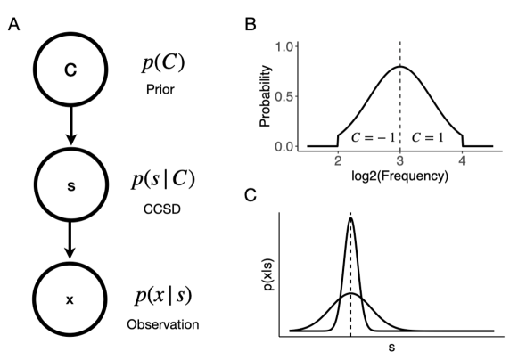
The generative model is shown in Figure 1A. It has three nodes: the correct class , the stimulus frequency , and the animal’s noisy observation . The rat’s goal was to correctly report , making that the world state of interest. can take on two possible values: 1 for the high port being correct, and -1 for the low port being correct. Associated with is a distribution , which is specified by two values, and . In our task, , as the correct class was determined by the frequency relative to 3 drawn from the symmetrical Gaussian distribution. The stimulus distribution is thus a class-conditioned stimulus distribution (CCSD), which is denoted by and for the two classes, respectively. As the stimulus , was drawn from the Gaussian and then designated to be , the two CCSDs are mirror-images of each other (Figure 1B). Formally,
| (3) | ||||
| (4) |
To complete the generative model, we need to define how the animals made observations based on the actual stimulus, . Conventionally, the observation, , is defined as a normal distribution centered at with standard deviation , which denotes the perceptual noise of the animal.
| (5) |
Computing the posterior distribution
Computing the posterior distribution involves both the class likelihood and class prior . The question is now how we can write the class likelihood in terms of the distributions specified in the generative model above. As observation is only dependent on , the class likelihood can be obtained by marginalizing over the intermediate variable :
| (6) | ||||
| (7) |
We can now write the posterior distribution as follows, where all the distributions have been specified:
| (8) | ||||
| (9) |
Choosing an action to minimize cost
If the task were just a perceptual task where the animals were rewarded equally for reporting the correct class, the optimal Bayesian decision maker should compare the two class posteriors and report the class with higher probability:
| (10) |
where is the decision variable and its sign indicates the chosen class. However, the key component of the perceptual gambling task was the asymmetric reward cued by flashing lights. According to BDT, the animal’s decision should consider the uneven ‘cost’ of the actions and choose the one with minimal cost on each trial. We define the cost function as , denoting the cost (loss of reward) of action when the correct class is and the flashing condition is . Let denote flashes on the high side, for flashes on the low side, and denote no flashes at all. Further, let the base correct reward be and the reward multiplier be . Then the cost function of the action given the correct class and flashing side can be summarized in the following table:
| 0 | 0 | 0 | ||||
| 0 | 0 | 0 | ||||
For example, the action cost of reporting class 1 () when the true class is -1 () and the flashing side is also -1 () is , as the animal is ‘missing out’ on reward if it reported correctly. The action cost of reporting class 1 () when the true class is 1 () is 0 regardless of the flashing side, as it is the only action to be rewarded in this scenario. To incorporate the cost function into the decision variable, we assume the animal has a representation of the posterior-weighted cost for each action. Concretely, the posterior-weighted cost for choosing class 1 becomes
| (11) |
And for class -1 becomes
| (12) |
where is the exponent on the animal’s utility function. In our task, we only tested 2 costs, so we could have, instead of an exponent, included a multiplicative reward scaling parameter. However, this is a classic functional form for marginal utility, that allows us to interpret animals with as risk averse and animals with as risk seeking. Finally, the decision variable can be expressed as the log ratio between and :
| (13) | ||||
| (14) |
From the cost function table, we know that , thus becomes
| (15) | ||||
| (16) | ||||
| (17) |
Different from Equation (10), the sign of the decision variable takes on the opposite value of the final class of choice. The reversion is due to the fact that the goal is to minimize the action cost rather than maximize the posterior distribution. Finally, we converted the decision variable into a probability of choosing using a logistic function:
| (18) |
where refers to all the parameters in the model.
The three-agent model
We observed that several animals exhibited ‘lapses’: poor performance even on very easy stimuli (Pisupati et al., 2019). In order to account for this behavior, we developed a three-agent model that includes a ‘rational’ agent that outputs from the BDT model, and two stimulus-independent agents that either habitually choose the low or high port. The choice on each trial becomes a weighted outcome of the votes from three agents with their respective mixing weights , each implementing a different behavioral strategy. Formally,
| (19) | ||||
| (20) | ||||
| (21) |
The full model we used to fit animal behavior is thus a BDT-inspired hybrid model, we refer to it as the ‘mixture-BDT’ model. For notation simplicity, in the following sections we will use to denote .
Analysis
For all analyses, we excluded time out violation trials (where the subjects disengaged from the ports for more than 30 s during the trial). All analysis and statistics were computed in R (version 3.6.3, R Foundation for Statistical Computing, Vienna, Austria).
Generalized Linear (Mixed-Effects) Models
Generalized linear models (GLM) and generalized linear mixed-effects models (GLMM) were fit using the stats and lme4 R packages (Bates et al., 2015). To test whether the animals were sensitive to both tone frequency and flashing side, we specified a mixed-effects model where the probability of choosing the high port was a logistic function of , the flashing side and their interaction as fixed effects. The flashing side is a categorical variable with three levels: low side flash, high side flash and no flash. The rat and an interaction of rat, and the flashing side are modeled as within-subject random effects. In standard R formula syntax:
| (22) |
where is 1 if the high port was chosen and 0 if the low port was chosen; is the subject ID for each rat.
To test whether an individual animal was sensitive to tone frequency and flashing side with each and combination, we specified a GLM as follows:
| (23) |
Only the and combination that resulted in a significant main effect of was included in this study (see Table 2).
To test whether the outcome of the previous trial affected choice on the current trial, we first classified the previous trial’s outcome into four categories: the animal chose the low port and was rewarded, the animal chose the low port and was unrewarded, the animal chose the high port and was rewarded, and the animal chose the high port and was unrewarded. A GLMM was specified:
| (24) |
where is a categorical variable with four levels as described above.
To test whether the animal has a tendency to repeat its previous choice, we specified a GLMM as follows:
| (25) |
where is 1 if the high port was chosen on the previous trial and 0 if the low port was chosen.
Trial difficulty analysis
To understand how perceptual difficulty affected the animal’s shift towards the flashing side, we employed a model-based analysis. First, we obtained the animal’s perceptual sensitivity using the aforementioned mixture-BDT model. Then, we computed Z-score for each tone frequency presented to this animal using the formula: . Based on the Z-score, the middle 33% trials () are labeled as ‘Hard’ trials, the 16.5% left and right to the hard trials are labeled as ‘Medium’ trials (; ), and the 16.5% left and right to the medium trials are labeled as ‘Easy’ trials (; ). By dividing trials this way, we ensured equal proportions of easy, medium and hard trials while taking into account the animal’s perceptual sensitivity. After computing the absolute change in percentage choosing the high port induced by light flashes for each difficulty condition, we performed a linear mixed-effects model (LMM) to test significance:
| (26) |
where refers to the absolute change.
Model fitting
Following modern statistical convention, we estimated the posterior distribution over model parameters with weakly informative priors using the rstan package (v2.21.2; Stan Development Team, 2020). rstan is the R interface of Stan (Stan Development Team, 2020), a probabilistic programming language that implements Hamiltonian Monte Carlo (HMC) algorithm for Bayesian inference. The prior over the utility exponent was , a weakly informative prior that prefers to be to risk-neutral. The prior over perceptual noise was , a reasonable range in space. The prior over the mixing weights was a Dirichlet distribution with the concentration parameter . The resulting distribution was broad and had the mean of 0.6, both and distribution had the mean of 0.2. By attributing more weight to the rational agent over the habitual agents, the prior reflected our selection of the experimental animals - only animals whose choices depended on the auditory cue were included. Four Markov chains with 1000 samples each were obtained for each model parameter after 1000 warm-up samples. The convergence diagnostic for each parameter was close to 1, indicating the chains mixed well.
Sigmoid function
The four-parameter sigmoid function was specified as follows:
| (27) |
where x is the tone frequency in , y is the probability choosing high port, and the four parameters are: , the inflection point of the sigmoid, controlling horizontal shifts; , the slope of the sigmoid; , the total lapse rate, and , representing the fraction of lapses that are low to high lapses. The sigmoid model was fit individually to each flash condition in each subject’s dataset using Stan.
Synthetic datasets
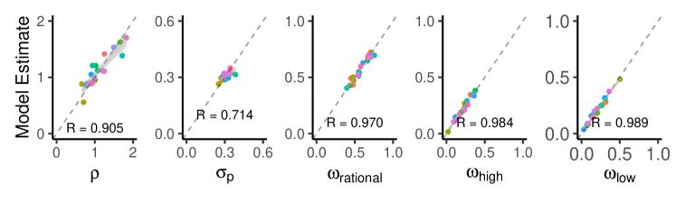
To test the validity of the mixture-BDT model, we first created synthetic datasets with parameters generated from the prior distributions described above. The model was used to fit on the synthetic datasets, and was able to recover the generative parameters accurately (Figure S1). This assured that the model had no systematic bias in estimating the parameters.
Model prediction confidence intervals
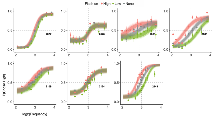
To estimate the confidence intervals with model prediction as in Figure 5A, we first generated a synthetic dataset with regularly spaced sound frequencies (incremented by 0.01). After parameter sampling in each iteration (in the generated quantities block), the sampled parameters were used to predict the choices given the synthetic offers. The resulting output is a n_iter n_sound matrix, where n_iter is the number of iterations and n_sound is the length of unique stimulus frequencies. Finally, , and confidence intervals for each offer were estimated by taking the respective quantiles of the n_iter predicted choices.
Mixture-BDT optimality analysis
To understand the relationship between and in obtaining maximum possible reward, we first created a synthetic task dataset with 1000 trials. The tone frequency was drawn from a truncated Gaussian centered at 3 and a standard deviation of 0.6. The was set to 5. There were equal proportions of the high flash, low flash and no flash trials (). We then created a mixture-BDT agent that is fully rational (). A grid search was performed to find the total reward for each combination of (0 to 1.5, incremented by 0.1) and (0 to 0.5, incremented by 0.1). The total reward () was computed as follows:
| (28) |
where is the probability of choosing the high port from the mixture-BDT agent on the i-th trial, is the reward delivered if choosing the low port on the i-th trial, and is the reward delivered if choosing the high port.
Code availability
The perceptual gambling dataset from the 7 animals and all the code used for analyses are freely available online at https://github.com/erlichlab/perceptual-gambling
Results
The perceptual gambling task
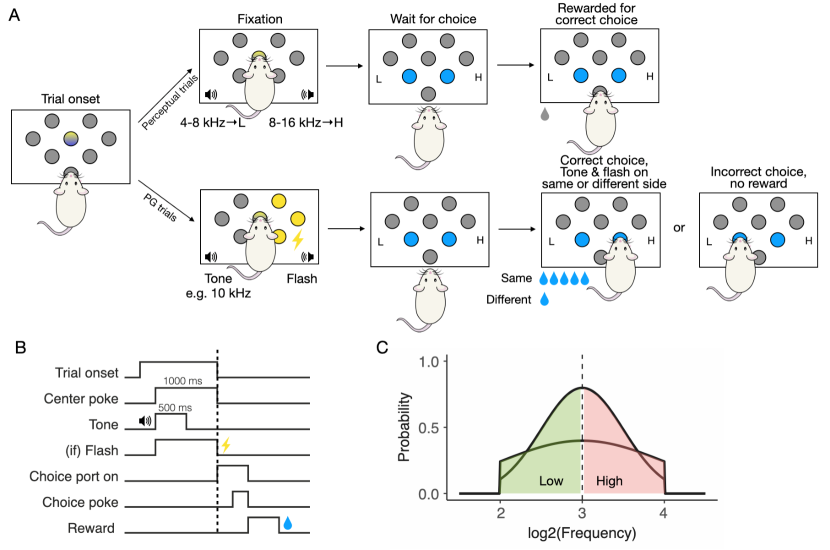
To establish a rodent framework to study decisions guided by both perceptual and value cues, we developed the perceptual gambling task. It was named so because although the correct decision was only informed by the perceptual cue, a reward-maximizing subject would choose the side with larger reward when the perceptual evidence was weak, effectively ‘gambling’ for more reward (Figure 2A). For example, imagine the subject was 75% certain that the stimulus should be categorized as ‘high’. But, on this trial, the subject knew that a correct ‘high’ response would be rewarded with 1 drop of water, while a correct ‘low’ response would fetch 8 drops. Then, the expected value of responding high would be . The expected value of responding low would be . As such, the task invites the animal to gamble based on its perceptual confidence, which was experimentally varied by requiring subjects to make easy and difficult perceptual decisions, and the values of the two responses.
Subjects were first trained on the pure perceptual version of the task with symmetric rewards, and we refer to these trials as ‘perceptual’ trials. On each trial, after self-initiation by poking into the center port, subjects fixated for 1 s while a tone would play from both speakers. Its frequency relative to 8 kHz indicated whether the left or right port was correct (counter-balanced across animals). We refer the correct port for frequencies lower than 8 kHz as ‘low port’, and the correct port for frequencies higher than 8 kHz as ‘high port’. The tone frequency (in space) was drawn from a truncated Gaussian distribution , where is the standard deviation and controls the difficulty of the perceptual task. The smaller is, the more concentrated the auditory stimulus is around the decision boundary, and the more perceptually challenging the trials will be (Figure 2C). Once the animals showed good performance on the perceptual trials, we introduced the value cues during fixation by flashing the yellow LEDs of the three left or right ports (Figure 2A). The choice of the flashing side was independent of the tone frequency. We delivered the perceptual and value cues through the auditory and visual modality, respectively, to avoid any effects from intra-modality attention. For example, a louder tone from one side might interact with the animal’s judgment of its frequency. If the correct port was on the same side as the flashing ports, correct responses resulted in a large reward (base reward ). Alternatively, if the flashing side was on the incorrect side, the animal was only rewarded the base amount for choosing the correct port. These trials are referred as ‘perceptual gambling (PG)’ trials. The perceptual trials were randomly interleaved with PG trials in a session, the ratio of the two trial types was different for each animal.
Training of the task was difficult, as the animal’s performance was highly sensitive to the values of task parameters, especially the difficulty of the perceptual task () and reward asymmetry (). This is not surprising, Kepecs et al. (2008) trained rats on an odor discrimination task and the animals were only rewarded (nor not) after a variable delay. While it was waiting for the reward, the rat had an option to ‘re-initiate’ the trial by leaving the choice port and start again, the frequency of which should correlate with its confidence of the perceptual decision. It was later reported that the training was also very parameter-sensitive, as the reward delay interacted with the rat’s temporal discounting function, similar to how the perceptual difficulty interacted with the reward sensitivity in our task (Kepecs and Mainen, 2012). Nonetheless, we successfully trained 7 animals on the task (see Table 2 for the effective task parameters for each animal). These 7 subjects were sensitive to both the auditory cue and the flashes with at least one set of task parameters, quantified by a generalized linear model (GLM). When the flash was first introduced, the animals did not show any bias towards the flashing side. Thus, the shifts in choices caused by the flashes were induced by learning, rather bottom-up attention.
| 2077 | 2078 | 2083 | 2085 | 2109 | 2124 | 2143 | |
|---|---|---|---|---|---|---|---|
| 1 | 1 | 1 | 1 | 0.3 | 0.3 | 0.3 | |
| 5 | 5 | 5 | 5 | 25 | 20 | 15 |
Animal behavior
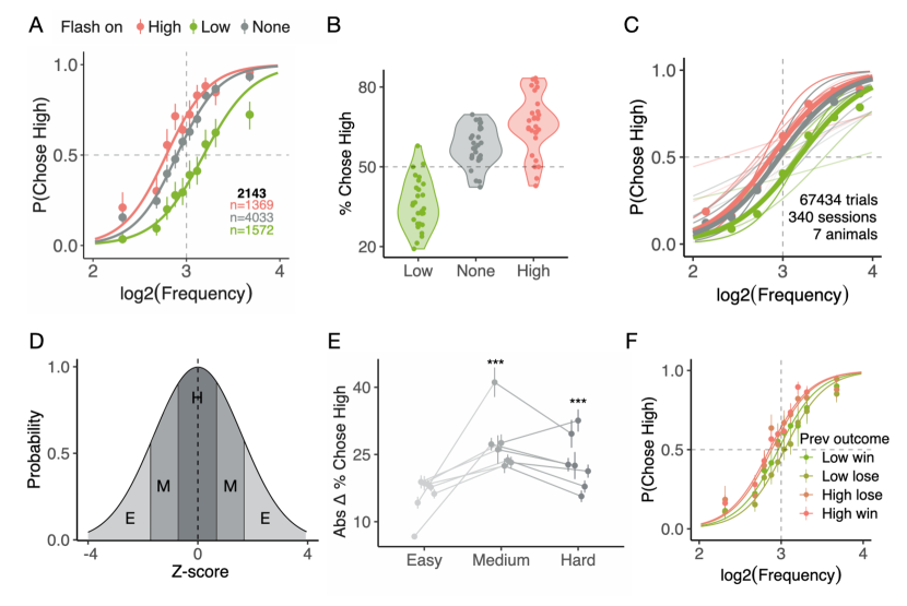
We trained 7 male rats (4 Brown Norway, 3 Sprague Dawley) on the perceptual gambling task. As expected, the animals’ performance was a function of evidence strength (see an example animal in Figure 3A; see population aggregates in Figure 3C). Moreover, the animals reliably shifted their choices towards the side with flashing lights (see example shift in Figure 3B, all animals in Figure S1). These effects were quantified using a generalized-linear mixed-effects model (GLMM). There was a significant main effect of tone frequency (), and a significant interaction between tone frequency and flash on the low side (). Interestingly, flashing on the high side did not affect behavior significantly on the group level ().
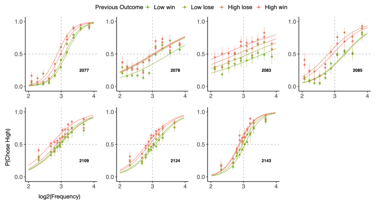
The premise of the task is that the animal should prefer the flashing side more when the stimulus is closer to the decision boundary. In other words, when perceptual evidence is weak, value information should have more influence on choice. To test whether this was true, we divided trials into easy, medium and hard trials based on their evidence strength relative to the animal’s perceptual noise, which was estimated using a Bayesian model (see description in the next section; Figure 3D). With a linear mixed-effects model (LMM), we found that trial difficulty significantly affected the absolute shift in percentage choosing the high port (; , Figure 3E). This is in line with our prediction that the subjects would shift more in medium and hard than easy trials, although the reason why they shifted more for medium than hard trials was unclear. Finally, we found that the choices on the current trial were significantly influenced by the outcome of the previous trial (GLMM, all ; see an example in Figure 3F, see all animals in Figure S2). Although the individual history effects differ, overall, the animals had a tendency to repeat its previous choice ().
A three-agent mixture model with Bayesian decision theory
While the GLMM results indicated that the animal’s choices were sensitive to both perceptual and value cues, it does not provide insight into the cognitive processes underlying task performance. To better understand how our animals integrated perceptual and value information, we developed a Bayesian decision theory (BDT) model (following Ma, 2019). Bayesian modeling starts with a generative model, specifying how the subject’s observation come about given the statistics of the environment, which is usually set by the experimenters. Using the Bayes’ rule, the subject then combines its prior with the observation to obtain the posterior, a probability distribution reflecting both the observed measurement and its prior belief. Finally, a Bayesian decision maker chooses an action in a principled manner by minimizing a cost function , which is determined by the state of the world and the action . The BDT framework is well suited for our task, as the animal acts by integrating a noisy perceptual stimulus (observation) and asymmetric reward associated with each choice (cost function).
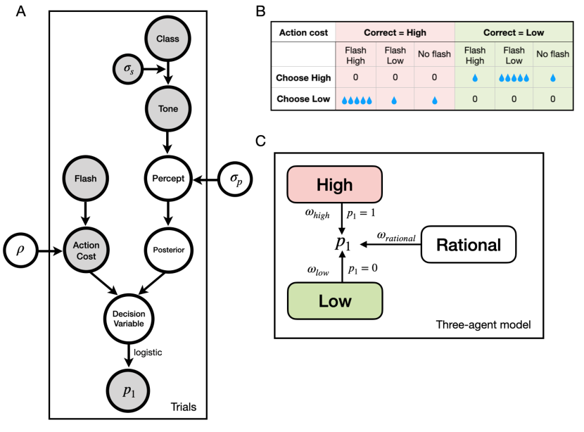
Next, we will briefly describe the model (Figure 4A, see modeling details in Methods). We start with the generative model, which specifies how the subject makes an observation given the stimulus frequency on each trial (Figure 1A). Recall that the stimulus was drawn from a truncated Gaussian centered at with standard deviation , which was set by the experimenter. Bayesian models assume that through experience, subjects learn this distribution, and utilize it when inferring the correct class (low or high) given the tone on each trial. Thus, the observation distribution is dependent on two parameters: , which is known, and as in , denoting the perceptual noise of each animal. The observation is then combined with class prior ( for each class) to compute the class posterior, representing the animal’s belief of each class given just the perceptual cue. To incorporate value information, we constructed a cost function where the choice is mapped to an action cost under different flash conditions (Figure 4B, Table 1). For example, when the high side is flashing and the correct class is high and the animal chooses low, the action cost would be , a miss of considerable size. We included an additional parameter as the exponent on the action cost, which is equivalent to the curvature of the animal’s utility function: , where denotes utility and is value. Finally, the -adjusted action cost of choosing each class is integrated with its class posterior as the decision variable (Equation (15)), which is transformed into a probability of choosing the high port using a logistic function.
We observed that some animals exhibited a constant, stimulus-independent rate of error known as ‘lapse’. Recently, it has been suggested to reflect exploration in a changing environment (Pisupati et al., 2019). To account for the lapses, we developed a ‘three-agent’ model that includes a ‘rational’ agent that outputs the probability of choosing the high port from the BDT model, a habitual ‘high’ agent that always chooses the high port, and a ‘low’ agent that always chooses the low port (Figure 4C). The choice on each trial is thus a weighted outcome of the votes from three agents with their respective mixing weights , each implementing a different behavioral strategy. We refer to the final hybrid model as the ‘mixture-BDT’ model.
The mixture-BDT model is insufficient to account for subjects’ behavior
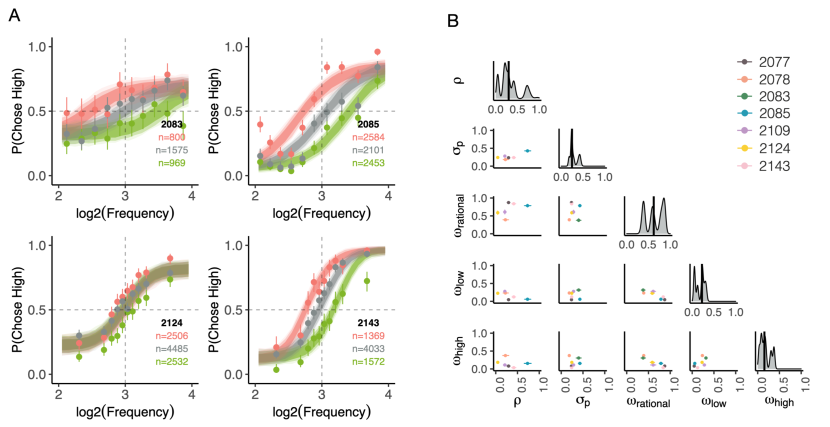
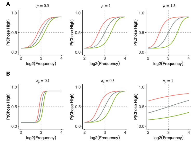
We first validated that the model can correctly recover generative parameters from synthetic data (Figure S1). We estimated the joint posterior over the parameters for each animal separately using Hamiltonian Monte Carlo sampling in Stan (see example animals in Figure 5A, see all animals in Figure S3). Details of the modeling, including the priors, can be found in the Methods section. Overall, the animals all had a concave utility function ( = 0.30 [0.04 1.39], median and 95% C.I. of concatenated posteriors across animals). They had medium to low levels of perceptual noise ( = 0.25 [0.17 0.45]), indicating that on average, they were sensitive to tone frequencies roughly 1.18 kHz apart. Consistent with GLMM results, animals with a sharper psychometric curve (e.g. 2143, pink dot in Figure 5B) had a smaller than animals with a flatter psychometric curve (e.g. 2083, green dot in Figure 5B). 2077, 2085 and 2143 were guided mostly by the rational agent ( = 0.84 [0.75 0.88], = 0.06 [0.04 0.14], = 0.08 [0.02 0.17], concatenated posteriors across these animals). In contrast, 2078, 2083, 2109 and 2124 displayed high levels of stimulus-independent bias ( = 0.49 [0.34 0.66], = 0.25 [0.21 0.34], = 0.24 [0.09 0.39]). However, this model failed to account for several aspect of animals’ behavior. First, there is only one parameter, , modulating how much subjects shift responses on PG trials, so the model predicts that the flash-induced shift should be symmetrical for left-flash and right-flash trials, which is not the case in our data. Second, the model predicts that flashes should result in horizontal shifts in the psychometric curve: the shift should depend on the perceptual uncertainty (Figure S4). In our data, some subjects shifted vertically (Figure 5A, 2124): a stimulus independent shift.
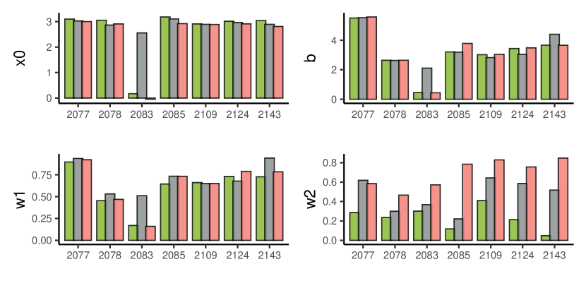
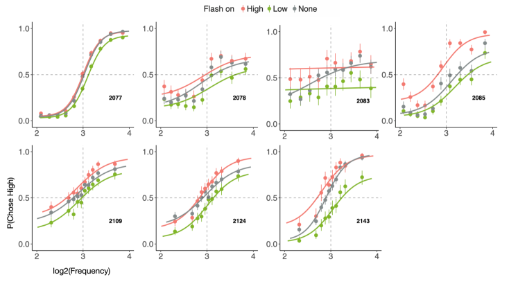
To quantify the degree to which the mixture-BDT model failed to fit the data, we refit the data, treating the perceptual trials, left flash and right flash trials as separate datasets, and fit each with a four-parameter sigmoid function (Equation (27), see details in Methods). If, as the mixture-BDT model predicts, flashes induces horizontal shifts (and small increases in slope), then the intercept term, , would change the most, with small changes in the slope, . However, in most animals, or changed in the flash trials relative to the perceptual trials, indicating vertical rather than horizontal shifts (Figure 6). Taken together, the modeling result suggests that the animal behavior is not well described by the normative BDT model, even after taking into account lapse, and thus the animals were not optimally integrating the cues.
The animals are not reward-maximizing
The vertical shifts induced by the flashes are sub-optimal. How much reward were the subjects missing out on? To answer this, we compared the rewards obtained by the animals with that by an optimal, reward-maximizing Bayesian decision-maker. We define ‘optimality’ here as obtaining the maximum possible reward given a fixed perceptual noise in a particular task dataset. Interestingly, it was found that in order for a purely rational BDT agent to obtain maximum reward, its utility curvature needs to balance with its perceptual noise (Figure 7A). This can be intuitively understood by going through some examples. For a subject with large , it will have a high error rate due to poor perceptual judgment, the strategy to maximize reward would be to choose the flashing side as much as possible and result in a convex utility function. Alternatively, a subject with very small will get most trials correct anyway, it does not need to ‘value’ the flash more than what it represents, resulting in a close-to-linear utility function. Another interesting result from the simulation analysis is that does not affect the total reward much when is small, but its value plays a big role when is large. This in part, explains why subjects like 2077 and 2143 are closest to the ‘optimal’, reward-maximizing agent even with smaller than the best (Figure 7B). For subjects 2078, 2109 and 2124, their large stimulus-independent bias seemed to be the culprit for obtaining lower reward overall. A fascinating example is 2083, its estimated and combination are close to being optimal (Figure 7A, green square). The fact that it only obtained 75% of the maximum reward was entirely due to its lapse rate, as a rational agent with its and obtained just as much reward as the optimal agent. On average, the animals obtained 83.2 3.3 % of the maximum reward obtained by their respective optimal agent, modeled with the same perceptual noise. Taken together, the analysis showed that the animals are not optimal in reward-maximization in the task, and this is due to a combination of high lapse rate and extreme risk-aversion.

Discussion
Decision-making is a term referring to the integration and transformation of external information with internal beliefs into an action. The external information may contain perceptual as well as value aspects of the decision required at hand. Despite its importance, only few studies have examined the behavioral and neurobiological underpinnings of decisions that involve percept-value integration. Here, we developed the perceptual gambling task where the rat made choices informed by both perceptual (tone frequency) and value (light flash) cues, on a trial-by-trial basis. Although the subjects did not, on average, shift their choices symmetrically by value as in monkeys (Rorie et al., 2010), the animals nevertheless showed sensitivity to flashes. We characterized behavior using the Bayesian decision theory, which assumes an optimal integration of individual perceptual noise and reward sensitivity, as well as the statistics of the task environment. It was found that the behavior was not well fit by the BDT model, even after accounting for lapses, because subjects responded to the flashes by shifting their choices in a stimulus independent way. Finally, we quantified the fraction of the reward that animals were foregoing by using a sub-optimal strategy. Model-based analysis revealed that the missing reward was due to a large lapse rates and risk aversion (extremely concave utility functions).
Overall, the results show that the animals are not behaving optimally in the task. Their choices were influenced by the previous trial’s outcome, even while the tone frequency and flash was independent across trials. Lak et al. (2020) also observed strong history effects, but in that task the animal was encouraged to incorporate history information due to the block design. Although Bayesian decision theory has had success in explaining and predicting human behavior (e.g. Cogley and Sargent, 2008; Körding and Wolpert, 2006), it has rarely been used to quantify rodent behavior. One key assumption of the Bayesian decision models is that the subject has learned the distributions of latent variables in the task environment and utilized them fully when making inference. It is likely that both the robust history effect and poor fit of the mixture-BDT are a result of incomplete or ongoing learning. For most animals, the training process involved adjusting perceptual difficulty and reward multiplier periodically to induce significant shifting. As a result, the animals may have internalized the environmental volatility and were actively exploring the reward contingencies. This may also underlie the substantial lapse rate observed in some animals (Pisupati et al., 2019). Thus, we emphasize that the poor performance of BDT does not suggest that our rats are non-Bayesian agents, it may merely reflect the lack of learning aspects in the theory. In fact, it seems that the monkey performance in a similar task from Rorie et al. (2010) can be well fit by the BDT, as their value-induced shift in the psychometric curves was horizontal.
The main takeaway from the training process was that task parameters like perceptual difficulty and reward multiplier heavily interacted with the animal’s sensory noise and utility exponent . Future researchers interested in adopting this framework are encouraged to use a model-based training method. Specifically, when is low and is small, to induce a behavioral shift, the experimenter needs to increase perceptual difficulty and increase the reward multiplier. When is high and is large, to prevent the animal from simply choosing the side with flash and ignoring the sound, the experimenter can reduce perceptual difficulty and decrease the reward multiplier. The animal’s can be estimated from the performance on the perceptual trials alone, prior to any value training. Estimating is challenging without training the animal on a task that exposes its subjective utility function. Nonetheless, results from choice under risk showed that most rats have concave utility functions ( ¡ 1, Zhu et al., 2021; Constantinople et al., 2019). On that account, it is reasonable to assume a small in the beginning of training unless the animal showed otherwise. However, we do not exclude the possibility that the animal may ‘adapt’ the shape of its utility function in different contexts, for example, a noisy perceptual decision-maker may deliberately become more risk-seeking to harvest more reward. There is some mixed evidence from behavioral ecology experiments supporting a context-dependent change in utility concavity (Kacelnik and El Mouden, 2013). Finally, given the small found in most animals in this study, it is advisable to use a narrower range of auditory stimuli (e.g. 5.65 - 11.31 kHz) to facilitate the training process.
In this manuscript, we did not explicitly test whether the flash-induced shift was due to a perceptual bias or a response bias, which predicts that the value information exerts influence on or separate from sensory processing, respectively. Nonetheless, the perceptual gambling task along with the mixture-BDT model together, can generate specific hypotheses on how to distinguish these two scenarios. Future researchers can record activity from the secondary motor regions and associative sensory regions in well-trained rats to establish correlative relationships. A response bias would predict increased activity in the motor region when the chosen side is cued for higher reward, whereas a perceptual bias would predict differential activity elicited by the same auditory stimulus in the sensory areas under flash and no-flash conditions. Furthermore, causal evidence for either scenario can be obtained with pharmacological and optogenetic inactivations. If by inactivating the secondary motor region the animal simply shifts less to the flashing side, which is equivalent to a decreased utility exponent in the model, the response bias hypothesis will be supported. Even more interestingly, this would suggest a dissociable process of perceptual decision and value computation. On the other hand, the perceptual bias will be supported if the animal shifts less by following inactivation of its associative sensory areas.
Another promising avenue of research enabled by the perceptual gambling task is the study of confidence. Confidence is generally defined as the degree of belief in the truth of a proposition or the reliability of a piece of information, be it memory, observation or decision (Kepecs and Mainen, 2012). One important nuance is that there confidence has to be about a specific belief. In the PG task, one can distinguish the perceptual confidence from the decision confidence. In signal detection theory, perceptual confidence is defined as the distance from an internal representation of a stimulus to the decision boundary. On average, accuracy is a proxy for perceptual confidence (Clarke et al., 1959; Galvin et al., 2003). This is a model of perceptual confidence, but it becomes indistinguishable from decision confidence in simple perceptual decision tasks. Recently, a Bayesian equivalent was proposed under the Bayesian decision theory, which defined confidence as the observer’s posterior probability of being correct (Kepecs and Mainen, 2012; Hangya et al., 2016; Pouget et al., 2016). Using the Bayesian definition of confidence, research groups were able to find behavioral and neural correlates that resemble the qualitative signatures of Bayesian confidence in rats (Kepecs et al., 2008; Lak et al., 2014) and humans (Sanders et al., 2016). We observe that the Bayesian decision theory framework can distinguish the two, such that the perceptual confidence is simply the log ratio of posterior sans action cost, and the decision confidence is the log ratio of posterior with action cost. Our task makes investigating the neural underpinnings of these two kinds of confidence possible. Specifically, areas computing perceptual confidence should not vary across flashing conditions, as the perceptual boundary remains the same (unless, of course, the change in value causes a change in percept). In contrast, areas responsible for decision confidence should show differential activities across conditions, as the asymmetric reward would shift the indifference point, entailing a considerable change in decision confidence even with the same perceptual stimulus. Activities in these areas can be related to the Bayesian confidence measures as a test of theory, although it has been cautioned that the use of qualitative match is problematic (Adler and Ma, 2018).
In conclusion, we present the perceptual gambling task as a proof of concept, demonstrating that an integration of perceptual and value cues on a trial-by-trial basis is possible for rats. Future researchers interested in percept-value integration and confidence are encouraged to adopt this framework. Using model-based analysis, the brain circuits underlying these behavior can be rigorously explored with testable hypotheses.
Acknowledgments
We thank Yidi Chen, Cequn Wang, Anyu Fang, Yingkun Li and NengNeng Gao for technical assistance related to building and maintaining lab infrastructure as well as training animals.
References
- Adler and Ma (2018) W. T. Adler and W. J. Ma. Comparing Bayesian and non-Bayesian accounts of human confidence reports. PLoS Computational Biology, 14(11), Nov. 2018. ISSN 1553-734X. doi: 10.1371/journal.pcbi.1006572.
- Bates et al. (2015) D. Bates, M. Mächler, B. Bolker, and S. Walker. Fitting Linear Mixed-Effects Models Using lme4. Journal of Statistical Software, 67(1):1–48, Oct. 2015. ISSN 1548-7660. doi: 10.18637/jss.v067.i01.
- Behrens et al. (2007) T. E. J. Behrens, M. W. Woolrich, M. E. Walton, and M. F. S. Rushworth. Learning the value of information in an uncertain world. Nature Neuroscience, 10(9):1214–1221, Sept. 2007. ISSN 1097-6256. doi: 10.1038/nn1954.
- Clarke et al. (1959) F. R. Clarke, T. G. Birdsall, and W. P. Tanner. Two Types of ROC Curves and Definitions of Parameters. The Journal of the Acoustical Society of America, 31(5):629–630, May 1959. ISSN 0001-4966. doi: 10.1121/1.1907764.
- Cogley and Sargent (2008) T. Cogley and T. J. Sargent. Anticipated Utility and Rational Expectations as Approximations of Bayesian Decision Making*. International Economic Review, 49(1):185–221, 2008. ISSN 1468-2354. doi: 10.1111/j.1468-2354.2008.00477.x.
- Constantinople et al. (2019) C. M. Constantinople, A. T. Piet, and C. D. Brody. An Analysis of Decision under Risk in Rats. Current Biology, 29(12):2066–2074.e5, June 2019. ISSN 09609822. doi: 10.1016/j.cub.2019.05.013.
- Deisseroth (2014) K. Deisseroth. Circuit dynamics of adaptive and maladaptive behaviour. Nature, 505(7483):309–317, Jan. 2014. ISSN 1476-4687. doi: 10.1038/nature12982.
- Diederich (2008) A. Diederich. A further test of sequential-sampling models that account for payoff effects on response bias in perceptual decision tasks. Perception & Psychophysics, 70(2):229–256, Feb. 2008. ISSN 1532-5962. doi: 10.3758/PP.70.2.229.
- Diederich and Busemeyer (2006) A. Diederich and J. R. Busemeyer. Modeling the effects of payoff on response bias in a perceptual discrimination task: Bound-change, drift-rate-change, or two-stage-processing hypothesis. Perception & Psychophysics, 68(2):194–207, Feb. 2006. ISSN 1532-5962. doi: 10.3758/BF03193669.
- Erlich et al. (2015) J. C. Erlich, B. W. Brunton, C. A. Duan, T. D. Hanks, and C. D. Brody. Distinct effects of prefrontal and parietal cortex inactivations on an accumulation of evidence task in the rat. eLife, 4, 2015. doi: 10.7554/eLife.05457.
- Feng et al. (2009) S. Feng, P. Holmes, A. Rorie, and W. T. Newsome. Can Monkeys Choose Optimally When Faced with Noisy Stimuli and Unequal Rewards? PLOS Computational Biology, 5(2):e1000284, Feb. 2009. ISSN 1553-7358. doi: 10.1371/journal.pcbi.1000284.
- Galvin et al. (2003) S. J. Galvin, J. V. Podd, V. Drga, and J. Whitmore. Type 2 tasks in the theory of signal detectability: Discrimination between correct and incorrect decisions. Psychonomic Bulletin & Review, 10(4):843–876, Dec. 2003. ISSN 1531-5320. doi: 10.3758/BF03196546.
- Gao et al. (2011) J. Gao, R. Tortell, and J. L. McClelland. Dynamic Integration of Reward and Stimulus Information in Perceptual Decision-Making. PLOS ONE, 6(3):e16749, Mar. 2011. ISSN 1932-6203. doi: 10.1371/journal.pone.0016749.
- Hangya et al. (2016) B. Hangya, J. I. Sanders, and A. Kepecs. A Mathematical Framework for Statistical Decision Confidence. Neural Computation, 28(9):1840–1858, Sept. 2016. ISSN 0899-7667. doi: 10.1162/NECO˙a˙00864.
- Kacelnik and El Mouden (2013) A. Kacelnik and C. El Mouden. Triumphs and trials of the risk paradigm. Animal Behaviour, 86(6):1117–1129, Dec. 2013. ISSN 0003-3472. doi: 10.1016/j.anbehav.2013.09.034.
- Kepecs and Mainen (2012) A. Kepecs and Z. F. Mainen. A computational framework for the study of confidence in humans and animals. Philosophical Transactions of the Royal Society B: Biological Sciences, 367(1594):1322–1337, May 2012. doi: 10.1098/rstb.2012.0037.
- Kepecs et al. (2008) A. Kepecs, N. Uchida, H. A. Zariwala, and Z. F. Mainen. Neural correlates, computation and behavioural impact of decision confidence. Nature, 455(7210):227–231, Sept. 2008. ISSN 1476-4687. doi: 10.1038/nature07200.
- Körding and Wolpert (2006) K. P. Körding and D. M. Wolpert. Bayesian decision theory in sensorimotor control. Trends in Cognitive Sciences, 10(7):319–326, July 2006. ISSN 1364-6613. doi: 10.1016/j.tics.2006.05.003.
- Kramer et al. (2013) R. H. Kramer, A. Mourot, and H. Adesnik. Optogenetic pharmacology for control of native neuronal signaling proteins. Nature Neuroscience, 16(7):816–823, July 2013. ISSN 1546-1726. doi: 10.1038/nn.3424.
- Lak et al. (2014) A. Lak, G. M. Costa, E. Romberg, A. A. Koulakov, Z. F. Mainen, and A. Kepecs. Orbitofrontal Cortex Is Required for Optimal Waiting Based on Decision Confidence. Neuron, 84(1):190–201, Oct. 2014. ISSN 0896-6273. doi: 10.1016/j.neuron.2014.08.039.
- Lak et al. (2020) A. Lak, M. Okun, M. M. Moss, H. Gurnani, K. Farrell, M. J. Wells, C. B. Reddy, A. Kepecs, K. D. Harris, and M. Carandini. Dopaminergic and Prefrontal Basis of Learning from Sensory Confidence and Reward Value. Neuron, 105(4):700–711.e6, Feb. 2020. ISSN 0896-6273. doi: 10.1016/j.neuron.2019.11.018.
- Ma (2019) W. J. Ma. Bayesian Decision Models: A Primer. Neuron, 104(1):164–175, Oct. 2019. ISSN 0896-6273. doi: 10.1016/j.neuron.2019.09.037.
- Miller et al. (2017) K. J. Miller, M. M. Botvinick, and C. D. Brody. Dorsal hippocampus contributes to model-based planning. Nature Neuroscience, July 2017. ISSN 1546-1726. doi: 10.1038/nn.4613.
- Mulder et al. (2012) M. J. Mulder, E.-J. Wagenmakers, R. Ratcliff, W. Boekel, and B. U. Forstmann. Bias in the brain: A diffusion model analysis of prior probability and potential payoff. The Journal of Neuroscience: The Official Journal of the Society for Neuroscience, 32(7):2335–2343, Feb. 2012. ISSN 1529-2401. doi: 10.1523/JNEUROSCI.4156-11.2012.
- Pisupati et al. (2019) S. Pisupati, L. Chartarifsky-Lynn, A. Khanal, and A. K. Churchland. Lapses in perceptual judgments reflect exploration. Preprint, Neuroscience, Apr. 2019.
- Pouget et al. (2016) A. Pouget, J. Drugowitsch, and A. Kepecs. Confidence and certainty: Distinct probabilistic quantities for different goals. Nature neuroscience, 19(3):366–374, Mar. 2016. ISSN 1097-6256. doi: 10.1038/nn.4240.
- Ratcliff (1978) R. Ratcliff. A theory of memory retrieval. Psychological Review, 85(2):59–108, 1978. ISSN 1939-1471(Electronic),0033-295X(Print). doi: 10.1037/0033-295X.85.2.59.
- Rorie et al. (2010) A. E. Rorie, J. Gao, J. L. McClelland, and W. T. Newsome. Integration of Sensory and Reward Information during Perceptual Decision-Making in Lateral Intraparietal Cortex (LIP) of the Macaque Monkey. PLOS ONE, 5(2):e9308, Feb. 2010. ISSN 1932-6203. doi: 10.1371/journal.pone.0009308.
- Sanders et al. (2016) J. I. Sanders, B. Hangya, and A. Kepecs. Signatures of a Statistical Computation in the Human Sense of Confidence. Neuron, 90(3):499–506, May 2016. ISSN 08966273. doi: 10.1016/j.neuron.2016.03.025.
- Serences (2008) J. T. Serences. Value-Based Modulations in Human Visual Cortex. Neuron, 60(6):1169–1181, Dec. 2008. ISSN 0896-6273. doi: 10.1016/j.neuron.2008.10.051.
- Stănişor et al. (2013) L. Stănişor, C. van der Togt, C. M. A. Pennartz, and P. R. Roelfsema. A unified selection signal for attention and reward in primary visual cortex. Proceedings of the National Academy of Sciences, 110(22):9136–9141, May 2013. ISSN 0027-8424, 1091-6490. doi: 10.1073/pnas.1300117110.
- Summerfield and Koechlin (2010) C. Summerfield and E. Koechlin. Economic Value Biases Uncertain Perceptual Choices in the Parietal and Prefrontal Cortices. Frontiers in Human Neuroscience, 4, 2010. ISSN 1662-5161. doi: 10.3389/fnhum.2010.00208.
- Zhu et al. (2021) X. Zhu, J. Moller-Mara, S. Dubroqua, C. Bao, and J. C. Erlich. Frontal but not parietal cortex is required for decisions under risk, Nov. 2021.