Randomize the Future: Asymptotically Optimal Locally Private Frequency Estimation Protocol for Longitudinal Data

Abstract.

Longitudinal data tracking under Local Differential Privacy (LDP) is a challenging task. Baseline solutions that repeatedly invoke a protocol designed for one-time computation lead to linear decay in the privacy or utility guarantee with respect to the number of computations. To avoid this, the recent approach of Erlingsson et al. ((2020)) exploits the potential sparsity of user data that changes only infrequently. Their protocol targets the fundamental problem of frequency estimation for longitudinal binary data, with $\ell_{\_}\infty$ error of $O((1/\varepsilon)\cdot(\log d)^{3/2}\cdot k\cdot\sqrt{n\cdot\log(d/\beta)})$, where $\varepsilon$ is the privacy budget, $d$ is the number of time periods, $k$ is the maximum number of changes of user data, and $\beta$ is the failure probability. Notably, the error bound scales polylogarithmically with $d$, but linearly with $k$.

In this paper, we break through the linear dependence on $k$ in the estimation error. Our new protocol has error $O((1/\varepsilon)\cdot(\log d)\cdot\sqrt{k\cdot n\cdot\log(d/\beta)})$, matching the lower bound up to a logarithmic factor. The protocol is an online one, that outputs an estimate at each time period. The key breakthrough is a new randomizer for sequential data, FutureRand, with two key features. The first is a composition strategy that correlates the noise across the non-zero elements of the sequence. The second is a pre-computation technique which, by exploiting the symmetry of input space, enables the randomizer to output the results on the fly, without knowing future inputs. Our protocol closes the error gap between existing online and offline algorithms.

1. Introduction

Frequency estimation underlines a wide range of applications in data mining and machine learning (for example, learning users’ preferences, uncovering commonly used phrases, and finding popular URLs). However, the data collected for the frequency analysis can contain sensitive personal information such as income, gender, health information, etc. To protect this information from the data collector, the local model of differential privacy (LDP) has been deployed by companies including Google (Erlingsson et al., 2014; Fanti et al., 2016), Apple (Team, 2017) and Microsoft (Ding et al., 2017). In LDP, each user perturbs their data locally before reporting it to the (untrusted) data collector (aka server) for analysis.

Existing solutions typically focus on one-time computation. However practical applications often involve continuous monitoring in order to discover trends over time. For example, search-engine providers keep track of popular URLs. The naive solution of repeated computation leads to a rapid degradation of privacy guarantee, that scales linearly with the number of computations (Dwork and Roth, 2014). But such degradation is unnecessary, when users’ data changes infrequently. For example, a list of frequently visited URLs by a user changes little everyday.

The observation of infrequent data changes is captured by Erlingsson et al. (Úlfar Erlingsson et al., 2020). Noting that many LDP algorithms (Bun et al., 2019; Bassily et al., 2020; Erlingsson et al., 2014; Nguyên et al., 2016) require each client to send just one bit to the server, they formulated the following longitudinal data tracking problem for Boolean data.

Research Problem: Given a set of $n$ users, each holding a Boolean value that changes at most $k$ times across $d$ time periods; the server needs to report the number of users holding Boolean value $1$ at each time period.

The problem is presented in an online setting; in an offline setting, the server reports an estimate only after $d$ time periods. Though here we study the problem over Boolean data, our algorithm can be adapted to solve frequency estimation and heavy hitter problems in richer domains via existing techniques (Bun et al., 2019; Bassily et al., 2020; Joseph et al., 2018; Erlingsson et al., 2014; Fanti et al., 2016).

For privacy budget $\varepsilon$ and failure probability $\beta$, Erlingsson et al. described a protocol that achieves maximum estimation error $O((1/\varepsilon)\cdot(\log d)^{3/2}\cdot k\cdot\sqrt{n\cdot\log(d/\beta)})$ (Úlfar Erlingsson et al., 2020), and scales only linearly with $k$ and not $d$. In this paper we study the following question:

Research Question: Can the estimation error for the (online) longitudinal data tracking problem above be reduced to sub-linear in $k$?

Besides improvement on previous work in terms of the error, answering this question can close the gap between error guarantees of the online algorithm and the lower bound of $\Omega((1/\varepsilon)\cdot\sqrt{k\cdot n\cdot\log(d/k)})$ that was recently presented in (Zhou et al., 2021).

Our Contributions. In this work, we provide a new LDP protocol whose error scales with the square root of the number of data changes. Specifically, it achieves error

$$O\big{(}(1/\varepsilon)\cdot(\log d)\cdot\sqrt{k\cdot n\cdot\log(d/\beta)}\big{)}.$$

Our protocol builds on a standard technique for converting the original data sequence into a sparse one (Úlfar Erlingsson et al., 2020), hierarchical aggregation scheme for releasing continual data (Dwork et al., 2010), and a new randomizer, FutureRand, for sequential data. The FutureRand has two key components, a composed randomizer $\tilde{\mathcal{R}}:\left\{{-1,1}\right\}^{k}\rightarrow\left\{{-1,1}\right\}^{k}$ for the non-zero coordinates of the input sequence, and a pre-computation technique that enables $\tilde{\mathcal{R}}$ to handle online inputs. The main properties of $\tilde{\mathcal{R}}$, which play vital role in establishing privacy guarantee and achieving a $\sqrt{k}$ estimation error, are stated below: assuming that $\varepsilon\leq 1$

• There exit $p_{\text{min}}^{\prime},p_{\text{max}}^{\prime}\in{({0,1})}$ with $p_{\text{max}}^{\prime}\leq e^{\varepsilon}\cdot p_{\text{min}}^{\prime}$, such that for each input sequence $b\in\left\{{-1,1}\right\}^{k}$, and each sequence $s\in\left\{{-1,1}\right\}^{k}$, then

  $$\Pr[\tilde{\mathcal{R}}(b)=s]\in{[{p_{\text{min}}^{\prime},p_{\text{max}}^{\prime}}]}.$$

• For a given input $b$, denote $\tilde{b}\doteq\tilde{\mathcal{R}}(b)$ the output of $\tilde{\mathcal{R}}$. There exists some $c_{\text{gap}}\in\Omega{({\varepsilon/\sqrt{k}})}$, such that for each input $b\in\left\{{-1,1}\right\}^{k}$, and for each $i\in{[{k}]}$,

  $$\Pr[\tilde{b}_{\_}i=b_{\_}i]-\Pr[\tilde{b}_{\_}i=-b_{\_}i]=c_{\text{gap}}\in\Omega{({\varepsilon/\sqrt{k}})}.$$

$\tilde{\mathcal{R}}$ builds on the composed randomizer proposed by Bun et al. (Bun et al., 2019). The design in (Bun et al., 2019) focused on preserving the statistical distance between the distribution of the output of the composed randomizer, and joint distribution of $k$ independent randomized responses. This difference in the problem setting requires non-trivial changes in terms of parameters, assumptions and analysis. The proof in (Bun et al., 2019) relies extensively on the concentration and anti-concentration inequalities; in comparison, our proof avoids this and investigates the inherent structure of the problem. Finally, Bun et al.’s original design (Bun et al., 2019) applies only to offline inputs. Our paper develops the pre-computation technique for converting it into an online one.

Organization. Our paper is organized as follows. Section 2 introduces the problem formally. Section 3 discusses the preliminaries for our protocol. Section 4 develops an algorithmic framework for longitudinal data tracking. Section 5 introduces the FutureRand. Section 6 summarizes the related works.

2. Problem Definition

We present formally the longitudinal data tracking problem first introduced by Erlingsson et al. (Úlfar Erlingsson et al., 2020). There is a server and a set of $n$ users, each holding a Boolean data item that changes at most $k$ times across the $d$ time periods. Without loss of generality, we assume that $d$ is a power of $2$. For user $u\in[n]$, denote the value sequence of its Boolean data across the $d$ time periods as

$${\text{st}}_{u}=({\text{st}}_{u}[1],\ldots,{\text{st}}_{u}[d])\in\left\{{0,1}\right\}^{d}\,.$$

For each time $t\in[d]$, denote the number of users with value $1$ by

(1) $${a}[t]\doteq\sum_{\_}{u\in[n]}{\text{st}}_{u}[t].$$

Definition 2.1 ($(\alpha,\beta)$-Accurate Protocol).

Given $\alpha>0$, and $\beta\in(0,1)$, a server-side algorithm is called an $(\alpha,\beta)$-accurate protocol for longitudinal data collection if it outputs at each time $t\in[d]$, an estimate $\hat{{a}}[t]$ of ${a}[t]$, such that

$$\begin{array}[]{c}\Pr[\max_{\_}{t\in[d]}\left|\hat{{a}}[t]-{a}[t]\right|>\alpha]\leq\beta\,.\end{array}$$

Definition 2.2 (Differential Privacy (Dwork and Roth, 2014)).

Let $\mathcal{A}:\mathcal{D}\rightarrow\mathcal{Y}$ be a randomized algorithm. Algorithm $\mathcal{A}$ is called $\varepsilon$-differentially private if for all $v,v^{\prime}\in\mathcal{D}$ and all (measurable) $Y\subseteq\mathcal{Y}$,

(2) $$\Pr[\mathcal{A}(v)\in Y]\leq e^{\varepsilon}\cdot\Pr[\mathcal{A}(v^{\prime})\in Y]\,.$$

The parameter $\varepsilon$ characterizes the similarity of the output distributions of $\mathcal{A}(v)$ and $\mathcal{A}(v^{\prime})$, and is called the privacy budget.

A data-collecting protocol is called $\varepsilon{}$-locally differentially private (LDP) if each user reports only a version of their data perturbed locally by an $\varepsilon{}$-differentially private algorithm.

Problem 2.3 (Private Longitudinal Data Collection).

Given privacy parameter $\varepsilon{}$, and failure probability $\beta$, design an $\varepsilon$-locally differentially private $(\alpha,\beta)$-accurate protocol for longitudinal data collection, that minimizes $\alpha$.

Our goal is to achieve an $\alpha\in O((1/\varepsilon)\cdot(\log d)\cdot\sqrt{k\cdot n\cdot\log(d/\beta)})$.

3. Preliminaries

We use the following notation. For every $i,j\in\mathbb{N}$, such that $i\leq j$,  $[{i}\,.\,.\,{j}]$ denotes the set of integers $\left\{{i,\ldots,j}\right\}$. For each $j\in\mathbb{N}^{+}$, set ${[{j}]}$ refers to $[{1}\,.\,.\,{j}]$.

As the data of each user $u$ changes at most $k$ times, we introduce the following transformation of $X_{u}$ into a sparse vector, which has at most $k$ non-zero coordinates.

Definition 3.1 (Data Derivative (Úlfar Erlingsson et al., 2020)).

For each user $u$ and for all $t\in{[{d}]}$, let $X_{u}{[{t}]}\doteq{\text{st}}_{u}{[{t}]}-{\text{st}}_{u}{[{t-1}]}$, where for convenience, we assume that ${\text{st}}_{u}{[{0}]}=0$, so that $X_{u}{[{1}]}$ is well defined. The discrete derivative of user data is

$$X_{u}={({X_{u}{[{1}]},\ldots,X_{u}{[{d}]}})}\in\left\{{-1,0,1}\right\}^{d}.$$

For example, if ${\text{st}}_{u}={({0,1,1,0})}$, then $X_{u}={({0,1,0,-1})}$. Observe that for each $t\in{[{d}]}$, ${\text{st}}_{u}{[{t}]}=\sum_{\_}{t^{\prime}\in{[{t}]}}X_{u}{[{t^{\prime}}]}.$ We are interested in the cumulative data changes over intervals whose length is a power of $2$: such intervals are called dyadic.

Definition 3.2 (Dyadic Intervals).

For each $h\in[{0}\,.\,.\,{\log d}]$, and each $j\in{[{d/2^{h}}]}$, define the dyadic interval $\mathcal{I}_{h,j}\doteq\{(j-1)\cdot 2^{h}+1,\ldots,j\cdot 2^{h}\}$, where $h$ is called its order. Denote the collection of dyadic intervals of order $h$ by

$$\textit{ISet}[{h}]\doteq\left\{{\mathcal{I}_{h,j}:j\in{[{d/2^{h}}]}}\right\}\,,$$

and the collection of all dyadic intervals by

$$\textit{ISet}\doteq\cup_{\_}{h\in[{0}\,.\,.\,{\log d}]}\textit{ISet}[{h}]\,.$$

Interval $\mathcal{I}$ represents an element from ISet.

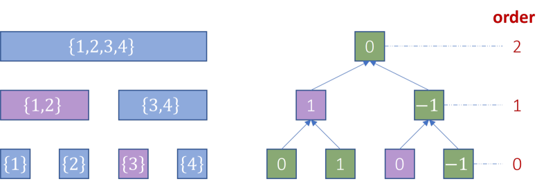
Figure 1. An example with $d=4$ and $k=2$. The left-hand side enumerates all dyadic intervals defined on ${[{d}]}$, with the nodes highlighted in purple representing the dyadic decomposition $\mathcal{C}(3)$ of the interval ${[{3}]}$. The right-hand side enumerates all partial sums for the discrete derivative $X_{u}={({0,1,0,-1})}$, with the nodes highlighted in purple representing the partial sums associated with dyadic intervals in $\mathcal{C}(3)$. ©Olga Ohrimenko, Anthony Wirth, Hao Wu

Example 3.3.

All possible dyadic intervals defined on interval ${[{4}]}$ include $\mathcal{I}_{0,1}=\left\{{1}\right\}$, $\mathcal{I}_{0,2}=\left\{{2}\right\}$, $\mathcal{I}_{0,3}=\left\{{3}\right\}$, $\mathcal{I}_{0,4}=\left\{{4}\right\}$, $\mathcal{I}_{1,1}=\left\{{1,2}\right\}$, $\mathcal{I}_{1,2}=\left\{{3,4}\right\}$, $\mathcal{I}_{2,1}=\left\{{1,2,3,4}\right\}$.

Definition 3.4 (Partial Sum).

For each $h\in[{0}\,.\,.\,{\log d}]$, and each $j\in{[{d/2^{h}}]}$, define for each user the partial sum associated with $\mathcal{I}_{h,j}$ to be

(3) $$S_{u}({\mathcal{I}_{h,j}})\doteq\sum_{\_}{t\in\mathcal{I}_{h,j}}X_{u}{[{t}]},\,\forall u\in[n].$$

and their sum as

(4) $$S({\mathcal{I}_{h,j}})\doteq\sum_{\_}{u\in{[{n}]}}S_{u}({\mathcal{I}_{h,j}})$$

Here, $h$ refers to the order of a partial sum.

Example 3.5.

Suppose that $X_{u}={({0,1,0,-1})}$. The possible partial sums are $S_{u}({\mathcal{I}_{0,1}})=0$, $S_{u}({\mathcal{I}_{0,2}})=1$, $S_{u}({\mathcal{I}_{0,3}})=0$, $S_{u}({\mathcal{I}_{0,4}})=-1$, $S_{u}({\mathcal{I}_{1,1}})=1$, $S_{u}({\mathcal{I}_{1,2}})=-1$, $S_{u}({\mathcal{I}_{2,1}})=0$.

Note that if $S_{u}({\mathcal{I}_{h,j}})\neq 0$, then there is at least one $t\in\mathcal{I}_{h,j}$ for which $X_{u}{[{t}]}\neq 0$. Since dyadic intervals of order $h$ are disjoint, and there are at most $k$ non-zero $X_{u}{[{t}]}$ over all $t\in[d]$, we have this observation:

Observation 3.6.

For each  $h\in[{0}\,.\,.\,{\log d}]$, there can be at most $k$ indices $j\in{[{d/2^{h}}]}$ for which $S_{u}({\mathcal{I}_{h,j}})\neq 0$.

Combining Equation (3) and the fact that $X_{u}{[{t}]}={\text{st}}_{u}{[{t}]}-{\text{st}}_{u}{[{t-1}]}$, and that $\mathcal{I}_{h,j}=\{(j-1)\cdot 2^{h}+1,\ldots,j\cdot 2^{h}\}$, we observe:

Observation 3.7.

For each $u\in[n]$, and $\mathcal{I}_{h,j}\in\textit{ISet}$, we have

(5) $$S_{u}({\mathcal{I}_{h,j}})={\text{st}}_{u}{[{j\cdot 2^{h}}]}-{\text{st}}_{u}{[{(j-1)\cdot 2^{h}}]}\in\left\{{-1,0,1}\right\}\,.$$

Recall that ${\text{st}}_{u}{[{t}]}=\sum_{\_}{t^{\prime}\in{[{t}]}}X_{u}{[{t^{\prime}}]}$. It can be viewed as the cumulative data change from time $1$ to time $t$. If we decompose the interval ${[{t}]}$ into a sequence of disjoint dyadic intervals, then ${\text{st}}_{u}{[{t}]}$ can be expressed as the sum of cumulative changes over these intervals.

Fact 3.8.

(Dyadic Decomposition) For each $t\in{[{d}]}$, the interval ${[{t}]}$ can be decomposed into a minimum collection, $\mathcal{C}(t)$, of at most $\lceil\log t\rceil$ disjoint dyadic intervals with distinct orders.

For example, the dyadic decomposition of the interval ${[{3}]}$ is given by $\left\{{\left\{{1,2}\right\},\left\{{3}\right\}}\right\}$. See Figure 1 for the illustration. In general, for $1\leq\ell\leq r\leq d$, the interval $[{\ell}\,.\,.\,{r}]$ can also be decomposed into a minimum collection of at most $\lceil 2\cdot\log(r-\ell+1)\rceil$ disjoint dyadic intervals. But these intervals might not have distinct orders. For example, the decomposition of the interval $[{2}\,.\,.\,{3}]$ is given by $\left\{{\left\{{2}\right\},\left\{{3}\right\}}\right\}$. Fact 3.8 holds since the interval ${[{t}]}$ starts from $1$.

Via the definition of $\mathcal{C}(t)$, we have ${\text{st}}_{u}{[{t}]}=\sum_{\_}{\mathcal{I}_{h,j}\in\mathcal{C}(t)}S_{u}({\mathcal{I}_{h,j}})$. Summing over $u\in[n]$, and combining this with Equation (1), (3) and (4), we have

Observation 3.9.

For each time $t\in[d]$,

(6) $${a}[t]=\sum_{\_}{u\in{[{n}]}}\sum_{\_}{\mathcal{I}_{h,j}\in\mathcal{C}(t)}S_{u}({\mathcal{I}_{h,j}})=\sum_{\_}{\mathcal{I}_{h,j}\in\mathcal{C}(t)}S({\mathcal{I}_{h,j}}).$$

4. Framework

In this section, we introduce an LDP protocol that achieves our proposed error guarantee. It improves the previously known bound (Úlfar Erlingsson et al., 2020) by a factor of $\sqrt{k}$. The main result of the paper is summarized as follows:

Theorem 4.1.

Assuming that $\varepsilon\leq 1$, and $\varepsilon^{-1}\cdot{({\log d})}\cdot\sqrt{k\cdot\ln{({d/\beta})}}$ $\leq\sqrt{n}$, there is an $\varepsilon$-local differentially private protocol, such that, with probability at least $1-\beta$, its $d$ estimates $\{\hat{{a}}[t]\}$ of $\{{a}[t]\}$ satisfy

$$\max_{\_}{t\in[d]}\left|{\hat{{a}}[t]-{a}[t]}\right|\in O\left(\frac{\log d}{\varepsilon}\cdot\sqrt{k\cdot n\cdot\ln\frac{d}{\beta}}\right)\,.$$

The assumption $\varepsilon^{-1}\cdot{({\log d})}\cdot\sqrt{k\cdot\ln{({d/\beta})}}\leq\sqrt{n}$ ensures that  $\varepsilon^{-1}\cdot{({\log d})}\cdot\sqrt{k\cdot n\cdot\ln{({d/\beta})}}\leq n$, avoiding a trivial bound.

4.1. Overview

Our framework is split between the user (or client) and the server. Each user reports perturbed data to the server, who aggregates the data from all users and computes the required statistics while adjusting for the noise in the reports.

As a warm up consider the following (non-private) naive protocol. Here, each user $u\in{[{n}]}$ computes and reports (to the server) each partial sum $S_{u}({\mathcal{I}_{h,j}})$ immediately after it has all the data needed for the computation. In particular, since the last number in the dyadic interval $\mathcal{I}_{h,j}$ is $j\cdot 2^{h_{\_}u}$, the last data point needed to compute $S_{u}({\mathcal{I}_{h,j}})$ is $X_{u}{[{j\cdot 2^{h_{\_}u}}]}$. Based on the reports of the partial sums, according to Equation (6), the server can obtain for each $t\in[d]$ a precise value of ${a}[t]$.

The naive protocol does not provide LDP guarantees. To this end, our algorithms build on a combination of the following two reporting techniques.

Reporting based on Sampling. Suppose, instead of reporting every partial sum, each user $u\in{[{n}]}$ samples an integer $h_{\_}u\in[{0}\,.\,.\,{\log d}]$ uniformly at random, and reports only the partial sums with order $h_{\_}u$. The server no longer has exact values of the ${a}[t],\forall t\in{[{d}]}$. However, the server can easily construct an unbiased estimate. For each $h\in[{0}\,.\,.\,{\log d}]$, and each $j\in{[{d/2^{h}}]}$, let $z_{\_}u[h,j]$ be the server’s estimate of $S_{u}({\mathcal{I}_{h,j}})$. If it sets $z_{\_}u[h,j]=(1+\log d)\cdot\mathds{1}_{\left[h_{\_}u=h\right]}\cdot S_{u}({\mathcal{I}_{h,j}})$, where $\mathds{1}_{\left[h_{\_}u=h\right]}$ is the indicator for the event $h_{\_}u=h$, then  $z_{\_}u[h,j]$ is an unbiased estimate of $S_{u}({\mathcal{I}_{h,j}})$. Via linearity of expectation, replacing $S_{u}({\mathcal{I}_{h,j}})$ in Equation (6) with $z_{\_}u[h,j]$ gives an unbiased estimator ${a}[t]$.

Reporting with Perturbation. In the previous paragraph, conditioned on $h_{\_}u=h$, user $u\in{[{n}]}$ reports a sequence of $L\doteq d/2^{h}$ partial sums with order $h$ to the server, each taking value in $\left\{{-1,0,1}\right\}$ according to Equation (5). To achieve LDP with this approach, the user $u$ should invoke some randomizer $\mathcal{M}$, to perturb their partial sums before reporting. This also requires a change in computing the estimators $z_{\_}u[h,j]$ with respect to $\mathcal{M}$. Our randomizer, $\mathcal{M}$, exploits sparsity: there are at most $k$ non-zero partial sums with order $h$ (Observation 3.6).

4.2. Client Side

Randomizer. Let $\mathcal{M}$ be a client-side randomizer. Our protocol relies on a randomizer $\mathcal{M}$ that provides the following functionalities and has three properties described below.

$\mathcal{M}$ has an (optional) initialization phase $\mathcal{M}.\textit{init}(L,k,\varepsilon)$, with parameters the length of the input $L$, the maximum number of non-zero elements in the input $k$, and the privacy budget $\varepsilon$. In this phase, $\mathcal{M}$ can perform some pre-computation whose result is kept for reference later.

During the protocol, $\mathcal{M}$ takes as input a sequence $v_{\_}1,\ldots,v_{\_}L$ where each value is in $\{-1,0,1\}$, corresponding to user’s data, and outputs a sequence $\mathcal{M}^{(1)}(v_{\_}1),\ldots,\mathcal{M}^{(L)}(v_{\_}L)\in\{-1,1\}$. The output of $\mathcal{M}^{(j)}(v_{\_}j)$ may depend not only on the input $v_{\_}j$ and the randomness of $\mathcal{M}^{(j)}$, but also on the pre-computation result, the past inputs $v_{\_}1,\dots,v_{\_}{j-1}$ and outputs $\mathcal{M}^{(1)}(v_{\_}1),\ldots,\mathcal{M}^{(j-1)}(v_{\_}{j-1})$.

Finally, $\mathcal{M}$ should satisfy the following three properties.

Property I.: Given $L$, $k$ and $\varepsilon\leq 1$, there exists $p_{\text{min}},p_{\text{max}}\in{({0,1})}$, such that $p_{\text{max}}/p_{\text{min}}\leq e^{\varepsilon}$, and that for each $k$-sparse input sequence $v_{\_}1,\ldots,v_{\_}L\in\left\{{-1,0,1}\right\}$, and each sequence $w_{\_}1,\ldots,$ $w_{\_}L\in\left\{{-1,1}\right\}$, (7) $$\Pr[M^{(1)}(v_{\_}1)=w_{\_}1,\ldots,M^{(L)}(v_{\_}L)=w_{\_}L]\in{[{p_{\text{min}},p_{\text{max}}}]}\,.$$ Property II. : There exits $c_{\text{gap}}\in{({0,1})}$, such that for all $j\in{[{L}]}$, if $v_{\_}j\neq 0$, (8) $$\Pr[\mathcal{M}^{(j)}(v_{\_}j)=v_{\_}j]-\Pr[\mathcal{M}^{(j)}(v_{\_}j)=-v_{\_}j]=c_{\text{gap}}\,.$$ Property III.: For all $j\in{[{L}]}$, if $v_{\_}j=0$, (9) $$\Pr[\mathcal{M}^{(j)}(v_{\_}j)=1]=\Pr[\mathcal{M}^{(j)}(v_{\_}j)=-1]=\frac{1}{2}\,.$$

Example 4.2.

The following randomizer (Warner, 1965) satisfies these three properties. Suppose that $\mathcal{M}$ perturbs each coordinate independently such that: if $v_{\_}j\neq 0$, then $\Pr[\mathcal{M}^{(j)}(v_{\_}j)=v_{\_}j]=e^{\varepsilon/k}/{({e^{\varepsilon/k}+1})}$ and $\Pr[\mathcal{M}^{(j)}(v_{\_}j)=-v_{\_}j]=1/{({e^{\varepsilon/k}+1})}$; if $v_{\_}j=0$, then $\mathcal{M}^{(j)}(v_{\_}j)$ outputs $-1$ or $1$, uniformly at random. Now, Property II and Property III are clearly satisfied with $c_{\text{gap}}={({e^{\varepsilon/k}-1})}/{({e^{\varepsilon/k}+1})}$. Finally, it can be verified that Property I is satisfied, with $p_{\text{min}}=2^{-(L-k)}\cdot{({e^{\varepsilon/k}+1})}^{-k}$ and $p_{\text{max}}=e^{\varepsilon}\cdot 2^{-(L-k)}\cdot{({e^{\varepsilon/k}+1})}^{-k}$.

This simple randomizer does not perform pre-computation in the initialization phase, and for each $j\in{[{L}]}$, the result of $\mathcal{M}^{(j)}(v_{\_}j)$ does not depend on historical inputs or outputs.

Intuitively, Property I states that, regardless of the input sequence, each sequence in $\left\{{-1,1}\right\}^{L}$ is output by $\mathcal{M}$ with similar probability (up to a factor of $e^{\varepsilon}$), by which the client-side algorithm is differentially private. Property II ensures that $\mathcal{M}$ preserves each non-zero coordinate of the input sequences with a common probability; indeed, $c_{\text{gap}}$ is the common difference between the coordinate preservation and reversal probabilities. Property III requires that $\mathcal{M}$ outputs $1$ and $-1$ with equal probability for each zero coordinate. Based on Property II and Property III:

Observation 4.3.

For $v_{\_}j\in\left\{{-1,0,1}\right\}$, it always holds that

(10) $$\operatorname*{\mathbb{E}}\left[{({c_{\text{gap}}})}^{-1}\cdot\mathcal{M}^{(j)}(v_{\_}j)\right]=v_{\_}j.$$

Since $\mathcal{M}^{(j)}(v_{\_}j)$ is in $[-1,1]$; multiplying it by ${({c_{\text{gap}}})}^{-1}$ amplifies the range to ${[{-{({c_{\text{gap}}})}^{-1},{({c_{\text{gap}}})}^{-1}}]}$. As will be explained in Section 4.3, this range plays a vital role in utility analysis. The smaller this range, the better utility we can obtain. Since $\varepsilon\leq 1$, the randomizer in Example 4.2 guarantees ${({c_{\text{gap}}})}^{-1}={({e^{\varepsilon/k}+1})}/{({e^{\varepsilon/k}-1})}\in O{({k/\varepsilon})}$, or equivalently, $c_{\text{gap}}\in\Omega{({\varepsilon/k})}$. Our protocol relies on a randomizer, FutureRand, with a $\sqrt{k}$-better guarantee than this naive one.

Theorem 4.4 (FutureRand).

There is a randomizer $\mathcal{M}$, called FutureRand, that satisfies the above conditions with

(11) $$c_{\text{gap}}\in\Omega{({\varepsilon/\sqrt{k}})}.$$

The design of FutureRand is non-trivial, and we defer it to Section 5. For now, we apply it to complete the design of our longitudinal data tracking protocol.

Client-Side Algorithm. The client-side algorithm is described in Algorithm 1. Each user $u$ first samples an integer $h_{\_}u\in[{0}\,.\,.\,{\log d}]$ uniformly at random and reports it to the server. Then $u$ initializes a zero vector $\boldsymbol{\omega}_{\_}u$, of size $L\doteq d/2^{h_{\_}u}=\left|{\textit{ISet}[{h_{\_}u}]}\right|$ for the dyadic intervals with order $h_{\_}u$. They also initialize a randomizer $\mathcal{M}$, with parameters $L$, $k$ and $\varepsilon$.

The user reports to the server at time $t\in[d]$ if and only if $2^{h_{\_}u}$ divides $t$. In particular, the user $u$ computes partial sum $S_{u}({\mathcal{I}_{h,j}})$ associated with the $j\doteq t/2^{h_{\_}u}$-th dyadic interval $\mathcal{I}_{h_{\_}u,j}$, with order $h_{\_}u$. Note that each multiple of $2^{h_{\_}u}$ is the first time that $u$ has all data $X_{u}{[{t^{\prime}}]}$ needed to compute $S_{u}({\mathcal{I}_{h_{\_}u,j}})$, since by definition:

$$\mathcal{I}_{h_{\_}u,j}=\left\{{{({j-1})}\cdot 2^{h_{\_}u}+1,\ldots,j\cdot 2^{h_{\_}u}}\right\}=\left\{{t-2^{h_{\_}u}+1,\ldots,t}\right\}\,,$$

and $S_{u}({\mathcal{I}_{h_{\_}u,j}})=\sum_{\_}{t^{\prime}\in\mathcal{I}_{h_{\_}u,j}}X_{u}{[{t^{\prime}}]}$. This partial sum is then perturbed by the randomizer $\mathcal{M}^{(j)}$. The perturbed value is stored in $\boldsymbol{\omega}_{\_}u[j]$ and reported to the server.

Algorithm 1 Client $\mathcal{A}_{\text{clt}}{}$

1:User Data $X_{u}$; Privacy parameter $\varepsilon$.

2:report $h_{\_}u\overset{r}{\leftarrow}[{0}\,.\,.\,{\log d}]$. $\triangleright$ Send $h_{\_}u$ to the server

3:Set $L\leftarrow d/2^{h_{\_}u}$ and $\boldsymbol{\omega}_{\_}u\leftarrow\left\{{0}\right\}^{L}$.

4:$\mathcal{M}.\textit{init}(L,k,\varepsilon)$

5:for each time $t\in[d]$ do$\triangleright$ User data $X_{u}[t]$ arrives

6:     if $2^{h_{\_}u}$ divides $t$ then

7:         $j\leftarrow t/2^{h_{\_}u}$

8:         Compute the $j^{(th)}$ partial sum $S_{u}({\mathcal{I}_{h,j}})$.

9:          report $\boldsymbol{\omega}_{\_}u[j]\leftarrow\mathcal{M}^{(j)}{({S_{u}({\mathcal{I}_{h,j}})})}$      

Privacy Guarantee. The privacy guarantee of Algorithm 1 is an immediate consequence of Property I.

Theorem 4.5.

$\mathcal{A}_{\text{clt}}$ is $\varepsilon$-differentially private.

Proof of Theorem 4.5.

Consider a user $u\in{[{n}]}$ with data $X_{u}$. For each $h\in[{0}\,.\,.\,{\log d}]$, we have $\Pr[h_{\_}u=h]$ $=1/{({1+\log d})}$, and, conditioned on $h_{\_}u=h$, we have $L=d/2^{h}$. Via Inequality (7), there exist $p_{\text{min}},p_{\text{max}}\in{({0,1})}$, s.t., $p_{\text{max}}\leq e^{\varepsilon}\cdot p_{\text{min}}$ and that for each $w\in\{-1,1\}^{L}$, it holds that

$$\Pr[\boldsymbol{\omega}_{\_}u[1]=w_{\_}1,\ldots,\boldsymbol{\omega}_{\_}u[L]=w_{\_}L\mid h_{\_}u=h]\in{[{p_{\text{min}},p_{\text{max}}}]}.$$

Suppose that data $X_{u}$ of user $u$ is instead $X_{u}^{\prime}$, with other inputs unchanged. Running $\mathcal{A}_{\text{clt}}$ based on $X_{u}^{\prime}$, we have $h_{\_}u^{\prime}$ and $\boldsymbol{\omega}_{\_}u^{\prime}$ and thus $\Pr[h_{\_}u^{\prime}=h]$ $=1/(1+\log d)$ and that

$$\Pr[\boldsymbol{\omega}_{\_}u^{\prime}[1]=w_{\_}1,\ldots,\boldsymbol{\omega}_{\_}u^{\prime}[L]=w_{\_}L\mid h_{\_}u^{\prime}=h]\in{[{p_{\text{min}},p_{\text{max}}}]}.$$

Since $p_{\text{max}}\leq e^{\varepsilon}\cdot p_{\text{min}}$, the ratio of outcome probabilities is

$$e^{-\varepsilon}\leq\frac{\Pr[h_{\_}u=h,\boldsymbol{\omega}_{\_}u[1]=w_{\_}1,\ldots,\boldsymbol{\omega}_{\_}u[L]=w_{\_}L]missing}{\Pr[h_{\_}u^{\prime}=h,\boldsymbol{\omega}_{\_}u^{\prime}[1]=w_{\_}1,\ldots,\boldsymbol{\omega}_{\_}u^{\prime}[L]=w_{\_}L]missing}\leq e^{\varepsilon}\,.$$

Since the output space of $\mathcal{A}_{\text{clt}}$ is discrete, it satisfies Inequality (2), and therefore is differentially private (Definition 2.2). ∎

4.3. Server Side

Server-Side Algorithm. The server-side algorithm is described in Algorithm 2. At the beginning of the algorithm, according to $\mathcal{A}_{\text{clt}}$ (Algorithm 1, line 2), we assume that the server has received the $n$ sampled orders $h_{\_}1,\ldots,h_{\_}n$, one from each user. The server partitions the users into $1+\log d$ subsets $\mathcal{U}_{\_}0,\ldots,\mathcal{U}_{\_}{\log d}$, such that $\mathcal{U}_{\_}h\doteq\{u\in{[{n}]}:h_{\_}u=h\}$ consists of the subset of users whose sampled orders equal $h$. Observe that each user $u\in\mathcal{U}_{\_}h$ reports their perturbed partial sums $\boldsymbol{\omega}_{\_}u[1],\boldsymbol{\omega}_{\_}u[2]$, $\ldots,\boldsymbol{\omega}_{\_}u[d/2^{h}]$, at times $2^{h},2\cdot 2^{h},\ldots,d$, respectively.

Algorithm 2 Server $\mathcal{A}_{\text{svr}}$

1:Reports $(h_{\_}u,\boldsymbol{\omega}_{\_}u)$ from the users.

2:$\mathcal{U}_{\_}h\leftarrow\{u\in{[{n}]}:h_{\_}u=h\},\forall h\in[{0}\,.\,.\,{\log d}]$.

3:for each time $t\in[d]$ do

4:     for $h\in[{0}\,.\,.\,{\log d}]$ s.t. $2^{h}$ divides $t$ do

5:         $j\leftarrow t/2^{h}$

6:          $\hat{S}({\mathcal{I}_{h,j}})\leftarrow\sum_{\_}{u\in\mathcal{U}_{\_}h}(1+\log d)\cdot{({c_{\text{gap}}})}^{-1}\cdot\boldsymbol{\omega}_{\_}u[j]$      

7:      output $\hat{{a}}[t]\leftarrow\sum_{\_}{\mathcal{I}_{h,j}\in\mathcal{C}(t)}\hat{S}({\mathcal{I}_{h,j}})$

Based on user reports, for each $u\in{[{n}]},h\in[{0}\,.\,.\,{\log d}],j\in{[{d/2^{h}}]}$, consider this estimator $z_{\_}u[h,j]$ of $S_{u}({\mathcal{I}_{h,j}})$. If $h_{\_}u=h$, then $z_{\_}u[h,j]=(1+\log d)\cdot{({c_{\text{gap}}})}^{-1}\cdot\boldsymbol{\omega}_{\_}u[j]$; otherwise, $z_{\_}u[h,j]=0$. Since $\boldsymbol{\omega}_{\_}u[j]\in\left\{{-1,1}\right\}$, it holds that $z_{\_}u[h,j]\in(1+\log d)\cdot{({c_{\text{gap}}})}^{-1}\cdot{[{-1,1}]}$. Further, the expectation of $z_{\_}u[h,j]$ is given by

$$\operatorname*{\mathbb{E}}\left[z_{\_}u[h,j]\right]=\Pr[h_{\_}u=h]\cdot(1+\log d)\cdot\operatorname*{\mathbb{E}}\left[{({c_{\text{gap}}})}^{-1}\cdot\boldsymbol{\omega}_{\_}u[j]\right]\,.$$

Noting that $\boldsymbol{\omega}_{\_}u[j]=\mathcal{M}^{(j)}{({S_{u}({\mathcal{I}_{h,j}})})}$, and via Equation (10), we see

(12) $$\operatorname*{\mathbb{E}}\left[z_{\_}u[h,j]\right]=S_{u}({\mathcal{I}_{h,j}})\,.$$

Via linearity of expectation, $\hat{S}({\mathcal{I}_{h,j}})=\sum_{\_}{u\in{[{n}]}}z_{\_}u[h,j]$ is an unbiased estimator of $S({\mathcal{I}_{h,j}})$. Keeping only the non-zero terms, and replacing $z_{\_}u[h,j]$ with its definition, we have

$$\hat{S}({\mathcal{I}_{h,j}})=\sum_{\_}{u\in\mathcal{U}_{\_}h}(1+\log d)\cdot{({c_{\text{gap}}})}^{-1}\cdot\boldsymbol{\omega}_{\_}u[j]\,,$$

which justifies the update rule of $\hat{S}({\mathcal{I}_{h,j}})$ (Algorithm 2, line 6). Finally, replacing $S({\mathcal{I}_{h,j}})$ with $\hat{S}({\mathcal{I}_{h,j}})$ in Equation (6) gives an unbiased estimator, $\hat{{a}}[t]=\sum_{\_}{\mathcal{I}_{h,j}\in\mathcal{C}(t)}\hat{S}({\mathcal{I}_{h,j}})$, of ${a}[t]$ (Algorithm 2, line 7).

Utility Guarantee. We conclude that $\hat{{a}}[t]$ is an unbiased estimator of ${a}[t]$; how often is it accurate?

Lemma 4.6.

For each $t\in[d]$, assuming that $\varepsilon\leq 1$ and that $\sqrt{n}\geq{({c_{\text{gap}}})}^{-1}\cdot\log d\cdot\sqrt{\ln{({1/\beta^{\prime}})}}$, with probability at least $1-\beta^{\prime}$, the estimates $\hat{{a}}[t]$ computed as in Algorithm 2 satisfy

$$|\hat{{a}}[t]-{a}[t]|\in O\left({({c_{\text{gap}}})}^{-1}\cdot\log d\cdot\sqrt{n\cdot\ln\frac{1}{\beta^{\prime}}}\right)$$

We first prove our main Theorem 4.1 based on Theorems 4.4 and Lemma 4.6, then justify Lemma 4.6.

Proof of Theorem 4.1.

Via Theorem 4.4, we know that $c_{\text{gap}}\in\Omega{({\varepsilon/\sqrt{k}})}$. Therefore, ${({c_{\text{gap}}})}^{-1}\in O{({\sqrt{k}/\varepsilon})}$. Applying Lemma 4.6 with $\beta^{\prime}=\beta/d$, and via union bound, we conclude that, with probability at least $1-\beta$,

$$\max_{\_}{t\in{[{d}]}}|\hat{{a}}[t]-{a}[t]|\in O\left(\frac{\log d}{\varepsilon}\cdot\sqrt{k\cdot n\cdot\ln\frac{d}{\beta}}\right).$$

∎

Proof of Lemma 4.6.

First, rewrite

$$\hat{{a}}[t] =\sum_{\_}{\mathcal{I}_{h,j}\in\mathcal{C}(t)}\hat{S}({\mathcal{I}_{h,j}})=\sum_{\_}{\mathcal{I}_{h,j}\in\mathcal{C}(t)}\sum_{\_}{u\in{[{n}]}}z_{\_}u[h,j]\,.$$

For each $u\in{[{n}]}$, define $Y_{\_}u=\sum_{\_}{\mathcal{I}_{h,j}\in\mathcal{C}(t)}z_{\_}u[h,j]$. Exchanging the order of summation gives $\hat{{a}}[t]=\sum_{\_}{u\in{[{n}]}}Y_{\_}u$. Clearly the $Y_{\_}u$ are independent. We claim (proven below): $Y_{\_}u\in(1+\log d)\cdot{({c_{\text{gap}}})}^{\cdot}[-1,1]$. Then applying Hoeffding’s Inequality (Corollary A.2), and the fact that $\operatorname*{\mathbb{E}}\left[\hat{{a}}[t]\right]={a}[t]$, we see that with probability at most $\beta^{\prime}$,

(13) $$\left|{\hat{{a}}[t]-{a}[t]}\right|\geq(1+\log d)\cdot{({c_{\text{gap}}})}^{-1}\cdot\sqrt{2n\cdot\ln\frac{2}{\beta^{\prime}}}\,.$$

We prove the claim, that $Y_{\_}u\in(1+\log d)\cdot{({c_{\text{gap}}})}^{-1}\cdot[-1,1]$. By Fact 3.8, dyadic intervals in $\mathcal{C}(t)$ have distinct orders. By definition, $z_{\_}u[h,j]$ is non-zero exactly when $h_{\_}u=h$, so among all $\mathcal{I}_{h,j}\in\mathcal{C}(t)$, there is at most one non-zero $z_{\_}u[h,j]$. Its value either $-(1+\log d)\cdot{({c_{\text{gap}}})}^{-1}$ or $(1+\log d)\cdot{({c_{\text{gap}}})}^{-1}$. ∎

5. Randomizer

In this section, we present a randomizer, the FutureRand, denoted briefly by $\mathcal{M}$, that satisfies Theorem 4.4. The FutureRand is based on two techniques, composition for randomized responses (for non-zero coordinates) and pre-computation for the composition.

5.1. Overview

The input to $\mathcal{M}$ is a $k$-sparse sequence $v={({v_{\_}1,\ldots,v_{\_}L})}\in\{-1,0,1\}^{L}$, and the output is sequence $\mathcal{M}^{(1)}(v_{\_}1),\ldots,\mathcal{M}^{(L)}(v_{\_}L)\in\{-1,1\}^{L}$. Denote the support of $v$ as $\text{supp}(v)\doteq\left\{{j\in[L]:v_{\_}j\neq 0}\right\}$.

Zero Coordinates. For each $j\notin\text{supp}(v)$, $\mathcal{M}^{(j)}(v_{\_}j)$ outputs $-1$ and $1$ uniformly at random. Hence Property III is trivially satisfied.

Non-Zero Coordinates. The presentation of FutureRand to handle non-zero coordinates follows three steps.

• Offline Input with Fixed Support Size. First we assume that all coordinates of $v$ are inputted to $\mathcal{M}$ simultaneously, and that the $v$ contains exactly $k$ non-zero coordinates.

• Online Input with Fixed Support Size. We convert the protocol to online, where each coordinate $v_{\_}j$ arrives one by one, and $\mathcal{M}$ outputs the perturbed value of $v_{\_}j$ immediately.

• Online Input with Bounded Support Size. We show that Online Input with Fixed Support Size protocol provides the same guarantees even when $v$ has support less than $k$.

For each step, we need to show that the $\mathcal{M}$ constructed satisfies Property I, Property II with $c_{\text{gap}}\in\Omega{({\varepsilon/\sqrt{k}})}$.

5.2. Offline Input with Fixed Support Size

By assumption, $v$ contains $k$ non-zero coordinates. $\mathcal{M}$ invokes a subroutine, $\tilde{\mathcal{R}}:\left\{{-1,1}\right\}^{k}\rightarrow\left\{{-1,1}\right\}^{k}$ to perturb these coordinates. $\tilde{\mathcal{R}}$ is a composed randomizer: instead of perturbing each coordinate independently, it adds correlated noise to the coordinates. The building block of $\tilde{\mathcal{R}}$ is a basic randomizer $\mathcal{R}$. The pseudo-codes of both $\mathcal{R}$ and $\tilde{\mathcal{R}}$ are described in Algorithm 3.

Basic Randomizer $\mathcal{R}$ (Warner, 1965). For each $\zeta\in\left\{{-1,1}\right\}$.

(14) $$\mathcal{R}(\zeta)=\begin{cases}\zeta,&\text{w.p.}\,e^{\tilde{\varepsilon}}/{({e^{\tilde{\varepsilon}}+1})}\\ -\zeta,&\text{w.p.}\,1/{({e^{\tilde{\varepsilon}}+1})}\end{cases},$$

where $\tilde{\varepsilon}$ depends on $\varepsilon$, defined later.

Composed Randomizer $\tilde{\mathcal{R}}$. For an input $b\in\left\{{-1,1}\right\}^{k}$, it first applies $\mathcal{R}$ independently to each coordinate of $b$. Denote the result by $b^{\prime}=\mathcal{R}(b)\doteq{({\mathcal{R}(b_{\_}1),\ldots,\mathcal{R}(b_{\_}k)})}$. Denote $p\doteq 1/(e^{\tilde{\varepsilon}}+1)$. In expectation, $\left\|{b^{\prime}-b}\right\|_{\_}0=kp$. Let

(15) $$\text{LB}\doteq kp-2\sqrt{k},\,\quad\text{UB}\doteq\frac{k}{\tilde{\varepsilon}}\cdot\ln\frac{2e^{\tilde{\varepsilon}}}{e^{\tilde{\varepsilon}}+1}\,.$$

Next, define the set of sequences whose $\ell_{\_}0$-distance (Hamming distance) to $b$ is within $[{\text{LB}}\,.\,.\,{\text{UB}}]$.

Definition 5.1 (Annulus).

Given $b\in\left\{{-1,1}\right\}^{k}$, denote

$$\textbf{Ann}(b)\doteq\left\{{s\in\left\{{-1,1}\right\}^{k}:\left\|{b-s}\right\|_{\_}0\in[{\text{LB}}\,.\,.\,{\text{UB}}]}\right\}.$$

If $b^{\prime}\notin\textbf{Ann}(b)$, $\tilde{\mathcal{R}}$ replaces it with a uniform sample from $\left\{{-1,1}\right\}^{k}\setminus\textbf{Ann}(b)$. Finally, $\tilde{\mathcal{R}}$ outputs $b^{\prime}$.

Randomizer $\tilde{\mathcal{R}}$ has the following privacy and utility guarantees, the analysis of which is deferred to Section 5.5.

Lemma 5.2.

Suppose that $\varepsilon\leq 1$ and let $\tilde{\varepsilon}=\varepsilon/{({5\sqrt{k}})}$. There exist $p_{\text{min}}^{\prime},p_{\text{max}}^{\prime}\in{({0,1})}$ with $p_{\text{max}}^{\prime}\leq e^{\varepsilon}\cdot p_{\text{min}}^{\prime}$, such that for each input sequence $b\in\left\{{-1,1}\right\}^{k}$, and each sequence $s\in\left\{{-1,1}\right\}^{k}$,

(16) $$\Pr[\tilde{\mathcal{R}}(b)=s]\in{[{p_{\text{min}}^{\prime},p_{\text{max}}^{\prime}}]}\,.$$

for $\tilde{\mathcal{R}}(b)$ as defined in Algorithm 3.

Lemma 5.3.

For a given input $b$, denote $\tilde{b}\doteq\tilde{\mathcal{R}}(b)$ the output of $\tilde{\mathcal{R}}$. There exits some $c_{\text{gap}}\in\Omega{({\tilde{\varepsilon}})}=\Omega{({\varepsilon/\sqrt{k}})}$, such that for each input $b\in\left\{{-1,1}\right\}^{k}$, and for each $i\in{[{k}]}$,

(17) $$\Pr[\tilde{b}_{\_}i=b_{\_}i]-\Pr[\tilde{b}_{\_}i=-b_{\_}i]=c_{\text{gap}}\in\Omega{({\varepsilon/\sqrt{k}})}\,.$$

Algorithm 3 FutureRand  $\mathcal{M}$, describing $\tilde{\mathcal{R}}$

1:Procedure Basic Randomizer $\mathcal{R}$($\zeta$)

2:Value $\zeta\in\left\{{-1,1}\right\}$.

3:     return $-\zeta$ w.p. $1/{({e^{\tilde{\varepsilon}}+1})}$ and $\zeta$ w.p. $e^{\tilde{\varepsilon}}/{({e^{\tilde{\varepsilon}}+1})}$.

4:

5:Procedure Composed Randomizer $\tilde{\mathcal{R}}$($b$)

6:Vector $b\in\left\{{-1,1}\right\}^{k}$.

7:     Sample $b^{\prime}\leftarrow{({\mathcal{R}(b_{\_}1),\ldots,\mathcal{R}(b_{\_}k)})}$.

8:     if  $b^{\prime}\notin\textbf{Ann}(b)$  then

9:         $b^{\prime}\overset{r}{\leftarrow}\left\{{-1,1}\right\}^{k}\setminus\textbf{Ann}(b)$      

10:     return $b^{\prime}$

11:

12:Procedure $\mathcal{M}.\textit{init}$($L,k,\varepsilon$)

13:Input length $L$; Support size $k$; Privacy parameter $\varepsilon$

14:     Set $\tilde{\varepsilon}\leftarrow\varepsilon/{({5\sqrt{k}})}$.

15:     Set $\tilde{b}\leftarrow\tilde{\mathcal{R}}(1^{k})$.

16:     Set $\mathsf{nnz}\leftarrow 0$.

17:

18:Procedure $\mathcal{M}^{(j)}$($v_{\_}j$)$\triangleright$ $j=1,2,\ldots,L$

19:Value $v_{\_}j\in\left\{{-1,0,1}\right\}$.

20:     if $v_{\_}j\neq 0$ then

21:         $\mathsf{nnz}\leftarrow\mathsf{nnz}+1$.

22:         return $v_{\_}j\cdot\tilde{b}_{\_}{\mathsf{nnz}}$.

23:     else

24:         return $-1$ or $+1$ uniformly at random.      

Analysis. Since $\mathcal{M}$ perturbs the non-zero coordinates of input $v$ with $\tilde{\mathcal{R}}$, Property II is satisfied based on the Lemma 5.3. Hence, it is left to verify Property I. Consider an arbitrary sequence $w_{\_}1,\ldots,w_{\_}L\in\left\{{-1,1}\right\}$. The event

$$E:M^{(1)}(v_{\_}1)=w_{\_}1,\ldots,M^{(L)}(v_{\_}L)=w_{\_}L$$

can be decomposed into two events:

1. $E_{\_}1:$ $\forall j\notin\text{supp}(v)$, $\mathcal{M}^{(j)}(v_{\_}{j})=w_{\_}{j}$.

2. $E_{\_}2:$ $\forall j\in\text{supp}(v)$, $\mathcal{M}^{(j)}(v_{\_}{j})=w_{\_}{j}$.

We have $\Pr[E_{\_}1]=2^{-{({L-k})}}$ as the $\mathcal{M}^{(j)}(v_{\_}{j})$ values are independent in $\{-1,+1\}$ for $j\notin\text{supp}(v)$. To bound $\Pr[E_{\_}2]$, denote the indices in $\text{supp}(v)$ as $j_{\_}1<\cdots<j_{\_}k$. Since $\mathcal{M}$ perturbs the non-zero coordinates with $\tilde{\mathcal{R}}$, applying Lemma 5.2 with input $b={({v_{\_}{j_{\_}1},\ldots,v_{\_}{j_{\_}k}})}$ and output $s={({w_{\_}{j_{\_}1},\ldots,w_{\_}{j_{\_}k}})}$, it holds that $\Pr[E_{\_}2]=\Pr[\tilde{\mathcal{R}}(b)=s]\in{[{p_{\text{min}}^{\prime},p_{\text{max}}^{\prime}}]}$. Since $E_{\_}1$ and $E_{\_}2$ are independent, we have

(18) $$\Pr[E]=\Pr[E_{\_}1]\cdot\Pr[E_{\_}2]\in 2^{-{({L-k})}}\cdot{[{p_{\text{min}}^{\prime},p_{\text{max}}^{\prime}}]}\,,$$

which proves Property I.

5.3. Online Input with Fixed Support Size

In this step, we modify $\mathcal{M}$ into an online algorithm, where each coordinate $v_{\_}j$ arrives one by one, and $\mathcal{M}$ is required to perturb and output each coordinate immediately after its arrival. Since $\mathcal{M}$ perturbs the zero coordinates independently, we only need to take care of the non-zero coordinates. We develop a new pre-computation technique to generate the correlated noises for the non-zero elements in the initialization phase. With these noises, we perturb the non-zero coordinates as they arrive. This motivates the design of $\mathcal{M}.\textit{init}{({L,k,\varepsilon})}$ and $\mathcal{M}^{(j)}{({v_{\_}j})}$, $j\in{[{L}]}$, whose pseudo-codes are in Algorithm 3.

$\mathcal{M}.\textit{init}{({L,k,\varepsilon})}$. The procedure takes as parameters $L$, the size of the input sequence; $k$, the maximum number of non-zero elements in the input sequence; and $\varepsilon$, the privacy parameter. It sets $\tilde{\varepsilon}$ as $\varepsilon/{({5\ \sqrt{k}})}$, and invokes the composed randomizer $\tilde{\mathcal{R}}$ with the vector $1^{k}$ consisting of all ones. The returned sequence is kept as a vector $\tilde{b}$. Finally, the procedure creates a variable $\mathsf{nnz}$ with value $0$; the variable $\mathsf{nnz}$ is shared by other procedures, to keep track of the support of the input sequence received so far.

$\mathcal{M}^{(j)}{({v_{\_}j})}$. For all $j\in{[{L}]}$, $\mathcal{M}^{(j)}{({v_{\_}j})}$ shares the same pseudo-codes. If $v_{\_}j=0$, the procedure outputs $-1$ or $+1$, uniformly at random. Otherwise, it increases $\mathsf{nnz}$ by $1$, indicating that $v_{\_}j$ is the ${({\mathsf{nnz}})}^{(th)}$ non-zero entry processed by the procedure. Then it outputs the value of $v_{\_}j$ multiplied by $\tilde{b}_{\_}{\mathsf{nnz}}$.

Analysis. We need to prove that Property I and Property II hold. Consider the events $E_{\_}1$ and $E_{\_}2$ defined as before. We see that $\Pr[E_{\_}1]$ remains the same. Denote the indices in $\text{supp}(v)$ as $j_{\_}1<\cdots<j_{\_}k$. Based on our modification, for each $i\in{[{k}]}$, we have $\mathcal{M}^{(j_{\_}i)}(v_{\_}{j_{\_}i})=\tilde{b}_{\_}i\cdot v_{\_}{j_{\_}i}$. Hence, event $E_{\_}2$ holds only if for each $i\in{[{k}]}$, $\tilde{b}_{\_}i\cdot v_{\_}{j_{\_}i}=w_{\_}{j_{\_}i}$, equivalently, $\tilde{b}_{\_}i=w_{\_}{j_{\_}i}/v_{\_}{j_{\_}i}$. Since $\tilde{b}=\tilde{\mathcal{R}}(1^{k})$, applying Lemma 5.2 with $s={({w_{\_}{j_{\_}1}/v_{\_}{j_{\_}1},\ldots,w_{\_}{j_{\_}k}/v_{\_}{j_{\_}k}})}$, it holds that

$$\Pr[E_{\_}2]=\Pr[\tilde{b}=s]=\Pr[\tilde{\mathcal{R}}(1^{k})=s]\in{[{p_{\text{min}}^{\prime},p_{\text{max}}^{\prime}}]}\,.$$

It follows that Inequality (18) still holds, and therefore Property I.

Finally, observe that $\mathcal{M}^{(j_{\_}i)}(v_{\_}{j_{\_}i})=v_{\_}{j_{\_}i}$ if $\tilde{b}_{\_}i=1$; and $\mathcal{M}^{(j_{\_}i)}(v_{\_}{j_{\_}i})=-v_{\_}{j_{\_}i}$ if $\tilde{b}_{\_}i=-1$. Since $\tilde{b}=\tilde{\mathcal{R}}{({1^{k}})}$, we have $\Pr[\tilde{b}_{\_}i=1]-\Pr[\tilde{b}_{\_}i=-1]=c_{\text{gap}}$. Therefore, Property II holds with $c_{\text{gap}}\in\Omega{({\varepsilon/\sqrt{k}})}$.

5.4. Online Input with Bounded Support Size

In this step, we relax the constraint that vector $v$ contains exactly $k$ non-zero coordinates. In particular, we show that Property I and Property II still hold, if the same protocol discussed in Section 5.3 acts on input with support less than $k$. In the case $\left|{\text{supp}(v)}\right|=k$, each bit of the pre-generated vector $\tilde{b}=\tilde{\mathcal{R}}(1^{k})$ is used to multiply some non-zero coordinate of $v$. In the case $\left|{\text{supp}(v)}\right|<k$, however, only the first $\left|{\text{supp}(v)}\right|$ bits of $\tilde{b}$ are used.

Analysis. With a similar argument as previous section, Property II holds with $c_{\text{gap}}\in\Omega{({\varepsilon/\sqrt{k}})}$. To verify Property I, we prove that Inequality (18) still holds. Consider the events $E_{\_}1$ and $E_{\_}2$ defined as before. We have $\Pr[E_{\_}1]=2^{-(L-\left|{\text{supp}(v)}\right|)}$ as the $\mathcal{M}^{(j)}(v_{\_}{j})$ variables are independent in $\{-1,1\}$ random variables for $j\notin\text{supp}(v)$. The event $E_{\_}2$ happens if only for each $i\in{[{\left|{\text{supp}(v)}\right|}]}$, it holds that $\tilde{b}_{\_}i={w_{\_}{j_{\_}i}}/{v_{\_}{j_{\_}i}}$. Let $\mathcal{G}$ be the subset of sequence $s\in\left\{{-1,1}\right\}^{k}$ which satisfies $s_{\_}i={w_{\_}{j_{\_}i}}/{v_{\_}{j_{\_}i}}$, for each $i\in{[{\left|{\text{supp}(v)}\right|}]}$. There are $2^{k-\left|{\text{supp}(v)}\right|}$ such possible sequences, each being outputted by $\tilde{\mathcal{R}}{({1^{k}})}$ with probability between ${[{p_{\text{min}}^{\prime},p_{\text{max}}^{\prime}}]}$ (by Lemma 5.2). Therefore,

$$\Pr[E_{\_}2]=\Pr[\tilde{b}\in\mathcal{G}]\in 2^{k-\left|{\text{supp}(v)}\right|}\cdot{[{p_{\text{min}}^{\prime},p_{\text{max}}^{\prime}}]}.$$

Multiplying it by $\Pr[E_{\_}1]=2^{-(L-\left|{\text{supp}(v)}\right|)}$ proves Inequality (18).

5.5. Sketch Proofs

We conclude the technical presentation with outlines of our proofs for Lemma 5.2 and 5.3. The complete proofs for Lemma 5.2 and 5.3 are included in Appendix A.1.1 and A.1.2, respectively.

We use the following notation. As before, denote $p=1/(e^{\tilde{\varepsilon}}+1)$. Note that $1-p=e^{\tilde{\varepsilon}}p$. For each $i\in[{0}\,.\,.\,{k}]$, define

$$g(i)\doteq p^{i}(1-p)^{k-i}=p^{k}\cdot e^{\tilde{\varepsilon}\cdot(k-i)}\,.$$

We see that $g$ is a decreasing function with respect to $i$. For each $b\in\left\{{-1,1}\right\}^{k}$, denote the result of applying $\mathcal{R}$ independently to each of its coordinates as $\mathcal{R}(b)\doteq{({\mathcal{R}(b_{\_}1),\ldots,\mathcal{R}(b_{\_}k)})}$. For each $s\in\left\{{-1,1}\right\}^{k}$, it is easy to verify that $\Pr[\mathcal{R}(b)=s]=g{({\left\|{s-b}\right\|_{\_}0})}$, where $\left\|{\cdot}\right\|_{\_}0$ is the $\ell_{\_}0$ norm, and therefore $\left\|{b-s}\right\|_{\_}0$ is the number of coordinates in which $s$ differs from $b$. Since in expectation, $\left\|{\mathcal{R}(b)-b}\right\|=kp$, we define

$$p_{\text{avg}}\doteq g(kp)=p^{kp}(1-p)^{k-kp}=p^{k}\cdot e^{\tilde{\varepsilon}\cdot(k-kp)}.$$

Proof Outline for Lemma 5.2. Let $b\in\left\{{-1,1}\right\}^{k}$ be an input to $\tilde{\mathcal{R}}$. Recall that $\tilde{\mathcal{R}}$ first computes $b^{\prime}=\mathcal{R}(b)\doteq{({\mathcal{R}(b_{\_}1),\ldots,\mathcal{R}(b_{\_}k)})}$. If $b^{\prime}\in\textbf{Ann}(b)$, $\tilde{\mathcal{R}}$ outputs it directly. Otherwise, $\tilde{\mathcal{R}}$ outputs a uniform sample from $\left\{{-1,1}\right\}^{k}\setminus\textbf{Ann}(b)$. At a high level, $\textbf{Ann}(b)$ consists of the $s\in\left\{{-1,1}\right\}^{k}$ for which $\Pr[\mathcal{R}(b)=s]$ is close to $p_{\text{avg}}$, and $\tilde{\mathcal{R}}$ keeps their output probabilities. On the other hand, $\left\{{-1,1}\right\}^{k}\setminus\textbf{Ann}(b)$ consists of the $s$ for which $\Pr[\mathcal{R}(b)=s]$ is much higher or lower than $p_{\text{avg}}$, and $\tilde{\mathcal{R}}$ averages their output probabilities by uniform sampling. We will show that in both cases, $\Pr[\tilde{\mathcal{R}}(b)=s]\approx p_{\text{avg}}$. Formally,

(19) $$\Pr[\tilde{\mathcal{R}}(b)=s] \in\left[1/2^{k},e^{2\tilde{\varepsilon}\sqrt{k}}\cdot p_{\text{avg}}\right],\,\quad\forall s\in\textbf{Ann}(b)\,,$$

(20) $$\Pr[\tilde{\mathcal{R}}(b)=s] \in\left[e^{-3\tilde{\varepsilon}\sqrt{k}}\cdot p_{\text{avg}},1/2^{k}\right],\,\quad\forall s\notin\textbf{Ann}(b)\,.$$

Let $p_{\text{min}}^{\prime}=e^{-3\tilde{\varepsilon}\sqrt{k}}\cdot p_{\text{avg}}$ and $p_{\text{max}}^{\prime}=e^{2\tilde{\varepsilon}\sqrt{k}}\cdot p_{\text{avg}}$. Since $\tilde{\varepsilon}=\varepsilon/{({5\sqrt{k}})}$, $p_{\text{max}}^{\prime}=e^{\varepsilon}\cdot p_{\text{min}}$. Combing Inequality (19) and Inequality (20), we know that for all $s\in\left\{{-1,1}\right\}^{k}$, $\Pr[\tilde{\mathcal{R}}(b)=s]\in{[{p_{\text{min}}^{\prime},p_{\text{max}}^{\prime}}]}$, which proves Lemma 5.2. We now prove these two inequalities separately.

Bounding $\Pr[\tilde{\mathcal{R}}(b)=s]$ for $s\in\textbf{Ann}(b)$. The design of $\tilde{\mathcal{R}}$ ensures that for each $s\in\textbf{Ann}(b)$, we have $\Pr[\tilde{\mathcal{R}}(b)=s]=\Pr[\mathcal{R}(b)=s]=g(\left\|{b-s}\right\|_{\_}0)$. Our choices of UB and LB in Equation (15) guarantee that $\left\|{b-s}\right\|_{\_}0$ is close to $kp$ if $s\in\textbf{Ann}(b)$, and therefore  $\Pr[\tilde{\mathcal{R}}(b)=s]$ is close to $p_{\text{avg}}$. Next, we justify these choices.

Choice of UB. We set $\text{UB}=\frac{k}{\tilde{\varepsilon}}\cdot\ln\frac{2e^{\tilde{\varepsilon}}}{e^{\tilde{\varepsilon}}+1}$ so that $g(\text{UB})=2^{-k}$. Such UB is close to $kp$; indeed, we have $\text{UB}\in[kp,k/2]$. As $g$ is a decreasing function, this can be proven by showing that

(21) $$g(kp)\geq 2^{-k}=g(\text{UB})\geq g(k/2)\,.$$

Since $\left\|{b-s}\right\|_{\_}0\leq\text{UB}$ for each $s\in\textbf{Ann}(b)$, we have

(22) $$\Pr[\tilde{\mathcal{R}}(b)=s]\geq g(\text{UB})=2^{-k}\,.$$

As will be discussed, this property also plays an important role in upper bounding $\Pr[\tilde{\mathcal{R}}(b)=s]$ for $s\notin\textbf{Ann}(b)$.

Choice of LB. We pick $\text{LB}=kp-2\sqrt{k}$ so that it is not much smaller than $kp$, and that $g(\text{LB})=e^{2\tilde{\varepsilon}\sqrt{k}}\cdot p_{\text{avg}}$. Since $\left\|{b-s}\right\|_{\_}0\geq\text{LB}$ for each $s\in\textbf{Ann}(b)$,

(23) $$\Pr[\tilde{\mathcal{R}}(b)=s]=g(\left\|{b-s}\right\|_{\_}0)\leq g(\text{LB})=e^{2\tilde{\varepsilon}\sqrt{k}}\cdot p_{\text{avg}}\,.$$

Bounding $\Pr[\tilde{\mathcal{R}}(b)=s]$ for $s\notin\textbf{Ann}(b)$. We discuss first the upper bound for this case, which is the easy part.

Upper Bound. As discussed, our choice of UB guarantees that each $s\in\textbf{Ann}(b)$ is assigned with output probability at least $2^{-k}$. Since there are $2^{k}$ elements in the output space $\left\{{-1,1}\right\}^{k}$ of $\tilde{\mathcal{R}}(b)$, and since $\Pr[\tilde{\mathcal{R}}(b)=s]$ equals a common probability for each $s\notin\textbf{Ann}(b)$, we have

$$\Pr[\tilde{\mathcal{R}}(b)=s]\leq 2^{-k},\quad\forall s\notin\textbf{Ann}(b).$$

Lower Bound. Let $\overline{[{\text{LB}}\,.\,.\,{\text{UB}}]}\doteq[{0}\,.\,.\,{k}]\setminus[{\text{LB}}\,.\,.\,{\text{UB}}]$, and $\mathcal{R}(b)={({\mathcal{R}(b_{\_}1),\ldots,\mathcal{R}(b_{\_}k)})}$. First, observe that

$$\begin{array}[]{c}\Pr[\mathcal{R}(b)\notin\textbf{Ann}(b)]=\sum_{\_}{i\in\overline{[{\text{LB}}\,.\,.\,{\text{UB}}]}}\binom{k}{i}g(i).\end{array}$$

As $\tilde{\mathcal{R}}$ assigns equal probability to each $s\notin\textbf{Ann}(b)$, it holds that

(24) $$P_{\text{out}}^{*}\doteq\Pr[\tilde{\mathcal{R}}(b)=s]=\frac{\sum_{\_}{i\in\overline{[{\text{LB}}\,.\,.\,{\text{UB}}]}}\binom{k}{i}g(i)}{\sum_{\_}{i\in\overline{[{\text{LB}}\,.\,.\,{\text{UB}}]}}\binom{k}{i}}\,.$$

To lower bound $P_{\text{out}}^{*}$, we will partition $\overline{[{\text{LB}}\,.\,.\,{\text{UB}}]}$ into three subsets, which consist of the $i$ for which $g(i)$ is significantly higher, lightly lower than, and significantly lower than $p_{\text{avg}}$, respectively.

In particular, since $\text{LB}<k/2$ and $\text{UB}\leq k/2$, it holds that $k-\text{LB}>\text{UB}$. Hence, we can partition the set $\overline{[{\text{LB}}\,.\,.\,{\text{UB}}]}$ into three subsets $[{0}\,.\,.\,{\text{LB}-1}]$, $[{\text{UB}+1}\,.\,.\,{k-\text{LB}}]$ and $[{k-\text{LB}+1}\,.\,.\,{k}]$. Note that the size of the first subset equals the size of the third one. Correspondingly, we can decompose the numerator and denominator of $P_{\text{out}}^{*}$ into three parts:

$$\mathcal{N}_{1}\doteq\sum_{\_}{i=0}^{\text{LB}-1}\binom{k}{i}g(i),\mathcal{N}_{2}\doteq\sum_{\_}{i=\text{UB}+1}^{k-\text{LB}}\binom{k}{i}g(i),\mathcal{N}_{3}\doteq\sum_{\_}{i=k-\text{LB}+1}^{k}\binom{k}{i}g(i)\,.$$

$$\mathfrak{D}_{1}\doteq\sum_{\_}{i=0}^{\text{LB}-1}\binom{k}{i},\,\mathfrak{D}_{2}\doteq\sum_{\_}{i=\text{UB}+1}^{k-\text{LB}}\binom{k}{i},\,\mathfrak{D}_{3}\doteq\sum_{\_}{i=k-\text{LB}+1}^{k}\binom{k}{i}\,.$$

We lower bound the ratios of ${\mathcal{N}_{2}}/{\mathfrak{D}_{2}}$ and ${({\mathcal{N}_{1}+\mathcal{N}_{3}})}/{({\mathfrak{D}_{1}+\mathfrak{D}_{3}})}$ separately.

Lower bounding ${\mathcal{N}_{2}}/{\mathfrak{D}_{2}}\geq p_{\text{avg}}\cdot e^{-\tilde{\varepsilon}\cdot{({k(1-2p)+2\sqrt{k}})}}$. This follows from that $g(i)$ is a decreasing function, and therefore the smallest $g(i)$ in the summands of $\mathcal{N}_{2}$ is lower bounded by $g(k-\text{LB})=p_{\text{avg}}\cdot e^{-\tilde{\varepsilon}\cdot{({k(1-2p)+2\sqrt{k}})}}$.

Lower bounding ${({\mathcal{N}_{1}+\mathcal{N}_{3}})}/{({\mathfrak{D}_{1}+\mathfrak{D}_{3}})}\geq p_{\text{avg}}\cdot e^{-\tilde{\varepsilon}\cdot k(1-2p)}$. Observe that for each $i\in[{0}\,.\,.\,{\text{LB}-1}]$, we have $k-i\in[{k-\text{LB}+1}\,.\,.\,{k}]$. The lower bound follows by pairing up each summand $\binom{k}{i}g(i)$ in $\mathcal{N}_{1}$ with $\binom{k}{k-i}g(k-i)$ in $\mathcal{N}_{3}$, and by proving that $g(i)+g(k-i)\geq p_{\text{avg}}\cdot 2\cdot e^{-\tilde{\varepsilon}\cdot k(1-2p)}$, details in the Appendix.

Putting Together. Based on the lower bounds of ${\mathcal{N}_{2}}/{\mathfrak{D}_{2}}$ and ${({\mathcal{N}_{1}+\mathcal{N}_{3}})}$ $/{({\mathfrak{D}_{1}+\mathfrak{D}_{3}})}$, we have

(25) $$P_{\text{out}}^{*}=\frac{\mathcal{N}_{1}+\mathcal{N}_{2}+\mathcal{N}_{3}}{\mathfrak{D}_{1}+\mathfrak{D}_{2}+\mathfrak{D}_{3}}\geq p_{\text{avg}}\cdot e^{-\tilde{\varepsilon}\cdot{({k(1-2p)+2\sqrt{k}})}}\,.$$

Since $p=1/(e^{\tilde{\varepsilon}}+1)$, we have $(1-2p)=(e^{\tilde{\varepsilon}}-1)/(e^{\tilde{\varepsilon}}+1)$. Via the inequality ${({e^{x}-1})}/{({e^{x}+1})}\leq x/2$ for all $x\geq 0$, we have $k(1-2p)\leq k\cdot\tilde{\varepsilon}/2$. Via the assumption that $\varepsilon\leq 1$, we get $\tilde{\varepsilon}=\varepsilon/{({5\sqrt{k}})}\leq 1/\sqrt{k}$, and $k(1-2p)\leq k\cdot\tilde{\varepsilon}/2\leq\sqrt{k}$. Therefore, $P_{\text{out}}^{*}\geq e^{-\tilde{\varepsilon}\cdot{({3\sqrt{k}})}}\cdot p_{\text{avg}}$.

$\square$

Proof Outline for Lemma 5.3. By symmetry of $\tilde{\mathcal{R}}$, it suffices to prove Lemma 5.3 for the first coordinate of $\tilde{b}$. We first prove that

$$\Pr[\tilde{b}_{\_}1=b_{\_}1] =\sum_{\_}{i=\text{LB}}^{\text{UB}}\binom{k}{i}g(i)\frac{k-i}{k}+P_{\text{out}}^{*}\sum_{\_}{i\in\overline{[{\text{LB}}\,.\,.\,{\text{UB}}]}}\binom{k}{i}\frac{k-i}{k},\,$$

$$\Pr[\tilde{b}_{\_}1=-b_{\_}1] =\sum_{\_}{i=\text{LB}}^{\text{UB}}\binom{k}{i}g(i)\frac{i}{k}+P_{\text{out}}^{*}\sum_{\_}{i\in\overline{[{\text{LB}}\,.\,.\,{\text{UB}}]}}\binom{k}{i}\frac{i}{k}.$$

Since $c_{\text{gap}}=\Pr[\tilde{b}_{\_}1=b_{\_}1]-\Pr[\tilde{b}_{\_}1=-b_{\_}1]$, we have

$$c_{\text{gap}}=\sum_{\_}{i=\text{LB}}^{\text{UB}}\binom{k}{i}g(i)\frac{k-2i}{k}+P_{\text{out}}^{*}\sum_{\_}{i\in\overline{[{\text{LB}}\,.\,.\,{\text{UB}}]}}\binom{k}{i}\frac{k-2i}{k}.$$

Note that for each $i\in[{0}\,.\,.\,{k}]$, $\binom{k}{i}\frac{k-2i}{k}+\binom{k}{k-i}\frac{k-2(k-i)}{k}=0.$ For each $i\in\overline{[{\text{LB}}\,.\,.\,{\text{UB}}]}$, if  $i\notin[{k-\text{UB}}\,.\,.\,{k-\text{LB}}]$, then it holds that $k-i\in\overline{[{\text{LB}}\,.\,.\,{\text{UB}}]}$. Therefore, $\sum_{\_}{i\in\overline{[{\text{LB}}\,.\,.\,{\text{UB}}]}\setminus[{k-\text{UB}}\,.\,.\,{k-\text{LB}}]}\binom{k}{i}\frac{k-2i}{k}=0$, and

$$c_{\text{gap}} =\sum_{\_}{i=\text{LB}}^{\text{UB}}\binom{k}{i}g(i)\frac{k-2i}{k}+P_{\text{out}}^{*}\sum_{\_}{i\in[k-\text{UB},k-\text{LB}]}\binom{k}{i}\frac{k-2i}{k}$$

$$=\sum_{\_}{i=\text{LB}}^{\text{UB}}\binom{k}{i}{\left({g(i)-P_{\text{out}}^{*}}\right)}\frac{k-2i}{k}.$$

where the second equality follows from that for each $i\in[{\text{LB}}\,.\,.\,{\text{UB}}]$, $k-i\in[{k-\text{UB}}\,.\,.\,{k-\text{LB}}]$, and that $\binom{k}{i}=\binom{k}{k-i}$. Since $\text{LB}=kp-2\sqrt{k}<kp\leq\text{UB}$, it holds that $[{\text{UB}-2\sqrt{k}}\,.\,.\,{\text{UB}-\sqrt{k}/2}]\subset[{\text{LB}}\,.\,.\,{\text{UB}}]$. Combing with that $P_{\text{out}}^{*}\leq 2^{-k}$ (Inequality (20)), we see

(26) $$c_{\text{gap}}\geq\sum_{\_}{i=\text{UB}-2\sqrt{k}}^{\text{UB}-\sqrt{k}/2}\binom{k}{i}{\left({g(i)-\frac{1}{2^{k}}}\right)}\frac{k-2i}{k}.$$

It is left to prove that the right hand side is lower bounded by $\Omega(\tilde{\varepsilon})=\Omega(\varepsilon/\sqrt{k})$. We will show that for each $i\in[{\text{UB}-2\sqrt{k}}\,.\,.\,{\text{UB}-\sqrt{k}/2}]$,

(27) $${\left({g(i)-\frac{1}{2^{k}}}\right)}\frac{k-2i}{k}\in\Omega{\left({\frac{\tilde{\varepsilon}}{2^{k}}}\right)}.$$

Further,

(28) $$\sum_{\_}{i=\text{UB}-2\sqrt{k}}^{\text{UB}-\sqrt{k}/2}\binom{k}{i}\in\Omega{\left({2^{k}}\right)}.$$

Combining Inequalities (26), (27), and (28) proves $c_{\text{gap}}\in\Omega(\tilde{\varepsilon})$.

Proving Inequalities (27). Observe that $g(i)\geq g(\text{UB}-\sqrt{k}/2)=e^{\tilde{\varepsilon}\cdot\sqrt{k}/2}\cdot 2^{-k}.$ Since $\text{UB}\leq k/2$, $\frac{k-2i}{k}\geq\frac{k-2(\text{UB}-\sqrt{k}/2)}{k}\geq\frac{k-2(k/2-\sqrt{k}/2)}{k}$ $=\frac{1}{\sqrt{k}}.$ Combined, we obtain

(29) $$\left(g(i)-\frac{1}{2^{k}}\right)\frac{k-2i}{k}\geq\left(e^{\tilde{\varepsilon}\cdot\sqrt{k}/2}-1\right)\cdot{\left({\frac{1}{2}}\right)}^{k}\cdot\frac{1}{\sqrt{k}}\geq\frac{\tilde{\varepsilon}}{2}\cdot{\left({\frac{1}{2}}\right)}^{k}.$$

Proving Inequalities (28). At a high level, the claim follows from that the summation consists of $\Omega{({\sqrt{k}})}$ terms, each of size $\Omega{({2^{k}/\sqrt{k}})}$, details in the Appendix. $\square$

6. Related Works

Central Model. Data analysis under continual observation has been studied in the central model of differential privacy (Dwork et al., 2010; Chan et al., 2011). Here, a trusted curator, to which the clients report their true data, perturbs and releases the aggregated data. Given a stream of Boolean ($0$-$1$) values, differentially private frequency estimation algorithms were independently proposed by both Dwork et al. (Dwork et al., 2010) and Chan et al. (Chan et al., 2011): at each time period, they an estimate of the number of $1$s appearing so far. These algorithms guarantee an error of $O{({1/\varepsilon\cdot\log^{1.5}t})}$ (omitting failure probability) at each time $t$.

Local Model. To avoid naively repeating algorithms designed for one-time computation, the memoization technique was proposed and deployed for continual collection of counter data (Erlingsson et al., 2014; Ding et al., 2017), where noisy answers for all elements in the domain are memoized. However, as pointed out by (Ding et al., 2017), this technique can violate differential privacy. Recent works (Úlfar Erlingsson et al., 2020; Joseph et al., 2018; Zhou et al., 2021) also propose to exploit the potential sparsity of users’ data, if it changes infrequently. They differ in the frequency when the algorithm needs to give a prediction.

Online Setting. Our algorithmic framework is inspired by the work of Erlingsson et al. (Úlfar Erlingsson et al., 2020) for the online setting, where the server is required to report the estimate at each time step. Here we provide a succinct description of their protocol, in the notation and framework of our paper. The protocol by Erlingsson et al. requires an additional sampling step: each user $u$ samples uniformly and keeps only one non-zero coordinate of $X_{u}$, and sets all other non-zero coordinates to $0$. Therefore, there can be at most one non-zero partial sum with sampled order $h_{\_}u$. This partial sum is perturbed by the basic randomizer $\mathcal{R}$ (Equation (14)) with $\tilde{\varepsilon}=\varepsilon/2$, resulting in a ${({c_{\text{gap}}})}^{-1}\in\Omega{({1/\varepsilon})}$. However, due to the additional sampling step, the server side estimator of $\hat{S}({\mathcal{I}_{h,j}})$ (Algorithm 2, line 6) needs to be multiplied by an additional factor of $k$. Via similar analysis to Lemma 4.6, the error guarantee of their protocol involves a factor of $k$, instead of $\sqrt{k}$.

Offline Setting. The recent independent parallel work by Zhou et al. (Zhou et al., 2021) considers the problem in the offline setting, where the server is required to report only after it has collected all the data. They describe a protocol that provides error guarantee of $O((1/\varepsilon)\cdot\sqrt{k\cdot(\log n/\beta)\cdot n\cdot\log(d/\beta)})$. Their client-side algorithm involves hashing the coordinates of user data into a table, and reporting a perturbed version of the hash table to the server. Since the value of the entries of the hash table depends on all coordinates of the user data, it is unclear how to convert this algorithm into an online one.

Batch Reporting. The work by Joseph et al. (Joseph et al., 2018) lies between the online and offline settings: time steps are batched into epochs, and the server is required to report at each epoch. Further, it assumes that users’ data are sampled from some (unknown) distributions, and analyzes its protocol’s performance based on this assumption. Due to this difference in the problem setting, the performance guarantees of the protocol in (Joseph et al., 2018) cannot be compared directly to those provided in (Úlfar Erlingsson et al., 2020; Zhou et al., 2021) and our paper. However, the performance in (Joseph et al., 2018) also degrades only linearly, instead of sub-linearly, with the number of changes in the underlying data distributions.

Composed Randomizer. The composed randomizer, $\tilde{\mathcal{R}}$, presented in this paper builds on the composed randomizer proposed by Bun et al. (Bun et al., 2019). Their design focused on preserving the statistical distance between the distribution of the output of the composed randomizer, and joint distribution of $k$ independent randomized responses. This difference in the problem setting prompts the non-trivial changes in parameters, assumptions and analysis. The Bun et al. proof (Bun et al., 2019) relies extensively on concentration and anti-concentration inequalities. Their design can only achieve $c_{\text{gap}}\in O\Big{(}{\varepsilon}/{\sqrt{k\ln(k/\varepsilon)}}+\big{(}\frac{\varepsilon}{k\ln(k/\varepsilon)}\big{)}^{2/3}\Big{)}$ (detailed discussion and proof are in Appendix A.2). When the first term dominates (e.g, when $k\geq 1/\varepsilon^{2}$), this simplifies to $c_{\text{gap}}\in O({\varepsilon}/{\sqrt{k\ln(k/\varepsilon)}})$, which implies that $(c_{\text{gap}})^{-1}\in\Omega({\sqrt{k\ln(k/\varepsilon)}}/{\varepsilon})$. If we apply this composed randomizer to our framework, according to Lemma 4.6, this leads to an error that scales at least with ${\sqrt{k\ln(k/\varepsilon)}}/\varepsilon$. In comparison, our composed randomizer reduces this to at most $\sqrt{k}/\varepsilon$. Further, Bun et al.’s original design (Bun et al., 2019) applies only to offline inputs. We overcome this limitation by including our pre-computation technique so the algorithm becomes online.

Appendix A Appendix

Fact A.1 (Hoeffding’s Inequality (Devroye and Lugosi, 2001)).

Let $Y_{\_}1,\ldots$, $Y_{\_}n$ be independent real-valued random variables such that that $|Y_{\_}i|\in[a_{\_}i,b_{\_}i]$, $\forall i\in[n]$ with probability one. Let $Y=\sum_{\_}{i\in[n]}Y_{\_}i$, then for every $\eta\geq 0$:

$$\Pr[Y-\operatorname*{\mathbb{E}}\left[Y\right]\geq\eta] \leq\exp\left(-\frac{2\eta^{2}}{\sum_{\_}{i\in[n]}(b_{\_}i-a_{\_}i)^{2}}\right)\,,\text{ and}$$

$$\Pr[\operatorname*{\mathbb{E}}\left[Y\right]-Y\geq\eta] \leq\exp\left(-\frac{2\eta^{2}}{\sum_{\_}{i\in[n]}(b_{\_}i-a_{\_}i)^{2}}\right)\,.$$

Corollary A.2.

Let $Y_{\_}1,\ldots,Y_{\_}n$ be independent real-valued random variables such that that $|Y_{\_}i|\in[-1,1],\forall i\in[n]$ with probability one. Let $Y=\sum_{\_}{i\in[n]}Y_{\_}i$. Then, for $\beta\geq 0$, with probability at most $\beta$, it holds that

$$|Y-\operatorname*{\mathbb{E}}\left[Y\right]|\geq\sqrt{2n\cdot\ln(2/\beta)}.$$

Fact A.3 (Stirling’s Approximation (Robbins, 1955; Matousek and Nesetril, 2009)).

For $n=1,2,...$

(30) $$\sqrt{2\pi n}\left(\frac{n}{e}\right)^{n}\exp\left(\frac{1}{12n+1}\right)\leq n!\leq\sqrt{2\pi n}\left(\frac{n}{e}\right)^{n}\exp\left(\frac{1}{12n}\right).$$

Fact A.4 (Entropy Bound (Topsøe, 2001)).

Let $H(x)\doteq-x\log x-(1-x)\log(1-x)$, $\forall x\in[0,1]$ be the binary entropy function. Then

$$4x(1-x)\leq H(x).$$

Corollary A.5.

For each $x\in[-1/2,1/2]$,

(31) $$1-4x^{2}\leq H(1/2-x).$$

A.1. Proofs for Section 5

A.1.1. Lemma 5.2

Proof of Lemma 5.2..

Recall that $p=1/(e^{\tilde{\varepsilon}}+1)$, $1-p=e^{\tilde{\varepsilon}}p$,

(32) $$g(i)\doteq p^{i}(1-p)^{k-i}=p^{k}\cdot e^{\tilde{\varepsilon}\cdot(k-i)},\forall i\in[{0}\,.\,.\,{k}],$$

and

$$p_{\text{avg}}\doteq p^{kp}(1-p)^{k-kp}=g(kp)=p^{k}\cdot e^{\tilde{\varepsilon}\cdot(k-kp)}.$$

By definitions of $g$ and $p_{\text{avg}}$, for each $j\in\mathbb{Z}$, it holds that

(33) $$\begin{array}[]{rll}g(kp+j)&=p_{\text{avg}}\cdot e^{-\tilde{\varepsilon}\cdot j},&\text{if}\,0\leq kp+j\leq k,\\ g(kp-j)&=p_{\text{avg}}\cdot e^{\tilde{\varepsilon}\cdot j},&\text{if}\,0\leq kp-j\leq k.\end{array}$$

To prove the lemma, we consider $s\in\textbf{Ann}(b)$ and $s\in\left\{{-1,1}\right\}^{k}\setminus\textbf{Ann}(b)$ separately. We show that for each $b\in\left\{{-1,1}\right\}^{k}$, it holds that

(34) $$\Pr[\tilde{\mathcal{R}}(b)=s] \in\left[1/2^{k},e^{2\tilde{\varepsilon}\sqrt{k}}\cdot p_{\text{avg}}\right],\,\quad\forall s\in\textbf{Ann}(b),$$

(35) $$\Pr[\tilde{\mathcal{R}}(b)=s] \in\left[e^{-3\tilde{\varepsilon}\sqrt{k}}\cdot p_{\text{avg}},1/2^{k}\right],\,\quad\forall s\notin\textbf{Ann}(b).$$

Proof of Inequality (34). Since $\text{LB}=kp-2\sqrt{k}$, $g(\text{LB})=e^{2\tilde{\varepsilon}\sqrt{k}}\cdot p_{\text{avg}}.$ We will also prove that

(36) $$g(kp)\geq 2^{-k}\geq g(k/2).$$

and that $g(\text{UB})=2^{-k}$. As $g$ is a decreasing function, it follows that $\text{UB}\in[kp,k/2]$.

Recall that for an input $b\in\left\{{-1,1}\right\}^{k}$, $\tilde{\mathcal{R}}$ first generates $b^{\prime}=\mathcal{R}(b)\doteq{\left({\mathcal{R}(b_{\_}1),\ldots,\mathcal{R}(b_{\_}k)}\right)}$. If $b^{\prime}\in\textbf{Ann}(b)$, $\tilde{\mathcal{R}}$ outputs it directly. Therefore, for each $s\in\textbf{Ann}(b)$, it holds that

$$\Pr[\tilde{\mathcal{R}}(b)=s]=\Pr[\mathcal{R}(b)=s]=g(\left\|{b-s}\right\|_{\_}0).$$

Noting that $\left\|{b-s}\right\|_{\_}0\in[{\text{LB}}\,.\,.\,{\text{UB}}]$, we obtain

$$2^{-k}=g(\text{UB})\leq\Pr[\tilde{\mathcal{R}}(b)=s]=g(\left\|{b-s}\right\|_{\_}0)\leq g(\text{LB})=e^{2\tilde{\varepsilon}\sqrt{k}}\cdot p_{\text{avg}},$$

which proves Inequality (34).

Proving $g(kp)\geq 1/2^{k}\geq g(k/2)$. Via convexity of the function $y=-\log x$, we have

$$\frac{\log(g(kp))}{k} =-p\log\frac{1}{p}-(1-p)\log\frac{1}{1-p}$$

$$\geq-\log\left(p\cdot\frac{1}{p}+(1-p)\cdot\frac{1}{1-p}\right)=-1.$$

Via concavity of the function $y=\log x$, we have

$$\frac{\log g(k/2)}{k} =\frac{1}{2}\cdot\log p+\frac{1}{2}\cdot\log(1-p)$$

$$\leq\log\left(\frac{1}{2}\cdot p+\frac{1}{2}\cdot(1-p)\right)=-1.$$

It follows that

(37) $$p_{\text{avg}}=g(kp)\geq 1/2^{k}\geq g(k/2).$$

Proving $g(\text{UB})=1/2^{k}$. Via Equation (32) and the definitions of $p$ and UB,

$$g(\text{UB}) =p^{k}\cdot\exp{\left({\tilde{\varepsilon}\cdot{\left({k-\frac{k}{\tilde{\varepsilon}}\cdot\ln\frac{2e^{\tilde{\varepsilon}}}{e^{\tilde{\varepsilon}}+1}}\right)}}\right)}$$

$$={\left({\frac{1}{e^{\tilde{\varepsilon}}+1}}\right)}^{k}\cdot\exp{\left({\tilde{\varepsilon}\cdot{\left({k-\frac{k}{\tilde{\varepsilon}}\cdot\ln\frac{2e^{\tilde{\varepsilon}}}{e^{\tilde{\varepsilon}}+1}}\right)}}\right)}$$

$$=\exp{\left({k\ln{\left({\frac{1}{e^{\tilde{\varepsilon}}+1}}\right)}+k\tilde{\varepsilon}-k\cdot\ln\frac{2e^{\tilde{\varepsilon}}}{e^{\tilde{\varepsilon}}+1}}\right)}$$

$$=\exp{\left({k\ln{\left({\frac{e^{\tilde{\varepsilon}}}{e^{\tilde{\varepsilon}}+1}}\right)}-k\cdot\ln\frac{2e^{\tilde{\varepsilon}}}{e^{\tilde{\varepsilon}}+1}}\right)}=1/2^{k}.$$

Therefore, $\text{UB}\in[kp,k/2]$.

Proof of Inequality (35). Let $\overline{[{\text{LB}}\,.\,.\,{\text{UB}}]}\doteq[{0}\,.\,.\,{k}]\setminus[{\text{LB}}\,.\,.\,{\text{UB}}]$. Denote $\mathcal{R}(b)\doteq{\left({\mathcal{R}(b_{\_}1),\ldots,\mathcal{R}(b_{\_}k)}\right)}$. First, observe

$$\Pr[\mathcal{R}(b)\notin\textbf{Ann}(b)]=\sum_{\_}{i\in\overline{[{\text{LB}}\,.\,.\,{\text{UB}}]}}\binom{k}{i}g(i).$$

As each $s\notin\textbf{Ann}(b)$ is outputted uniformly at random by $\tilde{\mathcal{R}}$ when $b^{\prime}=\mathcal{R}(b)\notin\textbf{Ann}(b)$, it holds that

(38) $$\Pr[\tilde{\mathcal{R}}(b)=s]=P_{\text{out}}^{*}\doteq\frac{\sum_{\_}{i\in\overline{[{\text{LB}}\,.\,.\,{\text{UB}}]}}\binom{k}{i}g(i)}{\sum_{\_}{i\in\overline{[{\text{LB}}\,.\,.\,{\text{UB}}]}}\binom{k}{i}}.$$

We upper bound and lower bound $P_{\text{out}}^{*}$ separately.

Upper Bound For $P_{\text{out}}^{*}$. As $g$ is decreasing and $g(\text{UB})=1/2^{k}$, it holds that

$$\sum_{\_}{i\in[{\text{LB}}\,.\,.\,{\text{UB}}]}\binom{k}{i}g(i)\geq\sum_{\_}{i\in[{\text{LB}}\,.\,.\,{\text{UB}}]}\binom{k}{i}\cdot 1/2^{k}.$$

Combing with the fact that

$$\sum_{\_}{i\in[{0}\,.\,.\,{k}]}\binom{k}{i}g(i)=1=\sum_{\_}{i\in[{0}\,.\,.\,{k}]}\binom{k}{i}\cdot 1/2^{k},$$

we obtain

$$\sum_{\_}{i\in\overline{[{\text{LB}}\,.\,.\,{\text{UB}}]}}\binom{k}{i}g(i)\leq\sum_{\_}{i\in\overline{[{\text{LB}}\,.\,.\,{\text{UB}}]}}\binom{k}{i}\cdot 1/2^{k}.$$

It concludes that $P_{\text{out}}^{*}\leq 1/2^{k}$.

Lower Bound For $P_{\text{out}}^{*}$. Since $\text{LB}+\text{UB}\leq kp-2\sqrt{k}+k/2<k$, it holds that $k-\text{LB}>\text{UB}$. Hence, we can partition the numerator and denominator of $P_{\text{out}}^{*}$ into three parts:

$$\mathcal{N}_{1}\doteq\sum_{\_}{i=0}^{\text{LB}-1}\binom{k}{i}g(i),\mathcal{N}_{2}\doteq\sum_{\_}{i=\text{UB}+1}^{k-\text{LB}}\binom{k}{i}g(i),\mathcal{N}_{3}\doteq\sum_{\_}{i=k-\text{LB}+1}^{k}\binom{k}{i}g(i).$$

$$\mathfrak{D}_{1}\doteq\sum_{\_}{i=0}^{\text{LB}-1}\binom{k}{i},\,\mathfrak{D}_{2}\doteq\sum_{\_}{i=\text{UB}+1}^{k-\text{LB}}\binom{k}{i},\,\mathfrak{D}_{3}\doteq\sum_{\_}{i=k-\text{LB}+1}^{k}\binom{k}{i}.$$

We will prove that

(39) $$\frac{\mathcal{N}_{2}}{\mathfrak{D}_{2}}\geq p_{\text{avg}}\cdot e^{-\tilde{\varepsilon}\cdot{\left({k(1-2p)+2\sqrt{k}}\right)}},$$

and

(40) $$\frac{\mathcal{N}_{1}+\mathcal{N}_{3}}{\mathfrak{D}_{1}+\mathfrak{D}_{3}}\geq p_{\text{avg}}\cdot e^{-\tilde{\varepsilon}\cdot k(1-2p)}.$$

It follows that

$$P_{\text{out}}^{*}=\frac{\mathcal{N}_{1}+\mathcal{N}_{2}+\mathcal{N}_{3}}{\mathfrak{D}_{1}+\mathfrak{D}_{2}+\mathfrak{D}_{3}}\geq p_{\text{avg}}\cdot e^{-\tilde{\varepsilon}\cdot{\left({k(1-2p)+2\sqrt{k}}\right)}}.$$

Since ${\left({e^{x}-1}\right)}/{\left({e^{x}+1}\right)}\leq x/2$ for all $x\geq 0$, we have

$$k(1-2p)=k\cdot(e^{\tilde{\varepsilon}}-1)/(e^{\tilde{\varepsilon}}+1)\leq k\cdot\tilde{\varepsilon}/2.$$

Via the assumption that $\varepsilon\leq 1$, we get $\tilde{\varepsilon}=\varepsilon/{({5\sqrt{k}})}\leq 1/\sqrt{k}$, and $k(1-2p)\leq\sqrt{k}$. Therefore,

$$P_{\text{out}}^{*}\geq e^{-\tilde{\varepsilon}\cdot{\left({3\sqrt{k}}\right)}}\cdot p_{\text{avg}}.$$

Proof For Inequality (39). Via Equation (33),

$$g(k-\text{LB}) =g(k-kp+2\sqrt{k})=g(kp+(k-2kp)+2\sqrt{k})$$

$$=p_{\text{avg}}\cdot e^{-\tilde{\varepsilon}\cdot{\left({k(1-2p)+2\sqrt{k}}\right)}}.$$

On the other hand, as $g$ is a decreasing function,

$$\mathcal{N}_{2}\geq\sum_{\_}{i=\text{UB}+1}^{k-\text{LB}}\binom{k}{i}g(k-\text{LB})\geq\mathfrak{D}_{2}\cdot p_{\text{avg}}\cdot e^{-\tilde{\varepsilon}\cdot{\left({k(1-2p)+2\sqrt{k}}\right)}}.$$

Proof For Inequality (40). Both $\mathcal{N}_{1}$ and $\mathcal{N}_{3}$ contain LB summands. We pair up these terms in $\mathcal{N}_{1}+\mathcal{N}_{3}$ as

$$\sum_{\_}{j=1}^{\text{LB}}\left(\binom{k}{\text{LB}-j}g(\text{LB}-j)+\binom{k}{k-\text{LB}+j}g(k-\text{LB}+j)\right)$$

$$= \sum_{\_}{j=1}^{\text{LB}}\binom{k}{\text{LB}-j}\cdot{\left({g(\text{LB}-j)+g(k-\text{LB}+j)}\right)}.$$

Via Equation (33) and the definition of LB,

$$g(\text{LB}-j)=g(kp-2\sqrt{k}-j)=p_{\text{avg}}\cdot e^{\tilde{\varepsilon}\cdot{\left({2\sqrt{k}+j}\right)}}.$$

Similarly, using that $k-\text{LB}=kp+k(1-2p)+2\sqrt{k}$, we get

$$g(k-(\text{LB}-j)) =g(kp+k(1-2p)+2\sqrt{k}+j)$$

$$=p_{\text{avg}}\cdot e^{-\tilde{\varepsilon}\cdot{\left({k(1-2p)+2\sqrt{k}+j}\right)}}.$$

Via the inequality that $x+1/x\geq 2,\forall x>0$,

$$g(\text{LB}-j)+g(k-(\text{LB}-j))$$

$$=p_{\text{avg}}\cdot e^{\tilde{\varepsilon}\cdot(2\sqrt{k}+j)}+p_{\text{avg}}\cdot e^{-\tilde{\varepsilon}\cdot(k(1-2p)+2\sqrt{k}+j)}$$

$$\geq p_{\text{avg}}\cdot{\left({e^{\tilde{\varepsilon}\cdot(2\sqrt{k}+j)}+e^{-\tilde{\varepsilon}\cdot(2\sqrt{k}+j)}}\right)}\cdot e^{-\tilde{\varepsilon}\cdot k(1-2p)}$$

$$\geq p_{\text{avg}}\cdot 2\cdot e^{-\tilde{\varepsilon}\cdot k(1-2p)}.$$

It concludes that

(41) $$\mathcal{N}_{1}+\mathcal{N}_{3} \geq\sum_{\_}{j=1}^{\text{LB}}\binom{k}{\text{LB}-j}\cdot p_{\text{avg}}\cdot 2\cdot e^{-\tilde{\varepsilon}\cdot k(1-2p)}.$$

Noting that $\mathfrak{D}_{1}+\mathfrak{D}_{3}=2\cdot\sum_{\_}{j=1}^{\text{LB}}\binom{k}{\text{LB}-j}$ finishes the proof.

∎

A.1.2. Lemma 5.3

Proof of Lemma 5.3.

By symmetry of $\tilde{\mathcal{R}}$, it suffices to prove that Inequality (5.3) holds for the first coordinate of $\tilde{b}$.

We study the probability of $\Pr[\tilde{b}_{\_}1=b_{\_}1]$. Recall that for an input $b\in\left\{{-1,1}\right\}^{k}$, $\tilde{\mathcal{R}}$ first generates $b^{\prime}=\mathcal{R}(b)\doteq{({\mathcal{R}(b_{\_}1),\ldots,\mathcal{R}(b_{\_}k)})}$. If $b^{\prime}\in\textbf{Ann}(b)$, $\tilde{\mathcal{R}}$ outputs it directly. Therefore, for each $s\in\textbf{Ann}(b)$, it holds that

$$\Pr[\tilde{b}=s]=\Pr[\mathcal{R}(b)=s]=g(\left\|{b-s}\right\|_{\_}0).$$

For each $i\in[{\text{LB}}\,.\,.\,{\text{UB}}]$, consider the set $\{s\in\left\{{-1,1}\right\}^{k}:\left\|{s-b}\right\|_{\_}0=i\}\subset\textbf{Ann}(b)$. The set contains $\binom{k}{i}$ sequences such that each sequence $s$ in the set is outputted by $\tilde{\mathcal{R}}$ with probability

$$\Pr[\tilde{b}=s]=\Pr[\mathcal{R}(b)=s]=g(\left\|{b-s}\right\|_{\_}0)=g(i).$$

Note that each sequence in the set $\{s\in\left\{{-1,1}\right\}^{k}:\left\|{s-b}\right\|_{\_}0=i\}\subset\textbf{Ann}(b)$ differs in $i$ coordinates from $b$. If we pick a sequence uniformly at random from this set, with probability $i/k$, we obtain a sequence $s$ such that $s_{\_}1\neq b_{\_}1$. It follows that the fraction of sequences in the set whose first coordinate equals $b_{\_}1$ is given by ${({k-i})}/k$. Therefore,

$$\Pr\left[\tilde{b}_{\_}1=b_{\_}1,\,\left\|{\tilde{b}-b}\right\|=i\right]=\binom{k}{i}g(i)\frac{k-i}{k}.$$

Similarly, we can prove that for each $i\in\overline{[{\text{LB}}\,.\,.\,{\text{UB}}]}$,

$$\Pr\left[\tilde{b}_{\_}1=b_{\_}1,\,\left\|{\tilde{b}-b}\right\|=i\right]=\binom{k}{i}P_{\text{out}}^{*}\frac{k-i}{k}.$$

Summing over $i\in[{0}\,.\,.\,{k}]$, we get

$$\Pr[\tilde{b}_{\_}1=b_{\_}1]=\sum_{\_}{i=\text{LB}}^{\text{UB}}\binom{k}{i}g(i)\frac{k-i}{k}+P_{\text{out}}^{*}\sum_{\_}{i\in\overline{[{\text{LB}}\,.\,.\,{\text{UB}}]}}\binom{k}{i}\cdot\frac{k-i}{k},\,$$

where $\overline{[{\text{LB}}\,.\,.\,{\text{UB}}]}=[{0}\,.\,.\,{\text{LB}-1}]\cup[{\text{UB}+1}\,.\,.\,{k}]$. Similarly,

$$\Pr[\tilde{b}_{\_}1=-b_{\_}1]=\sum_{\_}{i=\text{LB}}^{\text{UB}}\binom{k}{i}g(i)\frac{i}{k}+P_{\text{out}}^{*}\sum_{\_}{i\in\overline{[{\text{LB}}\,.\,.\,{\text{UB}}]}}\binom{k}{i}\cdot\frac{i}{k}.$$

It follows that

(42) $$c_{\text{gap}}=\sum_{\_}{i=\text{LB}}^{\text{UB}}g(i)\binom{k}{i}\frac{k-2i}{k}+\sum_{\_}{i\in\overline{[{\text{LB}}\,.\,.\,{\text{UB}}]}}P_{\text{out}}^{*}\binom{k}{i}\frac{k-2i}{k}.$$

For each $i\in[{0}\,.\,.\,{k}]$, it holds that

$$\binom{k}{i}\frac{k-2i}{k}+\binom{k}{k-i}\frac{k-2{\left({k-i}\right)}}{k}=\binom{k}{i}\cdot{\left({2-2\cdot\frac{i+k-i}{k}}\right)}=0.$$

For each $i\in\overline{[{\text{LB}}\,.\,.\,{\text{UB}}]}$, if  $i\notin[{k-\text{UB}}\,.\,.\,{k-\text{LB}}]$, then $k-i\in\overline{[{\text{LB}}\,.\,.\,{\text{UB}}]}$. Therefore, by pairing up $\binom{k}{i}\frac{k-2i}{k}$ with $\binom{k}{k-i}\frac{k-2(k-i)}{k}$ for each $i\in\overline{[{\text{LB}}\,.\,.\,{\text{UB}}]}\setminus[{k-\text{UB}}\,.\,.\,{k-\text{LB}}]$, we obtain

$$\sum_{\_}{i\overline{[{\text{LB}}\,.\,.\,{\text{UB}}]}}\binom{k}{i}\cdot\frac{k-2i}{k}=\sum_{\_}{i\in[k-\text{UB},k-\text{LB}]}\binom{k}{i}\cdot\frac{k-2i}{k}.$$

Therefore,

$$c_{\text{gap}} =\sum_{\_}{i=\text{LB}}^{\text{UB}}\binom{k}{i}g(i)\frac{k-2i}{k}+P_{\text{out}}^{*}\sum_{\_}{i\in[k-\text{UB},k-\text{LB}]}\binom{k}{i}\frac{k-2i}{k}$$

$$=\sum_{\_}{i=\text{LB}}^{\text{UB}}\binom{k}{i}\left(g(i)\frac{k-2i}{k}+P_{\text{out}}^{*}\frac{k-2{\left({k-i}\right)}}{k}\right)$$

$$=\sum_{\_}{i=\text{LB}}^{\text{UB}}\binom{k}{i}{\left({g(i)-P_{\text{out}}^{*}}\right)}\frac{k-2i}{k}.$$

Since $\text{UB}>\text{LB}=kp-2\sqrt{k}$, it holds that $[{\text{UB}-2\sqrt{k}}\,.\,.\,{\text{UB}-\sqrt{k}/2}]\subset[{\text{LB}}\,.\,.\,{\text{UB}}]$. According to Inequality (35), we have $P_{\text{out}}^{*}\leq 1/2^{k}$. Via that $g(i)$ is a decreasing function, Equality (33) and Inequality (37), we get that for each $i\in[{\text{UB}-2\sqrt{k}}\,.\,.\,{\text{UB}-\sqrt{k}/2}]$

$$g(i)\geq g(\text{UB}-\sqrt{k}/2)=e^{\tilde{\varepsilon}\cdot\sqrt{k}/2}\cdot p_{\text{avg}}\geq e^{\tilde{\varepsilon}\cdot\sqrt{k}/2}\cdot 1/2^{k}.$$

Further, via that $\text{UB}\leq k/2$, for each $i\in[{\text{UB}-2\sqrt{k}}\,.\,.\,{\text{UB}-\sqrt{k}/2}]$,

$$\frac{k-2i}{k}\geq{\left({1-2\cdot\frac{\text{UB}-\sqrt{k}/2}{k}}\right)}={\left({\frac{1}{\sqrt{k}}+{\left({1-\frac{\text{UB}}{k/2}}\right)}}\right)}\geq\frac{1}{\sqrt{k}}.$$

Now we can lower bound $c_{\text{gap}}$ by

$$c_{\text{gap}} \geq\sum_{\_}{i=\text{UB}-2\sqrt{k}}^{\text{UB}-\sqrt{k}/2}\binom{k}{i}\left(e^{\tilde{\varepsilon}\cdot\sqrt{k}/2}\cdot\left(\frac{1}{2}\right)^{k}-\left(\frac{1}{2}\right)^{k}\right)\cdot\frac{1}{\sqrt{k}}$$

$$=\sum_{\_}{i=\text{UB}-2\sqrt{k}}^{\text{UB}-\sqrt{k}/2}\binom{k}{i}\left(e^{\tilde{\varepsilon}\cdot\sqrt{k}/2}-1\right)\cdot\left(\frac{1}{2}\right)^{k}\cdot\frac{1}{\sqrt{k}}$$

$$\geq\sum_{\_}{i=\text{UB}-2\sqrt{k}}^{\text{UB}-\sqrt{k}/2}\binom{k}{i}\frac{\tilde{\varepsilon}\sqrt{k}}{2}\left(\frac{1}{2}\right)^{k}\frac{1}{\sqrt{k}}=\frac{\tilde{\varepsilon}}{2}\left(\sum_{\_}{i=\text{UB}-2\sqrt{k}}^{\text{UB}-\sqrt{k}/2}\binom{k}{i}\left(\frac{1}{2}\right)^{k}\right).$$

To prove that $c_{\text{gap}}\in\Omega{({\tilde{\varepsilon}})}=\Omega{({\varepsilon/\sqrt{k}})}$, it suffices to prove that

$$\sum_{\_}{i=\text{UB}-\sqrt{k}}^{\text{UB}-\sqrt{k}/2}\binom{k}{i}\left(\frac{1}{2}\right)^{k}\in\Omega(1).$$

Recall that $kp\leq\text{UB}\leq k/2$. Further, we have $k/2-kp=k\cdot\frac{e^{\tilde{\varepsilon}}-1}{2\cdot(e^{\tilde{\varepsilon}}+1)}\leq\frac{k}{4}\tilde{\varepsilon}\leq\frac{\sqrt{k}}{4},$ where the first inequality follows from that $(e^{x}-1)/(e^{x}+1)\leq x/2$ for all $x\geq 0$, the second one from that the assumption that $\tilde{\varepsilon}\leq 1/\sqrt{k}$. Hence, $\text{UB}\geq k/2-\sqrt{k}/4$ and

$$\sum_{\_}{i=\text{UB}-2\sqrt{k}}^{\text{UB}-\sqrt{k}/2}\binom{k}{i}\left(\frac{1}{2}\right)^{k}\geq\sum_{\_}{i=k/2-2\cdot\sqrt{k}}^{k/2-\sqrt{k}}\binom{k}{i}\left(\frac{1}{2}\right)^{k}.$$

Finally,

$$\sum_{\_}{i=k/2-2\cdot\sqrt{k}}^{k/2-\sqrt{k}}\binom{k}{i} =\sum_{\_}{i=0}^{\sqrt{k}}\binom{k}{k/2-\sqrt{k}-i}=\binom{k}{k/2-\sqrt{k}}$$

$$\,+\sum_{\_}{i=1}^{\sqrt{k}}\binom{k}{k/2-\sqrt{k}}\prod_{\_}{j\in[i]}\frac{k/2-\sqrt{k}-i+j}{k+1-{\left({k/2-\sqrt{k}-i+j}\right)}}$$

$$\geq\sum_{\_}{i=0}^{\sqrt{k}}\binom{k}{k/2-\sqrt{k}}\left(\frac{k/2-\sqrt{k}-i+1}{k+1-{\left({k/2-\sqrt{k}-i+1}\right)}}\right)^{i}$$

$$\geq\sum_{\_}{i=0}^{\sqrt{k}}\binom{k}{k/2-\sqrt{k}}\left(\frac{k/2-\sqrt{k}-\sqrt{k}+1}{k+1-{\left({k/2-\sqrt{k}-\sqrt{k}+1}\right)}}\right)^{i}$$

$$=\sum_{\_}{i=0}^{\sqrt{k}}\binom{k}{k/2-\sqrt{k}}\left(1-\frac{4\sqrt{k}-1}{k/2+2\cdot\sqrt{k}}\right)^{i}$$

$$=\binom{k}{k/2-\sqrt{k}}\cdot\frac{1-\left(1-\frac{4\sqrt{k}-1}{k/2+2\cdot\sqrt{k}}\right)^{\sqrt{k}+1}}{1-\left(1-\frac{4\sqrt{k}-1}{k/2+2\cdot\sqrt{k}}\right)}.$$

Via that $1-x\leq e^{x},\forall x\in\mathbb{R}$, we get

$$\frac{1-\left(1-\frac{4\sqrt{k}-1}{k/2+2\cdot\sqrt{k}}\right)^{\sqrt{k}+1}}{1-\left(1-\frac{4\sqrt{k}-1}{k/2+2\cdot\sqrt{k}}\right)} \geq\frac{1-\exp{\left({-\frac{{\left({4\sqrt{k}-1}\right)}\cdot{\left({\sqrt{k}+1}\right)}}{k/2+2\cdot\sqrt{k}}}\right)}}{\frac{4\sqrt{k}-1}{k/2+2\cdot\sqrt{k}}}.$$

When $k\geq 4\sqrt{k}$, we see $\exp{\left({-\frac{{({4\sqrt{k}-1})}\cdot{({\sqrt{k}+1})}}{k/2+2\cdot\sqrt{k}}}\right)}=\exp{\left({-\frac{4k+3\sqrt{k}-1}{k/2+2\cdot\sqrt{k}}}\right)}$ $\leq\exp{\left({-\frac{19\sqrt{k}-1}{4\sqrt{k}}}\right)}\leq\exp{\left({-\frac{18}{4}}\right)},$ and $\frac{4\sqrt{k}-1}{k/2+2\cdot\sqrt{k}}=\frac{8-2/\sqrt{k}}{\sqrt{k}+4}\leq 8/\sqrt{k}.$ Hence,

$$\sum_{\_}{i=k/2-2\sqrt{k}}^{k/2-\sqrt{k}}\binom{k}{i} =\binom{k}{k/2-\sqrt{k}}\frac{\sqrt{k}}{8}{\left({1-e^{-\frac{18}{4}}}\right)}\geq\binom{k}{k/2-\sqrt{k}}\frac{\sqrt{k}}{9}.$$

Using the Stirling’s approximation (Fact A.3), we get

$$\binom{k}{k/2-\sqrt{k}} \geq e^{-1/6}\cdot\sqrt{\frac{k}{2\cdot\pi\cdot(k/2-\sqrt{k})\cdot(k/2+\sqrt{k})}}$$

$$\quad\cdot\frac{k^{k}}{(k/2-\sqrt{k})^{(k/2-\sqrt{k})}\cdot(k/2+\sqrt{k})^{(k/2+\sqrt{k})}}$$

$$\geq e^{-1/6}\cdot\frac{1}{\sqrt{k-4}}\cdot\sqrt{\frac{2}{\pi}}\cdot 2^{k\cdot H(1/2-1/\sqrt{k})},$$

where $H(\cdot)$ is the entropy function. We obtain that

$$\sum_{\_}{i=k/2-2\sqrt{k}}^{k/2-\sqrt{k}}\binom{k}{i}\left(\frac{1}{2}\right)^{k} \geq\frac{1}{9}\sqrt{\frac{k}{k-4}}\cdot e^{-1/6}\cdot\sqrt{\frac{2}{\pi}}\cdot 2^{k\cdot{\left({H(1/2-1/\sqrt{k})-1}\right)}}$$

Via the inequality (Corollary A.5) that $H(1/2-x)\geq 1-4x^{2},\forall x\in[-1/2,1/2]$,

$$\sum_{\_}{i=k/2-2\sqrt{k}}^{k/2-\sqrt{k}}\binom{k}{i}\left(\frac{1}{2}\right)^{k} \geq\frac{1}{9}\sqrt{\frac{k}{k-4}}\cdot e^{-1/6}\cdot\sqrt{\frac{2}{\pi}}\cdot 2^{k\cdot{\left({-4/k}\right)}}\in\Omega(1),$$

which finishes the proof. ∎

A.2. Composed Randomizer by (Bun et al., 2019)

The composed randomizer proposed in (Bun et al., 2019) shares the same pseudo-code as ours, but with different parameter setting and assumptions. For convenience, we repeat the pseudo-code here.

Algorithm 4 Composed Randomizer by (Bun et al., 2019)

1:Procedure Basic Randomizer $\mathcal{R}$($\zeta$)

2:Value $\zeta\in\left\{{-1,1}\right\}$.

3:     return $-\zeta$ w.p. $1/{({e^{\tilde{\varepsilon}}+1})}$ and $\zeta$ w.p. $e^{\tilde{\varepsilon}}/{({e^{\tilde{\varepsilon}}+1})}$.

4:

5:Procedure Composed Randomizer $\tilde{\mathcal{R}}$($b$)

6:Vector $b\in\left\{{-1,1}\right\}^{k}$.

7:     Sample $b^{\prime}\leftarrow(\mathcal{R}(b_{\_}1),\ldots,\mathcal{R}(b_{\_}k)$.

8:     if  $b^{\prime}\notin\textbf{Ann}(b)$  then

9:         $b^{\prime}\overset{r}{\leftarrow}\left\{{-1,1}\right\}^{k}\setminus\textbf{Ann}(b)$      

10:     return $b^{\prime}$

Denote $p\doteq 1/(e^{\tilde{\varepsilon}}+1)$. The composed randomizer proposed in (Bun et al., 2019) sets

(43) $$\text{LB}\doteq kp-\sqrt{\frac{k}{2}\ln\frac{2}{\lambda}},\,\quad\text{UB}\doteq kp+\sqrt{\frac{k}{2}\ln\frac{2}{\lambda}}.$$

for some additional parameter $\lambda\in(0,1)$. According, let

(44) $$\textbf{Ann}(b)\doteq\left\{{s\in\left\{{-1,1}\right\}^{k}:\left\|{b-s}\right\|_{\_}0\in[{\text{LB}}\,.\,.\,{\text{UB}}]}\right\}$$

The pseudo-code of the composed randomizer (Bun et al., 2019) is presented in Algorithm 4. The work (Bun et al., 2019) proves the following fact.

Fact A.6 (Algorithm 4 (Bun et al., 2019)).

Suppose that

(45) $$0<\lambda<{\left({\tilde{\varepsilon}\sqrt{k}/{\left({2(k+1)}\right)}}\right)}^{2/3}\,,$$

and that

(46) $$\varepsilon=6\tilde{\varepsilon}\sqrt{k\ln(1/\lambda)}\leq 1,$$

the algorithm $\tilde{\mathcal{R}}$ is $\varepsilon$-deferentially private, further

(47) $$\Pr[\tilde{\mathcal{R}}(b)\in\textbf{Ann}(b)]\geq 1-\lambda.$$

We can derived the following constraint between $\lambda$, $\varepsilon$ and $k$.

Theorem A.7.

If $\lambda$ satisfies Inequality (45) and Equality (46), then

(48) $$\ln(1/\lambda) \in\Omega(\ln(k/\varepsilon)$$

(49) $$\lambda \in O\left(\left(\frac{\varepsilon}{k\cdot\ln(k/\varepsilon)}\right)^{2/3}\right)$$

Proof.

Substituting $\tilde{\varepsilon}=\frac{\varepsilon}{6\sqrt{k\ln(1/\lambda)}}$ into Inequality (45), we get

(50) $$\lambda^{3/2}<\frac{\varepsilon\sqrt{k}}{6\sqrt{k\ln(1/\lambda)}\cdot 2(k+1)}$$

and hence, $\frac{3}{2}\ln\lambda+\frac{1}{2}\ln\ln\frac{1}{\lambda}<\ln\frac{\varepsilon}{12(k+1)}.$ This proves that $\ln(1/\lambda)\in\Omega(\ln(k/\varepsilon))$. Substituting this back to Inequality (50), we obtain $\lambda\in O\left(\frac{\varepsilon}{k\cdot\ln(k/\varepsilon)}\right)^{2/3}.$ ∎

Theorem A.8.

For a given input $b$, denote $\tilde{b}\doteq\tilde{\mathcal{R}}(b)$ the output of $\tilde{\mathcal{R}}$. For each input $b\in\left\{{-1,1}\right\}^{k}$, and for each $i\in{[{k}]}$, it holds that

$$\Pr[\tilde{b}_{\_}i=b_{\_}i]-\Pr[\tilde{b}_{\_}i=-b_{\_}i]=c_{\text{gap}}\in O\left(\frac{\varepsilon}{\sqrt{k\ln(k/\varepsilon)}}+\left(\frac{\varepsilon}{k\ln(k/\varepsilon)}\right)^{\frac{2}{3}}\right).$$

Proof of Theorem A.8..

Let $\tilde{b}=\tilde{\mathcal{R}}(b)$. If $\tilde{b}_{\_}1=b_{\_}1$, either of the following events happens

1. $\mathcal{R}(b_{\_}1)=b_{\_}1$.

2. $b^{\prime}=\mathcal{R}(b)\notin\textbf{Ann}(b)$, and it is replaced with a random sample from $\left\{{-1,1}\right\}^{k}\setminus\textbf{Ann}(b)$.

The former happens with probability $e^{\tilde{\varepsilon}}/(e^{\tilde{\varepsilon}}+1)$ and the later happens with probability at most $\lambda$ according to Inequality (47). Via union bound, we have

$$\Pr[\tilde{b}_{\_}1=b_{\_}1]\leq e^{\tilde{\varepsilon}}/(e^{\tilde{\varepsilon}}+1)+\lambda.$$

Since $\Pr[\tilde{b}_{\_}1=b_{\_}1]+\Pr[\tilde{b}_{\_}1=-b_{\_}1]=1$, the above inequalities imply

$$c_{\text{gap}}=\Pr[\tilde{b}_{\_}1=b_{\_}1]-\Pr[\tilde{b}_{\_}1=-b_{\_}1]\leq{\left({e^{\tilde{\varepsilon}}-1}\right)}/{\left({e^{\tilde{\varepsilon}}+1}\right)}+2\cdot\lambda.$$

By Inequality (46) and (48), we have

$$\tilde{\varepsilon}=\frac{\varepsilon}{6\sqrt{k\ln(1/\lambda)}}\in O\left(\frac{\varepsilon}{\sqrt{k\ln(k/\varepsilon)}}\right).$$

Combing with Inequality (49), we have

$$c_{\text{gap}} \leq{\left({e^{\tilde{\varepsilon}}-1}\right)}/{\left({e^{\tilde{\varepsilon}}+1}\right)}+2\cdot\lambda$$

$$\in O\left(\frac{\varepsilon}{\sqrt{k\ln(k/\varepsilon)}}+\left(\frac{\varepsilon}{k\ln(k/\varepsilon)}\right)^{2/3}\right).$$

∎