High time resolution broad-band polarimetry:

Abstract

Context. Regular large-scale polarimetric observations in Crimean astrophysical observatory began in the early 1960s. In 2002 - 2017 the single-channel aperture photometer-polarimeter with a quarter-wave plate at the 2.6-m Shajn mirror telescope (SMT) was used. We accumulated a large homogeneous data set of polarimetric observations of different types of objects that are to be published separately.

Aims. Correct polarimetric data processing requires high polarization standards and zero-polarization stars. We aim to improve the data reduction and calibration process to obtain further results with highest possible accuracy.

Methods. High time resolution broad-band (WR, R, V, B, U) polarization observations are made of 98 known standard stars (527 time series with total duration about 184 hours).

Results. We determined values of linear and circular polarization for 98 nearby Northern bright stars. This catalogue is not compilative, but obtained using the same instrument and technique during large time interval. It will be used for our future research and it may be used by other authors. We implemented the least squares approach for determination of the Stokes parameters. It allowed us to obtain results with the accuracy better then we obtained using previously used methods. We report suspicious or variable stars that are not suitable as standards for high precision polarimetry.

1 Introduction

Polarization is an important property of light. It is the subject of observation, interpretation and simulation for multiple decades. Polarization has been regularly detected in scattered light. Polarimetric characteristics of the scattered radiation contain valuable information about such important properties of particles as their size, morphology, and chemical composition (Mishchenko et al. 2010). Circularly polarized light could be emitted from the sources with a strong magnetic field (e.g. magnetic cataclysmic binary systems - intermediate polars and polars, magnetic white dwarfs, accreting regions, neutron stars) and its properties are linked to the internal geometry of a source of radiation. As a consequence, polarimetry complements photometric and spectroscopic studies of sources of radiation and has made possible many astrophysical discoveries.

Correct polarimetric data processing is a particularly crucial task. It consists not only of the elimination of the sky background that may be linearly polarized, but also the subtraction of instrumental polarization, polarization scale calibration and determination of the zero-point of polarization angle. These tasks require high polarization standards and zero-polarization stars. During decades of polarimetric observations different lists or catalogs of polarization standards were created. The interstellar polarization was first studied by 1959VeGoe...7..199B. Polarimetric observations of nearby stars were made using rotatable tube telescopes e.g. by 1966ZA.....64..269A, 1968ApJ...154..115S, 1968PASP...80..162W, 1975ApJ...196..261S. 1977A&AS...30..213P measured polarization of 77 stars within 25 pc from the Sun and compared the data with obtained using rotatable tube telescopes. Leroy (1993) compiled a catalogue of optical polarization measurements for 1000 stars closer then 50 pcs from the Sun. Heiles (2000) published an agglomeration of stellar polarization catalogs with data for 9286 stars. Recently, 2016MNRAS.455.1607C published the results of observations of 50 nearby Southern bright stars with high accuracy.

Regular large-scale polarimetric observations in Crimean astrophysical observatory began in the early 1960s. A brief history and descriptions of the equipment were presented in the book by Mishchenko et al. (2010), pp. 106-112. For years, methods of data processing and software were elaborated (Shakhovskoj & Efimov (1972); Efimov (1981); Shakhovskoj et al. (1998); Shakhovskoy et al. (2001); Breus et al. (2007); Breus (2007); Kolesnikov et al. (2016); Kolesnikov (2019a); Kolesnikov (2019b)) and many important results were published (Rosenbush et al. (2008); Breus et al. (2013)). At the end of 2017 this project was finished for reasons unrelated to astrophysics. This allowed us to reconsider our approach to data analysis.

The paper is organized as follows: in the next Section we describe the data and the instruments used, and Section 3 presents the methods used for data processing and derivation of the Stokes parameters. In Sections 4 and 5 we describe results obtained from circular and linear polarization. We discuss our results in the last Section.

2 Observations

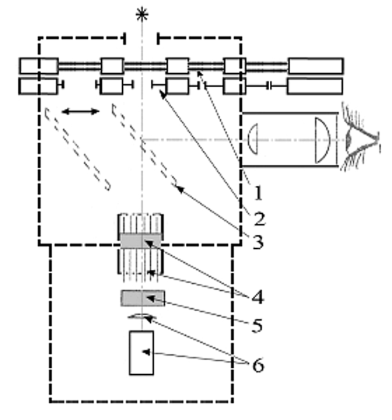
Figure 1: Block diagram of the single-channel photometer-polarimeter used in this work.

The observations were obtained using single-channel aperture photometer-polarimeter installed on the Cassegrain focus of the 2.6-m Shajn mirror telescope (SMT) at the Crimean astrophysical observatory (Ukraine). A rotating strained plexiglass quarter-wave plate calculated by Kucherov (1986) and developed by Samoilov & Samoilov (2015) was used as a circular polarization modulator. After the tests under laboratory conditions it turned out that optical efficiency of this plate is similar to quartz plates, but plexiglass is less sensitive to temperature changes. The retarder plate is continuously rotating at the rate of 33 rps. It allows us to measure circular and linear polarization simultaneously. Optical system of the polatimeter is presented at the Fig. 1. It consists of the:

1. filter wheel

2. aperture

3. mobile mirror

4. the quarter-wave plate rotating at the rate of 33 rps

5. Glan prism (analyzer)

6. photomultiplier tube with the Fabry lens

Detailed description of the instrument was presented by Kolesnikov et al. (2016).

The possibility of linear to circular cross-talk in the instrument was studied in laboratory conditions: the maximal value was found to be 1.5

We used mostly WR (Wide-R, 550-750 nm) and Johnson V and R filters. Few measurements were made using B and U flters. The typical object exposures are 1-10 seconds that depends on the target’s brightness and rate of variability. It allows us to study fast changes of each parameter or obtain smaller time resolution but higher accuracy by averaging. The whole data set contains about 1000 time series of different objects in 105 sets of observations between September 2002 and November 2017. Hereafter the set of observations is the period between the installation and removing of the polarimeter from the telescope (usually 1 to 5 consecutive nights).

3 Data processing

The intensity of light transmitted through a retarder with a quarter wave plate is described by the formula 1, where $I$, $Q$, $U$, $V$ - Stokes parameters, $\psi$ is the angle of rotation of the retarder axis relative to the analyzer principal plane (Serkowski 1974).

$$I=\frac{1}{2}\left(I\pm\frac{1}{2}Q\pm\frac{1}{2}Q\cos 4\psi\pm\frac{1}{2}U\sin 4\psi\mp V\sin 2\psi\right)$$ (1)

After angular integration of this equation for eight pulse counters (22.5 degrees each) and taking into account repeating after 180 degrees, 8 equations could be obtained (see Kolesnikov et al. 2016). These data is accumulated in 8 counters of the controller and stored for each exposure. To eliminate the background, series of target were alternated with series of background and series of comparison star to obtain photometry.

The background was fit by polynomials and subtracted from the data for each of 8 channels independently. Due to the fast rotation of the phase plate, we can exclude influence of majority of atmospheric phenomena. Twilight sky is characterized by rapid change of the background level, so the background series were made more frequently and a proper fit required high order polynomials. Each normal night with good atmospheric conditions shows slow background variations and absence of background polarization, so most of backgrounds were fitted using 0 or 1st order polynomials. Clouds or haze sometimes were linearly polarized, sometimes were not. We noticed that in the second case, partial haze or clouds were obviously harmful for photometry, but did not change the polarization, only increased dispersion was observed. So, if continuous series of particular target is highly important and the data loss is critical, it is possible to use data obtained using this type of instrument even through significant cloudiness. However, we excluded all suspicious points from the analysis of standards.

Contrary to classic algorithm used earlier (Breus et al. (2007); Kolesnikov et al. (2016)), based on determination of Stokes parameters from linear combinations of 8 equations, we used least squares approach. This way we get some benefits:

1. we can obtain all four Stokes parameters $I$, $Q$, $U$, $V$ and their accuracies using trivial formulas

2. we do not need to determine a position angle of circular polarization diagram using objects with high-amplitude variability of circular polarization, to obtain circular polarization degree from $CP1$ and $CP2$

3. we stop neglecting influence of non-zero $Q$ on $I$, valid only for signal with low values of $Q$

4. the accuracy of the results obtained using this approach is obviously better.

Also we may exclude the influence of artificial noise or electrical interference in conductors by excluding up to 4 erroneous channels (with decrease of the results accuracy). As interference happened irregularly and could not be predicted, detection of interference was implemented using complicated algorithm based on analysis of moving average in each of 8 channels. Normalized Stokes parameters were calculated as follows:

$$q=\frac{Q}{I},u=\frac{U}{I},v=\frac{V}{I}$$ (2)

The total linear polarization

$$p=\sqrt[]{q^{2}+u^{2}}$$ (3)

Throughout this work, the normalized Stokes parameters $q$, $u$, $v$ and linear polarization degree $p$ are given in per cents, position angle $\theta$ is given in degrees. All measurements of $\theta$ are referred to equatorial coordinates.

Measurements of zero-polarization stars are used for computation of the instrumental polarization. Classic approach implies usage of the measurements obtained each night before and/or after the observations, in the same filter, similarly to the flat field and dark frames in CCD photometry. Usually the mean values of normalized Stokes parameters over the observations set were used (one set is a time interval that consist of a few days up to one week of continuous observations without dismantling the equipment). We found that these mean values are not statistically different from set to set. We noticed different behaviour, which clearly separated the period before replacing the reflective layer of the main mirror of the telescope and after it. It was originally detected with the dependency of linear polarization degree on time, but later determined for normalized Stokes parameters q and u separately. For example, at the first (flat) interval, $q=0.026(10)\%$, $u=0.036(12)\%$, so the magnitude of the instrumental polarization is not negligible. The difference of fits of instrumental polarization obtained for WR, R, V and B filters is not statistically significant, so we used all measurements together. Thus the instrumental polarization was determined in the form of piecewise continuous functions from the observations of about 65 non-polarized stars for the whole data interval. Subtracting these values from the normalized Stokes parameters we eliminate the instrumental linear polarization. In each set, few different highly polarization standards were observed for calibration of position angle zero-point. We checked that the difference between position angle in our instrumental system and the catalog value for the corresponding star (Heiles (2000); Leroy (1993)) was constant during each set of observations for absolute majority of standards. Contrary to the classic approach, where the position angle was determined for each set of observations, taking into account statistically insignificant difference between many consecutive sets, we decided to determine the position angle for larger time intervals. Weighted mean values of the difference were calculated. Here and later we used the weight inversely proportional to the square of the error estimate of the value. Summarizing, about one third of all data set time interval had the same position angle value, one third had another value, and the rest of the data (the earliest years) show position angle changes from set to set due to changes of the device. We have rotated the axes $Q$, $U$ on these angles to align our measurements to equatorial coordinates. Thus, the weighted mean values of the instrumental linear polarization and position angle were determined using significantly larger number of observations (few sets instead of one) and obviously are more accurate than determined earlier by few measurements of standard stars during one or two consequent sets. After the correction for background and instrumental polarization, the intensity $I$ and normalized Stokes parameters $q$, $u$, $v$ with its error estimates are stored in the form of time series and are subject for further analysis. For the constant objects (like polarization standards and zero-polarization stars) we used weighted mean of Stokes parameters for each run. The errors were computed as the standard errors of the weighted mean values.

$$\theta=0.5\arctan\frac{u}{q}$$ (4)

$$\sigma\left(p\right)=\sqrt[]{\sigma\left(q\right)^{2}+\sigma\left(u\right)^{2}}$$

$$\sigma\left(\theta\right)=\arctan\frac{0.5\sigma\left(p\right)}{p}$$

The final values of each Stokes parameter were obtained as follows: the weighted mean value and its standard error were calculated for each object during the first iteration. Then we excluded all runs, that deviates from the mean value for more then $2\sigma$ and repeated the calculation of weighted mean and the error. The linear polarization degree, the position angle and their error estimates were calculated from the final values of Q and U using Formula 4.

These results are shown as normalized Stokes parameters in the Table 1.

Table 1: Results of standard polarized and unpolarized stars. From the left to the right are given: object name, band, number of different nights, total number of exposures, sum of exposure durations in minutes, normalized Stokes parameters q, u, v, the linear polarization degree in percents and the position angle referred to equatorial coordinates with their error estimates.

Object	Filter	N	NP	$\delta$T, min	q	$\sigma$q	u	$\sigma$u	v	$\sigma$v	p	$\sigma$p	$\theta$	$\sigma\theta$
BD+332642	V	1	512	54	0.168	0.045	0.059	0.045	0.001	0.020	0.178	0.063	99.6	10.0
BD+332642	WR	6	1708	161	-0.039	0.018	0.089	0.018	-0.001	0.008	0.097	0.025	146.9	7.3
BD+64 106	V	2	632	51	5.415	0.044	1.382	0.043	0.028	0.021	5.589	0.061	97.2	0.3
BD+64 106	WR	2	352	26	5.261	0.040	1.550	0.039	0.008	0.018	5.485	0.055	98.2	0.3
BD284211	V	4	1069	80	0.605	0.026	-0.298	0.026	-0.014	0.012	0.674	0.037	76.9	1.6
BD284211	WR	4	734	94	-0.005	0.027	0.050	0.027	-0.041	0.012	0.050	0.037	138.1	20.6
G191B2B	V	1	600	44	-0.303	0.088	0.336	0.088	0.217	0.041	0.453	0.125	156.0	7.9
G191B2B	WR	3	628	89	0.025	0.028	0.244	0.028	0.003	0.013	0.246	0.040	132.1	4.6
HD102870	R	1	512	36	-0.023	0.011	-0.063	0.011	0.049	0.005	0.067	0.016	35.2	6.9
HD102870	WR	6	1102	90	-0.040	0.002	0.012	0.002	-0.013	0.001	0.042	0.003	171.9	1.9
HD103095	WR	1	320	24	-0.066	0.017	0.055	0.017	0.030	0.008	0.086	0.024	160.1	8.1
HD10476	R	3	1600	114	-0.015	0.005	-0.073	0.005	0.030	0.002	0.075	0.007	39.1	2.8
HD10476	WR	8	1344	84	0.021	0.003	0.029	0.003	0.054	0.001	0.036	0.004	116.9	3.4
HD10898	R	1	283	19	3.454	0.047	0.316	0.047	0.070	0.022	3.468	0.067	92.6	0.6
HD10898	V	1	703	54	4.244	0.022	0.374	0.021	-0.002	0.010	4.260	0.030	92.5	0.2
HD10898	WR	1	80	14	3.561	0.049	0.755	0.048	0.000	0.022	3.640	0.068	96.0	0.5
HD109358	WR	7	1601	133	-0.003	0.002	0.024	0.002	0.046	0.001	0.024	0.003	138.2	3.8
HD110897	WR	2	494	35	-0.018	0.008	0.011	0.008	-0.011	0.004	0.021	0.011	164.4	15.5
HD111395	R	1	84	18	-0.064	0.072	-0.229	0.073	-0.057	0.033	0.238	0.102	37.2	12.1
HD114710	R	1	512	36	-0.061	0.014	-0.027	0.014	0.020	0.006	0.066	0.019	12.2	8.3
HD114710	WR	12	2767	208	-0.053	0.001	0.007	0.001	0.000	0.001	0.053	0.002	176.1	1.1
HD125184	WR	2	1280	92	-0.151	0.008	-0.037	0.008	0.035	0.004	0.156	0.011	6.8	2.1
HD126660	WR	5	966	61	-0.007	0.002	-0.012	0.002	0.011	0.001	0.014	0.003	29.8	6.4
HD127665	WR	3	576	57	-0.035	0.009	0.348	0.009	0.016	0.004	0.350	0.012	137.9	1.0
HD127762	WR	9	1216	96	-0.020	0.001	-0.044	0.001	0.016	0.001	0.049	0.002	32.6	1.2
HD14069	R	1	640	46	-0.031	0.011	-0.082	0.011	0.147	0.005	0.087	0.016	34.6	5.1
HD14069	V	6	2767	171	0.295	0.014	0.153	0.014	-0.072	0.006	0.332	0.020	103.7	1.7
HD14069	WR	7	2344	127	0.052	0.004	-0.005	0.004	0.078	0.002	0.052	0.006	87.3	3.2
HD142373	WR	2	192	14	0.026	0.006	-0.046	0.006	0.007	0.003	0.052	0.008	59.7	4.4
HD144287	B	1	62	12	-0.153	0.251	0.042	0.250	-0.047	0.116	0.158	0.354	172.3	48.2
HD144287	R	1	576	46	0.011	0.030	0.111	0.030	0.060	0.014	0.111	0.043	132.3	10.9
HD144287	V	3	632	65	0.013	0.016	-0.003	0.016	0.046	0.007	0.014	0.022	84.1	39.1
HD144287	WR	8	1912	165	0.063	0.008	0.021	0.008	0.030	0.003	0.067	0.011	99.3	4.6
HD14433	B	1	78	20	2.144	1.061	2.961	1.060	0.082	0.497	3.656	1.500	117.0	11.6
HD14433	V	2	87	19	2.615	0.099	2.801	0.099	-0.069	0.046	3.832	0.139	113.5	1.0
HD14433	WR	3	396	35	2.321	0.062	2.587	0.063	-0.041	0.029	3.475	0.088	114.1	0.7
HD144579	R	1	160	12	-0.018	0.018	-0.093	0.018	0.082	0.008	0.095	0.026	39.5	7.7
HD144579	V	1	60	10	-0.057	0.063	0.059	0.063	-0.036	0.029	0.082	0.089	157.0	28.5
HD144579	WR	2	120	20	-0.226	0.046	-0.057	0.046	-0.023	0.021	0.233	0.065	7.1	8.0
HD146233	V	1	128	9	0.017	0.024	0.063	0.024	-0.088	0.011	0.065	0.034	127.5	14.7
HD146233	WR	2	504	102	0.271	0.006	-0.030	0.006	0.022	0.003	0.273	0.009	86.8	0.9
HD15089	WR	3	640	70	-0.258	0.011	-0.002	0.011	-0.080	0.005	0.258	0.015	0.2	1.7
HD154345	B	1	80	15	0.034	0.049	-0.043	0.049	0.035	0.023	0.055	0.069	63.9	32.2
HD154345	R	3	640	72	-0.107	0.032	0.070	0.032	-0.072	0.015	0.128	0.046	163.3	10.1
HD154345	V	6	700	136	0.008	0.017	0.015	0.017	-0.034	0.008	0.017	0.024	120.5	34.6
HD154345	WR	15	2415	300	0.044	0.005	-0.060	0.005	0.000	0.002	0.074	0.007	63.1	2.7
HD154892	R	1	640	47	-0.072	0.044	0.005	0.044	0.077	0.020	0.072	0.062	178.0	23.3
HD154892	V	2	640	46	0.085	0.018	-0.064	0.018	0.075	0.008	0.106	0.025	71.6	6.8
HD154892	WR	8	1589	117	0.050	0.008	-0.036	0.008	-0.007	0.004	0.062	0.011	71.9	5.2
HD155528	V	1	511	37	5.210	0.047	0.278	0.047	0.105	0.022	5.217	0.067	91.5	0.4
HD155528	WR	2	96	6	4.567	0.059	-0.853	0.060	0.092	0.028	4.646	0.084	84.7	0.5
HD157214	V	2	256	17	0.034	0.010	-0.078	0.010	-0.072	0.004	0.085	0.014	56.6	4.6
HD157214	WR	4	320	22	0.049	0.006	0.117	0.006	0.004	0.003	0.127	0.008	123.6	1.8
HD165908	V	2	192	14	-0.025	0.008	-0.057	0.008	-0.026	0.003	0.062	0.011	33.0	4.9
HD165908	WR	9	1376	111	0.001	0.003	0.019	0.003	0.005	0.001	0.019	0.004	133.5	5.8
HD182572	WR	3	800	64	0.111	0.004	0.010	0.004	-0.017	0.002	0.112	0.006	92.5	1.5
HD185395	WR	3	448	33	0.053	0.006	0.037	0.006	-0.036	0.003	0.065	0.009	107.4	3.8
HD187929	WR	3	352	31	1.370	0.005	-0.074	0.005	0.019	0.002	1.372	0.007	88.5	0.1
HD18803	R	2	1019	86	0.001	0.015	-0.023	0.015	0.019	0.007	0.023	0.021	45.6	24.7
HD18803	WR	6	965	176	0.068	0.010	0.062	0.010	-0.009	0.004	0.092	0.014	111.3	4.3

Table 2: Continuation of the Table 1

Object	Filter	N	NP	$\delta$T, min	q	$\sigma$q	u	$\sigma$u	v	$\sigma$v	p	$\sigma$p	$\theta$	$\sigma\theta$
HD188326	B	3	796	80	0.295	0.027	0.112	0.027	0.144	0.012	0.315	0.038	100.4	3.5
HD188326	R	4	1864	162	0.013	0.012	-0.104	0.012	0.023	0.005	0.105	0.017	48.5	4.6
HD188326	V	4	554	65	0.114	0.020	-0.079	0.020	0.009	0.009	0.139	0.028	72.6	5.8
HD188326	WR	8	835	114	-0.001	0.009	-0.045	0.009	0.017	0.004	0.045	0.013	44.1	8.2
HD188512	V	1	64	4	-0.045	0.008	-0.010	0.008	-0.040	0.003	0.046	0.011	6.2	6.7
HD188512	WR	5	577	52	0.013	0.003	-0.022	0.003	-0.005	0.002	0.026	0.005	60.2	5.4
HD18883	WR	1	121	12	-0.013	0.036	-0.079	0.036	-0.039	0.016	0.080	0.050	40.5	17.4
HD190406	R	1	576	41	0.047	0.022	-0.033	0.022	0.145	0.010	0.057	0.031	72.6	15.3
HD190406	WR	3	544	39	0.014	0.006	0.047	0.006	0.092	0.003	0.049	0.009	126.8	5.2
HD191854	R	1	1400	101	0.054	0.023	-0.043	0.023	0.065	0.011	0.069	0.033	70.9	13.5
HD191854	WR	1	770	60	-0.021	0.011	-0.060	0.011	-0.027	0.005	0.063	0.015	35.2	6.8
HD193092	WR	1	128	9	-0.004	0.010	0.069	0.010	0.067	0.004	0.069	0.014	136.5	5.8
HD193426	V	1	128	10	0.143	0.059	1.868	0.058	0.015	0.027	1.874	0.083	132.8	1.3
HD193426	WR	1	32	2	-0.221	0.316	0.413	0.315	-0.227	0.148	0.469	0.446	149.0	25.5
HD193487	WR	1	256	19	-0.039	0.016	-0.157	0.016	-0.001	0.007	0.162	0.023	38.1	4.0
HD19373	B	1	256	19	-0.096	0.006	0.231	0.006	0.085	0.003	0.250	0.008	146.3	1.0
HD19373	R	1	256	18	-0.011	0.014	0.044	0.014	-0.005	0.006	0.045	0.019	142.0	12.0
HD19373	V	1	192	14	0.004	0.006	-0.099	0.006	-0.017	0.003	0.100	0.008	46.1	2.4
HD19373	WR	2	320	24	-0.029	0.004	-0.011	0.004	-0.013	0.002	0.031	0.005	10.5	4.7
HD195068	WR	2	506	59	-0.009	0.006	-0.019	0.006	0.077	0.003	0.021	0.008	33.0	10.8
HD196850	R	1	768	56	-0.310	0.018	-0.029	0.018	-0.067	0.008	0.312	0.026	2.7	2.4
HD196850	WR	1	384	28	-0.004	0.010	-0.025	0.010	0.016	0.005	0.026	0.014	41.0	15.5
HD198149	WR	2	384	44	0.012	0.002	-0.002	0.002	-0.019	0.001	0.012	0.003	86.2	7.2
HD19820	V	1	170	14	3.121	0.041	3.670	0.040	0.055	0.019	4.817	0.057	114.8	0.3
HD19820	WR	2	144	10	2.613	0.019	3.027	0.019	-0.019	0.009	3.998	0.027	114.6	0.2
HD198478	R	1	320	22	-1.862	0.033	-0.425	0.033	0.023	0.015	1.910	0.046	6.4	0.7
HD198478	V	4	596	79	-2.638	0.012	-0.089	0.012	-0.021	0.006	2.639	0.017	1.0	0.2
HD198478	WR	8	1519	117	-2.027	0.004	0.028	0.004	-0.031	0.002	2.027	0.006	179.6	0.1
HD199100	WR	2	832	94	0.138	0.012	-0.130	0.012	0.002	0.005	0.190	0.017	68.3	2.5
HD200077	WR	4	825	59	-0.037	0.006	0.054	0.006	0.053	0.003	0.066	0.008	152.2	3.4
HD20630	R	1	476	40	0.021	0.020	-0.121	0.020	0.077	0.009	0.123	0.028	49.8	6.6
HD20630	WR	1	128	9	-0.072	0.006	-0.028	0.006	0.037	0.003	0.078	0.009	10.7	3.4
HD210027	B	1	192	15	0.040	0.007	0.216	0.007	0.109	0.003	0.220	0.009	129.7	1.2
HD210027	R	1	320	25	0.074	0.012	-0.037	0.012	0.050	0.005	0.083	0.017	76.7	5.8
HD210027	V	2	318	23	-0.030	0.005	-0.009	0.005	-0.053	0.002	0.032	0.007	8.6	6.3
HD210027	WR	7	1116	84	-0.002	0.002	-0.034	0.002	0.019	0.001	0.034	0.003	43.1	2.4
HD212311	R	1	192	29	0.159	0.078	0.160	0.078	-0.121	0.036	0.225	0.110	112.6	13.8
HD212311	V	1	576	43	-0.011	0.018	-0.132	0.018	-0.166	0.008	0.133	0.025	42.5	5.5
HD21447	WR	2	376	30	-0.242	0.006	0.020	0.006	-0.015	0.003	0.243	0.008	177.7	1.0
HD214923	B	1	256	24	-0.009	0.004	0.001	0.004	0.002	0.002	0.009	0.005	175.9	15.8
HD214923	R	2	768	58	-0.022	0.009	0.016	0.009	-0.033	0.004	0.027	0.013	162.2	13.1
HD214923	V	1	128	9	-0.061	0.012	-0.007	0.012	-0.139	0.005	0.061	0.017	3.3	8.1
HD214923	WR	5	564	50	-0.029	0.003	-0.002	0.003	0.002	0.001	0.029	0.004	1.6	3.6
HD216228	WR	2	608	51	-0.003	0.005	0.003	0.005	-0.045	0.002	0.004	0.007	158.5	44.4
HD216411	B	1	60	11	-0.031	0.318	-2.482	0.318	-0.094	0.146	2.483	0.450	44.6	5.2
HD216411	V	1	40	6	0.047	0.402	-2.841	0.402	-0.016	0.184	2.842	0.569	45.5	5.7
HD216411	WR	1	272	20	-0.444	0.019	-2.723	0.019	-0.032	0.009	2.759	0.027	40.4	0.3
HD21770	R	1	640	43	0.053	0.015	-0.026	0.015	-0.027	0.007	0.059	0.022	76.8	10.4
HD222107	R	1	192	13	-0.072	0.113	0.339	0.113	-0.011	0.052	0.346	0.159	141.0	13.0
HD222107	WR	1	740	68	-0.176	0.015	-0.052	0.015	-0.031	0.007	0.183	0.022	8.2	3.4
HD23512	R	1	128	9	1.314	0.138	2.307	0.137	-0.001	0.064	2.655	0.195	120.2	2.1
HD23512	WR	2	384	28	-1.373	0.021	-1.564	0.021	0.073	0.010	2.081	0.030	24.4	0.4
HD251204	R	1	210	34	-0.847	0.081	2.319	0.080	-0.027	0.037	2.469	0.114	145.0	1.3
HD251204	V	3	1296	100	-2.790	0.029	3.912	0.028	0.060	0.013	4.805	0.040	152.7	0.2
HD251204	WR	1	80	23	-2.612	0.312	4.093	0.319	-0.011	0.144	4.856	0.447	151.3	2.6
HD257971	WR	1	704	57	-0.096	0.019	-0.006	0.019	0.001	0.009	0.096	0.027	1.7	7.9
HD25914	B	1	22	4	-0.961	0.065	4.771	0.067	0.027	0.030	4.867	0.093	140.7	0.5
HD25914	V	2	328	25	-0.786	0.023	4.394	0.022	0.027	0.010	4.464	0.032	140.1	0.2
HD25914	WR	5	425	47	-0.502	0.023	4.395	0.023	0.002	0.011	4.424	0.032	138.3	0.2
HD34411	R	1	576	41	-0.055	0.013	-0.103	0.013	0.069	0.006	0.117	0.019	30.8	4.6
HD34411	WR	2	128	9	-0.001	0.007	0.037	0.007	0.072	0.003	0.037	0.011	135.5	8.1
HD39587	WR	2	256	18	0.073	0.005	-0.053	0.005	0.021	0.002	0.090	0.008	72.0	2.4

Table 3: Continuation of the Table 1

Object	Filter	N	NP	$\delta$T, min	q	$\sigma$q	u	$\sigma$u	v	$\sigma$v	p	$\sigma$p	$\theta$	$\sigma\theta$
HD41398	V	1	320	27	-2.119	0.026	1.145	0.026	0.062	0.012	2.408	0.037	165.8	0.4
HD42618	R	1	640	50	0.085	0.013	-0.002	0.013	-0.028	0.006	0.085	0.018	89.2	5.9
HD42618	WR	1	80	16	-0.071	0.035	0.143	0.035	-0.010	0.016	0.160	0.049	148.3	8.7
HD432	R	3	612	58	-0.009	0.006	-0.027	0.006	0.071	0.003	0.029	0.008	35.5	8.1
HD432	WR	7	752	67	-0.066	0.002	-0.054	0.002	-0.010	0.001	0.085	0.003	19.5	0.9
HD43384	R	5	1504	113	-2.012	0.009	0.854	0.009	0.004	0.004	2.186	0.012	168.5	0.2
HD43384	WR	6	1051	95	-2.285	0.007	0.747	0.007	0.031	0.003	2.404	0.010	170.9	0.1
HD50019	R	2	1397	126	-0.005	0.009	-0.044	0.009	0.000	0.004	0.045	0.013	41.7	8.1
HD50019	WR	1	95	7	0.054	0.011	0.060	0.011	0.081	0.005	0.081	0.015	114.1	5.3
HD50973	WR	1	320	22	0.008	0.006	0.061	0.006	0.043	0.003	0.062	0.009	131.1	4.1
HD57702	WR	1	128	9	-0.014	0.030	0.035	0.030	-0.024	0.014	0.037	0.042	145.7	29.5
HD65583	R	5	2580	199	0.033	0.010	0.016	0.010	0.004	0.004	0.036	0.014	103.4	10.6
HD65583	V	3	864	66	0.046	0.013	0.022	0.014	0.051	0.006	0.051	0.019	102.5	10.6
HD65583	WR	23	7027	722	0.011	0.003	-0.004	0.003	0.026	0.002	0.012	0.005	80.2	11.2
HD7927	R	1	224	16	1.812	0.006	0.092	0.006	-0.003	0.003	1.814	0.008	91.5	0.1
HD7927	WR	5	1328	156	2.669	0.010	-0.030	0.010	0.012	0.005	2.669	0.014	89.7	0.1
HD82885	R	3	2055	149	0.053	0.008	-0.043	0.008	0.019	0.004	0.068	0.011	70.4	4.8
HD82885	WR	2	448	32	-0.031	0.004	0.004	0.004	0.000	0.002	0.031	0.005	176.2	5.0
HD90508	R	2	959	74	-0.114	0.016	-0.011	0.016	-0.055	0.007	0.114	0.022	2.8	5.6
HD90508	WR	3	896	63	-0.026	0.005	0.014	0.005	0.005	0.002	0.030	0.007	166.1	7.1
HD9407	V	1	80	17	-0.215	0.069	0.085	0.069	0.133	0.032	0.231	0.097	169.2	11.9
HD9407	WR	1	262	23	0.133	0.013	-0.043	0.013	-0.033	0.006	0.140	0.019	81.0	3.8
HD95418	R	1	192	14	-0.089	0.018	-0.079	0.018	0.114	0.008	0.119	0.025	20.8	6.0
HD95418	WR	1	128	9	0.000	0.012	0.174	0.012	0.032	0.005	0.174	0.018	135.0	2.9
HD98281	WR	1	384	29	0.002	0.012	-0.012	0.012	-0.002	0.005	0.012	0.017	49.1	34.7
HILTNER 960	V	2	512	39	0.938	0.044	-5.314	0.045	-0.024	0.021	5.396	0.063	50.0	0.3
HILTNER 960	WR	3	435	57	1.731	0.024	-5.155	0.024	0.023	0.011	5.438	0.034	54.3	0.2
Object	Filter	N	NP	$\delta$T, min	Q	$\sigma$Q	U	$\sigma$U	V	$\sigma$V	P	$\sigma$P	$\theta$	$\sigma\theta$
GD319	V	1	584	48	0.794	0.118	0.162	0.119	0.477	0.054	0.811	0.167	95.8	5.9
GD319	WR	3	2700	227	-0.133	0.033	0.111	0.033	-0.019	0.015	0.173	0.046	160.0	7.6
HD154445	V	1	128	9	3.827	0.072	0.355	0.074	-0.015	0.032	3.844	0.104	92.7	0.8
HD154445	WR	7	1023	82	2.730	0.006	-0.106	0.006	0.055	0.003	2.732	0.008	88.9	0.1
HD155197	R	1	640	111	3.651	0.093	1.708	0.092	-0.077	0.043	4.031	0.131	102.5	0.9
HD155197	V	5	1091	112	4.089	0.023	1.981	0.022	0.025	0.011	4.543	0.032	102.9	0.2
HD155197	WR	5	899	74	2.355	0.018	1.689	0.018	0.021	0.008	2.898	0.025	107.8	0.3
HD183143	B	3	902	73	-5.926	0.025	0.255	0.024	0.091	0.011	5.932	0.035	178.8	0.2
HD183143	R	4	808	72	-5.632	0.019	0.581	0.019	0.042	0.009	5.662	0.027	177.1	0.1
HD183143	V	4	689	60	-5.809	0.014	0.425	0.014	0.051	0.006	5.824	0.020	177.9	0.1
HD183143	WR	5	716	72	-5.667	0.008	-0.102	0.008	0.084	0.004	5.668	0.012	0.5	0.1
HD204827	B	1	20	3	-0.107	0.383	0.483	0.383	-0.032	0.177	0.495	0.542	141.2	28.7
HD204827	R	1	48	10	-0.210	0.196	-3.741	0.200	-0.309	0.092	3.747	0.280	43.4	2.1
HD204827	V	4	598	59	2.619	0.016	-4.944	0.016	0.012	0.008	5.595	0.023	59.0	0.1
HD204827	WR	9	1241	131	1.721	0.009	-3.412	0.009	-0.004	0.004	3.822	0.012	58.4	0.1
HD212311	WR	5	1805	165	0.579	0.008	0.113	0.008	-0.012	0.004	0.590	0.012	95.5	0.6
HD21291	WR	2	194	13	1.052	0.007	0.298	0.007	-0.033	0.003	1.093	0.009	97.9	0.2
HD236928	V	3	860	51	6.755	0.023	1.737	0.024	-0.092	0.011	6.975	0.033	97.2	0.1
HD236928	WR	5	912	87	2.585	0.018	1.364	0.018	-0.039	0.008	2.923	0.025	103.9	0.2
HD236954	WR	1	320	24	5.489	0.181	1.882	0.179	-0.122	0.085	5.803	0.255	99.5	1.3
HD331891	R	2	544	11	0.618	0.082	0.307	0.082	0.070	0.038	0.689	0.116	103.2	4.8
HD331891	V	5	1791	81	0.186	0.017	-0.116	0.017	0.035	0.008	0.219	0.023	74.1	3.1
HD331891	WR	7	2113	139	0.092	0.011	0.005	0.011	-0.012	0.005	0.092	0.016	91.7	5.0
Object	Filter	N	NP	$\delta$T, min	Q	$\sigma$Q	U	$\sigma$U	V	$\sigma$V	P	$\sigma$P	$\theta$	$\sigma\theta$
HD14489	R	4	1141	90	0.030	0.009	-0.014	0.009	0.026	0.004	0.034	0.012	77.5	10.2
HD14489	WR	1	256	20	0.113	0.027	0.365	0.027	0.018	0.012	0.383	0.038	126.4	2.9
HD177463	R	1	634	45	0.068	0.016	-0.037	0.016	-0.010	0.007	0.077	0.022	75.7	8.1
HD177463	WR	1	246	22	0.024	0.007	0.034	0.007	0.132	0.003	0.042	0.010	117.4	7.1
HD283812	R	1	100	12	-1.210	0.067	-3.816	0.069	-0.422	0.032	4.003	0.096	36.2	0.7
HD283812	V	5	2170	108	-2.506	0.021	-5.880	0.021	0.058	0.010	6.391	0.030	33.5	0.1
HD283812	WR	5	976	59	-2.632	0.022	-5.628	0.023	0.047	0.010	6.213	0.031	32.5	0.1
HD4768	R	1	736	55	1.741	0.028	-0.833	0.028	-0.112	0.013	1.930	0.039	77.2	0.6
HD161056	WR	2	448	36	2.633	0.011	2.546	0.012	0.150	0.005	3.662	0.016	112.0	0.1
HD147084	WR	1	128	10	-1.092	0.008	2.874	0.008	0.111	0.004	3.074	0.012	145.4	0.1
HD34282	WR	1	544	54	1.004	0.171	-2.486	0.325	0.946	0.147	2.681	0.305	56.0	1.9
HD163993	WR	2	192	15	-0.013	0.005	0.045	0.005	0.133	0.002	0.047	0.008	143.1	4.6
HD90839	R	1	271	20	-0.007	0.029	-0.098	0.029	0.079	0.013	0.099	0.040	42.9	11.6
HD90839	WR	1	256	19	0.011	0.005	0.044	0.005	-0.048	0.002	0.045	0.007	128.2	4.3

4 Linear and Circular Polarization

Fig. 2 shows a comparison of the mean weighted linear polarization degree $p$, obtained in this work, with measurements from Heiles (2000) for each band. These charts contain all objects from the Table 1.

Fig. 3 shows a similar comparison of the position angle $\theta$ for those objects where it is determined in both sources. The angle, ranging from 0 to 180 degrees, means that values near 0 and values near 180 are the same.

A good agreement allows us to compile all the measurements together regardless of the used filter and a season when the data were obtained for majority of tasks.

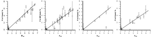
Figure 2: Dependence of the linear polarization degree for individual standards compiled for each band (from the left to the right B, V, WR, R) obtained in this work versus Heiles (2000) and corresponding linear fits.

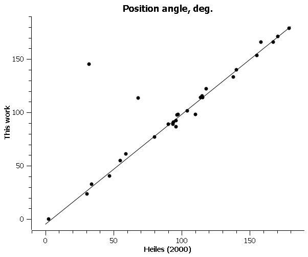
Figure 3: Dependence of the position angle for individual standards determined in this work versus Heiles (2000) and corresponding linear fit. Error bars are not presented since X axis data are compiled from different sources, some points have large Y axis formal error estimate despite the data is well consistent. Two outlying points have the error estimate of the same order as other points.

As one may see in the Table 1, for most objects the value of v, which corresponds to circular polarization, is not significant (i.e. less then 3 of its error estimate). Only 10 standard stars have statistically significant mean value of v, and 6 deserve special attention. The disagreement between linear polarization degrees from pair of sources for some standards up to few percent may happen due to different bandwidth, different filter, variability of the source, instability on interstellar clouds or other reasons. Objects, that have linear polarization or position angle significantly different from the catalog values, are also described below.

HD21447 shows polarization shows polarization degree $0.243(8)\%$ that is much higher then from Heiles (2000). Deb Roy et al. (2015) also obtained higher value of $0.13(4)\%$.

The polarization degree for HD154445 obtained in V is higher then in WR band ($3.84(10)\%$ and $2.732(8)\%$ respectively). It qualitatively confirms results obtained by different authors in V and R bands e.g. Schmidt et al. (1992) and Prasad et al. (2013). Bastien et al. (2007) mentioned that this object is variable because its difference is almost twice the limit set from the statistics.

HD14489 has the mean value of $P=0.07(19)\%$ for all data ($0.03(1)$ for R and $0.38(4)$ for WR band). At the same time, previous authors published the value of $2.17(20)\%$. The position angle values for WR are in a good agreement.

HD177463 shows the linear polarization degree of $0.055(59)\%$, averaged by 2 time series obtained in different years and different bands (WR and R), where individual values are in a good agreement with each other. At the same time, the catalog value is $0.42(4)\%$.

For HD283812 we obtained the polarization degree of $6.39(40)\%$, that is significantly different from the published $4.27(12)\%$. We obtained 11 time series for this object in different bands (V, R, WR) during 4 consequent years and the mean values for each set were higher then $6\%$, except one set that shows $4.04(70)\%$ that is shorter than others and show higher error estimate due to bad atmospheric conditions. Thus this set has lower weight and is not a reason to suspect the variability of this object.

For HD4768 we obtained only 1 run, that shows the linear polarization degree $1.93(4)\%$, that is statistically different from published $2.21(20)\%$. At the same time, this run is characterized by statistically significant circular polarization of $-0.112(13)\%$.

HD161056 was observed during 2 nights, in 2013 and 2017 in WR. The results of both time series are consistent. The degree of linear polarization is consistent with published by Heiles (2000), but the position angle is different: $68.2\pm 0.8$ (Heiles 2000) and $112.0\pm 0.1$ degrees (this work). This is an important issue, since this object is used as highly polarized standard for determination of position angle zero point by different authors. In both runs we see statistically significant low positive circular polarization about $0.15\%$. Bastien et al. (2007) classified this object as marginal (possible variable).

HD147084 shows similar results. We observed it during one night and obtained a linear polarization degree close to the published values, but with different polarization angle: $145.4(1)$ degrees (this work), $32.1(3)$ (Heiles 2000), $36.1$ in Schmid et al. (2018). Pavana et al. (2019) obtained few individual values ranged in $55.14-81.63$ degrees in their instrumental system during consequent nights, that corresponds to approximately $8?32$ degrees referred to equatorial coordinates. Their latest night $2455674.12$ has larger error estimate for p in B band, but the same in V band. It may argue for the same quality of data in V, but presence of the process which influences the polarization angle, not the degree. During our run this object showed circular polarization of $0.111(4)\%$. This object was supposed to be low-amplitude heavily-reddened star by Garrison (1967), but was not studied enough, so must not be used as a polarization standard.

HD34282 is a UXOR+DSCT variable star, which shows variable polarization. We obtained $V=0.95(15)\%$ and $P=2.68(0.31)\%$. It is listed in catalogue by Heiles 2000 with the value of $P=0.13(4)\%$, but must not be used as a polarization standard.

HD163993 was observed during 2 nights in consequent months of 2013. Both runs shows similar, relatively high and statistically significant circular polarization of $0.099(8)\%$ and $0.133(4)\%$, respectively.

HD90839 was observed during 2 nights in 2013 and 2014. The first run is characterized by small, but statistically significant circular and linear polarizations. The second run shows only linear polarization of $0.136(44)\%$. This object is known as a star with a debris disc (Vandeportal 2019) and a high proper-motion star (Simbad). Thus, polarized emission and the variability of the polarization could happen in this type of objects.

5 Discussion

5.1 Polarimetric system

We compared linear polarization degree p (percents) for common stars in the pairs of the data sources: Heiles (2000) versus our data. The data is well agreed, but we found that the linear fit depends on the band, thus we calculated weighted linear fits in the forms of $y=k(x-x_{0})+c$ and $y=kx+b$ for data obtained in each photometric filter independently. Here $x_{0}$ is the mean value of the x axis, that are published values of the linear polarization degree. The coefficients of the first one is presented in the Table 4.

We noticed that these fits are statistically different and this approach may be used not only for polarization scale calibration, but also for converting the results obtained using different photometric systems to one system similarly to how it is used to be in photometry.

Table 4: The coefficients of the weighted linear fit to dependence of linear polarization degree p for common stars in the pairs of the data sources.

Band	k	$\sigma k$	c	$\sigma c$	$x_{0}$	$\chi^{2}$
B	0.9564	0.1272	1.6240	0.2065	1.6460	112
R	0.8127	0.0238	0.8440	0.0237	0.9493	140
U	1.0215	0.1504	1.7339	0.2599	1.4258	42
V	1.1115	0.0079	2.2230	0.0152	1.9635	214
WR	0.8737	0.0041	0.9862	0.0058	1.0961	214

5.2 The Variability of Standard Stars

We built time series of each Stokes parameter of each standard star by each band separately for full time interval and analysed them using well known numerical parameters characterizing the degree of variability (so called variability indices). We chose scatter-based indices, that we used earlier for variability detection on photometric data (see Breus (2017), Breus (2019)): standard deviation, $\chi^{2}$ test, Median absolute deviation, Robust median statistic and Normalized excess variance. Also we used Welch test (see Clarke & Stewart (1986)) for all time series. We marked all time series where at least one variability detection index shows an outstanding value. All stars, that have at least one time series marked few times were moved to the penultimate section of the Table 1. These stars are suspected to exhibit variability of at least one Stokes parameter, so they should not be used as polarized standard stars without further investigation.

6 Conclusions

1. We re-determined values of Stokes parameters for 98 standard stars (both non-polarized and highly polarized) and presented them along with the polarization degree p in the tables. This catalogue is not compilative, but obtained using the same instrument and technique during large time interval. It will be used for our future research and it may be used by other authors.

2. We implemented the least squares approach for determination of the Stokes parameters. It allowed us to obtain results with better accuracy.

3. Due to the dependence of polarization degree on the bandwidth, the statistical dependencies may be used for calibration and converting the results obtained using different photopolarimetric systems to one system similarly to how it is used to be in photometry.

4. The determination of the position angle zero point should be done using at least 3 highly polarized standards to exclude possible errors. One of chosen standard stars may have a position angle which varies with wavelength (which suggests that there are multiple polarization components) or time (polarization component variability). Passing of polarized interstellar clouds may also temporary effect the observable position angle. Despite this is an obvious conclusion, some authors use only one or two standards.

5. The same is true for zero-polarization standards.

6. Usage of insufficiently explored standards is possible only for determination of the correct coordinate quarter or clarification of the mean values of instrumental polarization together with well known reliable standards. This approach will also increase the number of well known standards.

7. It is also not desirable to use only agglomeration catalogs.

8. Although Stokes parameters may have different statistical distribution, we adopted selected scatter-based indices widely used for analysis of photometric data and compared with Welch test. We obtained similar results that means these scatter-based indices may be used for detection of polarization variability and it was confirmed on large array of uniform data. We report suspicious or variable stars that should no longer be used as polarized standards to obtain precise results.

References

- Bastien et al. (2007) Bastien P., Vernet E., Drissen L., Ménard F., Moffat A. F. J., Robert C., St-Louis N., 2007, in Sterken C., ed., Astronomical Society of the Pacific Conference Series Vol. 364, The Future of Photometric, Spectrophotometric and Polarimetric Standardization. p. 529
- Breus (2007) Breus V. V., 2007, Odessa Astronomical Publications, \hrefhttps://ui.adsabs.harvard.edu/abs/2007OAP….20…32B 20, 32
- Breus (2017) Breus V. V., 2017, \hrefhttp://dx.doi.org/10.17721/2227-1481.7.3-5 Advances in Astronomy and Space Physics, \hrefhttps://ui.adsabs.harvard.edu/abs/2017AASP….7….3B 7, 3
- Breus (2019) Breus V. V., 2019, Open European Journal on Variable Stars, \hrefhttps://ui.adsabs.harvard.edu/abs/2019OEJV..197…61B 197, 61
- Breus et al. (2007) Breus V. V., Andronov I. L., Kolesnikov S. V., Shakhovskoy N. M., 2007, \hrefhttp://dx.doi.org/10.1080/10556790701243225 Astronomical and Astrophysical Transactions, \hrefhttps://ui.adsabs.harvard.edu/abs/2007A&AT…26..241B 26, 241
- Breus et al. (2013) Breus V. V., et al., 2013, Journal of Physical Studies, \hrefhttps://ui.adsabs.harvard.edu/abs/2013JPhSt..17.3901B 17, 3902
- Clarke & Stewart (1986) Clarke D., Stewart B. G., 1986, \hrefhttp://dx.doi.org/10.1016/0083-6656(86)90013-9 Vistas in Astronomy, \hrefhttps://ui.adsabs.harvard.edu/abs/1986VA…..29…27C 29, 27
- Deb Roy et al. (2015) Deb Roy P., Halder P., Das H. S., Medhi B. J., 2015, \hrefhttp://dx.doi.org/10.1093/mnras/stv707 MNRAS, \hrefhttps://ui.adsabs.harvard.edu/abs/2015MNRAS.450.1770D 450, 1770
- Efimov (1981) Efimov I. S., 1981, Izvestiya Ordena Trudovogo Krasnogo Znameni Krymskoj Astrofizicheskoj Observatorii, \hrefhttps://ui.adsabs.harvard.edu/abs/1981IzKry..63..118E 63, 118
- Garrison (1967) Garrison R. F., 1967, \hrefhttp://dx.doi.org/10.1086/149090 ApJ, \hrefhttps://ui.adsabs.harvard.edu/abs/1967ApJ…147.1003G 147, 1003
- Heiles (2000) Heiles C., 2000, \hrefhttp://dx.doi.org/10.1086/301236 AJ, \hrefhttps://ui.adsabs.harvard.edu/abs/2000AJ….119..923H 119, 923
- Kolesnikov (2019a) Kolesnikov S. V., 2019a, \hrefhttp://dx.doi.org/10.30970/jps.23.3901 Journal of Physical Studies, \hrefhttps://ui.adsabs.harvard.edu/abs/2019JPhSt..23.3901K 23, 3901
- Kolesnikov (2019b) Kolesnikov S. V., 2019b, \hrefhttp://dx.doi.org/10.30970/jps.23.4901 Journal of Physical Studies, \hrefhttps://ui.adsabs.harvard.edu/abs/2019JPhSt..23.4901K 23, 4901
- Kolesnikov et al. (2016) Kolesnikov S. V., Breus V. V., Kiselev N. N., Andronov I. L., 2016, \hrefhttp://dx.doi.org/10.18524/1810-4215.2016.29.85015 Odessa Astronomical Publications, \hrefhttps://ui.adsabs.harvard.edu/abs/2016OAP….29…74K 29, 74
- Kucherov (1986) Kucherov V. A., 1986, Kinematika i Fizika Nebesnykh Tel, \hrefhttps://ui.adsabs.harvard.edu/abs/1986KFNT….2…82K 2, 82
- Leroy (1993) Leroy J. L., 1993, A&AS, \hrefhttps://ui.adsabs.harvard.edu/abs/1993A&AS..101..551L 101, 551
- Mishchenko et al. (2010) Mishchenko M. I., et al., 2010, Polarimetric Remote Sensing of Solar System Objects
- Pavana et al. (2019) Pavana M., Anche R. M., Anupama G. C., Ramaprakash A. N., Selvakumar G., 2019, \hrefhttp://dx.doi.org/10.1051/0004-6361/201833728 A&A, \hrefhttps://ui.adsabs.harvard.edu/abs/2019A&A…622A.126P 622, A126
- Prasad et al. (2013) Prasad V., Pandey J. C., Patel M. K., Srivastava D. C., 2013, \hrefhttp://dx.doi.org/10.1016/j.newast.2012.10.001 New A, \hrefhttps://ui.adsabs.harvard.edu/abs/2013NewA…20…52P 20, 52
- Rosenbush et al. (2008) Rosenbush V., Kiselev N., Antoniuk K., Kolesnikov S., 2008, in Asteroids, Comets, Meteors 2008. p. 8393
- Schmid et al. (2018) Schmid H. M., et al., 2018, \hrefhttp://dx.doi.org/10.1051/0004-6361/201833620 A&A, \hrefhttps://ui.adsabs.harvard.edu/abs/2018A&A…619A…9S 619, A9
- Schmidt et al. (1992) Schmidt G. D., Elston R., Lupie O. L., 1992, \hrefhttp://dx.doi.org/10.1086/116341 AJ, \hrefhttps://ui.adsabs.harvard.edu/abs/1992AJ….104.1563S 104, 1563
- Serkowski (1974) Serkowski K., 1974, in Gehrels T., ed., IAU Colloq. 23: Planets, Stars, and Nebulae: Studied with Photopolarimetry. p. 135
- Shakhovskoj & Efimov (1972) Shakhovskoj N. M., Efimov Y. S., 1972, Izvestiya Ordena Trudovogo Krasnogo Znameni Krymskoj Astrofizicheskoj Observatorii, \hrefhttps://ui.adsabs.harvard.edu/abs/1972IzKry..45…90S 45, 90
- Shakhovskoj et al. (1998) Shakhovskoj N. M., Andronov I. L., Kolesnikov S. V., Khalevin A. V., 1998, Kinematics and Physics of Celestial Bodies, \hrefhttps://ui.adsabs.harvard.edu/abs/1998KPCB…14..359S 14, 359
- Shakhovskoy et al. (2001) Shakhovskoy N. M., Andronov I. L., Kolesnikov S. V., Khalevin A. V., 2001, Izvestiya Ordena Trudovogo Krasnogo Znameni Krymskoj Astrofizicheskoj Observatorii, \hrefhttps://ui.adsabs.harvard.edu/abs/2001IzKry..97…91S 97, 91
- Vandeportal et al. (2019) Vandeportal J., Bastien P., Simon A., Augereau J.-C., Storer É., 2019, \hrefhttp://dx.doi.org/10.1093/mnras/sty3060 MNRAS, \hrefhttps://ui.adsabs.harvard.edu/abs/2019MNRAS.483.3510V 483, 3510