The Massive and Distant Clusters of WISE Survey XI: Stellar Mass Fractions and Luminosity Functions of MaDCoWS Clusters at $z\sim 1$

Abstract

We present stellar mass fractions and composite luminosity functions (LFs) for a sample of 12 clusters from the Massive and Distant Clusters of WISE Survey (MaDCoWS) at a redshift range of $0.951\leq z\leq 1.43$. Using SED fitting of optical and deep mid-infrared photometry, we establish the membership of objects along the lines-of-sight to these clusters and calculate the stellar masses of member galaxies. We find stellar mass fractions for these clusters largely consistent with previous works, including appearing to display a negative correlation with total cluster mass. We measure a composite $3.6~{}\mathrm{\mu m}$ LF down to $m^{*}+2.5$ for all 12 clusters. Fitting a Schechter function to the LF, we find a characteristic $3.6~{}\mathrm{\mu m}$ magnitude of $m^{*}=19.83\pm 0.12$ and faint-end slope of $\alpha=-0.81\pm 0.10$ for the full sample at a mean redshift of $\bar{z}=1.18$. We also divide the clusters into high- and low-redshift bins at $\bar{z}=1.29$ and $\bar{z}=1.06$ respectively and measure a composite LF for each bin. We see a small, but statistically significant evolution in $m^{*}$ and $\alpha$—consistent with passive evolution—when we study the joint fit to the two parameters, which is probing the evolution of faint cluster galaxies at $z\sim 1$. This highlights the importance of deep IR data in studying the evolution of cluster galaxy populations at high-redshift.

1 Introduction

The evolution of galaxies in clusters both influences and is influenced by the partitioning of baryons between the stars in galaxies and the hot gas of the intracluster medium (ICM). The stellar mass fraction of a cluster—that is, the fraction of the total mass in stars—$f_{\star}$, offers an in situ measurement of this partitioning. Measuring $f_{\star}$ and its relation to other cluster properties can give insight into the feedback processes that drive the cycling of baryons between states and which affect how galaxies grow and evolve (e.g., Lin et al., 2003; Ettori et al., 2006; Conroy et al., 2007). In addition, the shape of the cluster luminosity function (LF) offers insight into the mass-assembly history of the cluster. The near-infrared (NIR) LF is a useful proxy for the stellar mass function, as the luminosity in those bands is tightly correlated with stellar mass. The NIR LF parameters and how they evolve over time therefore reflect the mass-assembly history of galaxies in the cluster (Kauffmann & Charlot, 1998).

Previous studies such as Gonzalez et al. (2013) have analyzed the trend of $f_{\star}$ with total cluster mass at $z\sim 0.1$ and found an anti-correlation. This suggests that in the local universe, larger clusters retain their gas better and are less efficient at forming stars. In Decker et al. (2019), we also studied the trend of $f_{\star}$ with cluster mass for a sample of infrared-selected clusters at high redshift and compared this to a sample of ICM-selected clusters at comparable redshifts to look for differences due to selection. While we found a larger scatter in $f_{\star}$ in the ICM-selected clusters, there was no significant offset between the two samples. We also measured a relationship between $f_{\star}$ and total mass that was consistent with that found by Gonzalez et al. (2013), but the scatter and systematic uncertainties were too high to draw firm conclusions.

Cluster LFs follow a Schechter distribution (Schechter, 1976) of the form

$$\Phi(m)=\frac{\ln(10)}{2.5}\Phi^{*}10^{-0.4(m-m^{*})(\alpha+1)}\mathrm{exp}(-10^{-0.4(m-m^{*})})$$

where the overall scaling is paramaterized as $\Phi^{*}$, the characteristic magnitude ‘knee’ at the bright end is parameterized as $m^{*}$ and the slope of the faint-end of the function is parameterized as $\alpha$. Many studies have examined the rest-frame NIR LF of galaxy clusters (e.g., de Propris et al., 1999; Strazzullo et al., 2006; Muzzin et al., 2007; Mancone et al., 2012; Wylezalek et al., 2014; Chan et al., 2019) to measure the characteristic magnitude of the cluster LF at different redshifts. However, measuring $m^{*}$ becomes more difficult at high-redshift because there is a strong degeneracy between $m^{*}$ and $\alpha$. Therefore meaningfully measuring the former at high-redshift requires increasingly deep mid-infrared data to also constrain the latter. Indeed, few previous studies have measured the NIR LF for all cluster members (i.e., those both on and off the red-sequence) at $z>1$ down to a depth sufficient to jointly fit both $m^{*}$ and $\alpha$.

To address these problems, we measure stellar mass fractions and LFs for a sample of clusters from the Massive and Distant Clusters of WISE Survey (MaDCoWS, Gonzalez et al., 2019). For this work we use MaDCoWS clusters with previously measured Sunyaev-Zel’dovich (SZ, Sunyaev & Zeldovich, 1970, 1972) masses, which allows us to measure $f_{\star}$ and compare to the total mass. We also limit our sample to clusters that have deep mid-infrared photometry. This allows us to determine the stellar mass more robustly than in our previous study, Decker et al. (2019), and also allows us to measure the rest-frame NIR LF down to sufficiently faint magnitudes to fit $m^{*}$ and $\alpha$ jointly. Finally, we limit our sample to clusters that—in addition to the above criteria—also have optical follow-up data. This allows us to better determine which objects are true members of the clusters, reducing systematic errors in our measurements both of $f_{\star}$ and the LF parameters.

We present our cluster sample and describe in more detail the follow-up data in §2 and describe our analysis in §3. Our results for both $f_{\star}$ and the LFs are in §4 and we discuss those results in §5. Throughout this paper we use AB magnitudes in all bands and a concordance $\Lambda$CDM cosmology of $\Omega_{m}=0.3$, $\Omega_{\Lambda}=0.7$ and $H_{0}=70~{}\mathrm{km~{}s^{-1}~{}Mpc^{-1}}$. We define $r_{500}$ as the radius inside which the cluster density is 500 times the critical density of the universe at the cluster redshift and $M_{500}$ as the mass interior to that radius.

2 Cluster Sample and Data

For this work, we use 12 clusters from the MaDCoWS catalog. These clusters are drawn from the much larger sample with SZ masses from Brodwin et al. (2015), Gonzalez et al. (2015), Decker et al. (2019), Di Mascolo et al. (2020), Dicker et al. (2020), and Orlowski-Scherer et al. (2021) and the SZ masses from different facilities are generally in good agreement with each other. This sample of clusters are selected to have previously reported spectroscopic redshifts, deep follow-up imaging in the mid-infrared, and optical follow-up photometry. This arrangement of follow-up data was chosen as it allows us to constrain the membership of clusters using photometric redshift fitting. The clusters are listed in Table 1, along with their redshifts and information about the relevant observations. Details of the follow-up data are given below and details of the SZ observations and mass calculations can be found in the relevant papers.

2.1 Optical Data

All 12 clusters have $r$- and $z$-band imaging from the Gemini Multi-Object Spectrograph (GMOS, Hook et al., 2004) on the Gemini Telescopes in Hawai’i and Chile. These images were taken in several programs: GN-2013A-Q-44, GN-2013B-Q-8 (both PI: Brodwin), GN-2015A-Q-42 (PI: Perlmutter), GN-2015A-Q-4 (PI: Stalder), GN-2017B-LP-15, GN-2018A-LP-15 (both PI: Stanford), and GS-2019A-FT-205 (PI: Decker). There was a heterogenous mix of observing strategies for these programs, partly due to the different sensitivities of the GMOS CCD during different observing cycles. However they result in a comparable depth for all the clusters. All of the exposure times are listed in Table 1.

2.2 Infrared Data

These clusters have mid-infrared data from the $3.6~{}\mathrm{\mu m}$ and $4.5~{}\mathrm{\mu m}$ bands of the Spitzer Space Telescope Infrared Array Camera (IRAC, Fazio et al., 2004). They were imaged in programs 12101 and 13214 (both PI: Brodwin) and the exposure times for each cluster and each band are listed in Table 1. Both programs had the same observing strategy, with the varying exposure times designed to detect galaxies to a relatively uniform depth relative to $m^{*}$ in different IR background regions.

Table 1: Summary of observations of MaDCoWS clusters used in this analysis

Cluster ID	RA	Dec.	$z$	$t_{\rm exp}$ (s)	$t_{\rm exp}$ (s)	$t_{\rm exp}$ (s)	$t_{\rm exp}$ (s)	SZ Facility
	(J2000)	(J2000)		$r$-band	$z$-band	$3.6~{}\mathrm{\mu m}$	$4.5~{}\mathrm{\mu m}$
MOO J0105$+$1323	01:05:31.5	$+$13:23:55	1.143	$13\times 120$	$9\times 150$	$14\times 100$	$33\times 100$	CARMA
MOO J0319$-$0025	03:19:24.4	$-$00:25:21	1.194	$5\times 180$	$12\times 80$	$10\times 100$	$24\times 100$	CARMA
MOO J0917$-$0700	09:17:04.7	$-$07:00:08	1.10	$6\times 180$	$6\times 60$	$10\times 100$	$24\times 100$	ALMA
MOO J1111$+$1503	11:11:42.6	$+$15:03:44	1.32	$4\times 300$	$16\times 80$	$14\times 100$	$33\times 100$	CARMA
MOO J1139$-$1706	11:39:28.2	$-$17:06:31	1.31	$12\times 120$	$10\times 60$	$14\times 100$	$34\times 100$	ALMA
MOO J1142$+$1527	11:42:45.1	$+$15:27:05	1.189	$5\times 180$	$12\times 80$	$14\times 100$	$33\times 100$	CARMA
MOO J1155$+$3901	11:55:45.6	$+$39:01:15	1.009	$5\times 180$	$12\times 80$	$12\times 100$	$26\times 100$	CARMA
MOO J1329$+$5647	13:29:50.7	$+$56:48:03	1.43	$6\times 180$	$6\times 60$	$10\times 100$	$24\times 100$	GBT
MOO J1506$+$5136	15:06:22.7	$+$51:36:45	1.09	$35\times 120$	$8\times 60$	$10\times 100$	$24\times 100$	GBT
MOO J1514$+$1346	15:14:42.7	$+$13:46:31	1.059	$5\times 180$	$12\times 80$	$10\times 100$	$24\times 100$	CARMA
MOO J1521$+$0452	15:21:04.6	$+$04:52:08	1.312	$12\times 120$	$9\times 150$	$12\times 100$	$26\times 100$	CARMA
MOO J2206$+$0906	22:06:28.6	$+$09:06:32	0.951	$5\times 180$	$12\times 80$	$10\times 100$	$24\times 100$	CARMA

2.3 Catalogs

For each cluster, we used the optical and infrared imaging described in §2.1 and §2.2 to make four-band ($r$, $z$, $3.6~{}\mathrm{\mu m}$, $4.5~{}\mathrm{\mu m}$) photometric catalogs. For each cluster, all four images were transformed onto the same image scale using SWarp (Bertin et al., 2002). The catalogs were produced by running Source Extractor (SE, Bertin & Arnouts, 1996) in dual-image mode on all four SWarped images, using the $3.6~{}\mathrm{\mu m}$ image as the detection image. The SE parameters were the same as in Decker et al. (2019). The final catalogs used $2\arcsec$ diameter aperture photometry in the optical bands and $4\arcsec$ diameter corrected to $24\arcsec$ diameter aperture photometry in the infrared bands. The correction from $4\arcsec$ to $24\arcsec$ used the IRAC aperture corrections given in Ashby et al. (2009).

For comparison and validation of our fitting (see next section) we also made a field catalog using $r$- and $z$- band images from the Cosmic Evolution Survey (COSMOS, Scoville et al., 2007) and $3.6~{}\mathrm{\mu m}$ and $4.5~{}\mathrm{\mu m}$ images from the Spitzer Extended Deep Survey (Ashby et al., 2013) in the footprint where those two surveys overlap. These catalogs were made with the same procedure as our cluster catalogs. Because the Spitzer Extended Deep Survey imaging is deeper than our IRAC imaging, we artificially degraded the field catalog data in the IRAC bands to match our cluster catalogs. We do this by adding a small additional scatter to the measured fluxes. This scatter is randomly drawn from a Gaussian distribution with a width equal to the quadrature difference of the (higher) error in our photometry and the error in the Extended Deep Survey.

3 Analysis

3.1 Cluster Membership

We used EAZY (Brammer et al., 2008) to fit spectral energy distributions (SEDs) to the four-band photometry for each object in our cluster catalogs and our field catalog. The result was a best-value and a probability density function (PDF) of the redshift for each object. We compared the best-value fitted redshifts in the field catalog to the multi-band photometric redshifts from the COSMOS catalog (Laigle et al., 2016) to determine the error in our photometric redshift fitting. After running an iterative $3\sigma$ clipping routine, we found an error in our photometric redshifts of $\sigma_{z}=0.17(1+z)$. This error is relatively high, due to the small number of photometric bands, but is sufficient to isolate cluster members with a low interloper rate.

To determine which objects in the cluster catalogs were consistent with being members of the cluster, we used the full PDFs output by EAZY. For each object, we first smoothed the output PDF with a Gaussian corresponding to the $\sigma_{z}=0.17(1+z)$ scatter in our redshift fitting. We then integrated under this convolved PDF in the range $z_{cl}-\sigma_{z}\leq z<z_{cl}+\sigma_{z}$, as shown in Figure 1. If this integrated probability was above 0.3, we considered the object to be a cluster member; everything else was removed from the catalog. We chose 0.3 as a cutoff to maximize completeness while still removing the bulk of the line-of-sight interlopers. Because our cluster masses were only measured out to $r_{500}$, we also removed from our cluster catalogs objects lying at a projected distance more than that distance from the cluster center. Since this method would still not remove every line-of-sight interloper, we also ran this analysis on the field catalog at each cluster redshift. This provided a set of 12 field catalogs, each containing the objects from the full field catalog that our analysis would consider being consistent with cluster members. These ‘interloper’ catalogs provided us a baseline that allowed us to statistically remove line-of-sight interlopers from our analysis.

Figure 1: Smoothed output PDF from EAZY of a spectroscopically-confirmed (from Gonzalez et al., 2015) member of MOO J1142$+$1527. The cluster redshift of $z=1.19$ is denoted by the black dashed line and the shaded blue region is the integration range around the cluster redshift. The integrated probability in that region is 0.65, well above our membership threshold.

3.2 Completeness

We measured the photometric completeness of our cluster catalogs by randomly placing artificial sources into our detection images, running SE, and recording how many of these artificial sources were detected by SE. For each cluster we placed a total of one thousand sources per quarter-magnitude bin in batches of ten sources each. The average $3.6~{}\mathrm{\mu m}$ completeness curve of the sample is shown as a light blue line in Figure 2. The completeness reaches a plateau at around 95% at the bright end because of the high density of infrared sources in the clusters. The vertical dashed line represents the average $5\sigma$ limit of our data in that cluster. The errors on the completeness in each bin are Poisson errors and are approximately $3\%$ per bin.

In addition to measuring the photometric completeness of our catalogs, we also measured the completeness of our cluster member selection algorithm. Each object in the field catalogs has a redshift from COSMOS, and some coincidentally lie at the redshifts of our clusters. For each cluster, we isolated these objects from the field catalog and ran our membership selection algorithm on them. As with the detection completeness, we split the objects into quarter-magnitude bins in $3.6~{}\mathrm{\mu m}$. For each quarter-magnitude bin, we define the membership completeness as the fraction of objects that our algorithm correctly identified as lying at the cluster redshift. Since unlike with the artificial sources we used for our detection completeness, there were a variable number of objects in each bin, we calculated the error on the membership completeness using bootstrap resampling. The average membership completeness is shown in Figure 2 as a dark blue line. Since there were not enough objects at the bright end to have meaningful statistics, we fixed the completeness in that region to unity.

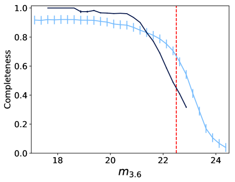
Figure 2: Mean detection (light blue) and membership (dark blue) completeness for the clusters in our sample. The error bars on the detection completeness are Poisson errors and the error bars on the membership completeness are from bootstrap resampling. At the bright end of the membership completeness curve ($3.6~{}\mathrm{\mu m}$$<18.75$) there were not enough field objects to produce meaningful statistics, so we fixed the completeness to unity. The vertical dashed red line at the faint end represents the average $5\sigma$ detection limit.

3.3 Stellar Mass

We used another SED-fitting program, FAST (Kriek et al., 2009), on the cluster catalogs to calculate the stellar masses of the objects along the line of sight to the cluster. For this, we adopted a Bruzual & Charlot (2003) model, a Chabrier (2003) initial mass function, a solar metallicity, and we fixed the redshift of each object in the catalog to the cluster redshift. We only fit to intrinsic properties of the galaxies, in particular stellar mass. As with the redshift fitting, we also ran FAST on the field catalog to calibrate the errors in our fitting and to establish how much field contribution to expect even after removing interlopers. Comparing the stellar masses we measured in this way to the stellar masses given in the COSMOS catalog, we adopted a uniform $0.2~{}\mathrm{dex}$ uncertainty in our stellar mass measurements.

With this final catalog of objects identified as being at the cluster redshift by EAZY, lying within a projected distance of $r_{500}$ from the cluster center, and with stellar masses measured from FAST, we calculated the total stellar mass of the clusters inside $r_{500}$. For each cluster, we first scaled the stellar mass of each object by the photometric and membership completeness corrections in §3.2. We then summed these scaled masses to get a total line-of-sight stellar mass for the cluster. Since this is still expected to include some small number of interlopers, we measured the total stellar mass of the statistical interloper catalog in the same way. We scaled that mass to the area of the cluster catalog and subtracted this expected interloper contribution—approximately 10% of the line-of-sight mass for most of the clusters—from the line-of-sight mass to get the total cluster stellar mass. We calculated the error on the stellar mass of each cluster by propagating the error of the stellar mass of each individual object in the cluster and field catalogs, measured in §3.1.

3.4 Luminosity Function

We used our membership selection and deep IRAC photometry to produce composite $3.6~{}\mathrm{\mu m}$ LFs for our cluster sample. For each cluster, we first evolution-corrected the $3.6~{}\mathrm{\mu m}$ apparent magnitudes of both the cluster and interloper catalog to the mean redshift of the sample using EZGal (Mancone & Gonzalez, 2012) and assuming passive evolution after an initial starburst at $z_{f}=3.0$. We removed the brightest cluster galaxy (BCG) from the cluster catalog and then binned these evolution-corrected catalogs into quarter-magnitude bins to produce a line-of-sight LF and a background LF for each cluster. We then applied both the completeness corrections described in §3.2 as a function of magnitude to both LFs. Finally, we scaled the background LF to match the surface area of the cluster and subtracted it off the line-of-sight LF to produce the individual cluster LF. These individual LFs were stacked to form the composite LF for the sample. The error on each value in the individual LFs is from adding in quadrature the Poisson errors of both the line-of-sight and interloper LFs and the errors on both completeness corrections. The error on each value in the composite LF is the quadrature sum of those errors from the individual LFs.

4 Results

4.1 Stellar Mass Fractions

The stellar mass fractions we measure for these clusters are given in Table 2 and Figure 3 shows $f_{\star}$ versus $M_{500}$ for the 12 clusters of this work, plotted as red diamonds. For comparison, we also plot the low-redshift trend line measured by Gonzalez et al. (2013) as a green dashed line. Clusters that were also studied in Decker et al. (2019) are indicated in Table 2.

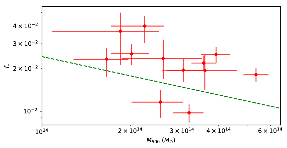
Figure 3: Stellar mass fraction versus total mass for the MaDCoWS clusters in this analysis, plotted as red diamonds. The error on $f_{\star}$ is from adding the percent stellar mass error from §3.3 and the percent error of the total mass of the cluster in quadrature. The green dashed line is the low-redshift relation from Gonzalez et al. (2013), plotted to provide continuity with Decker et al. (2019).

Table 2: MaDCoWS Stellar Mass Fractions

ID	$M_{500}$	$M_{\star}$	$f_{\star}$
	$(10^{14}~{}M_{\odot})$	$(10^{12}~{}M_{\odot})$	$(10^{-2})$
MOO J0105$+$1323*	$3.92^{+0.46}_{-0.44}$	$10.6\pm 0.58$	$2.70^{+0.35}_{-0.34}$
MOO J0319$-$0025*	$3.03^{+0.54}_{-0.46}$	$6.32\pm 0.49$	$2.09^{+0.40}_{-0.36}$
MOO J0917$-$0700	$1.66^{+0.31}_{-0.38}$	$4.08\pm 0.36$	$2.48^{+0.51}_{-0.61}$
MOO J1111$+$1503*	$2.02^{+0.30}_{-0.30}$	$4.95\pm 0.40$	$2.45^{+0.42}_{-0.42}$
MOO J1139$-$1706	$2.24^{+0.36}_{-0.52}$	$8.40\pm 0.66$	$3.80^{+0.68}_{-0.93}$
MOO J1142$+$1527*	$5.36^{+0.55}_{-0.50}$	$9.91\pm 0.59$	$1.85^{+0.22}_{-0.20}$
MOO J1155$+$3901*	$2.53^{+0.50}_{-0.51}$	$3.21\pm 0.29$	$1.27^{+0.28}_{-0.28}$
MOO J1329$+$5647	$3.56^{+0.35}_{-0.33}$	$7.89\pm 0.64$	$2.25^{+0.28}_{-0.27}$
MOO J1506$+$5136	$3.17^{+0.38}_{-0.37}$	$3.59\pm 0.27$	$1.16^{+0.16}_{-0.16}$
MOO J1514$+$1346*	$2.39^{+0.51}_{-0.83}$	$7.34\pm 0.49$	$3.97^{+1.42}_{-1.67}$
MOO J1521$+$0452*	$3.59^{+1.02}_{-0.92}$	$7.15\pm 0.60$	$1.99^{+0.59}_{-0.54}$
MOO J2206$+$0906*	$2.95^{+0.82}_{-0.68}$	$6.52\pm 0.40$	$2.52^{+0.90}_{-0.72}$

Figure 4 shows the direct comparison of $f_{\star}$ for the eight clusters common to both this work and Decker et al. (2019). With only one exception, MOO J0105$+$1323, the $f_{\star}$ we measure in this work is higher than the $f_{\star}$ we found in Decker et al. (2019) and for no clusters is it significantly lower. This is expected as in both works we use IRAC $3.6~{}\mathrm{\mu m}$ to measure $f_{\star}$—either directly or indirectly—and the much deeper $3.6~{}\mathrm{\mu m}$ data in this work allow us to include stellar mass from galaxies that were too faint to be Using $3.6~{}\mathrm{\mu m}$ luminosity as a proxy for stellar mass, we quantify the amount of ‘extra’ stellar mass we should expect with these deeper data by integrating down the composite LF we measure in §4.2. Integrating down to the depth of our current data versus integrating to the depth of our data in Decker et al. (2019) shows we are sensitive to approximately 25% more stellar mass with these deep IRAC data than we were previously. This is consistent with the change in $f_{\star}$ we see in all but two of the clusters. Further integrating the LF arbitrarily deep shows this analysis is sensitive to $\geq 95\%$ of the stellar mass in each cluster.

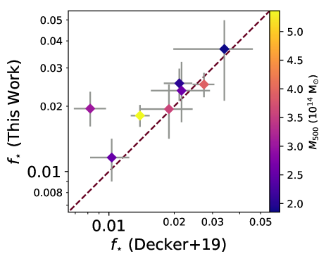
Figure 4: Comparison of the stellar mass fractions of clusters common to this work and to Decker et al. (2019). The dashed red line represents where the old and new mass fractions would be equal. Clusters falling above the line have a higher $f_{\star}$ in this work and clusters falling below the line have a higher $f_{\star}$ in Decker et al. (2019). The color of each point corresponds to the mass of the cluster.

MOO J0319$-$0025 and MOO J1142$+$1527 exhibit larger jumps in $f_{\star}$ than the 25% we expect simply from the deeper data. Those increases likely come from the improved way we are determining both cluster membership and stellar mass. Using a fuller sampling of the galaxy SEDs—even in just four bands—gives us a better and more consistent measurement of the stellar mass of each object versus what we were able to do in Decker et al. (2019).

4.2 Luminosity Functions

Table 3: MaDCoWS Sample Data and Schechter Parameters

Sample	Ncl	$\bar{z}$	$\bar{M_{500}}$	$m^{*}$	$\alpha$	$\phi^{*}$
			($10^{14}M_{\odot}$)			($\mathrm{dN}~{}\mathrm{dm}^{-1}~{}\mathrm{cluster}^{-1}$)
All	12	1.18	$2.96$	$19.83\pm 0.12$	$-0.81\pm 0.10$	$98\pm 13$
High-$z$	6	1.29	$3.30$	$19.86\pm 0.20$	$-0.95\pm 0.15$	$89\pm 20$
Low-$z$	6	1.06	$2.62$	$19.69\pm 0.22$	$-0.77\pm 0.16$	$96\pm 20$

The composite LF for our full sample of 12 clusters is shown in Figure 5. We fit a parameterized Schechter function to the measured LF using a Monte Carlo Markov Chain (MCMC) running a Metropolis-Hastings algorithm. The best-fit Schechter function is shown as a dashed line in the figure, with the lighter region showing the $1\sigma$ error on the best fit. The best fit parameters and the error on them are derived from the mean and standard deviation of the MCMC posterior chains after discarding the initial ‘burn-in’ period. These values are listed in Table 3 along with the mean redshift and mass of the sample.

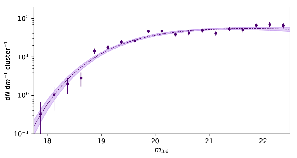
Figure 5: Composite LF for the full sample of 12 clusters used in this analysis. The purple points are the average number of objects per magnitude per cluster in each quarter-magnitude bin and the error bars are derived from the Poisson error of the individual LFs and the completeness errors. The mean sample mass and redshift are given, as well as the best fits to the parameterized Schechter function and their errors, in Table 3. The best-fit Schechter function itself is shown as a dashed line and the shaded area represents the $1\sigma$ error on the best fit.

Because $m^{*}$ and $\alpha$ are covariant, in addition to the simple errors given in Table 3, we also plot the $1\sigma$ (dark) and $2\sigma$ (light) covariance ellipses for $m^{*}$ and $\alpha$ for the full sample in Figure 6. This shows the extent of the degeneracy between $m^{*}$ and $\alpha$ as well as the axis along which our uncertainty is concentrated.

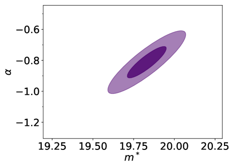
Figure 6: Covariance ellipses showing the $1\sigma$ (dark) and $2\sigma$ (light) errors and covariances in $m^{*}$ and $\alpha$ for the average LF of all 12 clusters in this work.

Our sample is large enough that we also split our clusters into high- and low-redshift samples—splitting them at the median redshift of our sample, $z=1.17$—and measure composite LFs for both of those. The measurement and fitting for these sub-samples is the same as for the full sample and the mean masses and redshifts for both sub-samples are also shown in Table 3, along with the best-fit Schechter function parameters to each LF. These LFs are shown in Figure 7. As with the full sample, we also plot the covariance between $m^{*}$ and $\alpha$ for these two sub-samples in Figure 8. This figure shows that although the error bars for the individual parameters overlap between the two samples, there is a significant evolution from $z=1.29$ to $z=1.06$ in the LF as a whole. As discussed in §5.2.3, this is consistent with being driven by passive evolution in our sample. For comparison, we also plot in Figure 8 the outlines of the ellipses for the full sample from Figure 6.

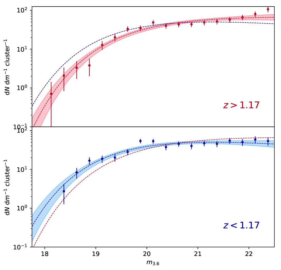
Figure 7: LFs for the high-redshift (upper, red) and low-redshift (lower, blue) subsamples. The best-fit Schechter functions are plotted as dashed lines with the $1\sigma$ error on the best fit shown as shaded regions. Each panel also shows the best fit line from the other panel as a dashed line of the relevant color.

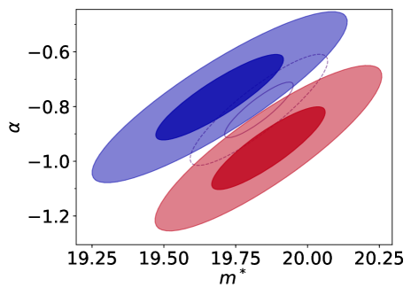
Figure 8: Covariance ellipses showing the $1\sigma$ (dark) and $2\sigma$ (light) errors and covariances in $m^{*}$ and $\alpha$ for the high-redshift (red) and low-redshift (blue) sub-samples. For comparison, the whole-sample covariances ellipses from Figure 6 are outlined underneath.

We also explore fitting a sum of two Schechter function to our LFs, in a manner similar to Lan et al. (2016). This is motivated particularly by our high-redshift LF which seems to show an upturn at the faint end that is possibly more consistent with a second ‘faint’ Schechter function wit a steep faint-end slope. Although we can’t rule out there being an upturn at the faint-end of our LFs, to the depth of our data ($\sim m^{*}+2.5$) we find that this sum of Schechter functions is at best only a marginally better fit to the data, at a level that is well short of statistical significance.

5 Discussion

5.1 Stellar Mass Fraction

The stellar mass fractions we compute in this work display many of the same traits as the stellar mass fractions we calculated in Decker et al. (2019). The main difference is that the improved measurement of $f_{\star}$ has resulted in higher values overall, and ten of the twelve now lie slightly above the Gonzalez et al. (2013) line, nine of them significantly so. They still appear to follow the slope of the Gonzalez et al. (2013) line, however. Despite our improved measurements significantly reducing the systematic errors on our measurements of $f_{\star}$, the statistical errors are still high enough that we cannot draw any significant conclusions about either the slope of the trend or its normalization. Much of this is due to the high error on the total mass of some of the clusters, which factors into the error on $f_{\star}$. For the well-measured clusters like MOO J1142$+$1527 on the right side of Figure 3, the $f_{\star}$ error is very small. Deeper SZ imaging on the MaDCoWS clusters is likely necessary to provide a significant measurement of properties related to the total mass.

5.2 Comparison to Other LF Studies

A comparison of our measurements of $m^{*}$ and $\alpha$ to other works across a range of redshifts is shown in Figures 9 and 10. To facilitate comparison with some other studies, we again use EZGal to convert our apparent $3.6~{}\mathrm{\mu m}$ magnitudes to absolute $H$-band magnitudes. We use a Bruzual & Charlot (2003) model with a formation redshift of $z_{f}=3.0$, a Chabrier (2003) initial mass function, and a solar metallicity to calculate the $k$-correction, but because we are already probing the rest-frame $H$-band with our $3.6~{}\mathrm{\mu m}$ observations, the $k$-correction is almost entirely model-independent and changing the model parameters does not affect the $k$-correction by more than $0.01$ at any of our redshifts. Doing this, we find $M_{H}^{*}=-23.91\pm 0.12$ for our overall LF and $M_{H}^{*}=-24.09\pm 0.20$ and $M_{H}^{*}=-23.80\pm 0.22$ for the high- and low-redshift LFs, respectively. Figure 9 shows this comparison for $M_{H}^{*}$.

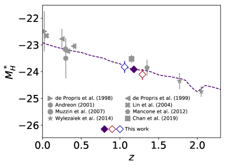
Figure 9: Absolute $H$-band characteristic magnitude versus redshift for a number of cluster LF studies. The error on the Lin et al. (2004) point is 0.02, smaller than the data marker. The dashed purple line shows the expected passive evolution in $M^{*}_{H}$

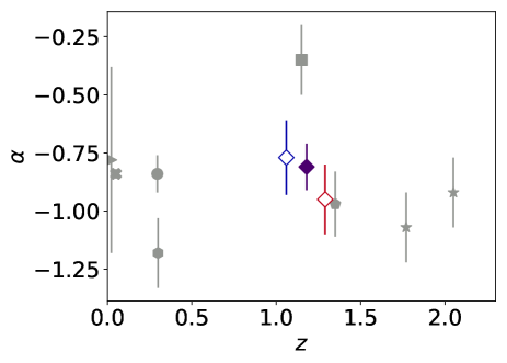
Figure 10: Faint-end slope versus redshift for a number of cluster LF studies. The labels for the points are the same as in Figure 9. The error on the Lin et al. (2004) point is 0.02, smaller than the data marker.

For both $M^{*}$ and $\alpha$ we plot the results from our full sample as a solid diamond and the results from the high- and low-redshift samples as red and blue open diamonds, respectively. In Figure 9, we also plot as a dashed line the expected trend of $M^{*}_{H}$ with redshift, assuming passive evolution. We discuss the comparison works below.

5.2.1 Comparisons at Similar Redshift

Owing to the difficulty in getting deep enough mid-infrared data, few studies have previously been able to measure both $m^{*}$ and $\alpha$ simultaneously at this redshift range. One such study is Mancone et al. (2012), who measured composite LFs in $3.6~{}\mathrm{\mu m}$ and $4.5~{}\mathrm{\mu m}$ for seven IRAC Shallow Cluster Survey (ISCS) clusters at a median redshift of $z=1.35$, slightly higher than our mean redshift overall, but a good match to our high-redshift sub-sample. Converting the apparent Vega magnitudes they report into absolute AB magnitudes, they found best fit parameters for the $3.6~{}\mathrm{\mu m}$ LF of $M_{H}^{*}=-23.85\pm 0.30$ and $\alpha=-0.97\pm 0.14$. The faint-end slope we measure for the high-redshift clusters matches this result almost exactly and the characteristic magnitude we find is also consistent with their results.

Another similar study is Chan et al. (2019), who used IRAC $3.6~{}\mathrm{\mu m}$ imaging to measure rest-frame $H$-band LFs for red-sequence galaxies in seven clusters from the infrared-selected Gemini Observations of Galaxies in Rich Early Environments (GOGREEN, Balogh et al., 2017) survey at a mean redshift of $\bar{z}=1.15$. They report their results in terms of absolute $H$-band magnitudes and find $M_{H}^{*}=-23.52^{+0.15}_{-0.17}$, which is somewhat fainter than our value of $M_{H}^{*}=-23.91\pm 0.12$ at $z=1.18$. They also find a much more steeply falling faint-end slope than we do, with a value of $\alpha=-0.35\pm 0.15$. This difference in $\alpha$ may be a result of their only including red-sequence galaxies, whereas we include everything with a photometric redshift consistent with being a cluster member. Other works (e.g., Muzzin et al., 2007; Strazzullo et al., 2006; De Propris, 2017) have found that the faint-end of the cluster LF is dominated by blue galaxies, which would explain the discrepancy between our results and red-sequence-only results. Alternatively, Connor et al. (2019) found that the traditional model of the red sequence as a sloped line does not hold at fainter magnitudes. This could cause a drop-off in the measured red-sequence LF that is unconnected to the galaxy population of the cluster.

5.2.2 Comparisons at Other Redshifts

To put our results into a wider context, we also compare to studies at other redshifts and with different cluster selection and fitting methods. To make as fair a comparison as possible to $m^{*}$ at other redshifts, we use the model described in §5.2 to convert all the magnitudes into the absolute $H$-band and limit ourselves to studies where the reported values still probe either the rest-frame $H$-band or nearby $K$-band. These comparisons are also shown in Figures 9 and 10.

At the lowest-redshift of our comparisons, de Propris et al. (1998) looked at the Coma cluster at $z=0.023$ to a depth much fainter than $m^{*}$. They jointly fit $m^{*}$ and $\alpha$ at magnitudes brighter than $m^{*}+3$, though at magnitudes fainter than $m^{*}+3$, they found a sharp rise in the number of galaxies and fit this with a power law. At a similar redshift, Lin et al. (2004) calculated a stacked $K$-band LF for a sample of 13 Abell clusters with X-ray follow-up. We compare to their joint fits of $m^{*}$ and $\alpha$, though they also attempt to fix $\alpha$ due to the uncertainty in the faint-end slope. Their errors on both parameters are $0.02$, which is small enough it does not appear on Figures 9 and 10. At higher redshift, de Propris et al. (1999) looked at a heterogenous selection of clusters in the $K$-band in redshift bins up to $z=0.92$. They only fit to $m^{*}$, fixing the faint-end slope at $\alpha=-0.9$. We compare $z=0.25$, $z=0.32$ and $z=0.4$ bins, where the conversion from $K$-band into rest-frame $H$-band has a minimal $k$-correction. Similarly, Muzzin et al. (2007), measured the observed-frame $K$-band for clusters at a mean redshift of $\bar{z}=0.296$. In addition to reporting a composite LF for all galaxies in their clusters, Muzzin et al. (2007) also split their galaxies by whether they were quiescent or star-forming/recently-quenched. They found a relatively flat faint-end slope for their overall LF, $\alpha=-0.84\pm 0.08$ and a much steeper faint-end slope of $\alpha=0.17\pm 0.18$ for red-sequence galaxies. At similar redshift, Andreon (2001) studied a single cluster at $z=0.3$ in the $K_{S}$-band. He measured a LF down to $m^{*}+5$ in various areas of the cluster, but the comparison we show is to the global values he reported. At higher redshifts, we also compare to some of the results from Wylezalek et al. (2014), who measured the $4.5~{}\mathrm{\mu m}$ and $3.6~{}\mathrm{\mu m}$ LF for clusters from the Clusters Around Radio Loud AGN program (CARLA, Wylezalek et al., 2013) in several redshift bins in the range $1.3<z<3.1$. We show two of these in Figures 9 and 10, again where the conversion from $3.6~{}\mathrm{\mu m}$ or $4.5~{}\mathrm{\mu m}$ has a minimal $k$-correction.

5.2.3 Evolution of the LF

Figure 9 shows the clusters in this work fall into a larger pattern of passive evolution in $M_{H}^{*}$ going out to $z\sim 2$. Similarly, Figure 10 shows very little change in the faint-end slope over cosmic time when looking only at $\alpha$ over a range of studies. This suggests that the evolution in the parameters shown in Figure 8 is primarily driven by passive evolution.

To confirm this, we evolution-correct the galaxies in the high- and low-redshift sub-samples to $z=1.18$, the mean redshift of the full sample, assuming passive evolution. We then re-make the LFs and run the same joint fit as above. The results of this are shown in Figure 11. With passive-evolution ‘baked-in’ to the fit, the LF parameters are now consistent within two sigma, supporting the interpretation that these clusters are evolving passively, consistent with other studies at this redshift.

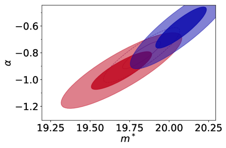
Figure 11: Covariance ellipses showing the $1\sigma$ (dark) and $2\sigma$ (light) errors and covariances in $m^{*}$ and $\alpha$ for the high-redshift (red) and low-redshift (blue) sub-samples, assuming passive evolution. For comparison, the whole-sample covariances ellipses from Figure 6 are outlined underneath.

6 Conclusions

We have presented stellar mass fractions and $3.6~{}\mathrm{\mu m}$ LFs for a sample of 12 infrared-selected clusters from the MaDCoWS catalog. We used optical and deep mid-IR follow-up data to fit SEDs to objects along the lines-of-sight to the clusters. This allowed us to more precisely identify cluster members, measure more thorough stellar masses for the clusters and measure the faint-end slope of the LF.

The stellar mass fractions we report for these clusters are in good agreement with previous works, and are consistent with the Gonzalez et al. (2013) trend line with respect to total mass. For the individual clusters previously studied in Decker et al. (2019), the new values of $f_{\star}$ reported here are consistent with—but mostly higher than—the previous values, with much of the difference being attributable to the deeper data set we use here.

The composite $3.6~{}\mathrm{\mu m}$ LF we fit for all 12 clusters has a best-fit characteristic magnitude and faint-end slope of $m^{*}=19.83\pm 0.12$ and $\alpha=-0.81\pm 0.10$, respectively. Both are consistent with other works that have attempted to measure the rest-frame NIR LF for all cluster members at these redshift ranges. When we split our sample into a high-redshift bin at $\bar{z}=1.29$ and a low-redshift bin at $\bar{z}=1.06$ we find that there is a significant evolution in the best-fit Schechter function parameters, consistent with passive evolution. This significance is only seen in the covariance ellipse for $m^{*}$ and $\alpha$ jointly. This highlights the need to study $m^{*}$ and $\alpha$ jointly. Comparing to works at other redshifts, our results are consistent with passive evolution since $z\sim 2$.

In future, follow-up data on more MaDCoWS clusters will allow us to better identify trends with redshift and other cluster parameters. In addition, deeper infrared data—such as will be attainable from the next generation of IR space telescopes—will allow us to more definitively answer questions about the evolution of the faint galaxy population in clusters at $z>1$.

References

- Andreon (2001) Andreon, S. 2001, ApJ, 547, 623
- Ashby et al. (2009) Ashby, M. L. N., Stern, D., Brodwin, M., et al. 2009, ApJ, 701, 428
- Ashby et al. (2013) Ashby, M. L. N., Willner, S. P., Fazio, G. G., et al. 2013, ApJ, 769, 80
- Balogh et al. (2017) Balogh, M. L., Gilbank, D. G., Muzzin, A., et al. 2017, MNRAS, 470, 4168
- Bertin & Arnouts (1996) Bertin, E. & Arnouts, S. 1996, A&AS, 117, 393
- Bertin et al. (2002) Bertin, E., Mellier, Y., Radovich, M., et al. 2002, in Astronomical Society of the Pacific Conference Series, Vol. 281, Astronomical Data Analysis Software and Systems XI, ed. D. A. Bohlender, D. Durand, & T. H. Handley, 228
- Brammer et al. (2008) Brammer, G. B., van Dokkum, P. G., & Coppi, P. 2008, ApJ, 686, 1503
- Brodwin et al. (2015) Brodwin, M., Greer, C. H., Leitch, E. M., et al. 2015, ApJ, 806, 26
- Bruzual & Charlot (2003) Bruzual, G. & Charlot, S. 2003, MNRAS, 344, 1000
- Chabrier (2003) Chabrier, G. 2003, PASP, 115, 763
- Chan et al. (2019) Chan, J. C. C., Wilson, G., Rudnick, G., et al. 2019, ApJ, 880, 119
- Connor et al. (2019) Connor, T., Kelson, D. D., Donahue, M., & Moustakas, J. 2019, ApJ, 875, 16
- Conroy et al. (2007) Conroy, C., Wechsler, R. H., & Kravtsov, A. V. 2007, ApJ, 668, 826
- De Propris (2017) De Propris, R. 2017, MNRAS, 465, 4035
- de Propris et al. (1998) de Propris, R., Eisenhardt, P. R., Stanford, S. A., & Dickinson, M. 1998, ApJ, 503, L45
- de Propris et al. (1999) de Propris, R., Stanford, S. A., Eisenhardt, P. R., Dickinson, M., & Elston, R. 1999, AJ, 118, 719
- Decker et al. (2019) Decker, B., Brodwin, M., Abdulla, Z., et al. 2019, ApJ, 878, 72
- Di Mascolo et al. (2020) Di Mascolo, L., Mroczkowski, T., Churazov, E., et al. 2020, A&A, 638, A70
- Dicker et al. (2020) Dicker, S. R., Romero, C. E., Di Mascolo, L., et al. 2020, ApJ, 902, 144
- Ettori et al. (2006) Ettori, S., Dolag, K., Borgani, S., & Murante, G. 2006, MNRAS, 365, 1021
- Fazio et al. (2004) Fazio, G. G., Hora, J. L., Allen, L. E., et al. 2004, ApJS, 154, 10
- Gonzalez et al. (2013) Gonzalez, A. H., Sivanandam, S., Zabludoff, A. I., & Zaritsky, D. 2013, ApJ, 778, 14
- Gonzalez et al. (2015) Gonzalez, A. H., Decker, B., Brodwin, M., et al. 2015, ApJ, 812, L40
- Gonzalez et al. (2019) Gonzalez, A. H., Gettings, D. P., Brodwin, M., et al. 2019, ApJS, 240, 33
- Hook et al. (2004) Hook, I. M., Jørgensen, I., Allington-Smith, J. R., et al. 2004, PASP, 116, 425
- Kauffmann & Charlot (1998) Kauffmann, G. & Charlot, S. 1998, MNRAS, 297, L23
- Kriek et al. (2009) Kriek, M., van Dokkum, P. G., Labbé, I., et al. 2009, ApJ, 700, 221
- Laigle et al. (2016) Laigle, C., McCracken, H. J., Ilbert, O., et al. 2016, ApJS, 224, 24
- Lan et al. (2016) Lan, T.-W., Ménard, B., & Mo, H. 2016, MNRAS, 459, 3998
- Lin et al. (2003) Lin, Y.-T., Mohr, J. J., & Stanford, S. A. 2003, ApJ, 591, 749
- Lin et al. (2004) Lin, Y.-T., Mohr, J. J., & Stanford, S. A. 2004, ApJ, 610, 745
- Mancone & Gonzalez (2012) Mancone, C. L. & Gonzalez, A. H. 2012, PASP, 124, 606
- Mancone et al. (2012) Mancone, C. L., Gonzalez, A. H., Brodwin, M., et al. 2012, ApJ, 761, 141
- Muzzin et al. (2007) Muzzin, A., Yee, H. K. C., Hall, P. B., Ellingson, E., & Lin, H. 2007, ApJ, 659, 1106
- Orlowski-Scherer et al. (2021) Orlowski-Scherer, J., Di Mascolo, L., Bhandarkar, T., et al. 2021, A&A, 653, A135
- Schechter (1976) Schechter, P. 1976, ApJ, 203, 297
- Scoville et al. (2007) Scoville, N., Aussel, H., Brusa, M., et al. 2007, ApJS, 172, 1
- Strazzullo et al. (2006) Strazzullo, V., Rosati, P., Stanford, S. A., et al. 2006, A&A, 450, 909
- Sunyaev & Zeldovich (1970) Sunyaev, R. A. & Zeldovich, Y. B. 1970, Comments on Astrophysics and Space Physics, 2, 66
- Sunyaev & Zeldovich (1972) Sunyaev, R. A. & Zeldovich, Y. B. 1972, Comments on Astrophysics and Space Physics, 4, 173
- Wylezalek et al. (2013) Wylezalek, D., Galametz, A., Stern, D., et al. 2013, ApJ, 769, 79
- Wylezalek et al. (2014) Wylezalek, D., Vernet, J., De Breuck, C., et al. 2014, ApJ, 786, 17