The truncated $\theta$-Milstein method for nonautonomous and highly nonlinear stochastic differential delay equations

Abstract

This paper focuses on the strong convergence of the truncated $\theta$-Milstein method for a class of nonautonomous stochastic differential delay equations whose drift and diffusion coefficients can grow polynomially. The convergence rate, which is close to one, is given under the weaker assumption than the monotone condition. To verify our theoretical findings, we present a numerical example.

1 Introduction

The research on stochastic differential equations (SDEs) has been widely concerned due to their applications in numerous fields such as finance, communication, biology, chemistry, and ecology [1, 4, 27, 31]. It is well known that time delay is widespread in nature and occurs in dynamics with a finite propagation time, then the corresponding stochastic differential delay equations (SDDEs) are widely applied in stochastic systems [6, 24, 26, 28, 35, 36, 37, 44]. In plenty of instances, the true solutions to SDEs cannot be expressed explicitly. Hence, it is very meaningful to simulate the true solutions with different numerical algorithms; in this way, scholars can grasp a lot of significant properties of the true solutions without knowing the explicit form of the true solutions. One of the most famous numerical methods for a SDE is Euler-Maruyama (EM) method, which has been investigated and developed in the past few decades [20, 27, 31]. Unfortunately, Hutzenthaler et al. have proved that the $p$th($p\geq 1$) moment of the EM solutions would diverge to infinity if the coefficients grow super-linearly in [18]. To approximate the stochastic equations with highly nonlinear growing coefficients, many implicit methods have been studied [3, 14, 32, 33, 37, 43]. Furthermore, some modified explict schemes have been established as well, since they have less computational cost [5, 19, 34, 38]. Particularly, it is worth emphasizing that the truncated EM method for SDEs was initially established by Mao in [29] and the convergence rate was obtained in [30]. Since then, some scholars have studied SDEs whose coefficients can grow super-linearly by using the truncated EM method, and we can refer to [8, 9, 10, 11, 13, 22, 25] and references therein. To improve the convergence rate, Guo et al. [12] established the truncated Milstein method (TMM) to approximate SDEs with commutative noise. Thereafter, the TMM for nonautonomous SDEs was analyzed in [23]. The convergence rate of the TMM for SDDEs was investigated in [42]. As for other papers about Milstein methods, we refer the readers to [7, 16, 17, 21, 33, 38, 39, 45] for more detailed discussions.

The aim of this paper is to study the strong convergence rate of the truncated $\theta$-Milstein method for nonautonomous and highly nonlinear SDDEs. The main contributions of this paper are as follows.

• The SDDEs in this paper are nonautonomous, unlike many studies that focus on autonomous case. It is worth noting that the autonomy of the equation will affect the convergence rate of the numerical scheme.

• The truncated $\theta$-Milstein method for nonautonomous SDDEs is established in this paper, and it will degenerate into the TMM when $\theta=0$.

• The convergence rate in $\mathcal{L}^{2}$ sense can be obtained with the more relaxed assumptions than those in [42], which is given in Remark 1.

• We relax the requirements for establishing the numerical scheme, which is shown in Remark 2.

• The convergence rate in $\mathcal{L}^{\bar{q}}(\bar{q}\geq 2)$ sense is presented in this paper, but [42] only gives the convergence rate in $\mathcal{L}^{2}$ sense, which can be found in Theorems 3.15 and 3.19.

This paper is organized as follows. Some necessary notations and the structure of the truncated $\theta$-Milstein method are shown in Section 2. Main result are presented in Section 3. Section 4 contains an example. The conclusion and discussion on future research are stated in Section 5.

2 Preliminaries

We use the following notations throughout this paper. Let $|x|$ denote its Euclidean norm for $x\in\mathbb{R}^{n}$. Define $a\wedge b=\text{min}\{a,b\}$ and $a\vee b=\text{max}\{a,b\}$ for any real numbers $a,b$. Let $\left\lfloor a\right\rfloor$ be the largest integer which is not greater than $a$. Let the delay constant $\tau>0$. Then let $\mathcal{C}([-\tau,0];\mathbb{R})$ be the family of all continuous functions $\xi$ from $[-\tau,0]$ to $\mathbb{R}$ with the norm $\|\xi\|=\text{sup}_{-\tau\leq\theta\leq 0}|\xi(\theta)|$. If $S$ is a set, let $\mathbb{I}_{S}$ be its indicator function, which means that $\mathbb{I}_{S}(x)=1$ if $x\in S$ and $\mathbb{I}_{S}(x)=0$ if $x\notin S$. Set $\mathbb{R}_{+}=[0,+\infty)$. Suppose that $C$ is a positive real constant which may be different in different cases.

Let $\big{(}\Omega,\mathcal{F},\{\mathcal{F}_{t}\}_{t\geq 0},\mathbb{P}\big{)}$ stand for a complete probability space with a filtration $\{\mathcal{F}_{t}\}_{t\geq 0}$ which satisfies the usual conditions (i.e., it is increasing and right continuous while $\mathcal{F}_{0}$ contains all $\mathbb{P}$-null sets). Denote by $\mathbb{E}$ the probability expectation. Let $\mathcal{L}^{p}=\mathcal{L}^{p}(\Omega,\mathcal{F},\mathbb{P}\big{)}$ for $p>0$ be the space of all random variables $X$ with $\mathbb{E}|X|^{p}<\infty$. Let $\mathcal{C}_{\mathcal{F}_{0}}^{b}([-\tau,0];\mathbb{R})$ stand for the family of $\mathcal{F}_{0}$-measurable, $\mathcal{C}([-\tau,0];\mathbb{R})$-valued, bounded random variables. Let $B(t)$ stand for a $1$-dimensional Brownian motion.

Consider the 1-dimensional nonautonomous and highly nonlinear SDDEs of the form

$$dx(t)=f\left(t,x(t),x(t-\tau)\right)dt+g\left(t,x(t),x(t-\tau)\right)dB(t),$$ (2.1)

on $t\geq 0$ with the initial data

$$x_{0}=\xi=\{\xi(\theta):-\tau\leq\theta\leq 0\}\in\mathcal{C}^{b}_{\mathcal{F}_{0}}([-\tau,0];\mathbb{R}),$$ (2.2)

where $f:\mathbb{R_{+}}\times\mathbb{R}\times\mathbb{R}\rightarrow\mathbb{R}$ and $g:\mathbb{R_{+}}\times\mathbb{R}\times\mathbb{R}\rightarrow\mathbb{R}$.

In order to study the strong convergence rate of the truncated $\theta$-Milstein method for nonautonomous and highly nonlinear SDDEs (2.1), the following assumptions need to be imposed.

Assumption 2.1.

There exist constants $\bar{K}>0$ and $\beta\geq 0$ such that

$$\begin{split}&|f(t,a,b)-f(t,\bar{a},\bar{b})|\vee|g(t,a,b)-g(t,\bar{a},\bar{b})|\\ &\leq\bar{K}(1+|a|^{\beta}+|b|^{\beta}+|\bar{a}|^{\beta}+|\bar{b}|^{\beta})(|a-\bar{a}|+|b-\bar{b}|)\end{split}$$

for any $t\in[0,T]$ and $a,b,\bar{a},\bar{b}\in\mathbb{R}$.

Before Assumption 2.2, we give more notations. Let $\bar{\mathcal{U}}$ be the family of all continuous functions $U:\mathbb{R}\times\mathbb{R}\rightarrow\mathbb{R}_{+}$ such that for $\varsigma>0$, there is a constant $\rho_{\varsigma}>0$, which satisfies

$$U(m,n)\leq\rho_{\varsigma}|m-n|^{2}$$ (2.3)

for any $m,n\in\mathbb{R}$ with $|m|\vee|n|\leq\varsigma$.

Assumption 2.2.

There exist constants $K_{1}>0$ and $q>2$ such that

$$\begin{split}&(a-\bar{a})^{T}(f(t,a,b)-f(t,\bar{a},\bar{b}))+(q-1)|g(t,a,b)-g(t,\bar{a},\bar{b})|^{2}\\ &\leq K_{1}(|a-\bar{a}|^{2}+|b-\bar{b}|^{2})-U(a,\bar{a})+U(b,\bar{b})\end{split}$$

for any $t\in[0,T]$ and $a,b,\bar{a},\bar{b}\in\mathbb{R}$.

Remark 1.

An example is given to show that Assumption 2.2 is weaker than (A3) in [42] by introducing $U(\cdot,\cdot)$. Let $f(a,b)=\frac{1}{8}|b|^{\frac{5}{4}}-5a^{3}+2\zeta_{t}a$, $g(a,b)=\frac{1}{2}|a|^{\frac{3}{2}}+\zeta_{t}b$, $\zeta_{t}=[t(1-t)]^{\frac{3}{4}}$ for $t\in[0,1]$ and $a,b\in\mathbb{R}$. One can see that there is no $K_{1}$ which satisfies

$$\begin{split}&(a-\bar{a})^{T}(f(t,a,b)-f(t,\bar{a},\bar{b}))+(q-1)|g(t,a,b)-g(t,\bar{a},\bar{b})|^{2}\\ &\leq K_{1}(|a-\bar{a}|^{2}+|b-\bar{b}|^{2}),\end{split}$$

however, Assumption 2.2 holds. The detailed proof can be found in Section 4.

Assumption 2.3.

There exist constants $K_{2}>0$ and $p>q$ such that

$$a^{T}f(t,a,b)+(p-1)|g(t,a,b)|^{2}\leq K_{2}(1+|a|^{2}+|b|^{2})$$

for any $t\in[0,T]$ and $a,b\in\mathbb{R}$.

Assumption 2.4.

There exist constants $K_{3}>0$ , $\beta\geq 0$ and $\sigma\in(0,1]$ such that

$$|f(t_{1},a,b)-f(t_{2},a,b)|\vee|g(t_{1},a,b)-g(t_{2},a,b)|\leq K_{3}(1+|a|^{\beta+1}+|b|^{\beta+1})|t_{1}-t_{2}|^{\sigma}$$

for any $t_{1},t_{2}\in[0,T]$ and $a,b\in\mathbb{R}$.

Assumption 2.5.

There exist constants $K_{4}>0$ and $\gamma\in(0,1]$ such that

$$|\xi(t)-\xi(s)|\leq K_{4}|t-s|^{\gamma}$$

for all $t,s\in[-\tau,0]$.

Assumption 2.6.

There exist constants $K_{5}>0$ and $\beta\geq 0$ such that

$$\begin{split}&|f_{i}(t,a,b)|\vee|g_{i}(t,a,b)|\vee|f_{ij}(t,a,b)|\vee|g_{ij}(t,a,b)|\leq K_{5}(1+|a|^{\beta+1}+|b|^{\beta+1}),\end{split}$$

where

$$\begin{split}&f_{i}(t,a_{1},a_{2})=\frac{\partial f(t,a_{1},a_{2})}{\partial a_{i}},~{}~{}~{}g_{i}(t,a_{1},a_{2})=\frac{\partial g(t,a_{1},a_{2})}{\partial a_{i}},\\ &f_{ij}(t,a_{1},a_{2})=\frac{\partial^{2}f(t,a_{1},a_{2})}{\partial a_{i}\partial a_{j}},~{}~{}~{}g_{ij}(t,a_{1},a_{2})=\frac{\partial^{2}g(t,a_{1},a_{2})}{\partial a_{i}\partial a_{j}},\\ \end{split}$$ (2.4)

for any $t\in[0,T],a,b,a_{1},a_{2}\in\mathbb{R}$ and $i,j=1,2$.

The notations in (2.4) will be used in the rest of this paper. The following lemma can be obtained with the standard method.

Lemma 2.7.

Let Assumptions 2.1-2.3 hold. There exists a unique global solution $x(t)$ to SDDE (2.1), which satisfies

$$\sup_{0\leq t\leq T}\mathbb{E}|x(t)|^{p}\leq C,~{}~{}~{}\forall T\geq 0.$$

In order to define the truncated $\theta$-Milstein method, choose a continuous and strictly increasing function $\Lambda:\mathbb{R}_{+}\rightarrow\mathbb{R}_{+}$ such that $\Lambda(w)\to\infty$ when $w\rightarrow\infty$, and

$$\sup_{0\leq t\leq T}\sup_{|x|\vee|y|\leq w}\left(|f(t,x,y)|\vee|g(t,x,y)|\vee|g_{1}(t,x,y)|\vee|g_{2}(t,x,y)|\right)\leq\Lambda(w),~{}~{}~{}\forall w\geq 1.$$ (2.5)

Denote by $\Lambda^{-1}$ the inverse function of $\Lambda$. Therefore, $\Lambda^{-1}$ is a strictly increasing continuous function from $[\Lambda(1),\infty)$ to $[1,\infty)$. Next, choose $K_{0}\geq[1\vee\Lambda(1)]$ and a strictly decreasing function $\alpha:(0,1]\rightarrow(0,\infty)$ such that

$$\lim_{\Delta\rightarrow 0}\alpha(\Delta)=\infty,~{}~{}~{}\Delta^{\frac{1}{4}}\alpha(\Delta)\leq K_{0},~{}~{}~{}\forall\Delta\in(0,1].$$ (2.6)

Remark 2.

The condition (2.6) is weaker than that in [42]. Here, let $K_{0}=1$, then $\Delta\in(0,\frac{1}{\alpha(\Delta)^{4}}]$. In [42], $\Delta\in(0,\frac{1}{\alpha(\Delta)^{6}}]$. Obviously, the step size $\Delta$ in our paper has a wider range than that in [42], which will lead to less computation, so we have more advantages in algorithm than [42]. As for other details, please refer to Remark 2.4 in [15].

The truncated mapping $\pi_{\Delta}:\mathbb{R}\rightarrow\mathbb{R}$ for the given step size $\Delta\in(0,1]$ is defined as

$$\pi_{\Delta}(\chi)=(|\chi|\wedge\Lambda^{-1}(\alpha(\Delta)))\frac{\chi}{|\chi|},$$ (2.7)

where let $\chi/|\chi|=0$ when $\chi=0$. One can see that $\pi_{\Delta}$ can map $\chi$ to itself when $|\chi|\leq\Lambda^{-1}(\alpha(\Delta))$, and to $\Lambda^{-1}(\alpha(\Delta))$ when $|\chi|>\Lambda^{-1}(\alpha(\Delta))$. Then define

$$f_{\Delta}(t,x,y)=f(t,\pi_{\Delta}(x),\pi_{\Delta}(y)),~{}~{}~{}g_{\Delta}(t,x,y)=g(t,\pi_{\Delta}(x),\pi_{\Delta}(y)),$$

$$g_{1,\Delta}(t,x,y)=g_{1}(t,\pi_{\Delta}(x),\pi_{\Delta}(y)),~{}~{}~{}g_{2,\Delta}(t,x,y)=g_{2}(t,\pi_{\Delta}(x),\pi_{\Delta}(y)).$$

By the definition, one has that

$$|f_{\Delta}(t,x,y)|\vee|g_{\Delta}(t,x,y)|\vee|g_{1,\Delta}(t,x,y)|\vee|g_{2,\Delta}(t,x,y)|\leq\alpha(\Delta).$$ (2.8)

Lemma 2.8.

By Assumption 2.3, for any $\Delta\in(0,1]$, we have

$$x^{T}f_{\Delta}(t,x,y)+(p-1)|g_{\Delta}(t,x,y)|^{2}\leq\bar{K}_{2}(1+|x|^{2}+|y|^{2})$$

for any $t\in[0,T]$ and $x,y\in\mathbb{R}$.

Lemma 2.8 can be proved with the technique in [41], so we omit the proof process.

Let us now define the truncated $\theta$-Milstein method to approximate the solution to (2.1). Suppose that $\Delta=\frac{\tau}{M}=\frac{T}{M^{\prime}}$ holds with integers $M$ and $M^{\prime}$. Without losing generality, set $M<M^{\prime}$. Let $t_{k}=k\Delta$ for $k=-M,\ldots,0,\ldots,M^{\prime}$. Then define

$$\left\{\begin{array}[]{l}Y_{\Delta}(t_{k})=\xi(t_{k}),~{}~{}~{}~{}~{}~{}~{}~{}~{}~{}~{}~{}~{}~{}~{}~{}~{}~{}~{}~{}~{}~{}~{}~{}~{}~{}~{}~{}~{}~{}~{}~{}~{}~{}~{}~{}~{}~{}~{}~{}~{}~{}k=-M,-M+1,\ldots,0;\\ Y_{\Delta}(t_{k+1})=Y_{\Delta}(t_{k})+\theta f_{\Delta}(t_{k+1},Y_{\Delta}(t_{k+1}),Y_{\Delta}(t_{k+1-M}))\Delta\\ ~{}~{}~{}~{}~{}~{}+(1-\theta)f_{\Delta}(t_{k},Y_{\Delta}(t_{k}),Y_{\Delta}(t_{k-M}))\Delta+g_{\Delta}(t_{k},Y_{\Delta}(t_{k}),Y_{\Delta}(t_{k-M}))\Delta B_{k}\\ ~{}~{}~{}~{}~{}~{}+g_{1,\Delta}(t_{k},Y_{\Delta}(t_{k}),Y_{\Delta}(t_{k-M}))g_{\Delta}(t_{k},Y_{\Delta}(t_{k}),Y_{\Delta}(t_{k-M}))Q_{1},\\ ~{}~{}~{}~{}~{}~{}~{}~{}~{}~{}~{}~{}~{}~{}~{}~{}~{}~{}~{}~{}~{}~{}~{}~{}~{}~{}~{}~{}~{}~{}~{}~{}~{}~{}~{}~{}~{}~{}~{}~{}~{}~{}~{}~{}~{}~{}~{}~{}~{}~{}~{}~{}~{}~{}~{}~{}~{}~{}~{}~{}~{}~{}~{}~{}~{}~{}~{}~{}~{}k=0,1,\ldots,M-1;\\ Y_{\Delta}(t_{k+1})=Y_{\Delta}(t_{k})+\theta f_{\Delta}(t_{k+1},Y_{\Delta}(t_{k+1}),Y_{\Delta}(t_{k+1-M}))\Delta\\ ~{}~{}~{}~{}~{}~{}+(1-\theta)f_{\Delta}(t_{k},Y_{\Delta}(t_{k}),Y_{\Delta}(t_{k-M}))\Delta+g_{\Delta}(t_{k},Y_{\Delta}(t_{k}),Y_{\Delta}(t_{k-M}))\Delta B_{k}\\ ~{}~{}~{}~{}~{}~{}+g_{1,\Delta}(t_{k},Y_{\Delta}(t_{k}),Y_{\Delta}(t_{k-M}))g_{\Delta}(t_{k},Y_{\Delta}(t_{k}),Y_{\Delta}(t_{k-M}))Q_{1}\\ ~{}~{}~{}~{}~{}~{}+g_{2,\Delta}(t_{k},Y_{\Delta}(t_{k}),Y_{\Delta}(t_{k-M}))g_{\Delta}(t_{k-M},Y_{\Delta}(t_{k-M}),Y_{\Delta}(t_{k-2M}))Q_{2},\\ ~{}~{}~{}~{}~{}~{}~{}~{}~{}~{}~{}~{}~{}~{}~{}~{}~{}~{}~{}~{}~{}~{}~{}~{}~{}~{}~{}~{}~{}~{}~{}~{}~{}~{}~{}~{}~{}~{}~{}~{}~{}~{}~{}~{}~{}~{}~{}~{}~{}~{}~{}~{}~{}~{}~{}~{}~{}~{}~{}~{}~{}k=M,M+1,\ldots,M^{\prime}-1.\end{array}\right.$$

where

$$\begin{split}Q_{1}=\int_{t_{k}}^{t_{k+1}}\int_{t_{k}}^{s}dB(t)dB(s)=\frac{(\Delta B_{k})^{2}-\Delta}{2},\end{split}$$

$$\begin{split}Q_{2}=\int_{t_{k}}^{t_{k+1}}\int_{t_{k}}^{s}dB(t-\tau)dB(s),~{}~{}~{}\Delta B_{k}=B(t_{k+1})-B(t_{k}).\end{split}$$

There is no doubt that we only need to analyze the case when $T>\tau$, which is equivalent to $M^{\prime}>M$. Define

$$\mu(t)=\sum_{k=0}^{M^{\prime}-1}t_{k}\mathbb{I}_{\left[t_{k},t_{k+1}\right)}(t),$$ (2.9)

and

$$\bar{\eta}_{\Delta}(t)=\sum_{k=-M}^{M^{\prime}-1}Y_{\Delta}\left(t_{k}\right)\mathbb{I}_{\left[t_{k},t_{k+1}\right)}(t).$$ (2.10)

The continuous form of the truncated $\theta$-Milstein method can be defined as

$$\begin{split}&\eta_{\Delta}(t)-\theta f_{\Delta}(t,\eta_{\Delta}(t),\eta_{\Delta}(t-\tau))\Delta\\ &=\xi(0)-\theta f_{\Delta}(0,\xi(0),\xi(-\tau))\Delta+\int_{0}^{t}f_{\Delta}(\mu(s),\bar{\eta}_{\Delta}(s),\bar{\eta}_{\Delta}(s-\tau))ds\\ &~{}~{}~{}+\int_{0}^{t}g_{\Delta}(\mu(s),\bar{\eta}_{\Delta}(s),\bar{\eta}_{\Delta}(s-\tau))dB(s)\\ &~{}~{}~{}+\int_{0}^{t}g_{1,\Delta}(\mu(s),\bar{\eta}_{\Delta}(s),\bar{\eta}_{\Delta}(s-\tau))g_{\Delta}(\mu(s),\bar{\eta}_{\Delta}(s),\bar{\eta}_{\Delta}(s-\tau))\Delta\hat{B}(s)dB(s)\\ &~{}~{}~{}+\int_{0}^{t}g_{2,\Delta}(\mu(s),\bar{\eta}_{\Delta}(s),\bar{\eta}_{\Delta}(s-\tau))\\ &~{}~{}~{}~{}~{}~{}\cdot g_{\Delta}(\mu(s-\tau),\bar{\eta}_{\Delta}(s-\tau),\bar{\eta}_{\Delta}(s-2\tau))\Delta\hat{B}(s-\tau)dB(s),\end{split}$$ (2.11)

where $\Delta\hat{B}(t)=\sum_{k=-M}^{M^{\prime}-1}\left(B(t)-B\left(t_{k}\right)\right)\mathbb{I}_{\left[t_{k},t_{k+1}\right)}(t)$.

By the monotone operator theory in [40], there exists a unique $Y_{\Delta}(t_{k+1})$ for the given $Y_{\Delta}(t_{k})$ when $K_{1}\theta\Delta<1$ holds. Let $\Delta^{*}=1\wedge\frac{1}{K_{1}\theta}$. In the rest of this paper, let $\Delta\in\left(0,\Delta^{*}\right)$ and $\theta\in(0,1]$. To simplify the notations, set $\kappa(t)=\lfloor t/\Delta\rfloor\Delta$ for $t\in[-\tau,T]$. Additionally, define

$$Z_{\Delta}(t)=\eta_{\Delta}(t)-\theta f_{\Delta}(t,\eta_{\Delta}(t),\eta_{\Delta}(t-\tau))\Delta,$$ (2.12)

$$\bar{Z}_{\Delta}(t)=\bar{\eta}_{\Delta}(t)-\theta f_{\Delta}(\mu(t),\bar{\eta}_{\Delta}(t),\bar{\eta}_{\Delta}(t-\tau))\Delta.$$ (2.13)

The following Taylor expansion would play a significant role in our proof. For more details, please refer to [2].

If $\psi:\mathbb{R}^{3}\rightarrow\mathbb{R}$ is a third-order continuously differentiable function, one can see that

$$\psi(\bar{u})-\psi(\hat{u})=\psi^{\prime}(u)\mid_{u=\hat{u}}(\bar{u}-\hat{u})+R_{\psi}(\bar{u},\hat{u}),$$ (2.14)

where

$$R_{\psi}(\bar{u},\hat{u})=\int_{0}^{1}(1-\vartheta)\psi^{\prime\prime}(u)\mid_{u=\hat{u}+\vartheta(\bar{u}-\hat{u})}(\bar{u}-\hat{u},\bar{u}-\hat{u})d\vartheta,$$

for any $u,\bar{u},\hat{u}\in\mathbb{R}^{3}$. Here, $\psi^{\prime}$ and $\psi^{\prime\prime}$ are defined as

$$\psi^{\prime}(u)(j)=\sum_{i=1}^{3}\frac{\partial\psi}{\partial u_{i}}j_{i},~{}~{}~{}\psi^{\prime\prime}(u)(j,h)=\sum_{i,m=1}^{3}\frac{\partial^{2}\psi}{\partial u_{i}\partial u_{m}}j_{i}h_{m}.$$ (2.15)

where $j=(j_{1},j_{2},j_{3}),h=(h_{1},h_{2},h_{3})$.

Next, set $\bar{u}=(\tilde{\mu},\bar{x},\bar{y})$ and $\hat{u}=(\tilde{\mu},\hat{x},\hat{y})$ for $\bar{x},\bar{y},\hat{x},\hat{y}\in\mathbb{R}$, $\tilde{\mu}\in\mathbb{R_{+}}$. Thus, $\bar{u}-\hat{u}=(0,\bar{x}-\hat{x},\bar{y}-\hat{y})$. Then, for $\psi:\mathbb{R_{+}}\times\mathbb{R}\times\mathbb{R}\rightarrow\mathbb{R}$, one can see that

$$\psi(\tilde{\mu},\bar{x},\bar{y})-\psi(\tilde{\mu},\hat{x},\hat{y})=\psi^{\prime}(\tilde{\mu},x,y)\mid_{x=\hat{x},y=\hat{y}}(0,\bar{x}-\hat{x},\bar{y}-\hat{y})+R_{\psi}(\tilde{\mu},\bar{x},\bar{y},\hat{x},\hat{y}),$$ (2.16)

where

$$\begin{split}R_{\psi}(\tilde{\mu},\bar{x},\bar{y},\hat{x},\hat{y})=\int_{0}^{1}&(1-\vartheta)\psi^{\prime\prime}(\tilde{\mu},x,y)\mid_{x=\hat{x}+\vartheta(\bar{x}-\hat{x}),y=\hat{y}+\vartheta(\bar{y}-\hat{y})}\\ &\big{(}(0,\bar{x}-\hat{x},\bar{y}-\hat{y}),(0,\bar{x}-\hat{x},\bar{y}-\hat{y})\big{)}d\vartheta,\end{split}$$ (2.17)

for any $\tilde{\mu}\in\mathbb{R_{+}}$ and $\bar{x},\bar{y},\hat{x},\hat{y}\in\mathbb{R}$. Here, $\psi^{\prime}$ and $\psi^{\prime\prime}$ are defined as

$$\psi^{\prime}(\tilde{\mu},x,y)(0,\bar{x}-\hat{x},\bar{y}-\hat{y})=\frac{\partial\psi}{\partial x}(\bar{x}-\hat{x})+\frac{\partial\psi}{\partial y}(\bar{y}-\hat{y}),$$

$$\begin{split}\psi^{\prime\prime}&(\tilde{\mu},x,y)\big{(}(0,\bar{x}-\hat{x},\bar{y}-\hat{y}),(0,\bar{x}-\hat{x},\bar{y}-\hat{y})\big{)}\\ =&\frac{\partial^{2}\psi}{\partial x\partial x}(\bar{x}-\hat{x})^{2}+\frac{\partial^{2}\psi}{\partial x\partial y}(\bar{x}-\hat{x})(\bar{y}-\hat{y})+\frac{\partial^{2}\psi}{\partial y\partial y}(\bar{y}-\hat{y})^{2}+\frac{\partial^{2}\psi}{\partial y\partial x}(\bar{y}-\hat{y})(\bar{x}-\hat{x}).\end{split}$$

for $\tilde{\mu}\in\mathbb{R_{+}}$ and $\bar{x},\bar{y},\hat{x},\hat{y}\in\mathbb{R}$. By setting $\tilde{\mu}=\mu(t),\bar{x}=\eta_{\Delta}(t),\bar{y}=\eta_{\Delta}(t-\tau),\hat{x}=\bar{\eta}_{\Delta}(t),\hat{y}=\bar{\eta}_{\Delta}(t-\tau)$, we get from (2.16) that

$$\begin{split}&\psi(\mu(t),\eta_{\Delta}(t),\eta_{\Delta}(t-\tau))-\psi(\mu(t),\bar{\eta}_{\Delta}(t),\bar{\eta}_{\Delta}(t-\tau))\\ &=\psi_{1}(\mu(t),\bar{\eta}_{\Delta}(t),\bar{\eta}_{\Delta}(t-\tau))(\eta_{\Delta}(t)-\bar{\eta}_{\Delta}(t))\\ &+\psi_{2}(\mu(t),\bar{\eta}_{\Delta}(t),\bar{\eta}_{\Delta}(t-\tau))(\eta_{\Delta}(t-\tau)-\bar{\eta}_{\Delta}(t-\tau))\\ &+R_{\psi}(t,\eta_{\Delta}(t),\bar{\eta}_{\Delta}(t),\eta_{\Delta}(t-\tau),\bar{\eta}_{\Delta}(t-\tau))\\ &=\psi_{1}(\mu(t),\bar{\eta}_{\Delta}(t),\bar{\eta}_{\Delta}(t-\tau))\int_{\kappa(t)}^{t}g_{\Delta}(\mu(s),\bar{\eta}_{\Delta}(s),\bar{\eta}_{\Delta}(s-\tau))dB(s)\\ &+\psi_{2}(\mu(t),\bar{\eta}_{\Delta}(t),\bar{\eta}_{\Delta}(t-\tau))\int_{\kappa(t)-\tau}^{t-\tau}g_{\Delta}(\mu(s),\bar{\eta}_{\Delta}(s),\bar{\eta}_{\Delta}(s-\tau))dB(s)\\ &+\bar{R}_{\psi}(t,\eta_{\Delta}(t),\bar{\eta}_{\Delta}(t),\eta_{\Delta}(t-\tau),\bar{\eta}_{\Delta}(t-\tau)),\end{split}$$ (2.18)

where

$$\begin{split}\bar{R}_{\psi}&(t,\eta_{\Delta}(t),\bar{\eta}_{\Delta}(t),\eta_{\Delta}(t-\tau),\bar{\eta}_{\Delta}(t-\tau))\\ =&\psi_{1}(\mu(t),\bar{\eta}_{\Delta}(t),\bar{\eta}_{\Delta}(t-\tau))\\ &\cdot\Big{[}\theta f_{\Delta}(t,\eta_{\Delta}(t),\eta_{\Delta}(t-\tau))\Delta-\theta f_{\Delta}(\mu(t),\bar{\eta}_{\Delta}(t),\bar{\eta}_{\Delta}(t-\tau))\Delta\\ &\left.+\int_{\kappa(t)}^{t}f_{\Delta}(\mu(s),\bar{\eta}_{\Delta}(s),\bar{\eta}_{\Delta}(s-\tau))ds\right.\\ &\left.+\int_{\kappa(t)}^{t}g_{1,\Delta}(\mu(s),\bar{\eta}_{\Delta}(s),\bar{\eta}_{\Delta}(s-\tau))g_{\Delta}(\mu(s),\bar{\eta}_{\Delta}(s),\bar{\eta}_{\Delta}(s-\tau))\Delta\hat{B}(s)dB(s)\right.\\ &+\int_{\kappa(t)}^{t}g_{2,\Delta}(\mu(s),\bar{\eta}_{\Delta}(s),\bar{\eta}_{\Delta}(s-\tau))\\ &\cdot g_{\Delta}(\mu(s-\tau),\bar{\eta}_{\Delta}(s-\tau),\bar{\eta}_{\Delta}(s-2\tau))\Delta\hat{B}(s-\tau)dB(s)\Big{]}\\ &+\psi_{2}(\mu(t),\bar{\eta}_{\Delta}(t),\bar{\eta}_{\Delta}(t-\tau))\\ &\cdot\Big{[}\theta f_{\Delta}(t-\tau,\eta_{\Delta}(t-\tau),\eta_{\Delta}(t-2\tau))\Delta-\theta f_{\Delta}(\mu(t-\tau),\bar{\eta}_{\Delta}(t-\tau),\bar{\eta}_{\Delta}(t-2\tau))\Delta\\ &\left.+\int_{\kappa(t)-\tau}^{t-\tau}f_{\Delta}(\mu(s),\bar{\eta}_{\Delta}(s),\bar{\eta}_{\Delta}(s-\tau))ds\right.\\ &\left.+\int_{\kappa(t)-\tau}^{t-\tau}g_{1,\Delta}(\mu(s),\bar{\eta}_{\Delta}(s),\bar{\eta}_{\Delta}(s-\tau))g_{\Delta}(\mu(s),\bar{\eta}_{\Delta}(s),\bar{\eta}_{\Delta}(s-\tau))\Delta\hat{B}(s)dB(s)\right.\\ &+\int_{\kappa(t)-\tau}^{t-\tau}g_{2,\Delta}(\mu(s),\bar{\eta}_{\Delta}(s),\bar{\eta}_{\Delta}(s-\tau))\\ &\cdot g_{\Delta}(\mu(s-\tau),\bar{\eta}_{\Delta}(s-\tau),\bar{\eta}_{\Delta}(s-2\tau))\Delta\hat{B}(s-\tau)dB(s)\Big{]}\\ &+R_{\psi}(\mu(t),\eta_{\Delta}(t),\bar{\eta}_{\Delta}(t),\eta_{\Delta}(t-\tau),\bar{\eta}_{\Delta}(t-\tau)),\end{split}$$ (2.19)

and

$$\psi_{1}(t,x,y)=\frac{\partial\psi}{\partial x},~{}~{}~{}\psi_{2}(t,x,y)=\frac{\partial\psi}{\partial y}.$$ (2.20)

3 Strong convergence rate

For ${\bar{q}}\geq 2$, the strong convergence rate in $\mathcal{L}^{\bar{q}}$ sense is investigated in this section. First, some necessary lemmas are presented.

Lemma 3.9.

For any $\Delta\in(0,\Delta^{*})$ and $t\in[0,T]$, one can see that

$$\mathbb{E}\left|Z_{\Delta}(t)-\bar{Z}_{\Delta}(t)\right|^{\bar{p}}\leq C\Delta^{\frac{\bar{p}}{2}}\alpha(\Delta)^{\bar{p}},~{}~{}~{}\forall\bar{p}>0,$$ (3.1)

and

$$\mathbb{E}\left|\eta_{\Delta}(t)-\bar{\eta}_{\Delta}(t)\right|^{\bar{p}}\leq C\Delta^{\frac{\bar{p}}{2}}\alpha(\Delta)^{\bar{p}},~{}~{}~{}\forall\bar{p}>0.$$ (3.2)

Thus,

$$\lim_{\Delta\rightarrow 0}\mathbb{E}\left|Z_{\Delta}(t)-\bar{Z}_{\Delta}(t)\right|^{\bar{p}}=\lim_{\Delta\rightarrow 0}\mathbb{E}\left|\eta_{\Delta}(t)-\bar{\eta}_{\Delta}(t)\right|^{\bar{p}}=0,~{}~{}~{}\forall\bar{p}>0.$$

Proof.

By (2.11), (2.12) and (2.13), we derive that

$$\begin{split}Z_{\Delta}&(t)=\bar{Z}_{\Delta}(t)+\int_{\kappa(t)}^{t}f_{\Delta}(\mu(s),\bar{\eta}_{\Delta}(s),\bar{\eta}_{\Delta}(s-\tau))ds\\ &+\int_{\kappa(t)}^{t}g_{\Delta}(\mu(s),\bar{\eta}_{\Delta}(s),\bar{\eta}_{\Delta}(s-\tau))dB(s)\\ &+\int_{\kappa(t)}^{t}g_{1,\Delta}(\mu(s),\bar{\eta}_{\Delta}(s),\bar{\eta}_{\Delta}(s-\tau))g_{\Delta}(\mu(s),\bar{\eta}_{\Delta}(s),\bar{\eta}_{\Delta}(s-\tau))\Delta\hat{B}(s)dB(s)\\ &+\int_{\kappa(t)}^{t}g_{2,\Delta}(\mu(s),\bar{\eta}_{\Delta}(s),\bar{\eta}_{\Delta}(s-\tau))\\ &\cdot g_{\Delta}(\mu(s-\tau),\bar{\eta}_{\Delta}(s-\tau),\bar{\eta}_{\Delta}(s-2\tau))\Delta\hat{B}(s-\tau)dB(s).\end{split}$$ (3.3)

For any fixed $\bar{p}\geq 2$ and $t\in[0,T]$, we can get from the Burkholder-Davis-Gundy inequality and the Hölder inequality that

$$\begin{split}&\mathbb{E}\left|Z_{\Delta}(t)-\bar{Z}_{\Delta}(t)\right|^{\bar{p}}\\ \\ &\leq C\Big{[}\Delta^{\bar{p}-1}\mathbb{E}\int_{\kappa(t)}^{t}|f_{\Delta}(\mu(s),\bar{\eta}_{\Delta}(s),\bar{\eta}_{\Delta}(s-\tau))|^{\bar{p}}ds\\ &\left.\quad+\Delta^{\frac{\bar{p}}{2}-1}\mathbb{E}\int_{\kappa(t)}^{t}|g_{\Delta}(\mu(s),\bar{\eta}_{\Delta}(s),\bar{\eta}_{\Delta}(s-\tau))|^{\bar{p}}ds\right.\\ &\left.\quad+\Delta^{\frac{\bar{p}}{2}-1}\mathbb{E}\int_{\kappa(t)}^{t}|g_{1,\Delta}(\mu(s),\bar{\eta}_{\Delta}(s),\bar{\eta}_{\Delta}(s-\tau))g_{\Delta}(\mu(s),\bar{\eta}_{\Delta}(s),\bar{\eta}_{\Delta}(s-\tau))\Delta\hat{B}(s)|^{\bar{p}}ds\right.\end{split}$$

$$\begin{split}&+\Delta^{\frac{\bar{p}}{2}-1}\mathbb{E}\int_{\kappa(t)}^{t}|g_{2,\Delta}(\mu(s),\bar{\eta}_{\Delta}(s),\bar{\eta}_{\Delta}(s-\tau))\\ &\quad\quad\cdot g_{\Delta}(\mu(s-\tau),\bar{\eta}_{\Delta}(s-\tau),\bar{\eta}_{\Delta}(s-2\tau))\Delta\hat{B}(s-\tau))|^{\bar{p}}ds\Big{]}\\ &\leq C\left(\Delta^{\bar{p}}\alpha(\Delta)^{\bar{p}}+\Delta^{\frac{\bar{p}}{2}}\alpha(\Delta)^{\bar{p}}+\Delta^{\bar{p}}\alpha(\Delta)^{2\bar{p}}\right)\leq C\Delta^{\frac{\bar{p}}{2}}\alpha(\Delta)^{\bar{p}},\end{split}$$

where $\Delta^{\frac{\bar{p}}{2}}\alpha(\Delta)^{\bar{p}}\leq K_{0}^{\bar{p}}\Delta^{\frac{\bar{p}}{4}}$ is used. For $0<\bar{p}<2$, applying Hölder’s inequality can give the desired result (3.1). Then combining (2.12), (2.13) and (3.1) yields (3.2). The proof is complete. ∎

Lemma 3.10.

Let Assumptions 2.1 and 2.3 hold. Then we derive that

$$\sup_{0<\Delta<\Delta^{*}}\sup_{0\leq t\leq T}\mathbb{E}\left|\eta_{\Delta}(t)\right|^{p}\leq C.$$

Proof.

We get from Itô’s formula and (3.3) that

$$\begin{split}&\mathbb{E}|Z_{\Delta}(t)|^{p}-|Z_{\Delta}(0)|^{p}\\ &\leq\mathbb{E}\int_{0}^{t}p|Z_{\Delta}(s)|^{p-2}\left(Z_{\Delta}(s)^{T}f_{\Delta}(\mu(s),\bar{\eta}_{\Delta}(s),\bar{\eta}_{\Delta}(s-\tau))\right.+\frac{p-1}{2}|g_{\Delta}(\mu(s),\bar{\eta}_{\Delta}(s),\bar{\eta}_{\Delta}(s-\tau))\\ &\left.+g_{1,\Delta}(\mu(s),\bar{\eta}_{\Delta}(s),\bar{\eta}_{\Delta}(s-\tau))g_{\Delta}(\mu(s),\bar{\eta}_{\Delta}(s),\bar{\eta}_{\Delta}(s-\tau))\Delta\hat{B}(s)\right.\\ &\left.+g_{2,\Delta}(\mu(s),\bar{\eta}_{\Delta}(s),\bar{\eta}_{\Delta}(s-\tau))g_{\Delta}(\mu(s-\tau),\bar{\eta}_{\Delta}(s-\tau),\bar{\eta}_{\Delta}(s-2\tau))\Delta\hat{B}(s-\tau)|^{2}\right)ds\\ &\leq\mathbb{E}\int_{0}^{t}p|Z_{\Delta}(s)|^{p-2}(Z_{\Delta}(s)-\bar{\eta}_{\Delta}(s))^{T}f_{\Delta}(\mu(s),\bar{\eta}_{\Delta}(s),\bar{\eta}_{\Delta}(s-\tau))ds\\ &+\mathbb{E}\int_{0}^{t}p|Z_{\Delta}(s)|^{p-2}(\bar{\eta}_{\Delta}(s)^{T}f_{\Delta}(\mu(s),\bar{\eta}_{\Delta}(s),\bar{\eta}_{\Delta}(s-\tau))+(p-1)|g_{\Delta}(\mu(s),\bar{\eta}_{\Delta}(s),\bar{\eta}_{\Delta}(s-\tau))|^{2})ds\\ &+\mathbb{E}\int_{0}^{t}p(p-1)|Z_{\Delta}(s)|^{p-2}\left|g_{1,\Delta}(\mu(s),\bar{\eta}_{\Delta}(s),\bar{\eta}_{\Delta}(s-\tau))g_{\Delta}(\mu(s),\bar{\eta}_{\Delta}(s),\bar{\eta}_{\Delta}(s-\tau))\Delta\hat{B}(s)\right.\\ &\left.+g_{2,\Delta}(\mu(s),\bar{\eta}_{\Delta}(s),\bar{\eta}_{\Delta}(s-\tau))g_{\Delta}(\mu(s-\tau),\bar{\eta}_{\Delta}(s-\tau),\bar{\eta}_{\Delta}(s-2\tau))\Delta\hat{B}(s-\tau)\right|^{2}ds\\ &=:I_{1}+I_{2}+I_{3}.\end{split}$$

By Lemma 3.9, we derive that

$$\begin{split}I_{1}\leq&(p-2)\mathbb{E}\int_{0}^{t}|Z_{\Delta}(s)|^{p}ds+2\mathbb{E}\int_{0}^{t}|(Z_{\Delta}(s)-\bar{\eta}_{\Delta}(s))^{T}f_{\Delta}(\mu(s),\bar{\eta}_{\Delta}(s),\bar{\eta}_{\Delta}(s-\tau))|^{\frac{p}{2}}ds\\ \leq&C\mathbb{E}\int_{0}^{t}|Z_{\Delta}(s)|^{p}ds+C\mathbb{E}\int_{0}^{t}|(Z_{\Delta}(s)-\bar{Z}_{\Delta}(s))^{T}f_{\Delta}(\mu(s),\bar{\eta}_{\Delta}(s),\bar{\eta}_{\Delta}(s-\tau))|^{\frac{p}{2}}ds\\ &+C\mathbb{E}\int_{0}^{t}|\theta f_{\Delta}^{2}(\mu(s),\bar{\eta}_{\Delta}(s),\bar{\eta}_{\Delta}(s-\tau))\Delta|^{\frac{p}{2}}ds\\ \leq&C\mathbb{E}\int_{0}^{t}|Z_{\Delta}(s)|^{p}ds+C\mathbb{E}\int_{0}^{t}\Delta^{\frac{p}{4}}\alpha(\Delta)^{p}ds+C\mathbb{E}\int_{0}^{t}\theta^{\frac{p}{2}}\Delta^{\frac{p}{2}}\alpha(\Delta)^{p}ds\\ \leq&C+C\mathbb{E}\int_{0}^{t}|Z_{\Delta}(s)|^{p}ds.\end{split}$$ (3.4)

By Lemma 2.8, we get that

$$\begin{split}I_{2}\leq&C\mathbb{E}\int_{0}^{t}|Z_{\Delta}(s)|^{p-2}(1+|\bar{\eta}_{\Delta}(s)|^{2}+|\bar{\eta}_{\Delta}(s-\tau)|^{2})ds\\ \leq&C\mathbb{E}\int_{0}^{t}|Z_{\Delta}(s)|^{p}ds+C\mathbb{E}\int_{0}^{t}(1+|\bar{\eta}_{\Delta}(s)|^{p}+|\bar{\eta}_{\Delta}(s-\tau)|^{p})ds.\end{split}$$ (3.5)

Using (2.6) and (2.8) yields that

$$\begin{split}I_{3}\leq&C\mathbb{E}\int_{0}^{t}|Z_{\Delta}(s)|^{p}ds\\ &+C\mathbb{E}\int_{0}^{t}\left|g_{1,\Delta}(\mu(s),\bar{\eta}_{\Delta}(s),\bar{\eta}_{\Delta}(s-\tau))g_{\Delta}(\mu(s),\bar{\eta}_{\Delta}(s),\bar{\eta}_{\Delta}(s-\tau))\Delta\hat{B}(s)\right.\\ &\left.+g_{2,\Delta}(\mu(s),\bar{\eta}_{\Delta}(s),\bar{\eta}_{\Delta}(s-\tau))g_{\Delta}(\mu(s-\tau),\bar{\eta}_{\Delta}(s-\tau),\bar{\eta}_{\Delta}(s-2\tau))\Delta\hat{B}(s-\tau))\right|^{p}ds\\ \leq&C\mathbb{E}\int_{0}^{t}|Z_{\Delta}(s)|^{p}ds+C\mathbb{E}\int_{0}^{t}\Delta^{\frac{p}{2}}\alpha(\Delta)^{2p}ds\\ \leq&C+C\mathbb{E}\int_{0}^{t}|Z_{\Delta}(s)|^{p}ds.\end{split}$$ (3.6)

Thus, from (3.4) - (3.6), we have

$$\mathbb{E}|Z_{\Delta}(t)|^{p}\leq C+C\int_{0}^{t}\mathbb{E}|Z_{\Delta}(s)|^{p}ds+C\mathbb{E}\int_{0}^{t}\left(|\bar{\eta}_{\Delta}(s)|^{p}+|\bar{\eta}_{\Delta}(s-\tau)|^{p}\right)ds.$$ (3.7)

Applying Gronwall’s inequality gives that

$$\mathbb{E}|Z_{\Delta}(t)|^{p}\leq C+C\mathbb{E}\int_{0}^{t}\left(|\bar{\eta}_{\Delta}(s)|^{p}+|\bar{\eta}_{\Delta}(s-\tau)|^{p}\right)ds.$$

By (2.12) and the elementary inequality $|u-v|^{p}\geq 2^{1-p}|u|^{p}-|v|^{p},u,v>0,$ one can see that

$$\begin{split}|Z_{\Delta}(t)|^{p}\geq&2^{1-p}|\eta_{\Delta}(t)|^{p}-\theta^{p}\Delta^{p}|f_{\Delta}(t,\eta_{\Delta}(t),\eta_{\Delta}(t-\tau))|^{p}\\ \geq&2^{1-p}|\eta_{\Delta}(t)|^{p}-\theta^{p}\Delta^{p}\alpha(\Delta)^{p}.\end{split}$$

Thus,

$$\begin{split}\sup_{0\leq r\leq t}\mathbb{E}|\eta_{\Delta}(r)|^{p}\leq C\left(1+\int_{0}^{t}\sup_{0\leq r\leq s}\mathbb{E}|Z_{\Delta}(r)|^{p}ds\right)\leq C\left(1+\int_{0}^{t}\sup_{0\leq r\leq s}\mathbb{E}|\eta_{\Delta}(r)|^{p}ds\right).\end{split}$$

Using Gronwall’s inequality again yields that

$$\sup_{0<\Delta<\Delta^{*}}\sup_{0\leq t\leq T}\mathbb{E}\left|\eta_{\Delta}(t)\right|^{p}\leq C.$$

We complete the proof. ∎

The following lemma could be obtained by using Lemma 3.10.

Lemma 3.11.

Let Assumptions 2.1, 2.3 and 2.6 hold. For $q>2$, suppose that $p\geq 2(1+\beta)q$ holds. Then for any $\bar{q}\in[2,q)$, $\Delta\in(0,\Delta^{*})$ and $t\in[0,T]$, we get that

$$\begin{split}\sup_{0<\Delta<\Delta^{*}}&\sup_{0\leq t\leq T}\left(\mathbb{E}|f(t,\eta_{\Delta}(t),\eta_{\Delta}(t-\tau))|^{2\bar{q}}\vee\mathbb{E}|g(t,\eta_{\Delta}(t),\eta_{\Delta}(t-\tau))|^{2\bar{q}}\right.\\ &\vee\mathbb{E}|f_{i}(t,\eta_{\Delta}(t),\eta_{\Delta}(t-\tau))|^{2\bar{q}}\vee\mathbb{E}|g_{i}(t,\eta_{\Delta}(t),\eta_{\Delta}(t-\tau))|^{2\bar{q}}\\ &\left.\vee\mathbb{E}|f_{ij}(t,\eta_{\Delta}(t),\eta_{\Delta}(t-\tau))|^{2\bar{q}}\vee\mathbb{E}|g_{ij}(t,\eta_{\Delta}(t),\eta_{\Delta}(t-\tau))|^{2\bar{q}}\right)\leq C.\end{split}$$

Lemma 3.12.

Let Assumptions 2.1, 2.3 and 2.6 hold. For $q>2$, suppose that $p\geq 2(1+\beta)q$ holds. Then for any $\bar{q}\in[2,q)$, $\Delta\in(0,\Delta^{*})$ and $t\in[0,T]$, we have

$$\begin{split}&\quad\mathbb{E}|R_{f}(t,\eta_{\Delta}(t),\bar{\eta}_{\Delta}(t),\eta_{\Delta}(t-\tau),\bar{\eta}_{\Delta}(t-\tau))|^{\bar{q}}\\ &\vee\mathbb{E}|R_{g}(t,\eta_{\Delta}(t),\bar{\eta}_{\Delta}(t),\eta_{\Delta}(t-\tau),\bar{\eta}_{\Delta}(t-\tau))|^{\bar{q}}\\ &\vee\mathbb{E}|\bar{R}_{f}(t,\eta_{\Delta}(t),\bar{\eta}_{\Delta}(t),\eta_{\Delta}(t-\tau),\bar{\eta}_{\Delta}(t-\tau))|^{\bar{q}}\\ &\vee\mathbb{E}|\bar{R}_{g}(t,\eta_{\Delta}(t),\bar{\eta}_{\Delta}(t),\eta_{\Delta}(t-\tau),\bar{\eta}_{\Delta}(t-\tau))|^{\bar{q}}\leq C\Delta^{\bar{q}}\alpha(\Delta)^{2\bar{q}}.\end{split}$$

Proof.

For any $\bar{q}\in[2,q)$, $\Delta\in(0,\Delta^{*})$ and $t\in[0,T]$, we get from Hölder’s inequality, Lemma 3.10 and (2.17) that

$$\begin{split}&\mathbb{E}|R_{f}(t,\eta_{\Delta}(t),\bar{\eta}_{\Delta}(t),\eta_{\Delta}(t-\tau),\bar{\eta}_{\Delta}(t-\tau))|^{\bar{q}}\\ &\leq\int_{0}^{1}(1-\vartheta)^{\bar{q}}\mathbb{E}\left|f^{\prime\prime}(\mu(t),x,y)\mid_{x=\bar{\eta}_{\Delta}(t)+\vartheta(\eta_{\Delta}(t)-\bar{\eta}_{\Delta}(t)),y=\bar{\eta}_{\Delta}(t-\tau)+\vartheta(\eta_{\Delta}(t-\tau)-\bar{\eta}_{\Delta}(t-\tau))}\right.\\ &\quad\quad((0,\eta_{\Delta}(t)-\bar{\eta}_{\Delta}(t),\eta_{\Delta}(t-\tau)-\bar{\eta}_{\Delta}(t-\tau)),\\ &\quad\quad\quad\left.(0,\eta_{\Delta}(t)-\bar{\eta}_{\Delta}(t),\eta_{\Delta}(t-\tau)-\bar{\eta}_{\Delta}(t-\tau)))\right|^{\bar{q}}d\vartheta\\ &\leq\int_{0}^{1}\left[(\mathbb{E}|f_{11}(\mu(t),\bar{\eta}_{\Delta}(t)+\vartheta(\eta_{\Delta}(t)-\bar{\eta}_{\Delta}(t)),\bar{\eta}_{\Delta}(t-\tau)+\vartheta(\eta_{\Delta}(t-\tau)-\bar{\eta}_{\Delta}(t-\tau)))|^{2\bar{q}}\right.\\ &\quad\quad\quad\cdot\mathbb{E}|\eta_{\Delta}(t)-\bar{\eta}_{\Delta}(t)|^{4\bar{q}})^{\frac{1}{2}}\\ &\quad+(\mathbb{E}|f_{12}(\mu(t),\bar{\eta}_{\Delta}(t)+\vartheta(\eta_{\Delta}(t)-\bar{\eta}_{\Delta}(t)),\bar{\eta}_{\Delta}(t-\tau)+\vartheta(\eta_{\Delta}(t-\tau)-\bar{\eta}_{\Delta}(t-\tau)))|^{2\bar{q}}\\ &\quad\quad\quad\cdot\mathbb{E}(|\eta_{\Delta}(t)-\bar{\eta}_{\Delta}(t)||\eta_{\Delta}(t-\tau)-\bar{\eta}_{\Delta}(t-\tau)|)^{2\bar{q}})^{\frac{1}{2}}\\ &\quad+(\mathbb{E}|f_{21}(\mu(t),\bar{\eta}_{\Delta}(t)+\vartheta(\eta_{\Delta}(t)-\bar{\eta}_{\Delta}(t)),\bar{\eta}_{\Delta}(t-\tau)+\vartheta(\eta_{\Delta}(t-\tau)-\bar{\eta}_{\Delta}(t-\tau)))|^{2\bar{q}}\\ &\quad\quad\quad\cdot\mathbb{E}(|\eta_{\Delta}(t)-\bar{\eta}_{\Delta}(t)||\eta_{\Delta}(t-\tau)-\bar{\eta}_{\Delta}(t-\tau)|)^{2\bar{q}})^{\frac{1}{2}}\\ &\quad+(\mathbb{E}|f_{22}(\mu(t),\bar{\eta}_{\Delta}(t)+\vartheta(\eta_{\Delta}(t)-\bar{\eta}_{\Delta}(t)),\bar{\eta}_{\Delta}(t-\tau)+\vartheta(\eta_{\Delta}(t-\tau)-\bar{\eta}_{\Delta}(t-\tau)))|^{2\bar{q}}\\ &\quad\quad\quad\left.\cdot\mathbb{E}|\eta_{\Delta}(t-\tau)-\bar{\eta}_{\Delta}(t-\tau)|^{4\bar{q}})^{\frac{1}{2}}\right]d\vartheta\\ &\leq C\left(1+\sup_{0<\Delta<\Delta^{*}}\sup_{0\leq t\leq T}\mathbb{E}|\eta_{\Delta}(t)|^{2\bar{q}(1+\beta)}\right)^{\frac{1}{2}}\left(\Delta^{2\bar{q}}\alpha(\Delta)^{4\bar{q}}\right)^{\frac{1}{2}}\\ &\leq C\Delta^{\bar{q}}\alpha(\Delta)^{2\bar{q}}.\end{split}$$

Then, by (2.19), we have

$$\begin{split}\mathbb{E}&|\bar{R}_{f}(t,\eta_{\Delta}(t),\bar{\eta}_{\Delta}(t),\eta_{\Delta}(t-\tau),\bar{\eta}_{\Delta}(t-\tau))|^{\bar{q}}\\ &=C\Delta^{\bar{q}}\mathbb{E}|f_{1}(\mu(t),\bar{\eta}_{\Delta}(t),\bar{\eta}_{\Delta}(t-\tau))f_{\Delta}(t,\eta_{\Delta}(t),\eta_{\Delta}(t-\tau))|^{\bar{q}}\\ &\quad+C\Delta^{\bar{q}}\mathbb{E}|f_{1}(\mu(t),\bar{\eta}_{\Delta}(t),\bar{\eta}_{\Delta}(t-\tau))f_{\Delta}(\mu(t),\bar{\eta}_{\Delta}(t),\bar{\eta}_{\Delta}(t-\tau))|^{\bar{q}}\\ &\quad+C\mathbb{E}|f_{1}(\mu(t),\bar{\eta}_{\Delta}(t),\bar{\eta}_{\Delta}(t-\tau))g_{1,\Delta}(\mu(t),\bar{\eta}_{\Delta}(t),\bar{\eta}_{\Delta}(t-\tau))\\ &\quad\quad\cdot g_{\Delta}(\mu(t),\bar{\eta}_{\Delta}(t),\bar{\eta}_{\Delta}(t-\tau))((\Delta\hat{B}(t))^{2}-\Delta)|^{\bar{q}}\\ &\quad+C\mathbb{E}|f_{1}(\mu(t),\bar{\eta}_{\Delta}(t),\bar{\eta}_{\Delta}(t-\tau))g_{2,\Delta}(\mu(t),\bar{\eta}_{\Delta}(t),\bar{\eta}_{\Delta}(t-\tau))\\ &\quad\quad\cdot g_{\Delta}(\mu(t-\tau),\bar{\eta}_{\Delta}(t-\tau),\bar{\eta}_{\Delta}(t-2\tau))\int_{\kappa(t)}^{t}\Delta\hat{B}(s-\tau)dB(s)|^{\bar{q}}\\ &\quad+C\Delta^{\bar{q}}\mathbb{E}|f_{2}(\mu(t),\bar{\eta}_{\Delta}(t),\bar{\eta}_{\Delta}(t-\tau))f_{\Delta}(t-\tau,\eta_{\Delta}(t-\tau),\eta_{\Delta}(t-2\tau))|^{\bar{q}}\\ &\quad+C\Delta^{\bar{q}}\mathbb{E}|f_{2}(\mu(t),\bar{\eta}_{\Delta}(t),\bar{\eta}_{\Delta}(t-\tau))f_{\Delta}(\mu(t-\tau),\bar{\eta}_{\Delta}(t-\tau),\bar{\eta}_{\Delta}(t-2\tau))|^{\bar{q}}\\ &\quad+C\mathbb{E}|f_{2}(\mu(t),\bar{\eta}_{\Delta}(t),\bar{\eta}_{\Delta}(t-\tau))g_{1,\Delta}(\mu(t),\bar{\eta}_{\Delta}(t),\bar{\eta}_{\Delta}(t-\tau))\\ &\quad\quad\cdot g_{\Delta}(\mu(t),\bar{\eta}_{\Delta}(t),\bar{\eta}_{\Delta}(t-\tau))((\Delta\hat{B}(t))^{2}-\Delta)|^{\bar{q}}\\ &\quad+C\mathbb{E}|f_{2}(\mu(t),\bar{\eta}_{\Delta}(t),\bar{\eta}_{\Delta}(t-\tau))g_{2,\Delta}(\mu(t),\bar{\eta}_{\Delta}(t),\bar{\eta}_{\Delta}(t-\tau))\\ &\quad\quad\cdot g_{\Delta}(\mu(t-\tau),\bar{\eta}_{\Delta}(t-\tau),\bar{\eta}_{\Delta}(t-2\tau))\int_{\kappa(t)}^{t}\Delta\hat{B}(s-\tau)dB(s)|^{\bar{q}}\\ &\quad+C\mathbb{E}|R_{f}(t,\eta_{\Delta}(t),\bar{\eta}_{\Delta}(t),\eta_{\Delta}(t-\tau),\bar{\eta}_{\Delta}(t-\tau))|^{\bar{q}}.\end{split}$$

Using Hölder’s inequality and Lemma 3.11 gives the following estimates

$$\mathbb{E}|(\Delta\hat{B}(t))^{2}-\Delta|^{2\bar{q}}\vee\mathbb{E}|\int_{\kappa(t)}^{t}\Delta\hat{B}(s-\tau)dB(s)|^{2\bar{q}}\leq C\Delta^{2\bar{q}},$$

$$\begin{split}&\mathbb{E}|f_{1}(\mu(t),\bar{\eta}_{\Delta}(t),\bar{\eta}_{\Delta}(t-\tau))f_{\Delta}(t,\eta_{\Delta}(t),\eta_{\Delta}(t-\tau))|^{\bar{q}}\\ &\vee\mathbb{E}|f_{1}(\mu(t),\bar{\eta}_{\Delta}(t),\bar{\eta}_{\Delta}(t-\tau))f_{\Delta}(\mu(t),\bar{\eta}_{\Delta}(t),\bar{\eta}_{\Delta}(t-\tau))|^{\bar{q}}\\ &\vee\mathbb{E}|f_{2}(\mu(t),\bar{\eta}_{\Delta}(t),\bar{\eta}_{\Delta}(t-\tau))f_{\Delta}(t-\tau,\eta_{\Delta}(t-\tau),\eta_{\Delta}(t-2\tau))|^{\bar{q}}\\ &\vee\mathbb{E}|f_{2}(\mu(t),\bar{\eta}_{\Delta}(t),\bar{\eta}_{\Delta}(t-\tau))f_{\Delta}(\mu(t-\tau),\bar{\eta}_{\Delta}(t-\tau),\bar{\eta}_{\Delta}(t-2\tau))|^{\bar{q}}\\ &\quad\leq C\alpha(\Delta)^{\bar{q}},\end{split}$$

$$\begin{split}&\mathbb{E}|f_{1}(\mu(t),\bar{\eta}_{\Delta}(t),\bar{\eta}_{\Delta}(t-\tau))g_{1,\Delta}(\mu(t),\bar{\eta}_{\Delta}(t),\bar{\eta}_{\Delta}(t-\tau))g_{\Delta}(\mu(t),\bar{\eta}_{\Delta}(t),\bar{\eta}_{\Delta}(t-\tau))|^{2\bar{q}}\\ &\vee\mathbb{E}|f_{1}(\mu(t),\bar{\eta}_{\Delta}(t),\bar{\eta}_{\Delta}(t-\tau))g_{2,\Delta}(\mu(t),\bar{\eta}_{\Delta}(t),\bar{\eta}_{\Delta}(t-\tau))g_{\Delta}(\mu(t-\tau),\bar{\eta}_{\Delta}(t-\tau),\bar{\eta}_{\Delta}(t-2\tau))|^{2\bar{q}}\\ &\vee\mathbb{E}|f_{2}(\mu(t),\bar{\eta}_{\Delta}(t),\bar{\eta}_{\Delta}(t-\tau))g_{1,\Delta}(\mu(t),\bar{\eta}_{\Delta}(t),\bar{\eta}_{\Delta}(t-\tau))g_{\Delta}(\mu(t),\bar{\eta}_{\Delta}(t),\bar{\eta}_{\Delta}(t-\tau))|^{2\bar{q}}\\ &\vee\mathbb{E}|f_{2}(\mu(t),\bar{\eta}_{\Delta}(t),\bar{\eta}_{\Delta}(t-\tau))g_{2,\Delta}(\mu(t),\bar{\eta}_{\Delta}(t),\bar{\eta}_{\Delta}(t-\tau))g_{\Delta}(\mu(t-\tau),\bar{\eta}_{\Delta}(t-\tau),\bar{\eta}_{\Delta}(t-2\tau))|^{2\bar{q}}\\ &\quad\leq C\alpha(\Delta)^{4\bar{q}}.\end{split}$$

Combining these inequalities together with Hölder’s inequality gives that

$$\mathbb{E}|\bar{R}_{f}(t,\eta_{\Delta}(t),\bar{\eta}_{\Delta}(t),\eta_{\Delta}(t-\tau),\bar{\eta}_{\Delta}(t-\tau))|^{\bar{q}}\\ \leq C\Delta^{\bar{q}}\alpha(\Delta)^{2\bar{q}}.$$

Similarly, the other results could be obtained. The proof is complete. ∎

Lemma 3.13.

Let Assumptions 2.1-2.3 hold. Let $L>||\xi||$ be any real number, and define

$$\lambda_{L}=inf\{t\geq 0:|x(t)|\geq L\},~{}~{}~{}\lambda_{\Delta,L}=inf\{t\geq 0:|\eta_{\Delta}(t)|\geq L\}.$$

Then, we derive that

$$\mathbb{P}(\lambda_{L}\leq T)\leq\frac{C}{L^{p}},~{}~{}~{}\mathbb{P}(\lambda_{\Delta,L}\leq T)\leq\frac{C}{L^{p}}.$$

Lemma 3.13 can be proved by borrowing the proof techniques in Lemma 2.7 and Lemma 3.10.

Lemma 3.14.

Let Assumptions 2.1-2.6 hold with $p\geq 2(1+\beta)q$ . Let $L>||\xi||$ be any real number, and suppose that there exists a sufficiently small $\Delta\in(0,\Delta^{*})$ satisfying $\Lambda^{-1}(\alpha(\Delta))\geq L$. Then we have

$$\mathbb{E}|x(T\wedge\varrho_{\Delta,L})-\eta_{\Delta}(T\wedge\varrho_{\Delta,L})|^{2}\leq C(\Delta^{2}\alpha(\Delta)^{4}+\Delta^{2\gamma}+\Delta^{2\sigma}),$$

where $\varrho_{\Delta,L}:=\lambda_{L}\wedge\lambda_{\Delta,L}$.

Proof.

Denote $\varrho_{\Delta,L}=\varrho$ for simplicity. Denote $\Upsilon_{\Delta}(t)=x(t)-Z_{\Delta}(t)$. For $0\leq s\leq t\wedge\varrho$, one can see that

$$|x(s)|\vee|x(s-\tau)|\vee|\bar{\eta}_{\Delta}(s)|\vee|\bar{\eta}_{\Delta}(s-\tau)|\leq L\leq\Lambda^{-1}(\alpha(\Delta)).$$

In addition, for $\tau\leq s\leq t\wedge\varrho$, $|\bar{\eta}_{\Delta}(s-2\tau)|\leq L\leq\Lambda^{-1}(\alpha(\Delta)).$ Then from the previous definitions, we get that

$$\begin{split}f_{\Delta}(\mu(s),\bar{\eta}_{\Delta}(s),\bar{\eta}_{\Delta}(s-\tau))=&f(\mu(s),\bar{\eta}_{\Delta}(s),\bar{\eta}_{\Delta}(s-\tau)),\\ g_{\Delta}(\mu(s),\bar{\eta}_{\Delta}(s),\bar{\eta}_{\Delta}(s-\tau))=&g(\mu(s),\bar{\eta}_{\Delta}(s),\bar{\eta}_{\Delta}(s-\tau)),\\ g_{1,\Delta}(\mu(s),\bar{\eta}_{\Delta}(s),\bar{\eta}_{\Delta}(s-\tau))=&g_{1}(\mu(s),\bar{\eta}_{\Delta}(s),\bar{\eta}_{\Delta}(s-\tau)),\\ g_{2,\Delta}(\mu(s),\bar{\eta}_{\Delta}(s),\bar{\eta}_{\Delta}(s-\tau))=&g_{2}(\mu(s),\bar{\eta}_{\Delta}(s),\bar{\eta}_{\Delta}(s-\tau)),\\ g_{\Delta}(\mu(s-\tau),\bar{\eta}_{\Delta}(s-\tau),\bar{\eta}_{\Delta}(s-2\tau))=&g(\mu(s-\tau),\bar{\eta}_{\Delta}(s-\tau),\bar{\eta}_{\Delta}(s-2\tau)).\end{split}$$

Applying Itô’s formula and (2.18) yields that

$$\begin{split}&\mathbb{E}|\Upsilon_{\Delta}(t\wedge\varrho)|^{2}\\ \leq&\theta^{2}|f_{\Delta}(0,\xi(0),\xi(-\tau))|^{2}\Delta^{2}\\ &+\mathbb{E}\int_{0}^{t\wedge\varrho}2[\Upsilon_{\Delta}^{T}(s)\left(f(s,x(s),x(s-\tau))-f_{\Delta}(\mu(s),\bar{\eta}_{\Delta}(s),\bar{\eta}_{\Delta}(s-\tau))\right)\\ &+\frac{1}{2}|g(s,x(s),x(s-\tau))-g_{\Delta}(\mu(s),\bar{\eta}_{\Delta}(s),\bar{\eta}_{\Delta}(s-\tau))\\ &-g_{1,\Delta}(\mu(s),\bar{\eta}_{\Delta}(s),\bar{\eta}_{\Delta}(s-\tau))g_{\Delta}(\mu(s),\bar{\eta}_{\Delta}(s),\bar{\eta}_{\Delta}(s-\tau))\Delta\hat{B}(s)\\ &-g_{2,\Delta}(\mu(s),\bar{\eta}_{\Delta}(s),\bar{\eta}_{\Delta}(s-\tau))g_{\Delta}(\mu(s-\tau),\bar{\eta}_{\Delta}(s-\tau),\bar{\eta}_{\Delta}(s-2\tau))\Delta\hat{B}(s-\tau)|^{2}]ds\end{split}$$

$$\begin{split}\leq&C\Delta^{2}\alpha(\Delta)^{2}\\ &+C\mathbb{E}\int_{0}^{t\wedge\varrho}\left[(x(s)-\eta_{\Delta}(s))^{T}(f(s,x(s),x(s-\tau))-f(\mu(s),\bar{\eta}_{\Delta}(s),\bar{\eta}_{\Delta}(s-\tau)))\right.\\ &+\left.|g(s,x(s),x(s-\tau))-g(\mu(s),\eta_{\Delta}(s),\eta_{\Delta}(s-\tau))|^{2}\right]ds\\ &+C\mathbb{E}\int_{0}^{t\wedge\varrho}|\bar{R}_{g}(s,\eta_{\Delta}(s),\bar{\eta}_{\Delta}(s),\eta_{\Delta}(s-\tau),\bar{\eta}_{\Delta}(s-\tau))|^{2}ds\\ &+C\mathbb{E}\int_{0}^{t\wedge\varrho}\theta\Delta f_{\Delta}^{T}(s,\eta_{\Delta}(s),\eta_{\Delta}(s-\tau))\\ &\quad\cdot(f(s,x(s),x(s-\tau))-f(\mu(s),\bar{\eta}_{\Delta}(s),\bar{\eta}_{\Delta}(s-\tau)))ds\\ =:&C\Delta^{2}\alpha(\Delta)^{2}+J_{1}+J_{2}+J_{3}.\end{split}$$

Using Young’s inequality gives that

$$\begin{split}J_{1}\leq&C\mathbb{E}\int_{0}^{t\wedge\varrho}\left[(x(s)-\eta_{\Delta}(s))^{T}(f(s,x(s),x(s-\tau))-f(s,\eta_{\Delta}(s),\eta_{\Delta}(s-\tau)))\right.\\ &\left.+(q-1)|g(s,x(s),x(s-\tau))-g(s,\eta_{\Delta}(s),\eta_{\Delta}(s-\tau))|^{2}\right]ds\\ &+C\mathbb{E}\int_{0}^{t\wedge\varrho}(x(s)-\eta_{\Delta}(s))^{T}(f(s,\eta_{\Delta}(s),\eta_{\Delta}(s-\tau))-f(\mu(s),\eta_{\Delta}(s),\eta_{\Delta}(s-\tau)))ds\\ &+C\mathbb{E}\int_{0}^{t\wedge\varrho}(x(s)-\eta_{\Delta}(s))^{T}(f(\mu(s),\eta_{\Delta}(s),\eta_{\Delta}(s-\tau))-f(\mu(s),\bar{\eta}_{\Delta}(s),\bar{\eta}_{\Delta}(s-\tau)))ds\\ &+C\mathbb{E}\int_{0}^{t\wedge\varrho}\frac{q-1}{q-2}|g(s,\eta_{\Delta}(s),\eta_{\Delta}(s-\tau))-g(\mu(s),\eta_{\Delta}(s),\eta_{\Delta}(s-\tau))|^{2}ds\\ =:&J_{11}+J_{12}+J_{13}+J_{14}.\end{split}$$ (3.8)

By Assumption 2.2, we have

$$\begin{split}J_{11}\leq&C\mathbb{E}\int_{0}^{t\wedge\varrho}(|x(s)-\eta_{\Delta}(s)|^{2}+|x(s-\tau)-\eta_{\Delta}(s-\tau)|^{2}\\ &-U(x(s),\eta_{\Delta}(s))+U(x(s-\tau),\eta_{\Delta}(s-\tau)))ds\\ \leq&C\mathbb{E}\int_{0}^{t\wedge\varrho}|x(s)-\eta_{\Delta}(s)|^{2}+C\mathbb{E}\int_{-\tau}^{0}|\xi(s)-\xi(\kappa(s))|^{2}ds\\ &+C\mathbb{E}\int_{0}^{t\wedge\varrho}\left(-U(x(s),\eta_{\Delta}(s))+U(x(s-\tau),\eta_{\Delta}(s-\tau))\right)ds\\ \leq&C\mathbb{E}\int_{0}^{t\wedge\varrho}|x(s)-\eta_{\Delta}(s)|^{2}ds+C\Delta^{2\gamma}+C\int_{-\tau}^{0}U(\xi(s),\xi(\kappa(s)))ds\\ \leq&C\mathbb{E}\int_{0}^{t\wedge\varrho}|x(s)-\eta_{\Delta}(s)|^{2}ds+C\Delta^{2\gamma}+C\int_{-\tau}^{0}\rho_{\varsigma}|\xi(s)-\xi(\kappa(s))|^{2}ds\\ \leq&C\int_{0}^{t}\mathbb{E}|x(s\wedge\varrho)-\eta_{\Delta}(s\wedge\varrho)|^{2}ds+C\Delta^{2\gamma}.\end{split}$$

By Assumption 2.4, one can see that

$$\begin{split}J_{12}\leq&C\int_{0}^{t}\mathbb{E}|x(s\wedge\varrho)-\eta_{\Delta}(s\wedge\varrho)|^{2}ds\\ &+C\mathbb{E}\int_{0}^{t\wedge\varrho}(1+|\eta_{\Delta}(s)|^{2(\beta+1)}+|\eta_{\Delta}(s-\tau)|^{2(\beta+1)})|s-\kappa(s)|^{2\sigma}ds\\ \leq&C\int_{0}^{t}\mathbb{E}|x(s\wedge\varrho)-\eta_{\Delta}(s\wedge\varrho)|^{2}ds+C\Delta^{2\sigma}.\end{split}$$

Similar to [42], we have

$$\begin{split}J_{13}\leq&C\mathbb{E}\int_{0}^{t\wedge\varrho}(x(s)-\eta_{\Delta}(s))^{T}\\ &\quad\cdot[f_{1}(\mu(s),\bar{\eta}_{\Delta}(s),\bar{\eta}_{\Delta}(s-\tau))\int_{\mu(s)}^{s}g_{\Delta}(\mu(r),\bar{\eta}_{\Delta}(r),\bar{\eta}_{\Delta}(r-\tau))dB(r)\\ &+f_{2}(\mu(s),\bar{\eta}_{\Delta}(s),\bar{\eta}_{\Delta}(s-\tau))\int_{\mu(s)-\tau}^{s-\tau}g_{\Delta}(\mu(r),\bar{\eta}_{\Delta}(r),\bar{\eta}_{\Delta}(r-\tau))dB(r)\\ &+\bar{R}_{f}(s,\eta_{\Delta}(s),\bar{\eta}_{\Delta}(s),\eta_{\Delta}(s-\tau),\bar{\eta}_{\Delta}(s-\tau))]ds\\ \leq&C\mathbb{E}\int_{0}^{t\wedge\varrho}\left(|x(s)-\eta_{\Delta}(s)|^{2}+|\bar{R}_{f}(s,\eta_{\Delta}(s),\bar{\eta}_{\Delta}(s),\eta_{\Delta}(s-\tau),\bar{\eta}_{\Delta}(s-\tau))|^{2}\right)ds\\ &+C\Delta^{2}\alpha(\Delta)^{4}+C\Delta^{2\gamma}\\ \leq&C\int_{0}^{t}\mathbb{E}|x(s\wedge\varrho)-\eta_{\Delta}(s\wedge\varrho)|^{2}ds+C\Delta^{2}\alpha(\Delta)^{4}+C\Delta^{2\gamma}.\end{split}$$

Borrowing the technique in the estimation of $J_{12}$ gives that

$$J_{14}\leq C\Delta^{2\sigma}.$$

Thus,

$$J_{1}\leq C\int_{0}^{t}\mathbb{E}|x(s\wedge\varrho)-\eta_{\Delta}(s\wedge\varrho)|^{2}ds+C\Delta^{2\gamma}+C\Delta^{2\sigma}+C\Delta^{2}\alpha(\Delta)^{4}.$$ (3.9)

By Lemma 3.12, we derive that

$$J_{2}\leq C\Delta^{2}\alpha(\Delta)^{4}.$$ (3.10)

Similar to $J_{1}$, using Young’s inequality gives that

$$J_{3}\leq C\int_{0}^{t}\mathbb{E}|x(s\wedge\varrho)-\eta_{\Delta}(s\wedge\varrho)|^{2}ds+C\Delta^{2\gamma}+C\Delta^{2\sigma}+C\Delta^{2}\alpha(\Delta)^{4}.$$ (3.11)

Combining (3.9) - (3.11) together yields that

$$\mathbb{E}|\Upsilon_{\Delta}(t\wedge\varrho)|^{2}\leq C\int_{0}^{t}\mathbb{E}|x(s\wedge\varrho)-\eta_{\Delta}(s\wedge\varrho)|^{2}ds+C\Delta^{2\gamma}+C\Delta^{2\sigma}+C\Delta^{2}\alpha(\Delta)^{4}.$$

Thus,

$$\begin{split}&\mathbb{E}|x(t\wedge\varrho)-\eta_{\Delta}(t\wedge\varrho)|^{2}\\ \leq&C\left(\Delta^{2}\alpha(\Delta)^{2}+\mathbb{E}|\Upsilon_{\Delta}(t\wedge\varrho)|^{2}\right)\\ \leq&C\left(\int_{0}^{t}\mathbb{E}|x(s\wedge\varrho)-\eta_{\Delta}(s\wedge\varrho)|^{2}ds+\Delta^{2\gamma}+\Delta^{2\sigma}+\Delta^{2}\alpha(\Delta)^{4}\right).\end{split}$$

Thanks to the Gronwall inequality, the result follows. The proof is complete. ∎

Theorem 3.15.

Let Assumptions 2.1-2.6 hold with $p\geq 2(1+\beta)q$. For sufficiently small $\Delta\in(0,\Delta^{*})$, assume that

$$\alpha(\Delta)\geq\Lambda\left((\Delta^{2}\alpha(\Delta)^{4}\vee\Delta^{2(\gamma\wedge\sigma)})^{\frac{-1}{p-2}}\right).$$ (3.12)

Then we derive that, for any such small $\Delta$,

$$\mathbb{E}|x(T)-\eta_{\Delta}(T)|^{2}\leq C(\Delta^{2}\alpha(\Delta)^{4}\vee\Delta^{2(\gamma\wedge\sigma)}),$$ (3.13)

and

$$\mathbb{E}|x(T)-\bar{\eta}_{\Delta}(T)|^{2}\leq C(\Delta^{2}\alpha(\Delta)^{4}\vee\Delta^{2(\gamma\wedge\sigma)}).$$ (3.14)

Proof.

Let $\hat{\Upsilon}_{\Delta}(t)=x(t)-\eta_{\Delta}(t)$ for $t\in[0,T]$ and $\Delta\in(0,\Delta^{*})$. Denote $\varrho=\varrho_{\Delta,L}$ for simplicity. One can see that

$$\mathbb{E}|\hat{\Upsilon}_{\Delta}(T)|^{2}=\mathbb{E}\left(|\hat{\Upsilon}_{\Delta}(T)|^{2}\mathbb{I}_{\{\varrho>T\}}\right)+\mathbb{E}\left(|\hat{\Upsilon}_{\Delta}(T)|^{2}\mathbb{I}_{\{\varrho\leq T\}}\right).$$

Let $\Gamma>0$ be arbitrary. By Young’s inequality, we derive that

$$\begin{split}a^{2}b=(\Gamma a^{p})^{\frac{2}{p}}(\frac{b^{p/(p-2)}}{\Gamma^{2/(p-2)}})^{\frac{p-2}{p}}\leq\frac{2\Gamma}{p}a^{p}+\frac{p-2}{p\Gamma^{2/(p-2)}}b^{p/(p-2)},\forall a,b>0.\end{split}$$

Therefore,

$$\mathbb{E}\left(|\hat{\Upsilon}_{\Delta}(T)|^{2}\mathbb{I}_{\{\varrho\leq T\}}\right)\leq\frac{2\Gamma}{p}\mathbb{E}|\hat{\Upsilon}_{\Delta}(T)|^{p}+\frac{p-2}{p\Gamma^{2/(p-2)}}\mathbb{P}(\varrho\leq T).$$

Using Lemma 2.7 and Lemma 3.10 gives that

$$\mathbb{E}|\hat{\Upsilon}_{\Delta}(T)|^{p}\leq C(\mathbb{E}|x(T)|^{p}+\mathbb{E}|\eta_{\Delta}(T)|^{p})\leq C.$$

Applying Lemma 3.13 yields that

$$\mathbb{P}(\varrho\leq T)\leq\mathbb{P}(\lambda_{L}\leq T)+\mathbb{P}(\lambda_{\Delta,L}\leq T)\leq\frac{C}{L^{p}}.$$

Choose $\Gamma=\Delta^{2}\alpha(\Delta)^{4}\vee\Delta^{2(\gamma\wedge\sigma)}$ and $L=\left(\Delta^{2}\alpha(\Delta)^{4}\vee\Delta^{2(\gamma\wedge\sigma)}\right)^{\frac{-1}{p-2}}$. Then we have

$$\mathbb{E}|\hat{\Upsilon}_{\Delta}(T)|^{2}\leq\mathbb{E}|\hat{\Upsilon}_{\Delta}(T\wedge\varrho)|^{2}+C(\Delta^{2}\alpha(\Delta)^{4}\vee\Delta^{2(\gamma\wedge\sigma)}).$$

Using the condition (3.12) gives that

$$\Lambda^{-1}(\alpha(\Delta))\geq(\Delta^{2}\alpha(\Delta)^{4}\vee\Delta^{2(\gamma\wedge\sigma)})^{\frac{-1}{p-2}}=L.$$

So, we get from Lemma 3.14 that

$$\mathbb{E}|\hat{\Upsilon}_{\Delta}(T)|^{2}\leq C(\Delta^{2}\alpha(\Delta)^{4}\vee\Delta^{2(\gamma\wedge\sigma)}).$$

Therefore, the desired result (3.13) is obtained. Then combining Lemma 3.9 and (3.13) gives (3.14). The proof is complete. ∎

Corollary 3.16.

Under the assumptions in Theorem 3.15. Let $\Lambda(w)=c^{*}w^{\beta+1}$ for $w\geq 1$, $c^{*}\geq 0$ and $\alpha(\Delta)=\Delta^{-\frac{\varepsilon}{2}}$ for some $\varepsilon\in(0,\frac{1}{2})$, $\Delta\in(0,\Delta^{*})$. Then we derive that

$$\mathbb{E}|x(T)-\eta_{\Delta}(T)|^{2}\leq C\Delta^{2[(1-\varepsilon)\wedge\gamma\wedge\sigma]},$$

and

$$\mathbb{E}|x(T)-\bar{\eta}_{\Delta}(T)|^{2}\leq C\Delta^{2[(1-\varepsilon)\wedge\gamma\wedge\sigma]}.$$

Remark 3.

The better result can be given if we impose the stronger conditions on $\gamma$ and $\sigma$. For instance, suppose that $\gamma,\sigma\in[1-\varepsilon,1]$. Then we have $(1-\varepsilon)$-order convergence rate in $\mathcal{L}^{2}$ sense.

To get the convergence rate in $\mathcal{L}^{\bar{q}}$($\bar{q}>2$) sense, Assumption 2.2 needs to be replaced by Assumption 3.17.

Assumption 3.17.

The exist constants $\hat{K}_{1}>0$ and $\hat{q}\in(2,q)$ such that

$$(a-\bar{a})^{T}(f(t,a,b)-f(t,\bar{a},\bar{b}))+(\hat{q}-1)\left|g(t,a,b)-g(t,\bar{a},\bar{b})\right|^{2}\leq\hat{K}_{1}(|a-\bar{a}|^{2}+|b-\bar{b}|^{2})$$

for any $t\in[0,T]$ and $a,\bar{a},b,\bar{b}\in\mathbb{R}$.

Since many techniques used in Lemma 3.14 are applied here, we mainly state different proof processes in the following lemma, but omit the similar processes.

Lemma 3.18.

Let Assumptions 2.1, 2.3-2.6 and 3.17 hold with $p\geq 2(1+\beta)\hat{q}$. Let $L>||\xi||$ be any real number, and suppose that there exists a sufficiently small $\Delta\in(0,\Delta^{*})$ satisfying $\Lambda^{-1}(\alpha(\Delta))\geq L$. Then we have, for any $\bar{q}\in(2,\hat{q})$,

$$\mathbb{E}|x(T\wedge\varrho_{\Delta,L})-\eta_{\Delta}(T\wedge\varrho_{\Delta,L})|^{\bar{q}}\leq C(\Delta^{\bar{q}}\alpha(\Delta)^{2\bar{q}}\vee\Delta^{\bar{q}(\gamma\wedge\sigma)}),$$

where $\varrho_{\Delta,L}:=\lambda_{L}\wedge\lambda_{\Delta,L}$.

Proof.

For simplicity, let $\varrho_{\Delta,L}=\varrho$ and $\Upsilon_{\Delta}(t)=x(t)-Z_{\Delta}(t)$. We derive from Itô’s formula that

$$\begin{split}&\mathbb{E}|\Upsilon_{\Delta}(t\wedge\varrho)|^{\bar{q}}\\ \leq&\theta^{\bar{q}}|f_{\Delta}(0,\xi(0),\xi(-\tau))|^{\bar{q}}\Delta^{\bar{q}}\\ &+\mathbb{E}\int_{0}^{t\wedge\varrho}\bar{q}|\Upsilon_{\Delta}(s)|^{\bar{q}-2}[\Upsilon_{\Delta}^{T}(s)(f(s,x(s),x(s-\tau))-f_{\Delta}(\mu(s),\bar{y}_{\Delta}(s),\bar{y}_{\Delta}(s-\tau)))\\ &+\frac{\bar{q}-1}{2}\left|g(s,x(s),x(s-\tau))-g_{\Delta}(\mu(s),\bar{y}_{\Delta}(s),\bar{y}_{\Delta}(s-\tau))\right.\\ &-g_{1,\Delta}(\mu(s),\bar{y}_{\Delta}(s),\bar{y}_{\Delta}(s-\tau))g_{\Delta}(\mu(s),\bar{y}_{\Delta}(s),\bar{y}_{\Delta}(s-\tau))\Delta\hat{B}(s)\\ &\left.-g_{2,\Delta}(\mu(s),\bar{y}_{\Delta}(s),\bar{y}_{\Delta}(s-\tau))g_{\Delta}(\mu(s-\tau),\bar{y}_{\Delta}(s-\tau),\bar{y}_{\Delta}(s-2\tau))\Delta\hat{B}(s-\tau)\right|^{2}]ds\\ \leq&C\Delta^{\bar{q}}\alpha(\Delta)^{\bar{q}}+C\mathbb{E}\int_{0}^{t\wedge\varrho}|\Upsilon_{\Delta}(s)|^{\bar{q}-2}\left[(x(s)-\eta_{\Delta}(s))^{T}\right.\\ &\quad\cdot(f(s,x(s),x(s-\tau))-f(\mu(s),\bar{y}_{\Delta}(s),\bar{y}_{\Delta}(s-\tau)))\\ &\left.+(\bar{q}-1)|g(s,x(s),x(s-\tau))-g(\mu(s),y_{\Delta}(s),y_{\Delta}(s-\tau))|^{2}\right]ds\\ &+C\mathbb{E}\int_{0}^{t\wedge\varrho}|\Upsilon_{\Delta}(s)|^{\bar{q}-2}|\bar{R}_{g}(s,\eta_{\Delta}(s),\bar{\eta}_{\Delta}(s),\eta_{\Delta}(s-\tau),\bar{\eta}_{\Delta}(s-\tau))|^{2}ds\\ &+C\mathbb{E}\int_{0}^{t\wedge\varrho}|\Upsilon_{\Delta}(s)|^{\bar{q}-2}\theta\Delta f_{\Delta}^{T}(s,\eta_{\Delta}(s),\eta_{\Delta}(s-\tau))\\ &\quad\cdot(f(s,x(s),x(s-\tau))-f(\mu(s),\bar{y}_{\Delta}(s),\bar{y}_{\Delta}(s-\tau)))ds\\ =&:C\Delta^{\bar{q}}\alpha(\Delta)^{\bar{q}}+B_{1}+B_{2}+B_{3}.\end{split}$$

For $\bar{q}\in(2,\hat{q})$, note that

$$\begin{split}&(\bar{q}-1)|g(s,x(s),x(s-\tau))-g(\mu(s),\eta_{\Delta}(s),\eta_{\Delta}((s-\tau))|^{2}\\ &\leq(\hat{q}-1)|g(s,x(s),x(s-\tau))-g(s,\eta_{\Delta}(s),\eta_{\Delta}((s-\tau))|^{2}\\ &+\frac{(\bar{q}-1)(\hat{q}-1)}{\hat{q}-\bar{q}}|g(s,\eta_{\Delta}(s),\eta_{\Delta}(s-\tau))-g(\mu(s),\eta_{\Delta}(s),\eta_{\Delta}(s-\tau))|^{2}.\end{split}$$ (3.15)

From (3.15), one can see that

$$\begin{split}B_{1}\leq&C\mathbb{E}\int_{0}^{t\wedge\varrho}|\Upsilon_{\Delta}(s)|^{\bar{q}-2}\left[(x(s)-\eta_{\Delta}(s))^{T}\right.\\ &\quad\cdot(f(s,x(s),x(s-\tau))-f(s,\eta_{\Delta}(s),\eta_{\Delta}(s-\tau)))\\ &\quad\left.+(\hat{q}-1)|g(s,x(s),x(s-\tau))-g(s,\eta_{\Delta}(s),\eta_{\Delta}(s-\tau))|^{2}\right]ds\\ &+C\mathbb{E}\int_{0}^{t\wedge\varrho}|\Upsilon_{\Delta}(s)|^{\bar{q}-2}(x(s)-\eta_{\Delta}(s))^{T}\\ &\quad\cdot(f(s,\eta_{\Delta}(s),\eta_{\Delta}(s-\tau))-f(\mu(s),\eta_{\Delta}(s),\eta_{\Delta}(s-\tau)))ds\\ &+C\mathbb{E}\int_{0}^{t\wedge\varrho}|\Upsilon_{\Delta}(s)|^{\bar{q}-2}(x(s)-\eta_{\Delta}(s))^{T}\\ &\quad\cdot(f(\mu(s),\eta_{\Delta}(s),\eta_{\Delta}(s-\tau))-f(\mu(s),\bar{\eta}_{\Delta}(s),\bar{\eta}_{\Delta}(s-\tau)))ds\end{split}$$

$$\begin{split}\\ &+C\mathbb{E}\int_{0}^{t\wedge\varrho}\frac{(\bar{q}-1)(\hat{q}-1)}{\hat{q}-\bar{q}}|\Upsilon_{\Delta}(s)|^{\bar{q}-2}\\ &\quad\cdot|g(s,\eta_{\Delta}(s),\eta_{\Delta}(s-\tau))-g(\mu(s),\eta_{\Delta}(s),\eta_{\Delta}(s-\tau))|^{2}ds\\ =:&B_{11}+B_{12}+B_{13}+B_{14}.\end{split}$$

By Assumption 3.17, we get that

$$\begin{split}B_{11}\leq&C\mathbb{E}\int_{0}^{t\wedge\varrho}|\Upsilon_{\Delta}(s)|^{\bar{q}-2}\left(|x(s)-\eta_{\Delta}(s)|^{2}+|x(s-\tau)-\eta_{\Delta}(s-\tau)|^{2}\right)ds\\ \leq&C\mathbb{E}\int_{0}^{t\wedge\varrho}|\Upsilon_{\Delta}(s)|^{\bar{q}}ds+C\mathbb{E}\int_{0}^{t\wedge\varrho}|x(s)-\eta_{\Delta}(s)|^{\bar{q}}ds+C\mathbb{E}\int_{-\tau}^{0}|\xi(s)-\xi(\mu(s))|^{\bar{q}}ds\\ \leq&C\int_{0}^{t}\mathbb{E}|\Upsilon_{\Delta}(s\wedge\varrho)|^{\bar{q}}ds+C\int_{0}^{t}\mathbb{E}|x(s\wedge\varrho)-\eta_{\Delta}(s\wedge\varrho)|^{\bar{q}}ds+C\Delta^{\bar{q}\gamma}.\end{split}$$

Applying the similar technique in Lemma 3.14 means that

$$B_{12}\leq C\int_{0}^{t}\mathbb{E}|\Upsilon_{\Delta}(s\wedge\varrho)|^{\bar{q}}ds+C\int_{0}^{t}\mathbb{E}|x(s\wedge\varrho)-\eta_{\Delta}(s\wedge\varrho)|^{\bar{q}}ds+C\Delta^{\bar{q}\sigma},$$

$$\begin{split}B_{13}\leq&C\int_{0}^{t}\mathbb{E}|\Upsilon_{\Delta}(s\wedge\varrho)|^{\bar{q}}ds+C\int_{0}^{t}\mathbb{E}|x(s\wedge\varrho)-\eta_{\Delta}(s\wedge\varrho)|^{\bar{q}}ds\\ &+C\Delta^{\bar{q}}\alpha(\Delta)^{2\bar{q}}+C\Delta^{\bar{q}\gamma},\end{split}$$

$$B_{14}\leq C\int_{0}^{t}\mathbb{E}|\Upsilon_{\Delta}(s\wedge\varrho)|^{\bar{q}}ds+C\Delta^{\bar{q}\sigma}.$$

Hence,

$$\begin{split}B_{1}\leq&C\int_{0}^{t}\mathbb{E}|\Upsilon_{\Delta}(s\wedge\varrho)|^{\bar{q}}ds+C\int_{0}^{t}\mathbb{E}|x(s\wedge\varrho)-\eta_{\Delta}(s\wedge\varrho)|^{\bar{q}}ds\\ &+C\Delta^{\bar{q}}\alpha(\Delta)^{2\bar{q}}+C\Delta^{\bar{q}\gamma}+C\Delta^{\bar{q}\sigma}.\end{split}$$ (3.16)

We derive from Lemma 3.12 that

$$B_{2}\leq C\int_{0}^{t}\mathbb{E}|\Upsilon_{\Delta}(s\wedge\varrho)|^{\bar{q}}ds+C\Delta^{\bar{q}}\alpha(\Delta)^{2\bar{q}}.$$ (3.17)

Moreover, applying the technique in the estimation of $B_{1}$ yields that

$$\begin{split}B_{3}\leq&C\int_{0}^{t}\mathbb{E}|\Upsilon_{\Delta}(s\wedge\varrho)|^{\bar{q}}ds+C\int_{0}^{t}\mathbb{E}|x(s\wedge\varrho)-\eta_{\Delta}(s\wedge\varrho)|^{\bar{q}}ds\\ &+C\Delta^{\bar{q}}\alpha(\Delta)^{2\bar{q}}+C\Delta^{\bar{q}\gamma}+C\Delta^{\bar{q}\sigma}.\end{split}$$ (3.18)

Combining (3.16) - (3.18) can give that

$$\begin{split}\mathbb{E}|\Upsilon_{\Delta}(t\wedge\varrho)|^{\bar{q}}\leq&C\int_{0}^{t}\mathbb{E}|\Upsilon_{\Delta}(s\wedge\varrho)|^{\bar{q}}ds+C\int_{0}^{t}\mathbb{E}|x(s\wedge\varrho)-\eta_{\Delta}(s\wedge\varrho)|^{\bar{q}}ds\\ &+C\Delta^{\bar{q}}\alpha(\Delta)^{2\bar{q}}+C\Delta^{\bar{q}\gamma}+C\Delta^{\bar{q}\sigma}.\end{split}$$

One can get from Gronwall’s inequality that

$$\begin{split}\mathbb{E}|\Upsilon_{\Delta}(t\wedge\varrho)|^{\bar{q}}\leq&C\int_{0}^{t}\mathbb{E}|x(s\wedge\varrho)-\eta_{\Delta}(s\wedge\varrho)|^{\bar{q}}ds+C\Delta^{\bar{q}}\alpha(\Delta)^{2\bar{q}}+C\Delta^{\bar{q}\gamma}+C\Delta^{\bar{q}\sigma}.\end{split}$$

Then we derive that

$$\begin{split}&\mathbb{E}|x(t\wedge\varrho)-\eta_{\Delta}(t\wedge\varrho)|^{\bar{q}}\\ \leq&C\Delta^{\bar{q}}\alpha(\Delta)^{\bar{q}}+C\mathbb{E}|\Upsilon_{\Delta}(t\wedge\varrho)|^{\bar{q}}\\ \leq&C\int_{0}^{t}\mathbb{E}|x(s\wedge\varrho)-\eta_{\Delta}(s\wedge\varrho)|^{\bar{q}}ds+C\Delta^{\bar{q}}\alpha(\Delta)^{2\bar{q}}+C\Delta^{\bar{q}\gamma}+C\Delta^{\bar{q}\sigma}.\end{split}$$

The desired result can be obtained due to the Gronwall inequality. We complete the proof. ∎

Theorem 3.19.

Let Assumptions 2.1, 2.3-2.6 and 3.17 hold with $p\geq 2(\beta+1)\hat{q}$. For any sufficiently small $\Delta\in(0,\Delta^{*})$, assume that

$$\alpha(\Delta)\geq\Lambda\left((\Delta^{\bar{q}}\alpha(\Delta)^{2\bar{q}}\vee\Delta^{\bar{q}(\gamma\wedge\sigma)})^{\frac{-1}{p-\bar{q}}}\right).$$ (3.19)

Then, for $\bar{q}\in(2,\hat{q})$ and such small $\Delta$, we have

$$\mathbb{E}|x(T)-\eta_{\Delta}(T)|^{\bar{q}}\leq C(\Delta^{\bar{q}}\alpha(\Delta)^{2\bar{q}}\vee\Delta^{\bar{q}(\gamma\wedge\sigma)}),$$ (3.20)

and

$$\mathbb{E}|x(T)-\bar{\eta}_{\Delta}(T)|^{\bar{q}}\leq C(\Delta^{\bar{q}}\alpha(\Delta)^{2\bar{q}}\vee\Delta^{\bar{q}(\gamma\wedge\sigma)}).$$ (3.21)

Proof.

Let $\hat{\Upsilon}_{\Delta}(t)=x(t)-\eta_{\Delta}(t)$ and $\varrho=\varrho_{\Delta,L}$ for simplicity. Obviously,

$$\mathbb{E}|\hat{\Upsilon}_{\Delta}(T)|^{\bar{q}}=\mathbb{E}\left(|\hat{\Upsilon}_{\Delta}(T)|^{\bar{q}}\mathbb{I}_{\{\varrho>T\}}\right)+\mathbb{E}\left(|\hat{\Upsilon}_{\Delta}(T)|^{\bar{q}}\mathbb{I}_{\{\varrho\leq T\}}\right).$$

Let $\hat{\Gamma}>0$ be arbitrary. Applying Young’s inequality gives that

$$\begin{split}a^{\bar{q}}b=&(\hat{\Gamma}a^{p})^{\frac{\bar{q}}{p}}(\frac{b^{p/(p-\bar{q})}}{\hat{\Gamma}^{\bar{q}/(p-\bar{q})}})^{\frac{p-\bar{q}}{p}}\leq\frac{\bar{q}\hat{\Gamma}}{p}a^{p}+\frac{p-\bar{q}}{p\hat{\Gamma}^{\bar{q}/(p-\bar{q})}}b^{p/(p-\bar{q})},~{}~{}~{}\forall a,b>0.\end{split}$$

So,

$$\mathbb{E}\left(|\hat{\Upsilon}_{\Delta}(T)|^{\bar{q}}\mathbb{I}_{\{\varrho\leq T\}}\right)\leq\frac{\bar{q}\hat{\Gamma}}{p}\mathbb{E}|\hat{\Upsilon}_{\Delta}(T)|^{p}+\frac{p-\bar{q}}{p\hat{\Gamma}^{\bar{q}/(p-\bar{q})}}\mathbb{P}(\varrho\leq T).$$

Note that $\mathbb{E}|\hat{\Upsilon}_{\Delta}(T)|^{p}\leq C$ and $\mathbb{P}(\varrho\leq T)\leq\frac{C}{L^{p}}.$ Then set $\hat{\Gamma}=\Delta^{\bar{q}}\alpha(\Delta)^{2\bar{q}}\vee\Delta^{\bar{q}(\gamma\wedge\sigma)}$, $L=(\Delta^{\bar{q}}\alpha(\Delta)^{2\bar{q}}\vee\Delta^{\bar{q}(\gamma\wedge\sigma)})^{\frac{-1}{p-\bar{q}}}$. Thus, we get that

$$\mathbb{E}|\hat{\Upsilon}_{\Delta}(T)|^{\bar{q}}\leq\mathbb{E}|\hat{\Upsilon}_{\Delta}(T\wedge\varrho)|^{\bar{q}}+C(\Delta^{\bar{q}}\alpha(\Delta)^{2\bar{q}}\vee\Delta^{\bar{q}(\gamma\wedge\sigma)}).$$

The condition (3.19) means that

$$\Lambda^{-1}(\alpha(\Delta))\geq(\Delta^{\bar{q}}\alpha(\Delta)^{2\bar{q}}\vee\Delta^{\bar{q}(\gamma\wedge\sigma)})^{\frac{-1}{p-\bar{q}}}=L.$$

Due to Lemma 3.18, we have

$$\mathbb{E}|\hat{\Upsilon}_{\Delta}(T)|^{\bar{q}}\leq C(\Delta^{\bar{q}}\alpha(\Delta)^{2\bar{q}}\vee\Delta^{\bar{q}(\gamma\wedge\sigma)}).$$

The desired result (3.20) follows. Then combining Lemma 3.9 and (3.20) gives (3.21). The proof is complete. ∎

Remark 4.

Similar to Remark 3, the $(1-\varepsilon)$-order convergence rate in $\mathcal{L}^{\bar{q}}(\bar{q}>2)$ sense can be given if some stronger conditions are added.

4 Numerical example

In this section, a numerical example is shown to test our theory. Consider nonautonomous and highly nonlinear SDDE

$$\begin{split}dx(t)=&\left(\frac{1}{8}|x(t-\tau)|^{\frac{5}{4}}-5x^{3}(t)+2\zeta_{t}x(t)\right)dt\\ &+\left(\frac{1}{2}|x(t)|^{\frac{3}{2}}+\zeta_{t}x(t-\tau)\right)dB(t),\quad t\in[0,1],\end{split}$$ (4.1)

with the initial data $\xi$ which satisfies Assumption 2.5 with $\gamma=1$. Here, $\zeta_{t}=[t(1-t)]^{\frac{3}{4}}$ and $B(t)$ is a scalar Brownian motion. It is easy to verify Assumption 2.1, so we omit it. Furthermore, we get that

$$\begin{split}&(x-\bar{x})^{T}(f(t,x,y)-f(t,\bar{x},\bar{y}))\\ \leq&3|x-\bar{x}|^{2}+5|x-\bar{x}|^{2}(-\frac{1}{2}(x^{2}+\bar{x}^{2}))+\frac{25}{256}|y-\bar{y}|^{2}(|y|^{\frac{1}{4}}+|\bar{y}|^{\frac{1}{4}})^{2}\\ \leq&3|x-\bar{x}|^{2}+\frac{25}{64}|y-\bar{y}|^{2}-\frac{5}{2}|x-\bar{x}|^{2}(|x|^{2}+|\bar{x}|^{2})+\frac{25}{128}|y-\bar{y}|^{2}(|y|^{2}+|\bar{y}|^{2}).\end{split}$$

Let $q=2$. Similarly,

$$\begin{split}(q-1)|g(t,x,y)-g(t,\bar{x},\bar{y})|^{2}\leq&\frac{1}{2}||x|^{\frac{3}{2}}-|\bar{x}|^{\frac{3}{2}}|^{2}+2|y-\bar{y}|^{2}\\ \leq&\frac{9}{2}|x-\bar{x}|^{2}+2|y-\bar{y}|^{2}+\frac{9}{4}|x-\bar{x}|^{2}(|x|^{2}+|\bar{x}|^{2}).\end{split}$$

Combining the above two inequalities together yields that

$$\begin{split}(x-&\bar{x})^{T}(f(t,x,y)-f(t,\bar{x},\bar{y}))+(q-1)|g(t,x,y)-g(t,\bar{x},\bar{y})|^{2}\\ \leq&8|x-\bar{x}|^{2}-\frac{1}{4}|x-\bar{x}|^{2}(|x|^{2}+|\bar{x}|^{2})+8|y-\bar{y}|^{2}+\frac{1}{4}|y-\bar{y}|^{2}(|y|^{2}+|\bar{y}|^{2}).\end{split}$$

This means that Assumption 2.2 holds with $U(m,n)=\frac{1}{4}|m-n|^{2}(|m|^{2}+|n|^{2})$. Then for $p>2$, Assumption 2.3 can be verified simply. Additionally, it is easy to show that Assumption 2.4 and Assumption 2.6 are satisfied with $\beta=2$, $\sigma=\frac{3}{4}$. Then, choose $\Lambda(w)=5w^{3}$ for $w\geq 1$ and $\alpha(\Delta)=\Delta^{-\frac{1}{8}}$. By Theorem 3.15, one can see that

$$\mathbb{E}|x(T)-\eta_{\Delta}(T)|^{2}\leq C\Delta^{\frac{3}{2}}.$$

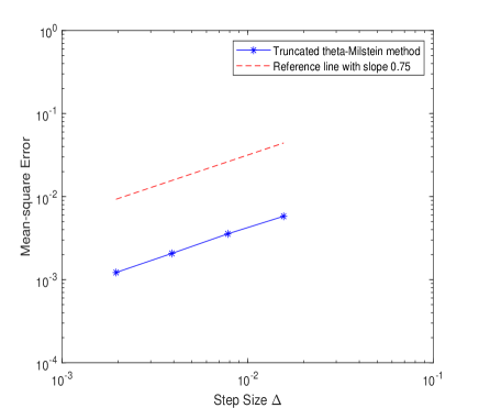
Figure 1: The convergence rate of the truncated $\theta$-Milstein method for (4.1).

Note that we cannot give the explicit form of the true solution. In the numerical experiment, we view the truncated $\theta$-Milstein method with the smallest step size ($2^{-11}$) as the true solution. Two thousand sample paths are simulated. Figure 1 gives the $\mathcal{L}^{2}$-errors defined by

$$(\mathbb{E}|x(T)-\eta_{\Delta}(T)|^{2})^{\frac{1}{2}}\approx\left(\frac{1}{2000}\sum_{i=1}^{2000}|x^{i}(T)-\eta^{i}_{\Delta}(T)|^{2}\right)^{\frac{1}{2}},$$

with step sizes $2^{-9}$, $2^{-8}$, $2^{-7}$, $2^{-6}$ at $T=1$. From Figure 1, we can observe that the convergence rate of the truncated $\theta$-Milstein method for (4.1) is approximately 0.75, which implies that the theoretical results are reliable.

Remark 5.

When delay is vanishing (i.e., $\tau=0$), SDDE (4.1) will degenerate into nonautonomous SDE. The research about the explicit TMM (i.e., $\theta=0$) for nonautonomous SDEs can be found in [23].

5 Conclusion and future research

In this work, we establish the truncated $\theta$-Milstein method for a class of nonautonomous and highly nonlinear SDDEs which have practical applications in many fields. The convergence rate is investigated in $\mathcal{L}^{\bar{q}}(\bar{q}\geq 2)$ sense under the weaker conditions than the existing results. An example and its numerical simulation are presented to show the effectiveness of the truncated $\theta$-Milstein method.

The future work is to analyze the long-time asymptotic behavior of the truncated $\theta$-Milstein method for SDDE (2.1). Additionally, investigating the stability of the truncated $\theta$-Milstein method for SDDE (2.1) by adjusting the parameter $\theta$ is meaningful to us.

References

- [1] E. Allen, Modeling with Itô Stochastic Differential Equations, Springer, Dordrecht, 2007.
- [2] A. Ambrosetti, G. Prodi, A Primer of Nonlinear Analysis, Vol. 34, in: Cambridge Studies in Advanced Mathematics, Cambridge University Press, Cambridge, 1993.
- [3] J.A.D. Appleby, M. Guzowska, C. Kelly, A. Rodkina, Preserving positivity in solutions of discretised stochastic differential equations, Appl. Math. Comput. 217 (2010) 763-774.
- [4] L. Arnold, Stochastic Differential Equations: Theory and Applications, John Wiley, New York, 1974.
- [5] C.T.H. Baker, E. Buckwar, Numerical analysis of explicit one-step methods for stochastic delay differential equations, J. Comput. Math. 3 (2000) 315-335.
- [6] J. Bao, B. Böttcher, X. Mao, C. Yuan, Convergence rate of numerical solutions to SFDEs with jumps, J. Comput. Appl. Math. 236 (2) (2011) 119-131.
- [7] A. Calzolari, P. Florchinger, G. Nappo, Nonlinear filtering for stochastic systems with fixed delay: Approximation by a modified Milstein scheme, Comput. Math. Appl. 61 (2011) 2498-2509.
- [8] S. Deng, W. Fei, W. Liu, X. Mao, The truncated EM method for stochastic differential equations with Poisson jumps, J. Comput. Appl. Math. 355 (2019) 232-257.
- [9] W. Fei, L. Hu, X. Mao, D. Xia. Advances in the truncated Euler-Maruyama method for stochastic differential delay equations, Commun. Pure Appl. Anal. 19 (4) (2020) 2081-2100.
- [10] S. Gao, J. Hu, L. Tan, C. Yuan, Strong convergence rate of truncated Euler-Maruyama method for stochastic differential delay equations with Poisson jumps, Front. Math. China 16, (2021) 395-423.
- [11] Q. Guo, W. Liu, X. Mao, R. Yue, The partially truncated Euler-Maruyama method and its stability and boundedness, Appl. Numer. Math. 115 (2017) 235-251.
- [12] Q. Guo, W. Liu, X. Mao, R. Yue, The truncated Milstein method for stochastic differential equations with commutative noise, J. Comput. Appl. Math. 338 (2018) 298-310.
- [13] Q. Guo, X. Mao, R. Yue, The truncated Euler-Maruyama method for stochastic differential delay equations. Numer. Algorithms. 78 (2) (2018) 599-624.
- [14] D.J. Higham, X. Mao, A.M. Stuart, Strong convergence of Euler-type methods for nonlinear stochastic differential equations, SIAM J. Numer. Anal. 40 (3) (2002) 1041-1063.
- [15] L. Hu, X. Li, X. Mao, Convergence rate and stability of the truncated Euler-Maruyama method for stochastic differential equations, J. Comput. Appl. Math. 337 (2018) 274-289.
- [16] Y. Hu, S.E.A. Mohammed, F. Yan, Discrete-time approximations of stochastic delay equations: the Milstein Scheme, Ann. Probab. 32 (2004) 265-314.
- [17] N. Hofmann, T. Müller-Gronbach, A modified Milstein scheme for approximation of stochastic delay differential equations with constant time lag, J. Comput. Appl. Math. 197 (2006) 89-121.
- [18] M. Hutzenthaler, A. Jentzen, P.E. Kloeden, Strong and weak divergence in finite time of Euler’s method for stochastic differential equations with non-globally Lipschitz continuous coefficients, Proc. R. Soc. A. 467 (2011) 1563-1576.
- [19] M. Hutzenthaler, A. Jentzen, P.E. Kloeden, Strong convergence of an explicit numerical method for SDEs with nonglobally Lipschitz continuous coefficients, Ann. Appl. Probab. 22 (4) (2012) 1611-1641.
- [20] P.E. Kloeden, E. Platen, Numerical Solution of Stochastic Differential Equations, Springer, Berlin, 1992.
- [21] P.E. Kloeden, T. Shardlow, The Milstein scheme for stochastic delay differential equations without using anticipative calculus, J. Sto. Anal. Appl. 30 (2) (2012) 181-202.
- [22] X. Li, X. Mao, G. Yin, Explicit numerical approximations for stochastic differential equations in finite and infinite horizons: truncation methods, convergence in pth moment and stability, IMA J. Numer. Anal. 39 (2019) 847-892.
- [23] J. Liao, W. Liu, X. Wang, Truncated Milstein method for non-autonomous stochastic differential equations and its modification, J. Comput. Appl. Math. 402 (2022) 113817.
- [24] M. Liu, W. Cao, Z. Fan, Convergence and stability of the semi-implicit Euler method for a linear stochastic differential delay equation, J. Comput. Appl. Math. 170 (2004) 255-268.
- [25] W. Liu, X. Mao, J. Tang, Y. Wu, Truncated Euler-Maruyama method for classical and time-changed non-autonomous stochastic differential equations, Appl. Numer. Math. 153 (2020) 66-81.
- [26] W. Mao, Q. Zhu, X. Mao, Existence, uniqueness and almost surely asymptotic estimations of the solutions to neutral stochastic functional differential equations driven by pure jumps, Appl. Math. Comput. 254 (2015) 252-265.
- [27] X. Mao, Stochastic Differential Equations and Applications, 2nd ed. Horwood, Chichester, 2007.
- [28] X. Mao, Numerical solutions of stochastic differential delay equations under the generalized Khasminskii-type conditions, Appl. Math. Comput. 217 (12) (2011) 5512-5524.
- [29] X. Mao, The truncated Euler-Maruyama method for stochastic differential equations, J. Comput. Appl. Math. 290 (2015) 370-384.
- [30] X. Mao, Convergence rates of the truncated Euler-Maruyama method for stochastic differential equations, J. Comput. Appl. Math 296 (2016) 362-375.
- [31] X. Mao, C. Yuan, Stochastic Differential Equations with Markovian Switching, Imperial College Press, 2006.
- [32] G.N. Milstein, E. Platen, H. Schurz, Balanced implicit methods for stiff stochastic system, SIAM J. Numer. Anal. 35 (1998) 1010-1019.
- [33] O.F. Rouz, D. Ahmadian, M. Milev, Exponential mean-square stability of two classes of theta Milstein methods for stochastic delay differential equations, AIP Conf. Proc. 1910 (1) (2017) 060015.
- [34] S. Sabanis, A note on tamed Euler approximations, Electron. Commun. Probab. 18 (2013) 1-10.
- [35] G. Song, J. Hu, S. Gao, X. Li, The strong convergence and stability of explicit approximations for nonlinear stochastic delay differential equations, Numer. Algorithms. (2021).
- [36] M. Song, L. Hu, X. Mao, L. Zhang, Khasminskii-type theorems for stochastic functional differential equations, Discrete Contin. Dyn. Syst. Ser. B 6 (6) (2013) 1697-1714.
- [37] X. Wang, S. Gan, The improved split-step backward Euler method for stochastic differential delay equations, Int. J. Comput. Math. 88 (11) (2011) 2359-2378.
- [38] X. Wang, S. Gan, The tamed Milstein method for commutative stochastic differential equations with non-globally Lipschitz continuous coefficients, J. Differ. Equ. Appl. 19 (3) (2013) 466-490.
- [39] Z. Wang, C. Zhang, An analysis of stability of milstein method for stochastic differential equations with delay, Comput. Math. Appl. 51 (2006) 1445-1452.
- [40] E. Zeidler, Nonlinear functional analysis and its applications, Springer New York, New York, 1990.
- [41] W. Zhang, M. Song, M. Liu, Strong convergence of the partially truncated Euler-Maruyama method for a class of stochastic differential delay equations, J. Comput. Appl. Math. 335 (2018) 114-128.
- [42] W. Zhang, X. Yin, M. Song, M. Liu, Convergence rate of the truncated Milstein method of stochastic differential delay equations, Appl. Math. Comput. 357 (2019) 263-281.
- [43] Y. Zhang, M. Song, M. Liu, Convergence and stability of stochastic theta method for nonlinear stochastic differential equations with piecewise continuous arguments, J. Comput. Appl. Math. 403 (2022) 113849.
- [44] G. Zhao, M. Liu, Numerical methods for nonlinear stochastic delay differential equations with jumps, Appl. Math. Comput. 233 (2014) 222-231.
- [45] X. Zong, F. Wu, G. Xu, Convergence and stability of two classes of theta-Milstein schemes for stochastic differential equations, J. Comput. Appl. Math. 336 (2018) 8-29.