Inferring nonequilibrium thermodynamics from tilted equilibrium
using information-geometric Legendre transform

Abstract

Nonstationary thermodynamic quantities depend on the full details of nonstationary probability distributions, making them difficult to measure directly in experiments or numerics. We propose a method to infer thermodynamic quantities in relaxation processes by measuring only a few observables, using additional information obtained from measurements in tilted equilibrium, i.e., equilibrium with external fields applied. Our method is applicable to arbitrary classical stochastic systems, possibly underdamped, that relax to equilibrium. The method allows us to compute the exact value of the minimum entropy production (EP) compatible with the nonstationary observations, giving a tight lower bound on the true EP. Under a certain additional condition, it also allows the inference of the EP rate, thermodynamic forces, and a new constraint on relaxation paths. Our method is based on a newly developed Legendre transform at the level of probability distributions that originates from information geometry.

Introduction

Relaxation processes are ubiquitous in nature, which experience various nonstationary probability distributions before relaxing to the final stationary distribution. For example, biological systems such as biochemical signaling pathways [1, 2] and neurons [3, 4] respond to external signals in a transient manner to convey information. Relaxation processes also include various nontrivial physical phenomena, such as nonmonotonic relaxations [5, 6, 7], slow glassy relaxations [8], and sudden “cutoff” relaxations [9, 10].

These processes are out of equilibrium and thus have inevitable thermodynamic costs. According to stochastic thermodynamics [11, 12, 13], thermodynamic costs such as EP and thermodynamic forces depend on the full details of nonstationary probability distributions. Therefore, in order to obtain thermodynamic quantities directly in experiments or numerical simulations, we need to measure all the details of probability distributions by accumulating many realizations of the same relaxation process and computing the histogram at each time point. This nonstationary measurement is practically impossible for systems with more than a few states.

To reduce the demand for nonstationary measurements, we need to develop indirect methods to infer thermodynamic quantities from measurable partial information. Such methods have been actively studied in stochastic thermodynamics, collectively referred to as thermodynamic inference [14]. Previous studies have used various types of measurable partial information, such as raw time series data [15, 16, 17], correlation and response functions [18, 19], coarse-grained states [20, 21, 22, 23], partial transitions [24, 25, 26], current observables [27, 28], mean local velocities [29, 30, 31], arbitrarily weighted local currents [32, 33, 34, 35, 36, 37, 38, 39, 40], sojourn probabilities of tubular paths [41], the Fisher information [42], and waiting time distributions of transitions [43, 44, 45, 46], to infer thermodynamic quantities such as the EP rate. However, most of these studies are concerned with steady states, and only a few of them develop thermodynamic inference methods for nonstationary processes [24, 39, 40, 41]. Moreover, existing methods for nonstationary processes rely only on nonstationary measurements, thus imposing a relatively high demand for nonstationary data. It is natural to ask whether we can reduce the required nonstationary data by using additional data from other types of measurements.

In this paper, we propose a new approach to the thermodynamic inference for relaxation processes: inferring thermodynamic quantities from “tilted equilibrium,” i.e., the equilibrium under the application of external fields to the system. Our approach combines the nonstationary measurement of a few observables with the tilted equilibrium measurement of the same set of observables. From these data, our method allows us to compute the exact value of the minimum EP compatible with the nonstationary data, which constitutes a tight lower bound on the true EP over the relaxation from any intermediate distribution to the final equilibrium. Moreover, if the system satisfies a condition called realizability condition, which says that the nonstationary distribution is exactly realized as a tilted equilibrium, our method provides us with additional information about the process: the exact value of the true EP, the instantaneous EP rate, the nonstationary thermodynamic forces, and a new constraint on relaxation trajectories. Our method applies to arbitrary classical stochastic systems, including overdamped and underdamped systems, that may have continuous or discrete state spaces, as long as they relax to equilibrium.

This paper is organized as follows. In Sec. II, we state the setup and define the problem. Sec. III is the main section of this paper, where we introduce the tilted equilibrium measurements and establish the inference method of the minimum EP. In Sec. IV, we numerically demonstrate our proposed method with a one-dimensional Brownian particle. Sec. V develops additional inference methods under the realizability condition. In Sec. VI, we sketch the derivation of the results. The derivation involves a new Legendre transform at the level of probability distributions developed based on a similar Legendre transform in information geometry [47, 48]. Formal aspects of this new Legendre transform will be detailed in a separate paper [49]. Sec. VII concludes the paper.

Nonequilibrium thermodynamics

Setup

We consider a stochastic system in contact with a single heat bath at a constant temperature $T$. The system stochastically moves around a continuous state space $\mathcal{X}\subset\mathbb{R}^{d}$ or a discrete state space $\mathcal{X}\coloneqq\{1,\dots,N\}$. Let $p(x)$ denote a probability density function for a continuous system and a probability mass function for a discrete case, which satisfies $\int_{\mathcal{X}}dx\,p(x)=1$. Here and hereafter, $\int_{\mathcal{X}}dx$ should always be replaced by $\sum_{x\in\mathcal{X}}$ for discrete cases. The system in state $x$ has energy $\epsilon(x)$, which is assumed to be time-independent. The state energy determines the equilibrium distribution $p_{\mathrm{eq}}\equiv\{p_{\mathrm{eq}}(x)\}_{x\in\mathcal{X}}$ with $p_{\mathrm{eq}}(x)\propto\exp[-\epsilon(x)/k_{\text{b}}T]$, where $k_{\text{b}}$ is the Boltzmann constant.

The system exhibits a relaxation process ${\tilde{p}}(t)\equiv\{{\tilde{p}}(x;t)\}_{x\in\mathcal{X}}$ for $t\geq 0$, where $t$ is the time variable. For notational convenience, we use tilde ($\tilde{\phantom{\,\cdot\,}}$) for quantities associated with the relaxation process of interest. We assume that the process ${\tilde{p}}(t)$ converges to the equilibrium distribution, ${\tilde{p}}(t)\to p_{\mathrm{eq}}$ as $t\to\infty$. We do not assume any specific time evolution law unless otherwise noted.

The fundamental assumption of this paper is that the details of ${\tilde{p}}(x;t)$ are not measurable, but we can measure the expectation values of a few observables $B_{1},\dots,B_{K}$. The number $K\geq 1$ is arbitrary, and we have in mind in particular a small number such as 2 or 3. An observable $B_{\alpha}\equiv\{B_{\alpha}(x)\}_{x\in\mathcal{X}}$ is any real-valued function over $\mathcal{X}$, and its expectation value over a probability distribution $p$ is $\langle B_{\alpha}\rangle_{p}\coloneqq\int_{\mathcal{X}}dx\,B_{\alpha}(x)p(x)$. We use the notation $\bm{B}\equiv(B_{1},\dots,B_{K})^{\mathsf{T}}$ and $\langle\bm{B}\rangle_{p}\equiv(\langle B_{1}\rangle_{p},\cdots,\langle B_{K}\rangle_{p})^{\mathsf{T}}$. Without loss of generality, we assume that the $K$ observables are linearly independent of each other. We also assume that the $K$ observables are linearly independent with a constant observable (a trivial observable whose value does not depend on $x$) because such an observable gives no information about the process. We write the set of expectation values measured at time $t$ as

$${\tilde{\bm{\eta}}}(t)\coloneqq\langle\bm{B}\rangle_{{\tilde{p}}(t)},$$ (1)

which is the only nonstationary data needed for our proposed method [Fig. 1(a)].

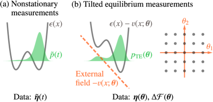
Figure 1: Schematics of the proposed inference method. (a) A system undergoing a relaxation process with a time-independent energy $\epsilon(x)$ and a nonstationary distribution ${\tilde{p}}(t)$. Our method requires only the data of the expectation values of a few observables, ${\tilde{\bm{\eta}}}(t)=\langle\bm{B}\rangle_{{\tilde{p}}(t)}$, along the process. (b) To systematically collect data from tilted equilibrium measurements, we apply the external field $v(x;\bm{\theta})$ and measure the expectation values of the observables, $\bm{\eta}(\bm{\theta})=\langle\bm{B}\rangle_{p_{\scriptstyle\text{te}}(\bm{\theta})}$, for many $\bm{\theta}$’s. We also compute the tilted equilibrium free energy $\Delta{\mathcal{F}}(\bm{\theta})$ from the measured values of $\bm{\eta}(\bm{\theta})$.

EP and the minimum EP

The fundamental quantity characterizing the thermodynamic cost of a relaxation process is the EP [12]. For systems in contact with a single heat bath, the EP of the relaxation process from ${\tilde{p}}(t)$ to $p_{\mathrm{eq}}$ is given by $T^{-1}\Delta{\mathcal{H}}[{\tilde{p}}(t)]$, where

$${\mathcal{H}}[p]\coloneqq k_{\text{b}}T\!\int_{\mathcal{X}}dx\,p(x)\ln p(x)+\int_{\mathcal{X}}dx\,\epsilon(x)p(x)$$ (2)

and $\Delta{\mathcal{H}}[p]\coloneqq{\mathcal{H}}[p]-{\mathcal{H}}[p_{\mathrm{eq}}]$ [12, 50]. The first term in Eq. (2) accounts for the change in the Shannon entropy of the system, while the second term gives the change in the bath entropy due to heat flux. Since $T$ is set constant throughout the paper, we abuse terminology and call $\Delta{\mathcal{H}}[{\tilde{p}}(t)]$ the EP. The EP depends on the details of the probability distribution, and we need ${\tilde{p}}(x;t)$ for all $x$ and all $t$ if we want to compute $\Delta{\mathcal{H}}[{\tilde{p}}(t)]$ directly from Eq. (2).

Since the measured data ${\tilde{\bm{\eta}}}(t)$ is not sufficient to determine a single value of $\Delta{\mathcal{H}}[{\tilde{p}}(t)]$, we follow the general concept in Ref. [23] to focus on the range of EP compatible with the data ${\tilde{\bm{\eta}}}(t)$. There is no upper limit of the compatible range because hidden (unobserved) degrees of freedom can cause an arbitrarily large EP [21]. On the other hand, there is a lower bound, which we write as

$$\Delta{\mathcal{H}_{\mathrm{m}}}(\bm{\eta})\coloneqq\min_{\left.q\;\middle|\,\langle\bm{B}\rangle_{q}=\bm{\eta}\right.}\Delta{\mathcal{H}}[q]$$ (3)

for any set of expectation values $\bm{\eta}$. Here, the minimum is taken over all probability distributions $q$ that satisfy $\langle\bm{B}\rangle_{q}\nobreak=\nobreak\bm{\eta}$, i.e., that are compatible with the set of expectation values $\bm{\eta}$. Since $\Delta{\mathcal{H}}[q]$ is the dissipation of the relaxation process from $q$ to $p_{\mathrm{eq}}$, any relaxation process that exhibits the set of expectation values $\bm{\eta}$ at some point in time must dissipate at least $\Delta{\mathcal{H}_{\mathrm{m}}}(\bm{\eta})$ before relaxing to the final equilibrium. For this reason, $\Delta{\mathcal{H}_{\mathrm{m}}}(\bm{\eta})$ is interpreted as the fundamental cost associated with the set of expectation values $\bm{\eta}$.

Thermodynamic inference

Tilted equilibrium

Our main result is a method for calculating the minimum EP $\Delta{\mathcal{H}_{\mathrm{m}}}(\bm{\eta})$ from tilted equilibrium measurements. The method uses a family of external fields parameterized by $\bm{\theta}=(\theta_{1},\dots,\theta_{K})^{\mathsf{T}}$:

$$v(x;\bm{\theta})=\sum_{\alpha=1}^{K}\theta_{\alpha}B_{\alpha}(x).$$ (4)

In words, the external field $v(x;\bm{\theta})$ is the superposition of the fields conjugate to the observable $B_{\alpha}$ with an intensity $\theta_{\alpha}$. The external field $v(x;\bm{\theta})$ incurs the tilted equilibrium $p_{\scriptstyle\text{te}}(\bm{\theta})\equiv\{p_{\scriptstyle\text{te}}(x;\bm{\theta})\}_{x\in\mathcal{X}}$ with

$$p_{\scriptstyle\text{te}}(x;\bm{\theta})\propto\exp\quantity(-\frac{\epsilon(x)-v(x;\bm{\theta})}{k_{\text{b}}T})\,.$$ (5)

Here, we use the convention for the sign of the external field such that it modifies the state energy from $\epsilon(x)$ to $\epsilon(x)-v(x;\bm{\theta})$.

We propose the following procedure for collecting tilted equilibrium data to perform the thermodynamic inference systematically [Fig. 1(b)]:

1. Realize the tilted equilibrium distributions for sufficiently many sets of parameter values $\bm{\theta}$, and measure the expectation values of the observables $\bm{B}$,

   $$\bm{\eta}(\bm{\theta})\coloneqq\langle\bm{B}\rangle_{p_{\scriptstyle\text{te}}(\bm{\theta})},$$ (6)

   for each $\bm{\theta}$.

2. Interpolate the measured expectation values to infer the functional dependence $\bm{\eta}(\bm{\theta})$ over a range of $\bm{\theta}$.

3. Calculate the tilted equilibrium free energy $\Delta{\mathcal{F}}(\bm{\theta})$ from the data $\bm{\eta}(\bm{\theta})$ as described below.

The tilted equilibrium free energy is defined as

$${\mathcal{F}}(\bm{\theta})\coloneqq-k_{\text{b}}T\ln\left[\int_{\mathcal{X}}dx\exp\left(-\frac{\epsilon(x)-v(x;\bm{\theta})}{k_{\text{b}}T}\right)\right],$$ (7)

and $\Delta{\mathcal{F}}(\bm{\theta})\coloneqq{\mathcal{F}}(\bm{\theta})-{\mathcal{F}}(\bm{0})$. The difference $\Delta{\mathcal{F}}(\bm{\theta})$ is computed from the data $\bm{\eta}(\bm{\theta})$ as (see Sec. VI.1 for derivation)

$$\Delta{\mathcal{F}}(\bm{\theta})=-\int_{\bm{0}}^{\bm{\theta}}\bm{\eta}(\bm{\theta}^{\prime})\cdot d\bm{\theta}^{\prime},$$ (8)

where the line integral is over any curve connecting $\bm{\theta}^{\prime}=\bm{0}$ and $\bm{\theta}^{\prime}=\bm{\theta}$, and the resulting value does not depend on the intermediate path.

As we show in Sec. VI.1, the correspondence from $\bm{\theta}$ to $\bm{\eta}$, denoted by $\bm{\eta}(\bm{\theta})$ in Eq. (6), is invertible. We write the inverse function as $\bm{\theta}(\bm{\eta})$, which solves

$$\langle\bm{B}\rangle_{p_{\scriptstyle\text{te}}(\bm{\theta}(\bm{\eta}))}=\bm{\eta}$$ (9)

for each $\bm{\eta}$. In other words, $\bm{\theta}(\bm{\eta})$ is the unique set of parameter values that incurs the set of expectation values $\bm{\eta}$. Using the interpolated data of $\bm{\eta}(\bm{\theta})$, one can find $\bm{\theta}(\bm{\eta})$ for a given $\bm{\eta}$ if the data range covers the given $\bm{\eta}$. For simplicity, we assume that the data range is large enough to cover any $\bm{\eta}$ that appears below.

In summary, we have the data of $\bm{\eta}(\bm{\theta})$ and $\Delta{\mathcal{F}}(\bm{\theta})$ from the tilted equilibrium measurements, and when a set of expectation values $\bm{\eta}$ is given, we can find $\bm{\theta}(\bm{\eta})$ from the tilted equilibrium data.

Inference of minimum EP

In terms of these tilted equilibrium data, the minimum EP (3) is expressed as

$$\Delta{\mathcal{H}_{\mathrm{m}}}(\bm{\eta})=\Delta{\mathcal{F}}(\bm{\theta}(\bm{\eta}))+\sum_{\alpha=1}^{K}\theta_{\alpha}(\bm{\eta})\,\eta_{\alpha},$$ (10)

which is the central relation of our inference method. We can calculate the right-hand side of Eq. (10) for a given $\bm{\eta}$ from the tilted equilibrium data. To do so, we first find $\bm{\theta}(\bm{\eta})$, i.e., the set of parameter values corresponding to the given $\bm{\eta}$, from the interpolated data $\bm{\eta}(\bm{\theta})$. Then, we look up the value of the tilted equilibrium free energy $\Delta{\mathcal{F}}(\bm{\theta}(\bm{\eta}))$. Equation (10) is derived in Sec. VI.1 and Appendix B.

From Eq. (1) and the definition of $\Delta{\mathcal{H}_{\mathrm{m}}}(\bm{\eta})$ in Eq. (3), the true EP of the process for each $t$ is lower bounded as

$$\Delta{\mathcal{H}}[{\tilde{p}}(t)] \geq\Delta{\mathcal{H}_{\mathrm{m}}}({\tilde{\bm{\eta}}}(t))$$ (11a)

$$=\Delta{\mathcal{F}}(\bm{\theta}({\tilde{\bm{\eta}}}(t)))+\sum_{\alpha=1}^{K}\theta_{\alpha}({\tilde{\bm{\eta}}}(t))\,\tilde{\eta}_{\alpha}(t).$$ (11b)

The expression (11b) can be calculated by combining the nonstationary data and the tilted equilibrium data. To do so, we first use the tilted equilibrium data to find $\bm{\theta}({\tilde{\bm{\eta}}}(t))$, i.e., the set of parameter values that incurs the same set of expectation values as the nonstationary data ${\tilde{\bm{\eta}}}(t)$. Then, we find the value of the tilted equilibrium free energy $\Delta{\mathcal{F}}(\bm{\theta}({\tilde{\bm{\eta}}}(t)))$. We emphasize that the calculated value of $\Delta{\mathcal{H}_{\mathrm{m}}}({\tilde{\bm{\eta}}}(t))$ is not merely a lower bound on the true EP but a meaningful thermodynamic cost. Indeed, it is the fundamental cost for producing the observed set of expectation values ${\tilde{\bm{\eta}}}(t)$ in relaxation processes, as discussed below Eq. (3).

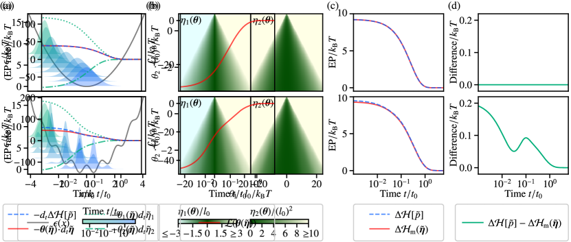
Figure 2: Demonstration of our inference method with a one-dimensional Brownian particle with $\epsilon(x)=ax^{2}+b\cos cx$. The upper panels are with $b=0$ (harmonic), and the lower panels are with $b=k_{\text{b}}T$ (ragged). We scale the energy by $k_{\text{b}}T$, the length by $l_{0}\coloneqq\sqrt{k_{\text{b}}T/a}$, and the time by $t_{0}\coloneqq 1/a\mu$, where $\mu$ is the mobility. See main text for parameter values. (a) The potential energy $\epsilon(x)$ (gray) and the probability distributions over a relaxation process (blue; vertically shifted), which are assumed to be unmeasurable. (b) The tilted equilibrium measurement measures the expectation values of the observables $(\eta_{1}(\bm{\theta}),\eta_{2}(\bm{\theta}))$ with varying the external field parameters $\bm{\theta}\equiv(\theta_{1},\theta_{2})$. (c) Inference of the minimum EP. The minimum EP $\Delta{\mathcal{H}_{\mathrm{m}}}({\tilde{\bm{\eta}}}(t))$ is obtained from the measurements (red), while the true EP $\Delta{\mathcal{H}}[{\tilde{p}}(t)]$ is not measurable (blue). (d) The difference between the true EP and the obtained minimum EP, $\Delta{\mathcal{H}}[{\tilde{p}}(t)]-\Delta{\mathcal{H}_{\mathrm{m}}}({\tilde{\bm{\eta}}}(t))$.

Equality condition and tightness

If the inequality (11a) holds with equality, we can use Eq. (11b) to calculate the exact value of the true EP from the nonstationary and tilted equilibrium data. As shown in Sec. VI.2, this happens if and only if

$$\exists\,\bm{\theta},\quad{\tilde{p}}(t)=p_{\scriptstyle\text{te}}(\bm{\theta}),$$ (12)

namely, ${\tilde{p}}(t)$ is exactly realizable as a tilted equilibrium. We call the condition (12) realizability condition. We discuss when the realizability condition holds in Sec. V.1.

Apart from the equality condition, we make two remarks about the tightness of the inequality (11a). First, the inequality (11a) becomes tighter as we increase $K$ by adding more observables to $\bm{B}$. This is because increasing $K$ has the effect of narrowing the domain of minimization in Eq. (3) and raising the minimum EP $\Delta{\mathcal{H}_{\mathrm{m}}}(\bm{\eta})$.

Second, we can sometimes get a tighter bound by considering the whole process at once, assuming that the time evolution is Markovian:

$$\Delta{\mathcal{H}}[{\tilde{p}}(t)]=\max_{t^{\prime}\,|\,t^{\prime}\geq t}\Delta{\mathcal{H}}[{\tilde{p}}(t^{\prime})]\geq\max_{t^{\prime}\,|\,t^{\prime}\geq t}\Delta{\mathcal{H}_{\mathrm{m}}}({\tilde{\bm{\eta}}}(t^{\prime})).$$ (13)

The first equality is the second law of thermodynamics for the true EP, $-d_{t}\Delta{\mathcal{H}}[{\tilde{p}}(t)]\geq 0$, where $d_{t}\equiv d/dt$ is the time derivative, which holds under the Markovian assumption [12, 51]. The second inequality follows from the inequality (11a). The last side of Eq. (13) can be computed from the considered data using Eq. (11b), and it gives a tighter bound than Eq. (11a) if $\Delta{\mathcal{H}_{\mathrm{m}}}({\tilde{\bm{\eta}}}(t))$ is not monotonically decreasing in time.

Example: Trapped Brownian particle

Model and required measurements

We demonstrate our results with a one-dimensional Brownian particle in a harmonic trapping potential plus a ragged potential,

$$\epsilon(x)=ax^{2}+\epsilon_{r}(x),$$ (14)

where $a>0$ determines the width of the harmonic potential, and $\epsilon_{r}(x)$ is an arbitrary ragged potential. It is a model of an optically trapped particle linked to a biomolecule [52, 12], for which $\epsilon_{r}(x)$ denotes the energy of the biomolecule pulled to a displacement $x$. The time evolution is governed by the Fokker–Planck equation with a uniform mobility $\mu$, $\partial_{t}{\tilde{p}}(x;t)=\mu\partial_{x}[{\tilde{p}}(x;t)\partial_{x}\epsilon(x)+k_{\text{b}}T\partial_{x}{\tilde{p}}(x;t)]$, where $\partial_{t}\equiv\partial/\partial t$ and $\partial_{x}\equiv\partial/\partial x$ denote the time and spatial derivatives.

As an example, we consider the case where we can keep track of the mean and variance of the position $x$ of the particle over relaxation processes, but we cannot reliably get the higher moments due to the limited number of relaxation trajectories obtained from experiments. This assumption corresponds to the choice of two observables, $B_{1}(x)=x$ and $B_{2}(x)=x^{2}$, in our framework. To perform the tilted equilibrium measurements, we need to modify the energy to

$$\epsilon(x)-v(x;\bm{\theta})=(a-\theta_{2})x^{2}-\theta_{1}x+\epsilon_{r}(x),$$ (15)

which is still a harmonic potential plus the ragged potential. Therefore, we can realize the tilted equilibrium by modulating the center and the width of the harmonic trapping potential. We need to measure the mean and variance of the position $x$ at many tilted equilibrium distributions, interpolate the data to find $\bm{\eta}(\bm{\theta})$, and compute $\Delta{\mathcal{F}}(\bm{\theta})$ as described in Sec. III.1.

If $\epsilon_{r}(x)=0$ and the initial distribution is Gaussian, the realizability condition (12) holds. To see this, we first note that ${\tilde{p}}(t)$ is Gaussian for all $t\geq 0$ for a Gaussian initial distribution [53]. Since we can make any harmonic potential by changing $\theta_{1}$ and $\theta_{2}$ in Eq. (15) for $\epsilon_{r}(x)=0$, we can realize any Gaussian distribution as a tilted equilibrium. Therefore, the realizability condition is satisfied, and the equality holds in Eq. (11a), allowing us to extract the exact value of $\Delta{\mathcal{H}}[{\tilde{p}}(t)]$ from the tilted equilibrium data. In the case of a nonzero ragged potential, the equality condition no longer holds. Nevertheless, if $\epsilon_{r}(x)$ is small enough, we expect that ${\tilde{p}}(t)$ is approximately realizable as a tilted equilibrium distribution, and therefore Eq. (11b) gives a fairly accurate estimate of $\Delta{\mathcal{H}}[{\tilde{p}}(t)]$.

Numerical results

We numerically demonstrate our inference scheme for $\epsilon_{r}(x)=b\cos cx$. In all calculations, we scale the energy by $k_{\text{b}}T$, the length by $l_{0}\coloneqq\sqrt{k_{\text{b}}T/a}$, and the time by $t_{0}\coloneqq 1/a\mu$. We set $b=0$ (harmonic; the upper panels of Fig. 2) or $b=1k_{\text{b}}T$ (ragged; the lower panels of Fig. 2) and $c=6(l_{0})^{-1}$. The initial distribution is the Gaussian distribution with mean $-3l_{0}$ and variance $0.15(l_{0})^{2}$ for all calculations. No other parameters are free to choose after scaling the quantities. See also Appendix E for more details on the numerics.

We plot the potential $\epsilon(x)$ and the time evolution ${\tilde{p}}(t)$, both assumed to be unmeasurable, in Fig. 2(a). The ragged system has potential barriers that separate the state space into metastable wells. Figure 2(b) shows the tilted equilibrium data $\bm{\eta}(\bm{\theta})$. In the ragged system, $\bm{\eta}(\bm{\theta})$ has a step-like feature, reflecting the multi-well structure of the potential. We sampled $\bm{\eta}(\bm{\theta})$ from sufficiently dense data points over the $\bm{\theta}$ space, leaving the consideration of sparse data points to future work.

Figure 2(c) shows the minimum EP $\Delta{\mathcal{H}_{\mathrm{m}}}({\tilde{\bm{\eta}}}(t))$ compatible with the observed mean and variance, which is calculated using the tilted equilibrium data via Eq. (11b). The true EP $\Delta{\mathcal{H}}[{\tilde{p}}(t)]$ is also plotted, which is not measurable. The figure shows that the calculated value $\Delta{\mathcal{H}_{\mathrm{m}}}({\tilde{\bm{\eta}}}(t))$ is equal to or less than the true EP $\Delta{\mathcal{H}}[{\tilde{p}}(t)]$, thus confirming the inequality (11a). Moreover, these two quantities agree exactly for $b=0$, and they are in fairly good agreement for $b=1k_{\text{b}}T$ [Fig. 2(d)]. The former is expected from the realizability condition, as discussed in Sec. IV.1. The latter, in contrast, is rather surprising because the height of the ragged potential is $2b=2k_{\text{b}}T$, which is not very small compared to $k_{\text{b}}T$. This example shows that, even if the realizability condition is violated, the minimum EP can be a good approximation of the true EP.

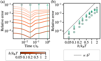
Figure 3: Relative error, $\{\Delta{\mathcal{H}}[{\tilde{p}}(t)]-\Delta{\mathcal{H}_{\mathrm{m}}}({\tilde{\bm{\eta}}}(t))\}/\Delta{\mathcal{H}}[{\tilde{p}}(t)]$, between the true EP and the calculated minimum EP. (a) Relative error over time, plotted for several values of the height $b$ of the ragged potential. (b) Relative error over $b$, plotted for four time points. Each symbol represents a time point indicated in panel (a). The relative error grows quadratically in $b$ (dashed line).

We also present an extensive result over a wide range of $b$. Figure 3(a) shows the relative error, $\bigl{\{}\Delta{\mathcal{H}}[{\tilde{p}}(t)]-\Delta{\mathcal{H}_{\mathrm{m}}}({\tilde{\bm{\eta}}}(t))\bigr{\}}/\Delta{\mathcal{H}}[{\tilde{p}}(t)]$, for various values of $b$. The relative error is zero for $b=0$ due to the realizability condition, and it increases with $b$. It does not significantly depend on $t$. As shown in Fig. 3(b), the relative error for a fixed $t$ scales quadratically in $b$. Therefore, the calculated value $\Delta{\mathcal{H}_{\mathrm{m}}}({\tilde{\bm{\eta}}}(t))$ equals the true EP $\Delta{\mathcal{H}}[{\tilde{p}}(t)]$ up to the first order in $b$. In fact, this quadratic dependence is a generic property, as discussed in Sec. VI.2.

Realizability condition and additional inference methods

As discussed in Sec. III.3, the realizability condition (12) ensures that the inequality (11a) holds with equality, allowing the inference of the exact value of EP. We discuss three situations where the realizability condition is satisfied in Sec. V.1. Moreover, assuming the realizability condition, we can extract additional information about the relaxation process from the tilted equilibrium measurements, including the EP rate, the thermodynamic force, and a new constraint on relaxation paths. We present these additional inference methods in Secs. V.2–V.4.

Sufficient conditions for the realizability condition

There are several physically natural situations in which we can ensure the realizability condition (see Appendix A for details). The first situation is the existence of a time-scale separation. If the states are lumped into groups, the transition rates within a group are sufficiently larger than the rates between different groups, and we can track the total probability of each group, then we can ensure the realizability condition except for the initial fast relaxation. The second situation is when the system admits a symmetry. If the system energy and the time evolution law are symmetric under some permutations of the discrete states, the initial condition has the same symmetry, and we can track all observables obeying the symmetry, then we can ensure the realizability condition. Another situation is when the process is Gaussian. If the state energy is a (possibly multivariate) harmonic potential, the time evolution is described by the Fokker–Planck equation with a uniform mobility, the initial distribution is Gaussian, and we can track the mean and covariance matrix, then the realizability condition holds. This third situation has been demonstrated in the example (Sec. IV). Note that each of these conditions jointly concerns the system energy, the time evolution law, the initial condition, and the choice of observables.

If we have enough information about the system to ensure that the system satisfies one of these sufficient conditions for the realizability condition, we can obtain the exact value of the true EP from Eq. (11b), and we can obtain additional information from the methods described below in Secs. V.2–V.4. Alternatively, if we can expect the system to approximately satisfy one of these sufficient conditions, we expect ${\tilde{p}}(t)$ to be approximately realized as a tilted equilibrium distribution. In this case, $\Delta{\mathcal{H}_{\mathrm{m}}}({\tilde{\bm{\eta}}}(t))$ will be a good approximation of $\Delta{\mathcal{H}}[{\tilde{p}}(t)]$, and the additional inference methods below will provide reasonable estimates of the additional quantities.

EP rate

The first quantity obtained under the realizability condition is the EP rate, ${\tilde{\sigma}}(t)\coloneqq-T^{-1}d_{t}\Delta{\mathcal{H}}[{\tilde{p}}(t)]$. Under the realizability condition, we have the equality $\Delta{\mathcal{H}}[{\tilde{p}}(t)]=\Delta{\mathcal{H}_{\mathrm{m}}}({\tilde{\bm{\eta}}}(t))$, and thus we can obtain the EP rate by simply differentiating $\Delta{\mathcal{H}_{\mathrm{m}}}({\tilde{\bm{\eta}}}(t))$, which is calculated from Eq. (11b). Alternatively, we have the following equality (see Sec. VI.1 for derivation):

$${\tilde{\sigma}}(t)=-\frac{1}{T}d_{t}\Delta{\mathcal{H}_{\mathrm{m}}}({\tilde{\bm{\eta}}}(t))=-\frac{1}{T}\sum_{\alpha=1}^{K}\theta_{\alpha}({\tilde{\bm{\eta}}}(t))\,d_{t}\tilde{\eta}_{\alpha}(t).$$ (16)

The right-hand side of this equation is calculated by differentiating the nonstationary data ${\tilde{\bm{\eta}}}(t)$ and finding $\bm{\theta}({\tilde{\bm{\eta}}}(t))$ from the tilted equilibrium data $\bm{\eta}(\bm{\theta})$.

Equation (16) also provides a decomposition of the EP rate into the dissipation due to the change in the expectation value of each observable. From this equation, we can regard $[-T^{-1}\theta_{\alpha}({\tilde{\bm{\eta}}}(t))]$ as the thermodynamic force conjugate to the probability flux incurring the change in the expectation values $d_{t}\tilde{\eta}_{\alpha}(t)$.

In Fig. 4(a), we demonstrate the inference of the EP rate from Eq. (16) for the same example systems as in Sec. IV. Without a ragged potential (the upper panel), the realizability condition is exactly satisfied, and therefore the right-hand side of Eq. (16) gives the exact value of ${\tilde{\sigma}}(t)$. For a nonzero ragged potential (the lower panel), the realizability condition is approximately satisfied, and indeed the right-hand side of Eq. (16) gives a good estimate of the EP rate.

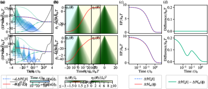
Figure 4: Additional inference under the realizability condition demonstrated with the same systems as in Fig. 2. The harmonic system (upper panels) satisfies the realizability condition, while the ragged system (lower panels) satisfies it only approximately. (a) Inference of the EP rate. The true EP rate $T{\tilde{\sigma}}(t)=-d_{t}\Delta{\mathcal{H}}[{\tilde{p}}(t)]$ (blue) and the obtained estimate $-\bm{\theta}({\tilde{\bm{\eta}}}(t))\cdot d_{t}{\tilde{\bm{\eta}}}(t)$ (red) are in exact agreement under the realizability condition. We also plot the decomposed values $-\theta_{\alpha}({\tilde{\bm{\eta}}}(t))d_{t}\tilde{\eta}_{\alpha}(t)$ (green). (b) New constraint on time evolution. The function $\mathcal{L}(\bm{\theta}({\tilde{\bm{\eta}}}(t)))$ increases monotonically with time under the realizability condition.

Thermodynamic force

The second quantity obtained under the realizability condition is the thermodynamic force (affinity) over the state space. For discrete-state systems, the thermodynamic force from state $y$ to $x$ at time $t$ is given by [50]

$$\tilde{f}(x,y;t)\coloneqq-\frac{\epsilon(x)-\epsilon(y)}{T}-k_{\text{b}}\ln\frac{{\tilde{p}}(x;t)}{{\tilde{p}}(y;t)}.$$ (17)

It is related to the EP rate by ${\tilde{\sigma}}(t)=\frac{1}{2}\sum_{x,y}\tilde{\jmath}(x,y;t)\,\tilde{f}(x,y;t)$, where $\tilde{\jmath}(x,y;t)$ is the net probability flux from state $y$ to $x$ at time $t$ [50]. Thus, the thermodynamic force quantifies the EP rate due to the probability flux from $y$ to $x$. Under the realizability condition, we can calculate the thermodynamic force $\tilde{f}(x,y;t)$ from the considered data as (see Appendix B.4 for derivation)

$$\tilde{f}(x,y;t)=-\frac{1}{T}\sum_{\alpha=1}^{K}\theta_{\alpha}({\tilde{\bm{\eta}}}(t))\,[B_{\alpha}(x)-B_{\alpha}(y)].$$ (18)

The right-hand side can be calculated from the nonstationary data ${\tilde{\bm{\eta}}}(t)$ and the tilted equilibrium data $\bm{\eta}(\bm{\theta})$, assuming that we know the values of the observables $\bm{B}(x)$ in each state.

For continuous-state systems, the thermodynamic force at $x\in\mathbb{R}^{d}$ is defined as a continuous version of Eq. (17) [54], $\tilde{f}(x;t)\coloneqq-T^{-1}\nabla\epsilon(x)-k_{\text{b}}\nabla\ln{\tilde{p}}(x;t)$, which is a $d$-dimensional vector. It is related to the EP rate by ${\tilde{\sigma}}(t)=\int_{\mathcal{X}}dx\,\tilde{\jmath}(x;t)\cdot\tilde{f}(x;t)$, where $\tilde{\jmath}(x;t)$ is the $d$-dimensional probability current at time $t$. We can similarly calculate the thermodynamic force from the data as $\tilde{f}(x;t)=-T^{-1}\sum_{\alpha=1}^{K}\theta_{\alpha}({\tilde{\bm{\eta}}}(t))\nabla B_{\alpha}(x)$ under the realizability condition.

Constraint on the time evolution

The final piece of information obtained from tilted equilibrium measurements is a new constraint on the time evolution. Let us introduce a function of the external field parameters $\bm{\theta}$,

$$\mathcal{L}(\bm{\theta})\coloneqq\Delta{\mathcal{F}}(\bm{\theta})+\sum_{\alpha=1}^{K}\theta_{\alpha}\langle B_{\alpha}\rangle_{p_{\mathrm{eq}}}.$$ (19)

Then, the time evolution of the observables ${\tilde{\bm{\eta}}}(t)$ must satisfy

$$d_{t}\mathcal{L}(\bm{\theta}({\tilde{\bm{\eta}}}(t)))\geq 0,$$ (20)

assuming a Markovian time evolution in addition to the realizability condition (see Appendix B.5 for derivation). This restriction on the possible time trajectories is different from and complementary to the second law of thermodynamics, $-d_{t}\Delta{\mathcal{H}}[{\tilde{p}}(t)]\geq 0$. Note that $\langle B_{\alpha}\rangle_{p_{\mathrm{eq}}}$ is independent of $\bm{\theta}$, and the second term of $\mathcal{L}(\bm{\theta})$ is linear in $\bm{\theta}$. If we shift the definition of each observable by a constant so that $\langle B_{\alpha}\rangle_{p_{\mathrm{eq}}}=0$, $\mathcal{L}(\bm{\theta})$ coincides with $\Delta{\mathcal{F}}(\bm{\theta})$.

In Fig. 4(b), we demonstrate the monotonicity (20) with the same example system as above. For the harmonic system (the upper panel), the realizability condition is satisfied, and the function $\mathcal{L}(\bm{\theta})$ is indeed monotonically increasing. For the ragged system (the lower panel), the realizability condition holds only approximately, but $\mathcal{L}(\bm{\theta})$ is still monotonically increasing.

Derivation

Derivation of the central relation (10)

The derivation of Eq. (10) involves two nontrivial tasks: expressing the minimum EP (3) in a closed form and relating the minimum EP to the tilted equilibrium quantities. We sketch how these two tasks are accomplished, leaving the detailed calculation to Appendix B.

To express the minimum EP in a closed form, we first find the following relation for any set of expectation values $\bm{\eta}$ and any distribution $q$ that satisfies $\langle\bm{B}\rangle_{q}=\bm{\eta}$:

$$\Delta{\mathcal{H}}[q]=k_{\text{b}}TD_{\text{kl}}[q\|p_{\scriptstyle\text{te}}(\bm{\theta}(\bm{\eta}))]+\Delta{\mathcal{H}}[p_{\scriptstyle\text{te}}(\bm{\theta}(\bm{\eta}))],$$ (21)

where $D[p_{1}\|p_{2}]=\int_{\mathcal{X}}dx\,p_{1}(x)\ln[p_{1}(x)/p_{2}(x)]$ is the Kullback–Leibler (KL) divergence [55]. Taking the minimum of both sides of Eq. (21) with respect to $q$ that satisfies $\langle\bm{B}\rangle_{q}=\bm{\eta}$, the left-hand side reduces to the definition of $\Delta{\mathcal{H}_{\mathrm{m}}}(\bm{\eta})$ in Eq. (3). The minimum of the right-hand side is achieved at $q=p_{\scriptstyle\text{te}}(\bm{\theta}(\bm{\eta}))$ since the KL divergence $D[p_{1}\|p_{2}]$ is nonnegative, and it is zero if and only if $p_{1}=p_{2}$. Thus we have

$$\Delta{\mathcal{H}_{\mathrm{m}}}(\bm{\eta})=\Delta{\mathcal{H}}[p_{\scriptstyle\text{te}}(\bm{\theta}(\bm{\eta}))].$$ (22)

This successfully expresses the minimum EP in a concrete form.

The other element of the proof is a novel Legendre duality over probability distributions. Using the expression of $\Delta{\mathcal{H}_{\mathrm{m}}}(\bm{\eta})$ in Eq. (22), we can prove that the two functions $-\Delta{\mathcal{F}}(\bm{\theta})$ and $\Delta{\mathcal{H}_{\mathrm{m}}}(\bm{\eta})$ are strictly convex and connected by a Legendre transform:

$$\eta_{\alpha}(\bm{\theta})=-\frac{\partial\Delta{\mathcal{F}}(\bm{\theta})}{\partial\theta_{\alpha}},\quad\theta_{\alpha}(\bm{\eta})=\frac{\partial\Delta{\mathcal{H}_{\mathrm{m}}}(\bm{\eta})}{\partial\eta_{\alpha}},$$ (23a)

$$\Delta{\mathcal{H}_{\mathrm{m}}}(\bm{\eta})=\Delta{\mathcal{F}}(\bm{\theta}(\bm{\eta}))+\bm{\theta}(\bm{\eta})\cdot\bm{\eta},$$ (23b)

where the correspondences $\bm{\theta}(\bm{\eta})$ and $\bm{\eta}(\bm{\theta})$ are the same as those already defined in Sec. III.1. Equation (23b) is identical to our central relation (10). Equation (23a) ensures that the correspondence between $\bm{\theta}$ and $\bm{\eta}$ is one-to-one, and thus the solution to Eq. (9) is unique. Equation (23a) also proves the expression of $\Delta{\mathcal{F}}(\bm{\theta})$ as a line integral in Eq. (8), as well as the expression of the EP rate in Eq. (16).

Equality condition and scaling of the error

We prove the equality condition (12) of the inequality (11a). Inserting $q={\tilde{p}}(t)$ and $\bm{\eta}={\tilde{\bm{\eta}}}(t)$ into Eqs. (21) and (22), we find that the difference between the two sides of the inequality (11a) is given by

$$\Delta{\mathcal{H}}[{\tilde{p}}(t)]-\Delta{\mathcal{H}_{\mathrm{m}}}({\tilde{\bm{\eta}}}(t))=k_{\text{b}}TD_{\text{kl}}[{\tilde{p}}(t)\|p_{\scriptstyle\text{te}}(\bm{\theta}({\tilde{\bm{\eta}}}(t)))].$$ (24)

Since the KL divergence is zero if and only if the two arguments are equal, this difference vanishes if and only if ${\tilde{p}}(t)=p_{\scriptstyle\text{te}}(\bm{\theta}({\tilde{\bm{\eta}}}(t)))$. If this happens, then obviously the realizability condition (12) is satisfied. Conversely, if the realizability condition holds, then the set of parameter values $\bm{\theta}$ in Eq. (12) must satisfy $\langle\bm{B}\rangle_{p_{\scriptstyle\text{te}}(\bm{\theta})}=\langle\bm{B}\rangle_{{\tilde{p}}(t)}={\tilde{\bm{\eta}}}(t)$, and therefore it is given by $\bm{\theta}=\bm{\theta}({\tilde{\bm{\eta}}}(t))$. Thus, we have ${\tilde{p}}(t)=p_{\scriptstyle\text{te}}(\bm{\theta}({\tilde{\bm{\eta}}}(t)))$, and Eq. (24) vanishes.

We can also show that the difference in Eq. (24) scales quadratically with the magnitude of the violation of the realizability condition, which explains the observed behavior in Fig. 3(b). Consider a reference system that satisfies the realizability condition and another perturbed system with a slightly different energy, time evolution equation, initial condition, or set of observables. We use $\lambda$ for the magnitude of any of these perturbations. In Appendix C, we show that the perturbed system generically obeys the scaling ${\tilde{p}}(t)-p_{\scriptstyle\text{te}}(\bm{\theta}({\tilde{\bm{\eta}}}(t)))=O(\lambda)$, assuming a Markovian time evolution and some mild conditions. Combined with the expansion of the KL divergence between two close distributions, $D_{\text{kl}}[p_{1}\|p_{2}]\simeq\frac{1}{2}\int_{\mathcal{X}}dx\,[p_{1}(x)-p_{2}(x)]^{2}/p_{1}(x)$ in the leading order of $p_{1}-p_{2}$ [48], we can see that the error term scales as $D_{\text{kl}}[\tilde{p}(t)\|p_{\scriptstyle\text{te}}(\bm{\theta}({\tilde{\bm{\eta}}}(t)))]=O(\lambda^{2})$. Combined with Eq. (24), we conclude

$$\Delta{\mathcal{H}}[\tilde{p}(t)]=\Delta{\mathcal{H}_{\mathrm{m}}}({\tilde{\bm{\eta}}}(t))+O(\lambda^{2}).$$ (25)

Therefore, our method gives the true EP up to the first order in the magnitude of the violation of the realizability condition.

Discussion

In this paper, we have developed a method of thermodynamic inference that uses tilted equilibrium measurements. The method enables us to obtain the exact value of the minimum EP $\Delta{\mathcal{H}_{\mathrm{m}}}(\bm{\eta})$ compatible with the observed set of expectation values $\bm{\eta}$. This method applies to any classical stochastic system that relaxes to equilibrium with any choice of observables. Furthermore, if we have enough information about the system to ensure that the realizability condition holds, or at least that the realizability condition is approximately satisfied, we can extract the exact value of the true EP, the EP rate with its decomposition, the thermodynamic force, and a new constraint on relaxation processes.

Compared to existing methods of thermodynamic inference for nonstationary processes [24, 39, 40, 41], our approach significantly reduces the demand for nonstationary measurements. Our method requires only the expectation values of a few arbitrary observables, which is insufficient for any of these existing methods. This reduced demand is achieved at the expense of tilted equilibrium measurements. Therefore, our method will be useful when one cannot practically collect sufficiently many trajectories of a relaxation process to infer EP only from nonstationary data using previously proposed methods, but one can freely apply a few types of external fields to the system. This would include both experiments and numerical simulations.

Our method generally provides only the lower bound of EP, but it gives the optimal lower bound in the sense that there exists a distribution ${\tilde{p}}(t)$ that saturates the inequality (11a) for any ${\tilde{\bm{\eta}}}(t)$ since $\Delta{\mathcal{H}_{\mathrm{m}}}(\bm{\eta})$ is defined by a minimization (3). In other words, given only ${\tilde{\bm{\eta}}}(t)$ for each $t$ separately as nonstationary data, our lower bound is the best possible. Moreover, our lower bound $\Delta{\mathcal{H}_{\mathrm{m}}}(\bm{\eta})$ is a meaningful thermodynamic cost since it is interpreted as the minimum cost required to realize the set of expectation values $\bm{\eta}$, as discussed below Eq. (3). This is in contrast to other lower bounds of EP that involve only a few observable values, such as from thermodynamic uncertainty relations for nonstationary processes [56, 57, 58]. These lower bounds are meaningful as statistical quantities, such as the precision of a current observable, but they do not admit interpretations as thermodynamic costs in general.

Our results open a new avenue of thermodynamic inference: inference for nonstationary processes based on static measurements. We leave several directions open for future work. First, our method assumes that the set of measurable observables and the set of available external fields are both given by $\bm{B}$. However, these two sets are often different in natural situations. Taking this difference into account is important to make our method more useful. Second, our method is exact in the sense that it provides the exact value of the minimum EP $\Delta{\mathcal{H}_{\mathrm{m}}}(\bm{\eta})$. Approximating the minimum EP with a smaller amount of tilted equilibrium data is an interesting direction. Finally, it is essential to extend the applicability of our approach. As discussed in Appendix D.1, our results can be easily extended to systems with internal entropy of states [21] and exchange of particles with a single particle reservoir. On the other hand, extending our results to systems with multiple baths is nontrivial. This extension is possible on a formal (mathematical) level by considering “tilted nonequilibrium stationary distributions” (see Appendix D.2), but making it practical is left to future work. Extending our approach to driven systems is also a nontrivial and important direction.

From a mathematical point of view, the newly introduced Legendre transform (23) is at the level of probability distributions, and it does not rely on asymptotics. Such a “microscopic” Legendre transform is new to the literature on stochastic thermodynamics, but similar ideas are found in other fields such as information geometry [47, 48] and the foundations of statistical mechanics [59]. In fact, we have formulated the Legendre transform in Eq. (23) by borrowing ideas from information geometry and replacing information theoretic quantities with thermodynamic ones, such as the Shannon entropy with the thermodynamic EP. This formulation extends the existing connections between information geometry and thermodynamics [60, 61, 62, 63]. Detailed explorations of this new geometric picture of stochastic thermodynamics will be presented in a separate paper [49].

Appendix A Sufficient conditions for the realizability condition

We discuss three situations in which we can ensure the realizability condition (12). A similar discussion based on information geometry that relates time evolutions of stochastic systems to a constrained set of probability distributions is found in Ref. [64].

Time-scale separation

The first situation is the existence of a time-scale separation. Consider that the states are grouped (coarse-grained) into $K+1$ disjoint sets of states $G_{0},G_{1},\dots,G_{K}$. We assume the time-scale separation, i.e., that the transitions between two states in one group are much faster than the transitions between two states in different groups [20, 21, 22]. We further assume that we can keep track of the expectation values of the observables $\chi_{0},\chi_{1},\dots,\chi_{K}$, where $\chi_{\alpha}(x)$ is defined as $\chi_{\alpha}(x)=1$ for $x\in G_{\alpha}$ and $\chi_{\alpha}(x)=0$ for $x\notin G_{\alpha}$. The expectation value $\langle\chi_{\alpha}\rangle_{{\tilde{p}}(t)}$ gives the total probability of the $\alpha$th group at time $t$. The observables satisfy $\sum_{\alpha=0}^{K}\chi_{\alpha}(x)=1$ for all $x$. To connect this setup to our formulation, we choose $B_{\alpha}=\chi_{\alpha}$ for $\alpha=1,\dots,K$ as the observables. Here, we exclude $\alpha=0$ so that the set of observables $\bm{B}$ is linearly independent with the constant observable.

Under these assumptions, we prove the realizability condition (12) except for the initial fast relaxation. For this purpose, we introduce the coarse-grained probability $\tilde{Q}(\alpha;t)\coloneqq\langle\chi_{\alpha}\rangle_{{\tilde{p}}(t)}$ and its equilibrium value $Q_{\mathrm{eq}}(\alpha)\coloneqq\langle\chi_{\alpha}\rangle_{p_{\mathrm{eq}}}$. The time-scale separation implies that the conditional probability within each group, ${\tilde{p}}(x;t)/\tilde{Q}(\alpha;t)$ for $x\in G_{\alpha}$, rapidly relaxes to the conditional canonical distribution $p_{\mathrm{eq}}(x)/Q_{\mathrm{eq}}(\alpha)$ [20, 21, 22]. Thus, the nonstationary probability distribution has the form

$${\tilde{p}}(x;t)=\frac{p_{\mathrm{eq}}(x)}{Q_{\mathrm{eq}}(\alpha)}\tilde{Q}(\alpha;t)\quad(x\in G_{\alpha}),$$ (26)

except for the initial fast relaxation. Using Eq. (26) and $p_{\mathrm{eq}}(x)=\exp\{-[\epsilon(x)-F_{\mathrm{eq}}]/k_{\text{b}}T\}$, where $F_{\mathrm{eq}}$ is the equilibrium free energy, we have

$$k_{\text{b}}T\ln{\tilde{p}}(x;t)=-\epsilon(x)+F_{\mathrm{eq}}+k_{\text{b}}T\sum_{\alpha=0}^{K}\chi_{\alpha}(x)\ln\frac{\tilde{Q}(\alpha;t)}{Q_{\mathrm{eq}}(\alpha)}.$$ (27)

By inserting $\chi_{\alpha}(x)=B_{\alpha}(x)$ for $\alpha\geq 1$ and $\chi_{0}(x)=1-\sum_{\alpha=1}^{K}B_{\alpha}(x)$ into Eq. (27), we can rearrange Eq. (27) as

$$k_{\text{b}}T\ln{\tilde{p}}(x;t)=-\epsilon(x)+\sum_{\alpha=1}^{K}\theta_{\alpha}B_{\alpha}(x)+\mathrm{const.},$$ (28)

with a set of real numbers $(\theta_{\alpha})_{\alpha=1}^{K}$, where the constant term is independent of $x$. Rearranging gives

$${\tilde{p}}(x;t)\propto\exp\quantity(-\frac{\epsilon(x)-\sum_{\alpha=1}^{K}\theta_{\alpha}B_{\alpha}(x)}{k_{\text{b}}T}).$$ (29)

Thus, ${\tilde{p}}(x;t)$ is realized as a tilted equilibrium with an external field of the form (4), which proves the realizability condition.

Similarly, we can expect the realizability condition to hold approximately if the transitions within a group are faster than the transitions between different groups, but their time scales are not sufficiently separated.

Symmetry

Another situation is when the system and the initial distribution obey a symmetry [64]. Focusing on a discrete space $\mathcal{X}=\{1,\dots,N\}$, we consider a symmetry expressed by a permutation group $\mathcal{G}$ on $\mathcal{X}$, whose element $g\in\mathcal{G}$ is a bijection from $\mathcal{X}$ to itself. We assume that the state energy is invariant under the permutations, $\epsilon(x)=\epsilon(g(x))$ for all $g\in\mathcal{G}$ and all $x\in\mathcal{X}$. We also assume that the time evolution law obeys the symmetry. For example, if the time evolution is Markovian and given by $\partial_{t}{\tilde{p}}(x;t)=\sum_{y}[W(x,y){\tilde{p}}(y;t)-W(y,x){\tilde{p}}(x;t)]$, where $W(x,y)$ is the transition rate from $y$ to $x$, then we assume $W(x,y)=W(g(x),g(y))$ for all $g\in\mathcal{G}$ and all $x,y\in\mathcal{X}$. We also impose the symmetry on the initial distribution ${\tilde{p}}(x;0)={\tilde{p}}(g(x);0)$. We assume that we can keep track of the expectation values of all observables that are invariant under the permutations. In other words, the observables $B_{1}(x),\dots,B_{K}(x)$ and the constant observable form a basis of the invariant subspace of $\mathbb{R}^{N}$ under the action of the permutation matrices corresponding to the elements of $\mathcal{G}$.

Under these conditions, we prove the realizability condition (12) for all $t\geq 0$. First, by symmetry considerations, the nonstationary distribution obeys the symmetry for all $t>0$,

$${\tilde{p}}(x;t)={\tilde{p}}(g(x);t).$$ (30)

Therefore, the vector $\{k_{\text{b}}T\ln{\tilde{p}}(x;t)+\epsilon(x)\}{}_{x\in\mathcal{X}}$ has the same symmetry, and thus, it can be expanded in terms of $B_{1},\dots,B_{K}$ and the constant observable as

$$k_{\text{b}}T\ln{\tilde{p}}(x;t)+\epsilon(x)=\theta_{0}+\sum_{\alpha=1}^{K}\theta_{\alpha}B_{\alpha}(x)$$ (31)

with a set of real numbers $(\theta_{\alpha})_{\alpha=0}^{K}$. Rearranging Eq. (31) gives

$${\tilde{p}}(x;t)\propto\exp\quantity(-\frac{\epsilon(x)-\sum_{\alpha=1}^{K}\theta_{\alpha}B_{\alpha}(x)}{k_{\text{b}}T}).$$ (32)

This is the form of the equilibrium distribution under the external field $\sum_{\alpha}\theta_{\alpha}B_{\alpha}(x)$. Therefore, ${\tilde{p}}(t)$ is realizable as a tilted equilibrium, and the realizability condition holds.

Similarly, the realizability condition is expected to hold approximately if the symmetry does not hold perfectly but holds approximately.

Harmonic potential

The third situation is when the system has a (possibly multivariate) harmonic potential. More precisely, focusing on a continuous state space $x\equiv(x_{1},\dots,x_{d})\in\mathcal{X}=\mathbb{R}^{d}$, we assume that the potential is harmonic, $\epsilon(x)=x^{\mathsf{T}}ax+b^{\mathsf{T}}x$, where $a$ is a $d\times d$ positive-definite symmetric matrix, and $b$ is a $d$-dimensional vector. We also assume that the time evolution is given by the Fokker–Planck equation,

$$\partial_{t}{\tilde{p}}(x;t)=\nabla\cdot\quantity[{\tilde{p}}(x;t)\mu\nabla\epsilon(x)+k_{\text{b}}T\mu\nabla{\tilde{p}}(x;t)],$$ (33)

where $\mu$ is a $d\times d$ positive-definite symmetric mobility tensor, with a Gaussian initial distribution. As for the observables, we assume that we can keep track of the mean and the covariance matrix. This amounts to choosing $x_{1},\ldots,x_{d},\allowbreak(x_{1})^{2},\ldots(x_{d})^{2},\allowbreak x_{1}x_{2},x_{1}x_{3},\ldots,x_{d-1}x_{d}$ as the observables $B_{1}(x),\dots,B_{2d+d(d-1)/2}(x)$.

Under this setup, we prove the realizability condition (12) for all $t\geq 0$. First, the solution of Eq. (33) is Gaussian for all $t\geq 0$ [Sec. VIII 6, 53], and therefore it can be written in a form of

$$\tilde{p}(x;t)\propto\exp\quantity(-\frac{x^{\mathsf{T}}\tilde{a}(t)x+\tilde{b}(t)^{\mathsf{T}}x}{k_{\text{b}}T})$$ (34)

using a $d\times d$ symmetric matrix $\tilde{a}(t)$ and a $d$-dimensional vector $\tilde{b}(t)$. We can rewrite Eq. (34) as

$$\tilde{p}(x;t)\propto\exp\quantity(-\frac{\epsilon(x)+x^{\mathsf{T}}[\tilde{a}(t)-a]x+[\tilde{b}(t)-b]^{\mathsf{T}}x}{k_{\text{b}}T})\,,$$ (35)

and further rewrite $x^{\mathsf{T}}[\tilde{a}(t)-a]x+[\tilde{b}(t)-b]^{\mathsf{T}}x$ as a linear combination of the observables. This shows that ${\tilde{p}}(x;t)$ is realized as a tilted equilibrium distribution with an external field of the form $\sum_{\alpha}\theta_{\alpha}B_{\alpha}(x)$, and thus the realizability condition is satisfied.

Even if the initial distribution is not Gaussian, the realizability condition holds asymptotically after the initial fast transition. Restricting to a one-dimensional case for simplicity, in which $a$, $b$, and $\mu$ are scalar, we write the solution of the Fokker–Planck equation in terms of the changes in the cumulants. The deviation of the $n$th cumulant ($n=1,2,\dots$) from its equilibrium value decays exponentially in time as $\exp(-2n\mu at)$ [53], and the equilibrium values are zero for $n\geq 3$. Thus, only the first two cumulants remain significant after the initial fast transition, which means that the distribution is close to Gaussian.

We can expect that the realizability condition holds approximately when the potential is close to, but not exactly, Gaussian. We explore this situation in the example in Sec. IV.

Appendix B Detailed derivation of the results

In Appendix B.1–B.3, we follow the steps outlined in Sec. VI.1 to derive the inference of the minimum EP [Eq. (10)]. In Appendix B.4 and B.5, we derive the additional inference schemes described in Sec. V.

KL divergence

We start the derivation by relating the thermodynamic quantities to the KL divergence. For any probability distribution $p$,

$$k_{\text{b}}TD_{\text{kl}}[p\|p_{\mathrm{eq}}]=k_{\text{b}}T\int_{\mathcal{X}}dx\,p(x)\ln\frac{p(x)}{p_{\mathrm{eq}}(x)}$$

$$\quad=k_{\text{b}}T\int_{\mathcal{X}}dx\,p(x)\ln p(x)+\int_{\mathcal{X}}dx\,p(x)[\epsilon(x)-F_{\mathrm{eq}}]$$

$$\quad={\mathcal{H}}[p]-F_{\mathrm{eq}},$$ (36)

where $F_{\mathrm{eq}}\equiv\mathcal{F}(\bm{0})$ is the equilibrium free energy at $p_{\mathrm{eq}}$, and we have used $p_{\mathrm{eq}}(x)=\exp\{-[\epsilon(x)-F_{\mathrm{eq}}]/k_{\text{b}}T\}$. In particular, substituting $p=p_{\mathrm{eq}}$ into Eq. (36) gives ${\mathcal{H}}[p_{\mathrm{eq}}]=F_{\mathrm{eq}}$. Thus, we obtain

$$\Delta{\mathcal{H}}[p]=k_{\text{b}}TD_{\text{kl}}[p\|p_{\mathrm{eq}}],$$ (37)

which is a well-known expression of the EP [65, 66, 67].

Next, we rewrite the tilted equilibrium free energy in terms of the KL divergence. For two arbitrary sets of external field parameters, $\bm{\theta}$ and $\bm{\theta}^{\prime}$, we obtain

$$k_{\text{b}}TD_{\text{kl}}[p_{\scriptstyle\text{te}}(\bm{\theta})\|p_{\scriptstyle\text{te}}(\bm{\theta}^{\prime})]$$

$$\quad=k_{\text{b}}T\int_{\mathcal{X}}dx\,p_{\scriptstyle\text{te}}(x;\bm{\theta})\ln\frac{p_{\scriptstyle\text{te}}(x;\bm{\theta})}{p_{\scriptstyle\text{te}}(x;\bm{\theta}^{\prime})}$$

$$\quad=\int_{\mathcal{X}}dx\,p_{\scriptstyle\text{te}}(x;\bm{\theta})\Bigl{[}-\epsilon(x)+\bm{\theta}\cdot\bm{B}(x)+{\mathcal{F}}(\bm{\theta})$$

$$\quad\hskip 73.00014pt+\epsilon(x)-\bm{\theta}^{\prime}\cdot\bm{B}(x)-{\mathcal{F}}(\bm{\theta}^{\prime})\Bigr{]}$$

$$\quad={\mathcal{F}}(\bm{\theta})-{\mathcal{F}}(\bm{\theta}^{\prime})+(\bm{\theta}-\bm{\theta}^{\prime})\cdot\langle\bm{B}\rangle_{p_{\scriptstyle\text{te}}(\bm{\theta})}.$$ (38)

This expression of the KL divergence is novel in thermodynamics, while it is inspired by information geometry, and a similar expression is also found in Ref. [68]. In particular, the substitutions $\bm{\theta}\mapsto\bm{0}$ and $\bm{\theta}^{\prime}\mapsto\bm{\theta}$ yield

$$\Delta{\mathcal{F}}(\bm{\theta})=-k_{\text{b}}T\,D_{\text{kl}}[p_{\mathrm{eq}}\|p_{\scriptstyle\text{te}}(\bm{\theta})]-\bm{\theta}\cdot\langle\bm{B}\rangle_{p_{\mathrm{eq}}},$$ (39)

where we used $p_{\scriptstyle\text{te}}(\bm{0})=p_{\mathrm{eq}}$.

Explicit expression of the minimum EP

We prove Eq. (21), which is one of the two elements of the proof of Eq. (10). Let $\bm{\eta}$ be any set of expectation values and $q$ be any distribution that satisfies $\langle\bm{B}\rangle_{q}=\bm{\eta}$. The given set of expectation values $\bm{\eta}$ determines the set of parameter values $\bm{\theta}(\bm{\eta})$ and the tilted equilibrium $p_{\scriptstyle\text{te}}(\bm{\theta}(\bm{\eta}))$, which we write as $\bm{\theta}$ and $p_{\scriptstyle\text{te}}$ for conciseness. Equation (9) reads $\langle\bm{B}\rangle_{p_{\scriptstyle\text{te}}}=\bm{\eta}$ in this shorthand notation. Then, the three distributions, $q,p_{\scriptstyle\text{te}},p_{\mathrm{eq}}$, satisfy the generalized Pythagorean theorem [48]:

$$D_{\text{kl}}[q\|p_{\mathrm{eq}}]=D_{\text{kl}}[q\|p_{\scriptstyle\text{te}}]+D_{\text{kl}}[p_{\scriptstyle\text{te}}\|p_{\mathrm{eq}}].$$ (40)

To prove this relation, we calculate the difference as follows:

$$k_{\text{b}}T\left\{D_{\text{kl}}[q\|p_{\scriptstyle\text{te}}]+D_{\text{kl}}[p_{\scriptstyle\text{te}}\|p_{\mathrm{eq}}]-D_{\text{kl}}[q\|p_{\mathrm{eq}}]\right\}$$

$$=k_{\text{b}}T\int_{\mathcal{X}}dx\,[p_{\scriptstyle\text{te}}(x)-q(x)]\ln\frac{p_{\scriptstyle\text{te}}(x)}{p_{\mathrm{eq}}(x)}$$

$$=\int_{\mathcal{X}}dx\,[p_{\scriptstyle\text{te}}(x)-q(x)]$$

$$\hskip 35.00005pt\times\Bigl{[}-\epsilon(x)+\bm{\theta}\cdot\bm{B}(x)+{\mathcal{F}}(\bm{\theta})+\epsilon(x)-{\mathcal{F}}(\bm{0})\Bigr{]}$$

$$=\bm{\theta}\cdot\int_{\mathcal{X}}dx\,[p_{\scriptstyle\text{te}}(x)-q(x)]\bm{B}(x)$$

$$=0.$$ (41)

The third equality follows from $\int_{\mathcal{X}}dx\,p_{\scriptstyle\text{te}}(x)=\int_{\mathcal{X}}dx\,q(x)=1$, and the last equality is due to the relation of expectation values, $\langle\bm{B}\rangle_{p_{\scriptstyle\text{te}}}=\bm{\eta}=\langle\bm{B}\rangle_{q}$. Using Eq. (37), we can rewrite Eq. (40) as

$$\Delta{\mathcal{H}}[q]=k_{\text{b}}TD_{\text{kl}}[q\|p_{\scriptstyle\text{te}}]+\Delta{\mathcal{H}}[p_{\scriptstyle\text{te}}].$$ (42)

Recalling the abbreviation $p_{\scriptstyle\text{te}}\equiv p_{\scriptstyle\text{te}}(\bm{\theta}(\bm{\eta}))$, Eq. (42) is identical to the desired Eq. (21).

We note that inserting (22) and (23b) in Eq. (42) gives an expression similar to the Donsker–Varadahn representation [69], but the use of coordinates $\bm{\theta}$ and the restriction of the set of observables are unique to information geometry.

Legendre duality

We prove the Legendre transform between $\Delta{\mathcal{H}_{\mathrm{m}}}(\bm{\eta})$ and $\Delta{\mathcal{F}}(\bm{\theta})$ in Eqs. (23), which is the second element of the proof of the main relation (10).

First, we prove the Legendre transform from $\Delta{\mathcal{F}}(\bm{\theta})$ to $\Delta{\mathcal{H}_{\mathrm{m}}}(\bm{\eta})$. We fix an arbitrary set of parameters $\bm{\theta}$ and use $\bm{\eta}\equiv\bm{\eta}(\bm{\theta})=\langle\bm{B}\rangle_{p_{\scriptstyle\text{te}}(\bm{\theta})}$ for the corresponding set of expectation values. The derivative relation $\partial\Delta{\mathcal{F}}/\partial\theta_{\alpha}=-\eta_{\alpha}$ is proved as

$$\frac{\partial\Delta{\mathcal{F}}}{\partial\theta_{\alpha}} =-k_{\text{b}}T\frac{\partial}{\partial\theta_{\alpha}}\ln\quantity[{\int_{\mathcal{X}}dx}\exp\quantity(-\frac{\epsilon(x)-\bm{\theta}\cdot\bm{B}(x)}{k_{\mathrm{B}}T})]$$

$$=-\frac{\int_{\mathcal{X}}dx\,B_{\alpha}(x)\exp\{-[\epsilon(x)-\bm{\theta}\cdot\bm{B}(x)]/k_{\mathrm{B}}T\}}{\int_{\mathcal{X}}dx\,\exp\{-[\epsilon(x)-\bm{\theta}\cdot\bm{B}(x)]/{k_{\mathrm{B}}T}\}}$$

$$=-\int_{\mathcal{X}}dx\,B_{\alpha}(x)p_{\scriptstyle\text{te}}(x;\bm{\theta})$$

$$=-\eta_{\alpha}.$$ (43)

This relation states that the derivative of the equilibrium free energy by an external field parameter gives the corresponding expectation value, which is a classical result in statistical mechanics (e.g., Ref. [70]). To prove the relation between the two functions, $\Delta{\mathcal{H}_{\mathrm{m}}}(\bm{\eta})=\Delta{\mathcal{F}}(\bm{\theta})+\sum_{\alpha}\theta_{\alpha}\eta_{\alpha}$, we use the expression of $\Delta{\mathcal{H}_{\mathrm{m}}}(\bm{\eta})$ in Eq. (22) and find

$$\Delta{\mathcal{H}_{\mathrm{m}}}(\bm{\eta}) =\Delta{\mathcal{H}}[p_{\scriptstyle\text{te}}(\bm{\theta})]$$

$$=k_{\text{b}}TD_{\text{kl}}[p_{\scriptstyle\text{te}}(\bm{\theta})\|p_{\mathrm{eq}}]$$

$$={\mathcal{F}}(\bm{\theta})-{\mathcal{F}}(\bm{0})+(\bm{\theta}-\bm{0})\cdot\langle\bm{B}\rangle_{p_{\scriptstyle\text{te}}(\bm{\theta})}$$

$$=\Delta{\mathcal{F}}(\bm{\theta})+\bm{\theta}\cdot\bm{\eta},$$ (44)

where we have used Eqs. (37) and (38).

Next, we prove the inverse transformation from $\Delta{\mathcal{H}_{\mathrm{m}}}(\bm{\eta})$ to $\Delta{\mathcal{F}}(\bm{\theta})$. For this purpose, it suffices to show that $\Delta{\mathcal{F}}(\bm{\theta})$ is a strictly concave function. Then, the general theory of Legendre duality for strictly convex or strictly concave functions (e.g., Ref. [71]) leads to the inverse transform, $\partial\Delta{\mathcal{H}_{\mathrm{m}}}/\partial\eta_{\alpha}=\theta_{\alpha}$ and $\Delta{\mathcal{F}}(\bm{\theta})=\Delta{\mathcal{H}_{\mathrm{m}}}(\bm{\eta})-\sum_{\alpha}\theta_{\alpha}\eta_{\alpha}$. The general theory also ensures that $\Delta{\mathcal{H}_{\mathrm{m}}}$ is strictly convex.

To prove the strict concavity of $\Delta{\mathcal{F}}$, we consider two sets of parameter values $\bm{\theta},\bm{\theta}^{\prime}$. We consider the graph of the function $\Delta{\mathcal{F}}(\,\cdot\,)$ and its tangent plane at $\bm{\theta}$. The tangent plane, which we write as $\mathcal{T}(\,\cdot\,;\bm{\theta})$, is given by

$$\mathcal{T}(\bm{\theta}^{\prime};\bm{\theta})=\Delta{\mathcal{F}}(\bm{\theta})+\sum_{\alpha}\frac{\partial\Delta\mathcal{F}(\bm{\theta})}{\partial\theta_{\alpha}}(\theta^{\prime}_{\alpha}-\theta_{\alpha}).$$ (45)

This tangent plane is always above the graph of ${\mathcal{F}}(\,\cdot\,)$:

$$\mathcal{T}(\bm{\theta}^{\prime};\bm{\theta})-\Delta{\mathcal{F}}(\bm{\theta}^{\prime})$$

$$\quad=\Delta{\mathcal{F}}(\bm{\theta})-\Delta{\mathcal{F}}(\bm{\theta}^{\prime})-\langle\bm{B}\rangle_{p_{\scriptstyle\text{te}}(\bm{\theta})}\cdot(\bm{\theta}^{\prime}-\bm{\theta})$$

$$\quad=k_{\text{b}}TD_{\text{kl}}[p_{\scriptstyle\text{te}}(\bm{\theta})\|p_{\scriptstyle\text{te}}(\bm{\theta}^{\prime})]$$

$$\quad\geq 0,$$ (46)

where we have used the derivative relation (43) in the first equality, and the second equality follows from Eq. (38). The last inequality holds with equality if and only if $p_{\scriptstyle\text{te}}(\bm{\theta}^{\prime})=p_{\scriptstyle\text{te}}(\bm{\theta})$. This happens if and only if $\bm{\theta}^{\prime}=\bm{\theta}$ since we have assumed that the observables $\bm{B}$ and the constant observable are linearly independent. Thus, the function $\Delta{\mathcal{F}}$ is strictly concave.

Thermodynamic force

We derive the relation between the thermodynamic force and the external fields in Eq. (18) under the realizability condition. Since the realizability condition implies ${\tilde{p}}(t)=p_{\scriptstyle\text{te}}(\bm{\theta}({\tilde{\bm{\eta}}}(t)))$ (Sec. VI.2), we have

$$\ln\frac{{\tilde{p}}(x;t)}{{\tilde{p}}(y;t)}=\ln\frac{p_{\scriptstyle\text{te}}(x;\bm{\theta}({\tilde{\bm{\eta}}}(t)))}{p_{\scriptstyle\text{te}}(y;\bm{\theta}({\tilde{\bm{\eta}}}(t)))}$$

$$\qquad=-\frac{\epsilon(x)-\bm{\theta}({\tilde{\bm{\eta}}}(t))\cdot\bm{B}(x)}{k_{\text{b}}T}+\frac{\epsilon(y)-\bm{\theta}({\tilde{\bm{\eta}}}(t))\cdot\bm{B}(y)}{k_{\text{b}}T}$$

$$\qquad=-\frac{\epsilon(x)-\epsilon(y)}{k_{\text{b}}T}+\frac{\bm{\theta}({\tilde{\bm{\eta}}}(t))\cdot[\bm{B}(x)-\bm{B}(y)]}{k_{\text{b}}T}.$$ (47)

Comparing this relation with the definition of the thermodynamic force in Eq. (17), it is easy to prove Eq. (18). The continuous-state version is proved similarly by replacing the differences in quantities between two states by their spatial derivatives, e.g., $\epsilon(x)-\epsilon(y)$ by $\nabla\epsilon(x)$.

Monotonicity

We prove the monotonicity of the function $\mathcal{L}(\bm{\theta})$ in Eq. (20), assuming the realizability condition and a Markovian time evolution. Comparing Eq. (39) and Eq. (19), we obtain $\mathcal{L}(\bm{\theta})=-k_{\text{b}}TD_{\text{kl}}[p_{\mathrm{eq}}\|p_{\scriptstyle\text{te}}(\bm{\theta})]$ for any $\bm{\theta}$. Combined with the realizability condition, we get

$$\frac{\mathcal{L}(\bm{\theta}({\tilde{\bm{\eta}}}(t)))}{k_{\text{b}}T}=-D_{\text{kl}}[p_{\mathrm{eq}}\|p_{\scriptstyle\text{te}}(\bm{\theta}({\tilde{\bm{\eta}}}(t)))]=-D_{\text{kl}}[p_{\mathrm{eq}}\|{\tilde{p}}(t)].$$ (48)

For Markovian time evolutions, the KL divergence has the contraction property [53],

$$d_{t}D_{\text{kl}}[\tilde{q}(t)\|{\tilde{p}}(t)]\leq 0,$$ (49)

for two arbitrary trajectories, ${\tilde{p}}(t)$ and $\tilde{q}(t)$, obeying the same Markovian time evolution. By substituting $p_{\mathrm{eq}}$ for $\tilde{q}(t)$ and noting that $p_{\mathrm{eq}}$ is the fixed point of the time evolution, we obtain $d_{t}D_{\text{kl}}[p_{\mathrm{eq}}\|{\tilde{p}}(t)]\leq 0$. Combining this equation with Eq. (48) proves the desired monotonicity (20).

Note that substituting $p_{\mathrm{eq}}$ for ${\tilde{p}}(t)$ and using the expression (37) gives the monotonicity $d_{t}\Delta{\mathcal{H}}[{\tilde{p}}(t)]\leq 0$, which is the second law of thermodynamics [50]. Therefore, the monotonicity of $\mathcal{L}$ and of $\Delta{\mathcal{H}}$ have similar mathematical origins.

Appendix C Perturbative calculation of the error

We compare a reference system that satisfies the realizability condition with a slightly different (perturbed) system that does not fulfill the realizability condition. Our goal is to show that the discrepancy between ${\tilde{p}}(t)$ and $p_{\scriptstyle\text{te}}(\bm{\theta}({\tilde{\bm{\eta}}}(t)))$ scales linearly with the magnitude of the perturbation.

We specify the reference system by the Markovian time evolution generator $\mathscr{L}$, the state energy $\epsilon\equiv\{\epsilon(x)\}_{x\in\mathcal{X}}$, the initial distribution ${\tilde{p}}(0)\equiv\{{\tilde{p}}(x;0)\}_{x\in\mathcal{X}}$, and the set of observables $\bm{B}\equiv\{\bm{B}(x)\}_{x\in\mathcal{X}}$. The Markovian time evolution operator, used only in this appendix, generates the time evolution as $d_{t}{\tilde{p}}(t)=\mathscr{L}{\tilde{p}}(t)$. We do not assume any particular form of it, only imposing the relaxation to the equilibrium $p_{\mathrm{eq}}(x)\propto e^{-\epsilon(x)}$. Here and until the end of this appendix, we set $k_{\text{b}}T=1$ for simplicity.

At a fixed time $t$, the reference system has the distribution ${\tilde{p}}(t)$, the set of expectation values ${\tilde{\bm{\eta}}}(t)=\langle\bm{B}\rangle_{{\tilde{p}}(t)}$, the corresponding set of external field parameters $\bm{\theta}({\tilde{\bm{\eta}}}(t))$, and the tilted equilibrium $p_{\scriptstyle\text{te}}(\bm{\theta}({\tilde{\bm{\eta}}}(t)))$. For conciseness, we use the symbols ${\tilde{p}}$, ${\tilde{\bm{\eta}}}$, $\bm{\theta}$, and $p_{\scriptstyle\text{te}}$ to denote these quantities for the reference system at the fixed time $t$. We assume that the reference system satisfies the realizability condition. As discussed in Sec. VI.2, the realizability condition is equivalent to ${\tilde{p}}(t)=p_{\scriptstyle\text{te}}(\bm{\theta}({\tilde{\bm{\eta}}}(t)))$, which reads ${\tilde{p}}=p_{\scriptstyle\text{te}}$ in the shorthand notation adopted here.

We consider a small parameter $\lambda$ ($|\lambda|\ll 1$) and a perturbed system with a generator $\mathscr{L}+\lambda\mathscr{L}^{\prime}+o(\lambda)$, a state energy $\epsilon+\lambda\epsilon^{\prime}+o(\lambda)$, an initial distribution ${\tilde{p}}(0)+\lambda{\tilde{p}}^{\prime}(0)+o(\lambda)$, and a set of observables $\bm{B}+\lambda\bm{B}^{\prime}+o(\lambda)$. Some, but not all, of $\mathscr{L}^{\prime}$, $\epsilon^{\prime}$, $\tilde{p}^{\prime}(0)$, and $\bm{B}^{\prime}$ may be zero. These perturbations make small changes to ${\tilde{p}}(t)$, ${\tilde{\bm{\eta}}}(t)$, $\bm{\theta}({\tilde{\bm{\eta}}}(t))$, and $p_{\scriptstyle\text{te}}(\bm{\theta}({\tilde{\bm{\eta}}}(t)))$ at the fixed time $t$. We write these quantities of the perturbed system as ${\tilde{p}}+\lambda^{\beta}{\tilde{p}}^{\prime}+o(\lambda^{\beta})$, ${\tilde{\bm{\eta}}}+\lambda^{\gamma}{\tilde{\bm{\eta}}}^{\prime}+o(\lambda^{\gamma})$, $\bm{\theta}+\lambda^{\mu}\bm{\theta}^{\prime}+o(\lambda^{\mu})$, and $p_{\scriptstyle\text{te}}+\lambda^{\nu}p_{\scriptstyle\text{te}}^{\prime}+o(\lambda^{\nu})$, where $\beta$, $\gamma$, $\mu$, and $\nu$ are unknown positive exponents. In the following, we calculate these quantities and determine the exponents.

First, the perturbed probability distribution at time $t$ is

$${\tilde{p}}+\lambda^{\beta}{\tilde{p}}^{\prime}$$

$$\simeq e^{(\mathscr{L}+\lambda\mathscr{L}^{\prime})t}[\tilde{p}(0)+\lambda\tilde{p}^{\prime}(0)]$$

$$\simeq e^{\mathscr{L}t}{\tilde{p}}(0)+\lambda e^{\mathscr{L}t}{\tilde{p}}^{\prime}(0)+\lambda\int_{0}^{t}ds\,e^{\mathscr{L}(t-s)}\mathscr{L}^{\prime}e^{\mathscr{L}s}{\tilde{p}}(0),$$ (50)

where $\simeq$ denotes equality to the leading order in $\lambda$. Since ${\tilde{p}}=e^{\mathscr{L}t}{\tilde{p}}(0)$ for the reference system, the perturbation term has the exponent $\beta=1$. Note that we cannot exclude the possibility that the $O(\lambda)$ term in Eq. (50) vanishes identically, but in that case, we can still set $\beta=1$ and write Eq. (50) as ${\tilde{p}}+\lambda{\tilde{p}}^{\prime}+o(\lambda)$ with ${\tilde{p}}^{\prime}=0$. This caveat also applies to $\lambda^{\gamma}{\tilde{\bm{\eta}}}^{\prime}$, $\lambda^{\mu}\bm{\theta}^{\prime}$, and $\lambda^{\nu}p_{\scriptstyle\text{te}}^{\prime}$ below.

The perturbed expectation values of the observables are

$${\tilde{\bm{\eta}}}+\lambda^{\gamma}{\tilde{\bm{\eta}}}^{\prime}$$

$$\simeq\int_{\mathcal{X}}dx\,[{\tilde{p}}(x)+\lambda{\tilde{p}}^{\prime}(x)][\bm{B}(x)+\lambda\bm{B}^{\prime}(x)]$$

$$\simeq\int_{\mathcal{X}}dx\,\bigl{[}{\tilde{p}}(x)\bm{B}(x)+\lambda{\tilde{p}}^{\prime}(x)\bm{B}(x)+\lambda{\tilde{p}}(x)\bm{B}^{\prime}(x)\bigr{]}.$$ (51)

The reference system has the set of expectation values ${\tilde{\bm{\eta}}}=\int_{\mathcal{X}}dx\,{\tilde{p}}(x)\bm{B}(x)$, and thus the exponent of the perturbation term is $\gamma=1$.

Next, we evaluate the perturbations to the set of parameter values $\bm{\theta}$. It is determined by solving

$$\int_{\mathcal{X}}dx\,[p_{\scriptstyle\text{te}}(x)+\lambda^{\nu}p_{\scriptstyle\text{te}}^{\prime}(x)]\,[\bm{B}(x)+\lambda\bm{B}^{\prime}(x)]\simeq{\tilde{\bm{\eta}}}+\lambda{\tilde{\bm{\eta}}}^{\prime}$$ (52)

with respect to $\bm{\theta}+\lambda^{\mu}\bm{\theta}^{\prime}$, where $\bm{\theta}+\lambda^{\mu}\bm{\theta}^{\prime}$ is related to $p_{\scriptstyle\text{te}}+\lambda^{\nu}p_{\scriptstyle\text{te}}^{\prime}$ as

$$p_{\scriptstyle\text{te}}(x)+\lambda^{\nu}p_{\scriptstyle\text{te}}^{\prime}(x)$$

$$\simeq\frac{e^{-\left\{[\epsilon(x)+\lambda\epsilon^{\prime}(x)]-(\bm{\theta}+\lambda^{\mu}\bm{\theta}^{\prime})\cdot[\bm{B}(x)+\lambda\bm{B}^{\prime}(x)]\right\}}}{\int_{\mathcal{X}}dx\,e^{-\left\{[\epsilon(x)+\lambda\epsilon^{\prime}(x)]-(\bm{\theta}+\lambda^{\mu}\bm{\theta}^{\prime})\cdot[\bm{B}(x)+\lambda\bm{B}^{\prime}(x)]\right\}}}$$

$$\simeq\frac{p_{\scriptstyle\text{te}}(x)\left\{1-\lambda\epsilon^{\prime}(x)+\lambda\bm{\theta}\cdot\bm{B}^{\prime}(x)+\lambda^{\mu}\bm{\theta}^{\prime}\cdot\bm{B}(x)\right\}}{\int_{\mathcal{X}}dx\,p_{\scriptstyle\text{te}}(x)\left\{1-\lambda\epsilon^{\prime}(x)+\lambda\bm{\theta}\cdot\bm{B}^{\prime}(x)+\lambda^{\mu}\bm{\theta}^{\prime}\cdot\bm{B}(x)\right\}}$$

$$=\frac{p_{\scriptstyle\text{te}}(x)\left\{1-\lambda\epsilon^{\prime}(x)+\lambda\bm{\theta}\cdot\bm{B}^{\prime}(x)+\lambda^{\mu}\bm{\theta}^{\prime}\cdot\bm{B}(x)\right\}}{1-\lambda\langle\epsilon^{\prime}\rangle+\lambda\bm{\theta}\cdot\langle\bm{B}^{\prime}\rangle+\lambda^{\mu}\bm{\theta}^{\prime}\cdot\langle\bm{B}\rangle}$$

$$\simeq p_{\scriptstyle\text{te}}(x)\Bigl{\{}1+\lambda\bigl{[}-\epsilon^{\prime}(x)+\langle\epsilon^{\prime}\rangle+\bm{\theta}\cdot\bm{B}^{\prime}(x)-\bm{\theta}\cdot\langle\bm{B}^{\prime}\rangle\bigr{]}$$

$$\hskip 40.00006pt+\lambda^{\mu}\bigl{[}\bm{\theta}^{\prime}\cdot\bm{B}(x)-\bm{\theta}^{\prime}\cdot\langle\bm{B}\rangle]\Bigr{\}}.$$ (53)

Here, we use $p_{\scriptstyle\text{te}}(x)\propto e^{-[\epsilon(x)-\bm{\theta}\cdot\bm{B}(x)]}$ in the second equality and use $\langle\,\cdot\,\rangle$ as shorthand for $\langle\,\cdot\,\rangle_{p_{\scriptstyle\text{te}}}$ until the end of this paragraph. Inserting Eq. (53) into the left-hand side of Eq. (52), we get

[left-hand side of Eq. (52)]

$$\simeq\int_{\mathcal{X}}dx\,\Bigl{\{}p_{\scriptstyle\text{te}}(x)\bm{B}(x)+\lambda p_{\scriptstyle\text{te}}(x)\bm{B}^{\prime}(x)$$

$$\hskip 20.00003pt+\lambda p_{\scriptstyle\text{te}}(x)\bigl{[}-\epsilon^{\prime}(x)+\langle\epsilon^{\prime}\rangle+\bm{\theta}\cdot\bm{B}^{\prime}(x)-\bm{\theta}\cdot\langle\bm{B}^{\prime}\rangle\bigr{]}\bm{B}(x)$$

$$\hskip 20.00003pt+\lambda^{\mu}p_{\scriptstyle\text{te}}(x)\bigl{[}\bm{\theta}^{\prime}\cdot\bm{B}(x)-\bm{\theta}^{\prime}\cdot\langle\bm{B}\rangle\bigr{]}\bm{B}(x)\Bigr{\}}$$

$$\simeq\langle\bm{B}\rangle+\lambda\left\{\langle\bm{B}^{\prime}\rangle-\langle\!\langle\epsilon^{\prime},\bm{B}\rangle\!\rangle+\langle\!\langle\bm{B},\bm{B}^{\prime}{}^{\mathsf{T}}\rangle\!\rangle\bm{\theta}\right\}+\lambda^{\mu}\langle\!\langle\bm{B},\bm{B}^{\mathsf{T}}\rangle\!\rangle\bm{\theta}^{\prime},$$ (54)

where we have defined the covariance $\langle\!\langle X,Y\rangle\!\rangle\coloneqq\langle XY\rangle-\langle X\rangle\langle Y\rangle$. Inserting this into Eq. (52), the resulting zeroth-order equation, $\langle\bm{B}\rangle={\tilde{\bm{\eta}}}$, is the equation for determining $\bm{\theta}$ of the reference system, and therefore it is already satisfied. The remaining terms give the equation to determine $\lambda^{\mu}\bm{\theta}^{\prime}$,

$$\lambda^{\mu}\langle\!\langle\bm{B},\bm{B}^{\mathsf{T}}\rangle\!\rangle\bm{\theta}^{\prime}\simeq\lambda{\tilde{\bm{\eta}}}^{\prime}-\lambda\left\{\langle\bm{B}^{\prime}\rangle-\langle\!\langle\epsilon^{\prime},\bm{B}\rangle\!\rangle+\langle\!\langle\bm{B},\bm{B}^{\prime}{}^{\mathsf{T}}\rangle\!\rangle\bm{\theta}\right\}.$$ (55)

Assuming that the covariance matrix $\langle\!\langle\bm{B},\bm{B}^{\mathsf{T}}\rangle\!\rangle$ is full-rank, we obtain

$$\lambda^{\mu}\bm{\theta}^{\prime}\simeq\lambda\left[\langle\!\langle\bm{B},\bm{B}^{\mathsf{T}}\rangle\!\rangle\right]^{-1}\left\{{\tilde{\bm{\eta}}}^{\prime}-\langle\bm{B}^{\prime}\rangle+\langle\!\langle\epsilon^{\prime},\bm{B}\rangle\!\rangle-\langle\!\langle\bm{B},\bm{B}^{\prime}{}^{\mathsf{T}}\rangle\!\rangle\bm{\theta}\right\}.$$ (56)

This gives the exponent $\mu=1$.

Finally, we calculate the perturbation to $p_{\scriptstyle\text{te}}$. Substituting $\mu=1$ back into Eq. (53), we find that the exponent of the perturbation to $p_{\scriptstyle\text{te}}$ is $\nu=1$.

Combining the above results, we can evaluate the discrepancy between the nonstationary distribution and the tilted equilibrium distribution for the perturbed system as

$$[{\tilde{p}}+\lambda{\tilde{p}}^{\prime}+o(\lambda)]-[p_{\scriptstyle\text{te}}+\lambda p_{\scriptstyle\text{te}}^{\prime}+o(\lambda)]$$

$$\hskip 90.00014pt=\lambda({\tilde{p}}^{\prime}-p_{\scriptstyle\text{te}}^{\prime})+o(\lambda),$$ (57)

where we have used the realizability condition for the reference system. From Eq. (57), it is fair to say that the discrepancy generically scales linearly in $\lambda$, which is the fact we used in Sec. VI.2 to evaluate the scaling of the error in the inference of the true EP. The exception is when ${\tilde{p}}^{\prime}-p_{\scriptstyle\text{te}}^{\prime}$ happens to vanish, in which case the scaling of the discrepancy is of higher order, and the error is even smaller.

Appendix D Generalizations of the setup

We discuss two generalizations of the setup. Appendix D.1 deals with the inclusion of internal entropy and a particle reservoir. Appendix D.2 considers a formal extension for systems with multiple baths.

Systems with internal entropy and a particle reservoir

We can generalize all our results to systems with internal entropy and/or in contact with a single particle reservoir. The internal entropy $s_{\mathrm{int}}(x)$ is an additional contribution to the system entropy when the system is in state $x$. It enters the system entropy as $\int_{\mathcal{X}}dx\,p(x)\quantity[s_{\mathrm{int}}(x)-k_{\text{b}}\ln p(x)]$. Such a contribution arises, for example, when the states are already coarse-grained [21]. We also allow the system to exchange particles with a single particle reservoir of chemical potential $\mu$. The particle number of the system in state $x$ is denoted by $n(x)$.

These generalizations modify the definitions of EP (2) and tilted equilibrium free energy (7) as [21]

$${\mathcal{H}}[p] =k_{\text{b}}T\!\int_{\mathcal{X}}dx\,p(x)\ln p(x)+\int_{\mathcal{X}}dx\,\omega(x)p(x),$$ (58a)

$${\mathcal{F}}(\bm{\theta}) =-k_{\text{b}}T\ln\quantity[\int_{\mathcal{X}}dx\exp\quantity(-\frac{\omega(x)-v(x;\bm{\theta})}{k_{\text{b}}T})],$$ (58b)

where $\omega(x)\coloneqq\epsilon(x)-\mu n(x)-Ts_{\mathrm{int}}(x)$. This definition of ${\mathcal{H}}[p]$ is equal to the sum of $(-T)$ times the system entropy, $\int_{\mathcal{X}}dx\,p(x)[-Ts_{\mathrm{int}}(x)+k_{\text{b}}T\ln p(x)]$, and $(-T)$ times the bath entropy, $\int_{\mathcal{X}}dx\,p(x)\quantity[\epsilon(x)-\mu n(x)]$, where we neglected a constant term in the bath entropy that does not depend on $p$. Therefore, the difference $\Delta{\mathcal{H}}[p]={\mathcal{H}}[p]-{\mathcal{H}}[p_{\mathrm{eq}}]$ correctly gives the EP of the relaxation process from $p$ to $p_{\mathrm{eq}}$. The equilibrium distribution of this system is $p_{\mathrm{eq}}(x)\propto\exp\quantity[-\omega(x)/k_{\text{b}}T]$ [21].

Since the modified definitions (58) are formally obtained by replacing $\epsilon(x)$ with $\omega(x)$, all our results can be generalized with this replacement. Since $\epsilon(x)$ does not appear explicitly in our inference methods, we can collect the nonstationary data and the tilted equilibrium data by the same procedure as in the main text, and we can calculate thermodynamic quantities from the data without modifying the equations. An external field $v(x;\bm{\theta})$ physically changes the energy from $\epsilon(x)$ to $\epsilon(x)-v(x;\bm{\theta})$, but it can also be interpreted as changing $\omega(x)$ to $\omega(x)-v(x;\bm{\theta})$, as follows from the definition of $\omega(x)$.

Systems coupled with multiple baths

We can also formally generalize our results to systems in contact with multiple heat baths and/or multiple particle reservoirs. Consider a system that relaxes to a nonequilibrium stationary distribution $p_{\mathrm{st}}\equiv\{p_{\mathrm{st}}(x)\}_{x\in\mathcal{X}}$ incurring a nonzero EP rate. To generalize our results for such systems, we define $\phi(x)$ by $p_{\mathrm{st}}(x)=\exp[-\phi(x)]$ [72], and we replace $\epsilon(x)/k_{\text{b}}T$ with $\phi(x)$ and $p_{\mathrm{eq}}(x)$ with $p_{\mathrm{st}}(x)$. We introduce $\hat{\mathcal{H}}$, $\hat{\mathcal{F}}$, and $\hat{v}$ to replace ${\mathcal{H}}/k_{\text{b}}T$, ${\mathcal{F}}/k_{\text{b}}T$, and $v/k_{\text{b}}T$, respectively, to eliminate $T$ from the theory because the temperature $T$ is not defined when the system is in contact with multiple heat baths. With these replacements, we can formally redefine the EP and the tilted equilibrium free energy as

$$\hat{\mathcal{H}}[p] =\int_{\mathcal{X}}dx\,p(x)\ln p(x)+\int_{\mathcal{X}}dx\,\phi(x)p(x),$$ (59a)

$$\hat{\mathcal{F}}(\bm{\theta}) =-\ln\quantity[\int_{\mathcal{X}}dx\exp\quantity{-[\phi(x)-\hat{v}(x;\bm{\theta})]}].$$ (59b)

The difference $\Delta\hat{\mathcal{H}}[p]=\hat{\mathcal{H}}[p]-\hat{\mathcal{H}}[p_{\mathrm{st}}]$ is known as the Hatano–Sasa excess EP [72] and the nonadiabatic EP [73] over the process from $p$ to $p_{\mathrm{st}}$.

We can formally reproduce all our results with these replacements. If we can physically implement an external field that modifies the stationary distribution $p_{\mathrm{st}}$ to a “tilted stationary distribution” proportional to $\exp\{-[\phi(x)-\hat{v}(x;\bm{\theta})]\}$, we can use the procedure in the main text to obtain the minimum of $\Delta\hat{\mathcal{H}}[p]$ compatible with the observed expectation values, and we can also calculate other thermodynamic quantities under the realizability condition. However, this generalization remains formal because we cannot physically realize the tilted stationary distribution generically.

Appendix E Supplemental information on the example

Details of the numerical calculations

In the numerical calculations (Figs. 2–4), we numerically solved the Fokker–Planck equation by discretizing the space and solving the resulting discrete-space continuous-time Markov jump system. We calculated the expectation values of the observables, the EP, and the tilted equilibrium free energy by replacing the integrals with the sums over the discretized space. We confirmed that the results do not depend on the spatial mesh size. We also checked that the results are consistent with the analytical calculation when $\epsilon_{r}(x)=0$, which is detailed in the next section.

Analytical calculation for the harmonic system

We analytically calculate the relevant quantities for the example system in the main text (Sec. IV) with $\epsilon(x)=ax^{2}$, i.e., in the absence of the ragged potential. Assuming a Gaussian initial distribution, the system satisfies the realizability condition, as discussed in the main text.

The time evolution is governed by the Fokker–Planck equation in Sec. IV.1 of the main text. The nonstationary distribution ${\tilde{p}}(t)$ is the Gaussian distribution with mean $\tilde{c}_{1}(t)$ and variance $\tilde{c}_{2}(t)$ with

$$\tilde{c}_{1}(t)=\tilde{c}_{1}(0)e^{-2\mu at},\,\,\tilde{c}_{2}(t)=\quantity[\tilde{c}_{2}(0)-\frac{k_{\text{b}}T}{2a}]e^{-4\mu at}+\frac{k_{\text{b}}T}{2a}.$$ (60)

In the nonstationary measurement, we measure the expectation values of the observables, $B_{1}(x)=x$ and $B_{2}(x)=x^{2}$. The expectation values are explicitly given by $\tilde{\eta}_{1}(t)=\langle x\rangle_{{\tilde{p}}(t)}=\tilde{c}_{1}(t)$ and $\tilde{\eta}_{2}(t)=\langle x^{2}\rangle_{{\tilde{p}}(t)}=\tilde{c}_{2}(t)+[\tilde{c}_{1}(t)]^{2}$.

In the tilted equilibrium measurements, we apply the external fields (4) and measure the expectation values of the observables $B_{1}$ and $B_{2}$. The modified state energy due to the external fields is

$$\epsilon(x)-v(x;\bm{\theta})=ax^{2}-\theta_{1}x-\theta_{2}x^{2}$$

$$\quad=\quantity(a-\theta_{2})\quantity(x-\frac{\theta_{1}}{2\quantity(a-\theta_{2})})^{2}-\frac{(\theta_{1})^{2}}{4\quantity(a-\theta_{2})}.$$ (61)

The modified state energy is harmonic, and therefore the tilted equilibrium is a Gaussian distribution with mean $\theta_{1}/2(a-\theta_{2})$ and variance $k_{\text{b}}T/2(a-\theta_{2})$. The set of expectation values at the tilted equilibrium is

$$\eta_{1}(\bm{\theta})=\frac{\theta_{1}}{2(a-\theta_{2})},\quad\eta_{2}(\bm{\theta})=\frac{k_{\text{b}}T}{2(a-\theta_{2})}+\frac{(\theta_{1})^{2}}{4(a-\theta_{2})^{2}}.$$ (62)

The tilted equilibrium free energy is

$$\Delta{\mathcal{F}}(\bm{\theta})=\frac{k_{\text{b}}T}{2}\ln\quantity(\frac{a-\theta_{2}}{a})-\frac{(\theta_{1})^{2}}{4\quantity(a-\theta_{2})}.$$ (63)

The inverse correspondence from $\bm{\eta}$ to $\bm{\theta}$ is

$$\theta_{1}(\bm{\eta})=\frac{k_{\text{b}}T\eta_{1}}{\eta_{2}-(\eta_{1})^{2}},\quad\theta_{2}(\bm{\eta})=a-\frac{k_{\text{b}}T}{2[\eta_{2}-(\eta_{1})^{2}]},$$ (64)

where the term $\eta_{2}-(\eta_{1})^{2}$ is the variance of the tilted equilibrium distribution.

From these data, we can obtain the following properties of the relaxation process. First, $\Delta{\mathcal{H}_{\mathrm{m}}}(\bm{\eta})$ is calculated from the right-hand side of Eq. (10), which is explicitly given by

$$\Delta{\mathcal{H}_{\mathrm{m}}}(\bm{\eta}) =\Delta{\mathcal{F}}(\bm{\theta}(\bm{\eta}))+\theta_{1}(\bm{\eta})\eta_{1}+\theta_{2}(\bm{\eta})\eta_{2}$$

$$=-\frac{k_{\text{b}}T}{2}\ln\quantity(\frac{2a[\eta_{2}-(\eta_{1})^{2}]}{k_{\text{b}}T})+a\eta_{2}-\frac{k_{\text{b}}T}{2}.$$ (65)

One can directly check that Eq. (65) is equal to the EP $\Delta{\mathcal{H}}[p]$ for $\epsilon(x)=ax^{2}$ with $p$ being the Gaussian distribution with mean $\eta_{1}$ and variance $\eta_{2}-(\eta_{1})^{2}$. Second, we obtain a decomposition of the EP rate,

$${\tilde{\sigma}}(t)=-\frac{1}{T}\bigl{[}\theta_{1}({\tilde{\bm{\eta}}}(t))\,d_{t}\tilde{\eta}_{1}(t)+\theta_{2}({\tilde{\bm{\eta}}}(t))\,d_{t}\tilde{\eta}_{2}(t)\bigr{]},$$ (66)

with $\bm{\theta}(\bm{\eta})$ in Eq. (64). Third, we obtain the thermodynamic force from the continuous version of Eq. (18) as

$$\tilde{f}(x;t) =-\frac{1}{T}[\theta_{1}({\tilde{\bm{\eta}}}(t))+2\theta_{2}({\tilde{\bm{\eta}}}(t))x]$$

$$=\frac{1}{T}\left(\frac{k_{\text{b}}T[x-\tilde{\eta}_{1}(t)]}{\tilde{\eta}_{2}(t)-[\tilde{\eta}_{1}(t)]^{2}}-2ax\right).$$ (67)

Finally, the function $\mathcal{L}(\bm{\theta})$ in Eq. (19) is given by

$$\Delta\mathcal{L}(\bm{\theta})=\frac{k_{\text{b}}T}{2}\ln\quantity(\frac{a-\theta_{2}}{a})-\frac{(\theta_{1})^{2}}{4\quantity(a-\theta_{2})}+\theta_{2}\frac{k_{\text{b}}T}{2a}.$$ (68)

The function $\mathcal{L}(\bm{\theta}({\tilde{\bm{\eta}}}(t)))$ increases monotonically with time.

References

- Bialeck [2012] W. Bialeck, Biophysics: Searching for principles (Princeton University Press, New Jersey, 2012).
- Bhalla and Iyengar [1999] U. S. Bhalla and R. Iyengar, Emergent properties of networks of biological signaling pathways, Science 283, 381 (1999).
- Dayan and Abbott [2001] P. Dayan and L. F. Abbott, Theoretical Neuroscience (The MIT Press, Cambridge, 2001).
- Wark et al. [2007] B. Wark, B. N. Lundstrom, and A. Fairhall, Sensory adaptation, Current Opinion in Neurobiology 17, 423 (2007).
- Polettini and Esposito [2013] M. Polettini and M. Esposito, Nonconvexity of the relative entropy for Markov dynamics: A Fisher information approach, Phys. Rev. E 88, 012112 (2013).
- Lu and Raz [2017] Z. Lu and O. Raz, Nonequilibrium thermodynamics of the Markovian Mpemba effect and its inverse, Proc. Natl. Acad. Sci. 114, 5083 (2017).
- Kumar and Bechhoefer [2020] A. Kumar and J. Bechhoefer, Exponentially faster cooling in a colloidal system, Nature 584, 64 (2020).
- Berthier and Biroli [2011] L. Berthier and G. Biroli, Theoretical perspective on the glass transition and amorphous materials, Rev. Mod. Phys. 83, 587 (2011).
- Diaconis [1996] P. Diaconis, The cutoff phenomenon in finite Markov chains., Proceedings of the National Academy of Sciences 93, 1659 (1996).
- Kastoryano et al. [2012] M. J. Kastoryano, D. Reeb, and M. M. Wolf, A cutoff phenomenon for quantum Markov chains, Journal of Physics A: Mathematical and Theoretical 45, 075307 (2012).
- Schnakenberg [1976] J. Schnakenberg, Network theory of microscopic and macroscopic behavior of master equation systems, Rev. Mod. Phys. 48, 571 (1976).
- Seifert [2012] U. Seifert, Stochastic thermodynamics, fluctuation theorems and molecular machines, Rep. Prog. Phys. 75, 126001 (2012).
- Sekimoto [2010] K. Sekimoto, Stochastic Energetics (Springer, Berlin Heidelberg, 2010).
- Seifert [2019] U. Seifert, From stochastic thermodynamics to thermodynamic inference, Annu. Rev. Condens. Matter Phys. 10, 171 (2019).
- Roldán and Parrondo [2010] E. Roldán and J. M. R. Parrondo, Estimating dissipation from single stationary trajectories, Phys. Rev. Lett. 105, 150607 (2010).
- Roldán and Parrondo [2012] E. Roldán and J. M. R. Parrondo, Entropy production and Kullback-Leibler divergence between stationary trajectories of discrete systems, Phys. Rev. E 85, 031129 (2012).
- Muy et al. [2013] S. Muy, A. Kundu, and D. Lacoste, Non-invasive estimation of dissipation from non-equilibrium fluctuations in chemical reactions, J. Chem. Phys. 139, 09B645_1 (2013).
- Harada and Sasa [2005] T. Harada and S.-i. Sasa, Equality connecting energy dissipation with a violation of the fluctuation-response relation, Phys. Rev. Lett. 95, 130602 (2005).
- Harada and Sasa [2006] T. Harada and S.-i. Sasa, Energy dissipation and violation of the fluctuation-response relation in nonequilibrium langevin systems, Phys. Rev. E 73, 026131 (2006).
- Rahav and Jarzynski [2007] S. Rahav and C. Jarzynski, Fluctuation relations and coarse-graining, J. Stat. Mech.: Theory Exp. 2007 (09), P09012.
- Esposito [2012] M. Esposito, Stochastic thermodynamics under coarse graining, Phys. Rev. E 85, 041125 (2012).
- Bo and Celani [2014] S. Bo and A. Celani, Entropy production in stochastic systems with fast and slow time-scales, Journal of Statistical Physics 154, 1325 (2014).
- Skinner and Dunkel [2021a] D. J. Skinner and J. Dunkel, Improved bounds on entropy production in living systems, Proc. Natl. Acad. Sci. 118, e2024300118 (2021a).
- Shiraishi and Sagawa [2015] N. Shiraishi and T. Sagawa, Fluctuation theorem for partially masked nonequilibrium dynamics, Phys. Rev. E 91, 012130 (2015).
- Polettini and Esposito [2017] M. Polettini and M. Esposito, Effective thermodynamics for a marginal observer, Phys. Rev. Lett. 119, 240601 (2017).
- Bisker et al. [2017] G. Bisker, M. Polettini, T. R. Gingrich, and J. M. Horowitz, Hierarchical bounds on entropy production inferred from partial information, J. Stat. Mech.: Theory Exp. 2017 (9), 093210.
- Gingrich et al. [2017] T. R. Gingrich, G. M. Rotskoff, and J. M. Horowitz, Inferring dissipation from current fluctuations, J. Phys. A: Math. Theor. 50, 184004 (2017).
- Dechant and Sasa [2021] A. Dechant and S.-i. Sasa, Improving thermodynamic bounds using correlations, Phys. Rev. X 11, 041061 (2021).
- Lander et al. [2012] B. Lander, J. Mehl, V. Blickle, C. Bechinger, and U. Seifert, Noninvasive measurement of dissipation in colloidal systems, Phys. Rev. E 86, 030401(R) (2012).
- Frishman and Ronceray [2020] A. Frishman and P. Ronceray, Learning force fields from stochastic trajectories, Phys. Rev. X 10, 021009 (2020).
- Gnesotto et al. [2020] F. S. Gnesotto, G. Gradziuk, P. Ronceray, and C. P. Broedersz, Learning the non-equilibrium dynamics of Brownian movies, Nat Commun 11, 5378 (2020).
- Li et al. [2019] J. Li, J. M. Horowitz, T. R. Gingrich, and N. Fakhri, Quantifying dissipation using fluctuating currents, Nat. Commun. 10, 1666 (2019).
- Manikandan et al. [2020] S. K. Manikandan, D. Gupta, and S. Krishnamurthy, Inferring entropy production from short experiments, Phys. Rev. Lett. 124, 120603 (2020).
- Otsubo et al. [2020] S. Otsubo, S. Ito, A. Dechant, and T. Sagawa, Estimating entropy production by machine learning of short-time fluctuating currents, Phys. Rev. E 101, 062106 (2020).
- Van Vu et al. [2020] T. Van Vu, V. T. Vo, and Y. Hasegawa, Entropy production estimation with optimal current, Phys. Rev. E 101, 042138 (2020).
- Manikandan et al. [2021] S. K. Manikandan, S. Ghosh, A. Kundu, B. Das, V. Agrawal, D. Mitra, A. Banerjee, and S. Krishnamurthy, Quantitative analysis of non-equilibrium systems from short-time experimental data, Commun. Phys. 4, 258 (2021).
- Kim et al. [2020] D.-K. Kim, Y. Bae, S. Lee, and H. Jeong, Learning entropy production via neural networks, Phys. Rev. Lett. 125, 140604 (2020).
- Kim et al. [2022] D.-K. Kim, S. Lee, and H. Jeong, Estimating entropy production with odd-parity state variables via machine learning, Phys. Rev. Res. 4, 023051 (2022).
- Otsubo et al. [2022] S. Otsubo, S. K. Manikandan, T. Sagawa, and S. Krishnamurthy, Estimating time-dependent entropy production from non-equilibrium trajectories, Commun. Phys. 5, 11 (2022).
- Lee et al. [2023] S. Lee, D.-K. Kim, J.-M. Park, W. K. Kim, H. Park, and J. S. Lee, Multidimensional entropic bound: Estimator of entropy production for langevin dynamics with an arbitrary time-dependent protocol, Phys. Rev. Res. 5, 013194 (2023).
- Kappler and Adhikari [2022] J. Kappler and R. Adhikari, Measurement of irreversibility and entropy production via the tubular ensemble, Phys. Rev. E 105, 044107 (2022).
- Ito and Dechant [2020] S. Ito and A. Dechant, Stochastic time evolution, information geometry, and the Cramér-Rao bound, Phys. Rev. X 10, 021056 (2020).
- Martínez et al. [2019] I. A. Martínez, G. Bisker, J. M. Horowitz, and J. M. Parrondo, Inferring broken detailed balance in the absence of observable currents, Nat. Commun. 10, 1 (2019).
- Skinner and Dunkel [2021b] D. J. Skinner and J. Dunkel, Estimating entropy production from waiting time distributions, Phys. Rev. Lett. 127, 198101 (2021b).
- van der Meer et al. [2022] J. van der Meer, B. Ertel, and U. Seifert, Thermodynamic inference in partially accessible Markov networks: A unifying perspective from transition-based waiting time distributions, Phys. Rev. X 12, 031025 (2022).
- Harunari et al. [2022] P. E. Harunari, A. Dutta, M. Polettini, and E. Roldán, What to learn from a few visible transitions’ statistics?, Phys. Rev. X 12, 041026 (2022).
- Amari and Nagaoka [2000] S.-i. Amari and H. Nagaoka, Methods of information geometry (American Mathematical Society/Oxford University Press, Providence, 2000) (Originally published in Japanese, Iwanami, Tokyo, 1993).
- Amari [2016] S.-i. Amari, Information geometry and its applications (Springer, Japan, 2016).
- [49] N. Ohga and S. Ito, in prep.
- Van den Broeck and Esposito [2015] C. Van den Broeck and M. Esposito, Ensemble and trajectory thermodynamics: A brief introduction, Physica (Amsterdam) 418A, 6 (2015).
- Strasberg and Esposito [2019] P. Strasberg and M. Esposito, Non-Markovianity and negative entropy production rates, Phys. Rev. E 99, 012120 (2019).
- Mehta et al. [1999] A. D. Mehta, M. Rief, J. A. Spudich, D. A. Smith, and R. M. Simmons, Single-molecule biomechanics with optical methods, Science 283, 1689 (1999).
- van Kampen [2007] N. G. van Kampen, Stochastic Processes in Physics and Chemistry, 3rd ed. (North-Holland, Amsterdam, 2007).
- Van den Broeck and Esposito [2010] C. Van den Broeck and M. Esposito, Three faces of the second law. II. Fokker-Planck formulation, Phys. Rev. E 82, 011144 (2010).
- Kullback and Leibler [1951] S. Kullback and R. A. Leibler, On information and sufficiency, Ann. Math. Stat. 22, 79 (1951).
- Dechant and Sasa [2018] A. Dechant and S.-i. Sasa, Current fluctuations and transport efficiency for general Langevin systems, Journal of Statistical Mechanics: Theory and Experiment 2018, 063209 (2018).
- Liu et al. [2020] K. Liu, Z. Gong, and M. Ueda, Thermodynamic uncertainty relation for arbitrary initial states, Phys. Rev. Lett. 125, 140602 (2020).
- Koyuk and Seifert [2020] T. Koyuk and U. Seifert, Thermodynamic uncertainty relation for time-dependent driving, Phys. Rev. Lett. 125, 260604 (2020).
- [59] J. Commons, Y.-J. Yang, and H. Qian, Duality symmetry, two entropy functions, and an eigenvalue problem in Gibbs’ theory, arXiv preprint arXiv:2108.08948 (2021) .
- Weinhold [1975] F. Weinhold, Metric geometry of equilibrium thermodynamics, J. Chem. Phys. 63, 2479 (1975).
- Ruppeiner [1979] G. Ruppeiner, Thermodynamics: A Riemannian geometric model, Phys. Rev. A 20, 1608 (1979).
- Crooks [2007] G. E. Crooks, Measuring thermodynamic length, Phys. Rev. Lett. 99, 100602 (2007).
- Ito [2018] S. Ito, Stochastic thermodynamic interpretation of information geometry, Phys. Rev. Lett. 121, 030605 (2018).
- Kolchinsky and Wolpert [2021] A. Kolchinsky and D. H. Wolpert, Work, entropy production, and thermodynamics of information under protocol constraints, Phys. Rev. X 11, 041024 (2021).
- Vaikuntanathan and Jarzynski [2009] S. Vaikuntanathan and C. Jarzynski, Dissipation and lag in irreversible processes, EPL 87, 60005 (2009).
- Takara et al. [2010] K. Takara, H.-H. Hasegawa, and D. Driebe, Generalization of the second law for a transition between nonequilibrium states, Phys. Lett. A 375, 88 (2010).
- Esposito and Van den Broeck [2011] M. Esposito and C. Van den Broeck, Second law and Landauer principle far from equilibrium, EPL 95, 40004 (2011).
- Gorban et al. [2010] A. N. Gorban, P. A. Gorban, and G. Judge, Entropy: The Markov ordering approach, Entropy 12, 1145 (2010).
- Donsker and Varadhan [1983] M. D. Donsker and S. S. Varadhan, Asymptotic evaluation of certain Markov process expectations for large time. IV, Commun. Pure Appl. Math. 36, 183 (1983).
- Ruelle [1969] D. Ruelle, Statistical Mechanics (W. A. Benjamin, New York, 1969).
- Callen [1985] H. B. Callen, Thermodynamics and an Introduction to Thermostatistics, 2nd ed. (Wiley, New York, 1985).
- Hatano and Sasa [2001] T. Hatano and S.-i. Sasa, Steady-state thermodynamics of Langevin systems, Phys. Rev. Lett. 86, 3463 (2001).
- Esposito and Van den Broeck [2010] M. Esposito and C. Van den Broeck, Three faces of the second law. I. master equation formulation, Phys. Rev. E 82, 011143 (2010).