Point spread function estimation for blind image deblurring problems based on framelet transform

Abstract

One of the most important issues in the image processing is the approximation of the image that has been lost due to the blurring process. These types of matters are divided into non-blind and blind problems. The second type of problem is more complex in terms of calculations than the first problems due to the unknown of original image and point spread function estimation. In the present paper, an algorithm based on coarse-to-fine iterative by $l_{0}-\alpha l_{1}$ regularization and framelet transform is introduced to approximate the spread function estimation. Framelet transfer improves the restored kernel due to the decomposition of the kernel to different frequencies. Also in the proposed model fraction gradient operator is used instead of ordinary gradient operator. The proposed method is investigated on different kinds of images such as text, face, natural. The output of the proposed method reflects the effectiveness of the proposed algorithm in restoring the images from blind problems.

Department of Mathematics, University of Mohaghegh Ardabili, 56199-11367 Ardabil, Iran.

Keywords: Blind deblurring; Framelet; PSF estimation; Natural image; Fractional calculation.

1 Introduction

One of the most important data in human perception of the environment is the use of the image taken by the camera. With the growth of social networks such as Facebook and Instagram, images gained significant importance. With the spread of smartphones, it has become possible for everyone to take pictures, and this has led to the spread of image-based social networks such as Instagram and Pinterest. Due to the fact that shaking hands or other factors may cause a decrease in image quality during imaging, so improving the quality of the image is always one of the most important challenges for researchers in the field of computer science and mathematics. Among the most important issues to be studied in image enhancement is image blurring. These types of problems can be formulated as

$$y=x\circledast k+\varepsilon,$$ (1.1)

where $y$ and $x$ in $\mathbb{R}^{n\times m}$ denote blurred and original images and $\varepsilon$ shows noise. Also $\circledast$ stands for two dimensional convolution operator and $k\in\mathbb{R}^{r\times s}$ represents point spread function (PSF), but why is this name chosen for this matrix ? The image blurring without the process of adding noise can be seen in Fig. 1. From this figure, it can be seen that the structure of the PSF is effective in distributing the blurred image. Considering the concept of the two dimensional convolution operator, in fact according to the structure of the PSF and neighboring pixels, each of the pixels of the original image is changed.

Figure 1: The image blurring without the process of adding noise.

Boundary pixel changes are affected by parts of the outside of the camera frame that do not appear at the output. This problem has been partially solved by considering different types of boundary conditions for the problems. For example, an image taken from the night sky is likely to have a black area outside the image. Boundary conditions that are considered according to the structure of the image are: zero, periodic, reflexive and anti-reflexive boundary conditions [1, 2]. Given that in most cases the problem is removed from the convolution form and written as a system of linear equations to solve the problems, each of the boundary conditions is effective on the matrix of coefficients of these linear equations. For example if boundary condition is considered as zero, the matrix of coefficients is a block toeplitz with toeplitz blocks (BTTB) matrix [3]. The noise factor is usually not considered in the calculations, however, in some types of blurring problems that have been affected by severe noise, in addition to the blurring process, the noise-removing process is also performed [4, 5]. According to the number of unknowns, the problem is divided into two types, the non-blind and blind problems. In the non-blind problems, blurred image and PSF are known. For example, an image taken from inside a train traveling at a constant speed has a motion PSF [6] and is considered the non-blind type of problems. In the second form, we have only the blurred image, and we have no information of the PSF. One of the most effective methods to solve this type of problem is to use the two-step method for image approximation and PSF approximation, so that using the iterative method starting from an initial approximation for the latent sharp image, which is normally blurred image, the PSF is approximated and then the approximation of latent sharp image is obtained using the approximated PSF, and this process continues until we find a suitable results of the PSF and the latent sharp image. The coarse-to-fine iterative method is one of the most widely used methods of this type [7]. Typically after this step to increase the quality of the output image, obtained PSF is used with a non-blind deblurring method. This step can be selected according to the type of image, as an example for saturation image, the saturation image deblurring algorithm [8] can have better performance. In this type of method, different choices are used for sentences including the PSF in the proposed model, for example the $l_{0}$ norm of the PSF or $l_{0}$ the gradient of PSF [9]. Selecting this norm according to the structure of the PSF is an efficient tool. With the development of new concepts in mathematics, a new method is always developed based on these concepts to solve real problems. The concept of frame is one of the practical concepts developed from the mathematical analysis and in recent years has been used in various topics of image processing. This concept has been extended to various articles on image deblurring problems, including non-blind and blind problems [10, 11]. In most of these articles, framelet transform is used on the image and then the algorithm is presented. In the present algorithm, which is studied in the next section, unlike the most articles, the penalized term $l_{0}-\alpha l_{1}$ is used by framelet transform on the PSF. The reason for using this method is that images usually have sparse representations in the framelet transform domains. And this improves the PSF approximation because one point of the PSF is approximated at different frequencies. In order to observe the effect of framelet transform on the PSF, In Fig. 2, framelet transforms based on B-spline for different PSF.s in Levin dataset [12] are shown. In addition, the method of subtracting two norms is an efficient method that has been considered in various articles [13, 14]. Perhaps the important problem with this type of the penalized term is that this method is non-convex. However, with specific methods, this problem can be turned into a few convex problems, so this problem can be easily solved. Another tool used in this paper is to use the fractional derivative. This concept is generalized to the ordinary derivative to fractional numbers [15]. This tool has been used in recent years in various articles on image processing as [16, 17]. More details of this concept are discussed in the following sections.

Notations: In this paper we use the following notations. $F(\cdot)$ and $F^{-1}(\cdot)$ are used for fast Fourier transform (FFT) and and inverse fast Fourier transform (IFFT), $\circledast$ and $\langle\cdot,\cdot\rangle$ stand for two dimensional convolution operator and inner product. $H$ shows separable Hilbert space.

Outline: The organization of this paper is as follows: The concepts and tools used in this work are introduced in section 2. In Section 3, the proposed model based on framelet transform and $l_{0}-\alpha l_{1}$ regularization is introduced and numerical algorithms for the latent sharp image and PSF approximations are presented. In Section 4, the proposed algorithm is studied on different types of images and different tests are studied to evaluate the performance on the algorithm. A summary of the present method is given at the end of the paper in Section 5.

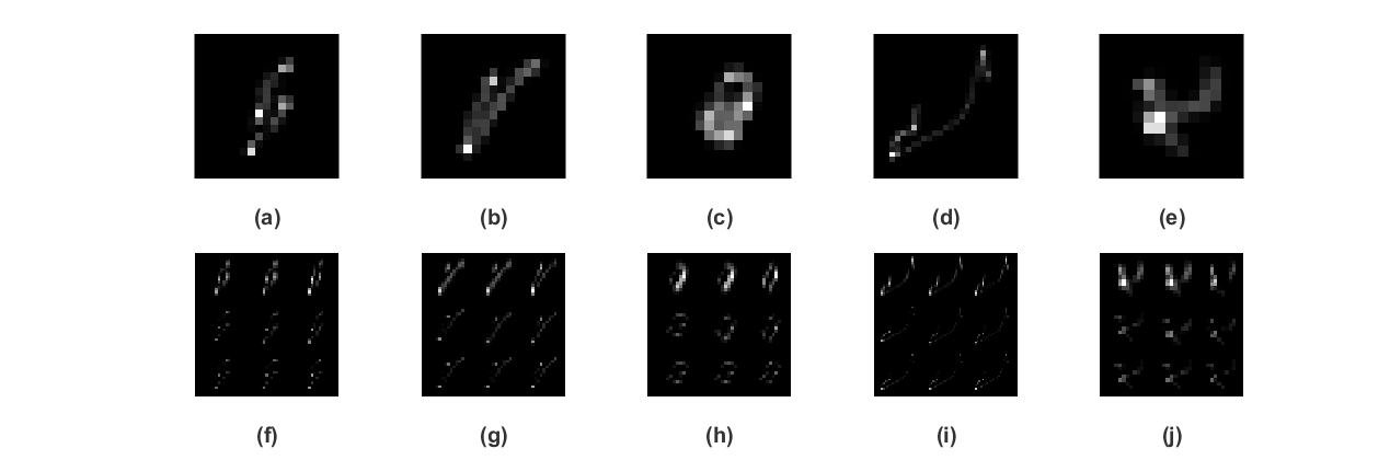
Figure 2: (a-e) Different types of PSF.s from Levin dataset, (f-j) framelet transforms of PSF.s.

2 Motivation and preliminaries

In the following, we explain the details of the proposed model to solve the blind image deblurring problems. Different metrics have been used in different papers to approximate the PSF, and despite having their own advantages, they have some disadvantages. In [18], $\|k\|_{1}$ is used for the PSF, this norm has a good sparse representation, but it causes the creation of a PSF with noise. $\|k\|^{2}_{2}$ is used in [19], despite the advantages of this metric such as convexity and fast speed in calculations and good noise suppression effect, this method creates a dense kernel. Another model that is being used to overcome the disadvantages of previous methods is the use of $\|k\|_{0}$ for example see [20]. In [21] this method is improved by adding a second phrase as $\|\nabla k\|_{0}$ and this change creates a PSF with good sparsity with less noise. Given the structure of the matrix for PSF and considering that most of its elements are zero and it can be considered as a sparse matrix. Using the $l_{0}$ norm is a suitable tool to approximate this matrix that is used in [9]. One way to approximate the $l_{0}$ is to use the $l_{p},~{}p\in(0,1)$ because when $p\rightarrow 0$, $l_{p}\rightarrow l_{0}$. These non-convex metrics are used in [22, 23]. The ratio or difference of $l_{1}$ and $l_{2}$ is another method to approximate the $l_{0}$ that had been studied in various articles [24, 25]. Also $l_{1}-l_{2}$ had been generalized by $l_{1}-\alpha l_{2}$ in [14]. In the present algorithm, $l_{0}-\alpha l_{1}$ metric for $\alpha\in[0,1]$is used instead of the $l_{0}$ metric. Obviously, when $\alpha\rightarrow 0$, $l_{0}-\alpha l_{1}\rightarrow l_{0}$. On the other hand, due to the domain of image pixels that are between zero and one, this metric will always be positive. The graph of this metric is plotted for $[-1,1]\times[-1,1]$ in Fig. 3. As can be seen from the figure, this is a non-convex metric. And that can cause problems in finding a solution. To solve this problem, the proposed model is divided into several new sub-models using the methods that are described. The proposed model, which is introduced, has a suitable behavior in the output in sparsity and less noise. The results of the proposed algorithm are presented at each step, of coarse-to-fine in Fig. 4. The results show, as the size of PSF increases, the number of pixels with zero value increases. In the first iteration, approximately $45\%$ of the pixels are equal to zero and in the last iteration, approximately $14\%$ of the pixels are equal to zero. Then in the early stages of coarse-to-fine method for kernel approximation, it is necessary to reduce the effect of $l_{0}$-norm on the objective function and increase the effect by increasing the iteration. This proposed method is done by reducing the value of a control parameter between the two norms i.e., $\alpha$ in $l_{0}-\alpha l_{1}$. On the other hand, the use of framelet transfer makes the edges of the PSF restored properly. Then the proposed method creates a proper approximations at the early stages of the PSF in coarse-to-fine algorithm. The details of the method are presented in the next section.

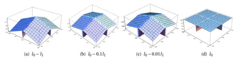
Figure 3: The plot of $l_{0}-\alpha l_{1}$ metric for different values of $\alpha$.

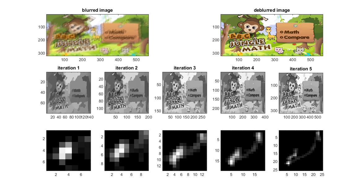
Figure 4: Results of the proposed algorithm in coarse-to-fine steps.

2.1 Framelet transform

One of the fundamental concepts in the signal and image processing is the wavelet theory. In recent years, this discussion has been generalized and used in various articles. The concept of wavelet frames is briefly studied below and reader can find more information about it in [26, 27, 28].

Let $\langle\cdot,\cdot\rangle$ stands for inner product in separable Hilbert space $H$ then a countable set as $X\subseteq H$ is called a tight frame if the following condition holds

$$f=\sum_{\psi\in X}\langle\psi,f\rangle\psi,~{}~{}~{}~{}\forall f\in L^{2}(\mathbb{R}).$$

The wavelet system for a given set as $\Psi=\{\psi_{1},\ldots,\psi_{n}\}$ is defined as the following collection

$$X(\Psi):=\{2^{\frac{j}{2}}\psi_{i}(2^{j}\cdot-k)|1\leq i\leq b;j,k\in\mathbb{Z}\}.$$

Also if $X(\Psi)$ be a tight frame in $H$ then $X(\Psi)$ is named tight wavelet frame and each element of $\Psi$ is named a framelet. In the wavelet theory a compactly supported scaling function as $\phi$ with refinement mask $h_{0}$ that $F\big{(}\phi(2\omega)\big{)}=F(h_{0})F\big{(}\phi(\omega)\big{)}$ is used to construct compactly supported wavelet tight frames. Here $F$ stands the Fourier transform. Also a set of framelets for a given compactly supported scaling function as $\phi$ to construct a wavelet tight frame are defined by

$$F\big{(}\phi(2\omega)\big{)}=F(h_{0})F\big{(}\phi(\omega)\big{)},~{}~{}i=1,\ldots,n,$$

where $F(h_{i}),~{}i=0,\ldots,n$ are considered as $2\pi$-periodic. In the proposed algorithm the piecewise linear B-spline framelets [26] with the refinement mask $F\big{(}h_{0}(\omega)\big{)}=\cos^{2}(\frac{\omega}{2})$ and two framelet masks $F\big{(}h_{1}(\omega)\big{)}=\frac{-\sqrt{2}i}{2}\sin(\omega)$ and $F\big{(}h_{2}(\omega)\big{)}=\sin^{2}(\frac{\omega}{2})$ are used. The corresponding lowpass and highpass filters for these masks are considered as $h_{0}=\frac{1}{4}[1,2,1]$, $h_{1}=\frac{\sqrt{2}}{4}[1,0,-1]$ and $h_{2}=\frac{1}{4}[-1,2,-1]$, respectively. The details of wavelet frame transform can be found in [27, 28]. This transform is used in the next section on the PSF.

2.2 Fractional calculation

Fractional calculation is a concept that has been considered in recent years and has been studied in many different fields of science such as physics, mathematics and computer science. There are different definitions for fractional derivative such as Riemann-Liouville, Caputo, Caputo-Fabrizio and Grünwald-Letnikov (G-L) [15, 29]. As in the use of the ordinary derivative, the discrete form of the derivative is considered for image processing. In the use of the fractional derivative, the discrete form is also efficient. And considering that among the definitions of the fractional derivative, the discrete form of G-L definition is efficient, so this definition is used in image processing [30, 31].

Let $\Omega\subseteq\mathbb{R}^{2}$ be a bounded open set then for a real function $u:\Omega\rightarrow\mathbb{R}^{2}$ the fractional-order gradient is considered as

$$\nabla^{\lambda}u=\big{(}\nabla^{\lambda}_{h}u,\nabla^{\lambda}_{v}u\big{)}^{T},~{}~{}\lambda\in\mathbb{R}^{+}.$$

By using G-L definition, we define

$$\nabla^{\lambda}_{h}u(i,j)=\sum^{L-1}_{l=0}(-1)^{l}C^{l}_{\lambda}u(i-l,j),$$

$$\nabla^{\lambda}_{v}u(i,j)=\sum^{L-1}_{l=0}(-1)^{l}C^{l}_{\lambda}u(i,j-l),$$

where

$$C^{l}_{\lambda}=\frac{\Gamma(\lambda+1)}{\Gamma(l+1)\Gamma(\lambda-l+1)},$$

$\Gamma$ stands for gamma function. This definition is used in the next section to approximate the PSF.

3 Proposed model based on $l_{0}-\alpha l_{1}$ regularization

Details of the proposed model are provided in this section and the numerical algorithms for solving the model are discussed.

3.1 Proposed model

The proposed objective function of the deblurring model is introduced as

$$\arg\min_{k,x}\|x\circledast k-y\|^{2}_{2}+\gamma_{1}P^{\sigma}_{x}+\gamma_{2}P^{\alpha}_{k},$$ (3.1)

where

$$P^{\sigma}_{x}=\sigma\|x\|_{0}+\|\nabla x\|_{0},$$

$$P^{\alpha}_{k}=\|wk\|_{0}-\alpha\|k\|_{1},$$

$\gamma_{1},\gamma_{2}$ and $\sigma$ are the regularization weights and $\alpha\in[0,1]$; $w$ denotes the framelet transform matrix such that $w^{T}w=I$ and $\nabla$ stands for gradient operator where $\nabla x=(\nabla_{h}x,\nabla_{v}x)^{T}$. Also, horizontal and vertical derivatives are obtained using differential filters $\nabla_{h}=[1,-1]$ and $\nabla_{v}=[1,-1]^{T}$. As can be seen from the presented model, the part related to image restoration has not changed with the related papers [9], but the part of the PSF restoration has changed with terms described in the previous parts. This model is non-convex model, therefore, it is necessary to provide a suitable method for solving. The details of finding the answer is introduced in the following subsections.

3.2 Estimating image with blur kernel

To approximate the image from the PSF according to the proposed model, the following model needs to be solved.

$$\arg\min_{x}\|x\circledast k-y\|^{2}_{2}+\gamma_{1}\big{(}\sigma\|x\|_{0}+\|\nabla x\|_{0}\big{)}.$$ (3.2)

The above model is solved in [9], but in the following, a summary of the method described in that paper is given. By using auxiliary variables $a$ and $b=(b_{h},b_{v})$ the problem (3.2) is rewritten as

$$\arg\min_{x,a,b}\|x\circledast k-y\|^{2}_{2}+\beta\|x-a\|^{2}_{2}+\mu_{1}\|\nabla x-b\|^{2}_{2}+\gamma_{1}\big{(}\sigma\|a\|_{0}+\|\nabla b\|_{0}\big{)},$$

where $\beta$ and $\mu_{1}$ are positive constant. Based on the new problem $x$ is obtained by solving

$$\arg\min_{x}\|x\circledast k-y\|^{2}_{2}+\beta\|x-a\|^{2}_{2}+\mu_{1}\|\nabla x-b\|^{2}_{2},$$

which the closed-form solution for this subproblem is given by

$$x=F^{-1}\Big{(}\frac{F^{\ast}(k)F(y)+\beta F(a)+\mu_{1}\sum_{i\in\{v,h\}}F^{\ast}(\nabla_{i})F(b_{i})}{F^{\ast}(k)F(k)+\beta+\mu_{1}\sum_{i\in\{h,v\}}F^{\ast}(\nabla_{i})F(\nabla_{i})}\Big{)},$$ (3.3)

where $\ast$ denotes the complex conjugacy. Also $a$ and $b$ are obtained by following subproblems

$$\arg\min_{a}\beta\|x-u\|^{2}_{2}+\gamma_{1}\sigma\|a\|_{0},$$

$$\arg\min_{b}\mu_{1}\|\nabla x-b\|^{2}_{2}+\gamma_{1}\|b\|_{0}.$$

These subproblems are pixel-wise minimization problem and the solutions are given by [32]

$$a=\left\{\begin{array}[]{l}\begin{array}[]{*{20}{c}}x,&|x|^{2}\geq\frac{\gamma_{1}\sigma}{\beta},\\ \end{array}\\ \begin{array}[]{*{20}{c}}0,&\text{other wise,}\\ \end{array}\\ \end{array}\right.$$ (3.8)

$$b=\left\{\begin{array}[]{l}\begin{array}[]{*{20}{c}}\nabla x,&|\nabla x|^{2}\geq\frac{\gamma_{1}}{\mu_{1}},\\ \end{array}\\ \begin{array}[]{*{20}{c}}0,&\text{other wise.}\\ \end{array}\\ \end{array}\right.$$ (3.13)

A summary of the described method is given in Algorithm 1.

Input: Blurred image $y$ and blur kernel $k$.

$x\leftarrow y$, $\beta\leftarrow 2\gamma_{1}\sigma$.

repeat

     obtain $a$ by (3.8).

     $\mu_{1}\leftarrow 2\gamma_{1}$.

     repeat

         obtain $b$ by (3.13).

         obtain $x$ by (3.3).

         $\mu_{1}\leftarrow 2\mu_{1}$.

     until $\mu_{1}>\mu^{max}$

     $\beta\leftarrow 2\beta$.

until $\beta>\beta^{\max}$

Output: Intermediate latent image $x$.

3.3 Estimating PSF with image

In order to approximate the PSF in model (3.1), it is necessary to solve the following problem

$$\arg\min_{k}\|x\circledast k-y\|^{2}_{2}+\gamma_{2}\big{(}\|wk\|_{0}-\alpha\|k\|_{1}\big{)}.$$ (3.14)

Solving the above problem directly by using the intermediate latent image does not give a good output and in [7] recommends using the gradient operator to solve the above problem. Then based on the gradient operator, the following problem is proposed for (3.14).

$$\arg\min_{k}\|\nabla x\circledast k-\nabla y\|^{2}_{2}+\gamma_{2}\big{(}\|wk\|_{0}-\alpha\|k\|_{1}\big{)}.$$

But in the following, a general model based on the fraction gradient operator is presented to solve the problem (3.14) as

$$\arg\min_{k}\|\nabla^{\lambda}x\circledast k-\nabla^{\lambda}y\|^{2}_{2}+\gamma_{2}\big{(}\|wk\|_{0}-\alpha\|k\|_{1}\big{)}.$$

Specifically, when $\lambda$ is equal to $1$, the ordinary model by gradient operator is obtained. By introducing auxiliary variables $c$ and $d$ for $wk$ and $k$, respectively, we get

$$\arg\min_{k,c}\|\nabla^{\lambda}x\circledast k-\nabla^{\lambda}y\|^{2}_{2}+\gamma_{2}\big{(}\|c\|_{0}-\alpha\|d\|_{1}\big{)},$$

$$\text{s.t.}~{}c=wk,~{}d=k$$

The augmented form for the above problem can be get as

$$\arg\min_{k,c}\|\nabla^{\lambda}x\circledast k-\nabla^{\lambda}y\|^{2}_{2}+\gamma_{2}\|c\|_{0}+\mu_{2}\|wk-c\|^{2}_{2}-\gamma_{2}\alpha\|d\|_{1}+\mu_{3}\|d-k\|^{2}_{2}.$$ (3.15)

To solve the above problem, in the first step, the solution of $c$ is studied. By (3.15), the subproblem for $c$ can be written as

$$\arg\min_{c}\gamma_{2}\|c\|_{0}+\mu_{2}\|wk-c\|_{2}.$$

As discussed in the previous section, this problem is pixel-wise minimization problem and the solution is obtained as

$$c=\left\{\begin{array}[]{l}\begin{array}[]{*{20}{c}}wk,&|wk|^{2}\geq\frac{\gamma_{2}}{\mu_{2}},\\ \end{array}\\ \begin{array}[]{*{20}{c}}0,&\text{other wise}.\\ \end{array}\\ \end{array}\right.$$ (3.20)

In the next step, we approximate the value of $k$. For this purpose by using $\eqref{Es22}$, the following subproblem is obtained

$$\arg\min_{k}\|\nabla^{\lambda}x\circledast k-\nabla^{\lambda}y\|^{2}_{2}+\mu_{2}\|wk-c\|^{2}_{2}+\mu_{3}\|k-d\|^{2}_{2}.$$ (3.21)

By using the optimal condition for (3.21) and fast Fourier transform, the closed-form of the final solution for $k$ is written as

$$k=F^{-1}\Big{(}\frac{\sum_{i\in\{h,v\}}F^{\ast}(\nabla^{\lambda}_{i}x)F(\nabla^{\lambda}_{i}y)+\mu_{3}F(d)+\mu_{2}F(w^{\ast}c)}{\sum_{i\in\{h,v\}}F^{\ast}(\nabla^{\lambda}_{i}x)F(\nabla^{\lambda}_{i}x)+\mu_{3}+\mu_{2}}\Big{)}.$$ (3.22)

Now, the next subproblem that is needed to find $d$ is studied. This subproblem is written as

$$\arg\min_{d}-\gamma_{2}\alpha\|d\|_{1}+\mu_{3}\|k-d\|^{2}_{2}.$$

Similar to split Bregman iteration method [33, 34], the following iterative method is proposed to solve this problem

$$d^{n+1}=\arg\min_{d}-\gamma_{2}\alpha\|d\|_{1}+\mu_{3}\|d-k-b^{n}\|^{2}_{2},$$ (3.23)

$$b^{n+1}=b^{n}+(k-d^{n+1}).$$ (3.24)

The solution of problem (3.23) with condition $|-\frac{\gamma_{2}\alpha}{\mu_{3}}|<1$ is obtained by using the proximal mapping for $l_{1}$-norm as [35]

$$d^{n+1}=k+b^{n}.$$ (3.25)

The above processing can be expressed in the following algorithm. According to the structure of Algorithm 2, the value of $|-\frac{\gamma_{2}\alpha}{\mu_{3}}|$ is always lower than one, therefore, a local minimum value can be found for (3.23).

Input: Blurred image $y$ and Intermediate latent image $x$.

$b=0,k=0$, $\mu_{2}\leftarrow 2\gamma_{2}$.

repeat

     obtain $c$ by (3.20).

     $\mu_{3}\leftarrow 2\mu_{2}$.

     repeat

         obtain $d$ by (3.25).

         $b\leftarrow b+k-d$.

         obtain $k$ by (3.22).

         $\mu_{3}\leftarrow 2\mu_{3}$

     until $\mu_{3}>\mu_{3}^{max}$

     $\mu_{2}\leftarrow 2\mu_{2}$.

until $\mu_{2}>\mu_{2}^{\max}$

Output: Intermediate kernel $k$.

3.4 Coarse-to-fine framework for PSF

In the previous subsections, the methods of image restoring by the PSF and PSF restoring by the image are studied. Using the above methods directly to restore image information does not always work. One of the most effective methods that is considered in various algorithms is the use of an image pyramid framework in a coarse-to-fine method [7]. Due to the fact that sharp edges is effective in approximating the PSF, so using the fraction gradient operator improves the kernel. This algorithm is given in Algorithm 3. According to the structure of the proposed algorithm, it is observed that by increasing the number of iterations and approaching the actual size of the image, the constant $\alpha$ decreases to increase the effect of the $l_{0}$ norm. In the last step, to increase the quality of the restored image, depending on the type of image, a non-blind image deblurring algorithm based on the obtained PSF is used. Also to reduce ringing artifacts, simple but efficient method based on Fourier domain restoration filter and extrapolated image that is introduced in [36] is used in the proposed algorithm. Also in this algorithm the proposed method for threshold of truncating gradients in [7] is used to estimate kernel with this difference that fractional gradient values are used instead of the ordinary gradient values. Numerical results related to the proposed algorithms are studied in the next section.

Input: Blurred image $y$, the size of PSF, $\lambda$.

Obtain $k$ by the coarser level method.

for $i=1\rightarrow 5$ do

     Obtain $x$ by Algorithm 1.

     Obtain $k$ by Algorithm 2.

     $\gamma_{1}\leftarrow\max\{\gamma_{1}/1.1,10e-4\}$.

     $\alpha\leftarrow\max\{\alpha/1.1,10e-4\}$.

end for

Output: $k$ and intermediate image $x$.

4 Experiment results

In order to evaluate the performance of the proposed algorithm, different types of images as text, face, natural and low-light images are studied in this section. Also Windows 10-64bit, Intel(R) Core(TM) i3-5005U CPU @2.00GHz, by matlab 2014b have been used for the calculations. The results of the algorithm are evaluated using different tests such as Information content Weighted Structural Similarity Measure (IW-SSIM)[38], Multi-scale Structural Similarity (M-SSIM) [39], Feature Structural Similarity(F-SSIM) [40] and Peak Signal-to-Noise Ratio (PSNR).

Levin dataset: As a first example, we use Levin dataset. The results are given in Table 1. In this table the first number in parentheses stands for number of image and the second number denotes the number of kernel in dataset. The results in this table are compared with the results in [9, 37], and although in some cases the results of the proposed method have lower values compared to these methods, but in general the average of the proposed method has a better output compared to these methods.

Table 1: Results for Levin dataset.

	method in [9]				method in [37]				proposed method
(imgae,kernel)	PSNR	IW-SSIM	M-SSIM	F-SSIM	PSNR	IW-SSIM	M-SSIM	F-SSIM	PSNR	IW-SSIM	M-SSIM	F-SSIM
(1,1)	33.9744	0.9440	0.9649	0.8857	33.3213	0.9213	0.9509	0.8584	34.0847	0.9464	0.9672	0.8839
(1,2)	31.8732	0.6811	0.8168	0.7585	31.8640	0.7404	0.8463	0.7733	31.9585	0.7452	0.8502	0.7699
(1,3)	32.8360	0.8487	0.9114	0.8291	32.4375	0.8054	0.8861	0.8122	33.1591	0.8830	0.9307	0.8464
(1,4)	31.1792	0.8943	0.9170	0.8265	31.5524	0.9119	0.9281	0.8460	30.8961	0.8587	0.8988	0.7998
(1,5)	34.2503	0.9451	0.9657	0.8893	36.4330	0.9820	0.9883	0.9431	34.4087	0.9423	0.9633	0.8773
(1,6)	31.8843	0.7944	0.8760	0.8031	32.3136	0.8351	0.8998	0.8198	32.3843	0.8733	0.9202	0.8370
(1,7)	34.2585	0.9600	0.9699	0.9039	35.3590	0.9764	0.9806	0.9296	34.6986	0.9706	0.9756	0.9171
(1,8)	31.0571	0.8902	0.9228	0.8379	32.0271	0.9335	0.9527	0.8755	31.2542	0.9268	0.9422	0.8708
mean	32.6641	0.8697	0.9181	0.8417	33.1635	0.8882	0.9291	0.8573	32.8555	0.8933	0.9310	0.8503
(2,1)	31.2466	0.7454	0.8206	0.7363	31.6891	0.8299	0.8750	0.7803	32.5778	0.9146	0.9356	0.8461
(2,2)	30.3489	0.4617	0.6317	0.6892	30.2430	0.4208	0.6092	0.6903	30.4562	0.4872	0.6551	0.7005
(2,3)	30.3637	0.4632	0.6443	0.6777	30.3370	0.4444	0.6414	0.6800	30.4052	0.4767	0.6577	0.6815
(2,4)	30.7992	0.8816	0.8988	0.8118	30.8806	0.8492	0.8802	0.7938	30.6572	0.8694	0.8887	0.8021
(2,5)	32.9145	0.9093	0.9328	0.8485	32.2432	0.8434	0.8850	0.8124	32.9566	0.9140	0.9357	0.8538
(2,6)	31.2432	0.7884	0.8388	0.7592	32.3850	0.9035	0.9225	0.8306	31.6021	0.8193	0.8757	0.7596
(2,7)	31.3156	0.8057	0.8603	0.7645	31.1319	0.7828	0.8440	0.7683	31.8457	0.8620	0.8996	0.8009
(2,8)	31.3195	0.9265	0.9392	0.8596	31.4929	0.8911	0.9173	0.8279	31.4341	0.9289	0.9415	0.8595
mean	31.1939	0.7477	0.8322	0.7683	31.3003	0.7456	0.8218	0.7730	31.4919	0.7840	0.8487	0.7880
(3,1)	32.8699	0.9063	0.9376	0.8265	33.6145	0.9438	0.9619	0.8638	33.8982	0.9544	0.9690	0.8841
(3,2)	31.3196	0.6660	0.7868	0.7026	31.4307	0.6967	0.8030	0.7102	31.7872	0.7918	0.8621	0.7515
(3,3)	31.5949	0.7848	0.8587	0.7376	31.6511	0.7705	0.8505	0.7297	31.8953	0.8285	0.8881	0.7787
(3,4)	31.3626	0.8627	0.9000	0.7941	31.9126	0.8965	0.9235	0.8216	31.5777	0.8844	0.9156	0.8117
(3,5)	34.2074	0.9522	0.9680	0.8779	35.6246	0.9801	0.9864	0.9250	35.5800	0.9782	0.9852	0.9235
(3,6)	31.7835	0.7928	0.8621	0.7455	31.7473	0.7544	0.8400	0.7259	31.6417	0.7841	0.8619	0.7573
(3,7)	33.7404	0.9534	0.9665	0.8812	36.3052	0.9863	0.9888	0.9440	34.6544	0.9745	0.9803	0.9197
(3,8)	31.5923	0.9412	0.9553	0.8683	31.2153	0.8531	0.8973	0.7831	31.4176	0.9235	0.9437	0.8461
mean	32.3088	0.8574	0.9082	0.8042	32.9377	0.8602	0.9064	0.8129	32.8065	0.8899	0.9257	0.8341
(4,1)	34.7037	0.9565	0.9735	0.9142	35.8420	0.9675	0.9809	0.9269	34.6905	0.9546	0.9728	0.9157
(4,2)	30.2999	0.5933	0.7463	0.7456	30.5067	0.5926	0.7552	0.7516	30.6186	0.6653	0.7894	0.7717
(4,3)	30.6522	0.6810	0.8011	0.7630	31.0039	0.7400	0.8366	0.7896	31.4443	0.78910	0.8700	0.8051
(4,4)	29.0565	0.6153	0.6948	0.7039	30.9436	0.8079	0.8675	0.8029	31.3079	0.8121	0.8773	0.8083
(4,5)	31.3412	0.7375	0.8289	0.7816	31.1517	0.6593	0.7867	0.7654	32.5577	0.8529	0.9089	0.8328
(4,6)	31.8929	0.8596	0.9093	0.8392	32.6546	0.8786	0.9207	0.8539	33.7876	0.9456	0.9644	0.9029
(4,7)	31.0731	0.8548	0.8979	0.8193	32.5106	0.8684	0.9120	0.8425	32.7110	0.9075	0.9374	0.8645
(4,8)	30.0096	0.8313	0.8769	0.8124	31.8375	0.9026	0.9345	0.8730	31.5005	0.9229	0.9465	0.8836
mean	31.1286	0.7662	0.8411	0.7974	32.0563	0.8021	0.8743	0.8257	32.3273	0.8563	0.9083	0.8481
mean	31.8239	0.8103	0.8711	0.8029	32.3644	0.8240	0.8829	0.8172	32.3703	0.8559	0.9034	0.8301

Text image: Images containing text usually appear in images obtained by scanning a text. In recent years, with the expansion of the use of smart phones, scanning software has expanded [41]. Various factors can affect the quality of the output image, such as hand shake when using scanning software by smart phone. The results for two text images such that blurred by kernel 01 and 04 in Levin dataset are shown in Fig.s 5-7. The results of the proposed method are compared with [7, 9, 37, 42, 44]. In Fig. 5, the results for MS-SSIM, IW-SSIM and F-SSIM are given. Also Fig. 6 shows output deblurred images. The Fig. 6 shows the close approximation of the PSF by the proposed algorithm. Also realistic blurred text image includes car license plate is restored by the proposed algorithm and compared by methods in [37, 44, 45] in Fig 7. As can be seen from these figures, the proposed algorithm has a better output compared to the other methods.

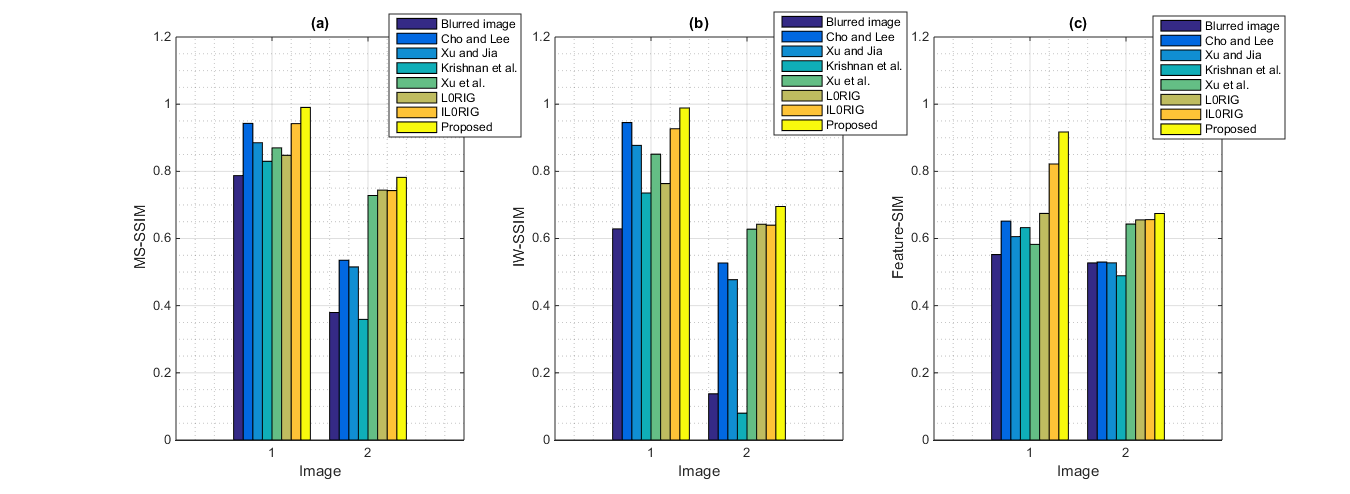
Figure 5: Compare the results for IW-SSIM, M-SSIM and F-SSIM.

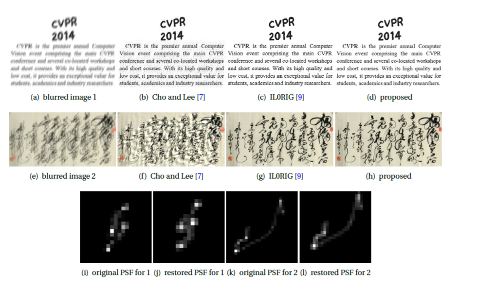
Figure 6: Visual comparison for text images deblurring.

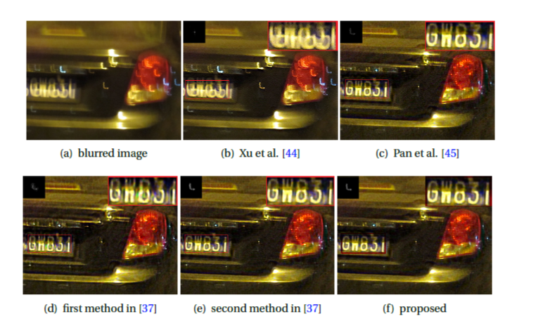
Figure 7: Visual comparison for realistic blurred text image.

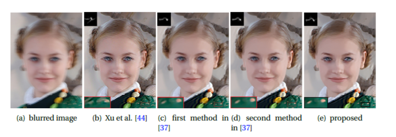
Figure 8: Visual comparison for realistic blurred face image.

Face image: Another image that is considered in computer science is the face image. This type of image is used in face recognition in topics related to artificial intelligence, so increasing the image quality of the face before use can be considered. Numerical results related to the proposed method are given in Fig.s 8-9 and are compared with some methods. The results show the efficiency of the proposed algorithm for face images. The results show that proposed algorithm compares favorably or even better against compared methods. It is also seen in Fig. 9 that increasing the kernel size in the algorithm, unlike the compared methods, has little effect on the quality of the restored image.

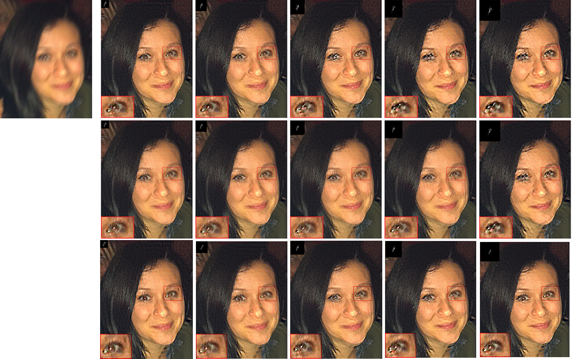
Figure 9: Restored face image with the used kernel sizes $\{25,35,45,55,65\}$, from left to right, respectively. First row, method in [45]; second row, method in [37]; third row, proposed method.

Natural image: Three real natural images are studied in this example. The results are given and compared with method in [37, 44, 45] in Fig.s 10 and 11. The results for this type of images show the efficiency of the proposed algorithm in restoring blurred nature images.

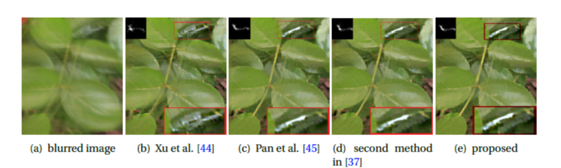
Figure 10: Visual comparison for realistic blurred nature image.

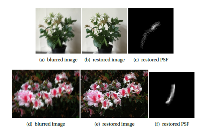
Figure 11: Obtained results by the proposed method for two nature image.

Low-light image: Restoring the low-light image is difficult due to their structure and requires the design of a special algorithm for this type of image [46, 48]. However, according to the results of the proposed method in Fig. 12, the results show that the proposed algorithm is efficient in recycling this type of images. In this comparison, we note that the algorithm in [46] is designed specifically for this type of problems.

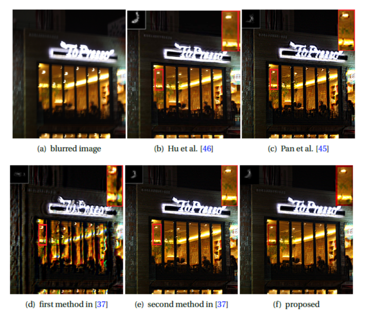
Figure 12: Visual comparison for realistic blurred low-light image.

Camera motion: As a final example in this section we review a few examples of real camera motion dataset in [47] . The results for this dataset are given in Fig.s 13 and 14. The results of F-SSIM and PSNR values for the church image in this dataset are given in Fig. 13 and compared with methods in [7, 8, 43, 44, 49, 50, 51]. In this diagram, the restored images of proposed and other methods are compared with around 200 ground truth images and the best result is reported as the main results. Also the restored images of the clock image with kernel 8 for the proposed and other algorithms are shown in Fig. 14.

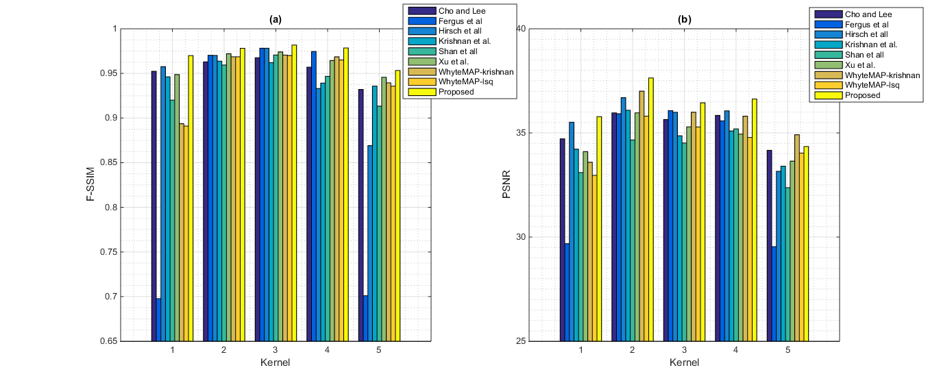
Figure 13: Compare the results for F-SSIM and PSNR with the kernels 1,2,3 and 4.

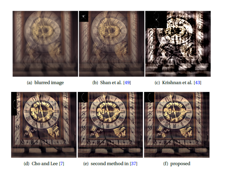
Figure 14: Deblurring results of image 1 with kernel 8 in dataset [47].

5 Conclusion

In this paper, the difference between two norms zero and one is used to approximate the point spread function in blind image deblurring problems. Also in the proposed algorithm, two concepts of framelet and fractional calculations have been used. The proposed algorithm is evaluated on different types of images with different PSF sizes. The results are compared with the other methods and the outputs show the efficiency of the proposed algorithm in deblurring performance.

References

- [1] Hansen, Per Christian, James G. Nagy, and Dianne P. O’leary. Deblurring images: matrices, spectra, and filtering. Society for Industrial and Applied Mathematics, 2006.
- [2] Christiansen, M. and Hanke, M., 2008. Deblurring methods using antireflective boundary conditions. SIAM Journal on Scientific Computing, 30(2), pp.855-872.
- [3] Campisi, Patrizio, and Karen Egiazarian, eds. Blind image deconvolution: theory and applications. CRC press, 2017.
- [4] Liu, Gang, Ting-Zhu Huang, Jun Liu, and Xiao-Guang Lv. "Total variation with overlapping group sparsity for image deblurring under impulse noise." PloS one 10, no. 4 (2015): e0122562.
- [5] Parvaz, Reza. "Color image restoration with impulse noise based on fractional-order total variation and framelet." arXiv preprint arXiv:2110.15170 (2021).
- [6] Rajagopalan, A. N., and Rama Chellappa, eds. Motion deblurring: Algorithms and systems. Cambridge University Press, 2014.
- [7] Cho, Sunghyun, and Seungyong Lee. "Fast motion deblurring." In ACM SIGGRAPH Asia 2009 papers, pp. 1-8. 2009.
- [8] Whyte, Oliver, Josef Sivic, and Andrew Zisserman. "Deblurring shaken and partially saturated images." International journal of computer vision 110, no. 2 (2014): 185-201.
- [9] Pan, Jinshan, Zhe Hu, Zhixun Su, and Ming-Hsuan Yang. "-regularized intensity and gradient prior for deblurring text images and beyond." IEEE transactions on pattern analysis and machine intelligence 39, no. 2 (2016): 342-355.
- [10] Cai, Jian-Feng, Stanley Osher, and Zuowei Shen. "Linearized Bregman iterations for frame-based image deblurring." SIAM Journal on Imaging Sciences 2, no. 1 (2009): 226-252.
- [11] Liu, Jingjing, Yifei Lou, Guoxi Ni, and Tieyong Zeng. "An image sharpening operator combined with framelet for image deblurring." Inverse Problems 36, no. 4 (2020): 045015.
- [12] Levin, Anat, Yair Weiss, Fredo Durand, and William T. Freeman. "Understanding and evaluating blind deconvolution algorithms." In 2009 IEEE Conference on Computer Vision and Pattern Recognition, pp. 1964-1971. IEEE, 2009.
- [13] Liu, Jingjing, Anqi Ni, and Guoxi Ni. "A nonconvex model for image restoration with impulse noise." Journal of Computational and Applied Mathematics 378 (2020): 112934.
- [14] Lou, Yifei, and Ming Yan. "Fast minimization via a proximal operator." Journal of Scientific Computing 74, no. 2 (2018): 767-785.
- [15] Yang, Xiao-Jun. General fractional derivatives: theory, methods and applications. CRC Press, 2019.
- [16] Guo, Lin, Xi-Le Zhao, Xian-Ming Gu, Yong-Liang Zhao, Yu-Bang Zheng, and Ting-Zhu Huang. "Three-dimensional fractional total variation regularized tensor optimized model for image deblurring." Applied Mathematics and Computation 404 (2021): 126224.
- [17] Fairag, Faisal, Adel Al-Mahdi, and Shahbaz Ahmad. "Two-Level method for the total fractional-order variation model in image deblurring problem." Numerical Algorithms 85, no. 3 (2020): 931-950.
- [18] Shan, Qi, Jiaya Jia, and Aseem Agarwala. "High-quality motion deblurring from a single image." Acm transactions on graphics (tog) 27, no. 3 (2008): 1-10.
- [19] Pan, Jinshan, Zhe Hu, Zhixun Su, and Ming-Hsuan Yang. "Deblurring text images via L0-regularized intensity and gradient prior." In Proceedings of the IEEE Conference on Computer Vision and Pattern Recognition, pp. 2901-2908. 2014.
- [20] Li, Jie, and Wei Lu. "Blind image motion deblurring with L0-regularized priors." Journal of Visual Communication and Image Representation 40 (2016): 14-23.
- [21] Zhang, Fengjun, Wei Lu, Hongmei Liu, and Fei Xue. "Natural image deblurring based on -regularization and kernel shape optimization." Multimedia tools and applications 77, no. 20 (2018): 26239-26257.
- [22] Zhao, Chenping, Yingjun Wang, Hongwei Jiao, Jingben Yin, and Xuezhi Li. "-Norm-Based Sparse Regularization Model for License Plate Deblurring." IEEE Access 8 (2020): 22072-22081.
- [23] Estatico, Claudio, Serge Gratton, Flavia Lenti, and David Titley-Peloquin. "A conjugate gradient like method for p-norm minimization in functional spaces." Numerische Mathematik 137, no. 4 (2017): 895-922.
- [24] Repetti, Audrey, Mai Quyen Pham, Laurent Duval, Emilie Chouzenoux, and Jean-Christophe Pesquet. "Euclid in a Taxicab: Sparse Blind Deconvolution with Smoothed Regularization." IEEE signal processing letters 22, no. 5 (2014): 539-543.
- [25] Lou, Yifei, Stanley Osher, and Jack Xin. "Computational aspects of constrained minimization for compressive sensing." In Modelling, computation and optimization in information systems and management sciences, pp. 169-180. Springer, Cham, 2015.
- [26] Ron, Amos, and Zuowei Shen. "Affine systems in : the analysis of the analysis operator." Journal of Functional Analysis 148, no. 2 (1997): 408-447.
- [27] Chai, Anwei, and Zuowei Shen. "Deconvolution: A wavelet frame approach." Numerische Mathematik 106, no. 4 (2007): 529-587.
- [28] Daubechies, Ingrid, Bin Han, Amos Ron, and Zuowei Shen. "Framelets: MRA-based constructions of wavelet frames." Applied and computational harmonic analysis 14, no. 1 (2003): 1-46.
- [29] Mainardi, Francesco. "Fractional calculus: theory and applications." (2018): 145.
- [30] Cafagna, Donato. "Fractional calculus: A mathematical tool from the past for present engineers [Past and present]." IEEE Industrial Electronics Magazine 1, no. 2 (2007): 35-40.
- [31] Sridevi, G., and S. Srinivas Kumar. "Image inpainting based on fractional-order nonlinear diffusion for image reconstruction." Circuits, Systems, and Signal Processing 38, no. 8 (2019): 3802-3817.
- [32] Xu, Li, Cewu Lu, Yi Xu, and Jiaya Jia. "Image smoothing via L 0 gradient minimization." In Proceedings of the 2011 SIGGRAPH Asia conference, pp. 1-12. 2011.
- [33] Cai, Jian-Feng, Stanley Osher, and Zuowei Shen. "Split Bregman methods and frame based image restoration." Multiscale modeling simulation 8, no. 2 (2010): 337-369.
- [34] Goldstein, Tom, and Stanley Osher. "The split Bregman method for L1-regularized problems." SIAM journal on imaging sciences 2, no. 2 (2009): 323-343.
- [35] Beck, Amir. First-order methods in optimization. Society for Industrial and Applied Mathematics, 2017.
- [36] Liu, Renting, and Jiaya Jia. "Reducing boundary artifacts in image deconvolution." In 2008 15th IEEE International Conference on Image Processing, pp. 505-508. IEEE, 2008.
- [37] Wen, Fei, Rendong Ying, Yipeng Liu, Peilin Liu, and Trieu-Kien Truong. "A simple local minimal intensity prior and an improved algorithm for blind image deblurring." IEEE Transactions on Circuits and Systems for Video Technology (2020).
- [38] Wang, Zhou, and Qiang Li. "Information content weighting for perceptual image quality assessment." IEEE Transactions on image processing 20, no. 5 (2010): 1185-1198.
- [39] Wang, Zhou, Eero P. Simoncelli, and Alan C. Bovik. "Multiscale structural similarity for image quality assessment." In The Thrity-Seventh Asilomar Conference on Signals, Systems Computers, 2003, vol. 2, pp. 1398-1402. Ieee, 2003.
- [40] Zhang, Lin, Lei Zhang, Xuanqin Mou, and David Zhang. "FSIM: A feature similarity index for image quality assessment." IEEE transactions on Image Processing 20, no. 8 (2011): 2378-2386.
- [41] Völcker, Athénaïs. "The influence of scanning mobile apps on consumer behavior regarding cosmetic products." Master’s thesis, Handelshøyskolen BI, 2021.
- [42] Xu, Li, and Jiaya Jia. "Two-phase kernel estimation for robust motion deblurring." In European conference on computer vision, pp. 157-170. Springer, Berlin, Heidelberg, 2010.
- [43] Krishnan, Dilip, Terence Tay, and Rob Fergus. "Blind deconvolution using a normalized sparsity measure." In CVPR 2011, pp. 233-240. IEEE, 2011.
- [44] Xu, Li, Shicheng Zheng, and Jiaya Jia. "Unnatural l0 sparse representation for natural image deblurring." In Proceedings of the IEEE conference on computer vision and pattern recognition, pp. 1107-1114. 2013.
- [45] Pan, Jinshan, Deqing Sun, Hanspeter Pfister, and Ming-Hsuan Yang. "Blind image deblurring using dark channel prior." In Proceedings of the IEEE Conference on Computer Vision and Pattern Recognition, pp. 1628-1636. 2016.
- [46] Hu, Zhe, Sunghyun Cho, Jue Wang, and Ming-Hsuan Yang. "Deblurring low-light images with light streaks." In Proceedings of the IEEE Conference on Computer Vision and Pattern Recognition, pp. 3382-3389. 2014.
- [47] Köhler, Rolf, Michael Hirsch, Betty Mohler, Bernhard Schölkopf, and Stefan Harmeling. "Recording and playback of camera shake: Benchmarking blind deconvolution with a real-world database." In European conference on computer vision, pp. 27-40. Springer, Berlin, Heidelberg, 2012.
- [48] Zhou, Chu, Minggui Teng, Jin Han, Chao Xu, and Boxin Shi. "DeLiEve-Net: Deblurring Low-light Images with Light Streaks and Local Events." In Proceedings of the IEEE/CVF International Conference on Computer Vision, pp. 1155-1164. 2021.
- [49] Shan, Qi, Jiaya Jia, and Aseem Agarwala. "High-quality motion deblurring from a single image." Acm transactions on graphics (tog) 27, no. 3 (2008): 1-10.
- [50] Hirsch, Michael, Christian J. Schuler, Stefan Harmeling, and Bernhard Schölkopf. "Fast removal of non-uniform camera shake." In 2011 International Conference on Computer Vision, pp. 463-470. IEEE, 2011.
- [51] Fergus, Rob, Barun Singh, Aaron Hertzmann, Sam T. Roweis, and William T. Freeman. "Removing camera shake from a single photograph." In ACM SIGGRAPH 2006 Papers, pp. 787-794. 2006.