Basin sizes depend on stable eigenvalues in the Kuramoto model

Abstract

We show that for the Kuramoto model (with identical phase oscillators equally coupled) its global statistics and size of the basins of attraction can be estimated through the eigenvalues of all stable (frequency) synchronized states. This result is somehow unexpected since, by doing that, one could just use local analysis to obtain global dynamic properties. But recent works based on Koopman and Perron-Frobenius operators demonstrate that global features of a nonlinear dynamical system, with some specific conditions, are somehow encoded in the local eigenvalues of its equilibrium states. Recognized numerical simulations in the literature reinforce our analytical results.

Introduction

Since the pioneering studies of Winfree on biological rhythms in the end of 60’s Winfree1967 , phase oscillators have been playing a central role in the study of collective behavior. The most famous derivation, the Kuramoto model Kuramoto1975 ; Kuramoto1984 and its variants, has been successfully employed to understand problems related to synchronization in various areas of science. It includes synchronization in flashing fireflies Ermentrout1991 , circadian rhythms Antonsen2008 , swarming dynamics Keeffe2017 , cardiac pacemaker cells Osaka2017 , superconducting Josephson junctions Wiesenfeld1998 , power-grid networks Dorfler2013 , and the Millenium bridge oscillation Strogatz2005 . In front of this vast diversity of these dynamical systems, emerges a relevant question that guides this paper: what are the conditions that lead each system to the correct operation?

Basin of attraction, the set of initial conditions from which the solutions converge asymptotically to a given attractor, is an intricate and fundamental concept in dynamics. Although the definition is straightforward, the boundaries of the basin as well as its measure, may be difficult to study even in low-dimensional systems and also for such simple attractors as stable equilibrium states. Since the basin can include the points quite distant from the attracting set, the size of the basin, as a general rule, is not determined by the local properties of the attractor. In dissipative maps and flows, it is delimited by the complex geometrical configuration of stable manifolds of unstable invariant sets, which may imply in fractal boundaries Ott2002 . This feature makes statistics a proper method to evaluate quantities in a basin of attraction. That approach has been applied in the Kuramoto model of coupled phase oscillators, in the context of stable synchronized twisted states Wiley2006 ; Delabays2017 ; Ochab2010 . These studies focused on the size of the basin, lately interpreted in networks as the basin stability: the likelihood quantification of returning to the same synchronized state Menck2013 .

In particular, in 2006 Wiley, Strogatz, and Girvan Wiley2006 investigated the Kuramoto model of $N$ identical phase oscillators on a ring, each one equally coupled with the $R$ nearest neighbors on either side [Eq. (1)]. The authors studied, through numerical experiments and also analytically, for different low values of $R$ some relevant aspects of the so-called sync basin (the attraction basin of the state of full synchronization for which, in the appropriate co-rotating reference frame, all oscillators share the steady phase value). They showed that for $R/N>0.34$, the sync basin is the whole phase space, except for a set of measure zero. Below this critical value the stable steady configurations called $q$-twisted states, characterized by a constant difference of phases between the neighboring units, emerge in the phase space. The number of twists $q$ counts overall rotations around the circle that occur while passing along the ensemble from the first to the last unit. The simulations revealed that (i) the probability of the final twisted state having $q$ twists follows a Gaussian distribution $\sim\exp[-q^{2}/(2\sigma^{2})]$ with respect to the winding number $q$, and (ii) the standard deviation $\sigma$ of this distribution scales as $\sqrt{N/R}$, namely $\sigma\sim 0.2\,\sqrt{N/R}$. Remarkably, this finding was supported by a heuristic argument for such statistical patterns, leaving rigorous derivations of (i) and (ii) as open questions.

For the next-neighbor coupling ($R=1$), this problem was revisited in Delabays2017 with an accurate numerical method to measure the volume of the basin for each stable state. The authors obtained a typical linear size [$\alpha_{\tau}(q)$] for each basin of attraction of $q$-twisted stable state, so that the volume of the basin of attraction of each stable state is proportional to $V_{q}\sim\alpha_{\tau}^{N}(q)$. Besides these studies another important step in the knowledge of the basin of attraction of the Kuramoto model, still locally coupled, was given by Ochab and Góra Ochab2010 . They observed a direct correlation between the size of basins of attraction and the respective eigenvalues of the Jacobian matrices of stable $q$-twisted states: solutions having the maximal negative eigenvalue closer to zero (less stable) feature smaller basins of attraction than the more stable solutions for which all eigenvalues are strongly negative. In general one does not expect that local properties of equilibrium states have direct relations with global properties of the state space, but that result is consistent with recent mathematical results about global properties of certain nonlinear systems on compact manifolds which shall be discussed further and will also serve as basis for the study that we present here. Keeping in mind that in the Kuramoto model the only dynamic action is the attractive or repulsive interaction between the nodes, and that the most attractive configuration possesses the largest size basin of attraction, we delve into this idea and suggest a theoretical description for the size of the basin of attraction in the Kuramoto model.

Following we start with a brief summary of the Kuramoto model and of recent mathematical results concerning global and local properties of certain nonlinear systems on compact manifolds. Using some approximations, we obtain an analytical expression that has many similarities with the basin volume distribution obtained by Wiley2006 , mentioned above. Then our analytical results are compared with the numerical experiments strengthening the evidence for the strong correlation between eigenvalues and basin sizes and providing more arguments towards an explanation of open questions (i) and (ii). Our approach should work with systems that can be reduced to the Kuramoto model, as done recently in an experimental network of nanoelectromechanical oscillators Matheny2019 , but we expect that our approach can be applied to other systems, as discussed in Final Remarks.

I Theoretical aspects

Kuramoto model: solutions and eigenvalues

Following Wiley2006 , we consider here a system of $N$ identical Kuramoto oscillators on a regular ring where each oscillator is coupled with equal strength to its $R$ nearest neighbors on either side. In the co-rotating reference frame the time evolution of this system is governed by the following set of ODEs

$$\dot{\theta_{j}}=\sum_{k=j-R}^{j+R}G\,\sin(\theta_{k}-\theta_{j})\,,\,\,j=1,2,...,N;$$ (1)

where the index $k$ is periodic mod $N$, the coupling constant $G$ is positive and can be completely removed from the equations by rescaling the time.

As pointed out in Wiley2006 , the set of equations (1) is a gradient system that can be recast as $\dot{\theta}=-\nabla V$ with e.g. $V(\theta_{1},\ldots,\theta_{N})=G\sum_{i,j}\cos(\theta_{i}-\theta_{j})$ so that $V$ is bounded both from below and from above: $-N^{2}G\leq V\leq N^{2}G$. Therefore $dV/dt=-(\nabla V)^{2}$ and all trajectories, except the points of equilibrium and their stable manifolds, are flowing “monotonically downhill” and asymptotically tend to those of the equilibria that correspond to the local minima of $V$. For this reason, “we need not concern ourselves with the possibility of more complicated long-term behavior, such as limit cycles, attracting tori, or strange attractors” for (1) Wiley2006 .

The system (1) has a family of equilibrium states which can be characterized by an integer $q$

$$\theta_{j}=\frac{2\pi q}{N}j+C\,,$$ (2)

the “winding number”, which measures the number of full twists in phase as one goes around the ring once and can assume the values $q=0,1,2,...,N-1$; and $C$ is a real constant. The state with $q=0$ corresponds to $\theta_{j}=C,\forall j$, i.e. with all oscillators synchronized in phase.

In the states with $q\neq 0$ all oscillators are synchronized in frequency but with a constant phase difference between two successive units: $\Delta_{j}\equiv\theta_{j}-\theta_{j-1}=2\pi q/N,\forall\,j$. Such states are also known as “$q$-twisted” states. Recalling that $\Delta_{j}$ is taken mod $2\pi$, we notice that for a state with $q=N-n,\,1\leq n\leq N/2$, the phase difference between two successive oscillators is

$$\Delta_{j}=\frac{2\pi}{N}(N-n)=2\pi-\frac{2\pi}{N}n=-\frac{2\pi}{N}n<0\,,$$

so that the phases of oscillators are distributed (in the order: $\theta_{1},\theta_{2},...$) clockwise around the circle, in such a way that the winding number of this state can also be represented by $q=-n$, denoting $n$ clockwise twists. So one can change the range of winding numbers to $q=-m,...,-1,0,1,...,m$ with $m=N/2$ (for odd $N$, $m=(N-1)/2$).

In turn, the eigenvalues of the Jacobian matrices near those equilibrium states (parametrized by $q$) are real and obey the expression  Mihara2019

$$\gamma_{\ell}(q)=-4\,G\,\,\sum_{k=1}^{R}\cos\left(k\frac{2\pi}{N}q\right)\sin^{2}\left(k\frac{\pi}{N}\ell\right)\,,$$

$$\ell=1,2,...,N-1.$$ (3)

Clearly, the linear stability of these equilibria is determined by the eigenvalues, and it was observed that the stability of each $q$-twisted state depends on the ratio $R/N$ ($\propto$ connectivity) : (i) for $R/N\gtrsim 0.34$, $q=0$ (all oscillators in phase) is the only stable equilibrium state; (ii) below this threshold, and as the ratio decreases, more twisted states (with $q\neq 0$) become stable Wiley2006 ; Maistrenko2012 ; Mihara2019 . As mentioned before, the authors of Ref. Wiley2006 concluded that the distribution of volumes of basins of attraction of the $q$-twisted states has Gaussian shape with standard deviation $\sigma\sim 0.2\sqrt{N/R}$.

The stability measure

The Koopman (or composition) operator approach can provide a global description of dynamical systems in terms of the time evolution of observables (functions) of the state space. In this approach a nonlinear dynamical system is represented in terms of an infinite–dimensional (but linear) operator acting on a Hilbert space of functions of the system states. The spectral decomposition of the Koopman operator provides complete description of the nonlinear system. Despite being an infinite–dimensional operator, there are several numerical methods (such as DMD and its variations) capable of obtaining finite–dimensional approximations for Koopman eigenvalues / modes and they have applications in various real-world problems such as fluids dynamics, power grids, epidemiology, climatology, etc. , see Ref.koopmanbook2020 and references therein. In turn the Perron-Frobenius (or transfer) operator evolves densities of trajectories in the state space. It is also linear and is dual to the Koopman operator. Both operators share the same spectral properties and can provide global descriptions of a dynamical system koopmanbook2020 .

Recently it was demonstrated that for a Morse-Smale gradient flow acting on a smooth, compact and oriented manifold with no boundary, the spectrum of the transfer operator is given by linear combinations of the Lyapunov exponents at the critical points of the Morse function (i.e., the eigenvalues of Jacobian at the fixed points) DangRiviere2019 and it holds globally on the manifold. This result agrees with the observation that for a $d$-dimensional autonomous system with a hyperbolic fixed point $x^{*}\in X$, where $X$ is a compact, connected and forward–invariant subset of $\mathds{R}^{d}$, the spectrum of the Koopman operator is given by the eigenvalues of the Jacobian matrix evaluated at $x^{*}$ mauroy2016 and also with a relevant property of this operator: if $\phi_{1}$ and $\phi_{2}$ are Koopman eigenfunctions associated with the eigenvalues $\mu_{1}$ and $\mu_{2}$, then $\Phi=\phi_{1}^{a}\phi_{2}^{b}$, with $a,b\in\mathds{R}$, is also a Koopman eigenfunction with eigenvalue $a\mu_{1}+b\mu_{2}$.

On the other hand one should notice that the set of Kuramoto equations (1) above is a Morse-Smale system with Morse function given by the “potential” $V(\theta_{1},...,\theta_{N})$, the critical points of $V$ are the $q$–twisted states and the Lyapunov exponents (at critical points) are the eigenvalues $\gamma_{\ell}(q)$. Then the mathematical results DangRiviere2019 ; mauroy2016 above ensure that the $\gamma_{\ell}(q)$, despite being obtained by local methods, somehow contain global information of system (1), and we shall use them to explore the basins of attraction of the $q$-twisted states. In order to represent the stability in all directions of the phase space, we consider the sum of the eigenvalues of a $q$-twisted state,

$$\hat{\gamma}_{q}\equiv\sum_{\ell=1}^{N-1}\,\gamma_{\ell}(q)$$ (4)

which resembles the entropy functional for Morse-Smale diffeomorphisms in the framework of (Gibbs) variational principle for dynamical systems takahashi84 .

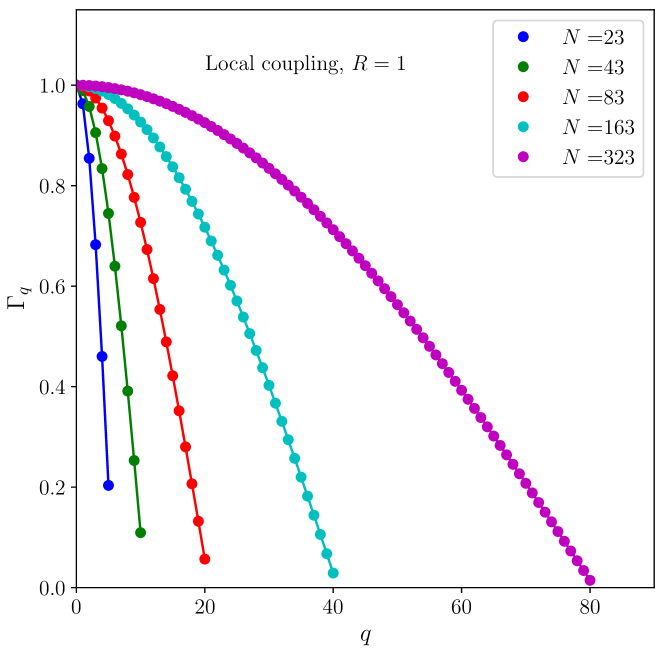
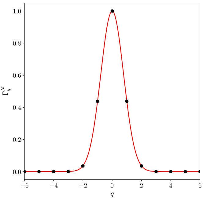
Figure 1: (a) Dependence of $\Gamma_{q}$ with the winding number $q$, for different network sizes. By comparing this plot with that in Fig.3 (inset) of Ref. Delabays2017 , one can notice that $\Gamma_{q}$ behaves as the linear size of the basin of attraction of the $q$ states. (b) Plot of $\Gamma_{q}^{N}$, for $N=60$ and $R=2$ (black circles), and the fitted Gaussian curve (red line).

Then we define $\Gamma_{q}$, the equilibrium stability measure, as the sum of the eigenvalues of a $q$-twisted state, normalized by the most negative $\hat{\gamma}_{q}$ which in this case is $\hat{\gamma}_{0}$:

$$\Gamma_{q}\equiv\frac{\hat{\gamma}_{q}}{\hat{\gamma}_{0}}\,.$$ (5)

We present in Fig. 1(a) the plot of $\Gamma_{q}$ with respect to $q$ for different network sizes with local coupling ($R=1$). (hyperbolic) stable states, i.e. those with $\gamma_{\ell}<0,\forall\,\ell$, were taken into account. It is remarkable the similarity between the plot of $\Gamma_{q}$ and the plot of $\alpha_{\tau}(q)$, the typical linear size of the basin of attraction presented in Fig. 3 (inset) of Ref. Delabays2017 . Therefore, if $\Gamma_{q}$ has a behavior similar to the linear size of a basin of attraction, it is reasonable to expect that for a network with $N$ oscillators the volume of the basin of attraction of a given $q$-state will behave as $\sim\Gamma_{q}^{N}$. In Fig. 1(b) we plot $\Gamma_{q}^{N}$, for $N=60$ and $R=2$; that can be well approximated by a Gaussian curve. To establish this result, in the next subsection we show explicitly for low values of $R/N$ that $\Gamma_{q}^{N}$ can be approximated by a Gaussian function with respect to the winding number $q$, .

The Gaussian distribution of the basins of attraction

Our goal here is to derive an explicit expression for the standard deviation $\sigma$ in terms of the number of nodes $N$ and the connection $R$ of the network. Considering $G=1/N$, Eq. (3) returns

$$\gamma_{\ell}(q)=-4\,\sum_{k=1}^{R}\,\frac{1}{N}\,\cos(k\,q\,\delta)\,\sin^{2}(k\,\ell\,\delta/2)\,,$$ (6)

where $\ell=1,2,\dots,N-1$ and $\delta=2\pi/N$.

By using trigonometric identities, Eq. (6) can be rewritten as

$$\gamma_{\ell}(q)= -\frac{1}{N}\,\sum_{k=1}^{R}\,\{2\cos(k\,q\,\delta)\,-\cos(k\,\delta\,(q+\ell))$$

$$-\cos(k\,\delta\,(q-\ell))\}\,,$$ (7)

and on performing the summations one obtains

$$\gamma_{\ell}(q)= -\frac{1}{N}\,\left\{\frac{\sin\left(M\,q\,\pi/N\right)}{\sin\left(q\,\pi/N\right)}-\frac{1}{2}\left[\frac{\sin\left(M\,(q+\ell)\,\pi/N\right)}{\sin\left((q+\ell)\,\pi/N\right)}\right.\right.$$

$$\left.\left.+\frac{\sin\left(M\,(q-\ell)\,\pi/N\right)}{\sin\left((q-\ell)\,\pi/N\right)}\right]\right\}\,,$$ (8)

where $M\equiv 2R+1$.

Now let us evaluate $\hat{\gamma}_{q}=\sum_{\ell}\gamma_{\ell}(q)$. The summation of the first term in the RHS of Eq. (8) is trivial, but for the second and the third terms, the sums are approximated by integrals since we are regarding $N\gg R,\,q$ :

$$B_{\pm}= \sum_{\ell=1}^{N-1}\,\frac{1}{N}\,\frac{\sin\left(M\,(q\pm\ell)\,\pi/N\right)}{\sin\left((q\pm\ell)\,\pi/N\right)}$$

$$\approx \int_{0}^{1-\varepsilon}\frac{\sin\left(M\,(y\pm x)\,\pi\right)}{\sin\left((y\pm x)\,\pi\right)}dx\,,$$ (9)

where $\varepsilon=1/N$, $x=\ell/N$, $y=q/N$ and $M=2R+1$. Then one arrives at

$$\hat{\gamma}_{q}=1-\frac{\sin\left(M\,y\,\pi\right)}{\sin\left(y\,\pi\right)}+\mathcal{O}(\varepsilon^{2})\,.$$ (10)

In turn, the normalized sum of eigenvalues $\Gamma_{q}$, can be expanded around $y\sim 0$

$$\Gamma_{q} = 1-\frac{\pi^{2}}{3}(2R+1)(R+1)\,y^{2}+\dots\,$$ (11)

$$\approx 1-\beta\frac{q^{2}}{N}\,,$$

where

$$\beta=\frac{\pi^{2}}{3}\frac{(2R+1)(R+1)}{N}\,.$$ (12)

For $N\gg R,q$, the quantity $\Gamma_{q}^{N}$ can be approximated by a Gaussian function

$$\Gamma_{q}^{N}\approx\left(1-\beta\frac{q^{2}}{N}\right)^{N}\approx e^{\displaystyle-\beta q^{2}}\,,$$ (13)

with standard deviation equal to $1/{\sqrt{2\beta}}$. As a result, the standard deviation can be written as

$$\sigma_{T}=\sqrt{N}\,\mathcal{F}(R),\quad\mathcal{F}(R)=\left[\frac{3}{2\pi^{2}(2R+1)(R+1)}\right]^{1/2}.$$ (14)

II Comparison with available numerical data

To compare this result [Eq. (14)] with the one known from the literature Wiley2006 , we restrict ourselves to small values of $R$ and obtain the following expansion for $\sigma_{T}$

$$\sigma_{T} \approx \frac{4\sqrt{3}}{1369\pi}\left(125\frac{1}{\sqrt{R}}-26\right)\sqrt{N}$$ (15)

$$\approx 0.2014\sqrt{\frac{N}{R}}-0.04188\sqrt{N}\,,$$

which has approximately the same scaling law ($\sigma\sim 0.2\sqrt{N/R}$) of the volume of the basin of attraction obtained through numerical experiments. It is important to remark that those experiments were carried out with datasets from different network sizes. But, as we can see, the second term of Eq.(15) is almost negligible and does not differ much for small values of $N$. Therefore, $\sigma$ can be interpreted as linearly dependent on $\sqrt{N/R}$ as argued in Wiley2006 . Nevertheless, Eq.(15) indicates that actually $\sigma/\sqrt{N}$ increases (almost) linearly with $1/\sqrt{R}$.

In Fig.2 we can observe a qualitative agreement (same scaling $\sigma\sim 0.2\sqrt{N/R}$) between the theoretical standard deviation Eq.(14) and numerical experiments for different network sizes, with $R/N\lesssim 0.1$. Furthermore, a good agreement between theory and experimental data can be obtained by adding a constant $\varepsilon$ ($\approx 0.028$) to $\mathcal{F}(R)$ in Eq.(14), as illustrated by the gray dashed line in Fig.2. Then, based on the eigenvalues of equilibrium states, a good estimate for the standard deviation of the distribution of volumes of basins of attraction can be written as

$$\frac{\sigma}{\sqrt{N}} = \mathcal{F}(R)\,+\,\varepsilon$$ (16)

$$= \left[\frac{3}{2\pi^{2}(2R+1)(R+1)}\right]^{1/2}\,+\,\varepsilon\,.$$

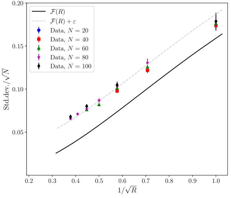
Figure 2: Standard deviation of the distribution of volumes of basins of attraction, divided by $\sqrt{N}$. The blue, red, green, magenta and black marks refer, respectively, to numerical experiments performed in networks with $N=20,40,60,80,$ and 100 with $R/N\lesssim 0.1$. The solid black line is the theoretical result given by Eq. (14). Gray dashed line: a good agreement between our results and experimental data could be obtained by adding a constant $\varepsilon\approx 0.028$ to $\mathcal{F}(R)$.

III Final Remarks

Based on recent mathematical results that establish relationships between global and local properties of nonlinear flows on compact manifolds DangRiviere2019 ; mauroy2016 and also on the observation that the size of the basin of attraction of a $q$–twisted state is correlated with its eigenvalues Ochab2010 , we define the stability measure $\Gamma_{q}$ as proportional to the sum of eigenvalues of the $q$ states and observe that $\Gamma_{q}$ (our Fig. 1(a)) behaves similarly to the linear basin size $\alpha_{\tau}(q)$ (see inset of Fig. 3 in Ref. Delabays2017 ). Then for small $q,R\ll N$, we found an analytic expression for $\Gamma_{q}^{N}$, a Gaussian distribution for $q$ with standard deviation that scales as $\sim 0.2\sqrt{N/R}$, the same behavior obtained by numerical simulations in Ref. Wiley2006 . In Fig. 2 we showed that a good agreement between our theoretical result and experimental data could be obtained by adding a small constant $\varepsilon$, Eq. (16). This indicates that $\Gamma_{q}^{N}$ (obtained from the equilibria eigenvalues) is successful in capturing how the basin volumes are distributed according to the size $N$ and the topology $R$ of the network.

A priori it is not expected that global dynamical properties can be obtained from local characteristics, such as the Jacobian eigenvalues. But our results indicate that some global properties of the system (1) are somehow reflected/encoded in the (local) eigenvalues of the equilibria and is compatible with results about global dynamics of Morse-Smale gradient systems DangRiviere2019 . On the other hand, we suspect that some facts contribute to $\Gamma_{q}^{N}$ having many characteristics identical to the distribution of basins of attraction of the $q$-twisted states. The phase space of the system (1) is

• a compact manifold: an $N$-torus,

• “smooth” because, as pointed out in Ref. Wiley2006 , the system (1) features gradient dynamics with trajectories flowing monotonically over a potential surface and asymptotically reaching fixed points, both in forward and backward time. No complicated behavior (limit cycles, attracting tori, strange attractors, etc.) occurs.

• most likely the basins are well-defined regions in the phase space, separated by smooth high-dimensional hypersurfaces: segments of codimension-1 stable manifolds of the equilibria that possess just one positive Jacobian eigenvalue. These segments are matched on codimension-2 stable manifolds of the equilibria with two positive eigenvalues, and so on. Moreover, in high-dimensional convex bodies the bulk of the volume lies in the immediate vicinity of the boundaries: for a 40-dimensional sphere with radius $R$ or a cube with the size $2R$ the thin boundary layer $0.9R<|r|<R$ contains over 98% of the volume. Therefore, regions of the phase space adjacent to the basin boundaries are responsible for the dominating part of the basin volume. Such geometry favors the long distance linear behavior. We do not expect these results to replay in systems with complicated basins of attraction delimited by fractal, riddled, or Wada boundaries.

Our approach has revealed that certain global phenomena in networks of phase oscillators can be understood by local studies where the dynamics is strongly dominated by attractive and repulsive interactions between the nodes. In such systems the action of the eigenvalues predicting the dynamics protrudes over large distances from the equilibrium state, whether an attractor, a saddle or a repeller, as shown in Mihara2019 . Therefore, we hope that this study can be extended to other network systems with similar features (high-dimensional, with phase space that is a compact manifold, etc.) mainly for the case of Morse-Smale gradient systems with a finite number of hyperbolic equilibrium states.

References

- (1) A. T. Winfree, “Biological rhythms and the behavior of populations of coupled oscillators,” J. Theor. Biol., vol. 16, p. 15, 1967.
- (2) Y. Kuramoto, “Self-entrainment of a population of coupled non-linear oscillators,” in International symposium on mathematical problems in theoretical physics, pp. 420–422, Springer, 1975.
- (3) Y. Kuramoto, Chemical Oscillations, Waves, and Turbulence. Berlin: Springer-Verlag, 1984.
- (4) B. Ermentrout, “An adaptive model for synchrony in the firefly pteroptyx malaccae,” J. Math. Biol., vol. 29, p. 571, 1991.
- (5) T. M. Antonsen Jr, R. T. Faghih, M. Girvan, E. Ott, and J. Platig, “External periodic driving of large systems of globally coupled phase oscillators,” Chaos, vol. 18, p. 037112, 2008.
- (6) K. P. O’Keeffe, H. Hong, and S. H. Strogatz, “Oscillators that sync and swarm,” Nat. Commun., vol. 8, p. 1504, 2017.
- (7) M. Osaka, “Modified Kuramoto phase model for simulating cardiac pacemaker cell synchronization,” Appl. Math., vol. 8, p. 1227, 2017.
- (8) K. Wiesenfeld, P. Colet, and S. H. Strogatz, “Frequency locking in Josephson arrays: Connection with the Kuramoto model,” Phys. Rev. E, vol. 57, p. 1563, 1998.
- (9) F. Dörfler, M. Chertkov, and F. Bullo, “Synchronization in complex oscillator networks and smart grids,” Proc. Natl. Acad. Sci. U.S.A., vol. 110, p. 2005, 2013.
- (10) S. H. Strogatz, D. M. Abrams, A. McRobie, B. Eckhardt, and E. Ott, “Theoretical mechanics: Crowd synchrony on the millennium bridge,” Nature, vol. 438, p. 43, 2005.
- (11) E. Ott, Chaos in dynamical systems. Cambridge university press, 2002.
- (12) D. A. Wiley, S. H. Strogatz, and M. Girvan, “The size of the sync basin,” Chaos, vol. 16, p. 015103, 2006.
- (13) R. Delabays, M. Tyloo, and P. Jacquod, “The size of the sync basin revisited,” Chaos, vol. 27, p. 103109, 2017.
- (14) J. Ochab and P. F. Góra, “Synchronization of coupled oscillators in a local one-dimensional Kuramoto model,” Acta Phys. Pol. B [Proceedings Supplement 3], vol. 3, p. 453, 2010.
- (15) P. J. Menck, J. Heitzig, N. Marwan, and J. Kurths, “How basin stability complements the linear-stability paradigm,” Nat. Phys., vol. 9, p. 89, 2013.
- (16) M. H. Matheny, J. Emenheiser, W. Fon, and et al, “Exotic states in a simple network of nanoelectromechanical oscillators,” Science, vol. 363, p. eaav7932, 2019.
- (17) A. Mihara and R. O. Medrano-T, “Stability in the Kuramoto–Sakaguchi model for finite networks of identical oscillators,” Nonlinear Dyn., vol. 98, pp. 539–550, 2019.
- (18) T. Girnyk, M. Hasler, and Y. Maistrenko, “Multistability of twisted states in non-locally coupled kuramoto-type models,” Chaos: An Interdisciplinary Journal of Nonlinear Science, vol. 22, p. 013114, 03 2012.
- (19) A. Mauroy, I. Mezić and Y. Susuki, The Koopman Operator in Systems and Control, Lect. Notes Control and Information Sciences, vol. 484, Springer, 2020. https://doi.org/10.1007/978-3-030-35713-9.
- (20) N.V. Dang and G. Rivière, Spectral analysis of Morse-Smale gradient flows, Ann. Scient. Éc. Norm. Sup. vol. 52, p. 1403, 2019. http://doi.org/10.24033/asens.2412.
- (21) A. Mauroy and I. Mezić, Global Stability Analysis Using the Eigenfunctions of the Koopman Operator, IEEE Transactions on Automatic Control, vol. 61, p. 3356-3369, 2016. https://doi.org/10.1109/TAC.2016.2518918.
- (22) Y. Takahashi, Entropy Functional (free energy) for Dynamical Systems and their Random Perturbations, North-Holland Mathematical Library, vol. 32, p. 437-467, Elsevier, 1984. https://doi.org/10.1016/S0924-6509(08)70404-5.