Wasserstein Generative Learning of
Conditional Distribution

Abstract

Conditional distribution is a fundamental quantity for describing the relationship between a response and a predictor. We propose a Wasserstein generative approach to learning a conditional distribution. The proposed approach uses a conditional generator to transform a known distribution to the target conditional distribution. The conditional generator is estimated by matching a joint distribution involving the conditional generator and the target joint distribution, using the Wasserstein distance as the discrepancy measure for these joint distributions. We establish non-asymptotic error bound of the conditional sampling distribution generated by the proposed method and show that it is able to mitigate the curse of dimensionality, assuming that the data distribution is supported on a lower-dimensional set. We conduct numerical experiments to validate proposed method and illustrate its applications to conditional sample generation, nonparametric conditional density estimation, prediction uncertainty quantification, bivariate response data, image reconstruction and image generation. image generation and reconstruction.

Keywords: Conditional distribution; Generative learning; Neural Networks; Non-asymptotic error bounds; Nonparametric estimation.

1 Introduction

Conditional distribution is a fundamental quantity for measuring how a response variable $Y$ depends on a predictor $X$. Unlike regression methods that only model certain aspects of the relationship between $Y$ and $X$, such as the conditional mean, conditional distribution provides a complete description of the relationship. In this paper, we propose a nonparametric generative approach to learning a conditional distribution. This approach uses a function, which we shall refer to as a conditional generator, that transforms a known reference distribution to the target conditional distribution. The conditional generator is estimated by matching the joint distribution involving the conditional generator and the predictor and the joint distribution of the response and the predictor. We use the Wasserstein distance as the discrepancy measure for matching these joint distributions.

There is a vast literature on nonparametric conditional density estimation. Many existing methods use smoothing techniques, including kernel smoothing and local polynomials (Rosenblatt,, 1969; Scott,, 1992; Fan et al.,, 1996; Hyndman et al.,, 1996; Hall and Yao,, 2005; Bott and Kohler,, 2017). Basis expansion methods have also been developed for nonparametric conditional density estimation (Izbicki and Lee,, 2016; Izbicki et al.,, 2017). A common feature of these methods is that they seek to estimate the functional form of the conditional density. However, these existing conditional density estimation methods do not work well with high-dimensional complex data. In addition, most existing methods only consider the case when the response $Y$ is a scalar and is not applicable to the settings when $Y$ is a high-dimensional response vector.

The proposed approach is inspired by the generative adversarial networks (GAN) (Goodfellow et al.,, 2014) and Wasserstein GAN (WGAN) (Arjovsky et al.,, 2017). These methods were developed to learn high-dimensional (unconditional) distributions nonparametrically. Instead of estimating the functional forms of density functions, GAN and WGAN start from a known reference distribution and use a function that pushes the reference distribution to the data distribution. In practice, this function, often referred to as a generator, is usually parameterized using deep neural networks. In GAN and WGAN, it is only necessary to estimate a single generator function for sampling from a (unconditional) distribution. However, to sample from a conditional distribution, the generator function necessarily depends on the given value of $X$ to be conditioned on. Since it is difficult to estimate a collection of generator functions for all the possible values of $X$, an effective approach is to formulate the generator function as a map from the product space of the spaces of the reference distribution and $X$ to the space of $Y$. The existence of such a map is guaranteed by the noise-outsourcing lemma in probability theory (Kallenberg,, 2002).

Several authors have generalized GANs to the setting of learning a conditional distribution. Mirza and Osindero, (2014) proposed conditional generative adversarial networks (cGAN). Similar to GANs, it solves a two-player minimax game using an objective function with the same form as that of the original GAN (Goodfellow et al.,, 2014). Kovachki et al., (2021) proposed a conditional sampling approach with monotone GANs. A limitation of this approach is that it requires the dimension of the reference distribution to be the same as the dimension of $Y$. In the high-dimensional settings, this does not allow the exploration of a possible low-dimensional latent structure in the data. Zhou et al., (2021) proposed a generative approach to conditional sampling based on the noise-outsourcing lemma and distribution matching. The Kullback-Liebler divergence is used for matching the generator distribution and the data distribution. They established consistency of the conditional sampler with respect to the total variation distance, with the help of Pinsker’s inequality that bounds the total variation distance via the Kullback-Liebler divergence (Tsybakov,, 2008). However, it is difficult to establish the convergence rate of the conditional sampling distribution with the Kullback-Liebler divergence.

Although the Kullback-Liebler divergence is an attractive discrepancy measure for distributions, it has some drawbacks in the present setting (Arjovsky et al.,, 2017). First, the Kullback-Liebler divergence is a strong divergence measure, for example, it is stronger than the Jensen-Shannon divergence and the total variation distance. Weak convergence of distributions does not imply their convergence in Kullback-Liebler divergence. Second, in high-dimensional problems, we are often interested in learning distributions with a low-dimensional latent structure, whose density functions may not exist. In this case, it is not sensible to use the Kullback-Liebler divergence. In contrast, the Wasserstein distance metricizes the space of probability distributions under mild conditions. This enables us to obtain the non-asymptotic error bounds of the proposed method and its convergence rate, see Theorems 3.1 and 3.2 in Section 3.1. Since the computation of the proposed method does not involve density functions, we can use it to learn distributions without a density function, such as distributions supported on a set with a lower intrinsic dimension than the ambient dimension. We show that the proposed method has an improved convergence rate under a low-dimensional support assumption and can mitigate the curse of dimensionality, see Theorem 3.4 in Section 3.2.

The proposed method for learning a conditional distribution has several appealing properties compared with the standard conditional density estimation methods. First, the proposed method can use a reference distribution with a lower dimension than that of the target distribution, therefore, it can learn conditional distributions with a lower-dimensional latent structure by using a low-dimensional reference distribution. Second, there is no restriction on the dimensionality of the response variable, while the standard methods typically only consider the case of a scalar response variable. Third, the proposed method allows continuous, discrete and mixed types of predictors and responses, while the smoothing and basis expansion methods only deal with continuous-type variables. Finally, since the computation of Wasserstein distance does not involve density functions, it can be used as a loss function for learning distributions without a density function, such as distributions supported on a set with a lower intrinsic dimension than the ambient dimension. Also, by using the Wassertein distance, we are able to establish the non-asymptotic error bound of the generated sampling distribution. To the best of our knowledge, this is the first error bound result in the context of conditional generative learning.

The remainder of this paper is organized as follows. In Section 2 we present the proposed method. In Section 3 we establish the non-asymptotic error bounds for the generated sampling distribution by the proposed method. in terms of the Dudley metric. We also show that the proposed method is able to mitigate the curse of dimensionality under the assumption that the joint distribution of $(X,Y)$ is supported on a set with a low Minkowski dimension. In Section 4 we desribe the implementation of the proposed method. In Section 5 we conduct numerical experiments to validate the proposed method and illustrate its applications in conditional sample generation, nonparametric conditional density estimation, visualization of multivariate data, image generation and image reconstruction. Concluding remarks are given in Section 6. Additional numerical experiment results and the technical details are given in the appendices.

2 Method

We first describe an approach to representing a conditional distribution via a conditional generator function based on the noise-outsoucing lemma. We then describe the proposed method based on matching distributions using Wasserstein metric.

2.1 Conditional sampling based on noise outsourcing

Consider a pair of random vectors $(X,Y)\in\mathcal{X}\times\mathcal{Y}$, where $\mathcal{X}\subseteq\mathbb{R}^{d}$ and $\mathcal{Y}\subseteq\mathbb{R}^{q}.$ Suppose $(X,Y)\sim P_{X,Y}$ with marginal distributions $X\sim P_{X}$ and $Y\sim P_{Y}$. Denote the conditional distribution of $Y$ given $X$ by $P_{Y\mid X}$. For a given value $x$ of $X$, we also write the conditional distribution as $P_{Y\mid X=x}$. For regression problems, $\mathcal{Y}\subseteq\mathbb{R}^{q}$ with $q\geq 1$; for classification problems, $\mathcal{Y}$ is a set of finitely many labels. We assume $\mathcal{X}\subseteq\mathbb{R}^{d}$ with $d\geq 1$. The random vectors $X$ and $Y$ can contain both continuous and categorical components. Let $\eta\in\mathbb{R}^{m}$ be a random vector independent of $(X,Y)$ with a known distribution $P_{\eta}$ that is easy to sample from, such as a normal distribution.

We are interested in finding a function $G:\mathbb{R}^{m}\times\mathcal{X}\mapsto\mathcal{Y}$ such that the conditional distribution of $G(\eta,X)$ given $X=x$ equals the conditional distribution of $Y$ given $X=x$. Since $\eta$ is independent of $X$, this is equivalent to finding a $G$ such that

$$G(\eta,x)\sim P_{Y\mid X=x},\ x\in\mathcal{X}.$$ (2.1)

Therefore, to sample from the conditional distribution $P_{Y\mid X=x}$, we can first sample an $\eta\sim P_{\eta}$ and calculate $G(\eta,x)$, then the resulting $G(\eta,x)$ is a sample from $P_{Y\mid X=x}.$ Because of this property, we shall refer to $G$ as a conditional generator. This approach has also been used in Zhou et al., (2021). The existence of such a $G$ is guaranteed by the noise-outsourcing lemma (Theorem 5.10 in Kallenberg, (2002)). For ease of reference, we state it here with a slight modification.

Lemma 2.1.

(Noise-outsourcing lemma). Suppose $\mathcal{Y}$ is a standard Borel space. Then there exist a random vector $\eta\sim N(\mathbf{0},\mathbf{I}_{m})$ for a given $m\geq 1$ and a Borel-measurable function $G:\mathbb{R}^{m}\times\mathcal{X}\to\mathcal{Y}$ such that $\eta$ is independent of $X$ and

$$(X,Y)=(X,G(\eta,X))\ \text{almost surely.}$$ (2.2)

In Lemma 2.1, the noise distribution $P_{\eta}$ is taken to be $N(\mathbf{0},\mathbf{I}_{m})$ with $m\geq 1$, since it is convenient to generate random numbers from a standard normal distribution. It is a simple consequence of the original noise-outsourcing lemma which uses the uniform distribution on $[0,1]$ for the noise distribution. The dimension $m$ of the noise vector does not need to be the same as $q$, the dimension of $Y.$

Because $\eta$ and $X$ are independent, a $G$ satisfies (2.1) if and only if it also satisfies (2.2). Therefore, to construct the conditional generator, we can find a $G$ such that the joint distribution of $(X,G(\eta,X))$ matches the joint distribution of $(X,Y)$. This is the basis of the proposed generative approach described below.

2.2 Wasserstein generative conditional sampler

Let $\Omega$ be a subset of $\mathbb{R}^{k},k\geq 1,$ on which the measures we consider are defined. Let $\mathcal{B}_{1}(\Omega)$ be the set of Borel probability measures on $\Omega$ with finite first moment, that is, the set of probability measures $\mu$ on $\mathbb{R}^{k}$ such that $\int_{\Omega}\|x\|_{1}d\mu(x)<\infty$, where $\|\cdot\|_{1}$ denotes the 1-norm in $\mathbb{R}^{k}$. The $1$-Wasserstein metric is defined as

$$W_{1}(\mu,\nu)=\inf_{\gamma\in\Gamma(\mu,\nu)}\int\|u-v\|_{1}d\gamma(u,v),\ \mu,\nu\in\mathcal{B}_{1}(\Omega),$$ (2.3)

where $\Gamma(\mu,\nu)$ is the set of joint probability distributions with marginals $\mu$ and $\nu.$ The $1$-Wasserstein metric is also known as the earth mover distance. A computationally more convenient form of the 1-Wasserstein metric is the Monge-Rubinstein dual (Villani,, 2008),

$$W_{1}(\mu,\nu)=\sup_{f\in\mathcal{F}^{1}_{\text{Lip}}}\left\{\mathbb{E}_{U\sim\mu}f(U)-\mathbb{E}_{V\sim\nu}f(V)\right\}.$$ (2.4)

where $\mathcal{F}^{1}_{\text{Lip}}$ is the $1$-Lipschitz class,

$$\mathcal{F}^{1}_{\text{Lip}}=\{f:\mathbb{R}^{k}\to\mathbb{R},|f(u)-f(v)|\leq\|u-v\|_{2},\ u,v\in\Omega\}.$$ (2.5)

When only random samples from $\mu$ and $\nu$ are available in practice, it is easy to obtain the empirical version of (2.4).

We apply the $1$-Wasserstein metric (2.4) to the present conditional generative learning problem, that is, we seek a conditional generator function $G:\mathbb{R}^{m}\times\mathcal{X}\to\mathbb{R}^{q}$ satisfying (2.1). The basic idea is to formulate this problem as a minimisation problem based on the $1$-Wasserstein metric. By Lemma 2.1, we can find a conditional generator $G$ by matching the joint distributions $P_{X,G(\eta,X)}$ and $P_{X,Y}.$ By (2.4), the 1-Wasserstein distance between $P_{X,G(\eta,X)}$ and $P_{X,Y}$ is

$$W_{1}(P_{X,G(\eta,X)},P_{X,Y})=\sup_{D\in\mathcal{F}^{1}_{\text{Lip}}}\left\{\mathbb{E}_{(X,\eta)\sim P_{X}P_{\eta}}D(X,G(\eta,X))-\mathbb{E}_{(X,Y)\sim P_{X,Y}}D(X,Y)\right\}.$$

We have $W_{1}(P_{X,G(\eta,X)},P_{X,Y})\geq 0$ for every measurable $G$ and $W_{1}(P_{X,G(\eta,X)},P_{X,Y})=0$ if and only if $P_{X,G(\eta,X)}=P_{X,Y}.$ Therefore, a sufficient and necessary condition for

$$G^{*}\in\operatorname*{argmin}_{G\in\mathcal{G}}W_{1}(P_{X,G(\eta,X)},P_{X,Y}),$$

is $P_{X,G^{*}(\eta,X)}=P_{X,Y}$, which implies $G^{*}(\eta,x)\sim P_{Y\mid X=x},x\in\mathcal{X}.$ It follows that the problem of finding the conditional generator can be formulated as the minimax problem:

$$\operatorname*{argmin}_{G\in\mathcal{G}}\operatorname*{argmax}_{D\in\mathcal{F}^{1}_{\text{Lip}}}\mathcal{L}(G,D),$$

where

$$\mathcal{L}(G,D)=\mathbb{E}D(X,G(\eta,X))-\mathbb{E}D(X,Y).$$ (2.6)

Let $\{(X_{i},Y_{i}),i=1,\ldots,n\}$ be a random sample from $P_{X,Y}$ and let $\{\eta_{i},i=1,\ldots,n\}$ be independently generated from $P_{\eta}$. The empirical version of $\mathcal{L}(G,D)$ based on $(X_{i},Y_{i},\eta_{i}),i=1,\ldots,n,$ is

$$\mathcal{L}_{n}(G,D)= \frac{1}{n}\sum_{i=1}^{n}D(X_{i},G(\eta_{i},X_{i}))-\frac{1}{n}\sum_{i=1}^{n}D(X_{i},Y_{i}).$$ (2.7)

We use a feedforward neural network $G_{{\bm{\theta}}}$ with parameter ${\bm{\theta}}$ for estimating the conditional generator G and a second network $D_{{\bm{\phi}}}$ with parameter ${\bm{\phi}}$ for estimating the discriminator $D$. We refer to Goodfellow et al., (2016) for a detailed description of neural network functions. We estimate ${\bm{\theta}}$ and ${\bm{\phi}}$ by solving the minimax problem:

$$(\hat{{\bm{\theta}}},\hat{{\bm{\phi}}})=\operatorname*{argmin}_{{\bm{\theta}}}\operatorname*{argmax}_{{\bm{\phi}}}\mathcal{L}_{n}(G_{{\bm{\theta}}},D_{{\bm{\phi}}}).$$ (2.8)

The estimated conditional generator is $\hat{G}=G_{\hat{{\bm{\theta}}}}$ and the estimated discriminator is $\hat{D}=D_{\hat{{\bm{\phi}}}}$.

We show below that for $\eta\sim P_{\eta}$, $\hat{G}(\eta,x)$ converges in distribution to the conditional distribution $P_{Y\mid X=x},x\in\mathcal{X}$. Therefore, we can use $\hat{G}$ to learn this conditional distribution. Specifically, for an integer $J>1$, we generate a random sample $\{\eta_{j},j=1,\ldots,\eta_{J}\}$ from the reference distribution $P_{\eta}$ and calculate $\{\hat{G}(\eta_{j},x),j=1,\ldots,J\}$, which are approximately distributed as $P_{Y\mid X=x}.$ Since generating random samples from $P_{\eta}$ and calculating $\hat{G}(\eta_{j},x)$ are inexpensive, the computational cost is low once $\hat{G}$ is obtained. For $Y\in\mathbb{R}$, this immediately leads to the estimated conditional quantiles of $P_{Y\mid X=x}.$ Moreover, for any function $g:\mathcal{Y}\to\mathbb{R}^{k}$, by the noise outsourcing lemma, we have $\mathbb{E}(g(Y)\mid X=x)=\mathbb{E}g(G(\eta,x)).$ We can estimate this conditional expectation by $n^{-1}\sum_{j=1}^{J}g(\hat{G}(\eta_{j};x)).$ In particular, the conditional mean and conditional variance of $P_{Y\mid X=x}$ can be estimated in a straightforward way. In Section 5 below, we illustrate this approach with a range of examples.

3 Non-asymptotic error analysis

We establish the non-asymptotic error bound for the proposed method in terms of the integral probability metric (Müller,, 1997)

$$d_{\mathcal{F}^{1}_{B}}(P_{XG},P_{X,Y})=\sup_{f\in\mathcal{F}^{1}_{B}}\{\mathbb{E}_{(X,\eta)\sim P_{X}P_{\eta}}f(X,G(\eta,X))-\mathbb{E}_{(X,Y)\sim P_{X,Y}}f(X,Y)\},$$

where $\mathcal{F}^{1}_{B}$ is the uniformly bounded 1-Lipschitz function class,

$$\mathcal{F}^{1}_{B}=\{f:\mathbb{R}^{d+q}\mapsto\mathbb{R},|f(z_{1})-f(z_{2})|\leq\|z_{1}-z_{2}\|,z_{1},z_{2}\in\mathbb{R}^{d+q}\ \text{ and }\|f\|_{\infty}\leq B\}$$

for some constant $0<B<\infty$. The metric $d_{\mathcal{F}_{B}^{1}}$ is also known as the bounded Lipschitz metric ($d_{\text{BL}}$) which metricizes the weak topology on the space of probability distributions. If $P_{X,Y}$ has a bounded support, then $d_{\text{BL}}$ is essentially the same as the 1-Wasserstein distance.

Let $Z=(X,Y)\sim P_{X,Y}$. We make the following assumptions.

Assumption 1.

For some $\delta>0$, $Z$ satisfies the first moment tail condition

$$\mathbb{E}\|Z\|\mathbbm{1}_{\{\|Z\|>\log t\}}=O(t^{-{(\log t)^{\delta}}/{(d+q)}}),\ \text{ for any }t\geq 1.$$

Assumption 2.

The noise distribution $P_{\eta}$ is absolutely continuous with respect to the Lebesgue measure.

These are two mild assumptions. Assumption 1 is a technical condition for dealing with the case when the support of $P_{X,Y}$ is an unbounded subset of $\mathbb{R}^{d+q}.$ It can be shown that Assumption 1 is equivalent to $P(\|Z\|>t)=O(1)({1}/{t})\exp({-t^{1+\delta}/(d+q)}).$ When $P_{X,Y}$ has a bounded support, Assumption 1 is automatically satisfied. Moreover, this assumption is satisfied if $P_{X,Y}$ is subgaussian. Assumption 2 is satisfied by commonly used reference distributions such as the normal distribution.

For the generator network $G_{{\bm{\theta}}}$, we require that

$$\|G_{{\bm{\theta}}}\|_{\infty}\leq\log n.$$ (3.1)

This requirement is satisfied by adding an additional clipping layer $\ell$ after the original output layer of the network,

$$\ell(a)=a\wedge c_{n}\vee(-c_{n})=\sigma(a+c_{n})-\sigma(a-c_{n})-c_{n},$$

where $c_{n}=\log n.$ We truncate the value of $\|G_{\theta}\|$ to an increasing cube $[-\log n,\log n]^{q}$ so that the support of the evaluation function to $[-\log n,\log n]^{d+q}.$ This restricts the evaluation function class to a $2\log n$ domain.

3.1 Non-asymptotic error bound

Let $(L_{1},W_{1})$ be the depth and width of the feedforward ReLU discriminator network $D_{{\bm{\phi}}}$ and let $(L_{2}.W_{2})$ be the depth and width of the feedforward ReLU generator network $G_{{\bm{\theta}}}$. Denote the joint distribution of $(X,\hat{G}(\eta,X))$ by $P_{X,\hat{G}}$.

Theorem 3.1.

Let $(L_{1},W_{1})$ of $D_{{\bm{\phi}}}$ and $(L_{2},W_{2})$ of $G_{{\bm{\theta}}}$ be specified such that $W_{1}L_{1}=\left\lceil\sqrt{n}\right\rceil$ and $W_{2}^{2}L_{2}=cqn$ for some constants $12\leq c\leq 384$. Then, under Assumptions 1 and 2, we have

$$\mathbb{E}_{\hat{G}}d_{\mathcal{F}_{B}^{1}}(P_{X,\hat{G}},P_{X,Y})\leq C(d+q)^{{1}/{2}}n^{-{1}/{(d+q)}}\log n,$$

where $C$ is a constant independent of $(n,d,q)$. Here $\mathbb{E}_{\hat{G}}$ represents the expectation with respect to the randomness in $\hat{G}.$

When $P_{X,Y}$ has a bounded support, we can drop the logarithm factor in the error bound.

Theorem 3.2.

Suppose that $P_{X,Y}$ is supported on $[-M,M]^{d+q}$ for $\infty>M>0$. Let $(L_{1},W_{1})$ of $D_{{\bm{\phi}}}$ and $(L_{2},W_{2})$ of $G_{{\bm{\theta}}}$ be specified such that $W_{1}L_{1}=\left\lceil\sqrt{n}\right\rceil$ and $W_{2}^{2}L_{2}=cqn$ for some constants $12\leq c\leq 384$. Let the output of $G_{\theta}$ be on $[-M,M]^{q}$. Then, under Assumption 2, we have

$$\mathbb{E}_{\hat{G}}d_{\mathcal{F}_{B}^{1}}(P_{X,\hat{G}},P_{X,Y})\leq C({d+q})^{{1}/{2}}n^{-{1}/{(d+q)}},$$

where $C$ is a constant independent of $(n,d,q)$.

The error bound for the conditional distribution follows as a corollary.

Corollary 3.3.

Under the same assumptions and conditions of Theorem 3.2, we have

$$\mathbb{E}_{\hat{G}}\mathbb{E}_{X}d_{\mathcal{F}_{B}^{1}}(P_{\hat{G}(\eta,X)},P_{Y\mid X})\leq C({d+q})^{{1}/{2}}n^{-{1}/{(d+q)}},$$

where $C$ is a constant independent of $(n,d,q)$.

The proofs of Theorems 3.1 and 3.2 and Corollary 3.3 are given in the supplementary material. Assumption 1 only concerns the first moment tail of the joint distribution of $(X,Y)$. Assumption 2 requires the noise distribution to be absolutely continuous with respect to the Lebesgue measure. These assumptions are easily satisfied in practice. Moreover, we have made clear how the prefactor in the error bound depends on the dimension $d+q$ of $(X,Y)$. This is useful in the high-dimensional settings since how the prefactor depends on the dimension plays an important role in determining the quality of the bound. Here the prefactors in the error bounds depend on the dimensions $d$ and $q$ through $(d+q)^{1/2}$. The convergence rate is $n^{-1/(d+q)}$.

Unfortunately, these results suffer from the curse of dimensionality in the sense that the quality of the error bound deteriorates quickly when $d+q$ becomes large. It is generally not possible to avoid the curse of dimensionality without any conditions on the distribution of $(X,Y)$. Detailed discussions on this problem in the context of nonparametric regression using neural networks can be found in Bauer and Kohler, (2019); Schmidt-Hieber, (2020) and Jiao et al., (2021) and the references therein. In particular, Jiao et al., (2021) also provided an analysis of how the prefactor depends on the dimension of $X$. To mitigate the curse of dimensionality, certain assumptions on the distribution of $(X,Y)$ is needed. We consider one such assumption below.

3.2 Mitigating the curse of dimensionality

If the joint distribution of $(X,Y)$ is supported on a low dimensional set, we can improve the convergence rate substantially. Low dimensional structure of complex data have been frequently observed by researchers in image analysis, computer vision and natural language processing, therefore, it is often a reasonable assumption. We use the Minkowski dimension as a measure of the dimensionality of a set (Bishop and Peres,, 2016).

Let $A$ be a subset of $\mathbb{R}^{d}$. For any $\varepsilon>0$, the covering number $\mathcal{N}(\epsilon,A,\|\cdot\|_{2})$ is the minimum number of balls with radius $\varepsilon$ needed to cover $A$ (Van der Vaart and Wellner,, 1996). The upper and the lower Minkowski dimensions of $A\subseteq\mathbb{R}^{d}$ are defined respectively as

$$\dim^{u}_{M}(A) =\limsup_{\epsilon\to 0}\frac{\log\mathcal{N}(\epsilon,A,\|\cdot\|_{2})}{\log(1/\epsilon)},$$

$$\dim^{l}_{M}(A) =\liminf_{\epsilon\to 0}\frac{\log\mathcal{N}(\epsilon,A,\|\cdot\|_{2})}{\log(1/\epsilon)}.$$

If $\dim^{u}_{M}(A)=\dim^{l}_{M}(A)=\dim_{M}(A)$, then $\dim_{M}(A)$ is called the Minkowski dimension or the metric dimension of $A.$

Minkowski dimension measures how the covering number of the set decays when radius of the covering balls goes to 0. When $A$ is a smooth manifold, its Minkowski dimension equals its own topological dimension characterized by the local homeomorphisms. Minkowski dimension can also be used to measure the dimensionality of highly non-regular set, such as fractals (Falconer,, 2004). Nakada and Imaizumi, (2020) and Jiao et al., (2021) have shown that deep neural networks can adapt to the low dimensional structure of the data and mitigate the curse of dimensionality in nonparametric regression. We show similar results can be obtained for the proposed method if the data distribution is supported on a set with low Minkowski dimension.

Assumption 3.

Suppose $P_{X,Y}$ is supported on a bounded set $A\subseteq[-M,M]^{d+q}$ and $\dim_{M}(A)=d_{A}\leq d+q$.

Theorem 3.4.

Suppose that $P_{X,Y}$ is supported on $[-M,M]^{d+q}$ for $M>0$. Let $(L_{1},W_{1})$ of $D_{{\bm{\phi}}}$ and $(L_{2},W_{2})$ of $G_{{\bm{\theta}}}$ be specified such that $W_{1}L_{1}=\left\lceil\sqrt{n}\right\rceil$ and $W_{2}^{2}L_{2}=cqn$ for some constants $12\leq c\leq 384$. Let the output of $G_{{\bm{\theta}}}$ be on $[-M,M]^{q}$. Let the output of $G_{{\bm{\theta}}}$ be on $[-M,M]^{q}$. Then, under Assumptions 2 and 3, we have

$$\mathbb{E}_{\hat{G}}d_{\mathcal{F}_{B}^{1}}(P_{X,\hat{G}},P_{X,Y})\leq C({d+q})^{{1}/{2}}n^{-{1}/{d_{A}}},$$

where $C$ is a constant independent of $(n,d,q)$.

In comparison with Theorem 3.2, where the rate of convergence depends on $d+q$, the convergence rate in Theorem 3.4 is determined by the Minkowski dimension $d_{A}$. Therefore, the assumption of a low Minkowski dimension on the support of data distribution alleviates the curse of dimensionality. However, unless we have better approximation error bounds for Lipschitz functions defined on low Minkowski dimensional set using neural network functions, the prefactor in Theorem 3.4 is still $(d+q)^{1/2}$, that is, even the convergence rate only depends on the Minkowski dimension $d_{A}$, the prefactor still depends on the ambient dimension $d+q.$

4 Implementation

The estimator $(\hat{\bm{\theta}},\hat{\bm{\phi}})$ of the neural network parameter $({\bm{\theta}},{\bm{\phi}})$ is the solution to the minimax problem

$$(\hat{\bm{\theta}},\hat{\bm{\phi}})=\operatorname*{argmin}_{{\bm{\theta}}}\operatorname*{argmax}_{{\bm{\phi}}}\frac{1}{n}\sum_{i=1}^{n}\{D_{\bm{\phi}}(X_{i},G_{{\bm{\theta}}}(\eta_{i},X_{i}))-D_{\bm{\phi}}(X_{i},Y_{i})\}.$$ (4.1)

We use the gradient penalty algorithm to impose the constraint that the discriminator belongs to the class of 1-Lipschitz functions (Gulrajani et al.,, 2017). The minimax problem (4.1) is solved by updating ${\bm{\theta}}$ and ${\bm{\phi}}$ alternately as follows:

• Fix ${\bm{\theta}}$, update the discriminator by maximizing the empirical objective function

  $$\hat{\bm{\phi}}=\operatorname*{argmax}_{{\bm{\phi}}}\frac{1}{n}\sum_{i=1}^{n}\big{\{}D_{\bm{\phi}}(X_{i},\hat{G}_{\bm{\theta}}(\eta_{i},X_{i}))-D_{\bm{\phi}}(X_{i},Y_{i})-\lambda(\|\nabla_{(x,y)}D_{\bm{\phi}}(X_{i},Y_{i})\|_{2}-1)^{2}\big{\}}$$

  with respect to ${\bm{\phi}}$, where $\nabla_{(x,y)}D_{\bm{\phi}}(X_{i},Y_{i})$ is the gradient of $D_{\bm{\phi}}(x,y)$ with respect to $(x,y)$ evaluated at $(X_{i},Y_{i}).$ The third term on the right side is the gradients penalty for the Lipschitz condition on the discriminator (Gulrajani et al.,, 2017).

• Fix ${\bm{\phi}}$, update the generator by minimizing the empirical objective function

  $$\hat{\bm{\theta}}=\operatorname*{argmin}_{{\bm{\theta}}}\frac{1}{n}\sum_{i=1}^{n}\hat{D}_{\bm{\phi}}(X_{i},G_{\bm{\theta}}(\eta_{i},X_{i}))$$

  with respect to ${\bm{\theta}}$.

We implemented this algorithm in TensorFlow (Abadi et al.,, 2016).

We also implemented the weight clipping method for enforcing the Lipschitz condition on the discriminator (Arjovsky et al.,, 2017). With weight clipping, all weights in the discriminator is truncated to be between $[-c,c],$ where $c>0$ is a small number. We found that the gradient penalty method is more stable and converges faster. So we only report the numerical results based on the gradient penalty method below.

5 Numerical experiments

We carry out numerical experiments to evaluate the finite sample performance of the proposed method described in Section 2 and illustrate its applications using examples in conditional sample generation, nonparametric conditional density estimation, visualization of multivariate data, and image generation and reconstruction. Additional numerical results are provided in the supplementary material. For all the experiments below, the noise random vector $\eta$ is generated from a standard multivariate normal distribution. We implemented the proposed method in TensorFlow (Abadi et al.,, 2016) and used the stochastic gradient descent algorithm Adam (Kingma and Ba,, 2015) in training the neural networks.

5.1 Conditional sample generation: the two-moon dataset

We use the two-moon data example to illustrate the use of the proposed method for generating conditional samples. Let $X\in\{1,2\}$ be the class label and let $Y\in\mathbb{R}^{2}$. The two-moon model is

$$Y=\begin{cases}(\cos(\alpha)+\frac{1}{2}+\epsilon_{1},\sin(\alpha)-\frac{1}{6}+\epsilon_{2}),&\text{if $X=1$,}\\ (\cos(\alpha)-\frac{1}{2}+\epsilon_{3},-\sin(\alpha)+\frac{1}{6}+\epsilon_{4}),&\text{if $X=2$,}\end{cases}$$ (5.1)

where $\alpha\sim\text{Uniform}[0,\pi]$, $\epsilon_{1},\ldots,\epsilon_{4}$ are independent and identically distributed as $N(0,\sigma^{2}).$ We generate three sets of random samples of size $n=5,000$ with $2,500$ for each class and $\sigma=0.1,0.2$ and 0.3 from this model. The generated datasets are shown in the first row of Figure 1.

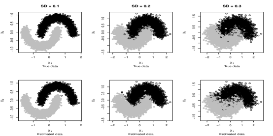
Figure 1: Comparison of simulated data from (5.1) and estimated sample using the proposed method. From the left to the right, each columns corresponds to a different value of the standard deviation in the model with $\sigma=0.1,0.2$ and 0.3, respectively. The first row displays true data and the second row displays the estimated samples.

We use the simulated data to estimate the conditional generator, which is parameterized as a two-layer fully-connected network with 30 and 20 nodes. The discriminator is also a two-layer fully-connected network with 40 and 20 nodes. The noise $\eta\sim N(\mathbf{0},\mathbf{I}_{2}).$ The activation function for the hidden layer of the generator and the discriminator is ReLU. For the output layer of the generator, the activation function is the hyperbolic tangent function. The estimated samples $\{\hat{G}(\eta_{j},x),j=1.\ldots,5,000\}$, $x\in\{1,2\},$ are shown in the second row of Figure 1. It can be seen that the scatter plots of the estimated samples are similar to those of the simulated data. This provides a visual validation of the estimated samples in this toy example.

5.2 Nonparametric conditional density estimation

We consider the problem of estimating conditional mean and conditional standard deviation in nonparametric conditional density models. We also compare the proposed Wasserstein generative conditional sampling method, referred to as WGCS in Table 1, with three existing conditional density estimation methods, including the nearest neighbor kernel conditional density estimator (NNKCDE) (Dalmasso et al.,, 2020), the conditional kernel density estimator (CKDE, implemented in R package np (Hall et al.,, 2004), and a basis expansion method FlexCode (Izbicki et al.,, 2017). We simulated data from the following three models:

• Model 1 (M1). A nonlinear model with an additive error term:

  $$Y=X_{1}^{2}+\exp(X_{2}+X_{3}/3)+\sin(X_{4}+X_{5})+\varepsilon,\ \varepsilon\sim N(0,1).$$

• Model 2 (M2). A model with a multiplicative non-Gassisan error term:

  $$Y=(5+X_{1}^{2}/3+X_{2}^{2}+X_{3}^{2}+X_{4}+X_{5})*\exp(0.5\times\varepsilon),$$

  where $\varepsilon\sim 0.5N(-2,1)+0.5N(2,1).$

• Model 3 (M3). A mixture of two normal distributions:

  $$Y=\mathbb{I}_{\{U\leq{1}/{3}\}}N(-1-X_{1}-0.5X_{2},0.5^{2})+\mathbb{I}_{\{U>{1}/{3}\}}N(1+X_{1}+0.5X_{2},1),$$

  where $U\sim\text{Unif}(0,1)$ and is independent of $X$.

In each model, the covariate vector $X$ is generated from $N(\mathbf{0},\mathbf{I}_{100})$. So the ambient dimension of $X$ is 100, but (M1) and (M2) only depend on the first 5 components of $X$ and (M3) only depends on the first 2 components of $X$. The sample size $n=5,000$.

For the proposed method, the conditional generator $G$ is parameterized using a one-layer neural network in models (M1) and (M2); it is parameterized by a two-layer fully connected neural network in (M3). The discriminator $D$ is parameterized using a two-layer fully connected neural network. The noise vector $\eta\sim N(0,1).$

For the conditional density estimation method NNKCDE, the tuning parameters are chosen using cross-validation. The bandwidth of the conditional kernel density estimator CKDE is determined based on the standard formula $h_{j}=1.06\sigma_{j}n^{-1/(2k+d)},$ where $\sigma_{j}$ is a measure of spread of the $j$th variable, $k$ the order of the kernel, and $d$ the dimension of $X$. The basis expansion based method FlexCode uses Fourier basis. The maximum number of bases is set to 40 and the actual number of bases is selected using cross-validation.

		WGCS	NNKCDE	CKDE	FlexCode
M1	Mean	1.10(0.05)	2.49(0.01)	3.30(0.02)	2.30(0.01)
	SD	0.24(0.04)	0.43(0.01)	0.59(0.01)	1.06(0.08)
M2	Mean	3.71(0.23)	6.09(0.07)	66.76(2.06)	10.20(0.33)
	SD	3.52(0.17)	9.33(0.23)	18.87(0.59)	11.08(0.34)
	Mean	0.32(0.03)	0.11(0.01)	1.55(0.03)	0.12(0.04)
M3	SD	0.10(0.01)	0.36(0.01)	0.51(0.01)	0.33(0.01)

Table 1: Mean squared error (MSE) of the estimated conditional mean, the estimated standard deviation and the corresponding simulation standard errors (in parentheses). The bold numbers indicate the smallest MSEs. NNKCDE: nearest neighbor kernel conditional density estimator; CKDE: conditional kernel density estimator; FlexCode: basis expansion method; WGCS: Wasserstein generative conditional sampler.

We consider the mean squared error (MSE) of the estimated conditional mean $\mathbb{E}(Y|X)$ and the estimated conditional standard deviation $\text{SD}(Y|X)$. We use a test data set $\{x_{1},\dots,x_{K}\}$ of size $K=2,000$ . For the proposed method, we first generate $J=10,000$ samples $\{\eta_{j}:j=1,\ldots,J\}$ from the reference distribution $P_{\eta}$ and calculate conditional samples $\{\hat{G}(\eta_{j},x_{k}),j=1,\dots,J,k=1,\ldots,K\}$ The estimated conditional standard deviation is calculated as the sample standard deviation of the conditional samples. The MSE of the estimated conditional mean is $\text{MSE(mean)}=(1/K)\sum_{k=1}^{K}\{\hat{\mathbb{E}}(Y|X=x_{k})-\mathbb{E}(Y|X=x_{k})\}^{2}.$ For the proposed method, the estimate of the conditional mean is obtained using Monte Carlo. For other methods, the estimate is calculated by numerical integration. Similarly, the MSE of the estimated conditional standard deviation is $\text{MSE(sd)}=(1/K)\sum_{k=1}^{K}\{\hat{\text{SD}}(Y|X=x_{k})-\text{SD}(Y|X=x_{k})\}^{2}.$ The estimated conditional standard deviation of other methods are computed by numerical integration.

We repeat the simulations 10 times. The average MSEs and simulation standard errors are summarized in Table 1. Comparing with CKDE and FlexCode and NNKCED. WGCS has the smallest MSEs for estimating conditional mean and conditional SD in most cases.

5.3 Prediction interval: the wine quality dataset

We use the wine quality dataset (Cortez et al.,, 2009) to illustrate the application of the proposed method to prediction interval construction. This dataset is available at UCI machine learning repository (https://archive.ics.uci.edu/ml/datasets/Wine+Quality). There are eleven physicochemical quantitative variables including fixed acidity, volatile acidity, citric acid, residual sugar, chlorides, free sulfur dioxide, total sulfur dioxide, density, pH, sulphates, alcohol as predictors and a sensory quantitative variable quality that measures wine quality, which is a score between 0 and 10. The goal is to build a prediction model for the wine quality score based on the eleven physicochemical variables. Such a model can be used to help the oenologist wine tasting evaluations and improve wine production. We use the proposed method to learn the conditional distribution of quality given the eleven variables. An advantage of the proposed method over the standard nonparametric regression is that it provides a prediction interval for the quality score, not just a point prediction.

The sample size of this dataset is 4,898. We use 90% of the samples as the training set and 10% as the test set. All variables are centered and standardized first before training the model. In our proposed method, the conditional generator is a two-layer fully-connected feedforward network with 50 and 20 nodes, the discriminator is a two-layer network with 50 and 25 nodes. The ReLU activation function is used in both networks. The noise $\eta\sim N(\mathbf{0},\mathbf{I}_{3}).$

Figure 2: The prediction intervals for the test set. The actual quality scores of 100 randomly selected wine samples in the test set are shown as the solid dots.

To examine the prediction performance of the proposed method, we construct the 90% prediction interval for the wine quality score in the test set. The prediction intervals are shown in Figure 2. The actual quality scores are plotted as solid dots. The actual coverage for all 490 in the test set is 90.80%, close to the nominal level of 90%.

5.4 Bivariate response: California housing data

We use the California housing dataset to demonstrate that the generated conditional samples from the proposed method can be used for visualizing conditional distributions of bivariate response data. This dataset is available at StatLib repository (http://lib.stat.cmu.edu/datasets/). It contains 20,640 observations on housing prices with 9 covariates including median house value, median income, median house age, total rooms, total bedrooms, population, households, latitude, and longitude. Each row of the data matrix represents a neighborhood block in California. We use the logarithmic transformation of the variables except longitude, latitude and median house age. All columns of the data matrix are centered and standardized to have zero mean and unit variance. The generator is a two-layer fully-connected neural network with 60 and 25 nodes and the discriminator is a two-layer network with 65 and 30 nodes. ReLU activation is used for the hidden layers. The random noise vector $\eta\sim N(\mathbf{0},\mathbf{I}_{4})$.

We train the WGCS model with (median income, median house value) $\in\mathbb{R}^{2}$ as the response vector and other variables as the predictors in the model. We use 18,675 observations (about the 90% of the dataset) as training set and the remaining 2,064 (about 10% of the dataset) observations as the test set.

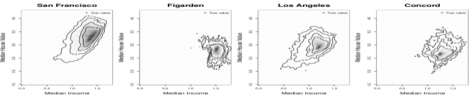
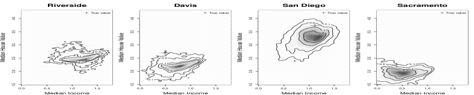
Figure 3: Kernel density estimates of generated conditional samples of median income and median house value (in logarithmic scale) for eight neighborhood blocks in the California Housing dataset. The plus sign “$+$” represents the observed median income and median house values.

Figure 3 shows the contour plot of the conditional distributions of median income and median house value (in logarithmic scale) for 8 single blocks in the test set. The colored density function represents the kernel density estimates based on the samples generated using the proposed method. We see that the blue cross is in the main body of the plot, which shows that the proposed method provides reasonable prediction of the median income and house values. We also see that big cities like San Francisco and Los Angles have higher house values with larger variations, smaller cities such as Davis and Concord tend to have lower house values.

5.5 Image reconstruction: MNIST dataset

We now illustrate the application of the proposed method to high-dimensional data problems and demonstrate that it can easily handle the models when either of both of $X$ and $Y$ are high-dimensional. We use the MNIST handwritten digits dataset (LeCun and Cortes,, 2010), which contains 60,000 images for training and 10,000 images for testing. The images are stored in $28\times 28$ matrices with gray color intensity from 0 to 1. Each image is paired with a label in $\{0,1\dots,9\}$. We use WGCS to perform two tasks: generating images from labels and reconstructing the missing part of an image.

We illustrate using the proposed method for image reconstruction when part of the image is missing with the MNIST dataset. Suppose we only observe ${1}/{4},{1}/{2}$ or ${3}/{4}$ of an image and would like to reconstruct the missing part of the image. For this problem, let $X$ be the observed part of the image and let $Y$ be the missing part of the image. Our goal is to reconstruct $Y$ based on $X$. For discriminator, we use two convolutional networks to process $X$ and $Y$ separately. The filters are then concatenated together and fed into another convolution layer and fully-connected layer before output. For the generator, $X$ is processed by a fully-connected layer followed by 3 deconvolution layers. The random noise vector $\eta\sim N(\mathbf{0},\mathbf{I}_{100}).$

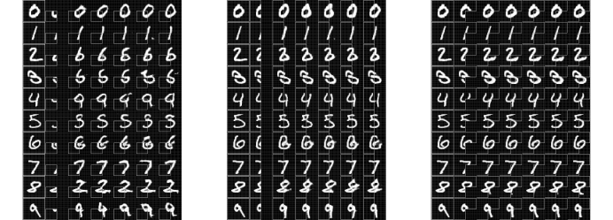
Figure 4: Reconstructed images given partial image in MNIST dataset. The first column in each panel consists of the true images, the other columns give the constructed images. In the left panel, the left lower 1/4 of the image is given; in the middle panel, the left 1/2 of the image is given; in the right panel, 3/4 of the image is given.

In Figure 4, three panels from left to right correspond to the situations when ${1}/{4},{1}/{2}$ or ${3}/{4}$ of an image are given, the problem is to reconstruct the missing part of the image. In each panel, the first column contains the true images in the testing set; the second column shows the observed part of the image; the third to the seventh columns show the reconstructed images. The digits “0”, “1” and “7” are easy to reconstruct, even when only 1/4 of their images are given. For the other digits, if only 1/4 of their images are given, it is difficult to reconstruct them. However, as the given part increases from 1/4 to 1/2 and then 3/4 of the images, the proposed method is able to reconstruct the images correctly, and the reconstructed images become less variable and more similar to the true image. For example, for the digit “2”, if only the left lower 1/4 of the image is given, the reconstructed images tend to be incorrect; the reconstruction is only successful when 3/4 of the image is given.

5.6 Image generation: CelebA dataset

We illustrate the application of the proposed method to the problem of image generation given label information with the CelebFaces Attributes (CelebA) dataset (Liu et al.,, 2015). This dataset contains more then 200K colored celebrity images with 40 attributes annotation. Here we use 10 binary features, including: Gender, Young, Bald, Bangs, Blackhair, Blondhair, Eyeglasses, Mustache, Smiling, WearingNecktie. We take these features as $X$. So $X$ is a vector consisting of 10 binary components. We consider six types of images; the attributes of these six types are shown in Table A.1. We used the aligned and cropped images and further resize them to $96\times 96$ as our training set. We take these colored images as the values of $Y$. Therefore, the dimension of $X$ is 10 and the dimension of $Y$ is $96\times 96\times 3=27,648$.

Attributes	Gender	Young	Blkhair	Bldhair	Glass	Bald	Mus	Smile	Necktie	Bangs
Type 1	F	Y	N	N	N	N	N	Y	N	N
Type 2	F	Y	N	Y	N	N	N	Y	N	N
Type 3	F	Y	Y	N	N	N	N	N	N	N
Type 4	M	Y	N	N	N	N	N	N	N	N
Type 5	M	N	N	N	N	N	N	Y	N	N
Type 6	M	Y	Y	N	N	N	N	Y	N	N

Table 2: Attributes for six types of face images in the CelebA dataset: F$=$Female, M$=$Male; Y$=$ Yes, N$=$ No.

The architecture of the discriminator is specified as follows: the 10 dimensional one-hot vector is first expanded to $96\times 96\times 10$ by replicating each number to a $96\times 96$matrix. Then it is concatenated with image $Y$ on the last axis. Thus the processed data has dimension $96\times 96\times 13$. This processed data is then fed into 5 consecutive convolution layers initialized by truncated normal distribution with $SD=0.01$ with 64,128,256,512,1024 filters respectively. The activation for each convolution layer is a leaky ReLU with $\alpha=0.2$. The strides is 2 and the kernel size is 5. After convolution, it is flattened and connected to a dense layer with one unit as output.

The architecture of the conditional generator is as follows: the noise vector and the feature vector $X$ are concatenated and fed to a dense layer with $3\times 3\times 1024$ units with ReLU activation and then reshaped to $3\times 3\times 1024$. Then it goes through 5 layers of deconvolution initialized by truncated normal distribution with $SD=0.01$ with 512,256,128,64,3 filters respectively. The activation for each intermediate convolution layer is ReLU and hyperbolic tangent function for the last layer. The strides is 2 and kernel size is 5. The optimizer is Adam with $\beta_{1}=0.5$ and learning rate decrease from $0.0001$ to $0.000005$. The noise dimension is 100.

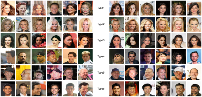
Figure 5: The left panel shows the true images in CelebA dataset. The right panel consists of generated images. Each row corresponds to a specific type of faces.

In Figure 5, the left panel shows real images and the right panel shows generated images. Each row corresponds to a specific type of face. The attributes of the six types of face images are given in Table A.1. We can see that the generated images have similar qualities as the original ones.

6 Discussion

We have proposed a Wasserstein conditional sampler, a generative approach to learning a conditional distribution. We establish the convergence rate of the sampling distribution of the proposed method. We also show that the curse of dimensionality can be mitigated if the data distribution is supported on a lower dimensional set. Our numerical experiments demonstrate that the proposed method performs well in a variety of settings from standard conditional density estimation to more complex image generation and reconstruction problems.

In the future work, it would be interesting to consider incorporating additional information such as sparsity and latent low dimensional structure of data in the proposed method to better deal with the curse of dimensionality in the high-dimensional settings.

Appendices

In the appendices, we include additional numerical results, proofs of the theorems stated in the paper and technical details.

Appendix A Additional numerical results

We carry out numerical experiments to evaluate the finite sample performance of WGCS and illustrate its applications using examples in conditional sample generation, nonparametric conditional density estimation, visualization of multivariate data, and image generation and reconstruction. For all the experiments below, the noise random vector $\eta$ is generated from a standard multivariate normal distribution. The discriminator is updated five times per one update of the generator. We implemented WGCS in TensorFlow (Abadi et al.,, 2016) and used the stochastic gradient descent algorithm Adam (Kingma and Ba,, 2015) in training the neural networks.

A.1 Conditional prediction: the abalone dataset

The abalone dataset is available at UCI machine learning repository (Dua and Graff,, 2017). It contains the number of rings of abalone and other physical measurements. The age of abalone is determined by cutting the shell through the cone, staining it, and counting the number of rings through a microscope, a time-consuming process. Other measurements, which are easier to obtain, are used to predict the number of rings that determines the age. This dataset contains 9 variables. They are sex, length, diameter, height, whole weight, shucked weight, viscera weight, shell weight and rings. Except for the categorical variable sex, all the other variables are continuous. The variable sex codes three groups: female, male and infant, since the gender of an infant abalone is not known. We take rings as the response $Y\in\mathbb{R}$ and the other measurements as the covariate vector $X\in\mathbb{R}^{9}$. The sample size is 4,177. We use 90% of the data for training and 10% of the data as the test set.

The generator is a two-layer fully-connected network with 50 and 20 nodes and the discriminator is also a two-layer network with 50 and 25 nodes, both with ReLU activation function. The noise $\eta\sim N(\mathbf{0},\mathbf{I}_{3}).$

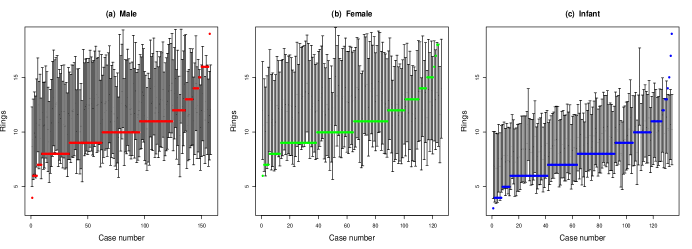
Figure A.1: The prediction intervals for the test set. The 418 abalones in the test set are divided into three groups, (a) male, (b) female, and (c) infant.

To examine the prediction performance of the estimated conditional density, we construct the 90% prediction interval for the number of rings of each abalone in the testing set. The prediction intervals are shown in Figure A.1. The actual number of rings are plotted as a solid dot. The actual coverage for all 418 cases in the testing set is 90.90%, close to the nominal level of 90%. The numbers of rings that are not covered by the prediction intervals are the largest ones in each group. This dataset was also analyzed in Zhou et al., (2021) using a generative method with the Kullback-Liebler divergence measure. The results are similar.

A.2 Image generation: MNIST dataset

We now illustrate the application of WGCS to high-dimensional data problems and demonstrate that it can easily handle the models when either of both of $X$ and $Y$ are high-dimensional. We use the MNIST handwritten digits dataset (LeCun and Cortes,, 2010), which contains 60,000 images for training and 10,000 images for testing. The images are stored in $28\times 28$ matrices with gray color intensity from 0 to 1. Each image is paired with a label in $\{0,1\dots,9\}$. We use WGCS to perform two tasks: generating images from labels and reconstructing the missing part of an image.

We generate images of handwritten digits given the label. In this problem, the predictor $X$ is a categorical variable representing the ten digits: $\{0,1,\dots,9\}$ and the response $Y$ represents $28\times 28$ images. We use one-hot vectors in $\mathbb{R}^{10}$ to represent these ten categories. So the dimension of $X$ is 10 and the dimension of $Y$ is $28\times 28=784.$ The response $Y\in[0,1]^{28\times 28}$ is a matrix representing the intensity values. For the discriminator $D$, we use a convolutional neural network (CNN) with 3 convolution layers with 128, 256, and 256 filters to extract the features of the image and then concatenate with the label information (repeated 10 times to match the dimension of the features). The concatenated information is sent to a fully connected layer and then to the output layer. For the generator $G$, we concatenate the label information with the random noise vector $\eta\sim N(\mathbf{0},\mathbf{I}_{100}).$ Then it is fed to a CNN with 3 deconvolution layers with 256, 128, and 1 filters, respectively.

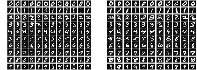
Figure A.2: MNIST dataset: real images (left panel) and generated images given the labels (right panel).

Figure A.2 shows the real images (left panel) and generated images (right panel). We see that the generated images are similar to the real images and it is hard to distinguish the generated ones from the real images. Also, there are some differences in the generated images, reflecting the random variations in the generating process.

A.3 Image generation given labels: CelebA dataset

We illustrate the application of WGCS to the problem of image generation with the CelebFaces Attributes (CelebA) dataset (Liu et al.,, 2015), which is a large-scale dataset containing more then 200K colored celebrity images with 40 attributes annotation. Here we use 10 features including: Gender, Young, Bald, Bangs, Blackhair, Blondhair, Eyeglasses, Mustache, Smiling, WearingNecktie as binary variables. We take these features as $X$. So $X$ is a vector consisting of 10 binary components. We used the aligned and cropped images and further resize them to $96\times 96$ as our training set. We take these colored images as the values of $Y$. Therefore, the dimension of $X$ is 10 and the dimension of $Y$ is $96\times 96\times 3=27,648$.

Attributes	Gender	Young	Blkhair	Bldhair	Glass	Bald	Mus	Smile	Necktie	Bangs
Type 1	F	Y	N	N	N	N	N	Y	N	N
Type 2	F	Y	N	Y	N	N	N	Y	N	N
Type 3	F	Y	Y	N	N	N	N	N	N	N
Type 4	M	Y	N	N	N	N	N	N	N	N
Type 5	M	N	N	N	N	N	N	Y	N	N
Type 6	M	Y	Y	N	N	N	N	Y	N	N

Table A.1: Attributes for six types of face images in the CelebA dataset: F$=$Female, M$=$Male; Y$=$ Yes, N$=$ No.

The architecture of the discriminator is specified as follows: the 10 dimensional one-hot vector is first expanded to $96\times 96\times 10$ by replicating each number to a $96\times 96$matrix. Then it is concatenated with image $Y$ on the last axis. Thus the processed data has dimension $96\times 96\times 13$. This processed data is then fed into 5 consecutive convolution layers initialized by truncated normal distribution with $SD=0.01$ with 64,128,256,512,1024 filters respectively. The activation for each convolution layer is a leaky RELU with $\alpha=0.2$. The strides is 2 and the kernel size is 5. After convolution, it is flattened and connected to a dense layer with one unit as output.

The structure of generator is as follows: the input of $X$ and noise is concatenated and fed to a dense layer with $3\times 3\times 1024$ units with RELU activation and then reshaped to $3\times 3\times 1024$. Then it goes through 5 layers of deconvolution initialized by truncated normal distribution with $SD=0.01$ with 512,256,128,64,3 filters respectively. The activation for each intermediate convolution layer is RELU and hyperbolic tangent function for the last layer. The strides is 2 and kernel size is 5. The optimizer is Adam with $\beta_{1}=0.5$ and learning rate decrease from $0.0001$ to $0.000005$. The noise dimension is 100.

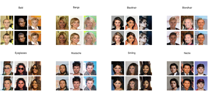
Figure A.3: Comparison of the binary features. All images in this figure are generated images. The first row and second row are generated given the same random noise and attributes except for the one noted above.

In Figure A.3, we present image generation given some specific attributes. All the images in this figure are generated. For each panel, there are three pairs of faces. Each pair is generated with the same $\eta$ except for the feature labeled above so they look exactly the same except for the specified feature. For example, the first panel shows the generate bald or non-bald faces, the first row includes bald faces and the second row includes non-bald faces.

Appendix B A high level description of the error analysis

Below we first present a high level description of the error analysis. For the estimator $\hat{G}$ of the conditional generator as given in (2.8), we are interested in bounding the error $d_{\mathcal{F}^{1}}(P_{X,\hat{G}},P_{X,Y})$. Our basic idea is to decompose this error into terms that are easier to analyze.

Let $\{(X^{\prime}_{i},Y^{\prime}_{i}),i=1,\ldots,n\}$ and $\{\eta^{\prime}_{j},j=1,\ldots,n\}$ be ghost samples that are independent of the original samples. Here we introduce ghost samples as a technical tool for bounding the stochastic error term $\mathcal{E}_{4}$ defined below. The details are given in the proof of Lemma C.7 in the appendix. We consider $(\hat{G},\hat{D})$ based on the empirical version of $\mathcal{L}(G,D)$ that depends on the original samples $(X_{i},Y_{i},\eta_{i})$ given in (2.7) and $(\hat{G}^{\prime},\hat{D}^{\prime})$ based on the loss function of the ghost samples $(X^{\prime}_{i},Y^{\prime}_{i},\eta^{\prime}_{i})$,

$$\mathcal{L}_{n}^{\prime}(G,D)=\frac{1}{n}\sum_{i=1}^{n}D(X^{\prime}_{i},G(\eta^{\prime}_{i},X^{\prime}_{i}))-\frac{1}{n}\sum_{i=1}^{n}D(X^{\prime}_{i},Y^{\prime}_{i}).$$

Recall the error $d_{\mathcal{F}^{1}}(P_{X,\hat{G}},P_{X,Y})$ is defined by

$$d_{\mathcal{F}_{B}^{1}}(P_{X,\hat{G}},P_{X,Y})=\sup_{f\in\mathcal{F}_{B}^{1}}\{\mathbb{E}f(X,\hat{G})-\mathbb{E}f(X,Y)\}.$$

We decompose it as follows:

$$d_{\mathcal{F}_{B}^{1}}(P_{X,\hat{G}},P_{X,Y})\leq\sup_{f\in\mathcal{F}_{B}^{1}}\Big{\{}\mathbb{E}f(X,\hat{G})-\frac{1}{n}\sum_{i=1}^{n}f(X^{\prime}_{i},\hat{G}^{\prime})\Big{\}}$$

$$+\sup_{f\in\mathcal{F}_{B}^{1}}\Big{\{}\frac{1}{n}\sum_{i=1}^{n}f(X^{\prime}_{i},\hat{G}^{\prime})-\frac{1}{n}\sum_{i=1}^{n}f(X^{\prime}_{i},Y^{\prime}_{i})\Big{\}}+\sup_{f\in\mathcal{F}_{B}^{1}}\Big{\{}\frac{1}{n}\sum_{i=1}^{n}f(X^{\prime}_{i},Y^{\prime}_{i})-\mathbb{E}f(X,Y)\Big{\}}$$

$$:=\mathcal{E}_{4}+A+\mathcal{E}3,$$

where $A=\sup_{f\in\mathcal{F}^{1}}\{\frac{1}{n}\sum_{i=1}^{n}f(X^{\prime}_{i},\hat{G}^{\prime})-\frac{1}{n}\sum_{i=1}^{n}f(X^{\prime}_{i},Y^{\prime}_{i})\}$,

$$\mathcal{E}_{3}=\sup_{f\in\mathcal{F}^{1}}\{\frac{1}{n}\sum_{i=1}^{n}f(X^{\prime}_{i},Y^{\prime}_{i})-\mathbb{E}f(X,Y)\},$$ (B.1)

and

$$\mathcal{E}_{4}=\sup_{f\in\mathcal{F}^{1}}\{\mathbb{E}f(X,\hat{G})-\frac{1}{n}\sum_{i=1}^{n}f(X^{\prime}_{i},\hat{G}^{\prime})\}.$$ (B.2)

By Lemma C.1, we have

$$A \leq 2\underset{f\in\mathcal{F}^{1}}{\sup}\underset{\phi}{\inf}\|f-D_{\phi}\|_{\infty}+\sup_{\phi}\Big{\{}\frac{1}{n}\sum_{i=1}^{n}D_{\phi}(X^{\prime}_{i},\hat{G}^{\prime})-\frac{1}{n}\sum_{i=1}^{n}D_{\phi}(X^{\prime}_{i},Y^{\prime}_{i})\Big{\}}$$

$$\leq 2\underset{f\in\mathcal{F}^{1}}{\sup}\underset{\phi}{\inf}\|f-D_{\phi}\|_{\infty}+\inf_{\theta}\sup_{\phi}\Big{\{}\frac{1}{n}\sum_{i=1}^{n}D_{\phi}(X^{\prime}_{i},G_{\theta})-\frac{1}{n}\sum_{i=1}^{n}D_{\phi}(X^{\prime}_{i},Y^{\prime}_{i})\Big{\}}$$

$$\leq 2\mathcal{E}_{1}+\mathcal{E}_{2},$$

where

$$\mathcal{E}_{1}=\underset{f\in\mathcal{F}^{1}}{\sup}\underset{\phi}{\inf}\|f-D_{\phi}\|_{\infty},$$ (B.3)

and

$$\mathcal{E}_{2}=\inf_{\theta}\sup_{\phi}\frac{1}{n}\sum_{i=1}^{n}\{D_{\phi}(X^{\prime}_{i},G_{\theta})-\frac{1}{n}\sum_{i=1}^{n}D_{\phi}(X^{\prime}_{i},Y^{\prime}_{i})\}.$$ (B.4)

By their definitions, we can see that $\mathcal{E}_{1}$ and $\mathcal{E}_{2}$ are approximation errors; $\mathcal{E}_{3}$ and $\mathcal{E}_{4}$ are stochastic errors.

We summarize the above derivation in the following lemma.

Lemma B.1.

Let $\hat{G}=G_{\hat{\theta}}$ be the minimax solution in (2.8). Then the bounded Lipschitz distance between $P_{X,\hat{G}}$ and $P_{X,Y}$ can be decomposed as follows.

$$d_{\mathcal{F}_{B}^{1}}(P_{X,\hat{G}},P_{X,Y})\leq 2\mathcal{E}_{1}+\mathcal{E}_{2}+\mathcal{E}_{3}+\mathcal{E}_{4}.$$ (B.5)

Theorems 3.1 to 3.4 are proved based on the error decomposition (B.5) and by bounding each of the error terms $\mathcal{E}_{1}$ to $\mathcal{E}_{4}$.

Appendix C Supporting Lemmas and Proofs

In this section, we present support lemmas and prove Theorems 3.1 to 3.4. We first prove the following lemma.

Lemma C.1.

For any symmetric function classes $\mathcal{F}$ and $\mathcal{H}$, denote the approximation error $\mathcal{E}(\mathcal{H},\mathcal{F})$ as

$$\mathcal{E}(\mathcal{H},\mathcal{F}):=\underset{h\in\mathcal{H}}{\sup}\underset{f\in\mathcal{F}}{\inf}||h-f||_{\infty},$$

then for any probability distributions $\mu$ and $\nu$,

$$d_{\mathcal{H}}(\mu,\nu)-d_{\mathcal{F}}(\mu,\nu)\leq 2\mathcal{E}(\mathcal{H},\mathcal{F}).$$

This inequality can be extended to an empirical version by using empirical measures.

Proof.

By the definition of supremum, for any $\epsilon>0$, there exists $h_{\epsilon}\in\mathcal{H}$ such that

$$d_{\mathcal{H}}(\mu,\nu): =\underset{h\in\mathcal{H}}{\sup}[\mathbb{E}_{\mu}h-\mathbb{E}_{\nu}h]$$

$$\leq\mathbb{E}_{\mu}h_{\epsilon}-\mathbb{E}_{\nu}h_{\epsilon}+\epsilon$$

$$=\underset{f\in\mathcal{F}}{\inf}[\mathbb{E}_{\mu}(h_{\epsilon}-f)-\mathbb{E}_{\nu}(h_{\epsilon}-f)+\mathbb{E}_{\mu}(f)-\mathbb{E}_{\nu}(f)]+\epsilon$$

$$\leq 2\underset{f\in\mathcal{F}}{\inf}||h_{\epsilon}-f||_{\infty}+d_{\mathcal{F}}(\mu,\nu)+\epsilon$$

$$\leq 2\mathcal{E}(\mathcal{H},\mathcal{F})+d_{\mathcal{F}}(\mu,\nu)+\epsilon,$$

where the last line is due to the definition of $\mathcal{E}(\mathcal{H},\mathcal{F})$. ∎

C.1 An equivalent statement

We hope that functions in the evaluation class $\mathcal{F}^{1}$ are defined on a bounded domain so we can apply existing neural nets approximation theorems to bound the approximation error $\mathcal{E}_{1}$. It motivates us to first show that proving the desired convergence rate is equivalent to establishing the same convergence rate but with the domain restricted function class $\mathcal{F}^{1}_{n}:=\{f|_{B_{\infty}(2\log n)}:f\in\mathcal{F}^{1}\}$ as the evaluation class under Assumption 1.

Suppose Assumption 1 holds. By the Markov inequality we have

$$P(\|Z\|>\log n)\leq\frac{\mathbb{E}\|Z\|\mathbbm{1}_{\{\|Z\|>\log n\}}}{\log n}=O(n^{-\frac{(\log n)^{\delta}}{d+q}}/\log n),$$ (B.1)

where $Z=(X,Y)$. The bounded Lipschitz distance is defined as

$$d_{\mathcal{F}^{1}}(P_{X,Y},P_{X,\hat{G}}) =\sup_{f\in\mathcal{F}^{1}}\mathbb{E}f(X,Y)-\mathbb{E}f(X,\hat{G}).$$ (B.2)

The first term above can be decomposed as

$$\mathbb{E}f(Z) =\mathbb{E}f(Z)\mathbbm{1}_{\|Z\|\leq\log n}+\mathbb{E}f(Z)\mathbbm{1}_{\|Z\|>\log n}.$$

For any $f\in\mathcal{F}^{1}$ and a fixed point $\|z_{0}\|<\log n$, due to the Lipschitzness of $f$, the second term above satisfies

$$|\mathbb{E}f(Z)\mathbbm{1}_{\|Z\|>\log n}|\leq |\mathbb{E}f(Z)\mathbbm{1}_{\|Z\|>\log n}-\mathbb{E}f(z_{0})\mathbbm{1}_{\|Z\|>\log n}|+|\mathbb{E}f(z_{0})\mathbbm{1}_{\|Z\|>\log n}|$$

$$\leq \mathbb{E}\|Z-z_{0}\|\mathbbm{1}_{\|Z\|>\log n}+BP(\|Z\|>\log n)$$

$$= O(n^{-\frac{(\log n)^{\delta}}{d+q}}),$$

where the second inequality is due to lipschitzness and boundedness of $f$, and the last inequality is due to Assumption 1 and (B.1). The second term in (B.2) can be dealt similarly due to Condition 3.1 for the network $G_{\theta}$. Hence, restricting the evaluation class to $\mathcal{F}_{n}^{1}$ will not affect the convergence rate in the main results, i.e. $O(n^{-\frac{1}{d+q}})$. Due to this fact, to keep notation simple, we denote $\mathcal{F}_{n}^{1}$ as $\mathcal{F}^{1}$ in the following sections.

C.2 Bounding the errors

We first state two lemmas for controlling the approximation error $\mathcal{E}_{2}$ in (B.4). Let $\mathcal{S}^{d}(z_{0},\ldots,z_{N+1})$ be the set of all continuous piecewise linear functions $f:\mathbb{R}\mapsto\mathbb{R}^{d},$ which have breakpoints only at $z_{0}<z_{1}<\cdots<z_{N}<z_{N+1}$ and are constant on $(-\infty,z_{0})$ and $(z_{N+1},\infty)$. The following lemma is from Yang et al., (2021).

Lemma C.2.

Suppose that $W\geq 7d+1$, $L\geq 2$ and $N\leq(W-d-1)\left\lfloor\frac{W-d-1}{6d}\right\rfloor\left\lfloor\frac{L}{2}\right\rfloor$. Then for any $z_{0}<z_{1}<\cdots<z_{N}<z_{N+1}$, $\mathcal{S}^{d}(z_{0},\ldots,z_{N+1})$ can be represented by a ReLU FNNs with width and depth no larger than $W$ and $L$, respectively.

If we choose $N=(W-d-1)\left\lfloor\frac{W-d-1}{6d}\right\rfloor\left\lfloor\frac{L}{2}\right\rfloor$, a simple calculation shows $cW^{2}L/d\leq N\leq CW^{2}L/d$ with $c=1/384$ and $C=1/12$. This means when the number of breakpoints are moderate compared with the network structure, such piecewise linear functions are expressible by feedforward ReLU networks. The next result shows that we can apply piecewise linear functions to push each $\eta^{\prime}_{i}$ to $Y^{\prime}_{i}$.

Lemma C.3.

Suppose probability measure $\nu$ supported on $\mathbb{R}$ is absolutely continuous w.r.t. Lebesgue measure, and probability meansure $\mu$ is supported on $\mathbb{R}^{q}$. $\eta_{i}$ and $y_{i}$ are i.i.d. samples from $\nu$ and $\mu$, respectively for $i\in[n]$. Then there exist generator ReLU FNN $g:\mathbb{R}\mapsto\mathbb{R}^{q}$ maps $\eta_{i}$ to $y_{i}$ for all $i$. Moreover, such $g$ can be obtained by properly specifying $W_{2}^{2}L_{2}=c_{2}qn$ for some constant $12\leq c_{2}\leq 384$.

Proof.

By the absolute continuity of $\nu$, all the $\eta_{i}$ are distinct a.s.. Without loss of generality, assume $\eta_{1}<\eta_{2}<\ldots<\eta_{n}$ (or we can reorder them). Let $\eta_{i+1/2}$ be any point between $\eta_{i}$ and $\eta_{i+1}$ for $i\in\{1,2,\ldots,n-1\}$. We define the continuous piece-wise linear function $g:\mathbb{R}\mapsto\mathbb{R}^{q}$ by

$$g(\eta)=\begin{cases}y_{1}&\eta\leq\eta_{1},\\ \frac{\eta-\eta_{i+1/2}}{\eta_{i}-\eta_{i+1/2}}y_{i}+\frac{\eta-\eta_{i}}{\eta_{i+\frac{1}{2}}-\eta_{i}}y_{i+1}&\eta=(\eta_{i},\eta_{i+1/2}),\text{ for }i=1,\ldots,n-1,\\ y_{i+1}&\eta\in[\eta_{i+1/2},\eta_{i+1}],\text{ for }i=1,\ldots,n-2,\\ y_{n}&\eta\geq\eta_{n-1+1/2}.\end{cases}$$

Then $g$ maps $\eta_{i}$ to $y_{i}$ for all $i$. By Lemma C.2, $g\in\mathcal{NN}(W_{2},L_{2})$ if $n\leq(W_{2}-q-1)\left\lfloor\frac{W_{2}-q-1}{6q}\right\rfloor\left\lfloor\frac{L_{2}}{2}\right\rfloor$. Taking $n=(W_{2}-q-1)\left\lfloor\frac{W_{2}-q-1}{6q}\right\rfloor\left\lfloor\frac{L_{2}}{2}\right\rfloor$, a simple calculation shows $W^{2}_{2}L_{2}=cqn$ for some constant $12\leq c\leq 384$. ∎

(Convergence rate of $\mathbb{E}\mathcal{E}_{4}$).

By Lemma C.8, we have

$$\log\mathcal{N}(\epsilon,\mathcal{F}^{1},\|\cdot\|_{\infty})\precsim\left(\frac{\log n}{\epsilon}\right)^{d+q}.$$

Taking $\delta=n^{-\frac{1}{d+q}}\log n$ and applying Lemma C.7, we obtain

$$\mathbb{E}\mathcal{E}_{4} =O\left(\delta+n^{-\frac{1}{2}}(\log n)^{\frac{d+q}{2}}\int_{\delta}^{M}\epsilon^{-\frac{d+q}{2}}d\epsilon\right)$$

$$=O\left(\delta+n^{-\frac{1}{2}}(\log n)^{\frac{d+q}{2}}\delta^{1-\frac{d+q}{2}}\right)$$

$$=O(1)(d+q)^{1/2}\left(n^{-\frac{1}{d+q}}\log n+n^{-\frac{1}{d+q}}\log n\right)$$

$$=O(1)(d+q)^{1/2}\left(n^{-\frac{1}{d+q}}\log n\right).$$

∎

We now consider a way to characterize the distance between two joint distributions of $(X,\hat{G}(\eta,X))$ and $(X,Y)$ by the Integral Probability Metric (IPM, Müller, (1997)) with respect to the uniformly bounded 1-Lipschitz function class $\mathcal{F}^{1}$, which is defined as

$$\mathcal{F}^{1}:=\{f:\mathbb{R}^{d+q}\mapsto\mathbb{R}\mid|f(z_{1})-f(z_{2})|\leq\|z_{1}-z_{2}\|\text{ and }\|f\|_{\infty}\leq B\text{ for some }B>0\}.$$

The metric $d_{\mathcal{F}^{1}}$ is also known as the bounded Lipschitz metric ($d_{BL}$) which metricizes the weak topology on the space of probability distributions. Let $P_{X\hat{G}}$ be the joint distribution of $(X,\hat{G}(\eta,X))$ and $P_{X,Y}$ be the joint distribution of $(X,Y)$. We are bounding the error $\mathbb{E}_{\hat{G}}d_{\mathcal{F}^{1}}(P_{X,\hat{G}},P_{X,Y})$.

We consider the error bound under $d_{BL}$ because the approximation errors will be unbounded if we do not impose the uniform bound for the evaluation class $\mathcal{F}$. However, if $P_{X,Y}$ has bounded support, then $d_{BL}$ will be essentially $d_{W_{1}}$.

For convenience, we restate Lemma B.1 below.

Lemma C.4.

Let $\hat{G}=G_{\hat{\theta}}$ be the minimax solution in (2.8). Then the bounded Lipschitz distance between $P_{X,\hat{G}}$ and $P_{X,Y}$ can be decomposed as follows.

$$d_{\mathcal{F}^{1}}(P_{X,\hat{G}},P_{X,Y})\leq 2\mathcal{E}_{1}+\mathcal{E}_{2}+\mathcal{E}_{3}+\mathcal{E}_{4}.$$

Remark.

As far as we know, all the tools for controlling approximation error $\mathcal{E}_{1}$ require that the approximated functions be defined on a bounded domain. Hence, the restriction on $2\log n$ cube for $\mathcal{F}^{1}$ is technically necessary for controlling $\mathcal{E}_{1}$. The fact that we used uniform bound $B$ in the proof also explains that we can only consider $d_{BL}$ for the unbounded support case. However, in the bounded support case, this statement is obviously unnecessary and we are able to obtain results under 1-Wasserstein distance.

C.3 Bounding the error terms

Bounding $\mathcal{E}_{1}$. The discriminator approximation error $\mathcal{E}_{1}=\sup_{f\in\mathcal{F}^{1}}\inf_{\phi}\|f-D_{\phi}\|_{\infty}$ describes how well the discriminator neural network class is in the task of approximating functions from the Lipschitz class $\mathcal{F}^{1}$. Intuitively speaking, larger discriminator class architecture will lead to smaller $\mathcal{E}_{1}$. There has been much recent work on the approximation power of deep neural networks (Lu et al.,, 2020, 2017; Montanelli and Du,, 2019; Petersen and Voigtlaender,, 2018; Shen et al., 2019a, ; Shen et al., 2019b, ; Suzuki,, 2018; Yarotsky,, 2017, 2018), quantitatively or non-quantitatively, asymptotically or non-asymptotically. The next lemma is a quantitative and non-asymptotic result from Shen et al., 2019a .

Lemma C.5 (Shen et al., 2019a Theorem 4.3).

Let $f$ be a Lipschitz continuous function defined on $B^{d+q}_{\infty}(R)$. For arbitrary $W_{1},L_{1}\in\mathbb{N}_{+}$, there exists a function $D_{\phi}$ implemented by a ReLU feedforward neural network with width no more than $W_{1}$ and depth no more than $L_{1}$ such that

$$||f-D_{\phi}||_{\infty}\precsim R\sqrt{d+q}(W_{1}L_{1})^{-\frac{2}{d+q}}.$$

When balancing the errors, we can let the discriminator structure be $W_{1}L_{1}\geq\sqrt{n}$ and $R=2\log n$ so that $\mathcal{E}_{1}$ is of the order $\sqrt{d+q}n^{-\frac{1}{d+q}}\log n$, which is the same order of the statistical errors.

Bounding $\mathcal{E}_{2}$. The generator approximation error $\mathcal{E}_{2}=\inf_{\theta}\sup_{\phi}n^{-1}\sum_{i=1}^{n}D_{\phi}(X^{\prime}_{i},G_{\theta})-n^{-1}\sum_{i=1}^{n}D_{\phi}(X^{\prime}_{i},Y^{\prime}_{i})$ describes how powerful the generator class is to realize the empirical version of noise outsourcing lemma. If we can find a ReLU FNN $G_{\theta_{0}}$ such that $G_{\theta_{0}}(\eta^{\prime}_{i},X^{\prime}_{i})=Y^{\prime}_{i}$ for all $i\in[n]$, then $\mathcal{E}_{2}=0$. To ease the problem, it suffices to find a $\mathbb{R}^{m}\mapsto\mathbb{R}^{q}$ ReLU FNN that maps all the $\eta^{\prime}_{i}$ to $Y^{\prime}_{i}$. If such a ReLU network exists, then the desired $G_{\theta_{0}}$ exists automatically by ignoring the input $X^{\prime}_{i}$’s. The existence of such a neural network is guaranteed by the Lemma C.3 in appendix, where the structure of the generator network is to be set as $W_{2}^{2}L_{2}=cqn$ for some constant $12<c<384$. Hence by properly setting the generator network in this way, we can realize $\mathcal{E}_{2}=0$. Note that Lemma C.3 holds under the condition that the range of $G_{\theta}$ covers the support of $P_{Y}$. Since we imposed Condition 3.1, this is not always satisfied. However, assumption 1 controls the probability of the bad set where $\mathcal{E}_{2}\neq 0$ and we can show that the desired convergence rate is not affected by the bad set.

Bounding $\mathcal{E}_{3}$. The statistical error $\mathcal{E}_{3}=\sup_{f\in\mathcal{F}^{1}}n^{-1}\sum_{i=1}^{n}f(X^{\prime}_{i},Y^{\prime}_{i})-\mathbb{E}f(X,Y)$ quantifies how close the empirical distribution and the true target are under bounded Lipschitz distance. The following lemma is a standard result quantifying such a distance.

Lemma C.6 (Lu and Lu, (2020) Proposition 3.1).

Assume that probability distribution $\pi$ on $\mathbb{R}^{d}$ satisfies that $M_{3}=\mathbb{E}_{\pi}|X|^{3}<\infty$, and let $\hat{\pi}_{n}$ be its empirical distribution. Then

$$\mathbb{E}d_{W_{1}}(\hat{\pi}_{n},\pi)\precsim\sqrt{d}n^{-\frac{1}{d}}.$$

The finite moment condition is satisfied due to (B.1) and $E|X|^{3}=\int_{0}^{\infty}3t^{2}P(|X|>t)dt$. Recall that $d_{\mathcal{F}^{1}}(\hat{\pi}_{n},\pi)\leq d_{W_{1}}(\hat{\pi}_{n},\pi)$, hence we have

$$\mathbb{E}\mathcal{E}_{3}\precsim\sqrt{d+q}n^{-\frac{1}{d+q}}.$$ (B.3)

Bounding $\mathcal{E}_{4}$. Similar to $\mathcal{E}_{3}$, the statistical error $\mathcal{E}_{4}=\sup_{f\in\mathcal{F}^{1}}\mathbb{E}f(X,\hat{G})-n^{-1}\sum_{i=1}^{n}f(X^{\prime}_{i},\hat{G}^{\prime})$ describes the distance between the distribution of $(X,\hat{G})$ and its empirical distribution. We need to introduce the empirical Rademacher complexity $\hat{\mathcal{R}}_{n}(\mathcal{F})$ to quantify it. Define the empirical Rademacher complexity of function class $\mathcal{F}$ as

$$\hat{\mathcal{R}}_{n}(\mathcal{F}):=\mathbb{E}_{\epsilon}\underset{f\in\mathcal{F}}{\sup}\frac{1}{n}\sum_{i=1}^{n}\epsilon_{i}f(X_{i},\hat{G}),$$

where $\epsilon=(\epsilon_{1},\ldots,\epsilon_{n})$ are i.i.d. Rademacher variables, i.e. uniform $\{-1,1\}$.

The next lemma shows how to bound $\mathbb{E}\mathcal{E}_{4}$ by empirical Rademacher complexity using symmetrization and chaining argument. We include the proof here for completeness, which can also be found in Srebro and Sridharan, (2010).

Lemma C.7 (Random Covering Entropy Integral).

Assume $\sup_{f\in\mathcal{F}}||f||_{\infty}\leq B$. For any distribution $\mu$ and its empirical distribution $\hat{\mu}_{n}$, we have

$$\mathbb{E}[d_{\mathcal{F}}(\hat{\mu}_{n},\mu)]\leq 2\mathbb{E}\hat{\mathcal{R}}_{n}(\mathcal{F})\leq\mathbb{E}\inf_{0<\delta<B}\left(4\delta+\frac{12}{\sqrt{n}}\int_{\delta}^{B}\sqrt{\log\mathcal{N}(\epsilon,\mathcal{F},L_{\infty}(P_{n}))}d\epsilon\right).$$ (B.4)

of Lemma C.7.

The first inequality in (B.4) can be proved by symmetrization. We have

$$\mathbb{E}\mathcal{E}_{4} =\mathbb{E}\underset{f\in\mathcal{F}^{1}}{\sup}\mathbb{E}f(X,\hat{G})-\frac{1}{n}\sum_{i=1}^{n}f(X^{\prime}_{i},\hat{G}^{\prime})$$

$$=\mathbb{E}\underset{f\in\mathcal{F}^{1}}{\sup}[\mathbb{E}\frac{1}{n}\sum_{i=1}^{n}f(X_{i},\hat{G})-\frac{1}{n}\sum_{i=1}^{n}f(X^{\prime}_{i},\hat{G}^{\prime})]$$

$$\leq\mathbb{E}\underset{f\in\mathcal{F}^{1}}{\sup}[\frac{1}{n}\sum_{i=1}^{n}f(X_{i},\hat{G})-\frac{1}{n}\sum_{i=1}^{n}f(X^{\prime}_{i},\hat{G}^{\prime})]$$

$$=\mathbb{E}\underset{f\in\mathcal{F}^{1}}{\sup}[\frac{1}{n}\sum_{i=1}^{n}\epsilon_{i}(f(X_{i},\hat{G})-f(X^{\prime}_{i},\hat{G}^{\prime}))]$$

$$\leq 2\mathbb{E}\hat{\mathcal{R}}_{n}(\mathcal{F}^{1}),$$

where the first inequality is due to Jensen inequality, and the third equality is because that $f(X_{i},\hat{G})-f(X^{\prime}_{i},\hat{G}^{\prime})$ has symmetric distribution, which is the reason why we introduce the ghost sample.

The second inequality in (B.4) can be proved by chaining. Let $\alpha_{0}=B$ and for any $j\in\mathbb{N}_{+}$ let $\alpha_{j}=2^{-j}B$. For each $j$, let $T_{i}$ be a $\alpha_{i}$-cover of $\mathcal{F}^{1}$ w.r.t. $L_{2}(P_{n})$ such that $|T_{i}|=\mathcal{N}(\alpha_{i},\mathcal{F}^{1},L_{2}(P_{n}))$. For each $f\in\mathcal{F}^{1}$ and $j$, pick a function $\hat{f}_{i}\in T_{i}$ such that $||\hat{f}_{i}-f||_{L_{2}(P_{n})}<\alpha_{i}$. Let $\hat{f}_{0}=0$ and for any $N$, we can express $f$ by chaining as

$$f=f-\hat{f}_{N}+\sum_{i=1}^{N}(\hat{f}_{i}-\hat{f}_{i-1}).$$

Denote $O_{i}:=(X_{i},\hat{G})$. Hence for any $N$, we can express the empirical Rademacher complexity as

$$\hat{\mathcal{R}}_{n}(\mathcal{F}^{1}) =\frac{1}{n}\mathbb{E}_{\epsilon}\sup_{f\in\mathcal{F}^{1}}\sum_{i=1}^{n}\epsilon_{i}\left(f(O_{i})-\hat{f}_{N}(O_{i})+\sum_{j=1}^{N}(\hat{f}_{j}(O_{i})-\hat{f}_{j-1}(O_{i}))\right)$$

$$\leq\frac{1}{n}\mathbb{E}_{\epsilon}\sup_{f\in\mathcal{F}^{1}}\sum_{i=1}^{n}\epsilon_{i}\left(f(O_{i})-\hat{f}_{N}(O_{i})\right)+\sum_{i=1}^{n}\frac{1}{n}\mathbb{E}_{\epsilon}\sup_{f\in\mathcal{F}^{1}}\sum_{j=1}^{N}\epsilon_{i}\left(\hat{f}_{j}(O_{i})-\hat{f}_{j-1}(O_{i})\right)$$

$$\leq||\epsilon||_{L_{2}(P_{n})}\sup_{f\in\mathcal{F}^{1}}||f-\hat{f}_{N}||_{L_{2}(P_{n})}+\sum_{i=1}^{n}\frac{1}{n}\mathbb{E}_{\epsilon}\sup_{f\in\mathcal{F}^{1}}\sum_{j=1}^{N}\epsilon_{i}\left(\hat{f}_{j}(O_{i})-\hat{f}_{j-1}(O_{i})\right)$$

$$\leq\alpha_{N}+\sum_{i=1}^{n}\frac{1}{n}\mathbb{E}_{\epsilon}\sup_{f\in\mathcal{F}^{1}}\sum_{j=1}^{N}\epsilon_{i}\left(\hat{f}_{j}(O_{i})-\hat{f}_{j-1}(O_{i})\right),$$

where $\epsilon=(\epsilon_{1},\ldots,\epsilon_{n})$ and the second-to-last inequality is due to Cauchy–Schwarz. Now the second term is the summation of empirical Rademacher complexity w.r.t. the function classes $\{f^{\prime}-f^{\prime\prime}:f^{\prime}\in T_{j},f^{\prime\prime}\in T_{j-1}\}$, $j=1,\ldots,N$. Note that

$$||\hat{f}_{j}-\hat{f}_{j-1}||^{2}_{L_{2}(P_{n})} \leq\left(||\hat{f}_{j}-f||_{L_{2}(P_{n})}+||f-\hat{f}_{j-1}||_{L_{2}(P_{n})}\right)^{2}$$

$$\leq(\alpha_{j}+\alpha_{j-1})^{2}$$

$$=3\alpha_{j}^{2}.$$

Massart’s lemma (Lemma C.9 below) states that if for any finite function class $\mathcal{F}$, $\sup_{f\in\mathcal{F}}||f||_{L_{2}(P_{n})}\leq B$, then we have

$$\hat{\mathcal{R}}_{n}(\mathcal{F})\leq\sqrt{\frac{2B^{2}\log(|\mathcal{F}|)}{n}}.$$

Applying Massart’s lemma to the function classes $\{f^{\prime}-f^{\prime\prime}:f^{\prime}\in T_{j},f^{\prime\prime}\in T_{j-1}\}$, $j=1,\ldots,N$, we get that for any $N$,

$$\hat{\mathcal{R}}_{n}(\mathcal{F}^{1}) \leq\alpha_{N}+\sum_{j=1}^{N}3\alpha_{j}\sqrt{\frac{2\log(|T_{j}|\cdot|T_{j-1}|)}{n}}$$

$$\leq\alpha_{N}+6\sum_{j=1}^{N}\alpha_{j}\sqrt{\frac{\log(|T_{j}|)}{n}}$$

$$\leq\alpha_{N}+12\sum_{j=1}^{N}(\alpha_{j}-\alpha_{j+1})\sqrt{\frac{\log\mathcal{N}(\alpha_{j},\mathcal{F}^{1},L_{2}(P_{n}))}{n}}$$

$$\leq\alpha_{N}+12\int_{\alpha_{N+1}}^{\alpha_{0}}\sqrt{\frac{\log\mathcal{N}(r,\mathcal{F}^{1},L_{2}(P_{n}))}{n}}dr,$$

where the third inequality is due to $2(\alpha_{j}-\alpha_{j+1})=\alpha_{j}$. Now for any small $\delta>0$ we can choose $N$ such that $\alpha_{N+1}\leq\delta<\alpha_{N}$. Hence,

$$\hat{\mathcal{R}}_{n}(\mathcal{F}^{1}) \leq 2\delta+12\int_{\delta/2}^{B}\sqrt{\frac{\log\mathcal{N}(r,\mathcal{F}^{1},L_{2}(P_{n}))}{n}}dr.$$

Since $\delta>0$ is arbitrary, we can take $\inf$ w.r.t. $\delta$ to get

$$\hat{\mathcal{R}}_{n}(\mathcal{F}^{1}) \leq\inf_{0<\delta<B}\left(4\delta+12\int_{\delta}^{B}\sqrt{\frac{\log\mathcal{N}(r,\mathcal{F}^{1},L_{2}(P_{n}))}{n}}dr\right).$$

Now the result follows due to the fact that for any function class $\mathcal{F}$ and samples,

$$\mathcal{N}(\epsilon,\mathcal{F},L_{2}(P_{n}))\leq\mathcal{N}(\epsilon,\mathcal{F},L_{\infty}(P_{n}))\leq\mathcal{N}(\epsilon,\mathcal{F},\|\cdot\|_{\infty}).$$

This completes the proof of Lemma C.7. ∎

In $\mathcal{E}_{4}=\sup_{f\in\mathcal{F}^{1}}\mathbb{E}f(X,\hat{G})-\frac{1}{n}\sum_{i=1}^{n}f(X^{\prime}_{i},\hat{G}^{\prime})$, we used the discriminator network $\hat{G}^{\prime}$ obtained from the ghost samples for the empirical distribution. The reason is that symmetrization requires two distributions being the same. In our settings, $(X_{i},\hat{G}(X_{i},\eta_{i}))$ and $(X^{\prime}_{i},\hat{G}(X^{\prime}_{i},\eta^{\prime}_{i}))$ do not have the same distribution, but $(X_{i},\hat{G}(X_{i},\eta_{i}))$ and $(X^{\prime}_{i},\hat{G}^{\prime}(X^{\prime}_{i},\eta^{\prime}_{i}))$ do. Recall that we have restricted $\mathcal{F}^{1}$ to $B_{\infty}(2\log n)$. Since $\mathcal{N}(\epsilon,\mathcal{F},L_{\infty}(P_{n}))\leq\mathcal{N}(\epsilon,\mathcal{F},\|\cdot\|_{\infty})$, now it suffices to bound the covering number $\mathcal{N}(\epsilon,\mathcal{F}^{1}|_{B_{\infty}(2\log n)},\|\cdot\|_{\infty})$.

Lemma C.8 below provides an upper bound for the covering number of Lipschitz class. It is a direct corollary of (Van der Vaart and Wellner,, 1996, Theorem 2.7.1).

Lemma C.8.

Let $\mathcal{X}$ be a bounded, convex subset of $\mathbb{R}^{d}$ with nonempty interior. There exists a constant $c_{d}$ depending only on $d$ such that

$$\log\mathcal{N}(\epsilon,\mathcal{F}^{1}(\mathcal{X}),||\cdot||_{\infty})\leq c_{d}\lambda(\mathcal{X}^{1})\left(\frac{1}{\epsilon}\right)^{d}$$

for every $\epsilon>0$, where $\mathcal{F}^{1}(\mathcal{X})$ is the 1-Lipschitz function class defined on $\mathcal{X}$, and $\lambda(\mathcal{X}^{1})$ is the Lebesgue measure of the set $\{x:||x-\mathcal{X}||<1\}$.

Applying Lemmas C.7 and C.8 and taking $\delta=C\sqrt{d+q}n^{-\frac{1}{d+q}}\log n$ for some constant $C>0$, we have

$$\mathbb{E}\mathcal{E}_{4} =O\left(\sqrt{d+q}n^{-\frac{1}{d+q}}\log n\right).$$ (B.5)

C.4 Proofs of the theorems

We are now ready to prove Theorems 3.1 and 3.2.

(of Theorem 3.1).

By taking $W_{1}L_{1}=\left\lceil\sqrt{n}\right\rceil$ and $R=2\log n$ in Lemma B.1, we get $\mathcal{E}_{1}\precsim n^{-\frac{1}{d+q}}\log n$. Lemma C.3 states that $\mathcal{E}_{2}=0$ as long as the range of $G_{\theta}$ covers all the $Y^{\prime}_{i}$, i.e. $\max_{1\leq i\leq n}\|Y^{\prime}_{i}\|_{\infty}\leq\log n$. Hence the nice set $H:=\{\max_{1\leq i\leq n}\|Z^{\prime}_{i}\|\leq\log n\}$ is where $\mathcal{E}_{2}=0$, and $P(H^{c})=1-P(H)\leq 1-(1-C\frac{n^{-\frac{(\log n)^{\delta}}{d+q}}}{\log n})^{n}\leq Cn^{-\frac{(\log n)^{\delta}}{d+q}}/\log n$. Also, we have $\mathbb{E}\mathcal{E}_{3}\precsim n^{-\frac{1}{d+q}}$ and $\mathbb{E}\mathcal{E}_{4}\precsim n^{-\frac{1}{d+q}}\log n$ by (B.3) and (B.5), respectively. Therefore, by Lemma B.5, we have

$$\mathbb{E}d_{\mathcal{F}^{1}}(P_{X,\hat{G}},P_{X,Y}) \leq\mathbb{E}d_{\mathcal{F}^{1}}(P_{X,\hat{G}},P_{X,Y})\mathbbm{1}_{H}+\mathbb{E}d_{\mathcal{F}^{1}}(P_{X,\hat{G}},P_{X,Y})\mathbbm{1}_{H^{c}}$$

$$\leq(2\mathcal{E}_{1}+\mathcal{E}_{2}+\mathbb{E}\mathcal{E}_{3}+\mathbb{E}\mathcal{E}_{4})\mathbbm{1}_{H}+2BP(H^{c})$$

$$\precsim n^{-\frac{1}{d+q}}\log n+0+n^{-\frac{1}{d+q}}+n^{-\frac{1}{d+q}}\log n+n^{-\frac{(\log n)^{\delta}}{d+q}}/\log n$$

$$\precsim n^{-\frac{1}{d+q}}\log n.$$

This completes the proof of Theorem 3.1. ∎

of Theorem 3.2.

By taking $W_{1}L_{1}=\left\lceil\sqrt{n}\right\rceil$ and $R=M$ in Lemma C.5, we get $\mathcal{E}_{1}\precsim n^{-\frac{1}{d+q}}$. Since the range of $G_{\theta}$ covers all the $Y^{\prime}_{i}$, we have $\mathcal{E}_{2}=0$. Also, we have $\mathbb{E}\mathcal{E}_{3}\precsim n^{-\frac{1}{d+q}}$ by previous results. Similar to the procedure for obtaining the convergence rate of $\mathbb{E}\mathcal{E}_{4}$, we get $\mathbb{E}\mathcal{E}_{4}\precsim n^{-\frac{1}{d+q}}$. In all by Lemma B.5, we have

$$\mathbb{E}d_{\mathcal{F}^{1}}(P_{X,\hat{G}},P_{X,Y}) \leq 2\mathcal{E}_{1}+\mathcal{E}_{2}+\mathbb{E}\mathcal{E}_{3}+\mathbb{E}\mathcal{E}_{4}$$

$$\precsim n^{-\frac{1}{d+q}}+0+n^{-\frac{1}{d+q}}+n^{-\frac{1}{d+q}}$$

$$\precsim n^{-\frac{1}{d+q}}.$$

This completes the proof of Theorem 3.2. ∎

We now prove Corollary 3.3.

of Corollary 3.3.

It suffices to show $\mathbb{E}_{X}d_{W_{1}}(P_{\hat{G}(\eta,X)},P_{Y|X})\leq d_{W_{1}}(P_{X,\hat{G}},P_{X,Y})$. By the definition of Wasserstein distance, we have $d_{W_{1}}(P_{\hat{G}(\eta,X=x)},P_{Y|X=x})=\inf_{\gamma_{x}}\int||\hat{G}-Y||d\gamma_{x}$, where the $\inf$ is taken over the set of all the couplings of $\hat{G}(\eta,x)$ and $Y|X=x$. Adding a coordinate while preserving the norm, we have

$$d_{W_{1}}(P_{\hat{G}(\eta,X=x)},P_{Y|X=x})=\inf_{\gamma_{x}}\int\|(x,\hat{G})-(x,Y)\|d\gamma_{x}.$$

Therefore,

$$\mathbb{E}_{X}d_{W_{1}}(P_{\hat{G}(\eta,X)},P_{Y|X}) =\int\inf_{\gamma_{x}}\int\|(x,\hat{G})-(x,Y)\|d\gamma_{x}dP_{X}$$

$$\leq\inf_{\pi}\int\|(X,\hat{G})-(X,Y)\|d\pi$$

$$=d_{W_{1}}(P_{X,\hat{G}},P_{X,Y}),$$

where the last $\inf$ is taken over the set of all the couplings of $(X,\hat{G}(\eta,X))$ and $(X,Y)$. ∎

Next, we prove Theorem 3.4.

of Theorem 3.4.

By taking $W_{1}L_{1}=\left\lceil n^{\frac{d+q}{2d_{A}}}\right\rceil$ and $R=M$ in Lemma C.5, we get $\mathcal{E}_{1}\precsim n^{-\frac{1}{d_{A}}}$. Since the range of $G_{\theta}$ covers all the $Y^{\prime}_{i}$, we have $\mathcal{E}_{2}=0$. By Assumption 3, we have $\log\mathcal{N}(\epsilon,A,\|\cdot\|_{2})\precsim\log(\frac{1}{\epsilon})^{d_{A}}$. Plugging it into (LABEL:a1) and applying Lemma C.7 again by taking $\delta=n^{-\frac{1}{d_{A}}}$, we have $\mathbb{E}\mathcal{E}_{3},\mathbb{E}\mathcal{E}_{4}\precsim n^{-\frac{1}{d_{A}}}$. In all by Lemma B.5, we have

$$\mathbb{E}d_{\mathcal{F}^{1}}(P_{X,\hat{G}},P_{X,Y}) \leq 2\mathcal{E}_{1}+\mathcal{E}_{2}+\mathbb{E}\mathcal{E}_{3}+\mathbb{E}\mathcal{E}_{4}$$

$$\precsim n^{-\frac{1}{d_{A}}}+0+n^{-\frac{1}{d_{A}}}+n^{-\frac{1}{d_{A}}}$$

$$\precsim n^{-\frac{1}{d_{A}}}.$$

This completes the proof of Theorem 3.4. ∎

Finally, we include Massart’s lemma for convenience.

Lemma C.9 (Massart’s Lemma).

Let $A\subseteq\mathbb{R}^{m}$ be a finite set, with $r=\max_{x\in A}\|x\|_{2}$, then the following holds:

$$\mathbb{E}_{\epsilon}\frac{1}{n}\sup_{x\in A}\sum_{i=1}^{n}\epsilon_{i}x_{i}\leq\frac{r\sqrt{2\log|A|}}{n},$$

A proof of this lemma can be found at (Mohri et al.,, 2018, Theorem 3.3).

References

- Abadi et al., (2016) Abadi, M., Barham, P., Chen, J., Chen, Z., Davis, A., Dean, J., Devin, M., Ghemawat, S., Irving, G., Isard, M., et al. (2016). Tensorflow: A system for large-scale machine learning. In 12th USENIX Symposium on Operating Systems Design and Implementation (OSDI 16), pages 265–283.
- Arjovsky et al., (2017) Arjovsky, M., Chintala, S., and Bottou, L. (2017). Wasserstein generative adversarial networks. In International Conference on Machine Learning.
- Bauer and Kohler, (2019) Bauer, B. and Kohler, M. (2019). On deep learning as a remedy for the curse of dimensionality in nonparametric regression. Ann. Statist., 47(4):2261–2285.
- Bishop and Peres, (2016) Bishop, C. J. and Peres, Y. (2016). Fractals in Probability and Analysis. Cambridge Studies in Advanced Mathematics. Cambridge University Press.
- Bott and Kohler, (2017) Bott, A.-K. and Kohler, M. (2017). Nonparametric estimation of a conditional density. Annals of the Institute of Statistical Mathematics, 69(1):189–214.
- Cortez et al., (2009) Cortez, P., Cerdeira, A., Almeida, F., Matos, T., and Reis, J. (2009). Modeling wine preferences by data mining from physicochemical properties. Decision Support Systems, 47(4):547–553.
- Dalmasso et al., (2020) Dalmasso, N., Pospisil, T., Lee, A. B., Izbicki, R., Freeman, P. E., and Malz, A. I. (2020). Conditional density estimation tools in python and R with applications to photometric redshifts and likelihood-free cosmological inference. Astronomy and Computing, page 100362.
- Dua and Graff, (2017) Dua, D. and Graff, C. (2017). UCI machine learning repository. http://archive.ics.uci.edu/ml.
- Falconer, (2004) Falconer, K. (2004). Fractal Geometry: Mathematical Foundations and Applications. John Wiley & Sons.
- Fan et al., (1996) Fan, J., Yao, Q., and Tong, H. (1996). Estimation of conditional densities and sensitivity measures in nonlinear dynamical systems. Biometrika, 83(1):189–206.
- Goodfellow et al., (2014) Goodfellow, I., Pouget-Abadie, J., Mirza, M., Xu, B., Warde-Farley, D., Ozair, S., Courville, A., and Bengio, Y. (2014). Generative adversarial nets. In Advances in Neural Information Processing Systems, volume 27, pages 2672–2680.
- Goodfellow et al., (2016) Goodfellow, I. J., Bengio, Y., and Courville, A. (2016). Deep Learning. The MIT Press, Cambridge, MA, USA. http://www.deeplearningbook.org.
- Gulrajani et al., (2017) Gulrajani, I., Ahmed, F., Arjovsky, M., Dumoulin, V., and Courville, A. (2017). Improved training of wasserstein gans. arXiv preprint arXiv:1704.00028.
- Hall et al., (2004) Hall, P., Racine, J., and Li, Q. (2004). Cross-validation and the estimation of conditional probability densities. Journal of the American Statistical Association, 99(468):1015–1026.
- Hall and Yao, (2005) Hall, P. and Yao, Q. (2005). Approximating conditional distribution functions using dimension reduction. Annals of Statististics, 33(3):1404–1421.
- Hyndman et al., (1996) Hyndman, R. J., Bashtannyk, D. M., and Grunwald, G. K. (1996). Estimating and visualizing conditional densities. Journal of Computational and Graphical Statistics, 5(4):315–336.
- Izbicki and Lee, (2016) Izbicki, R. and Lee, A. B. (2016). Nonparametric conditional density estimation in a high-dimensional regression setting. Journal of Computational and Graphical Statistics, 25(4):1297–1316.
- Izbicki et al., (2017) Izbicki, R., Lee, A. B., et al. (2017). Converting high-dimensional regression to high-dimensional conditional density estimation. Electronic Journal of Statistics, 11(2):2800–2831.
- Jiao et al., (2021) Jiao, Y., Shen, G., Lin, Y., and Huang, J. (2021). Deep nonparametric regression on approximately low-dimensional manifolds. arXiv 2104.06708.
- Kallenberg, (2002) Kallenberg, O. (2002). Foundations of Modern Probability. Springer-Verlag, New York, 2nd edition.
- Kingma and Ba, (2015) Kingma, D. P. and Ba, J. (2015). Adam: A method for stochastic optimization. In Proceedings of the 3rd International Conference on Learning Representation.
- Kovachki et al., (2021) Kovachki, N., Baptista, R., Hosseini, B., and Marzouk, Y. (2021). Conditional sampling with monotone gans. arXiv 2006.06755.
- LeCun and Cortes, (2010) LeCun, Y. and Cortes, C. (2010). MNIST handwritten digit database.
- Liu et al., (2015) Liu, Z., Luo, P., Wang, X., and Tang, X. (2015). Deep learning face attributes in the wild. In Proceedings of International Conference on Computer Vision (ICCV).
- Lu et al., (2020) Lu, J., Shen, Z., Yang, H., and Zhang, S. (2020). Deep network approximation for smooth functions. arXiv preprint arXiv:2001.03040.
- Lu and Lu, (2020) Lu, Y. and Lu, J. (2020). A universal approximation theorem of deep neural networks for expressing probability distributions. arXiv preprint arXiv:2004.08867.
- Lu et al., (2017) Lu, Z., Pu, H., Wang, F., Hu, Z., and Wang, L. (2017). The expressive power of neural networks: A view from the width. arXiv preprint arXiv:1709.02540.
- Mirza and Osindero, (2014) Mirza, M. and Osindero, S. (2014). Conditional generative adversarial nets. arXiv:1411.1784.
- Mohri et al., (2018) Mohri, M., Rostamizadeh, A., and Talwalkar, A. (2018). Foundations of Machine Learning. The MIT press.
- Montanelli and Du, (2019) Montanelli, H. and Du, Q. (2019). New error bounds for deep relu networks using sparse grids. SIAM Journal on Mathematics of Data Science, 1(1):78–92.
- Müller, (1997) Müller, A. (1997). Integral probability metrics and their generating classes of functions. Advances in Applied Probability, pages 429–443.
- Nakada and Imaizumi, (2020) Nakada, R. and Imaizumi, M. (2020). Adaptive approximation and generalization of deep neural network with intrinsic dimensionality. J. Mach. Learn. Res., 21:174–1.
- Petersen and Voigtlaender, (2018) Petersen, P. and Voigtlaender, F. (2018). Optimal approximation of piecewise smooth functions using deep relu neural networks. Neural Networks, 108:296–330.
- Rosenblatt, (1969) Rosenblatt, M. (1969). Conditional probability density and regression estimators. In In Multivariate Analysis II, Ed. P. R. Krishnaiah, pages 25–31, New York. Academic Press, New York.
- Schmidt-Hieber, (2020) Schmidt-Hieber, J. (2020). Nonparametric regression using deep neural networks with ReLU activation function (with discussion). Ann. Statist., 48(4):1916–1921.
- Scott, (1992) Scott, D. W. (1992). Multivariate Density Estimation: Theory, Practice and Visualization. Wiley, New York.
- (37) Shen, Z., Yang, H., and Zhang, S. (2019a). Deep network approximation characterized by number of neurons. arXiv preprint arXiv:1906.05497.
- (38) Shen, Z., Yang, H., and Zhang, S. (2019b). Nonlinear approximation via compositions. Neural Networks, 119:74–84.
- Srebro and Sridharan, (2010) Srebro, N. and Sridharan, K. (2010). Note on refined dudley integral covering number bound. Unpublished results. http://ttic. uchicago. edu/karthik/dudley. pdf.
- Suzuki, (2018) Suzuki, T. (2018). Adaptivity of deep relu network for learning in besov and mixed smooth besov spaces: optimal rate and curse of dimensionality. arXiv preprint arXiv:1810.08033.
- Tsybakov, (2008) Tsybakov, A. (2008). Introduction to Nonparametric Estimation. Springer Science & Business Media.
- Van der Vaart and Wellner, (1996) Van der Vaart, A. W. and Wellner, J. A. (1996). Weak Convergence and Empirical Processes: with Applications to Statistics. Springer, New York.
- Villani, (2008) Villani, C. (2008). Optimal Transport: Old and New. Springer Berlin Heidelberg.
- Yang et al., (2021) Yang, Y., Li, Z., and Wang, Y. (2021). On the capacity of deep generative networks for approximating distributions. arXiv preprint arXiv:2101.12353.
- Yarotsky, (2017) Yarotsky, D. (2017). Error bounds for approximations with deep relu networks. Neural Networks, 94:103–114.
- Yarotsky, (2018) Yarotsky, D. (2018). Optimal approximation of continuous functions by very deep relu networks. In Conference on Learning Theory, pages 639–649. PMLR.
- Zhou et al., (2021) Zhou, X., Jiao, Y., Liu, J., and Huang, J. (2021). A deep generative approach to conditional sampling. arXiv preprint arXiv:2110.10277.