Cosmological Constraints on Non-flat Exponential $f(R)$ Gravity

Abstract

We explore the viable $f(R)$ gravity models in FLRW backgrounds with a free spatial curvature parameter $\Omega_{K}$. In our numerical calculation, we concentrate on the exponential $f(R)$ model of $f(R)=R-\lambda R_{ch}(1-\exp{(-R/R_{ch}}))$, where $R_{ch}$ is the characteristic curvature scale, which is independent of $\Omega_{K}$, and $\lambda$ corresponds to the model parameter, while $R_{ch}\lambda=2\Lambda$ with $\Lambda$ the cosmological constant. In particular, we study the evolutions of the dark energy density and equation of state for exponential $f(R)$ gravity in open, flat and closed universe, and compare with those for $\Lambda$CDM. From the current observational data, we find that $\lambda^{-1}=0.42927^{+0.39921}_{-0.32927}$ at 68$\%$ C.L and $\Omega_{K}=-0.00050^{+0.00420}_{-0.00414}$ at 95$\%$ C.L. in the exponential $f(R)$ model. By using Akaike information criterion (AIC), Bayesian information criterion (BIC) and Deviance Information Criterion (DIC), we conclude that there is no strong preference between the exponential $f(R)$ gravity and $\Lambda$CDM models in the non-flat universe.

I Introduction

Cosmological observations hint that our universe has been experiencing another accelerating expansion in the recent epoch SupernovaSearchTeam:1998fmf ; SupernovaCosmologyProject:1998vns besides inflation in the very early time. However, the origin of the late time acceleration remains a mystery. Although the $\Lambda$CDM model, in which the cosmological constant $\Lambda$ plays the role of dark energy, could give an explanation about this problem, it still suffers from some difficulties, such as the cosmological constant problem Weinberg:1988cp ; Peebles:2002gy and Hubble tension Riess:2019cxk . To describe our accelerating universe, many models with dynamical dark energy Copeland:2006wr beyond $\Lambda$CDM have been proposed. In particular, there are two representative approaches, in which one is to introduce some unknown matters called “dark energy” in the framework of general relativity Copeland:2006wr ; Li:2011sd ), and the other is to modify the gravitational theory, e.g., $f(R)$ gravity Nojiri:2010wj ; Sotiriou:2008rp ; DeFelice:2010aj .

It is known that $f(R)$ gravity replaces the Ricci scalar, $R$, in the Einstein-Hilbert action with an arbitrary function of $f(R)$. Several viable models have been constructed in $f(R)$ gravity DeFelice:2010aj ; Bamba:2010iy , such as Starobinsky Starobinsky:2007hu , Hu-Sawiki Hu:2007nk , Tsujikawa Tsujikawa:2007xu ; Cen:2019ohm , and exponential Linder:2009jz ; Bamba:2010ws models. These models satisfy the following viable conditions DeFelice:2010aj ; Bamba:2010iy : (1) the positivity of effective gravitational couplings; (2) the stability of cosmological perturbations; (3) the asymptotic behavior to $\Lambda\mathrm{CDM}$ in the large curvature regime; (4) the stability of the late-time de Sitter point; (5) constraints from the equivalence principle; and (6) solar-system constraints. In this study, to illustrate our numerical results we concentrate on the exponential $f(R)$ gravity model, which contains only one more parameter than the standard $\Lambda$CDM model of cosmology.

Recently, the survey of the Planck 2018 CMB data along with $\Lambda$CDM has suggested that our universe is closed at 99% C.L. DiValentino:2019qzk . Motivated by this result, we would like to examine the viable $f(R)$ gravity models without the spatial flatness assumption and explore the constraints on the models from the recent observational data. We would also compare viable $f(R)$ gravity with $\Lambda$CDM with the spatial curvature parameter $\Omega_{K}$ set to be free. We note that the study of the viable $f(R)$ gravity models with an arbitrary spatial curvature has not been performed in the literature yet. To illustrate our results, we will concentrate on the viable exponential $f(R)$ model.

The paper is organized as follows. In Section II, we review the Friedmann equations in $f(R)$ gravity in the non-flat background. In Section III, we present the cosmological evolutions of the dark energy density parameter and equation of state in open, flat and closed exponential $f(R)$ gravity models and constrain the model parameters by using the Markov Chain Monte Carlo (MCMC) method. We summarize our results in Section IV.

II $f(R)$ gravity in spatially Non-Flat FLRW Spacetime

The action of $f(R)$ gravity is given by

$$S=\int d^{4}x\frac{\sqrt{-g}}{2\kappa^{2}}f(R)+S_{M},$$ (1)

where $\kappa^{2}=8\pi G$ with $G$ the Newton’s constant, $S_{M}$ is the action for both relativistic and non-relativistic matter. In the viable exponential gravity model, $f(R)$ is given by Zhang:2005vt ; Tsujikawa:2007xu ; Linder:2009jz ; Bamba:2010ws ; Yang:2010xq

$$f(R)=R-\lambda R_{ch}(1-e^{-R/R_{ch}})$$ (2)

where $R_{ch}$ is related to the characteristic curvature modification scale. Based on the viable $f(R)$ conditions, one has that, when $R\rightarrow\infty,\,f(R)\rightarrow R-2\Lambda$, the product of $\lambda$ and $R_{ch}$ corresponds to the cosmological constant by the relation of $\lambda R_{ch}=2\Lambda$. As a result, there is only one additional model parameter in the exponential gravity model in (2).

Varying the action (1), field equations for $f(R)$ gravity can be found to be

$$FR_{\mu\nu}-\frac{1}{2}g_{\mu\nu}f-\nabla_{\mu}\nabla_{\nu}F+g_{\mu\nu}\square F=\kappa^{2}T_{\mu\nu}^{(M)},$$ (3)

where $F\equiv df(R)/dR$, and $\square\equiv g^{\mu\nu}\nabla_{\mu}\nabla_{\nu}$ is the d’Alembert operator, and $T_{\mu\nu}^{(M)}$ represents the energy-momentum tensor for relativistic and non-relativistic matter. The above equation (3) can also be written as

$$G_{\mu\nu}=\kappa^{2}\bigg{(}T_{\mu\nu}^{(M)}+T_{\mu\nu}^{(de)}\bigg{)}$$ (4)

where $G_{\mu\nu}=R_{\mu\nu}-(1/2)g_{\mu\nu}R$ is the Einstein tensor and

$$T_{\mu\nu}^{(de)}=\frac{1}{\kappa^{2}}\bigg{(}G_{\mu\nu}-FR_{\mu\nu}+\frac{1}{2}g_{\mu\nu}f+\nabla_{\mu}\nabla_{\nu}F-g_{\mu\nu}\square F\bigg{)}$$ (5)

stands for the energy-momentum tensor for dark energy.

II.1 Modified Friedmann Equations

We consider the spatially non-flat Friedmann-Lemaitre-Robertson-Walker (FLRW) spacetime, given by

$$ds^{2}=-dt^{2}+a^{2}(t)\bigg{(}\frac{dr^{2}}{1-Kr^{2}}+r^{2}d\theta^{2}+r^{2}sin^{2}\theta d\phi^{2}\bigg{)},$$ (6)

where $a(t)$ is the scale factor, and $K=-1,0,1$ represent the spatially open, flat and closed universe, respectively. Applying the metric (6) into (3), we obtain the modified Friedmann equations, given by

$$3FH^{2}+\frac{3KF}{a^{2}}=\frac{1}{2}(FR-f)-3H\dot{F}+\kappa^{2}\rho_{M},$$ (7)

$$\ddot{F}=H\dot{F}-2F\dot{H}+\frac{2KF}{a^{2}}-\kappa^{2}(\rho_{M}+P_{M}),$$ (8)

where $H=\dot{a}/a$ is the Hubble parameter, the dot “$\cdot$” denotes the derivative w.r.t the cosmic time $t$, and the Ricci scalar $R$ takes the form

$$R=12H^{2}+6\dot{H}+\frac{6K}{a^{2}}.$$ (9)

In order to study the behavior of dark energy and the effects of spatial curvature, we rewrite the modified Friedmann equations in (7) and (8) as

$$H^{2} =\frac{\kappa^{2}}{3}(\rho_{M}+\rho_{de}+\rho_{K}),$$ (10)

$$\dot{H} =-\frac{\kappa^{2}}{2}(\rho_{M}+\rho_{de}+\rho_{K}+P_{M}+P_{de}+P_{K}),$$ (11)

where $\rho_{M}=\rho_{m}+\rho_{r}$ is the density of non-relativistic matter and radiation, while the dark energy density and pressure are given by

$$\rho_{de} =\frac{3}{\kappa^{2}}\bigg{(}H^{2}(1-F)-\frac{1}{6}(f-FR)-H\dot{F}+\frac{K}{a^{2}}(1-F)\bigg{)},$$ (12)

$$P_{de} =\frac{1}{\kappa^{2}}\bigg{(}\ddot{F}+2H\dot{F}+\frac{1}{2}(f-FR)-(1-F)\big{(}3H^{2}+2\dot{H}+\frac{K}{a^{2}}\big{)}\bigg{)},$$ (13)

respectively. Here, the effects of spatial curvature in the modified Friedmann equations can be described by the effective energy density and pressure, written as

$$\rho_{K} =-\frac{3K}{\kappa^{2}a^{2}},$$ (14)

$$P_{K} =\frac{K}{\kappa^{2}a^{2}}$$ (15)

respectively. Note that the energy density and pressure for non-relativistic matter, radiation, dark energy and spatial curvature satisfy the continuity equation

$$\frac{d\rho_{i}}{dt}+3H(1+w_{i})P_{i}=0$$ (16)

where $w_{i}$ with $i=(m,r,de,K)$ represent the corresponding equations of state, defined by

$$w_{i}\equiv\frac{P_{i}}{\rho_{i}}\,,$$ (17)

respectively. By rewriting the Friedmann equation of (10) in terms of observational parameters, we have

$$1=\Omega_{m}+\Omega_{r}+\Omega_{de}+\Omega_{K}\,,$$ (18)

where $\Omega_{i}$ are the corresponding density parameters, defined by

$$\Omega_{i}=\frac{\kappa^{2}\rho_{i}}{3H^{2}}.$$ (19)

From (14), we have that $\Omega_{K}=-K/(aH)^{2}$ with $\Omega_{K}>0,=0$ and $<0$ for open, flat and closed universe, respectively.

In order to solve the modified Friedmann equations numerically, we define the dimensionless parameters $y_{H}$ and $y_{R}$ to be

$$y_{H} \equiv\frac{\rho_{de}}{\rho_{m}^{(0)}}=\frac{H^{2}}{m^{2}}-a^{-3}-\chi a^{-4}-\beta a^{-2},$$ (20)

$$y_{R} =\frac{R}{m^{2}}-3a^{-3},$$ (21)

where $m^{2}=\kappa^{2}\rho_{m}^{(0)}/3$, $\chi=\rho_{r}^{(0)}/\rho_{m}^{(0)}$, and $\beta=\rho_{K}^{(0)}/\rho_{m}^{(0)}$ with $\rho_{i}^{(0)}\equiv\rho_{i}(z=0)$. It can be found from (7) that these two parameters obey the equations

$$\frac{dy_{H}}{d\text{ln}a} =\frac{y_{R}}{3}-4y_{H},$$ (22)

$$\frac{dy_{R}}{d\text{ln}a} =\frac{1}{m^{2}}\frac{dR}{d\text{ln}a}+9a^{-3}.$$ (23)

As a result, one is able to combine these two first order differential equations into a single second order equation

$$y_{H}^{\prime\prime}+J_{1}y_{H}^{\prime}+J_{2}y_{H}+J_{3}=0,$$ (24)

where the prime “$\prime$” denotes the derivative w.r.t $\text{ln}a$, and

$$J_{1} =4+\frac{1}{y_{H}+a^{-3}+\chi a^{-4}+\beta a^{-2}}\frac{1-F}{6m^{2}F,_{R}},$$ (25)

$$J_{2} =\frac{1}{y_{H}+a^{-3}+\chi a^{-4}+\beta a^{-2}}\frac{2-F}{3m^{2}F,_{R}},$$ (26)

$$J_{3} =-3a^{-3}-\frac{(1-F)(a^{-3}+2\chi a^{-4})+(R-f)/3m^{2}}{y_{H}+a^{-3}+\chi a^{-4}+\beta a^{-2}}\frac{1}{6m^{2}F,_{R}}.$$ (27)

With the differential equation in (24), the cosmological evolution can be calculated through the various existing programs in the literature.

III Numerical Calculations

In this section, we study the background evolutions of the dark energy density parameter and equation of state for the exponential $f(R)$ model without the spatial flatness assumption. We modify the CAMB Lewis:1999bs program at the background level and use the CosmoMC Lewis:2002ah package, which is a Markov Chain Monte Carlo (MCMC) engine, to explore the cosmological parameter space and constrain the exponential $f(R)$ model from the observational data.

III.1 Cosmological evolution

To examine the cosmological evolution of dark energy for the viable exponential gravity model, we plot the density parameter $\Omega_{DE}$, and equation of state $w_{DE}$ of the model in Figs. 1 and 2, respectively. From the previous studies of the exponential $f(R)$ gravity model, the model and spatial curvature density parameters are constrained to be $0.392<\lambda^{-1}<0.851$ Chen:2019uci and $-0.0011<\Omega_{K}^{0}<0.0027$ at 68$\%$ C.L. Vagnozzi:2020rcz , respectively. In this work, we choose $\lambda^{-1}=0.5$ and $\Omega_{K}^{0}=\pm 0.001$ to see the behavior of exponential $f(R)$ gravity. The initial conditions are set to be ($\Omega_{m}^{0}$, $\Omega_{r}^{0}$) = $(0.2998,1.5\times 10^{-3})$, $\Omega_{K}^{0}=(0.001,0,-0.001)$ for the (open, flat, closed) universe, and $H_{0}=67$ km/s/Mpc.

Fig. 1 shows the evolutions of dark energy for exponential $f(R)$ gravity with $\lambda^{-1}=0.5$ and $\Lambda$CDM with $\Omega_{K}^{0}=(0.001,0,-0.001)$. From the figures, we see that the dark energy density parameter for exponential $f(R)$ gravity is slightly larger (smaller) than that of $\Lambda$CDM when $10^{-1}\lesssim z\lesssim 10^{0}$ ($z\gtrsim 10^{0}$). It approaches the cosmological constant in the high redshift region as a characteristic of the viable $f(R)$ gravity models. It is clear that the deviation for $f(R)$ gravity from flat $\Lambda$CDM is small, with $|(\Omega_{DE}-\Omega_{DE}^{\Lambda CDM,flat})/\Omega_{DE}^{\Lambda CDM,flat}|<5\%$. Note that $\Omega_{DE}$ for $f(R)$ gravity in the closed universe has a larger value in comparison with the other cases. Fig. 2 illustrates equation of state $w_{DE}$ for dark energy as a function of $z$. We can see that $w_{DE}$ evolves from the phantom phase ($w_{DE}<-1$) to the non-phantom phase ($w_{DE}>-1$) for a fixed value of $\Omega_{K}^{0}$.

With the initial conditions and

$$t_{age}=\frac{1}{H_{0}}\int_{0}^{1}\frac{da}{a\sqrt{\Omega_{m}a^{-3}+\Omega_{r}a^{-4}+\Omega_{K}a^{-2}+\Omega_{de}(a)}},$$ (28)

we can calculate the age of the universe. Consequently, we obtain that

$$t_{age}^{open} =\quad 14.021\;,\ 14.045\quad Gyr\qquad(\Omega_{K}^{0}=0.001)$$ (29)

$$t_{age}^{flat} =\quad 14.025\;,\ 14.049\quad Gyr\qquad(\Omega_{K}^{0}=0)$$ (30)

$$t_{age}^{closed} =\quad 14.028\;,\ 14.054\quad Gyr\qquad(\Omega_{K}^{0}=-0.001),$$ (31)

for the exponential $f(R)$ and $\Lambda$CDM models in the open, flat and closed universe, respectively. From (29), (30) and (31), we see that the age of the universe for exponential $f(R)$ gravity is shorter than the corresponding one for $\Lambda$CDM. Note that the bigger value of $t_{age}$ is related to the longer growth time of the large scale structure (LSS) and larger matter density fluctuations.

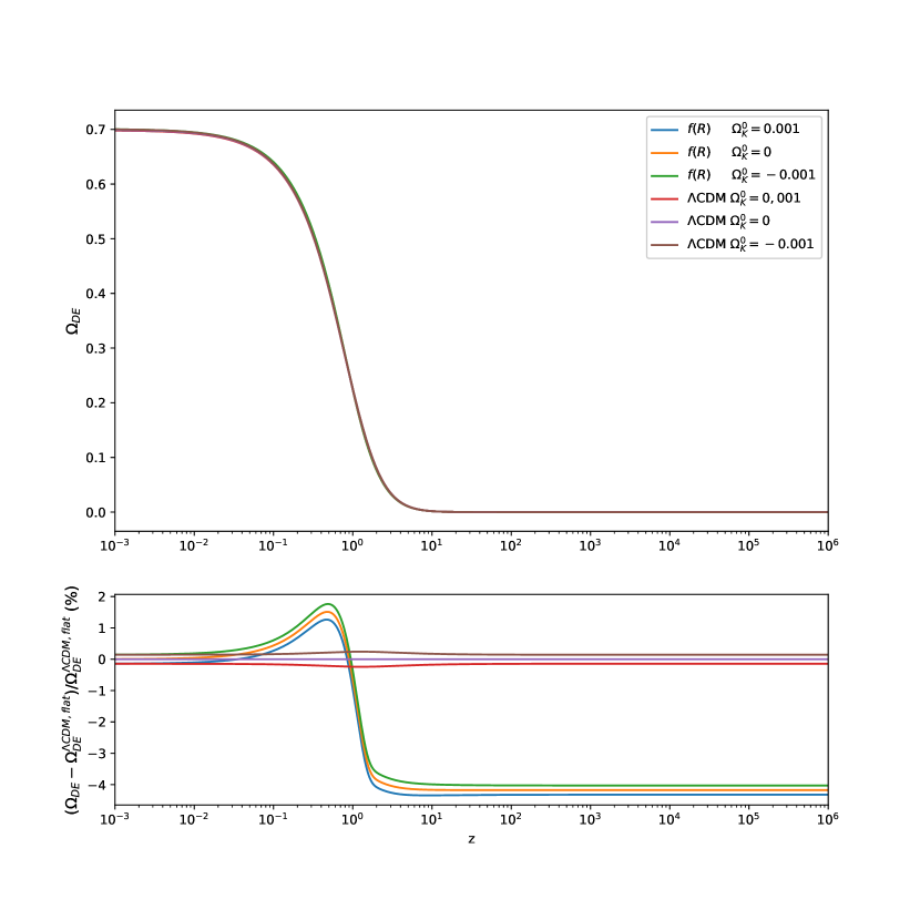
Figure 1: Evolutions of $\Omega_{DE}$ for exponential $f(R)$ gravity with $\lambda^{-1}=0.5$ and $\Lambda$CDM in open, flat and closed universe with $\Omega_{K}^{0}=(0.01,0,-0,01)$ (upper panel), and the residues with respect to flat $\Lambda$CDM $(\Omega_{DE}-\Omega_{DE}^{\Lambda CDM,flat})/\Omega_{DE}^{\Lambda CDM,flat}$ (lower panel), where the initial values are give by ($\Omega_{m}^{0}$, $\Omega_{r}^{0}$) = $(0.2998,1.5\times 10^{-3})$, $\Omega_{K}^{0}=(0.001,0,-0.001)$ and $H_{0}=67km/s/Mpc$.

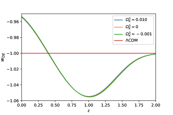
Figure 2: Evolutions of $w_{DE}$ for Exponential $f(R)$ gravity with $\lambda^{-1}=0.5$ and $\Omega_{K}^{0}=(0.01,0,-0,01)$ and $\Lambda$CDM, where the initial values are described in Fig. 1.

III.2 Global fitting

In this subsection, we present constraints on the cosmological parameters in the exponential $f(R)$ model without the spatial flatness assumption . With the modifications of CAMB at the background level and the CosmoMC package, we perform the MCMC analysis.

To break the geometrical degeneracy Efstathiou:1998xx ; Howlett:2012mh , we fit the model with the combinations of the observational data, including CMB temperature and polarization angular power spectra from Planck 2018 with high-$l$ TT, TE, EE , low-$l$ TT, EE, CMB lensing from SMICA Planck:2018vyg ; Planck:2018lbu ; Planck:2019kim ; Planck:2019nip , BAO observations from 6-degree Field Galaxy Survey (6dF) Beutler:2011gb , SDSS DR7 Main Galaxy Sample (MGS) Ross:2014qpa and BOSS Data Release 12 (DR12) BOSS:2016wmc , and supernova (SN) data from the Pantheon compilation Pan-STARRS1:2017jku . As we set the density parameter of curvature and the neutrino mass sum to be free, our fitting for the exponential $f(R)$ model contains nine free parameters, where the priors are listed in Table 1.

To find the best-fit results, we minimize the $\chi^{2}$ function, which is given by

$$\chi^{2}=\chi_{CMB}^{2}+\chi_{BAO}^{2}+\chi_{Pan}^{2}\,.$$ (32)

Explicitly, we take

$$\chi_{CMB}^{2}=\sum_{ll^{\prime}}(C^{obs}_{l}-C^{th}_{l})\mathcal{M}^{-1}_{ll^{\prime}}(C^{obs}_{l^{\prime}}-C^{th}_{l^{\prime}})$$ (33)

where $C^{obs(th)}_{l}$ corresponds to the observational (theoretical) value of the related power spectrum, and $\mathcal{M}$ is the covariance matrix for the CMB data Planck:2018vyg ; Planck:2018lbu .

For the BAO data, we adopt the dataset from 6-degree Field Galaxy Survey (6dF) at $z_{eff}=0.106$ Beutler:2011gb , SDSS DR7 Main Galaxy Sample (MGS) at $z_{eff}=0.15$ Ross:2014qpa and BOSS Data Release 12 (DR12) at $z_{eff}=(0.38,0.51,0.61)$  BOSS:2016wmc . As a result, we have

$$\chi_{BAO}^{2}=\chi_{6dF}^{2}+\chi_{MGS}^{2}+\chi_{DR12}^{2}.$$ (34)

For the uncorrelated data points, such as 6dF and MGS, $\chi^{2}$ is given by

$$\chi^{2}(p)=\sum^{N}_{i=1}\frac{[A_{th}(z_{i})-A_{obs}(z_{i})]^{2}}{\sigma^{2}_{i}},$$ (35)

where $A_{th}(z_{i})$ is the predicted value computed in the model under consideration, and $A_{obs}(z_{i})$ denotes the measured value at $z_{i}$ with the standard deviation $\sigma_{i}$. Note that in our study, we adopted 6dF and MGS, whose standard deviations are given by $\sigma_{6dF}=0.015$ and $\sigma_{MGS}=0.168$, respectively. The data points from DR12 are correlated. In this case, $\chi^{2}$ is given by

$$\chi_{DR12}^{2}=\bigg{[}\textbf{A}_{th}-\textbf{A}_{obs}\bigg{]}^{T}\cdot\textbf{C}^{-1}\cdot\bigg{[}\textbf{A}_{th}-\textbf{A}_{obs}\bigg{]},$$ (36)

where $\textbf{C}^{-1}$ is the inverse of the covariance matrix, which is an $6\times 6$ matrix given in Eq. (20) of Ref. Ryan:2019uor .

For the Pantheon SN Ia samples, there are 1048 data points scattering between $0.01\leq z\leq 2.3$, with the observable to be the distance modulus $\mu$ defined in Ref. Pan-STARRS1:2017jku . We have that

$$\chi_{Pan}^{2}=\bigg{[}\bm{\mu}_{obs}-\bm{\mu}_{th}\bigg{]}^{T}\cdot\textbf{Cov}^{-1}\cdot\bigg{[}\bm{\mu}_{obs}-\bm{\mu}_{th}\bigg{]},$$ (37)

where $\textbf{Cov}^{-1}$ is the inverse covariance matrix Pan-STARRS1:2017jku of the sample including the contributions from both the statistical and systematic errors. The covariance matrix of Pantheon samples can also be found in the website .

Table 1: This table contains priors of cosmological parameters for exponential $f(R)$ and $\Lambda$CDM models.

Parameter	Prior
$f(R)$ model parameter $\lambda^{-1}$	$0.1\leq\lambda^{-1}\leq 1$
Curvature parameter $\Omega_{K}$	$-0.1\leq\Omega_{K}\leq 0.1$
Baryon density	$0.5\leq 100\Omega_{b}h^{2}\leq 10$
CDM density	$0.1\leq 100\Omega_{c}h^{2}\leq 99$
Optical depth	$0.01\leq\tau\leq 0.8$
Neutrino mass sum	$0\leq\Sigma m_{\nu}\leq 2$ eV
Angular size of the sound horizon	$0.5\leq 100\theta_{MC}\leq 10$
Scalar power spectrum amplitude	$1.61\leq\ln\left(10^{10}A_{s}\right)\leq 3.91$
Spectral index	$0.8\leq n_{s}\leq 1.2$

Table 2: The constraints of cosmological parameters for exponential $\Lambda$CDM models fitted with CMB+BAO+SN data sets, where the cosmological parameters are given at 95% C.L, while $\Lambda^{-1}$ and $\Sigma m_{\nu}$ are given at 68% C.L

Parameter	Exp $f(R)$	$\Lambda$CDM
$\Omega_{b}h^{2}$	$0.02241^{+0.00032}_{-0.00031}$	$0.02242^{+0.00031}_{-0.00031}$
$\Omega_{c}h^{2}$	$0.11954^{+0.00270}_{-0.00266}$	$0.11948^{+0.00268}_{-0.00263}$
$\tau$	$0.05537^{+0.01518}_{-0.01424}$	$0.05558^{+0.01567}_{-0.01407}$
$\Omega_{K}$	$0.00050^{+0.00420}_{-0.00414}$	$0.00050^{+0.00400}_{-0.00403}$
$\Sigma m_{\nu}[eV]$	$<0.06816$	$<0.06121$
$\lambda^{-1}$	$<0.42927^{+0.39921}_{-0.32927}$	$-$
$H_{0}(km/s/Mpc)$	$67.73344^{+1.39013}_{-1.45947}$	$67.95862^{+1.23489}_{-1.22664}$
${\rm{Age}}/{\rm{Gyr}}$	$13.7550^{+0.1585}_{-0.1581}$	$13.76^{+0.1578}_{-0.1514}$
$\chi^{2}_{best-fit}$	$3821.50$	$3821.84$

Table 3: The results of AIC, BIC and DIC computed from the sample we use for both $\Lambda$CDM and exponential $f(R)$ models, where $\Delta AIC=AIC_{f(R)}-AIC_{\Lambda CDM}$, $\Delta BIC=BIC_{f(R)}-BIC_{\Lambda CDM}$, and $\Delta DIC=DIC_{f(R)}-DIC_{\Lambda CDM}$.

Model	$\chi^{2}_{min}$	AIC	$\Delta$AIC	BIC	$\Delta$BIC	DIC	$\Delta$DIC
$\Lambda$CDM	$3821.84$	$3837.84$	$0$	$3887.35$	$0$	$3850.38$	$0$
Exp $f(R)$	$3821.50$	$3839.50$	$1.66$	$3895.20$	$7.85$	$3851.87$	$1.49$

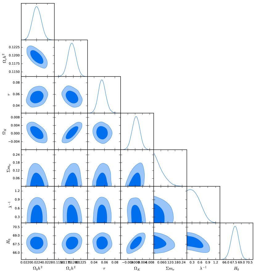
Figure 3: Marginalized one and two-dimensional constraints of $\Omega_{b}h^{2}$, $\Omega_{c}h^{2}$, $\tau$, $\Omega_{K}$, $\sum m_{\nu}$, $\lambda^{-1}$ and $H_{0}$ for exponential $f(R)$ with the combined data of CMB+BAO+SN, where the contour lines represent 68$\%$  and 95$\%$  C.L., respectively.

The global fitting results of the exponential $f(R)$ model without the spatial flatness assumption with CMB+BAO+SN data sets are shown in Fig. 3 and listed in Table 2. We note that the exponential $f(R)$ model is barely distinguishable from $\Lambda$CDM. This statement is in agreement with the previous work in the flat universe Geng:2014yoa . FromTable 2, we see that the model and curvature density parameters are constrained to be $\lambda^{-1}=0.42927^{+0.39921}_{-0.32927}$ at 68$\%$ C.L and $\Omega_{K}=-0.00050^{+0.00420}_{-0.00414}$ at 95$\%$ C.L for the exponential $f(R)$ model, respectively. Note that the flat $\Lambda$CDM model is recovered when $\lambda^{-1}=0$ and $\Omega_{K}=0$. We also obtain that $\chi^{2}=3821.50~{}(3821.84)$ for $f(R)$ ($\Lambda$CDM) with $\chi^{2}_{f(R)}\lesssim\chi^{2}_{\Lambda CDM}$, indicating that exponential $f(R)$ is consistent with $\Lambda$CDM. The neutrino mass sum is evaluated to be $\Sigma m_{\nu}<0.06816~{}(0.06121)$ for $f(R)$ ($\Lambda$CDM) at 68$\%$ C.L., which is relaxed at 11 $\%$ comparing with $\Lambda$CDM. This phenomenon is caused by the shortened age of the universe in the exponential $f(R)$ model, in which the matter density fluctuation is suppressed as discussed in Chen:2019uci and Sec. III.1.

To compare exponential $f(R)$ gravity with $\Lambda$CDM, we introduce the Akaike Information Criterion (AIC) Akaike:1974 , Bayesian Information Criterion (BIC) Schwarz:1978tpv , and Deviance Information Criterion (DIC) Spiegelhalter:2002yvw . The AIC is defined through the maximum likelihood $\mathcal{L}_{max}$ (satisfying $-2\,{\rm ln}\,{\mathcal{L}}_{max}\propto\chi^{2}_{min}$ under the Gaussian likelihood assumption) and the number of model parameters, $d$:

$$AIC=-2\,{\rm ln}\,{\mathcal{L}}_{max}+2d=\chi^{2}_{min}+2d.$$ (38)

The BIC is defined as

$$BIC=-2\,{\rm ln}\,{\mathcal{L}}_{max}+d{\rm ln}N=\chi^{2}_{min}+d{\rm ln}N,$$ (39)

where $N$ is the number of data points.

The DIC is determined by the quantities obtained from posterior distributions, given by

$$DIC=D(\bar{\theta})+2\,p_{D},$$ (40)

where $D(\theta)=-2\,{\rm ln}\,{\mathcal{L}}(\theta)+C,p_{D}=\overline{D(\theta)}-D(\overline{\theta}),C$ is a constant, and $p_{D}$ represents the effective number of parameters in the model.

We now compute the AIC, BIC, and DIC values from CMB+BAO+SN samples described above for both models, with the difference given by $\Delta AIC=AIC_{f(R)}-AIC_{\Lambda CDM}=1.66$, $\Delta BIC=BIC_{f(R)}-BIC_{\Lambda CDM}=7.85$, and $\Delta DIC=DIC_{f(R)}-DIC_{\Lambda CDM}=1.49$, respectively. The results are summarized in Table 3, where the differences are residuals with respect to the $\Lambda$CDM model. Since $\Delta AIC,\,\Delta DIC)<2$, being small, there is no strong preference between the exponential $f(R)$ and $\Lambda$CDM models in terms of AIC and DIC Rezaei:2021qpq . However, as $6<\Delta BIC<10$, there is a strong evidence against the exponential $f(R)$ model Liddle:2007fy .

IV Conclusions

We have considered the exponential $f(R)$ gravity model without the spatial flatness assumption. We have derived the energy density ($\rho_{de}$) and pressure ($p_{de}$) of dark energy, and simplified the modified Friedmann equations into a second order differential equation in Eqs. (24)-(27) with the involvement of the spatial curvature $K$. In our numerical calculations, by modifying the CAMB program for the exponential $f(R)$ model in open, flat and closed universe, we have studied the cosmological evolutions of the dark energy density parameter and equation of state. We have found that exponential $f(R)$ has a shortened age of the universe comparing with $\Lambda$CDM. To constrain the cosmological parameters of the exponential $f(R)$ model, we have used the CosmoMC package to explore the parameter space. In particular, we have obtained that $\lambda^{-1}=0.42927^{+0.39921}_{-0.32927}$ at 68$\%$ C.L and $\Omega_{K}=-0.00050^{+0.00420}_{-0.00414}$ at 95$\%$ C.L. In addition, we have gotten that $\chi^{2}=3821.50~{}(3821.84)$ for $f(R)$ ($\Lambda$CDM) with $\chi^{2}_{f(R)}\lesssim\chi^{2}_{\Lambda CDM}$, which matches the previous work in the flat universe Yang:2010xq .

We have also evaluated the AIC, BIC, and DIC values for the exponential $f(R)$ and $\Lambda$CDM models. We have shown that the $\Lambda$CDM model is slightly more preferable in terms of BIC, but such a preference has not been found based on the AIC and DIC results. We note that all values of AIC, BIC and DIC in $f(R)$ are smaller than those in $\Lambda$CDM in our study, whereas it is not the case in some models discussed in the literature, such as those in Refs. Zheng:2021uee ; Rezaei:2021qpq ; Liddle:2007fy . It is known that different combinations of the data may draw to different conclusions due to the dimensional inconsistency Liddle:2007fy . Clearly, to compare models in cosmology, it is necessary to explore various probes along with different data sets.

References

- (1) A. G. Riess et al. [Supernova Search Team], Astron. J. 116, 1009-1038 (1998)
- (2) S. Perlmutter et al. [Supernova Cosmology Project], Astrophys. J. 517, 565-586 (1999)
- (3) S. Weinberg, Rev. Mod. Phys. 61, 1-23 (1989)
- (4) P. J. E. Peebles and B. Ratra, Rev. Mod. Phys. 75, 559-606 (2003)
- (5) A. G. Riess, S. Casertano, W. Yuan, L. M. Macri and D. Scolnic, Astrophys. J. 876, no.1, 85 (2019)
- (6) E. J. Copeland, M. Sami and S. Tsujikawa, Int. J. Mod. Phys. D 15, 1753-1936 (2006)
- (7) M. Li, X. D. Li, S. Wang and Y. Wang, Commun. Theor. Phys. 56, 525-604 (2011)
- (8) S. Nojiri and S. D. Odintsov, Phys. Rept. 505, 59-144 (2011)
- (9) T. P. Sotiriou and V. Faraoni, Rev. Mod. Phys. 82, 451-497 (2010)
- (10) A. De Felice and S. Tsujikawa, Living Rev. Rel. 13, 3 (2010)
- (11) K. Bamba, C. Q. Geng and C. C. Lee, JCAP 11, 001 (2010)
- (12) A. A. Starobinsky, JETP Lett. 86, 157-163 (2007)
- (13) W. Hu and I. Sawicki, Phys. Rev. D 76, 064004 (2007)
- (14) S. Tsujikawa, Phys. Rev. D 77, 023507 (2008)
- (15) J. Y. Cen, S. Y. Chien, C. Q. Geng and C. C. Lee, Phys. Dark Univ. 26, 100375 (2019)
- (16) E. V. Linder, Phys. Rev. D 80, 123528 (2009)
- (17) K. Bamba, C. Q. Geng and C. C. Lee, JCAP 08, 021 (2010)
- (18) E. Di Valentino, A. Melchiorri and J. Silk, Nature Astron. 4, no.2, 196-203 (2019)
- (19) P. Zhang, Phys. Rev. D 73, 123504 (2006)
- (20) L. Yang, C. C. Lee, L. W. Luo and C. Q. Geng, Phys. Rev. D 82, 103515 (2010)
- (21) A. Lewis, A. Challinor and A. Lasenby, Astrophys. J. 538, 473-476 (2000)
- (22) A. Lewis and S. Bridle, Phys. Rev. D 66, 103511 (2002)
- (23) Y. C. Chen, C. Q. Geng, C. C. Lee and H. Yu, Eur. Phys. J. C 79, no.2, 93 (2019)
- (24) S. Vagnozzi, E. Di Valentino, S. Gariazzo, A. Melchiorri, O. Mena and J. Silk, Phys. Dark Univ. 33, 100851 (2021) doi:10.1016/j.dark.2021.100851 [arXiv:2010.02230 [astro-ph.CO]].
- (25) G. Efstathiou and J. R. Bond, Mon. Not. Roy. Astron. Soc. 304, 75-97 (1999)
- (26) C. Howlett, A. Lewis, A. Hall and A. Challinor, JCAP 04, 027 (2012)
- (27) N. Aghanim et al. [Planck], Astron. Astrophys. 641, A6 (2020) [erratum: Astron. Astrophys. 652, C4 (2021)]
- (28) N. Aghanim et al. [Planck], Astron. Astrophys. 641, A8 (2020)
- (29) Y. Akrami et al. [Planck], Astron. Astrophys. 641, A9 (2020)
- (30) N. Aghanim et al. [Planck], Astron. Astrophys. 641, A5 (2020)
- (31) Beutler, Florian, et al. Monthly Notices of the Royal Astronomical Society 416.4, 3017-3032 (2011)
- (32) A. J. Ross, L. Samushia, C. Howlett, W. J. Percival, A. Burden and M. Manera, Mon. Not. Roy. Astron. Soc. 449, no.1, 835-847 (2015)
- (33) S. Alam et al. [BOSS], Mon. Not. Roy. Astron. Soc. 470, no.3, 2617-2652 (2017)
- (34) J. Ryan, Y. Chen and B. Ratra, Mon. Not. Roy. Astron. Soc. 488, no.3, 3844-3856 (2019)
- (35) D. M. Scolnic et al. [Pan-STARRS1], Astrophys. J. 859, no.2, 101 (2018)
- (36) C. Q. Geng, C. C. Lee and J. L. Shen, Phys. Lett. B 740, 285-290 (2015)
- (37) Akaike, H., IEEE Transactions on Automatic Control, vol. 19, pp. 716–723, 1974.
- (38) G. Schwarz, Annals Statist. 6, 461-464 (1978)
- (39) D. J. Spiegelhalter, N. G. Best, B. P. Carlin and A. van der Linde, J. Roy. Statist. Soc. B 64, no.4, 583-639 (2002)
- (40) M. Rezaei and M. Malekjani, Eur. Phys. J. Plus 136, no.2, 219 (2021)
- (41) A. R. Liddle, Mon. Not. Roy. Astron. Soc. 377, L74-L78 (2007)
- (42) J. Zheng, Y. Chen, T. Xu and Z. H. Zhu, [arXiv:2107.08916 [astro-ph.CO]].