Causal Modeling With Infinitely Many Variables

Abstract

Structural-equations models (SEMs) are perhaps the most commonly used framework for modeling causality. However, as we show, naively extending this framework to infinitely many variables, which is necessary, for example, to model dynamical systems, runs into several problems. We introduce GSEMs (generalized SEMs), a flexible generalization of SEMs that directly specify the results of interventions, in which (1) systems of differential equations can be represented in a natural and intuitive manner, (2) certain natural situations, which cannot be represented by SEMs at all, can be represented easily, (3) the definition of actual causality in SEMs carries over essentially without change.

1 Introduction

For scientists trying to understand causal relationships, and policymakers grappling with the consequences of their decisions, the structure of causality itself is of great importance. One influential paradigm for formalizing causality, structural-equations models (SEMs), describes causal relationships as a collection of structural equations. Actions taken by a scientist or policymaker (interventions) manifest as modifications to the structural equations; for example, if $X$ represents the rental price of an apartment, imposing rent control amounts to replacing the equation for $X$ with $X=r$, producing a new SEM.

SEMs are well studied; there are standard techniques for reasoning about the outcomes of given interventions. For example, SEMs without cyclic dependencies have a unique outcome for any given intervention, which can be obtained simply by solving the equations in any order consistent with the dependencies between variables. However, this property does not hold when there are infinitely many variables. Consider the simple SEM with binary variables $X_{1},X_{2},\dots$, where the equations are $X_{1}=X_{2},X_{2}=X_{3},\dots$. Intuitively, this says that $X_{1}$ gets the value that $X_{2}$ has, $X_{2}$ gets the value that $X_{3}$ has, and so on. There are clearly no acyclic dependencies here; nevertheless, these equations have two solutions: $X_{i}=0$ for all $i$, and $X_{i}=1$ for all $i$. In this case the solutions are easy to determine, but in more complex examples, for example, a SEM with equations

$$X_{i}=\begin{cases}3X_{i+1}+1&X_{i+1}\text{ is odd}\\ X_{i+1}/2&X_{i+1}\text{ is even,}\\ \end{cases}$$

it may be extremely difficult to determine the outcomes of interventions. The problem here is that the dependency relation is not well founded: $X_{1}$ depends on $X_{2}$, which depends on $X_{3}$, and so on. (A relation $\succ$ is well-founded if and only if there are no infinite descending sequences $X_{1}\succ X_{2}\succ X_{3}\succ\dots$.) The lack of well-foundedness is the source of the problem; it is easy to show that if the dependency relation is well-founded, then there will be a unique outcome.

Unfortunately, the problem of ill-founded dependencies is unavoidable when working with dynamical systems. Suppose that we were to try to represent a dynamical system using a SEM. Perhaps the most natural approach would have variables $X_{t}$ representing the state of a dynamical system at time $t$, where $t$ ranges over an interval of real numbers. In general, we expect that changing the value of $X_{s}$ will affect the value of $X_{t}$ for all $t>s$. That is, the dependency relation can be identified with the less-than relation on the real numbers, which is not well founded.

We might try to avoid this problem by choosing a finite timestep $\epsilon>0$, and considering what happens only at time steps that are multiples of $\epsilon$, using structural equations of the form $X_{t+\epsilon}=f(X_{t},Y_{t})$. This idea is reasonable and similar to practical finite-difference methods for finding numerical solutions to dynamical systems. But it has several problems. Most importantly, the modeler must design new approximate structural equations for each new dynamical system and argue that these are reasonable for the application at hand. The approach also inherits issues from numerical computing that are best kept separate from causal modeling issues to the extent possible. These issues include the need to choose $\epsilon$ (which depends on the particular system under study and the questions of interest) and validate that the results are independent of this choice.

To capture dynamical systems, we propose a more flexible class of models that we call generalized structural-equations models (GSEMs). It is easy to show that GSEMs indeed generalize SEMs (see Theorem 3.1). Given a SEM and an intervention, we can produce a new SEM that represents the result of the intervention by modifying the relevant equations. GSEMs represent the same input-output relationships as SEMs—a GSEM and an allowed intervention maps to a new GSEM, while a GSEM and a context together determine a set of possible outcomes (assignments to the endogenous variables)—without committing to a specific mechanism for producing the outcomes. Indeed, any mapping from interventions and contexts to outcomes (all defined with respect to some set of variables) is a GSEM. In this sense, GSEMs are the most general causal model that has the same “interface” or input-output behavior as SEMs. In fact, even if we restrict to settings with only finitely many variables, GSEMs are more expressive than SEMs; see Example 3.6.

Due to their generality, GSEMs no longer have some of the most appealing features of SEMs. Most importantly, GSEMs cannot be described using directed acyclic graphs, as SEMs can. Thus, many of the graphical tools developed for analyzing SEMs (such as the do-calculus) do not apply to GSEMs. However, we feel that this loss is worth accepting, for two reasons. First, it is worth understanding what tools remain to causal analysts when the graphical structure of SEMs is removed. Second, and more significantly, we show that (unlike SEMs), GSEMs can capture many standard formalisms for representing causality in infinitary settings, including dynamical systems, hybrid automata Alur et al. (1992) (a popular formalism for describing mixed discrete-continuous systems), and the rule-based models commonly used in molecular biology and organic chemistry (see Laurent et al. (2018) and the references therein). In particular, dynamical systems can be represented in a direct and natural way using GSEMs, avoiding all the problems mentioned above. The definition (see Section 4) is nothing more than the textbook definition of the solution of a system of differential equations.

Thus, GSEMs serve as a unifying framework for many disparate models of causality. Moreover, because GSEMs have the same interface as SEMs, any definition depending only on inputs and outputs (interventions and their outcomes) can be immediately applied to GSEMs. In particular, the notion of actual causality (whether event $X$ caused event $Y$ in some concrete situation) given by Halpern and Pearl [2005] and later modified by Halpern [2015; 2016] can be applied to GSEMs almost without modification (see Section 6). This means that causal modelers from, say, environmental scientists studying predator-prey dynamical systems to molecular biologists studying chemical reaction pathways, can use the same language of definitions to describe actual causality and related notions.

These problems can also be handled by causal constraints models (CCMs) Blom et al. (2019), which were introduced to get around some of the restrictions of SEMs when modeling equilibrium solutions of dynamical systems. GSEMs and CCMs are actually equally expressive (Theorem 5.1). However, the definition of GSEMs is much simpler than the definition of CCMs. Moreover, since GSEMs are a more straightforward generalization of SEMs than CCMs, they are arguably easier to use for those familiar with SEMs (as evidenced by the ease with which we carry over the definition of actual causality).

The rest of the paper is organized as follows. In Section 2, we review the standard SEM framework. In Section 3, we formally define GSEMs, relate them to SEMs, and describe some of their advantages in more detail. In Section 4, we show how to use GSEMs to model trajectories of dynamical systems. In Section 5, we consider three other classes of models: causal constraints models, hybrid automata, and rule-based models. We show how GSEMs are a reformulation of causal constraints models, how they can be used to answer causal questions about hybrid automata, and how they complement existing ad hoc causal modeling techniques defined for rule-based models.

2 SEMs: a review

Formally, a structural-equations model $M$ is a pair $({\cal S},{\cal F})$, where ${\cal S}$ is a signature, which explicitly lists the endogenous and exogenous variables and characterizes their possible values, and ${\cal F}$ defines a set of modifiable structural equations, relating the values of the variables. We extend the signature to include a set of allowed interventions, as was done in earlier work Beckers and Halpern (2019); Rubenstein et al. (2017).

Intuitively, allowed interventions are the ones that are feasible or meaningful. A signature ${\cal S}$ is a tuple $({\cal U},{\cal V},{\cal R},{\cal I})$. ${\cal U}$ is a set of exogenous variables, ${\cal V}$ is a set of endogenous variables, and ${\cal R}$ associates with every variable $Y\in{\cal U}\cup{\cal V}$ a nonempty, finite set ${\cal R}(Y)$ of possible values for $Y$ (i.e., the set of values over which $Y$ ranges). We assume (as is typical for SEMs) that ${\cal U}$ and ${\cal V}$ are finite sets, and adopt the convention that for $\mathaccent 382{Y}\subseteq{\cal U}\cup{\cal V}$, ${\cal R}(\mathaccent 382{Y})$ denotes the product of the ranges of the variables appearing in $\mathaccent 382{Y}$; that is, ${\cal R}(\mathaccent 382{Y})\coloneqq\times_{Y\in\mathaccent 382{Y}}{\cal R}(Y)$. Finally, an intervention $I\in{\cal I}$ is a set of pairs $(X,x)$, where $X\in{\cal V}$ and $x\in{\cal R}(X)$. For each $X\in{\cal V}$, there is at most one $x\in{\cal R}(X)$ with $(X,x)\in I$. We abbreviate an intervention $I$ by $\mathaccent 382{X}\leftarrow\mathaccent 382{x}$, where $\mathaccent 382{X}\subseteq{\cal V}$ and, unless $\mathaccent 382{X}$ is empty, $\mathaccent 382{x}\in{\cal R}(\mathaccent 382{X})$. Although this notation makes most sense if $\mathaccent 382{X}$ is nonempty, we allow $\mathaccent 382{X}$ to be empty (which amounts to not intervening at all). If $I$ consists of exactly one pair $(Y,y)$, we abbreviate $I$ as $Y\leftarrow y$.

${\cal F}$ associates with each endogenous variable $X\in{\cal V}$ a function denoted $F_{X}$ such that $F_{X}:{\cal R}({\cal U}\cup{\cal V}-\{X\})\rightarrow{\cal R}(X)$. This mathematical notation just makes precise the fact that $F_{X}$ determines the value of $X$, given the values of all the other variables in ${\cal U}\cup{\cal V}$. If there is one exogenous variable $U$ and three endogenous variables, $X$, $Y$, and $Z$, then $F_{X}$ defines the values of $X$ in terms of the values of $Y$, $Z$, and $U$. For example, we might have $F_{X}(u,y,z)=u+y$, which is usually written as $X=U+Y$. Thus, if $Y=3$ and $U=2$, then $X=5$, regardless of how $Z$ is set.

The structural equations define what happens in the presence of external interventions. Setting the value of some variable $X$ to $x$ in a SEM $M=({\cal S},{\cal F})$ results in a new SEM, denoted $M_{X\leftarrow x}$, which is identical to $M$, except that the equation for $X$ in ${\cal F}$ is replaced by $X=x$. Interventions on subsets $\mathaccent 382{X}$ of ${\cal V}$ are defined similarly. Notice that $M_{\mathaccent 382{X}\leftarrow\mathaccent 382{x}}$ is always well defined, even if $(\mathaccent 382{X}\leftarrow\mathaccent 382{x})\notin{\cal I}$. In earlier work, the reason that the model included allowed interventions was that, for example, relationships between two models were required to hold only for allowed interventions (i.e., the interventions that were meaningful). As we shall see, here, the fact that we do not have to specify what happens for certain interventions has a more significant impact.

Given a context ${\bf u}\in{\cal R}({\cal U})$, the outcomes of a SEM $M$ under intervention $\mathaccent 382{X}\leftarrow\mathaccent 382{x}$ are all assignments of values ${\bf v}\in{\cal R}({\cal V})$ such that the assignments ${\bf u}$ and ${\bf v}$ together satisfy the structural equations of $M_{\mathaccent 382{X}\leftarrow\mathaccent 382{x}}$. This set of outcomes is denoted $M({\bf u},\mathaccent 382{X}\leftarrow\mathaccent 382{x})$. Given an outcome ${\bf v}$, we denote by ${\bf v}[X]$ and ${\bf v}[\mathaccent 382{X}]$ the value that ${\bf v}$ assigns to $X$ and the restriction of ${\bf v}$ to ${\cal R}(\mathaccent 382{X})$ respectively. We also use this notation for interventions; for example, $\mathaccent 382{y}[X]$ is the value that intervention $\mathaccent 382{Y}\leftarrow\mathaccent 382{y}$ assigns to variable $X\in\mathaccent 382{Y}$.

As discussed in the introduction, an important special case of SEMs are acyclic (or recursive) SEMs. Formally, an acyclic SEM is one for which, for every context ${\bf u}\in{\cal R}(U)$, there is some total ordering $\prec_{\bf u}$ of the endogenous variables (the ones in ${\cal V}$) such that if $X\prec_{\bf u}Y$, then $X$ is independent of $Y$, that is, $F_{X}({\bf u},\ldots,y,\ldots)=F_{X}({\bf u},\ldots,y^{\prime},\ldots)$ for all $y,y^{\prime}\in{\cal R}(Y)$. Intuitively, if a theory is acyclic, there is no feedback. Acyclic models always have unique outcomes; this is a consequence of assuming that ${\cal V}$ is finite.

In order to talk about SEMs and the information they represent more precisely, we use the formal language ${\cal L}({\cal S})$ for SEMs having signature ${\cal S}$, introduced by Halpern [2000]; see also Galles and Pearl (1998). An informal description of this language follows; for more details, see Halpern (2000). We restrict the language used by Halpern [2000] to formulas that mention only allowed interventions. Fix a signature ${\cal S}=({\cal U},{\cal V},{\cal R},{\cal I})$. Given an assignment ${\bf v}\in{\cal R}({\cal V})$, the primitive event $X=x$ is true of ${\bf v}$, written ${\bf v}\models(X=x)$, if ${\bf v}[X]=x$; otherwise it is false. We extend this definition to events $\varphi$, which are Boolean combinations of primitive events, in the obvious way. Given a SEM $M$ with signature ${\cal S}$ and an allowed intervention $\mathaccent 382{Y}\leftarrow\mathaccent 382{y}\in{\cal I}$, the atomic causal formula $[\mathaccent 382{Y}\leftarrow\mathaccent 382{y}]\varphi$ is true in context ${\bf u}$, written $(M,{\bf u})\models[\mathaccent 382{Y}\leftarrow\mathaccent 382{y}]\varphi$ if, for all outcomes ${\bf v}\in M({\bf u},\mathaccent 382{Y}\leftarrow\mathaccent 382{y})$, we have ${\bf v}\models\varphi$. Again, we extend this definition to causal formulas, which are Boolean combinations of atomic formulas, in the obvious way. The language ${\cal L}({\cal S})$ consists of all causal formulas (over ${\cal S}$). Using these formulas, we can also talk about properties that only some of the outcomes ${\bf v}\in M({\bf u},\mathaccent 382{Y}\leftarrow\mathaccent 382{y})$ have. For an event $\varphi$, define $\langle\mathaccent 382{Y}\leftarrow\mathaccent 382{y}\rangle\varphi$ as $\neg[\mathaccent 382{Y}\leftarrow\mathaccent 382{y}](\neg\varphi)$. This formula is true exactly when $\varphi$ is true of at least one outcome ${\bf v}\in M({\bf u},\mathaccent 382{Y}\leftarrow\mathaccent 382{y})$.

The language of causal formulas completely characterizes the outcomes of a causal model with finite outcome sets, in the following precise sense. (For the purposes of this paper, a causal model is either a SEM, a GSEM, or a CCM.)

Theorem 2.1

: If $M$ and $M^{\prime}$ are causal models over the same signature ${\cal S}$ that, given a context and intervention, return a finite set of outcomes, then $M$ and $M^{\prime}$ have the same outcomes (that is, for all ${\bf u}\in{\cal R}({\cal U})$ and $I\in{\cal I}$, $M({\bf u},I)=M^{\prime}({\bf u},I)$) if and only if they satisfy the same set of causal formulas (that is, for all ${\bf u}\in{\cal R}({\cal U})$ and $\psi\in{\cal L}({\cal S})$, $M,{\bf u}\models\psi\Leftrightarrow M^{\prime},{\bf u}\models\psi$).

The proof of this and all other results not in the main text can be found in the appendix.

A short note on notation; consistent with the foregoing section, we use capital letters $X,Y$ to denote variables, lowercase letters $x,y$ to denote the corresponding values; letters with arrows $\mathaccent 382{X},\mathaccent 382{Y},\mathaccent 382{x},\mathaccent 382{y}$ to denote vectors of variables and their corresponding vectors of values. We use boldface ${\bf u}$ and ${\bf v}$ for contexts and outcomes, respectively. We use $M,M^{\prime}$ to denote causal models, script letters ${\cal S},{\cal U},{\cal V},{\cal R},{\cal I}$ to denote a model’s signature and its components, script ${\cal F}$ for a SEM’s structural equations, and boldface ${\bf F}$ for a GSEM’s outcomes mapping (see below).

3 Generalized structural-equations models

The main purpose of causal modeling is to reason about a system’s behavior under intervention. A SEM can be viewed as a function that takes a context ${\bf u}$ and an intervention $\mathaccent 382{Y}\leftarrow\mathaccent 382{y}$ and returns a set of outcomes, namely, the set of all solutions to the structural equations after replacing the equations for the variables in $\mathaccent 382{Y}$ with $\mathaccent 382{Y}=\mathaccent 382{y}$.

Viewed in this way, generalized structural-equations models (GSEMs) are a generalization of SEMs. In a GSEM, there is a function ${\bf F}$ that takes a context ${\bf u}$ and an intervention $\mathaccent 382{Y}\leftarrow\mathaccent 382{y}$ and returns a set of outcomes. However, the outcomes need not be determined by solving a set of suitably modified equations as they are for SEMs. This relaxation gives GSEMs the ability to concisely represent dynamical systems and other systems with infinitely many variables, and the flexibility to handle situations involving finitely many variables that cannot be modeled by SEMs.

Because GSEMs don’t have the structure that SEMs have by virtue of being defined in terms of structural equations, we may want to rule out certain unintuitive possibilities. In particular, we require that after intervening to set $\mathaccent 382{Y}\leftarrow\mathaccent 382{y}$, all outcomes satisfy $\mathaccent 382{Y}=\mathaccent 382{y}$.

3.1 GSEMs and SEMs

Formally, a generalized structural-equations model (GSEM) $M$ is a pair $({\cal S},{\bf F})$, where ${\cal S}$ is a signature, and ${\bf F}$ is a mapping from contexts and interventions to sets of outcomes. More precisely, a signature ${\cal S}$ is a quadruple $({\cal U},{\cal V},{\cal R},{\cal I})$ where, as before, ${\cal U}$ is a set of exogenous variables, ${\cal V}$ is a set of endogenous variables, and ${\cal R}$ associates with every variable $Y$ in ${\cal U}\cup{\cal V}$ a nonempty, finite set ${\cal R}(Y)$ of possible values for $Y$; we extend ${\cal R}$ to subsets of ${\cal V}$ in the same way as before. However, we no longer require that ${\cal U}$, ${\cal V}$ or the sets ${\cal R}(Y)$ for $Y\in{\cal U}\cup{\cal V}$ be finite. The mapping ${\bf F}$ is a function ${\bf F}:{\cal I}\times{\cal R}({\cal U})\to{\cal P}({\cal R}({\cal V}))$, where ${\cal P}$ denotes the powerset operation. That is, it maps a context ${\bf u}\in{\cal R}(U)$ and an allowed intervention $I\in{\cal I}$ to a set of outcomes ${\bf F}({\bf u},I)\in{\cal P}({\cal R}({\cal V}))$. As with SEMs, we denote these outcomes by $M({\bf u},I)$. As stated above, we require that outcomes ${\bf v}\in{\bf F}({\bf u},\mathaccent 382{X}\leftarrow\mathaccent 382{x})$ satisfy ${\bf v}[\mathaccent 382{X}]=\mathaccent 382{x}$. In the special case where all interventions are allowed, we take ${\cal I}={\cal I}_{univ}$, the set of all interventions. We note that, while these semantics are deterministic, we can bring probability back into the picture just as we do for SEMs: by putting a probability on contexts. To keep things simple, we consider only deterministic examples in the rest of the paper.

We now make precise the sense in which GSEMs generalize SEMs. Two causal models $M$ and $M^{\prime}$ are equivalent, denoted $M\equiv M^{\prime}$, if they have the same signature and they have the same outcomes, that is, if for all sets of variables $\mathaccent 382{X}\subseteq{\cal V}$, all values $\mathaccent 382{x}\in{\cal R}(\mathaccent 382{X})$ such that $\mathaccent 382{X}\leftarrow\mathaccent 382{x}\in{\cal I}$, and all contexts ${\bf u}\in{\cal R}({\cal U})$, we have $M({\bf u},\mathaccent 382{X}\leftarrow\mathaccent 382{x})=M^{\prime}({\bf u},\mathaccent 382{X}\leftarrow\mathaccent 382{x})$.

Theorem 3.1

: For all SEMs $M$, there is a GSEM $M^{\prime}$ such that $M\equiv M^{\prime}$.

Just as for SEMs, the intervention $I=\mathaccent 382{Y}\leftarrow\mathaccent 382{y}$ on a GSEM $M$ induces another GSEM $M_{I}$. To define $M_{I}$ precisely, we must first define the composition of interventions.

Given interventions $\mathaccent 382{X}\leftarrow\mathaccent 382{x}$ and $\mathaccent 382{Y}\leftarrow\mathaccent 382{y}$, let their composition $I=\mathaccent 382{X}\leftarrow\mathaccent 382{x};\mathaccent 382{Y}\leftarrow\mathaccent 382{y}$ be the intervention that results by letting the intervention performed second ($\mathaccent 382{Y}\leftarrow\mathaccent 382{y}$) override the first on variables that both interventions affect; that is, $I=\mathaccent 382{X}\cup\mathaccent 382{Y}\leftarrow\mathaccent 382{z}$, where for $Z\in\mathaccent 382{X}\cup\mathaccent 382{Y}$,

$$\mathaccent 382{z}[Z]=\begin{cases}\mathaccent 382{y}[Z]\quad\mbox{if $Z\in\mathaccent 382{Y}$,}\\ \mathaccent 382{x}[Z]\quad\mbox{if $Z\in\mathaccent 382{X}-\mathaccent 382{Y}$.}\end{cases}$$

Given a GSEM $M=({\cal S},{\bf F},{\cal I})$ and an intervention $I\in{\cal I}$, define the intervened model $M_{I}$ to be $({\cal S},{\bf F}^{\prime},{\cal J})$, where ${\cal J}=\{J\in{\cal I}_{univ}:I;J\in{\cal I}\}$ and, for $J\in{\cal J}$, ${\bf F}^{\prime}({\bf u},J)={\bf F}({\bf u},I;J).$ (The same relationship holds between the signatures ${\cal I}$ of $M$ and ${\cal J}$ of $M_{I}$ when $M$ is a SEM.) Notice that if the set ${\cal I}$ is closed under composition, that is, if for all $I,J\in{\cal I}$ we have $I;J\in{\cal I}$, then ${\cal J}=\{J\in{\cal I}_{univ}:I;J\in{\cal I}\}\supseteq{\cal I}$, so that with $M_{I}$ we have all the interventions that we had with $M$, and perhaps more.

The skeptical reader may wonder if the mechanism of equation modification in SEMs really is doing the same thing as the mechanism of intervention composition in GSEMs. This is indeed the case. There are two equivalent ways to see this. The first is to show that equation modification and intervention composition are the same for SEMs.

Theorem 3.2

: For all SEMs $M$ and interventions $I,J\in{\cal I}$ such that $I;J\in{\cal I}$, we have that $M_{I}({\bf u},J)=M({\bf u},I;J)$.

The second is to show that interventions respect equivalences that hold between SEMs and GSEMs.

Theorem 3.3

: If $M$ and $M^{\prime}$ are causal models with $M\equiv M^{\prime}$, then for all $I\in{\cal I}$, we have that $M_{I}\equiv M^{\prime}_{I}$.

3.2 Finite GSEMs

GSEMs clearly differ from SEMs in that the sets of endogenous and exogenous variables and the range of each individual variable can be infinite. Consider the class of GSEMs where these restrictions are retained, which we call finite GSEMs. How do finite GSEMs relate to SEMs? Halpern [2000] showed that all SEMs satisfy an axiom system called $AX^{+}$(see Appendix A for more details). For example, one axiom (effectiveness) states that after setting $X\leftarrow x$, all outcomes have $X=x$: $[\mathaccent 382{W}\leftarrow\mathaccent 382{w};X\leftarrow x](X=x)$. While we imposed this constraint explicitly on GSEMs (and hence this axiom is valid in GSEMs—it is true in all contexts of all GSEMs), in SEMs there is no need to impose it; it is a property of the way outcomes are calculated. However, there are additional axioms, for example, one that requires unique outcomes if we intervene on all but one endogenous variable, that finite GSEMs do not satisfy. If we impose these axioms on finite GSEMs, we recover SEMs.

Theorem 3.4

: For all finite GSEMs over a signature ${\cal S}$ such that ${\cal I}={\cal I}_{univ}$ in which all the axioms of $AX^{+}$ are valid, there is an equivalent SEM, and vice versa.

Likewise, all acyclic SEMs satisfy an axiom system called $AX^{+}_{rec}$ (also described in Appendix A), which consists of the axioms in $AX^{+}$ along with two additional conditions. Imposing these axioms on finite GSEMs when all interventions are allowed recovers exactly the class of acyclic SEMs.

Theorem 3.5

: For all finite GSEMs over a signature ${\cal S}$ such that ${\cal I}={\cal I}_{univ}$ and all the axioms $AX^{+}_{rec}$ are valid, there is an equivalent acyclic SEM, and vice versa.

We remark that the axiom system $AX^{+}$ can be generalized so as to deal with arbitrary (not necessarily finite) GSEMs, and soundness and completeness results for GSEMs can be proved. We defer these results to a companion paper Peters and Halpern (2021).

Theorems 3.4 and 3.5 show that finite GSEMs satisfying $AX^{+}$ and $AX^{+}_{rec}$, respectively, are equivalent to SEMs and acyclic SEMs, respectively, if all interventions are allowed. This equivalence breaks down once we restrict the set of interventions; GSEMs are then strictly more expressive than SEMs, as the following example shows.

Example 3.6

: Suppose that Suzy is playing a shell game with two shells. One of the shells conceals a dollar; the other shell is empty. Suzy can choose to flip over a shell. If she does, the house flips over the other shell. If Suzy picks shell 1, which hides the dollar, she wins the dollar; otherwise she wins nothing. This example can be modeled by a GSEM $M_{shell}$ with two binary endogenous variables $S_{1},S_{2}$ describing whether shell 1 is flipped over and shell 2 is flipped over, respectively, and a binary endogenous variable $Z$ describing the change in Suzy’s winnings. (The GSEM also has a trivial exogenous variable whose range has size 1, so that there is only one context ${\bf u}$.) That defines ${\cal U},{\cal V}$, and ${\cal R}$; we set ${\cal I}=\{S_{1}\leftarrow 1,{\cal S}_{2}\leftarrow 1\}$; and ${\bf F}$ is defined as follows:

$${\bf F}({\bf u},S_{1}\leftarrow 1) =M_{shell}({\bf u},S_{1}\leftarrow 1)$$

$$=\{(S_{1}=1,S_{2}=1,Z=1)\}$$

$${\bf F}({\bf u},S_{2}\leftarrow 1) =M_{shell}({\bf u},S_{2}\leftarrow 1)$$

$$=\{(S_{1}=1,S_{2}=1,Z=0)\}.$$

$M_{shell}$ is clearly a valid GSEM. Furthermore, checking that $M_{shell}$ satisfies all the axioms in $AX^{+}$ is straightforward; see Appendix B (Theorem B.2) for details. However, no SEM $M^{\prime}$ with the same signature can have the outcomes $M^{\prime}({\bf u},S_{1}\leftarrow 1)=\{(S_{1}=1,S_{2}=1,Z=1)\}$ and $M^{\prime}({\bf u},S_{1}\leftarrow 2)=\{(S_{1}=1,S_{2}=1,Z=0)\}$. This is because in a SEM, the value of $Z$ would be specified by a structural equation $Z={\cal F}_{Z}({\cal U},S_{1},S_{2})$. This cannot be the case here, since there are two outcomes having $S_{1}=S_{2}=1$, but with different values of $Z$.  

This example shows that finite GSEMs (even restricted to those satisfying the axioms of $AX^{+}$) are more expressive than SEMs when not all interventions are allowed. The fundamental issue here is that $Z$ is determined by the intervention (which shell Suzy picks), not the state of the shells. In SEMs, the system’s behavior cannot depend explicitly on the intervention, only on the variables altered by the intervention. We note that Suzy’s situation can be modeled by a SEM with an additional variable describing Suzy’s action. (More precisely, one where the only allowed interventions set this variable’s value to match Suzy’s action.) However, this variable is redundant in the sense that Suzy’s action is already described by the intervention. Thus, arguably, the GSEM model is more natural.

4 Ordinary differential equations

In this section, we show how GSEMs can be used to model dynamical systems characterized by a system of ordinary differential equations (ODEs). Suppose that we have a system of ODEs of the form

$$\dot{\mathcal{X}}_{1} =F_{1}(\mathcal{X}_{1},\mathcal{X}_{2},\dots,\mathcal{X}_{n})$$

$$\dot{\mathcal{X}}_{2} =F_{2}(\mathcal{X}_{1},\mathcal{X}_{2},\dots,\mathcal{X}_{n})$$

$$\dots$$

$$\dot{\mathcal{X}}_{n} =F_{2}(\mathcal{X}_{1},\mathcal{X}_{2},\dots,\mathcal{X}_{n}),$$

where the $\mathcal{X}_{i}$ are real-valued functions of time, called dynamical variables, and $\dot{\mathcal{X}}_{i}$ denotes the derivative of $\mathcal{X}_{i}$ with respect to time. (Nearly all systems of ODEs occurring in practice can be put into this form by adding auxiliary variables Young and Mohlenkamp (2017). For example, $d^{2}\mathcal{X}/dt^{2}=-\mathcal{X}$ becomes the pair of equations $d\mathcal{X}/dt=\mathcal{Y};d\mathcal{Y}/dt=-\mathcal{X}$.) This system of ODEs, together with the initial values $\mathcal{X}_{1}(0),\mathcal{X}_{2}(0),\dots,\mathcal{X}_{n}(0)$, determines a set of solutions over the interval $[0,T]$ for $T>0$ or the interval $[0,\infty)$.

We capture this system of ODEs using the GSEM $M_{\mathit{ODE}}=({\cal S},{\bf F}).$ The signature ${\cal S}=({\cal U},{\cal V},{\cal R},{\cal I})$ of $M_{\mathit{ODE}}$ is defined as follows:

${\cal V}=\{X_{i}^{s}:1\leq i\leq n,s\in(0,T]\}$, ${\cal U}=\{X_{1}^{0},\ldots,X_{n}^{0}\}$, ${\cal R}(V)=\mathbb{R}$ for $V\in{\cal U}\cup{\cal V}$, and ${\cal I}={\cal I}_{univ}$. Here the variable $X_{i}^{s}$ represents the value of the function $\mathcal{X}_{i}$ at time $s$, that is, $\mathcal{X}_{i}(s)$. The only nontrivial part of this definition is the function ${\bf F}$. To describe ${\bf F}$, we first need some preliminary definitions. A dynamical variable $\mathcal{X}_{i}$ is intervention-free with respect to $I=\mathaccent 382{X}\leftarrow\mathaccent 382{x}$ on an interval $(a,b)$ if for all $t\in(a,b)$, we have $X_{i}^{t}\notin\mathaccent 382{X}$; the interval $(a,b)$ is intervention-free if all dynamical variables are intervention-free on $(a,b)$. Given a context ${\bf u}$ and an intervention $I=\mathaccent 382{X}\leftarrow\mathaccent 382{x}$, let ${\bf F}({\bf u},I)$ consist of all outcomes ${\bf v}$ that satisfy the following conditions. Define the functions $\mathcal{X}_{i}$ for $1\leq i\leq n$ by taking $\mathcal{X}_{i}(t)={\bf v}[X_{i}^{t}]$. We impose the following constraints:

ODE1.

The outcome ${\bf v}$ agrees with $I$, that is, ${\bf v}[\mathaccent 382{X}]=\mathaccent 382{x}$.

ODE2.

For all $i$, $\mathcal{X}_{i}$ is left-continuous except when intervened on; that is, $\mathcal{X}_{i}$ is left-continuous at all points $t$ such that $X_{i}^{t}\notin\mathaccent 382{X}$.

ODE3.

For all intervention-free intervals $(a,b)\subseteq[0,T]$, the functions $\mathcal{X}_{1}(t),\mathcal{X}_{2}(t),\dots,\mathcal{X}_{n}(t)$ solve the initial-value problem on $(a,b)$. That is, for all $1\leq i\leq n$, $\mathcal{X}_{i}$ is right-continuous at $a$, differentiable on $(a,b)$, and its derivative $\dot{\mathcal{X}}_{i}$ satisfies $\dot{\mathcal{X}}_{i}(t)=F_{i}(\mathcal{X}_{1}(t),...,\mathcal{X}_{m}(t))$ for all $t\in(a,b)$.

These conditions require, rather straightforwardly, that the outcomes agree with the differential equations except where the modeler has intervened (and are appropriately continuous). No fancy limits or partial functions are required.

This set of allowed interventions is rather rich. In practical scenarios, we are typically interested in interventions where

• a variable is set to a certain value at a certain instant in time, or

• a variable is set to a certain value and held at that value throughout an interval of time,

as well as finite compositions of these interventions. Interventions on intervals interact particularly well with the initial-value problems that arise in solving differential equations. For these interventions, it makes sense to demand that outcomes of the GSEM satisfy a stronger version of condition ODE3 above. Suppose that there are two dynamical variables $\mathcal{X}$ and $\mathcal{Y}$. We have $\dot{\mathcal{X}}=\mathcal{Y}$ and $\dot{\mathcal{Y}}=\mathcal{X}$. We are interested in outcomes on the interval $[0,1]$. If we intervene to set $X_{t}$ to 0 on the whole interval $[0,1]$, applying ODE3, we would find that any assignment whatsoever to the $Y_{t}$ can be extended to a valid outcome (along with $X_{t}=0$). This is not very useful for modeling purposes. It is more useful to require that the differential equation for $Y$ still hold, and remove the differential equation for $X$. This is the import of condition ODE3^′ below. A variable is set to a constant $k$ during an open interval $(a,b)$ if for all $t\in(a,b)$, $\mathaccent 382{x}[X_{i}^{t}]=k$. An open interval $(a,b)$ is intervention-constant if for all $1\leq i\leq m$, $\mathcal{X}_{i}$ is either intervention-free on $(a,b)$ or set to a constant $k$ (for some $k\in\mathbb{R}$) during $(a,b)$.

ODE3^′.

For every intervention-constant open interval $(a,b)$, if $\mathcal{X}_{i}$ is intervention-free on $(a,b)$, then $\mathcal{X}_{i}$ is right-continuous at $a$, differentiable on $(a,b)$, and its derivative $\dot{\mathcal{X}}_{i}$ satisfies $\dot{\mathcal{X}}_{i}(t)=F_{i}(\mathcal{X}_{1},...,\mathcal{X}_{m})(t)$ for all $t\in(a,b)$.

Notice that ODE3^′ implies ODE3: if all variables are intervention-free on $(a,b)$, then the outcomes must satisfy all the differential equations on $(a,b)$.

We now show how to find the unique outcome in a GSEM $M_{\mathit{ODE}}$ satisfying ODE1, ODE2, and ODE3^′ for a large class of interventions of practical interest that we denote ${\cal I}_{intervals}$. ${\cal I}_{intervals}$ consists of all finite compositions $I_{1};I_{2};\dots;I_{m}$, where each $I_{j}$ is either a point intervention $X_{i}^{t}\leftarrow k$ or an interval intervention $\{X_{i}^{t}\mid t\in(a,b)\}\leftarrow k$, which we abbreviate as $X_{i}(a,b)\leftarrow k$ for readability. (We similarly use the abbreviations $X_{i}[a,b)$, $X_{i}(a,b]$, and $X_{i}[a,b]$.) Note that intervening on each of these sets can be achieved by composing two or three point or interval interventions.

Fix $I=I_{1};\dots;I_{m}\in I_{intervals}$. Let $t_{1}<t_{2}<\dots<t_{l}$ be the endpoints of the intervals $I_{1},\ldots,I_{m}$. (The endpoint of $X_{i}^{t}\leftarrow k$ is $t$ and the endpoints of $X_{i}(a,b)\leftarrow k$ are $a$ and $b$.) It is easy to see that each interval $(t_{1},t_{2})$ is intervention-constant.

Thus, we can find outcomes of the model step by step. The following algorithm finds an outcome of $M_{\mathit{ODE}}$ under intervention $I=\mathaccent 382{X}\leftarrow\mathaccent 382{x}\in{\cal I}_{intervals}$ with initial conditions ${\bf u}=(X_{1}^{0},\dots,X_{n}^{0})$. Note that we take the ability to solve initial-value problems and store their solutions as primitive. For convenience, we define $t_{0}=0$.

Algorithm SOLVE-ODE-GSEM

1. For $1\leq i\leq n$, define $\mathcal{X}_{i}(0)=X_{i}^{0}$.

2. For $i=1,\dots,l$:

   1. For $j=1,\dots,n$, if $\mathcal{X}_{j}$ is set to a constant $k$ on $(t_{i-1},t_{i})$, define $\mathcal{X}_{j}(t)=k$ for all $t\in(t_{i-1},t_{i})$.

   2. Define the remaining (intervention-free) dynamical variables on $(t_{i-1},t_{i})$ so that for $j=1,\dots,n$, if $\mathcal{X}_{j}$ is intervention-free, then $\mathcal{X}_{j}$ is right-continuous at $t_{i-1}$, differentiable on $(t_{i-1},t_{i})$, and its derivative $\dot{\mathcal{X}}_{j}$ satisfies $\dot{\mathcal{X}}_{j}(t)=F_{j}(\mathcal{X}_{1}(t),\dots,\mathcal{X}_{m}(t))$ for all $t\in(t_{i-1},t_{i})$. If there is no way to do this, output “No solution”.

   3. For $j=1,\dots,n$, define $\mathcal{X}_{j}(t_{i})$ as follows.

      1. If $X_{j}^{t_{i}}\in\mathaccent 382{X}$, define $\mathcal{X}_{j}(t_{i})=\mathaccent 382{x}[X_{j}^{t_{i}}]$.

      2. If $X_{j}^{t_{i}}\notin\mathaccent 382{X}$, define $\mathcal{X}_{j}(t_{i})=\lim_{t\to t_{i}^{-}}\mathcal{X}_{j}(t)$.

3. Define the functions $\mathcal{X}_{i}$, $1\leq i\leq n$, on $(t_{l},\infty)$ so that $\mathcal{X}_{1},\mathcal{X}_{2},\dots,\mathcal{X}_{n}$ solve the initial-value problem on $(t_{l},\infty)$, as defined in ODE3. Again, if there is no way to do this, output “No solution”.

4. Output the outcome ${\bf v}$ defined by ${\bf v}[X_{i}^{t}]=\mathcal{X}_{i}(t)$ for all $1\leq i\leq n$, $t>0$.

If all initial-value problems arising in steps 2(b) and 3 are uniquely solvable, then SOLVE-ODE-GSEM outputs the unique outcome ${\bf v}\in M_{\mathit{ODE}}({\bf u},I)$. In the general case where some initial-value problems have multiple (or no) solutions, SOLVE-ODE-GSEM is under-specified, because it may pick any valid solution in steps 2(b) and 3. In this case, SOLVE-ODE-GSEM outputs all the outcomes (and only the outcomes) $M_{\mathit{ODE}}({\bf u},I)$. In particular, if the model has no outcome for intervention $I$ given initial conditions ${\bf u}$, every execution of the algorithm outputs “No solution”.

Theorem 4.1

: The set of outcomes output by valid executions of SOLVE-ODE-GSEM are exactly the outcomes $M_{\mathit{ODE}}({\bf u},I)$.

An alternative approach to modeling this situation would allow “partial outcomes”: that is, whenever “No solution” would be output in iteration $i$, instead define ${\bf v}[X_{j}^{t}]=error$ for all $1\leq j\leq n$ and all $t>t_{i-1}$ (where $error$ is a special value indicating that the differential equations to go have no solution). The alternative model $M_{ODE}^{\prime}$ with the outcomes corresponding to this modified algorithm satisfies an analogue of acyclicity, which we explore in a companion paper. (A very similar reformulation yields a version of the hybrid automaton model inSection 7 that also satisfies this acyclicity condition.)

Note that while GSEMs satisfying ODE3 but not ODE3^′ don’t in general have meaningful outcomes under interval interventions, they do under point interventions; in fact, SOLVE-ODE-GSEM finds the outcomes of such GSEMs under finite compositions of point interventions.

We conclude this section by showing how a textbook dynamical system—an LC circuit—can be modeled as a GSEM. An LC circuit consists of a voltage source, a capacitor, and an inductor. The dynamical variable of interest is the charge $\mathcal{Q}(t)$ on the capacitor; the voltage $V$, capacitance $C$, and inductance $L$ are fixed parameters (although we encode them as dynamical variables with zero derivatives). The differential equations governing this circuit’s behavior are

$$\dot{\mathcal{Q}}(t) =\mathcal{K}(t)$$

$$\dot{\mathcal{K}}(t) =\frac{\mathcal{V}}{\mathcal{L}}-\frac{1}{\mathcal{LC}}\mathcal{Q}(t)$$

$$\dot{\mathcal{V}}(t) =\dot{\mathcal{C}}(t)=\dot{\mathcal{L}}(t)=0,$$

where $K$ is the current. The solutions of these differential equations (for $\mathcal{Q}(t)$) take the form

$$\mathcal{Q}(t)=\mathcal{V}\mathcal{C}+A\cos(\omega t+B),$$

where $\omega=1/\sqrt{\mathcal{L}\mathcal{C}}$, and $A$ and $B$ are determined by the initial conditions on $\mathcal{Q}$ and $\mathcal{K}$: $B=\arctan(\frac{\mathcal{K}(0)}{\omega(\mathcal{V}\mathcal{C}-\mathcal{Q}(0))})$ and $A=\frac{\mathcal{Q}(0)-\mathcal{V}\mathcal{C}}{\cos(B)}$. Note that these expressions make sense for all initial conditions except when $\mathcal{V}\mathcal{C}-\mathcal{Q}(0)=0$; in this case the solution is instead $\mathcal{Q}(t)=\mathcal{V}\mathcal{C}$ for all $t$.

It follows from the explicit forms of the solutions given above that all initial-value problems involving these differential equations have unique solutions. It is similarly easy to see that if any of the differential equations (for variable $\mathcal{X}$) is replaced with $\dot{\mathcal{X}}=0$, all initial-value problems involving the resulting modified system of differential equations also have unique solutions. Thus, for all contexts ${\bf u}$ and $I\in{\cal I}_{intervals}$, SOLVE-ODE-GSEM returns the unique outcome ${\bf v}\in M({\bf u},I)$. Suppose that the initial conditions of the circuit are given by the context ${\bf u}=\{Q^{0}=0,K^{0}=0,V^{0}=2,C^{0}=2,L^{0}=2\}$. The unique outcome ${\bf v}\in M({\bf u},\emptyset)$ under the empty intervention is shown in Figure 1 (blue curve).

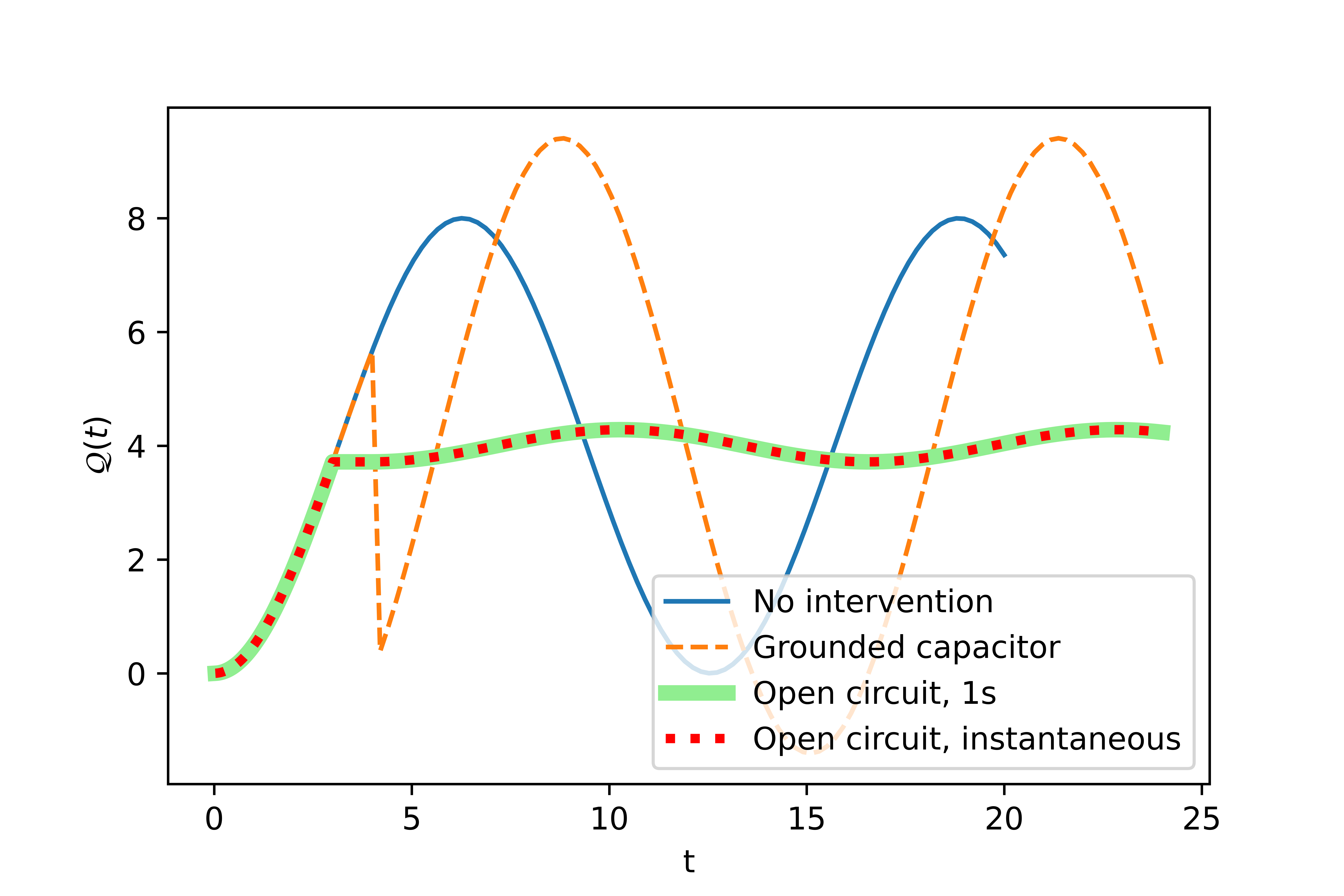
Figure 1: LC circuit outcomes under different interventions.

Now suppose that the capacitor breaks down if $\mathcal{Q}$ exceeds 6. Figure 1 shows that in the absence of intervention, $\mathcal{Q}$ exceeds 6 just after $t=4$. To prevent this, the operators ground the capacitor at time 4 (i.e., make the intervention $Q^{4}\leftarrow 0$). However, this does not help. As shown in Figure 1 (orange curve), this initially reduces $\mathcal{Q}$, but eventually it exceeds 6. Next, the operators try opening the circuit at time 3 and closing it again at time 4; that is, performing the intervention $K(3,4)\leftarrow 0$. (Recall that $K(3,4):=\{K^{t}\mid t\in(3,4)\}$.) This results in the circuit entering an operating regime where $\mathcal{Q}$ is nearly constant (the green curve in Figure 1), and never exceeds 6. We can show that, in agreement with intuition, the first intervention is not a cause of the capacitor not breaking down, and neither is the second (because it is not the minimal intervention required to bring about the outcome). But a sub-intervention $K^{4}\leftarrow 0$ of the second intervention is a cause (corresponding to the red curve in Figure 1). See Section 6 for details.

5 Related modeling techniques

We designed GSEMs as an extension of SEMs that can model systems with a continuous-time component. Many other causal or mechanistic modeling schemes have been proposed for such systems in the literature. In this section, we review three of these schemes: causal constraints models Blom et al. (2019), hybrid automata Alur et al. (1992), and counterfactual traces in rule-based models Laurent et al. (2018), and discuss their relationship to GSEMs. We remark that Ibeling and Icard [2019] consider SEMs with infinitely many variables and a second class of models that they call monotone simulation models. They show that monotone simulation models are equivalent to computable SEMs (ones where, roughly speaking, the structural equations are computable functions). Our examples showing that GSEMs are more general than SEMs apply immediately to the models considered by Icard and Ibeling.

5.1 Causal constraints models

At a coarse-grained level of modeling, such as when describing equilibrium solutions of dynamical systems, constraints between variables are natural objects of study. In order to describe equilibrium solutions and functional laws (roughly, dependencies that cannot be violated via intervention), Blom et al. (2019) introduced the notion of a causal constraints model (CCM). These models are composed of a set of constraints, each of which are active only under selected intervention targets; their outcomes under a given intervention are the solutions of the constraints active under the intervention’s target.

A CCM $M$ can be viewed as a pair $({\cal S},{\cal C})$, where ${\cal S}=({\cal U},{\cal V},{\cal R},{\cal I})$ is a signature and ${\cal C}$ is a set of causal constraints. Each constraint $C\in{\cal C}$ is a pair $(f_{C},a_{C})$, where $f_{C}:{\cal R}({\cal U})\times{\cal R}({\cal V})\to\{0,1\}$ and $a_{C}\subseteq{\cal P}({\cal V})$. Given a context ${\bf u}$ and an intervention $\mathaccent 382{X}\leftarrow\mathaccent 382{x}\in{\cal I}$, the outcomes $M({\bf u},\mathaccent 382{X}\leftarrow\mathaccent 382{x})$ are all assignments ${\bf v}$ to the variables of ${\cal V}$ such that, for all $C\in{\cal C}$ with $\mathaccent 382{X}\in a_{C}$, $C$ is satisfied (e.g., we have $f_{C}({\bf u},{\bf v})=1$) and ${\bf v}[\mathaccent 382{X}]=\mathaccent 382{x}$. Causal constraints models are equivalent to GSEMs.

Theorem 5.1

: For all GSEMs, there is an equivalent CCM, and vice versa.

Of course, if we restrict to CCMs that satisfy the axioms in $AX^{+}$ (resp. $AX^{+}_{rec}$), we can prove an analogue of Theorem 5.1 for GSEMs satisfying $AX^{+}$ (resp. $AX^{+}_{rec}$).

CCMs were designed for characterizing equilibrium solutions of dynamical systems. They seem less well suited for our intended applications, since they do not simplify the process of reasoning from the model specification (i.e., constraints) to solutions. Thus, even though they are equivalent in expressive power, we believe that CCMs and GSEMs will find complementary applications.

6 Actual causes

One important application of causal modeling is to deducing the actual cause(s) of $X=x$, that is (roughly speaking) the specific reasons that $X$ takes value $x$ in a given context ${\bf u}$ and outcome ${\bf v}$.

Many definitions of actual cause in SEMs have been proposed (e.g., Beckers and Vennekens (2018); Glymour and Wimberly (2007); Hitchcock (2001, 2007); Weslake (2015); Woodward (2003)). For definiteness, we use that of Halpern and Pearl [2005], as later modified by Halpern [2016], except that we further modify it to deal with allowed interventions (which were not considered in earlier definitions).

Definition 6.1

: [Actual cause] Given a causal model $M$, ${\bf u}\in{\cal R}({\cal U})$, and ${\bf v}\in{\cal R}({\cal V})$, $\mathaccent 382{X}=\mathaccent 382{x}$ is an actual cause of the event $\varphi$ in $(M,{\bf u},{\bf v})$ if the following three conditions hold:

AC1.

${\bf v}\models\mathaccent 382{X}=\mathaccent 382{x}$ and ${\bf v}\models\varphi$.

AC2.

There is some $\mathaccent 382{W}\subseteq{\cal V}$ and a setting $\mathaccent 382{x}^{\prime}$ of $\mathaccent 382{X}$ such that $\mathaccent 382{W}\leftarrow{\bf v}[\mathaccent 382{W}];\mathaccent 382{X}\leftarrow\mathaccent 382{x}^{\prime}\in{\cal I}$ and $(M,{\bf u})\models\langle\mathaccent 382{W}\leftarrow{\bf v}[\mathaccent 382{W}];\mathaccent 382{X}\leftarrow\mathaccent 382{x}^{\prime}\rangle\neg\varphi.$

AC3.

No proper subset of $\mathaccent 382{X}$ satisfies conditions AC1 and AC2.

Intuitively, this definition captures the fact that when reasoning about counterfactuals in a concrete scenario, we often want to fix some details $\mathaccent 382{W}$ to the values ${\bf v}[\mathaccent 382{W}]$ that they actually had in that scenario; see Halpern (2015) for more examples and motivation. That paper did not consider allowed interventions. To deal with allowed interventions, we insist that the intervention $\mathaccent 382{W}\leftarrow{\bf v}[\mathaccent 382{W}];\mathaccent 382{X}\leftarrow\mathaccent 382{x}^{\prime}$ appearing in AC2 above is allowed.

Using this formal definition of causality, we can verify the claims made in Section 4 that (1) the intervention $Q^{4}\leftarrow 0$ is not an (actual) cause of the capacitor not breaking down, but (2) the intervention $K^{4}\leftarrow 0$ is. Recall that the capacitor breaks down if $\mathcal{Q}$ exceeds 6, so the capacitor not breaking down corresponds to the statement $\varphi=\forall t>4,\;\mathcal{Q}(t)\leq 6.$ Claim 1 is obvious, because under the first intervention, $Q^{t}$ does exceed 6 (at, say, $t=10$). Thus ${\bf v}\models\neg\varphi$, where ${\bf v}$ is the outcome under $Q^{t}\leftarrow 0$, which violates AC1. For Claim 2, note that on intervention-free intervals, the solutions are periodic in time, with period $2\pi/\omega=2\pi\sqrt{L^{0}C^{0}}=4\pi\approx 12.6$. Since $\mathcal{Q}$ does not exceed 6 on the interval $(4,4+12.6)$, it will never exceed 6. Thus ${\bf v}\models\varphi$, where ${\bf v}$ is the outcome $K^{4}\leftarrow 0$, satisfying AC1. AC2 is satisfied, because if we instead set $K^{t}\leftarrow K(t)$ for $t\in(3,4)$ where $K(t)$ is the value $K^{t}$ had under the empty intervention, $Q^{t}$ does exceed 6 (at, say, $t=6$). (Here we are taking $\mathaccent 382{W}=\emptyset$.) Finally, AC3 is satisfied, because the intervention $K^{4}\leftarrow 0$ is on a single variable, and therefore minimal. As mentioned before, we deferred several more examples applying this definition of actual cause in dynamical systems (hybrid automata and rule-based models) for reasons of space.

7 Other dynamical systems models

7.1 Hybrid automata

Hybrid automata are a well-developed class of models for systems that have both continuous and discrete components Alur et al. (1992); for example, a thermostat controlling a heater to keep the temperature within a certain tolerance of a set point. The state variables for this system are both continuously varying in time (the temperature) and discretely changing in time (whether the heater is on). In this section, we show how to construct a GSEM model corresponding to an arbitrary hybrid automaton. We demonstrate our construction on a simple example from Henzinger (2000) and show how the resulting GSEM can be used to answer causal questions.

Mathematically, a hybrid automaton is a finite directed multigraph $G=(V,E)$, a set $\bm{\mathcal{X}}=\{\mathcal{X}_{1},...,\mathcal{X}_{n}\}$ of real-valued dynamical variables, and some predicates (discussed below). The states $v\in V$ are called control modes, and they represent the state of the discrete component of the system. The edges $e=(u,v,n)\in E$, where $u$ and $v$ are control modes and $n$ indexes the edge among all edges from $u$ to $v$, are called control switches, and they describe transitions between control modes. Recall that a multigraph is a graph which may have multiple edges between any given pair of nodes; different control switches between the same pair of control modes represent different modes of transition between them. For example, the heater may have multiple triggers that change its state from OFF to ON.

The semantics of a hybrid automaton is defined by predicates $\mathsf{init},\mathsf{flow},\mathsf{jump}$, and $\mathsf{inv}$. Possible starting configurations are given by $\mathsf{init}(v,\bm{\mathcal{X}})$. Possible continuous dynamics within a control mode are given by $\mathsf{flow}(v,\bm{\mathcal{X}},\bm{\dot{\mathcal{X}}})$, where $\bm{\dot{\mathcal{X}}}$ represents the vector of first derivatives. Possibly discontinuous changes are given by $\mathsf{jump}(e,\bm{\mathcal{X}},\bm{\mathcal{X}}^{\prime})$, where $\bm{\mathcal{X}}^{\prime}$ represents values at the conclusion of the change. Hard constraints are represented by $\mathsf{inv}(v,\bm{\mathcal{X}})$, which may be thought of as describing invariants of the different control modes. Hybrid automata are nondeterministic in general; all dynamics compatible with the automaton’s predicates are possible.

Let $A=(V,E,\bm{\mathcal{X}},\mathsf{init},\mathsf{flow},\mathsf{jump},\mathsf{inv})$ be a hybrid automaton. We now construct a GSEM $M$ corresponding to $A$. The endogenous variables are as follows. For each $\mathcal{X}_{i}\in\bm{\mathcal{X}}$, $M$ has real-valued variables $\{X_{i}^{t}\mid t\geq 0\}$ corresponding to the value of $\mathcal{X}_{i}$ at time $t$. $M$ also has $V$-valued variables $\{S_{t}\mid t\geq 0\}$ corresponding to the control mode of the system at time $t$. $M$ has a single exogenous variable with a single value, so there is only one (trivial) context.

The outcomes for intervention $\mathaccent 382{Y}\leftarrow\mathaccent 382{y}$ are, similar to ODEs, all assignments to the variables that (1), agree with $\mathaccent 382{Y}\leftarrow\mathaccent 382{y}$, and (2), are otherwise compatible with the predicates of the automaton. More precisely, ${\bf v}\in M({\bf u},\mathaccent 382{Y}\leftarrow\mathaccent 382{y})$ iff all the following conditions hold. For convenience, we define functions $\mathcal{X}_{i}(t)={\bf v}[X_{i}^{t}]$ for $i=1,\dots,n$, $\bm{\mathcal{X}}(t)=\left(\mathcal{X}_{1}(t),\dots,\mathcal{X}_{n}(t)\right)$, and $\mathcal{D}(t)={\bf v}[S_{t}]$.

HA1.

${\bf v}[\mathaccent 382{Y}]=\mathaccent 382{y}$.

HA2.

$\mathsf{init}({\bf v}[S_{t}],\bm{\mathcal{X}}(0))$ holds.

HA3.

For all $t$, $\mathsf{inv}({\bf v}[S_{0}],\bm{\mathcal{X}}(t))$ holds.

HA4.

For all $t\geq 0$, if $\bm{\mathcal{X}}(t)$ is not continuous, at least one of (a) or (c) below holds; and if $\mathcal{D}(t)$ is not continuous, at least one of (b) or (c) below holds.

1. $X_{i}^{t}\in\mathaccent 382{Y}$ for some $i=1,\dots,n$.

2. $S_{t}\in\mathaccent 382{Y}$.

3. There is an edge $e=(u,v,n)\in E$ such that $\mathsf{jump}(e,\lim_{s\to t^{-}}\bm{\mathcal{X}}(t),\bm{\mathcal{X}}(t))$ holds.

HA5.

Defining intervention-free intervals in the same way as in Section 4, the following holds. For all intervention-free intervals $(a,b)$ such that $\bm{\mathcal{X}}$ is continuous on $(a,b)$, we have that $\bm{\mathcal{X}}$ is right-continuous at $a$, differentiable on $(a,b)$, and its derivative $\bm{\dot{\mathcal{X}}}$ satisfies the flow condition $\mathsf{flow}({\bf v}[S_{t}],\bm{\mathcal{X}}(t),\bm{\dot{\mathcal{X}}}(t))$ for all $t\in(a,b)$.

Note that HA5 is analogous to the condition ODE3 in Section 4. The modeler is free to select a set of allowed interventions that fits the task at hand. In the example below, we choose ${\cal I}$ to be the set of finite compositions of point and interval interventions on the dynamical variables and control mode variables, but the outcomes of $M$ are well-defined for arbitrary interventions. This concludes the construction of $M$.

A simple thermostat and heater automaton given by Henzinger (2000) (with the flow conditions slightly simplified) is as follows. There is a single continuous variable $\mathcal{T}\in\bm{\mathcal{X}}$ and two control modes $V=\{\mathit{OFF},\mathit{ON}\}$. The system starts in OFF with $\mathcal{T}=20$, which is the desired set point. This defines $\mathsf{init}(v,\bm{\mathcal{X}})$. In OFF, the temperature drifts slowly downward; we have $\dot{\mathcal{T}}=-0.1$. An invariant of OFF is that $\mathcal{T}\geq 18$; if at any point $\mathcal{T}<18$, the system transitions to ON. Likewise, in ON, the temperature increases rapidly as $\dot{\mathcal{T}}=0.5$, and an invariant of ON is $\mathcal{T}\leq 22$. These conditions define $\mathsf{flow}(v,\bm{\mathcal{X}},\bm{\dot{\mathcal{X}}})$ and $\mathsf{inv}(v,\bm{\mathcal{X}})$. There are two control switches, $e_{\rm on}$ from OFF to ON, and $e_{\rm off}$ from ON to OFF. Finally, the heater can transition from OFF to ON when $\mathcal{T}<19$, and from ON to OFF when $\mathcal{T}>21$. Neither of these transitions affects the instantaneous value of $\mathcal{T}$; that is, $\mathcal{T}^{\prime}=\mathcal{T}$. These conditions define $\mathsf{jump}(e,\bm{\mathcal{X}},\bm{\mathcal{X}}^{\prime})$.

Let us analyze the GSEM $M$ corresponding to this automaton. In our case, since neither of the two possible discrete jumps change the value of $\mathcal{T}$, HA4 implies that $\mathcal{T}$ must be continuous everywhere it is not intervened on. Interventions on $\mathcal{T}$ are finite compositions of point and interval interventions. Furthermore, when $\mathcal{T}$ is not intervened on, it cannot change very quickly; by HA5, it must obey the flow condition (either $\dot{\mathcal{T}}=-0.1$ or $\dot{\mathcal{T}}=0.5$). Hence, given a time horizon $\tau$, $\mathcal{T}$ can cross the vertical lines $\mathcal{T}=19$ and $\mathcal{T}=21$ only finitely many times prior to $\tau$. The state of the heater is specified by the control mode $S^{t}$. By HA4, the heater switches ON only at times $t$ when the state of the heater (i.e., $S^{t}$) is intervened on, or when $\mathcal{T}<19$; likewise, the heater switches OFF only when $S^{t}$ is intervened on, or when $\mathcal{T}>21$. Again, interventions on the state of the heater are finite compositions of point and interval interventions. It follows that the state of the heater changes only a finite number of times before any given time horizon $\tau$. Hence, it is meaningful to talk about the heater discretely changing state—before any given time $\tau$, the heater turns on at $t_{1},t_{3}$ and so on, and turns off at $t_{2},t_{4}$ and so on.

Now that we have some intuition for the behavior of $M$, we examine how $M$ can be used to answer questions of actual cause. By HA2, the heater is initially OFF, and the temperature is initially $\mathcal{T}=20$. In the absence of intervention or discrete jumps, the heater will stay OFF and the temperature will drop at the rate of 0.1 per unit time.

Consider an outcome ${\bf v}$ where the heater does not turn on until, at $t=\frac{18-20}{-0.1}=20$, it is required to do so by HA3; specifically, by the invariant of OFF that $\mathcal{T}\geq 18$. If the heater had been on over any open subinterval $(a,b)$ of $[0,20)$, the temperature would have been higher than 18 by $t=20$ by at least $0.5(b-a)$. Hence, intuitively, the heater being off over any such subinterval should be considered a cause of $T^{20}=18$. However, if we fix any subinterval $(a,b)\subset[0,20)$ and ask the formal question of whether $S(a,b)=\mathit{OFF}$ is an actual cause of $T^{20}=18$ in $(M,{\bf u},{\bf v})$ (where $S(a,b)=\{S^{t}\mid t\in(a,b)\}$), we run into problems.

AC1 and AC2 both hold, but AC3 does not. AC1 holds, because ${\bf v}[S^{t}]=\mathit{OFF}$ for all $t\in[0,20)$, and ${\bf v}[T^{20}]=18$. AC2 holds, since if we choose $\mathaccent 382{W}=\emptyset$ and $\mathaccent 382{x}^{\prime}=\mathit{ON}$ (recall that $\mathaccent 382{X}=S(a,b)$ we find that the outcome ${\bf v}^{\prime}$ of $M$ under intervention $\mathaccent 382{X}\leftarrow\mathaccent 382{x}^{\prime}$ where the heater is on only during $(a,b)$ has ${\bf v}^{\prime}[T^{20}]=18+0.5(b-a)\neq 18$. However, AC3 does not hold, because the open subinterval $(a,b)$ contains other open subintervals for which AC1 and AC2 also hold, by the same arguments. This implies that there is no open interval on which the heater being off is an actual cause of $T^{20}=18$.

This creates a dilemma. Since turning the heater on results in $T^{20}>18$, a good definition of actual cause should provide for some cause. In this case, the resolution is that the equality $S^{t}=\mathit{OFF}$ for any point $t\in(0,20)$ is in fact an actual cause of $T^{20}=18$. This is because one of the solutions to $S^{t}\leftarrow 1$ has $H_{s}=\mathit{ON}$ for all $s$ in some nonempty interval starting at $t$, which as before implies $T^{20}>18$. So AC2 holds. AC1 clearly holds, and AC3 holds because $S^{t}\leftarrow 1$ is a point intervention, therefore minimal. We believe this resolution to the dilemma is always possible in hybrid automata (if point interventions are allowed), since we see no way of defining a hybrid automaton such that when the control mode is intervened on at a point in time, the control mode does not remain at the intervened value for some nonzero amount of time in some solution (although we have not attempted to prove this).

However, we see no reason for this resolution to work in general. Other models of dynamical systems may not respond in the same way to intervention. This resolution even fails for our example hybrid automaton, if it is modified so that point interventions are not allowed. In these cases, the definition of actual causality presented in Section 6 fails to provide for any cause of $T^{20}>18$ involving only the heater state. The issue is that AC3 requires a minimal cause; but minimal causes do not exist in general when causes can involve infinitely many variables. It is an open problem to find a new definition of actual cause that handles infinitely many variables well in general. One potential solution is to broaden the set of things that count as causes in infinitary settings. In the definition presented in Section 6, only conjunctions of equalities $X=x$ can be actual causes. One could consider expanding possible causes to include infinite disjunctions over these equalities, for example, the statement that there is some nonempty interval on which the heater is off:

$$\exists(a,b)\forall t\in(a,b)S^{t}=\mathit{OFF}.$$

However, we do not pursue this approach further in this paper.

Note that if we ask instead whether $S^{t}(a,b)=\mathit{OFF}$ is an actual cause of $T^{20}\leq 19$ instead, there are no problems. The answer is yes, iff $b-a=2$. This agrees with the natural intuition that the heater being off for a sufficiently short time is not enough to cause the temperature to be low. (There is nothing special about $19$; the solution for any value $x>18$ is similar.)

7.2 Rule-based models

A rule-based model is a dynamical system that transitions probabilistically between states, with the transition defined by rewrite rules. In this section, we construct a GSEM corresponding to the generic rule-based model given by Laurent et al. [2018].

Laurent et al. [2018] show how a rule-based model can describe a reaction between a set $S$ of substrates and a set $K$ of kinases. The state of the mixture at time $t$ is a binary relation $\mathsf{Bound}\subseteq S\times K$ that specifies which substrates are bound to which kinases, and a unary relation $\mathsf{Phos}\subseteq S\cup K$ that defines which substrates and kinases have a phosphate group attached. Chemical interactions between groups of molecules are intended to take place spontaneously, in an analogous fashion to radioactive decay. For example, if at time $t$ there is a substrate $s\in S$ and a kinase $k\in K$ such that $(s,k)\in\mathsf{Bound}$ and $s\notin\mathsf{Phos}$, then at time $t+\Delta t$, where $\Delta t$ is drawn from an exponential distribution with a time constant that depends on the rule being applied, $s$ will gain a phosphate group (unless in the meantime some other rule has changed the state of the mixture so that the precondition for $s$ and $k$ no longer holds). These updates are called events. Interventions correspond to blocking some interactions from taking place at specific times, for example, “between $t=1$ and $t=2$, even if $s$ and $k$ satisfy the above conditions, $s$ cannot gain a phosphate group.”

Laurent et al. explain how to simulate these dynamics using the following algorithm. For every possible target $\mathsf{Targ}$ of a rule $r$—in the example above, this would be every substrate-kinase pair $(s,k)$—sample from a Poisson process with parameter $\tau/\ln(2)$ to obtain a schedule of times when the rule applies to this target. Then, starting with the initial mixture and moving through time, whenever any rule applies according to the schedule, check if the rule’s condition—in our example $(s,k)\in\mathsf{Bound}\wedge s\notin\mathsf{Phos}$—is satisfied for the target, and that the rule is not currently blocked by an intervention. If these conditions hold, update the mixture using the rule’s mapping (e.g. $\mathsf{Phos}\mapsto\mathsf{Phos}\cup\{s\}$); otherwise, do nothing.

This algorithm can immediately be described in a GSEM model. In the example above, for each time $t\in[0,\infty)$ we would have binary endogenous variables $\mathsf{Bound}^{t}_{(s,k)}$ for each $s\in S,k\in K$, along with variables $\mathsf{Phos}_{x}^{t}$ for each $x\in S\cup K$. The exogenous variables correspond to the firing schedule; we have timestamped variables $T^{t}_{r,\mathsf{Targ}}$, one for each rule $r$, each target $\mathsf{Targ}$ compatible with that rule. (There are also exogenous variables describing the initial state of the mixture.) In order to match the intervention model of Laurent et al. (2018), we add additional binary variables $B^{t}_{r,\mathsf{Targ}}$. Intuitively, $B_{r,\mathsf{Targ}}^{t}=1$ means that the firing of rule $r$ applied to target $\mathsf{Targ}$ at time $t$ is blocked. Finally, for bookkeeping, we have binary endogenous variables of the form $X^{t}_{r,\mathsf{Targ}}$ that model whether rule $r$ actually fired on target $\mathsf{Targ}$ at time $t$. The unique outcome is specified in the obvious way: $X^{t}_{r,\mathsf{Targ}}$ is true exactly if, at time $t$, $\mathsf{Targ}$ satisfies the condition of $r$, $T^{t}_{r,\mathsf{Targ}}$ is true, and $B^{t}_{r,\mathsf{Targ}}$ is false. If $X^{t}_{r,\mathsf{Targ}}$ is true, then at time $t$ the state (i.e., the relations $\mathsf{Bound}$ and $\mathsf{Phos}$) gets updated using the rule’s mapping. Interventions such as the one above can simply be described by setting some of the $B^{t}_{r,\mathsf{Targ}}$ to false; we take the set of allowed interventions ${\cal I}$ to be all interventions of this form. The trace $T({\bf u},I)$ is simply the (countable) sequence of variables $X^{t}_{r,\mathsf{Targ}}$ (in ascending order of $t$) for which $X^{t}_{r,\mathsf{Targ}}=1$.

Laurent et al. [2018] defined notions of enablement and prevention. Enablement and prevention happen at the level of events, or updates to the mixture. Every event $e$ corresponds to a variable $X^{t}_{r,\mathsf{Targ}}$; it occurs if $X^{t}_{r,\mathsf{Targ}}=1$. We can think of the relations $\mathsf{Bound}$ and $\mathsf{Phos}$ as binary vectors; each entry in these vectors is called a site. For any given event to occur, certain sites must have certain values. Hence, intuitively, given two events $e,e^{\prime}$, $e$ enables $e^{\prime}$ if $e$ is the last event before $e^{\prime}$ that modifies some site to the value that is needed for $e$ to occur. Likewise, $e$ prevents $e^{\prime}$ (roughly) if $e$ is the last event before $e^{\prime}$ to set a site $s$, and it sets $s$ to a value such that $e$ cannot occur. Given a context ${\bf u}$ and an intervention $I\in{\cal I}$, they considered the difference between the trace $T({\bf u})$ and the trace $T({\bf u},I)$. They showed that for every element of the first sequence absent from the intervened sequence, a chain of enablements and preventions could be traced back from that element to an element that was directly blocked by $I$. That is, enablements and preventions were sufficient to explain why each element of $T({\bf u})$ no longer in $T({\bf u},I)$ was missing.

The notion of actual cause complements this analysis. For example, it follows from the sufficiency of enablements and preventions just discussed that if one rule firing is the actual cause of another rule firing, then a chain of enablements and preventions can be traced back from the trace entry for the second rule to the trace entry for the first. More precisely, if $B^{t}_{r,\mathsf{Targ}}=0$ is an actual cause of $X^{t^{\prime}}_{r^{\prime},\mathsf{Targ}^{\prime}}=1$ in context ${\bf u}$, then a chain of enablements and preventions can be traced back from $X^{t^{\prime}}_{r^{\prime},\mathsf{Targ}^{\prime}}$ to $X^{t}_{r,\mathsf{Targ}}$ in the pair of traces $T({\bf u})$, $T({\bf u},B^{t}_{r,\mathsf{Targ}}\leftarrow 1)$. Without going into the formalism of Laurent et al. (2018), a sketch of the proof of this claim is as follows. The actual cause statement implies that $X^{t^{\prime}}_{r^{\prime},\mathsf{Targ}^{\prime}}$ is in $T({\bf u})$ but not in $T({\bf u},B^{t}_{r,\mathsf{Targ}}\leftarrow 1)$, because the intervention $B^{t}_{r,\mathsf{Targ}}\leftarrow 1$ is the only one that can satisfy AC2 and AC3. (The other blocking variables take value zero in both outcomes $M({\bf u},\emptyset)$ and $M({\bf u},B^{t}_{r,\mathsf{Targ}}\leftarrow 1)$, so setting them to 0 is redundant and violates AC3.) The only element blocked by $B^{t}_{r,\mathsf{Targ}}\leftarrow 1$ is $X^{t}_{r,\mathsf{Targ}}$. Hence, a chain of enablements and preventions can be traced back from $X^{t^{\prime}}_{r^{\prime},\mathsf{Targ}^{\prime}}$ to $X^{t}_{r,\mathsf{Targ}^{\prime}}$.

Actual cause and the GSEM machinery can also be used to answer questions not addressed by the analysis of Laurent et al. [2018]. We can ask counterfactual questions like “What would the state at $t=7$ be if every kinase gained a phosphate group at time $t=5$?” (potentially corresponding to the addition of a test tube’s worth of phosphate solution) or “Is the fact that substrate $s$ was bound to kinase $k$ at $t=1$ the actual cause of kinase $k$ gaining a phosphate group at $t=2$?” For this reason, we believe that GSEMs are a useful addition to the rule-based causal modeling toolkit developed by Laurent et al.

8 Conclusion

While SEMs are a popular modeling framework in many application areas, they have a restrictive form that makes working with infinitely many variables difficult. This has led to attempts to construct application-specific causal models in the study of ordinary differential equations Blom et al. (2019) and molecular biology Laurent et al. (2018). GSEMs can capture all these applications, while retaining the input-output behavior of SEMs. Indeed, SEMs are equivalent to finite GSEMs that satisfy certain properties of SEMs (Halpern’s axioms $AX^{+}$ Halpern (2000)). Moreover, GSEMs are easy to use; converting a given dynamical model to a GSEM essentially reduces to setting up allowed interventions, as we demonstrate in examples of ordinary differential equation models, rule-based models, and hybrid systems. Any causal notion defined only in terms of the input-output behavior of SEMs can be straightforwardly carried over to GSEMs. We demonstrate this for the important criterion of actual cause, and show how to apply this criterion in examples. Thus, GSEMs are a unifying causal framework that permit modelers to apply the same notions (e.g., actual cause) across many different models of causality.

Acknowledgments:

We thank Sander Beckers for insightful comments on an earlier version of this paper. Work supported in part by NSF grants IIS-178108 and IIS-1703846, a grant from the Open Philanthropy Foundation, ARO grant W911NF-17-1-0592, and MURI grant W911NF-19-1-0217.

Appendix A An axiom system for causal reasoning

We now review the axiom systems considered by Halpern [2000] for reasoning about causality. Note that there are two slight differences between our presentation and that of Halpern. First, as we mentioned earlier, we have weakened the language of causal formulas so that primitive causal formulas are no longer parameterized by contexts. Thus, our language has formulas such as $[\mathaccent 382{Y}\leftarrow\mathaccent 382{y}](X=x)$ rather than $[\mathaccent 382{Y}\leftarrow\mathaccent 382{y}](X({\bf u})=x)$. Second, the list of axioms given below does not include two of Halpern’s axioms, which he called D10 and D11. D11 is a technical axiom that was needed only to reason about formulas with contexts (to reduce to formulas that mentioned ony one context); D10 says that there are unique outcomes, and is redundant in acyclic systems. A minor modification of Halpern’s proof shows that the axiom systems $AX^{+}$ and $AX^{+}_{rec}$ defined below (which are identical to the system Halpern called $AX^{+}$ and $AX^{+}_{rec}$, respectively, except that they omit the axioms D10 and D11) are sound and complete for SEMs and acyclic SEMs, respectively, with respect to the language that we are considering (just as Halpern’s versions of $AX^{+}$ and $AX^{+}_{rec}$ were sound and complete for his language); the proof is essentially identical to Halpern’s, so we omit it here. To axiomatize acyclic SEMs, following Halpern, we define $Y\leadsto Z$, read “$Y$ affects $Z$”, as an abbreviation for the formula

$$\begin{split}&\lor_{\mathaccent 382{X}\subseteq{\cal V},\mathaccent 382{x}\in{\cal R}(\mathaccent 382{X}),y\in{\cal R}(y),z\neq z^{\prime}\in{\cal R}(Z)}\\ &\quad([\mathaccent 382{X}\leftarrow\mathaccent 382{x}](Z=z)\land[\mathaccent 382{X}\leftarrow\mathaccent 382{x},Y\leftarrow y](Z=z^{\prime}));\end{split}$$

that is, $Y$ affects $Z$ if there is some setting of some endogenous variables $\mathaccent 382{X}$ for which changing the value of $Y$ changes the value of $Z$. This definition is used in axiom D6 below, which characterizes acyclicity.

Definition A.1

: $AX^{+}$ consists of axiom schema D0-D5 and D7-D9, and inference rule MP. $AX^{+}_{rec}$ results from adding D6 to $AX^{+}$.

• All instances of propositional tautologies.

• $[\mathaccent 382{Y}\leftarrow\mathaccent 382{y}](X=x\Rightarrow X\neq x^{\prime})$ if $x,x^{\prime}\in{\cal R}(X)$, $x\neq x^{\prime}$ (functionality)

• $[\mathaccent 382{Y}\leftarrow\mathaccent 382{y}](x\in{\cal R}(X))$ (definiteness)

• $\langle\mathaccent 382{X}\leftarrow\mathaccent 382{x}\rangle(W=w\land\mathaccent 382{Y}=\mathaccent 382{y})\Rightarrow\langle\mathaccent 382{X}\leftarrow\mathaccent 382{x};W\leftarrow w\rangle(\mathaccent 382{Y}=\mathaccent 382{y})$ (composition)

• $[\mathaccent 382{W}\leftarrow{\bf w};X\leftarrow x](X=x)$ (effectiveness)

• $(\langle\mathaccent 382{X}\leftarrow\mathaccent 382{x};Y\leftarrow y\rangle(W=w\land\mathaccent 382{Z}=\mathaccent 382{z})\land\langle\mathaccent 382{X}\leftarrow\mathaccent 382{x};W\leftarrow w\rangle(Y=y\land\mathaccent 382{Z}=\mathaccent 382{z}))$
  $\mbox{ }\ \ \ \Rightarrow\langle\mathaccent 382{X}\leftarrow\mathaccent 382{x}\rangle(W=w\land Y=y\land\mathaccent 382{Z}=\mathaccent 382{z})$, where $\mathaccent 382{Z}={\cal V}-(\mathaccent 382{X}\cup\{W,Y\})$ (reversibility)

• $(X_{0}\leadsto X_{1}\land\ldots\land X_{k-1}\leadsto X_{k})\Rightarrow\neg(X_{k}\leadsto X_{0})$ (recursiveness)

• $([\mathaccent 382{X}\leftarrow\mathaccent 382{x}]\varphi\land[\mathaccent 382{X}\leftarrow\mathaccent 382{x}](\varphi\Rightarrow\psi))\Rightarrow[\mathaccent 382{X}\leftarrow\mathaccent 382{x}]\psi$ (distribution)

• $[\mathaccent 382{X}\leftarrow\mathaccent 382{x}]\varphi$ if $\varphi$ is a propositional tautology (generalization)

• $\langle\mathaccent 382{Y}\leftarrow\mathaccent 382{y}\rangle true\wedge\big{(}\langle\mathaccent 382{Y}\leftarrow\mathaccent 382{y}\rangle(X=x)\Rightarrow\langle Y\leftarrow y\rangle(X\neq x^{\prime})\big{)}$, if $x\neq x^{\prime}$. (unique outcomes for ${\cal V}-\{X\}$)

• From $\varphi$ and $\varphi\Rightarrow\psi$, infer $\psi$ (modus ponens)

Appendix B Proofs

Theorem 2.1: If $M$ and $M^{\prime}$ are causal models over the same signature ${\cal S}$ that, given a context and intervention, return a finite set of outcomes, then $M$ and $M^{\prime}$ have the same outcomes (that is, for all ${\bf u}\in{\cal R}({\cal U})$ and $I\in{\cal I}$, $M({\bf u},I)=M^{\prime}({\bf u},I)$) if and only if they satisfy the same set of causal formulas (that is, for all ${\bf u}\in{\cal R}({\cal U})$ and $\psi\in{\cal L}({\cal S})$, $M,{\bf u}\models\psi\Leftrightarrow M^{\prime},{\bf u}\models\psi$).

Proof: Let $M$ and $M^{\prime}$ be causal models with the same set of solutions. It suffices to consider the primitive causal formulas $[\mathaccent 382{Y}\leftarrow\mathaccent 382{y}](X=x)$, since the truth of other formulas in ${\cal L}({\cal S})$ are derived from these. Recall that $M,{\bf u}\models{[\mathaccent 382{Y}\leftarrow\mathaccent 382{y}](X=x)}$ iff for all outcomes ${\bf v}\in M({\bf u},\mathaccent 382{Y}\leftarrow\mathaccent 382{y})$, ${\bf v}[X]=x$. But $M({\bf u},\mathaccent 382{Y}\leftarrow\mathaccent 382{y})=M^{\prime}({\bf u},\mathaccent 382{Y}\leftarrow\mathaccent 382{y})$, so $M,{\bf u}\models[\mathaccent 382{Y}\leftarrow\mathaccent 382{y}](X=x)$ if and only if $M^{\prime},{\bf u}\models[\mathaccent 382{Y}\leftarrow\mathaccent 382{y}](X=x)$. Conversely, suppose that $M$ and $M^{\prime}$ satisfy the same set of causal formulas. Suppose for contradiction that there exists some ${\bf u}$ and $I$ with $M({\bf u},I)\neq M^{\prime}({\bf u},I)$. Then without loss of generality, there is an outcome ${\bf v}$ in $M({\bf u},I)$ that is not in $M^{\prime}({\bf u},I)$. This outcome must differ from each of the finitely many outcomes $\{{\bf v}_{1},{\bf v}_{2},\dots,{\bf v}_{n}\}=M^{\prime}({\bf u},I)$ in at least one variable; that is, there must be variables $X_{1},X_{2},\dots,X_{n}\in{\cal V}$ with ${\bf v}[X_{i}]\neq{\bf v}_{i}[X_{i}]$ for $i\in 1,2,\dots,n$. Consider the causal formula $\varphi=\langle I\rangle(\bigwedge_{1\leq i\leq n}X_{i}={\bf v}[X_{i}])$. We have that $M,{\bf u}\models\varphi$, since ${\bf v}\in M({\bf u},I)$. However, it is not true that $M^{\prime},{\bf u}\models\varphi$, because no outcome ${\bf v}_{i}$ of $M^{\prime}$ satisfies $\bigwedge_{1\leq i\leq n}X_{i}={\bf v}[X_{i}]$. This contradicts the assumption s that $M$ and $M^{\prime}$ satisfy the same set of causal formulas; hence $M({\bf u},I)=M^{\prime}({\bf u},I)$ for all ${\bf u}\in{\cal R}(U)$, $I\in{\cal I}$.  

Theorem 3.1: For all SEMs $M$, there is a GSEM $M^{\prime}$ such that $M\equiv M^{\prime}$.

Proof: Given a SEM $M=(({\cal U},{\cal V},{\cal R},{\cal I}),{\cal F})$, define $M^{\prime}=(({\cal U},{\cal V},{\cal R},{\cal I}),{\cal F}^{\prime})$, where for all $\mathaccent 382{X}\leftarrow\mathaccent 382{x}\in{\cal I}$ and ${\bf u}\in{\cal U}$, ${\cal F}^{\prime}({\bf u},\mathaccent 382{X}\leftarrow\mathaccent 382{x})=M({\bf u},\mathaccent 382{X}\leftarrow\mathaccent 382{x})$. Since $M^{\prime}({\bf u},\mathaccent 382{X}\leftarrow\mathaccent 382{x})={\cal F}^{\prime}({\bf u},\mathaccent 382{X}\leftarrow\mathaccent 382{x})$, $M^{\prime}$ is equivalent to $M$ by definition.  

Theorem 3.2: For all SEMs $M$ and interventions $I,J\in{\cal I}$ such that $I;J\in{\cal I}$, we have that $M_{I}({\bf u},J)=M({\bf u},I;J)$.

Proof: We prove the equivalent statement $(M_{I})_{J}({\bf u})=M_{I;J}({\bf u})$. Since the outcomes of SEMs are determined by the structural equations, it suffices to show that the structural equations of $(M_{I})_{J}$ are the same as those of $M_{I;J}$. Let $X\in{\cal V}$ be arbitrary and consider the structural equation ${\cal F}_{X}$. Without loss of generality, let $I=\mathaccent 382{Y}\leftarrow\mathaccent 382{y}$ and $J=\mathaccent 382{Z}\leftarrow\mathaccent 382{z}$. There are three cases to consider: $X\notin\mathaccent 382{Y}\cup\mathaccent 382{Z}$, $X\in\mathaccent 382{Z}$, and $X\in\mathaccent 382{Y}\setminus\mathaccent 382{Z}$. The first case is trivial; ${\cal F}_{X}$ is unmodified in both models. In the second case, letting $\mathbb{s}\in{\cal R}({\cal V}\setminus\{X\})$ denote an arbitrary input to ${\cal F}_{X}$, in $(M_{I})_{J}$, we have that ${\cal F}_{X}(\mathbb{s})=\mathaccent 382{Z}[X]$. But by the definition of $I;J$, we also have ${\cal F}_{X}(\mathbb{s})=\mathaccent 382{Z}[X]$ in $M_{I;J}$. In the third case, in $(M_{I})_{J}$, ${\cal F}_{X}(\mathbb{s})=\mathaccent 382{Y}[X]$, since in $M_{I}$, ${\cal F}_{X}(\mathbb{s})=\mathaccent 382{Y}[X]$, and applying the intervention $J$ does not affect ${\cal F}_{X}$ since $X\notin\mathaccent 382{Z}$.  

Theorem 3.3: Suppose that $M$ and $M^{\prime}$ are causal models with $M\equiv M^{\prime}$. Then for all $I\in{\cal I}$, we have that $M_{I}\equiv M^{\prime}_{I}$.

Proof: Clearly $M_{I}$ and $M^{\prime}_{I}$ have the same signatures. It remains to show that for all contexts ${\bf u}$ and all intervention $J$ allowed in $M_{I}$, we have that $M_{I}({\bf u},J)=M^{\prime}_{I}({\bf u},J)$. Applying the definition and the fact that $M\equiv M^{\prime}$, we have that $M^{\prime}_{I}({\bf u},J)=M^{\prime}({\bf u},I;J)=M({\bf u},I;J)$. Therefore, it suffices to show $M({\bf u},I;J)=M_{I}({\bf u},J)$, which is exactly Theorem 3.2.  

The following theorem is needed to prove Theorem 3.4.

Theorem B.1

: If $M$ and $M^{\prime}$ are causal models (either SEMs or GSEMs) with a common signature ${\cal S}=({\cal U},{\cal V},{\cal R},{\cal I}_{univ})$, where ${\cal V}$ is finite and ${\cal R}(X)$ is finite for all $X\in{\cal V}$, that both satisfy the axioms in $AX^{+}$ and have the same outcomes under complete interventions—that is, for all ${\bf u}\in{\cal R}({\cal U})$ and $X\in{\cal V}$, if $\mathaccent 382{Y}={\cal V}\setminus X$, then for all $\mathaccent 382{y}\in{\cal R}(\mathaccent 382{Y})$, $M({\bf u},\mathaccent 382{Y}\leftarrow\mathaccent 382{y})=M^{\prime}({\bf u},\mathaccent 382{Y}\leftarrow\mathaccent 382{y})$—

then $M$ and $M^{\prime}$ agree on all causal formulas.

Proof: Fix an arbitrary context ${\bf u}$. $M$ satisfies axiom D9, so for every variable $X\in{\cal V}$, and for every assignment $\mathaccent 382{y}\in{\cal R}(\mathaccent 382{Y})$ to the variables $\mathaccent 382{Y}={\cal V}\setminus\{X\}$, there is a unique $x\in{\cal R}(X)$ such that $M,{\bf u}\models[\mathaccent 382{Y}\leftarrow\mathaccent 382{y}](X=x)$. Using this fact, we can define a SEM $M^{\prime\prime}$ with signature ${\cal S}$ as follows. Define ${\cal F}^{\prime\prime}_{X}({\bf u},\mathaccent 382{y})$ to be the unique $x$ such that $M,{\bf u}\models[{\cal V}\setminus\{X\}\leftarrow\mathaccent 382{y}](X=x)$. Let $C$ be the set of all formulas $\varphi=[{\cal V}\setminus\{X\}\leftarrow\mathaccent 382{y}](X=x)$ such that $M,{\bf u}\models\varphi$. By assumption, $C$ is also the set of all such formulas $\varphi$ for which $M^{\prime},{\bf u}\models\varphi$. Let $\chi$ be the conjunction of all the formulas in $C$. Since there are finitely many variables, and all ranges are finite, this set of formulas is finite, and so taking the conjunction makes sense. We know that $M$ and $M^{\prime}$ satisfy all axioms of $AX^{+}$, and both models satisfy $\chi$. This means that if $\chi\Rightarrow\psi$ is provable in $AX^{+}$, then $M$ and $M^{\prime}$ both satisfy $\psi$. We now show that, for all formulas $\psi$, either $\chi\Rightarrow\psi$ or $\chi\Rightarrow\neg\psi$ is provable in $AX^{+}$. This means that either both $M,{\bf u}\models\psi$ and $M^{\prime},{\bf u}\models\psi$ (if $\chi\Rightarrow\psi$ is provable in $AX^{+}$), or both $M,{\bf u}\nvDash\psi$ and $M,{\bf u}\nvDash\psi$ (if $\chi\Rightarrow\neg\psi$ is provable in $AX^{+}$). That is, $M$ and $M^{\prime}$ agree on all causal formulas. Note that $\chi$ is false in all SEMs over ${\cal S}$ other than models that agree with the $M^{\prime\prime}$ that we defined using $\chi$ in context ${\bf u}$. Thus, if $(M^{\prime\prime},{\bf u})\models\psi$, then $\chi\Rightarrow\psi$ is valid; and if $(M^{\prime\prime},{\bf u})\models\neg\psi$, then $\chi\Rightarrow\neg\psi$ is valid. Since $AX^{+}$ is a sound and complete axiomatization, it follows that either $\chi\Rightarrow\psi$ or $\chi\Rightarrow\neg\psi$ is provable, as desired.  

Theorem 3.4: For all finite GSEMs over a signature ${\cal S}$ such that ${\cal I}={\cal I}_{univ}$ and all the axioms of $AX^{+}$ are valid, there is an equivalent SEM, and vice versa.

Proof: Given a SEM $M$, define a GSEM $M^{\prime}$ with the same signature by taking ${\bf F}^{\prime}({\bf u},I)=M({\bf u},I)$, as in Theorem 3.1. This GSEM is clearly equivalent to $M$. Furthermore, all the axioms in $AX^{+}$ are valid in $M$. This follows from the facts that (1) equivalent causal models have the same outcomes (by definition), (2) finite causal models with the same outcomes satisfy the same causal formulas (Theorem 2.1), and (3) $M$ is a SEM, so all the axioms in $AX^{+}$ are valid in $M$. Conversely, given a finite GSEM $M^{\prime}$ in which all the axioms of $AX^{+}$ are valid, the GSEM must have unique solutions for ${\cal V}\setminus X$ (D9). That is, for each context ${\bf u}\in{\cal R}(U)$ and each variable $X\in{\cal V}$, if we define $\mathaccent 382{Y}={\cal V}\setminus X$, for every $\mathaccent 382{y}\in{\cal R}(Y)$, there is a unique $x\in{\cal R}(X)$ such that $M^{\prime},{\bf u}\models[\mathaccent 382{Y}\leftarrow\mathaccent 382{y}](X=x)$. Here we use the fact that ${\cal I}={\cal I}_{univ}$ to ensure that the relevant instances of D9 are in the language. We can use this property to define the structural equations of the SEM $M$. That is, define a SEM $M$ with the same signature by defining ${\cal F}_{X}({\bf u},\mathaccent 382{y})=x$, where $x$ is the value guaranteed above. We must show that $M$ has the same outcomes as $M^{\prime}$. But this is just Theorem B.1.  

Theorem 3.5: For all finite GSEMs over a signature ${\cal S}$ such that ${\cal I}={\cal I}_{univ}$ and all the axioms $AX^{+}_{rec}$ are valid, there is an equivalent acyclic SEM, and vice versa.

Proof: Given a finite GSEM $M^{\prime}$ satisfying $AX^{+}_{rec}$, Theorem 3.4 guarantees the existence of an equivalent SEM $M$. Since $M$ is equivalent to $M^{\prime}$, $M$ satisfies $AX^{+}_{rec}$. This implies that $M$ is acyclic. To prove this, suppose not. Then there is $k>1$ and endogenous variables $V_{1},\dots,V_{k}$ having cyclic dependencies; that is, $V_{i+1}$ is not independent of $V_{i}$ for $i=1,\dots,k-1$, and $V_{1}$ is not independent of $V_{k}$. But it is easy to see that if $Y$ is not independent of $X$, then $X$ affects $Y$, i.e., $X\leadsto Y$. Thus, $V_{k}\leadsto V_{1}\wedge V_{1}\leadsto V_{2}\wedge\dots\wedge V_{k-1}\leadsto V_{k}$. This is the negation of an instance of D6. Hence not all the axioms of $AX^{+}_{rec}$ are valid in $M$, a contradiction. For the converse, given an acyclic SEM $M$, Theorem 3.1 guarantees the existence of an equivalent GSEM $M^{\prime}$. This equivalent GSEM satisfies the same formulas as $M$, so it satisfies $AX^{+}_{rec}$.  

Theorem 4.1: The set of outcomes output by valid executions of SOLVE-ODE-GSEM are exactly the outcomes $M_{\mathit{ODE}}({\bf u},I)$.

Proof: We walk through the algorithm’s execution and show that whenever it defines a dynamical variable (and thus a model variable, via the translation in step 4), it can make all the choices compatible with ODE1, ODE2, and ODE3^′, and cannot make any other choices:

• In step 1, $\mathcal{X}_{i}(0)=X_{i}^{0}$ is the only choice consistent with the right-continuity requirement of ODE3^′.

• In step 2(a), $\mathcal{X}_{j}(t)=k$ is the only choice consistent with ODE1. It is compatible with ODE2 and ODE3, since ODE2 and ODE3 require nothing of intervened points.

• In step 2(b) and step 3, the possible settings for the intervention-free variables are exactly the settings allowed by ODE3^′. They are compatible with ODE1, since the intervention-free variables are not intervened on in $(a,b)$, and compatible with ODE2, since solutions to initial value problems are always continuous.

• In step 2(c)(i), $\mathcal{X}_{j}(t_{i})=\mathaccent 382{x}[X_{j}^{t_{i}}]$ is the only choice consistent with ODE1. It is compatible with ODE2 and ODE3 since, again, ODE2 and ODE3 require nothing of intervened points.

• In step 2(c)(ii), $\mathcal{X}_{j}(t_{i})=\lim_{t\to t_{i}^{-}}\mathcal{X}_{j}(t)$ is the only choice that maintains left-continuity (is consistent with ODE2). It is compatible with ODE1, since $\mathcal{X}_{j}$ is not intervened on at time $t_{i}$, and compatible with ODE3, since by construction, there is no intervention-constant open interval containing $t_{i}$. Finally, the limit always exists, because the values of $\mathcal{X}_{j}$ on $(t_{i-1},t_{i})$ were set in step 2(b), so $\mathcal{X}_{j}$ is continuous on the open interval $(t_{i-1},t_{i})$.

 

Theorem 5.1: For all GSEMs, there is an equivalent CCM, and vice versa.

Proof: Given a CCM $M^{\prime}=({\cal S},{\cal C},I)$, define a GSEM $M=({\cal S},{\bf F},{\cal I})$ by taking ${\bf F}({\bf u},I)=M^{\prime}({\bf u},I)$; it is immediate that $M$ and $M^{\prime}$ have the same outcomes. For the converse, given a GSEM $M=({\cal S},{\bf F},{\cal I})$, define a CCM $M^{\prime}=({\cal S},{\cal C},{\cal I})$ as follows. For every intervention $\mathaccent 382{X}\leftarrow\mathaccent 382{x}\in{\cal I}$, ${\cal C}$ contains a constraint $C_{\mathaccent 382{X}\leftarrow\mathaccent 382{x}}$ such that $a_{C_{\mathaccent 382{X}\leftarrow\mathaccent 382{x}}}=\{\mathaccent 382{X}\}$, and for every context ${\bf u}$, $f_{C_{\mathaccent 382{X}\leftarrow\mathaccent 382{x}}}({\bf u},{\bf v})=1$ iff either ${\bf v}[\mathaccent 382{X}]\neq\mathaccent 382{x}$ or ${\bf v}\in{\bf F}({\bf u},\mathaccent 382{X}\leftarrow\mathaccent 382{x})$. We claim that the outcomes $M^{\prime}({\bf u},\mathaccent 382{X}\leftarrow\mathaccent 382{x})$ are exactly the GSEM outcomes ${\bf F}({\bf u},\mathaccent 382{X}\leftarrow\mathaccent 382{x})$. Indeed, suppose ${\bf v}\in M^{\prime}({\bf u},\mathaccent 382{X}\leftarrow\mathaccent 382{x})$. Then ${\bf v}[\mathaccent 382{X}]=\mathaccent 382{x}$, and it follows from the constraint $C_{\mathaccent 382{X}\leftarrow\mathaccent 382{x}}$ that ${\bf v}\in{\bf F}({\bf u},\mathaccent 382{X}\leftarrow\mathaccent 382{x})$. For the opposite implication, suppose that ${\bf v}\in{\bf F}({\bf u},\mathaccent 382{X}\leftarrow\mathaccent 382{x})$. Then ${\bf v}[\mathaccent 382{X}]=\mathaccent 382{x}$ (since GSEMs satisfy effectiveness). Moreover, ${\bf v}$ satisfies all active constraints. It satisfies the constraint corresponding to $\mathaccent 382{X}\leftarrow\mathaccent 382{x}$, since ${\bf v}\in{\cal F}({\bf u},I)$. And it satisfies the constraints $C_{\mathaccent 382{X}\leftarrow\mathaccent 382{x}^{\prime}}$ for $\mathaccent 382{x}^{\prime}\neq\mathaccent 382{x}$, since ${\bf v}[\mathaccent 382{X}]=\mathaccent 382{x}\neq\mathaccent 382{x}^{\prime}$.  

Theorem B.2

: $M_{shell}$ satisfies all the axioms in $AX^{+}$.

Proof: D0, D1, D2, D7 and D8 are trivial. No joint interventions are allowed, so the only way to instantiate D3 is to have $\mathaccent 382{X}=W=S_{1}$ (or symmetrically, $\mathaccent 382{X}=W=S_{2}$). But if $\mathaccent 382{X}=W$, then $\mathaccent 382{X}\leftarrow\mathaccent 382{x};W\leftarrow w=W\leftarrow w$ and D3 follows trivially by eliminating the conjunction. D4 (effectiveness) holds by inspection. D5 holds for the same reason as D3. Finally, D9 cannot be instantiated because no complete interventions are allowed.

References

- Alur et al. [1992] R. Alur, C. Courcoubetis, T. A. Henzinger, and P.-H. Ho. Hybrid automata: An algorithmic approach to the specification and verification of hybrid systems. In Hybrid Systems, pages 209–229. Springer, 1992.
- Beckers and Halpern [2019] S. Beckers and J. Y. Halpern. Abstracting causal models. In Proc. Thirty-Third AAAI Conference on Artificial Intelligence (AAAI-19), 2019. The full version appears at arxiv.org/abs/1812.03789.
- Beckers and Vennekens [2018] S. Beckers and J. Vennekens. A principled approach to defining actual causation. Synthese, 195(2):835–862, 2018.
- Blom et al. [2019] T. Blom, S. Bongers, and J. M. Mooij. Beyond structural causal models: causal constraints models. In Proc. 35th Conference on Uncertainty in Artificial Intelligence (UAI 2019), 2019.
- Galles and Pearl [1998] D. Galles and J. Pearl. An axiomatic characterization of causal counterfactuals. Foundation of Science, 3(1):151–182, 1998.
- Glymour and Wimberly [2007] C. Glymour and F. Wimberly. Actual causes and thought experiments. In J. Campbell, M. O’Rourke, and H. Silverstein, editors, Causation and Explanation, pages 43–67. MIT Press, Cambridge, MA, 2007.
- Halpern and Pearl [2005] J. Y. Halpern and J. Pearl. Causes and explanations: a structural-model approach. Part I: Causes. British Journal for Philosophy of Science, 56(4):843–887, 2005.
- Halpern [2000] J. Y. Halpern. Axiomatizing causal reasoning. Journal of A.I. Research, 12:317–337, 2000.
- Halpern [2015] J. Y. Halpern. A modification of the Halpern-Pearl definition of causality. In Proc. 24th International Joint Conference on Artificial Intelligence (IJCAI 2015), pages 3022–3033, 2015.
- Halpern [2016] J. Y. Halpern. Actual Causality. MIT Press, Cambridge, MA, 2016.
- Henzinger [2000] T. A. Henzinger. The theory of hybrid automata. In Verification of Digital and Hybrid Systems, pages 265–292. Springer, 2000.
- Hitchcock [2001] C. Hitchcock. The intransitivity of causation revealed in equations and graphs. Journal of Philosophy, XCVIII(6):273–299, 2001.
- Hitchcock [2007] C. Hitchcock. Prevention, preemption, and the principle of sufficient reason. Philosophical Review, 116:495–532, 2007.
- Ibeling and Icard [2019] D. Ibeling and T. Icard. On open-universe causal reasoning. In Proc. 35th Conference on Uncertainty in Artificial Intelligence (UAI 2019), 2019.
- Laurent et al. [2018] J. Laurent, J. Yang, and W. Fontana. Counterfactual resimulation for causal analysis of rule-based models. In Proc. Twenty-Seventh International Joint Conference on Artificial Intelligence (IJCAI ’18), pages 1882–1890, 2018.
- Peters and Halpern [2021] S. Peters and J. Y. Halpern. Causal modeling with infinitely many variables. Available on arxiv., 2021.
- Rubenstein et al. [2017] P. K. Rubenstein, S. Weichwald, S. Bongers, J. M. Mooij, D. Janzing, M. Grosse-Wentrup, and B. Schölkopf. Causal consistency of structural equation models. In Proc. 33rd Conference on Uncertainty in Artificial Intelligence (UAI 2017), 2017.
- Weslake [2015] B. Weslake. A partial theory of actual causation. British Journal for the Philosophy of Science, 2015. To appear.
- Woodward [2003] J. Woodward. Making Things Happen: A Theory of Causal Explanation. Oxford University Press, Oxford, U.K., 2003.
- Young and Mohlenkamp [2017] T. Young and M. J. Mohlenkamp. Introduction to Numerical Methods and MATLAB Programming for Engineers. Ohio University, 2017. Available at https://openlibra.com/en/book/introduction-to-numerical-methods-and-matlab-programming-for-engineers.