Reinforcing RCTs with Multiple Priors
while Learning about External Validity

Abstract

This paper presents a framework for how to incorporate prior sources of information into the design of a sequential experiment. These sources can include previous experiments, expert opinions, or the experimenter’s own introspection. We formalize this problem using a Bayesian approach that maps each source to a Bayesian model. These models are aggregated according to their associated posterior probabilities. We evaluate a broad class of policy rules according to three criteria: whether the experimenter learns the parameters of the payoff distributions, the probability that the experimenter chooses the wrong treatment when deciding to stop the experiment, and the average rewards. We show that our framework exhibits several nice finite sample theoretical guarantees, including robustness to any source that is not externally valid.

Keywords: Reinforcement Learning, External Validity, RCTs, Bayesian Learning.

JEL: C11, C50, C90, O12.

[section1] [section1] 1

Table of Contents

1 Introduction

It has become increasingly common to replicate experiments from other settings. For example, conditional cash transfer programs now exist in over 60 countries throughout the world. In many of these countries, their implementation was accompanied by a rigorous impact evaluation (Garcia and Saavedra,, 2022). Other policy experiments that have been replicated in various settings include charitable giving (Karlan and List,, 2007), pay-for-performance schemes for teachers, charter schools (Chabrier et al.,, 2016), access to microcredit (Banerjee et al., 2015b, ), and BRAC’s ultra-poor graduation program (Banerjee et al., 2015a, ). Replication is also common in the private sector, as large tech firms frequently run thousands of experiments per years, often with only minor design variants (Thomke,, 2020).

Before replicating an experiment, the policymaker (or experimenter) may want to use previous information to determine how much experimentation is needed. Experiments can be costly to run, both in terms of implementation costs as well as opportunity cost. So if, on the one hand, the policymaker is certain that the documented benefits from the previous experiments will extrapolate to her setting then the learning gains from experimentation may not justify the costs, and she may want to scale the program from the start. On the other hand, if the policymaker’s is very uncertain then she may want to experiment first before expanding the program to scale.

Three issues lie at the heart of this decision. One is how much experimentation (versus exploitation) should our policymaker do? Two, how do we incorporate knowledge from previous experiments or experts into our decision process? And three, how does incorporating this knowledge affects the exploration versus exploitation tradeoff? In this paper, we propose a novel framework for how to incorporate previous sources of information in the design of an adaptive experiment.

Setup

We consider a policymaker who has to decide how to assign a set of treatments sequentially to an eligible population and when to stop the experiment. Subjects arrive in stages and at the beginning of each stage, the policymaker must first decide whether to stop the experiment. If she stops the experiment, she then assigns what she thinks is the best treatment to all subsequent subjects. But if the policymaker decides to continue the experiment, she assigns treatment just to the new arrivals and then moves onto a new stage. At each stage, the policymaker knows the history of previous treatment assignments and the corresponding realized outcomes, but does not know the probability distributions of potential outcomes, which she tries to learn about using the observed data. The policymaker does, however, have prior information about these distributions, which can arise from many sources, including her own introspection and knowledge, previous experiments, or expert opinions.

As the policymaker gathers more data from own experiment, she uses Bayes’ rule to update each of her prior sources and then takes a weighted average of each source’s posterior where the weights depend on how well the sources fit the observed data. On the basis of these beliefs, the policymaker then decides whether to stop the experiment and which treatment to assign.

In settings in which the policymaker must learn the truth, it is common not to use the optimal assignment rule, i.e. the one that maximizes her subjective payoff. This rule can have undesirable properties, such as failing to learn the correct treatment effects or being hard to compute and implement. As a result, the literature on multi-armed bandits have studied different heuristic rules such as $\epsilon$-greedy (Watkins,, 1989) and Thompson Sampling (Thompson,, 1933) and its refinements (e.g. Upper Confidence Bounds (Lai and Robbins,, 1985), or exploration sampling (Kasy and Sautmann,, 2021; Russo,, 2016)). We take a different approach and study a large class of policy rules that encompass, among others, the aforementioned examples. Importantly, we find that the only feature of the policy rule that matters for performance is the exploration structure – a sequence quantifying the amount of experimentation that occurs under a given policy rule at each stage of the experiment.

Performance Criteria

Given that optimality from the perspective of the policymaker may not be desirable, we evaluate our class of assignment rules on the basis of three regularly-used outcomes that are considered to be important from the point of view of an outside observer. Specifically, we explore whether the policymaker learns the true average treatment effects and at what rate. We also consider the likelihood that the policymaker does not choose the most beneficial treatment arm when deciding to stop the experiment. The third outcome measures the average payoff of the policymaker. Unlike the other two criteria, which are statistical in nature (i.e. they describe statistical properties of the experiment and its assignment rule), this outcome captures how much subjects benefit in net from the experiment both during and afterwards. When evaluated along these criteria, we can show, both theoretically and via Monte Carlo simulations, that our setup exhibits several nice finite sample properties and theoretical guarantees, including robustness to incorrect priors.

Main Findings

One of the contributions of our paper is that we provide a formal extension of the concept of external validity in the context of a Bayesian framework. In the classical, non-Bayesian setup a source is either externally validity or not. However in our setup, we can rank sources according to their degrees of external validity. Consequently, external validity under our definition is no longer a qualitative notion but rather a quantitative notion that depends on a bias variance tradeoff of the underlying source.

The ability to rank sources according to their degree of external validity appears in an important robustness property featured in our setup. Specifically, our model discards sources that do not extrapolate well to the current experiment, thereby exhibiting robustness to sources of information that are not externally valid. If relative to the other priors, one of the policymaker’s priors (about the average effects of the treatments) puts “low probability” on the true mean, then our approach will place close to zero weight on this source when aggregating across sources. Consequently, this prior will have little to no effect on the policymaker’s decisions or the learning rate. Similarly, sources whose priors put high probability on the truth receive higher weights that can approach one. This feature gives rise to an oracle type property wherein our concentration rates are close to those associated to the most externally valid source — the one with priors more concentrated around the truth — provided the other sources are sufficiently separated from this one.

Our setup also offers several theoretical guarantees. The policymaker will learn the average treatment effects, in the sense that her posterior mean of the potential outcome distribution concentrates around the true mean, and it does so at a rate of $1/(\sqrt{t}h^{2}_{t})$, where $t$ is the number of stages and $h_{t}$ is the amount of experimentation. That this concentration result holds was not obvious ex ante: in contrast to a standard randomized control trial setting, the policy functions in our setup are quite general and can depend on the entire history of play, thus creating time-dependence in the data. Nevertheless, by exploiting the concept of the exploration structure and Azuma-Hoeffding type concentration inequalities for Martingales, we not only obtain the rate of $1/(\sqrt{t}h^{2}_{t})$, but we can also characterize and quantify how this rate depends on the initial parameters of the setup.

Besides assigning treatments, our policymaker also has to consider when to stop the experiment and subsequently, what treatment to adopt. Both the duration of the experiment and adopting the correct treatment can have important welfare consequences. In our setup, the policymaker works with a class of stopping rules that stops the experiment when the average effect of a treatment is sufficiently above the others. This class of rules resembles the standard test of two means, but takes into account the fact that the data are not IID. Of course, whenever we stop an experiment, we worry about the possibility of making a mistake (i.e. not choosing the most beneficial treatment). We characterize the bounds on the probability of making a mistake for our setup. We show that these bounds decay exponentially fast with the length of the experiment, and that they are non-increasing in the degree of experimentation and in the size of the treatment effects. Moreover, we propose stopping rules that for any given tolerance level will yield a lower probability of making a mistake. Importantly, these stopping rules also exhibit an oracle property, whereby the upper bound on the probability of making a mistake is arbitrarily close to the upper bound of the unbiased source, provided the other sources are sufficiently separated from this one.

Finally, we also compute bounds for the rate at which the average observed outcomes converges to the maximum expected outcome. We show that the rate of convergence for these bounds are governed by an “exploitation versus exploration” trade-off. If we increase the degree of experimentation (less exploitation, more exploration) our data become more independent and the underlying uncertainty decreases. However, by exploring more, we are also increasing the bias associated with not choosing the optimal treatment. Unfortunately, these bounds are sufficiently complicated that we cannot characterize analytically the “optimal” degree of experimentation. Nevertheless, the results do suggest that pure experimentation (as in the case of an RCT) is unlikely to be optimal, and we verify this numerically in a series of simulations.

Charitable Giving

To further illustrate our procedure, we also present a proof-of-concept using data from a recent charitable fundraising experiment by Karlan and List, (2020). These types of experiments provide a nice test case because charitable giving is an outcome that responds relatively quickly to treatment. It is also an experiment that has been replicated in various settings (e.g. Karlan and List, (2007)), thus allowing for multiple priors. Using these data for our potential outcome distributions, we show that by incorporating multiple priors, our policymaker can stop the experiment in a third of the time, without a significant increase to the probability of making a mistake, thereby resulting in large performance gains relative to a standard RCT.

Contributions to the Literature

Our paper relates to three strands of the literature. First, we speak to an extensive multi-disciplinary literature on adaptive experimental design. Much of the focus of this literature has been on the multi-arm bandit problem, which considers how best to assign experimental units sequentially across treatment arms. Depending on the objective function, numerous studies have proposed a variety of alternative algorithms that, on average, outperform the static assignment mechanisms of traditional RCTs. In this paper, we focus less about constructing an alternative policy function than about on how to introduce information from different sources for a given class of policy functions. By doing so, the fundamental ‘earn vs learn’ tradeoff that characterizes the multi-arm bandit problem is not only a function of sampling variability in target data, but also uncertainty over the data generating process of the source data. To our knowledge, this is the first paper to propose a systematic, data-driven method to include multiple sources of information into the design of adaptive experiments.

Much of the literature on multi-armed bandits has focused on deriving bounds on expected regret for specific solution heuristics. Instead, we focus on alternative performance criteria, such as average outcomes, the probability of making a mistake, and concentration rates for posterior means, which to the best of our knowledge have not been formalized in a multi-prior multi-arm Bayesian bandit framework. Moreover, the results we derive are for a general class of solution heuristics, not a specific one. For these reasons, even though we do not view the technical results as the primary contribution of the paper, we do believe that they might be of independent interest even in standard multi-arm bandit problems. Furthermore, we view our paper as complementary to this existing literature, as techniques tailored for particular solution heuristics can be combined with our multi-prior Bayesian setting to obtain sharper theoretical guarantees.

By introducing issues of externality validity into the multi-arm bandit problem, our study also connects to the literature on measuring the generalizability of experiments. In general, scholars have taken three approaches for assessing external validity. One common approach is to measure how well treatment effect heterogeneity extrapolates to ‘left out’ study sites. Under the assumption that study site characteristics are independent of potential outcomes, a number of studies applying alternative estimators have interpreted the out-of-sample prediction errors as a measure or test of external validity. A related approach uses local average treatment effects across different complier populations to test for evidence of external validity (e.g. Angrist and Fernández-Val, (2013); Kowalski, (2016); Bisbee et al., (2017)). The general idea being that if differences in observable characteristics across subgroups explain differences in treatment effect heterogeneity then we can make some claim for external validity. A third common approach adopted in the meta-analysis literature is the use of hierarchical models to aggregate treatment effects across different study sites. A byproduct of this framework is a “pooling factor” across study sites that has a natural interpretation of generalizability. The factor compares the sampling variation of a particular study site to the underlying variation in treatment heterogeneity: the higher the measure, the larger the sampling error and the less informative the study site is about the overall treatment effect (e.g. Vivalt, (2020), Gelman and Carlin, (2014), Gelman and Pardoe, (2006), Meager, (2020)).

Our paper contributes to these approaches in two ways. First, we provide a formal definition for a subjective (Gaussian) Bayesian model to be externally invalid. Importantly, our definition offers a way to quantify or rank sources with different degrees of external validity. Second, we show that our particular belief aggregation method has the nice property that, as $t$ diverges, the weights are only positive for the least externally invalid models, allowing us to interpret these weights as measures of external validity.

While it is natural to interpret our measure of external validity in the context of other experiments, our setup is agnostic as to the source of the information and its level of uncertainty. Whether the policymaker’s priors come from previous experiments, observational studies, or expert opinions is immaterial for our setup. In this respect, our study also relates to a nascent, but growing literature measuring the extent to which experts can forecast experimental results (e.g. DellaVigna and Pope, (2018); DellaVigna et al., (2020)). Our paper provides a method for incorporating these forecasts in the design of policy evaluations in a manner that is robust to misspecified priors or behavioral biases (Vivalt and Coville,, 2021).

Organization of the Paper

The structure of the paper proceeds as follows. In Section 2, we set up the problem. We present two versions of the setup, one for the general model and the other for a Gaussian model. In Section 3, we provide analytical results for the Gaussian model. We then illustrate the main analytical results by simulation in Section 4. In Section 5, we illustrate our procedure using data from a charitable giving experiment. Section 6 concludes.

2 Setup

In this section, we describe the problem our policymaker (PM) aims to solve. Our PM’s problem consists of three parts: the experiment, the policy functions, and the learning framework.

2.1 The Experiment

The PM has to decide how to assign a treatment to a given unit (e.g. individuals or firms) and when to stop the experiment. We define an experiment by a number of instances $T\in\mathbb{N}$; a discrete set of observed characteristics of the unit, $\mathbb{X}$; a set of treatments $\mathbb{D}:=\{0,...,M\}$; and the set of potential outcomes. For now, we do not include a payoff function.

For each $(d,x)\in\mathbb{D}\times\mathbb{X}$, let $Y_{t}(d,x)\in\mathbb{R}$ denote the potential outcome associated with treatment $d$ and characteristic $x$ in instance $t$; also, let $Y_{t}(d):=(Y_{t}(d,x))_{x\in\mathbb{X}}$. Let $D_{t}(x)\in\mathbb{D}$ be the treatment assigned to the unit with characteristic $x$ in instance $t$. We denote the observed outcome of the unit with characteristic $x$ in instance $t$ as $Y_{t}(D_{t}(x),x)$.

The experiment has the following timing. At each instance, $t\in\{1,...,T\}$, the PM is confronted with $|\mathbb{X}|<\infty$ units, one for each value of the observed characteristic. At the beginning of the period, the PM decides whether to stop the experiment.

• If the PM decides to stop the experiment,

  • she chooses a treatment assignment at instance $t$ that will be applied to all subsequent units.

• If the PM does not stop the experiment,

  • she chooses a treatment assignment for each unit $x$ at time $t$.

  • Nature draws potential outcomes, $Y_{t}(d,x)$, for each unit.

  • The PM only observes the outcome corresponding to the assigned treatment, i.e. $Y_{t}(D_{t}(x),x)$.

We impose the following restriction on the data generating process for the vector of potential outcomes.

Assumption 1.

For each $t\in\{1,...,T\}$ and each $x\in\mathbb{X}$, $(Y_{t}(d,x))_{d\in\mathbb{D}}$ is drawn IID and $Y(d,x)\sim P(\cdot|d,x)\in\Delta(\mathbb{R})$.

Assumption 1 implies that units do not self-select across instances, i.e., the types of unit treated in instance $t$ are the same as the types treated in instance $t^{\prime}$. Implicit in this assumption and framework is also the absence of any selection into treatment or attrition, which is reasonable to assume for most experimental settings.

Finally, the assumption that the PM is confronted with $|\mathbb{X}|<\infty$ units, one for each value of the observed characteristic, is made out of convenience: it is straightforward to extended our theory to situations where the PM receives a random number of units, including zero, for each characteristic, provided this random number is exogenous. However, to extend the assumption of discrete covariates — $|\mathbb{X}|<\infty$ — to continuous ones is non-trivial. For learning in multi-arm bandits with continuous covariates, please see Dimakopoulou et al., (2017) and references therein, as well as Qin and Russo, (2022) who adapt the Thompson Sampling algorithm to handle a potentially non-stationary sequence of covariates influencing the arms’ performance.

The parameter of interest.

While this setup is sufficiently general to allow for any parameter of interest, we follow most of the literature and focus on the average treatment effect setup wherein the PM wants to learn

$$\theta(d,x):=E_{P(\cdot|d,x)}[Y(d,x)],\leavevmode\nobreak\ \forall(d,x)\in\mathbb{D}\times\mathbb{X}.$$

2.2 The Policy Rule

The policy rule associated with this experiment defines the behavior of the PM. We define it as a sequence of two policy functions that determine at each instance $t$, the probability of stopping the experiment and the probability of treatment for each $x\in\mathbb{X}$.

The first policy function, $(y^{t-1},d^{t-1})\mapsto\sigma_{t}(y^{t-1},d^{t-1})(x)\in[0,1]$, specifies the probability of stopping the experiment for unit $x\in\mathbb{X}$ given the observed history $y^{t-1},d^{t-1}$. The second policy function, $(y^{t-1},d^{t-1})\mapsto\delta_{t}(y^{t-1},d^{t-1})(\cdot|x)\in\Delta(\mathbb{D})$, specifies the probability distribution over treatments for each $x\in\mathbb{X}$; i.e., $\delta_{t}(Y^{t-1},D^{t-1})(d|x)$ is the probability that $x\in\mathbb{X}$ receives treatment $d$ given the past history. When there is no risk of confusion, we will omit the dependence on the history.

The policy rule defines two consecutive stages: a first stage of exploitation and exploration and a second stage of pure exploitation, in which the PM has stopped the experiment and has selected what she believes to be the best treatment. How the PM regulates the trade-off between exploitation and exploration in the first stage will be key for the results presented in Section 3. With this in mind, we now define a structure of exploration for the policy rule $(\delta_{t})_{t}$ as two positive-valued sequences $(h_{t},\omega_{t})_{t}$ such that for any $(d,x)\in\mathbb{D}\times\mathbb{X}$ and any $t\geq 0$, $\omega_{t}(d,x)\in[0,1]$, $h_{t}(\cdot|x)\in\Delta(\mathbb{D})$, and

$$\mathbf{P}\left(t^{-1}\sum_{s=1}^{t}\delta_{s}(d|x)\geq h_{t}(d|x)\right)\geq 1-\omega_{t}(d,x).$$ (2.1)

We call $(h_{t})_{t}$ the degree of exploration of the policy rule and $(1-\omega_{t})_{t}$ the likelihood of exploration of the policy rule. By providing a lower bound on the (average) propensity score, the structure of exploration quantifies the extent to which experimentation occurs under the policy rule $(\delta_{t})_{t}$. This structure is the only feature of the policy rule that matters for our performance criteria. We present these results formally in Section 3.

In Appendix K, we present several commonly-used policy rules — and their associated exploration structure — in the context of the Gaussian learning framework, which we describe next.

2.3 The Gaussian Learning Model

The PM does not know the probability distribution of potential outcomes $P$, but does have prior beliefs about it. This prior knowledge can come from many sources: the PM’s own prior knowledge, expert opinions, or past experiments. Importantly, we allow for multiple sources, in case the PM is unwilling or unable to discard one in favor of the others. If her prior sources of information extrapolate to the current experiment, then she should use them because they contain relevant information. But if some sources are not externally valid, then incorporating them in her assignment of treatment may lead to incorrect decisions, at least in finite samples. Thus, our PM not only faces the question of whether to incorporate the different sources, but how to aggregate them as well. We formalize this “external validity dilemma” by using a multiple prior Bayesian model.

Formally, for each $(d,x)\in\mathbb{D}\times\mathbb{X}$, the PM has a family of PDFs indexed by a finite dimensional parameter $\theta\in\Theta$, $\mathcal{P}_{d,x}:=\{p_{\theta}\colon\theta\in\Theta\}$, that describes what she believes are plausible descriptions of the true probability of the potential outcome $Y(d,x)$. The PM also has $L+1$ prior beliefs, $(\mu^{o}_{0}(d,x))_{o=0}^{L}$, regarding which elements of $\mathcal{P}_{d,x}$ are more likely; these prior beliefs summarize the prior knowledge obtained from the $L+1$ different sources.

For each $(d,x)\in\mathbb{D}\times\mathbb{X}$, the family $\mathcal{P}_{d,x}$ and the collection of prior beliefs give rise to $L+1$ subjective Bayesian models for $P(\cdot|d,x)$. Given the observed data of past treatments and outcomes, at instance $t\geq 1$, the PM will observe the realized outcome $Y_{t}(D_{t}(x),x)$ and the treatment assignment $D_{t}(x)$. Using Bayesian updating, she will then form posterior beliefs for each model, which we denote by $\mu^{o}_{t}(d,x)$. Observe that the belief is updated using observed data, $(Y_{t}(D_{t}(x),x),D_{t}(x))$ and using $p_{\theta}$ as the PDF of $Y_{t}(D_{t},x)$ given $D_{t}(x)=d$. That the belief for $(d,x)$ is only updated if $D_{t}(x)=d$ is analogous to the missing data problem featured in experiments under the frequentist approach.

We will further assume that the PM takes subjective models within the Gaussian family (see Section I in the Supplemental Material for the general setup). Formally, for each $(d,x)\in\mathbb{D}\times\mathbb{X}$, $\mathcal{P}_{d,x}$ is a family of Gaussian PDFs given by $\{\phi(\cdot;\theta,1)\colon\theta\in\mathbb{R}\}$ and the prior for every source is also assumed to be Gaussian with mean $\zeta^{o}_{0}(d,x)$ and variance $1/\nu^{o}_{0}(d,x)$. The quantity $\nu^{o}_{0}(d,x)$ can be interpreted as the number of units with characteristics $x$ that were assigned treatment $d$ in a past experiment. The higher the $\nu^{o}_{0}(d,x)$, the more certain source $o$ is about $\phi(\cdot;\zeta^{o}_{0}(d,x),1)$ being the correct model. Throughout, we will assume $(\zeta^{o}_{0},\nu^{o}_{0})_{o=0}^{L}$ are non-random.

Given the observed data of past treatments and observed outcomes, at instance $t$ the posterior belief, $\mu_{t}$, is also Gaussian with mean and inverse of the variance given by the following recursion: For any $t\geq 1$,

$$\zeta^{o}_{t}(d,x)= \frac{1\{D_{t}(x)=d\}}{\nu^{o}_{t-1}(d,x)+1\{D_{t}(x)=d\}}Y_{t}(d,x)+\frac{\nu^{o}_{t-1}(d,x)}{\nu^{o}_{t-1}(d,x)+1\{D_{t}(x)=d\}}\zeta^{o}_{t-1}(d,x)$$

$$= \frac{J_{t}(d,x)}{f_{t}(d,x)+\nu^{o}_{0}(d,x)/t}+\frac{\nu^{o}_{0}(d,x)/t}{f_{t}(d,x)+\nu^{o}_{0}(d,x)/t}\zeta^{o}_{0}(d,x)$$ (2.2)

$$\leavevmode\nobreak\ where$$

$$\nu^{o}_{t}(d,x)= N_{t}(d,x)+\nu^{o}_{0}(d,x),\leavevmode\nobreak\ f_{t}(d,x):=N_{t}(d,x)/t$$ (2.3)

$$\leavevmode\nobreak\ and\leavevmode\nobreak\ J_{t}(d,x):=t^{-1}\sum_{s=1}^{t}Y_{s}(d,x)1\{D_{s}(x)=d\}.$$ (2.4)

From these expressions, we can see how Gaussianity simplifies the dynamics of the problem in the two ways. First, we only need to analyze $(\zeta^{o}_{t}(d,x),\nu^{o}_{t}(d,x))_{t=0}^{T}$, a finite dimensional object, as opposed to $(\mu^{o}_{t}(d,x))_{t=0}^{T}$, an infinite dimensional object that is quite intractable. Second, it is easier to elicit priors in the Gaussian structure: We only need the average effect and the number of units assigned to each treatment arm. Furthermore, even with the Gaussianity assumption, our setup remains quite general in practice as we describe in the following remark.

Remark 2.1.

(1) Since the PM cares about learning the ATE, this model is sufficiently general to encompass the canonical RCT setup for estimation of average treatment effects, even when the potential outcomes are not necessarily Gaussian. To see this, note that even if the PM’s subjective model for potential outcomes is misspecified (i.e. she incorrectly assumes that $Y(d,x)$ is Gaussian) the PM can still accurately learn the true average effect because, for each $(d,x)$, there always exists a $\theta$ such that $\theta=E_{P(.|d,x)}[Y(d,x)]$. We show this is the case in Section 3.1.

(2) Our results and methodology extend to any subjective model whose posterior beliefs can be fully described by low finite-dimensional objects. For instance, in cases where $Y(d,x)\in\{0,1\}$, they extend to the Bernoulli-Beta model wherein the $t$ instance posterior is given by a Beta density with parameters given by $(\sum_{s=1}^{t}1\{D_{s}(x)=d\}Y_{s}(d,x)+\nu^{o}_{0}(d,x)\zeta^{o}_{0}(d,x),\sum_{s=1}^{t}1\{D_{s}(x)=d\}(1-Y_{s}(d,x))+\nu^{o}_{0}(d,x)(1-\zeta^{o}_{0}(d,x)))$. More generally, our methodology can be extended to the entire exponential family — which includes the models considered here and more (see Schlaifer and Raiffa, (1961) for examples), however, the interpretation of $\zeta_{t}(d,x)$ may change. $\triangle$

Model Aggregation & External Validity.

For each $(d,x)\in\mathbb{D}\times\mathbb{X}$ and faced with $L+1$ distinct subjective Bayesian models, $\{\langle\mathcal{P}_{d,x},\mu^{o}_{0}(d,x)\rangle\}_{o=0}^{L}$, our PM has to aggregate this information. There are different ways to do this; we choose one that at each instance $t$, averages the posterior beliefs of each model using as weights the posterior probability that model $o$ best fits the observed data within the class of models being considered, i.e.,

$$\mu^{\alpha}_{t}(d,x):=\sum_{o=0}^{L}\alpha^{o}_{t}(d,x)\mu^{o}_{t}(d,x)$$ (2.5)

where

$$\alpha^{o}_{t}(d,x):=\frac{\int\prod_{s=1}^{t}\phi(Y_{s}(d,x);\theta,1)^{1\{D_{s}(x)=d\}}\phi(\theta;\zeta^{o}_{0}(d,x),1/\nu^{o}_{0}(d,x))(\theta)d\theta}{\sum_{o=0}^{L}\int\prod_{s=1}^{t}\phi(Y_{s}(d,x);\theta,1)^{1\{D_{s}(x)=d\}}\phi(\theta;\zeta^{o}_{0}(d,x),1/\nu^{o}_{0}(d,x))(\theta)d\theta}.$$

We can interpret $\alpha^{o}_{t}(d,x)$ as the PM’s subjective probability that source $o$ for $(d,x)$ is more externally valid for her current experiment. To expound on this last point, we formalize a new definition of external validity within a (Gaussian) Bayesian framework.

Definition 1 (Degree of external validity).

For each $(d,x)\in\mathbb{D}\times\mathbb{X}$ the degree of external validity (DEV) of source $o$ is given by

$$\mathbb{EV}_{(d,x)}(o):=-\nu^{o}_{0}(d,x)(\theta(d,x)-\zeta^{o}_{0}(d,x))^{2}+\log\nu^{o}_{0}(d,x).$$

Given this definition, we can now partially order sources according to the next definition.

Definition 2 (Externally valid sources).

For $(d,x)$, a source $o$ is more externally valid than source a $o^{\prime}$ if has a higher degree of external validity, i.e.,

$$\mathbb{EV}_{(d,x)}(o)>\mathbb{EV}_{(d,x)}(o^{\prime}).$$

We denote this as $o\succ_{(d,x)}o^{\prime}$. A source $o$ is externally valid, if $\mathbb{EV}_{(d,x)}(o)=\infty$.

Given these definitions, it is useful to introduce some nomenclature. We call $|\zeta^{o}_{0}(d,x)-\theta(d,x)|$ the bias of source $o$ and $\nu^{o}_{0}(d,x)$ the degree of conviction of source $o$ — since a higher $\nu^{o}_{0}(d,x)$ implies a lower prior variance. As such, we can interpret $|\zeta^{o}_{0}(d,x)-\theta(d,x)|\sqrt{\nu^{o}_{0}(d,x)}$ as the degree of stubbornness of source $o$.

According to definition 1, the degree of external validity (DEV) of a given source is decreasing in its degree of stubbornness, holding the degree of conviction fixed. How the DEV depends on the degree of conviction is a bit more nuanced. To see this, observe that $\frac{d\mathbb{EV}_{(d,x)}(o)}{d\nu^{o}_{0}(d,x)}=-(\theta(d,x)-\zeta^{o}_{0}(d,x))^{2}+1/\nu^{o}_{0}(d,x)$. Thus, the effect of the degree of conviction on the DEV depends on the level of the bias. For unbiased sources, a higher degree of conviction can only increase the DEV. For biased sources, the effect is not uniform: For low initial values of conviction an increase in conviction will increase the DEV, but for high enough initial levels of conviction an increase of it will lower the DEV; i.e., the source is becoming more stubborn, re-affirming the bias. Finally, we note that the “cutoff" conviction level is inversely proportional to the level of the bias: A higher bias implies a larger range of initial conviction levels for which $\frac{d\mathbb{EV}_{(d,x)}(o)}{d\nu^{o}_{0}(d,x)}<0$; i.e., for more biased agents, conviction exacerbates their lack of external validity.

Figure 1 illustrates this discussion. The plot on the left presents the case where $o\succ_{(d,x)}o^{\prime}$ because even though both sources are unbiased, source $o$ has a higher level of conviction. In the middle plot, $o\succ_{(d,x)}o^{\prime}$, but now the the level of conviction is the same whereas the bias is lower for source $o$. Finally, the right plot illustrates the nuanced role of conviction: Source $o^{\prime\prime}$ (dashed black line) has a small bias but this gets amplified by a very high degree of conviction (i.e., it is highly stubborn), rendering it less externally valid than source $o^{\prime}$ (blue solid line) which is unbiased and with low degree of conviction; however source $o$ (solid red line) has the same small bias as source $o^{\prime\prime}$ but a degree of conviction that is lower than $o^{\prime\prime}$ but higher than $o^{\prime}$, rendering more externally valid that source $o^{\prime}$ and $o^{\prime\prime}$.

In sum, definitions 1 and 2 extend the concept of external validity to a Bayesian framework. In the classical — non-Bayesian — setup, bias defines whether a sources is externally validity (unbiased) or not (bias), as stated in Definition 2. However, this view of external validity is perhaps too narrow within a (Gaussian) Bayesian framework with a conviction level that may not be infinite. In this framework, external validity ceases to be a qualitative notion and becomes a quantitative notion which depends both on the bias and the level of conviction. This is precisely what our DEV measure captures.

Figure 1: Different Degrees of External Validity

The next proposition provides a link between this ranking of external validity and our weights $(\alpha^{o}_{t}(d,x))_{o=0}^{L}$. It shows that under some technical regularity assumptions, the weights are only positive for the least externally invalid models as $t$ diverges, provided $(d,x)$ is played sufficiently often.

Proposition 2.1.

For any $(d,x)\in\mathbb{D}\times\mathbb{X}$,

1. $\lim_{\mathbb{EV}_{(d,x)}(o)\rightarrow-\infty}\alpha^{o}_{t}(d,x)=0$.

2. If $\inf_{t}t^{-1}\sum_{s=1}^{t}\delta_{s}(d|x)>0$, then

   $$\alpha^{o}_{t}(d,x)=\frac{e^{0.5\mathbb{EV}_{(d,x)}(o)}}{\sum_{o^{\prime}=0}^{L}e^{0.5\mathbb{EV}_{(d,x)}(o^{\prime})}}+o_{\mathbf{P}}(1).$$

   In particular, if $o\succ_{(d,x)}o^{\prime}$, then $\alpha^{o^{\prime}}_{t}(d,x)<\alpha^{o}_{t}(d,x)+o_{\mathbf{P}}(1)$, and if $o$ is the externally valid source, then $\alpha^{o}_{t}(d,x)=1-o_{\mathbf{P}}(1)$.

Proof.

See Appendix B. ∎

Part (1) of the proposition shows that $\alpha^{o}_{t}$ offers certain robustness properties against externally-invalid models. If a source has a high degree of external invalidity — i.e., a very negative $\mathbb{EV}_{(d,x)}(o)$ —, then the associated weight of that source is approximately 0. Part (2) offers a sharper characterization of this robustness property, but asymptotically. It provides a link between the degree of external validity and the weight each source will have in the limit. In particular, sources that are less externally valid will receive less weight, and externally valid sources will get weight approaching one.

3 Analytical Results

Recall that the object of interest is the average effect of each treatment, and, at each instance $t$ and for each $(d,x)\in\mathbb{D}\times\mathbb{X}$, the PM estimates it using a subjective average treatment effect given by

$$\zeta^{\alpha}_{t}(d,x):=\int y\int_{\Theta}p_{\theta}(y)\mu^{\alpha}_{t}(d,x)(d\theta)dy=:\sum_{o=0}^{L}\alpha^{o}_{t}(d,x)\zeta^{o}_{t}(d,x).$$ (3.1)

The middle expression is the mean of the outcome computed with respect to the PM’s subjective PDF of $y$ constructed using the aggregate beliefs at instance $t$, $\int_{\Theta}p_{\theta}(\cdot)\mu^{\alpha}_{t}(d,x)(d\theta)$. The right-most expression shows the mean is the weighted average of the posterior mean for each source.

In this section, we establish some finite sample theoretical guarantees of this quantity, such as the rate at which it concentrates around the true average effect. Before we do so, a bit of housekeeping is required. Moving forward, we will omit $x$ from the notation and derive our results for $|\mathbb{X}|=1$. Given our assumptions, we can learn the fundamentals for each $x\in\mathbb{X}$ by treating them as separate and independent problems. Thus, we can extend all our results to the case of $|\mathbb{X}|>1$ by treating the relevant quantities (e.g. $\theta(d)$, $Y(d)$, etc.) as vectors of dimension $|\mathbb{X}|$. Furthermore, to derive the results below we will need some assumptions on the (true) distribution of the potential outcomes,

Assumption 2.

There exists a $\upsilon<\infty$ such that for any $\lambda>0$ and any $d\in\mathbb{D}$, $E[e^{\lambda(Y(d)-\theta(d))}]\leq e^{\upsilon\sigma(d)^{2}\lambda^{2}}$ where $\sigma(d)^{2}:=Var(Y(d))$.

This assumption imposes that $Y(d)$ is sub-gaussian. Sub-gaussianity plays two roles in our results. First, it ensures that some higher moments, like the variance, exist. Second, and more importantly, it is used to derive how fast the average outcome concentrates around certain population quantities (see Lemma D.1 in the Appendix D). A relaxation of this assumption will translate into slower concentration rates; see Remark D.1 in that appendix for more details.

Before presenting these results formally, it is useful to present our general approach for how we derived them. Given our key of object of interest is $\zeta^{\alpha}_{t}=\sum_{o=0}^{L}\alpha^{o}_{t}\zeta^{o}_{t}$, most of our results hinge on understanding how this object concentrates around the true expected value $\theta$.

For each treatment $d$, the randomness of $\zeta^{\alpha}_{t}(d)$ comes from two quantities: the frequency of play, $f_{t}(d)=t^{-1}\sum_{s=1}^{t}1\{D_{s}=d\}$ and the treatment-outcome average, defined as $J_{t}(d):=t^{-1}\sum_{s=1}^{t}1\{D_{s}=d\}Y_{s}(d).$ Hence, to derive the concentration rate of $\zeta^{\alpha}_{t}(d)$, we first need to understand how $f_{t}(d)$ and $J_{t}(d)$ concentrate. For $J_{t}(d)$, we can employ exponential inequalities for martingale differences (see Lemma D.1 in the Appendix D) to determine how fast the treatment-outcome average concentrates around $f_{t}(d)\theta(d)$. The case of $f_{t}(d)$ is a bit more nuanced because we care not only about how fast it concentrates around the average propensity score, $t^{-1}\sum_{s=1}^{t}\delta_{s}(d)$, but also about how far the average propensity score is from zero (i.e. the degree of exploration). Our structure of exploration allows the problem to be separated into two parts: we use exponential inequalities for martingale differences to determine the concentration rate and the structure of exploration to assess how far the average propensity score is from zero.

The next important step is to understand how the concentration rates of $f_{t}(d)$ and $J_{t}(d)$ translate into the concentration rate of $\zeta^{\alpha}_{t}(d)$ and how the parameters of the model and the exploration structure affect this rate. This is non trivial because, as expressions 2.2 and 3.1 show, there is a nonlinear mapping between these concentrations rate and the posterior mean. In fact, take any $\gamma,\eta>0$ where $\gamma$ and $\eta$ quantify the concentration rate of $J_{t}(d)$ around $f_{t}(d)\theta(d)$ and $f_{t}(d)$ around $t^{-1}\sum_{s=1}^{t}\delta_{s}(d)$ respectively. Given this and an exploration structure $(h_{t},\omega_{t})_{t}$, Lemma C.6 in the Appendix C.3 shows that

$$|\zeta^{\alpha}_{t}(d)-\theta(d)|\leq\Gamma(\gamma,h_{t}(d)-\eta,|\zeta_{0}(d)-\theta(d)|,\nu_{0}(d))$$ (3.2)

where $h_{t}(d)$ is the degree of exploration and $\Gamma:\mathbb{R}_{+}\times[0,1]\times\mathbb{R}^{L+1}\times\mathbb{N}^{L+1}\rightarrow\mathbb{R}$ is a function defined in Appendix C.3. This function $\Gamma$ is key for our results as it relates the concentration rate of the posterior mean around the true parameter to that of $J_{t}(d)$ and $f_{t}(d)$ (given by $\gamma$ and $\eta$ respectively), and also it tell us how the degree of exploration, the bias of each of the sources ($|\zeta_{0}(d)-\theta(d)|:=(|\zeta^{o}_{0}(d)-\theta(d)|)_{o=0}^{L}$) and the conviction of each of the sources ($|\nu^{o}_{0}(d)|:=(\nu^{o}_{0}(d))_{o=0}^{L}$) affect the posterior’s concentration rate. Moreover, Lemma C.5 in the Appendix C.3 shows that $\Gamma$ is increasing in the first argument and decreasing in the second one, thereby implying that a faster concentration rate of $J_{t}(d)$ and $f_{t}(d)$ translate into a faster concentration rate of the posterior mean.

3.1 Concentration bounds on the Posterior Mean

The next proposition establishes the rate at which the posterior mean concentrates around the true expected outcome.

Proposition 3.1.

For any $d\in\{0,...,M\}$, any $t\in\mathbb{N}$ and any $\varepsilon\geq 0$ such that $th_{t}(d)^{2}\geq\varepsilon$,

$$\mathbf{P}\left(|\zeta^{\alpha}_{t}(d)-\theta(d)|>\Gamma\left(\sqrt{\frac{2\upsilon\varepsilon}{h_{t}(d)^{2}t}}\sigma(d),0.5h_{t}(d),|\zeta_{0}(d)-\theta(d)|,\nu_{0}(d)\right)\right)\leq 4(e^{-\varepsilon}+\omega_{t}(d)).$$

Proof.

See Appendix E. ∎

The intuition behind the proof relies on the arguments discussed above that explain how the concentration rate of the posterior mean depends on two factors: the concentration rates of the random quantities $J_{t}(d)$ and $f_{t}(d)$ and how these get affected by the function $\Gamma$. More precisely, we show that by employing concentration inequalities for Martingale difference sequences (see Lemma D.1 in Appendix D), $J_{t}(d)$ and $f_{t}(d)$ are (up to constants) within $\gamma=\sqrt{\delta/t}$ and $\eta=h_{t}(d)\sqrt{\delta/t}$ of their respective population values with probability higher than $1-4e^{-\delta/h^{2}_{t}(d)}$ for any $\delta>0$. To obtain the final result, we simply plug these quantities into expression 3.2, while noting that $h_{t}(d)-\eta\geq 0.5h_{t}(d)$ for large enough $t$ and that $\varepsilon=\delta/h^{2}_{t}(d)$.

Through the term $\Gamma$ and the probability bound, the proposition illustrates the effect of the structure of exploration, $(h_{t},\omega_{t})_{t}$, on the concentration rates. In particular, $\Gamma$ is of order $O\left(\frac{(th^{2}_{t}(d))^{-1/2}}{h_{t}(d)+t^{-1}}\right)$ (see Lemma C.5(3) in the Appendix C.3). For policy functions with $h_{t}(d)\geq\epsilon>0$ (e.g. $\epsilon$-greedy) the concentration rate is of order $t^{-1/2}$, but for those with $h_{t}(d)=o(1)$ then the concentration rate is slower than this rate and consistency of the posterior mean to the truth is only ensured if $\sqrt{t}h^{2}_{t}(d)\rightarrow\infty$.

Our method for aggregating multiple priors offers an attractive feature regarding our concentration rates. Sufficiently stubborn models — i.e. $|\zeta^{o}_{0}(d)-\theta(d)|\sqrt{\nu^{o}_{0}(d)}$ is sufficiently large — will have close to zero effect on the concentration rate of $\zeta^{\alpha}_{t}(d)$, as they are essentially dropped from the weighted average. This implies an oracle property in the sense that the concentration rate becomes arbitrary close to the least stubborn model, provided there is enough separation between the stubbornness of this model and the others. We formalize this property in the next corollary.

Corollary 3.1.

Take any $(t,d,\varepsilon)$ as in Proposition 3.1. Furthermore, let model $o=0$ denote the least stubborn model and suppose that for any given $\delta>0$, there exists a $C$ such that $\min_{o\neq 0}|\zeta_{0}^{o}(d)-\theta(d)|\sqrt{\nu^{o}_{0}(d)}\geq C$. Then,

$$\mathbf{P}\left(|\zeta^{\alpha}_{t}(d)-\theta(d)|>\Omega\left(\sqrt{\frac{2\upsilon\varepsilon}{h_{t}(d)^{2}t}}\sigma(d),0.5h_{t}(d),|\zeta^{o}_{0}(d)-\theta(d)|,\nu^{o}_{0}(d)\right)+\delta\right)\leq 4(e^{-\varepsilon}+\omega_{t}(d))$$

Proof.

See Appendix E. ∎

The function $\Omega$, which is formally defined in Appendix C.2, acts as $\Gamma$ but for one model; i.e., for any $o\in\{0,...L\}$ and any $\gamma\geq 0$, assuming $J_{t}(d)$ and $f_{t}(d)$ are within $\gamma$ of their population analogues,

$$|\zeta^{o}_{t}(d)-\theta(d)|\leq\Omega(\gamma,h_{t}(d)-\gamma,|\zeta^{o}_{0}(d)-\theta(d)|,\nu^{o}_{0}(d)).$$

Thus, the expression inside the probability in the corollary is in fact the concentration rate of the least stubborn model.

We summarize the implications of the previous proposition in the following remark and illustrate them numerically in Section 4.

Remark 3.1 (Properties of the Concentration Rate).

The following properties are based on Lemma C.3 in Appendix C.2.

1. All else equal, the concentration rate decreases as the bias increases; it also decreases with the degree of stubbornness, i.e. $|\zeta^{o}_{0}(d)-\theta(d)|\sqrt{\nu^{o}_{0}(d)}$. The concentration rate is fastest when the bias is zero.

2. For confident models, the concentration rate increases with the degree of conviction, i.e. $\nu^{o}_{0}(d)$ increases. The intuition behind this result is as follows: If $\nu^{o}_{0}(d)$ increases but $|\zeta^{o}_{0}(d)-\theta(d)|\sqrt{\nu^{o}_{0}(d)}$ remains constant — equal to 0, in particular —, then necessarily, the model is becoming more convinced about a prior that is unbiased, thereby implying a faster convergence rate.

3. The effects of the degree of stubbornness and conviction on the concentration rate decrease as $t$ increases.

4. An increase in the degree of the exploration, $h_{t}(d)$, improves the concentration rate. This comes from the fact that $h_{t}(d)\mapsto\Omega\left(\sqrt{\frac{2\upsilon\varepsilon}{h^{2}_{t}(d)t}}\sigma(d),0.5h_{t}(d),|\zeta^{o}_{0}(d)-\theta(d)|,\nu^{o}_{0}(d)\right)$ is decreasing (see Lemma C.3 in the Appendix C.2). Intuitively, increasing $h_{t}(d)$ implies having more observations to estimate $\theta(d)$ — “more information” about treatment $d$ implies a faster concentration rate.

$\triangle$

3.2 Probability of making a mistake

In this section, we provide bounds on the probability of making a mistake. To do so, we need to define the policy rule for stopping the experiment, $\sigma$, since this rule governs the probability of making mistakes when stopping the experiment. A desirable property for this rule is that, for a given tolerance level $\beta\in(0,1)$ chosen by the PM, the probability of making a mistake when stopping the experiment is no larger than $\beta$. The following example provides one such rule:

Example 1 (Threshold Stopping Rule).

For any $x\in\mathbb{X}$ and any positive-valued non-increasing sequence $(\gamma_{t})_{t}$ and $B\in\mathbb{N}$, the stopping rule parameterized by $((\gamma_{t})_{t},B)$ is such that, for any $t\geq B$,

$$\sigma_{t}(Y^{t-1},D^{t-1})(x)=1,\leavevmode\nobreak\ iff\leavevmode\nobreak\ \max_{d}\{\min_{m\neq d}\zeta^{\alpha}_{t-1}(d,x)-\zeta^{\alpha}_{t-1}(m,x)-c_{t-1}(\gamma_{t-1},d,m,x)\}>0,$$

and if $t<B$, $\sigma_{t}(Y^{t-1},D^{t-1})(x)=0$, where, for any $d,m\in\{0,...,M\}$ and any $o\in\{0,...,L\}$,

$$c_{t}(\gamma_{t},d,m,x):c_{t}(\gamma_{t},d,x)+c_{t}(\gamma_{t},m,x):=\sum_{o=0}^{L}\gamma_{t}\frac{\alpha^{o}_{t}(d,x)}{f_{t}(d,x)+\nu^{o}_{0}(d,x)/t}+\sum_{o=0}^{L}\gamma_{t}\frac{\alpha^{o}_{t}(m,x)}{f_{t}(m,x)+\nu^{o}_{0}(m,x)/t}$$

where $f_{t}(d,x):=t^{-1}\sum_{s=1}^{t}1\{D_{s}(x)=d\}$. While the expression for the cutoff is a bit involved, the constant $\gamma_{t}$ is the key element – the other terms are convenient scaling factors. Loosely speaking, the proposition proposes to stop the experiment after $B$ instances and as soon as the distance between the highest average posterior and the rest — measured by $\max_{d}\min_{m\neq d}(\zeta^{\alpha}_{t}(d,x)-\zeta^{\alpha}_{t}(m,x))$ — is far enough from zero, where “far enough” is essentially measured by $Constant\times\gamma_{t}$. This rule is akin to a test of two means wherein the hypothesis is rejected when the difference in means is above a multiple of the standard error. This intuition suggests that $\gamma_{t}$ should be of order $1/\sqrt{t}$, however in this problem, as there are unknown quantities, the appropriate order is $\sqrt{\log t/t}$; see Section 3.2 for a more through discussion. $\triangle$

Suppose treatment $M$ has the largest expected effect, i.e., $\Delta:=\theta(M)-\max_{d\neq M}\theta(d)>0$. We define a mistake as recommending a treatment different than $M$ at the instance $t$ in which the experiment was stopped. Because recommendations are based on the PM’s posteriors, we can express a mistake as

$$\max_{d\neq M}\zeta^{\alpha}_{\tau}(d)-\zeta^{\alpha}_{\tau}(M)>0,$$

where $\tau$ indicates when the experiment is stopped, i.e., is the first instance after $B$ such that $\max_{d}\min_{m\neq d}\{\zeta^{\alpha}_{t}(d)-\zeta^{\alpha}_{t}(m)-c_{t}(\gamma_{t},d,m)\}>0$ where the cutoffs $c_{t}$ are defined in Example 1.

The following proposition provides an upper bound for the probability of making a mistake associated with this stopping rule, when all sources are unbiased or are biased but rank treatment $M$ as the highest one. For the general case where sources can be biased (in any direction), see Lemma F.1 in the Appendix F.

Proposition 3.2.

Suppose for each $d\in\{0,...,M-1\}$, $\zeta_{0}(d)\leq\theta(d)$ and $\zeta_{0}(M)\geq\theta(M)$. Consider the stopping rule defined in Example 1 with parameters $((\gamma_{t})_{t},B)$ then for any $t\geq 1$,

$$\mathbf{P}\left(\max_{d\neq M}\{\zeta^{\alpha}_{\tau}(d)-\zeta^{\alpha}_{\tau}(M)\}>0\right)\leq 2\sum_{d=0}^{M}\sum_{t=B}^{T}e^{-0.5t\frac{\gamma_{t}^{2}}{\upsilon\sigma(d)^{2}}}.$$ (3.3)

Proof.

See Appendix F. ∎

The intuition behind this proposition is as follows. Mistakes occur when, at some instance $t$ greater than $B$, the posterior mean of some treatment $d$ — different from $M$ — is “much larger" than the others. This implies that the posterior has to be “much larger” than its population mean, $\theta(d)$, where “much larger” depends on the pre-specified cutoff $\gamma_{t}$. Hence, given our assumption on the priors, the probability of a mistake is essentially given by the probability that, for some instance after $B$, the outcome-treatment average exceeds its population value by an amount given by $\gamma_{t}$. Lemma D.1 in Appendix D provides the bound of $e^{-0.5t\frac{\gamma_{t}^{2}}{\upsilon\sigma(d)^{2}}}$. Finally, since the stopping time is random and can ocurr at any instance after $B$, we sum over all possible such values of $t$.

In Proposition 3.2, we assumed unbiased sources or that the priors ranked treatment $M$ as the highest. In the next collorary, we can prove that when some sources are biased, there still exists an oracle property akin to the one demonstrated for the concentration rates. In particular, we show that upper bound is arbitrary close to the unbiased source, provided the other sources are sufficiently biased.

Corollary 3.2.

Let $o=0$ denoted the unbiased source. There exists a $C$ such that, if $\min_{o\neq 0}|\zeta^{o}_{0}(.)-\theta(.)|\geq C$ and $\zeta^{0}_{0}(.)=\theta(.)$, then

$$\mathbf{P}\left(\max_{d\neq M}\{\zeta^{\alpha}_{\tau}(d)-\zeta^{\alpha}_{\tau}(M)\}>0\right)\leq\sum_{d=0}^{M}\sum_{t=B}^{T}2e^{-0.5t\frac{(\gamma_{t})^{2}}{\upsilon\sigma(d)^{2}}}.$$

Proof.

See Appendix F. ∎

Proposition 3.2 also reveals how by properly choosing $((\gamma_{t})_{t},B)$, the probability of a mistake associated with the stopping rule is bounded by $\beta$, where $\beta\in(0,1)$ is any tolerance level. The next corollary presents such result.

Corollary 3.3.

Suppose all the conditions of Proposition 3.2 hold, and, for any $t$, $\gamma_{t}\geq\sqrt{\frac{\log t}{t}}\sqrt{A\log t}$ with $(A,B)$ such that $\log B\geq\max_{d}2\upsilon\sigma(d)^{2}$, and

$$\frac{3(M+1)}{A-1}(B^{-(A-1)}-T^{-(A-1)})\leq\beta.$$ (3.4)

Then

$$\mathbf{P}\left(\max_{d\neq M}\{\zeta^{\alpha}_{\tau}(d)-\zeta^{\alpha}_{\tau}(M)\}>0\right)\leq\beta.$$

Proof.

See Appendix F. ∎

We conclude by pointing out two technical features of this result. First, the sequence $(\gamma_{t})_{t}$ has to decay, at most, at $\log t/\sqrt{t}$ rate. Compared to the $1/\sqrt{t}$ rate that arises in the canonical difference of means test in statistics, we lose a factor of $\log t$. This factor acts as an upper bound for the unknown population quantities. If one knew or could estimate these quantities — the same way one estimates the standard deviations in the difference in means test — one could lose this extra $\log t$ factor. Second, the sequence $(\gamma_{t})_{t}$ can decay much slower than $\log t/\sqrt{t}$ — in fact, it may not decay at all. However, large values of $\gamma$ are undesirable because, the larger the $\gamma$, the less likely it is to stop the experiment at any instance thereby implying longer — and more costly — experiments. We therefore recommend to set $\gamma_{t}=O\left(\frac{\log t}{\sqrt{t}}\right)$.

3.3 Average Observed Outcomes

In this section, we characterize the behavior of the average outcome $t^{-1}\sum_{s=1}^{t}Y_{s}$. By Lemma D.1 in Appendix D, $t^{-1}\sum_{s=1}^{t}Y_{s}$ will concentrate around a weighted average of $\theta(\cdot)$, with the time average of the propensity score as weights, i.e.,

$$t^{-1}\sum_{s=1}^{t}\sum_{d=0}^{M}\theta(d)\delta_{s}(d).$$

Without further knowledge of $(\delta_{t})_{t}$, it is nearly impossible to characterize this average any further. However, for generalized $\epsilon$-greedy policy functions, indexed by a non-random sequence $\boldsymbol{\Xi}:=(\Xi_{t})_{t}$:

$$\delta_{t}(d)=\Xi_{t}(M+1)^{-1}+(1-\Xi_{t})1\{d=\arg\max_{a}\zeta^{\alpha}_{t-1}(a)\},\leavevmode\nobreak\ \forall t\in\{1,...,T\},$$ (3.5)

we can establish the following proposition for unbiased sources (the general result for biased sources can be found in Lemma G.2 in the Appendix G).

Proposition 3.3.

Suppose all sources are unbiased. For any $\gamma>0$ and any $t\in\{1,...,T\}$

$$\mathbf{P}\left(\max_{d}\theta(d)-t^{-1}\sum_{s=1}^{t}Y_{s}>-\mathcal{S}(t)-\mathcal{E}(t,\gamma,\bar{\Xi}_{t})-\mathcal{B}(\bar{\Xi}_{t})\right)\leq 5e^{-\gamma}.$$

where

$$\mathcal{S}(t,\gamma):= \sqrt{\frac{\gamma}{t}}\left(\sqrt{2\upsilon}\sigma(d)+\frac{||\theta||_{1}}{2}\right)\leavevmode\nobreak\ and\leavevmode\nobreak\ \mathcal{E}(t,\gamma,\bar{\Xi}_{t}):=2||\theta||_{1}\sqrt{1-\bar{\Xi}_{t}}\sqrt{e^{\gamma}\sum_{d=0}^{M}t^{-1}\sum_{s=1}^{t}\omega_{s-1}(d)}$$

$$with\leavevmode\nobreak\ \mathcal{B}(\bar{\Xi}_{t}):= ||\theta||_{1}\frac{\bar{\Xi}_{t}}{M+1},\leavevmode\nobreak\ with\leavevmode\nobreak\ \bar{\Xi}_{t}:=t^{-1}\sum_{s=1}^{t}\Xi_{s}.$$

Proof.

See Appendix G. ∎

Despite the length of the proposition, its parts are quite intuitive. The term $\mathcal{S}(t,\gamma)$ controls the stochastic error that arises from the difference between $t^{-1}\sum_{s=1}^{t}Y_{s}=\sum_{d=0}^{M}t^{-1}\sum_{s=1}^{t}Y_{s}(d)1\{D_{s}=d\}$ and its conditional expectation $\sum_{d=0}^{M}t^{-1}\sum_{s=1}^{t}\theta(d)\delta_{s}(d)$. This term is essentially of order $O(\sqrt{\gamma/t})$. The term $\mathcal{E}(t,\gamma,\bar{\Xi}_{t})$ arises from choosing the wrong treatment in the “exploitation" part because the policy function depends on $\zeta^{\alpha}$ and not $\theta$. It is decreasing on the quantity $\bar{\Xi}_{t}$, which regulates the trade-off between exploitation and exploration and can be viewed as the degree of exploration. A higher degree of exploration will result on more information about the treatment and in turn a smaller likelihood of choosing the wrong treatment. Finally, the term $\mathcal{B}(\bar{\Xi}_{t})$ is a non-random bias that stems from the “exploration” part of the policy function: With probability $\bar{\Xi}_{t}(M+1)$ the treatment is chosen at random, producing $\sum_{d=0}^{M}\theta(d)/(M+1)$.

If $\bar{\Xi}_{t}=t^{-1}\sum_{s=1}^{t}\sum_{d=0}^{M}\omega_{s-1}(d)=o(1)$, i.e., if the exploration part of the policy function vanishes, then $\gamma$ can be chosen to diverge with $t$, however slowly, and so, with probability approaching one, $t^{-1}\sum_{s=1}^{t}Y_{s}$ converges to $\max_{d}\theta(d)$.

The term $\mathcal{E}(t,\gamma,\bar{\Xi}_{t})+\mathcal{B}(\bar{\Xi}_{t})$ illustrates the so-called “exploration vs. exploitation” tradeoff and how it is regulated by $\bar{\Xi}_{t}$. This tradeoff suggests a choice for $\bar{\Xi}_{t}$ that balances $\mathcal{B}(\bar{\Xi}_{t})$ and $\mathcal{E}(t,\gamma,\bar{\Xi}_{t})$. Unfortunately, such a choice is infeasible as both terms depend on unknown quantities. Nevertheless, we can conclude that $\boldsymbol{\Xi}=1$ — the choice used in RCTs — will typically not be optimal. In fact, as $t$ increases, the “optimal” $\Xi_{t}$ will decrease to $0$, favoring “exploitation” to “exploration”. We explore the choice of $\boldsymbol{\Xi}$ further, when we simulate our model in the next section.

4 Model Simulations

In this section, we present Monte Carlo simulations of our model using the generalized $\epsilon$-Greedy policy rule presented in Equation 3.5. The purpose of these simulations is to highlight different aspects of our analytical results and to provide a sense of the tightness of our analytic bounds. We consider the case with only two treatment arms, $D\in\{0,1\}$, and assume that $Y(0)\sim N(1,1)$ and $Y(1)\sim N(1.3,1)$. We assess the performance of our model according to the three outcomes outlined in Section 3: concentrations bounds, probability of making a mistake, and average earnings. We simulate each experiment 1000 times, with each experiment lasting at most 1000 instances.

Multiple Priors, External Validity, Robustness

We begin by illustrating how our setup weights the different models over the course of the experiment. Recall that to aggregate across several distinct subjective Bayesian models, our setup will average the posterior beliefs of each model using as weights, $\alpha_{t}^{o}(d)$ – the posterior probability that model $o$ best fits the observed data within the class of models being considered. We demonstrated in Proposition 2.1 that if there exists an externally valid model among externally invalid models, then $\alpha_{t}^{o}(d)$ will approach one for the externally valid model. Conversely, $\alpha_{t}^{o}(d)$ will approach zero if models are far from the true $\theta(d)$.

To illustrate this property, we simulate our model under different sets of priors. For each simulation, we assume that our policymaker has two sets of priors about the potential outcomes distributions. One is her initial set of priors, which we will assume are correct (i.e. $\zeta^{o}_{o}=\theta$) but diffuse (i.e. $\nu$=1). For the other set of priors, we consider four alternative scenarios varying in their degree of stubbornness.

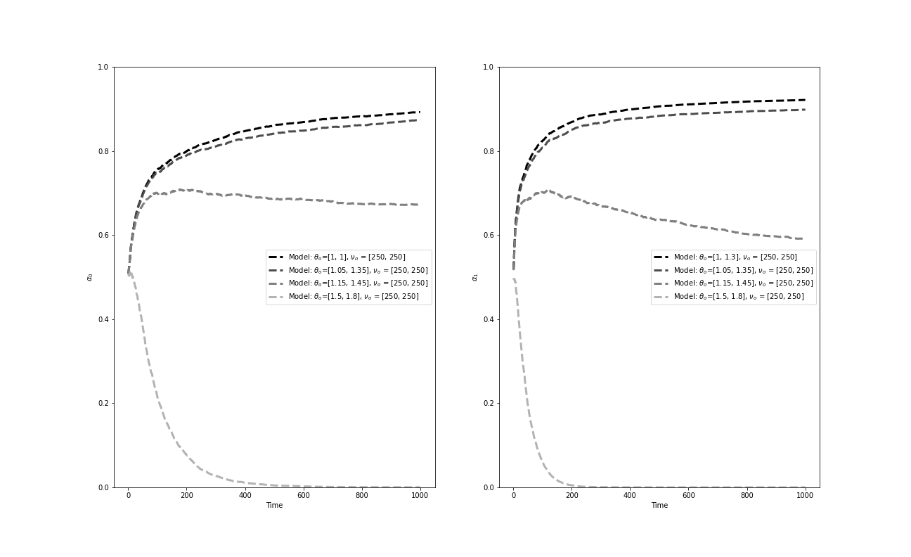
Figure 2: External Validity - $\alpha^{o}_{t}$

In Figure 2, we plot $\alpha_{t}^{o}(d)$ corresponding to the second set of priors over the course of the experiment. The graph on the left is for the $d=0$ arm and the one on the right is for the $d=1$ arm. Each line corresponds to a different set of priors, and the lighter the line, the more stubborn the prior. Starting with the top and darkest line, we see that $\alpha_{t}^{o}(d)$ increases over time putting more and more weight on an externally valid model. By the end of the experiment, $\alpha_{t}^{o}(d)$ is close to 95% for both arms. As we consider more stubborn models, we can see that the corresponding $\alpha_{t}^{o}(d)$ becomes smaller. So much so that for extremely stubborn models (i.e. the lowest line) $\alpha_{t}^{o}(d)$ becomes essentially zero by the $600^{th}$ instance. This is why we interpret the parameter $\alpha_{t}^{o}(d)$ as a measure of external validity: the more externally valid the model, the higher the corresponding $\alpha_{t}^{o}(d)$.

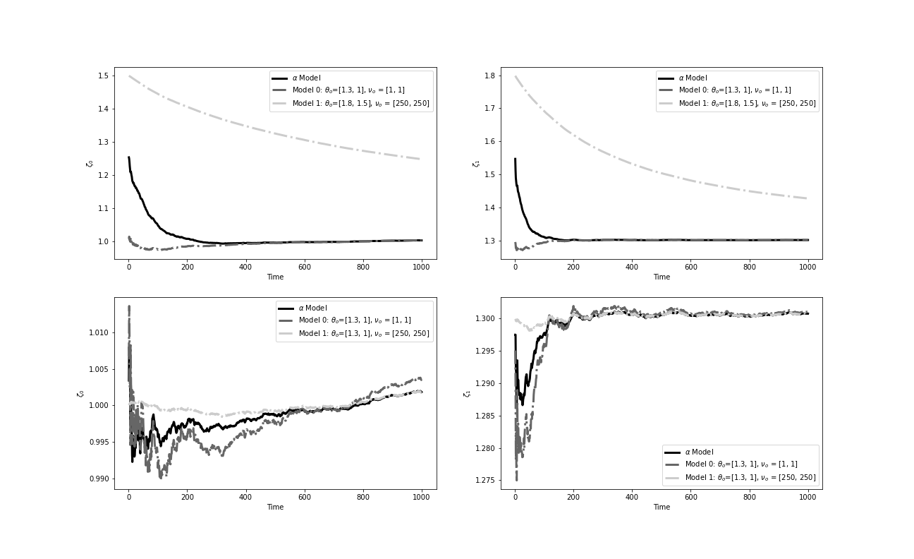
Figure 3: Posterior Beliefs Over Time, Holding Behavior Constant

An important feature of how we aggregate across models is that it generates a robustness property. Because $\alpha_{t}^{o}(d)$ will place less weight on models that are not externally valid, over time they will have limited influence on the PM’s beliefs and consequent decisions. We illustrate this Figure 3. In the top graphs, we plot the policymaker’s posterior beliefs about the mean of the potential outcome distributions over time. The plot distinguishes between three posterior means. The bottom (dashed) line corresponds to one set of priors, which we assume to be unbiased (i.e. $\zeta^{o}_{o}=\theta$), but diffuse. The top (dash-dotted) line refers to an alternative set of priors, which contains some degree of stubbornness (i.e. $\zeta^{o}_{o}=\theta+.5,\nu=250$). The middle (solid) line comes from the combined model, which is a weighted average of the two sets of priors using $\alpha_{t}^{o}(d)$ as weights. We see that even though our policymaker starts with a stubborn prior, the combined model converges relatively quickly to the non-stubborn model. This is the result of both the oracle property – concentrating on the least stubborn model – and robustness property – putting less and less weight on sufficiently stubborn models.

In the bottom graphs, we consider the case in which the alternative model is confident. Thus, both sets of priors are unbiased; the alternative prior simply comes with a higher degree of conviction. Because both priors are correct, the combined model does not immediate converge to one of the models as we saw in case with stubborn priors. As we started in Lemma B.1, our parameter $\alpha$ is more responsive to bias than conviction.

Concentration Bounds

Effects of $\epsilon$.

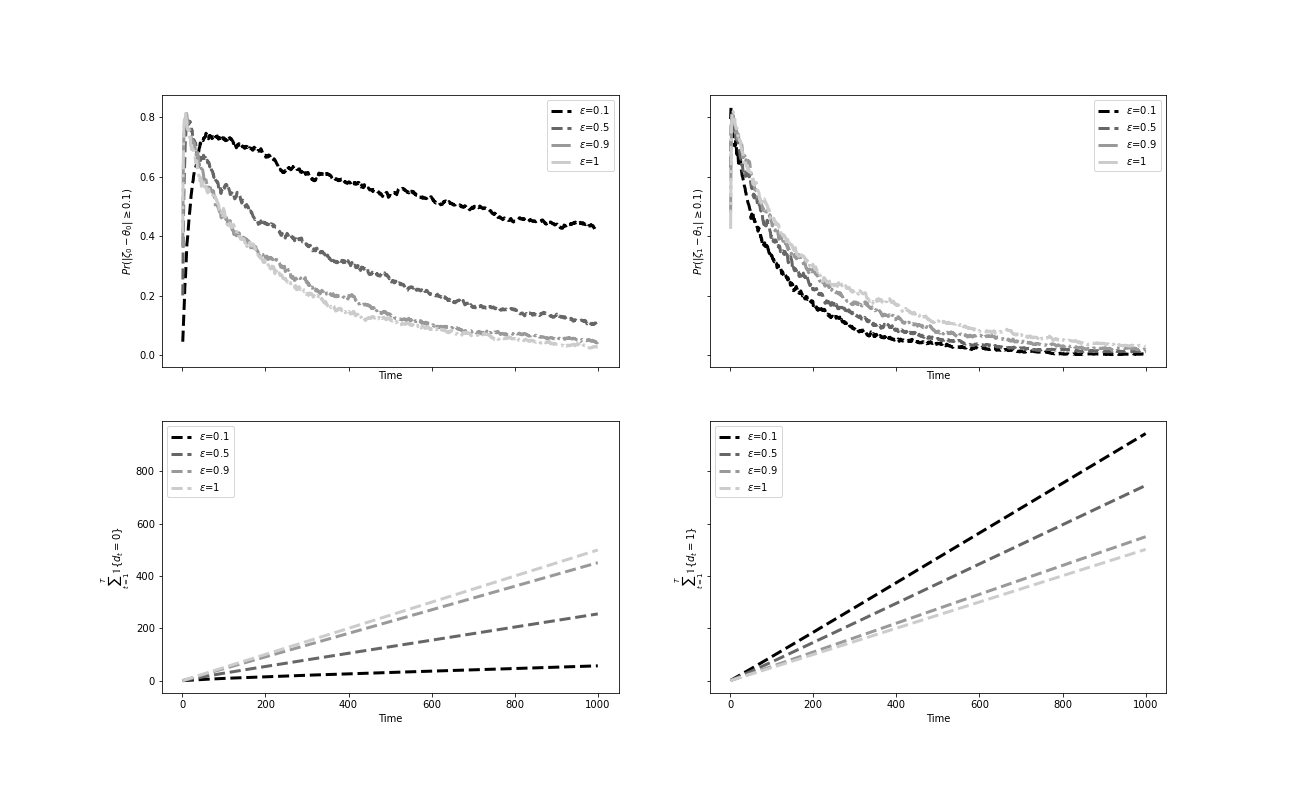
Figure 4: Concentration Bounds and Frequency of Play

We now simulate our model’s concentration bounds and some its key properties. Recall from Remark 3.1 in Section 3.1, the concentration rate increases with the parameter $\epsilon$. We demonstrate this property in the top panel of Figure 4, in which we plot concentration bounds for three different values of $\epsilon\in\{0.1,0.5,0.9\}$. That is, for a given $\epsilon$, we compute the difference over time between the policymaker’s posterior belief of the true mean, $\zeta^{o}_{t}(d)$, and the true mean, $\theta(d)$. We then plot the probability that these differences are greater than 0.1. For these simulations, we assume that our policymaker has correct, but diffuse priors (i.e. $\zeta^{o}_{0}=\theta$ and $\nu^{o}_{0}=[1,1]$).

In the top panel, we see that except for early on, our concentration bounds decrease over time and in the case of $\zeta^{o}_{t}(0)$ decrease faster, the higher the $\epsilon$. For instance, after 1000 instances, $Pr(\zeta^{o}_{t}(0)-\theta(0)>0.1)$ is almost zero for the case of $\epsilon=0.9$, but is still close to 0.5 for $\epsilon=0.1$. For the other treatment arm, the patterns are reversed. All three lines decrease relatively quickly, with the lower $\epsilon$ lines decreasing faster.

The intuition for these patterns is straightforward and speaks to the point about frequency of play in Remark 3.1. When the PM selects a treatment arm, she will only learn about the distribution of potential outcomes for that arm. As she become more confident in which arm is better, she will play the other arm only when forced to by the $\epsilon$-greedy algorithm. In this case, the higher the $\epsilon$ the more the PM will be forced to play treatment $d=0$ and the more she learns about $\theta(0)$. We can see this clearly in the bottom panel, which depicts the cumulative number of times the treatment has been played over time by different values of $\epsilon$’s. As we compare the two panels, the more we play a particular arm, the more we learn about it, and the sooner our beliefs converge to the truth.

Effects of Priors.

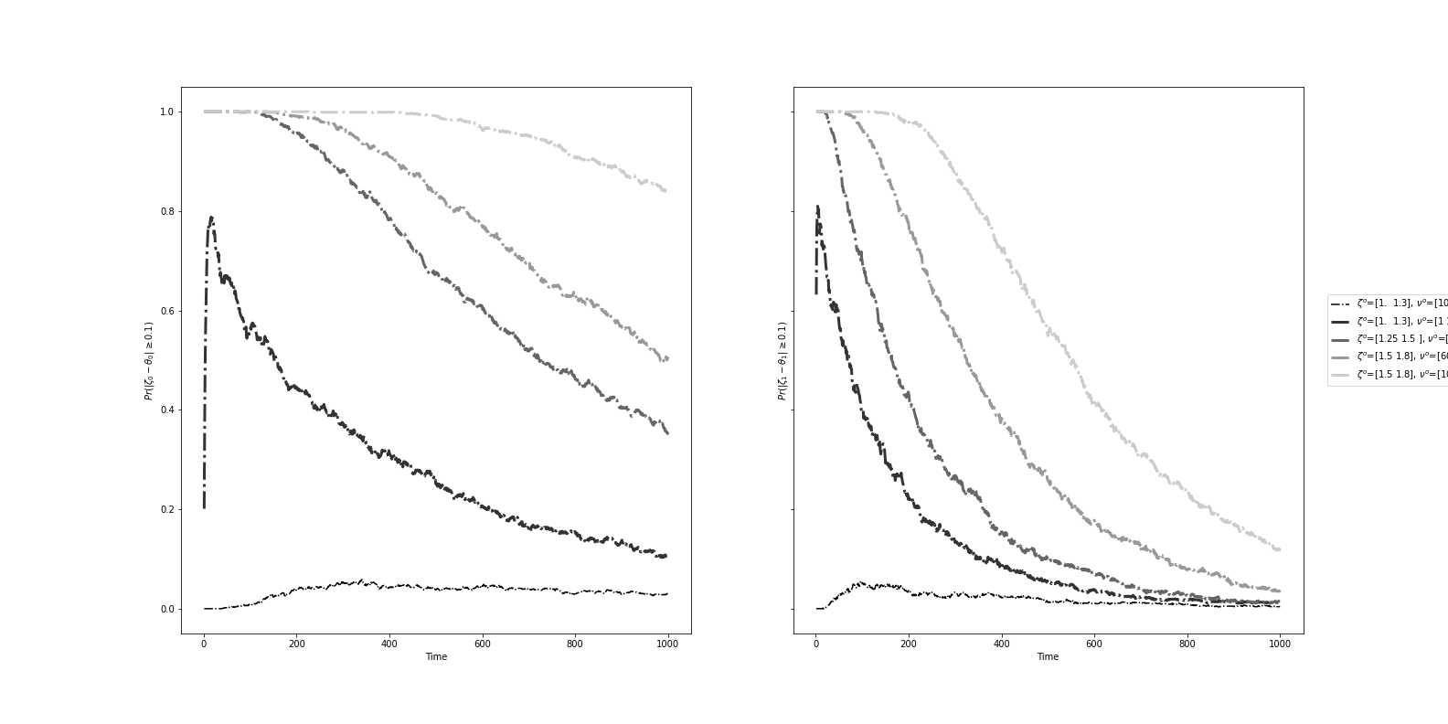
Figure 5: Concentration Bounds by Model Stubbornness

In Figure 5, we investigate the effects of different priors on the concentration bounds. In particular, we plot different concentration bounds for priors with different degrees of stubbornness and confidence. For example, in the bottom two lines, we consider two unbiased priors, but with different levels of confidence. According to Remark 3.1, concentration rates increase as the degree of conviction increases and this precisely what we see. It is also the case, that the concentration rate decreases faster with less stubborn models. We can see this pattern clearly by comparing the top two lines. By comparing the two middle lines, we can also see that conditional on the degree of stubbornness, the higher the bias, the slower the concentration rate. Lastly, the concentration rates for $\theta(1)$ tend to be faster than those for $\theta(0)$ because of the frequency of play.

Probability of Making a Mistake

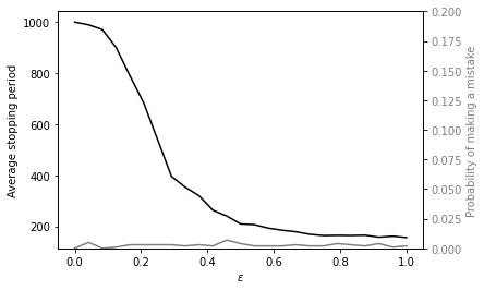
Figure 6: Stopping Period and Probability of Making a Mistake

In Section 3.2, we defined a mistake as recommending a treatment arm different from the one that yields the largest expected effect at the instance in which the experiment was stopped. In Figure 6, we plot the average stopping period (left axis) and the probability of making a mistake at that stopping period (right axis) by $\epsilon$. It is clear from the graph that the more we experiment across treatment arms (i.e., higher $\epsilon$), the faster we stop the experiment. This makes sense. As we experiment more, the data become more IID and we are able to better learn the true means of the potential outcome distributions. According to these simulations, the degree of experimentation does not have to be particularly high. Even though at low levels of $\epsilon$ the experiment lasts for almost its entire duration, the drop off is fairly quick. Once $\epsilon$ is greater than 0.5, the difference gained in stopping periods from additional experimentation is minimal.

Shorter stopping periods do not come at the cost of making more mistakes. This result is to some extent an artifact of our stopping rule, whose parameters control the probability of type I errors. As the graph depicts, the probability of making a mistake varies little with $\epsilon$ and is always below 1%.

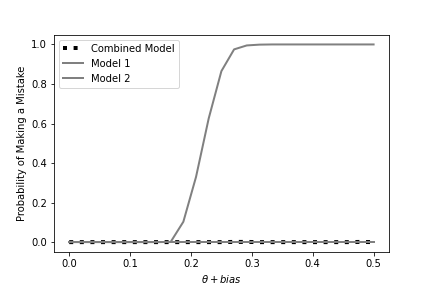
Figure 7: Probability of Making a Mistake by Model Bias

In Figure 7, we explore how the initial priors affect the probability of making a mistake. We again consider two sets of priors, both with $\nu_{0}=[250,250]$. One, however, is confident with $\zeta^{o}_{0}=\theta$, whereas the other is stubborn, with $\zeta^{o}_{0}=[\theta(0)+\delta,\theta(1)-\delta]$, where $\delta$ is indicated by a point on the x-axis. For $\delta\in(0,0.15)$, the priors are biased, but have a proper ranking of the treatment arms. For $\delta>0.15$, the priors are not only biased, but reverse the ranking of the arms. On the y-axis, we plot the probability of making a mistake associated with each set of priors, as well as for the combined model.

We can see that for $\delta\in(0,0.15)$, the probability of making mistake is small, less than 1%, for all three models. But once $\delta>0.15$, and the ranking of treatment arms are reversed, the probability of making a mistake for the stubborn model increases significantly and approaches 1 by $\delta\geq 0.3$. Importantly, the probability of making a mistake for the combined model mirrors the one for the confident model, which again illustrates the robustness property of $\alpha^{o}_{t}(d)$.

Expected Earnings

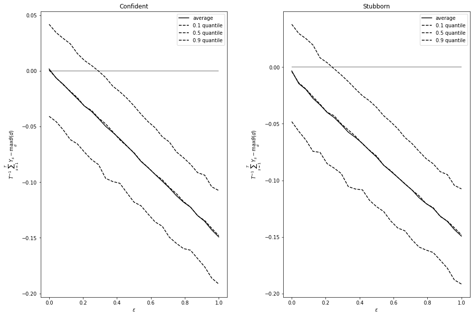
Figure 8: Relative Average Earnings During the Experiment

The final outcome we evaluate is expected earnings. According to Proposition 3.3, the distance between the average outcomes and maximum expected outcome is decreasing in $\epsilon$. In Figure 8, we plot by $\epsilon$, the difference between the policymaker’s average impact and the maximum expected outcome, $\max_{d}\theta(d)$, for an experiment that lasts 1000 instances. The figure also distinguishes between our two familiar sets of priors, a confident one and a stubborn one.

Two important observations emerge from this figure. First, there is a steep negative monotonic relationship between expected earning and $\epsilon$. In fact, the 10% quantile of the average earnings distribution for $\epsilon=0.10$ lies above the 90% quantile of the average earnings distribution for $\epsilon=0.90$. Second, if we compare across the two plots, we can see that starting off with a stubborn prior affects average earnings, but only minimally. Again, this result is a product of the robustness property that our model aggregation approach provides.

The fact that average earnings declines with experimentation does not imply that our policymaker should set $\epsilon$ close to zero. Because as we saw in Figure 6, lower $\epsilon$’s result in longer experiments, which can come with costs. Moreover, as we show in Proposition 3.2, the upper bound the probability of making a mistake is weakly smaller for higher levels of $\epsilon$. Thus, to properly capture the experimentation versus exploitation tradeoff inherent in multi-armed bandit problems, we need to specify a payoff function.

We consider the following payoff function:

$$\Pi^{I}_{\beta,c}= \sum_{d=0}^{M}\sum_{t=0}^{T^{\ast}}\beta^{t}1\{D_{t}=d\}(Y_{t}(d)-c_{1})+\sum_{t=T^{\ast}+1}^{\infty}\beta^{t}1\{D_{T^{\ast}}=d\}(\theta(d)-c_{2})$$ (4.1)

$$= \sum_{d=0}^{M}\sum_{t=0}^{T^{\ast}}\beta^{t}1\{D_{t}=d\}(Y_{t}(d)-c_{1})+\frac{\beta^{T^{\ast}+1}}{1-\beta}1\{D_{T^{\ast}}=d\}(\theta(d)-c_{2})$$ (4.2)

where $c_{1}$ indicates the costs of running the experiment, $c_{2}$ cost of administering the treatment, $\beta^{t}$ represents a discount factor, and $T^{\ast}$ denotes the stopping period. This payoff function comprises of two parts. The first part is the earnings during the experiment net of cost. The second part captures the expected future benefits under the chosen treatment, net of cost.

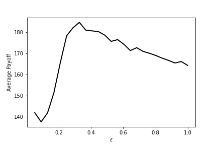
Figure 9: Experimentation versus Exploitation – Expected Payoffs

In Figure 9, we compute the payoff function for our model simulations by different values of $\epsilon$. In contrast with the previous figure, we see that the average payoffs are increasing with $\epsilon$ until approximately $\epsilon=0.38$, at which point the payoffs start to decline. While this “optimal” value of $\epsilon$ is clearly a function of an arbitrary set of parameter choices, our conjecture is that the inverted u-shape relationship is likely to hold more generally, suggesting that some combination of experimentation and exploitation is optimal.

5 Charitable Fundraising Experiment

In this section, we present a real-world numerical example to show that by incorporating multiple priors, our policymaker can stop the experiment sooner without significantly increasing the probability of making a mistake. This results in large performance gains relative to a standard RCT.

Our numerical example uses data from a direct mail fundraising experiment reported in Karlan and List, (2020). The experiment, which we will refer to as the BMGF experiment, consisted of sending 51,971 solicitation letters to previous donors of a charity focused on international development and poverty reduction. Donors were randomly assigned to receive letters with or without information about a $2:$1 limited-time matching grant offered by the Bill and Melinda Gates Foundation. Letters were mailed in December 2009 and responses were tracked until March 2011.

The authors find that a matching grant from the Bill and Melinda Gates Foundation was effective at increasing donations. Over the course of the experiment, the treatment increased the total unconditional amount given by $0.36 relative to a control mean of $0.26, an increase of 38%.

We use the data from this experiment to conduct a series of Monte Carlo simulations. We chose this experiment for two reasons. First, charitable giving is an outcome that responds relatively quickly to treatment: conditional on donating, letter recipients will typically respond within a month. Second, and more importantly for our setup, similar experiments have been conducted in various settings, even by the same authors. Thus, we can use the results from these other charitable fundraising experiments as priors when simulating the BMGF experiment.

To run our simulations, we sample from the empirical distributions of the outcomes for the treatment and control groups. We focus on the log amount given during the experiment conditional on donating. In the treatment group, 225 individuals gave a donation, at an average log amount of 3.56. In the control group, 121 individuals donated, resulting in an average log amount of 3.34. Given these two empirical distributions, we simulate our model 1000 times for 600 instances, which is the minimum number of observations needed for the average difference between treatment and control to become statistically significant.

Our simulations incorporate five sets of priors. The first two sets of priors come from an experiment that Karlan and List, (2020) ran in conjunction with the BMGF experiment, but for a different population of donors. The experimental arms were also different in that both treatment and control were offered a $2:$1 limited-time matching grant. The treatment group, however, was told that the Bill and Melinda Gates Foundation was the matching donor, whereas this information was kept anonymous for the control group. This treatment led to 16.6% (robust standard error = 0.099) increase in donations conditional on giving. We generate two different priors from this experiment that differ in their level of confidence. We set the first prior to $\zeta_{0}=[3.11,3.27],\nu_{0}=[284,223]$, where the $\nu_{0}$ reflects the number of treated in each arm. We set the second prior to $\zeta_{0}=[3.11,3.27],\nu_{0}=[0.01,0.01]$, which makes the prior diffuse. By introducing a diffuse version of this prior, we allow the policymaker to reject priors that are overly stubborn sooner.

The second set of priors comes from another fundraising experiment that the authors conducted in 2005 (Karlan and List,, 2007). Similar to the BMGF experiment, this experiment also offered, as one of its treatment, a $2:$1 limited-time matching grant relative to a no-matching grant control. However, both the organization requesting the donation and the pool of donors were likely quite different. In this case, the treatment effect only led to 1.5% increase in donations conditional on giving. As before, we generate two other sets of priors from this experiment that again only differ in their level of confidence. We set the first prior to $\zeta_{0}=[3.42,3.44],\nu_{0}=[782,252]$, where the $\nu_{0}$ reflects the number of treated in each arm. We set the second prior to $\zeta_{0}=[3.42,3.44],\nu_{0}=[0.01,0.01]$, which makes the prior diffuse. The last set of priors is completely diffuse. We set $\zeta_{0}=[0,0],\nu_{0}=[0.01,0.01]$.

We present the results of the simulation in Table 1. In column 1, we present the results from simulating the RCT for 600 periods. In columns 2-5, we display the results from simulating our model with multiple priors. We present our model for several values of $\epsilon$ to assess the robustness of the findings to different degrees of exploration. In columns 6-10, we again report simulation results for different values of $\epsilon$, but for a model that does not incorporate the use of priors.

The average stopping period of our multi-prior model is less than 200 periods, across each $\epsilon$. This is much lower than the stopping period of the standard RCT (by construction), as well as of the non multi-prior models, which average around 525 instances across the various $\epsilon$. Importantly, the shorter stopping periods of our multi-prior models do not come with a substantial increase in the probability of making a mistake, which is less than 3 percent across the different $\epsilon$.

One of the main advantages of our model, relative to the RCT, can be seen when comparing the average cumulative payoff distributions. We define the cumulative payoff as the sum of donations received at each instance over the 600 periods. At each instance, the policymaker receives a donation amount depending on which treatment was selected. In cases in which the experiment was stopped, the policymaker received the average payoff of the potential outcomes distribution corresponding to her selected treatment.

When comparing cumulative payoffs, our model outperforms the RCT by a wide margin. The $90^{th}$ percentile of the payoff distribution of the RCT is lower than the even the $10^{th}$ percentile of our multi-prior model. In fact, the maximum the policymaker could achieve (should she always choose treatment) is 2136 on average. Our framework achieves 99% of this maximum.

Our multi-prior models also outperform the models without priors, but only minimally. This is not too surprising since these models are also adaptive and thus, engages in a fair amount of exploitation. Nevertheless, it is worth highlighting that we are only comparing payoffs. If there were important costs associated with running longer experiments (as is usually the case) then in terms of net payoffs, our multi-prior model would outperform the models without priors to a much larger extent.

In Table 2, we report our measure of external validity associated with each of the initial priors for the model with $\epsilon=0.3$. On the basis of average outcomes, the least biased model is the experiment from Karlan and List, (2007). Our measure assigns a weight of 0.646 for $\theta_{0}$ and 0.869 for $\theta_{1}$. The $\alpha$’s are more concentrated for $\theta_{1}$ because that treatment arms has been played more often.

In sum, these simulations provide a proof-of-concept for our model. By incorporating multiple priors, our policymaker not only stopped the experiment sooner, but could do so without risk of making a mistake. When compared to the RCT, this translated into larger performance gains in terms of payoffs.

6 Conclusions

This paper presents a conceptual framework for how to incorporate prior sources of information into the design of a sequential experiment. An obvious issue is how to handle the potential lack of external validity of each of these sources. We address this issue by first presenting a formal definition of external validity that can be used to differentiate sources with different degrees of external invalidity and second, by showing that our framework is robust to including externally-invalid sources. This last property relaxes the burden on the policymaker of having to correctly choose relevant sources of information based on limited ex-ante information. As “stubborn” sources are harder to discard, we believe it is useful to incorporate many priors, including versions that are diffuse.

For the common problem of learning about average treatment effects, we show that our framework offers several nice properties. As we illustrated for the case of charitable giving, these properties translate into substantial gains in performance — such as reducing the duration of experiment and increasing the average payoffs while keeping an acceptable probability of making a mistake — over both standard RCTs and adaptive experiments.

Appendix: Figures & Tables

Notes: This figure plots $\alpha^{0}(d=0,x)$ (left plot) and $\alpha^{0}(d=1,x)$ (right plot) under two alternative sets of priors. For the confident model, the initial priors are: $\zeta^{0}_{0}=\zeta^{1}_{0}=\theta;\nu^{0}_{0}=[1,1];\nu^{1}_{0}=[250,250]$. For the stubborn model, the initial priors are: $\zeta^{0}_{0}=\theta;\zeta^{1}_{0}=\theta+0.3;\nu^{0}_{0}=[1,1];\nu^{1}_{0}=[250,250]$. These figures are based on 1,000 simulations using the following parameters: $\theta=[1,1.3]$, $\epsilon=0.5$.

Notes: This figure plots the policymakers posterior beliefs (i.e. $[\zeta^{o}_{t}(0,x),\zeta^{o}_{t}(1,x)]$) over time, distinguishing between two alternative sets of initial priors. In the top panel, one of the initial priors is stubborn; and in the bottom panel, one of the initial priors is confident. For the stubborn model, the initial priors are: $\zeta^{0}_{0}=\theta;\zeta^{1}_{0}=\theta+0.3;\nu^{0}_{0}=[1,1];\nu^{1}_{0}=[250,250]$. For the confident model, the initial priors are: $\zeta^{0}_{0}=\zeta^{1}_{0}=\theta;\nu^{0}_{0}=[1,1];\nu^{1}_{0}=[250,250]$. These figures are based on 1,000 simulations using the following parameters: $\theta=[1,1.3]$, $\epsilon=0.5$.

Notes: The top panel plots concentration bounds over time for different values of $\epsilon$. The bottom panel plots the number of times the experimental arm was played at time $t$ for different values of $\epsilon$. The graphs on the left correspond treatment arm $d=0$; the graphs on the right correspond to treatment arm $d=1$. These figures are based on 1,000 simulations using the following parameters: $\theta=[1,1.3]$; $\zeta_{0}^{o}=\theta$; $\zeta_{1}^{o}=\theta$; $\nu_{0}^{o}=[1,1]$; $\nu_{1}^{o}=[1,1]$.

Notes: The figure plots concentration bounds over time for different degrees of model stubbornness. The lines in these plots appear in descending order of stubbornness, with the top line being most stubborn and the bottom line being the most confident. The graphs on the left correspond treatment arm $d=0$; the graphs on the right correspond to treatment arm $d=1$. These figures are based on 1,000 simulations using the following parameters: $\theta=[1,1.3]$, $\epsilon=0.5$. The initial priors are specified in the legend.

Notes: This figure plots the average stopping period (left axis) and the probability of making a mistake at the stopping period (right axis) by $\epsilon$. These figures are based on 1,000 simulations using the following parameters: $\theta=[1,1.3]$; $\zeta_{0}^{o}=\theta$; $\zeta_{1}^{o}=\theta$; $\nu_{0}^{o}=[1,1]$; $\nu_{1}^{o}=[1,1]$; $B=100$.

Notes: The figure plots the probability of making a mistake at the stopping period by the degree of bias in model 1’s initial priors. These figures are based on 1,000 simulations using the following parameters: $\theta=[1,1.3]$; $\nu^{0}_{0}=\nu^{1}_{0}=[250,250]$; $\zeta^{0}_{0}=[\theta(0)+bias,\theta(1)-bias]$ ; $\zeta^{1}_{0}=\theta$, $\epsilon=0.5$.

Notes: This figure plots by $\epsilon$, the average earnings net of maximal earnings. These figures are based on 1,000 simulations using the following parameters: $\theta=[1,1.3]$; $\zeta_{0}^{o}=\theta$; $\zeta_{1}^{o}=\theta$; $\nu_{0}^{o}=[1,1]$; $\nu_{1}^{o}=[1,1]$.

Notes: This figure plots by $\epsilon$, the expected payoffs as defined by Equation 4.1. These figures are based on 1,000 simulations using the following parameters: $\theta=[1,1.3]$; $\zeta_{0}^{o}=\theta$; $\zeta_{1}^{o}=\theta$; $\nu_{0}^{o}=[1,1]$; $\nu_{1}^{o}=[1,1]$; $B=100$; $\beta^{t}=0.994$; $c=1.15$; $\lambda=1,100$.

Table 1: Fundraising Matching Grant Experiment

	RCT	$\alpha$-Model				Non-$\alpha$ Model
	(1)	(2)	(3)	(4)	(5)	(6)	(7)	(8)	(9)
$\epsilon$-Greedy	1	0.2	0.25	0.3	0.35	0.2	0.25	0.3	0.35
Average Stopping Period	600	198.3	171.5	180.6	182.4	548.8	527.5	511.6	509.2
Probability of Making a Mistake at Stopping	0.006	0.024	0.027	0.028	0.029	0.033	0.022	0.028	0.022
Average Payoffs	2071.57	2127.94	2127.87	2126.12	2125.46	2117.05	2116.97	2112.32	2111.30
$10^{th}$ Quantile of Payoff Distribution	2032.11	2106.23	2108.70	2104.645	2102.71	2079.99	2080.34	2073.30	2074.08
$50^{th}$ Quantile of Payoff Distribution	2072.69	2131.21	2131.15	2129.36	2129.60	2118.51	2118.63	2114.34	2113.83
$90^{th}$ Quantile of Payoff Distribution	2109.09	2149.75	2149.75	2149.75	2149.75	2153.62	2153.62	2153.62	2153.62

• Notes: This table reports the results of re-simulating the Bill Melinda Gates Foundation Experiment (Karlan and List,, 2020). Each simulation lasted for at most 600 periods, and the results are averaged over 1,000 simulations. In column 1, we report the results for a standard randomized control trial. In columns 2-5, we report the results for several multi-prior models with different degrees of experimentation, as indicated by $\epsilon$. For the multi-prior models, we consider 5 sets of priors, corresponding to: $\zeta^{0}_{0}=[0,0],\nu=[0.01,0.01]$, $\zeta^{1}_{0}=[3.424909,3.4407649],\nu=[782,252]$, $\zeta^{2}_{0}=[3.424909,3.4407649],\nu=[0.01,0.01]$, $\zeta^{3}_{0}=[3.106395,3.2722909],\nu=[284,223]$, $\zeta^{4}_{0}=[3.106395,3.2722909],\nu=[0.01,0.01]$. For the stopping rule, we set $B=100$, In columns 6-10, we report the results for models with different degrees of experimentation, as indicated by $\epsilon$, but no priors.

Table 2: Fundraising Matching Grant Experiment - External Validity

$\theta_{0}=3.34$			$\theta_{1}=3.56$
$\zeta_{0}$	$\nu_{0}$	$\alpha_{0}$	$\zeta_{0}$	$\nu_{0}$	$\alpha_{1}$
0	0.01	0.013	0	0.01	0.038
3.42	782	0.646	3.44	252	0.869
3.42	0.01	0.014	3.44	0.01	0.041
3.11	284	0.313	3.27	223	0.012
3.11	0.01	0.014	3.27	0.01	0.014

• Notes: Notes: This table reports the $\alpha$ corresponding to the initial priors when re-simulating the Bill Melinda Gates Foundation Experiment (Karlan and List,, 2020), with $\epsilon=0.30$. Each simulation lasted for at most 600 periods, and the results are averaged over 1,000 simulations. For the multi-prior models, we consider 5 sets of priors, corresponding to: $\zeta^{0}_{0}=[0,0],\nu=[0.01,0.01]$, $\zeta^{1}_{0}=[3.424909,3.4407649],\nu=[782,252]$, $\zeta^{2}_{0}=[3.424909,3.4407649],\nu=[0.01,0.01]$, $\zeta^{3}_{0}=[3.106395,3.2722909],\nu=[284,223]$, $\zeta^{4}_{0}=[3.106395,3.2722909],\nu=[0.01,0.01]$. For the stopping rule, we set $B=100$.

Online Appendix

Appendix A Notation and some definitions

For any set $S$, let $\Delta(S)$ be the set of Borel probability measures over $S$.

For each $t\in\mathbb{N}$ and each $(d,x)\in\mathbb{D}\times\mathbb{X}$, let $D^{t}(x):=(D_{1}(x),...,D_{t}(x))$, $Y^{t}(x):=(Y_{1}(D_{1}(x),x),...,Y_{t}(D_{t}(x),x))$ and $Y^{t}(d,x):=(Y_{1}(d,x),...,Y_{t}(d,x))$. Let $(Y^{t-1}(x),D^{t-1}(x))\mapsto\delta_{t}(Y^{t-1},D^{t-1})(.|x)\in\Delta(\mathbb{D})$ be the treatment assignment policy rule and $(Y^{t-1}(x),D^{t-1}(x))\mapsto\sigma_{t}(Y^{t-1},D^{t-1})(x)\in[0,1]$ be the stopping policy rule. When there is no risk of confusion we will simply use $\delta_{t}(.|x)$ and $\sigma_{t}(x)$ to denote these rules.

We define the probability measure $\mathbf{P}$ that is used in the probability statements in our proofs. Formally, let $\mathbf{P}$ be a probability measure over histories $((Y^{T}(d,x))_{(d,x)\in\mathbb{D}\times\mathbb{X}},(D^{T}(x))_{x\in\mathbb{X}})$ (and easily extended to infinite histories) constructed as follows: By assumption, for all $(d,x)\in\mathbb{D}\times\mathbb{X}$, $Y_{1}(d,x)$ is IID drawn from $P(.|d,x)$ and $D_{1}(x)\sim\delta_{1}(.|x)$. For any $t>1$, given the past history $((Y^{t-1}(d,x))_{(d,x)\in\mathbb{D}\times\mathbb{X}},(D^{t-1}(x))_{x\in\mathbb{X}})$, with probability $\sigma_{t}(x)$ the experiment is stopped and $D_{t}(x)$ is the same for all subsequent instances; with probability $1-\sigma_{t}(x)$ the experiment is not stopped and $D_{t}(x)\sim\delta_{t}(.|x)$; $Y_{t}(d,x)$ is is IID drawn from $P(.|d,x)$.

For each $(d,x)\in\mathbb{D}\times\mathbb{X}$ and each $t\in\mathbb{N}$, let

$$N_{t}(d,x):=\sum_{s=1}^{t}1\{D_{s}(x)=d\}\leavevmode\nobreak\ and\leavevmode\nobreak\ f_{t}(d,x):=N_{t}(d,x)/t$$ (A.1)

$$\iota_{t}(d,x):=t^{-1}\sum_{s=1}^{t}\delta_{s}(d|x)$$ (A.2)

$$J_{t}(d,x):=t^{-1}\sum_{s=1}^{t}1\{D_{s}(x)=d\}Y_{s}(d,x).$$ (A.3)

Appendix B Proof of Proposition 2.1

The proof of the proposition uses the following lemma

Lemma B.1.

Let $p_{\theta}$ denote a Gaussian PDF with mean $\theta$ and variance $1$. Then, for any $(d,x)\in\mathbb{D}\times\mathbb{X}$ and any $t\geq 1$,

$$\alpha^{o}_{t}(d,x)=\frac{\phi(m_{t}(d,x);\zeta^{o}_{0}(d,x),(N_{t}(d,x)+\nu^{o}_{0}(d,x))/(N_{t}(d,x)\nu^{o}_{0}(d,x)))}{\sum_{o=0}^{L}\phi(m_{t}(d,x);\zeta^{o}_{0}(d,x),(N_{t}(d,x)+\nu^{o}_{0}(d,x))/(N_{t}(d,x)\nu^{o}_{0}(d,x)))},$$

where $m_{t}(d,x):=\sum_{s=1}^{t}1\{D_{s}(x)=d\}Y_{s}(d,x)/\sum_{s=1}^{t}1\{D_{s}(x)=d\}$.

Proof of Proposition 2.1.

(1) To show this part we note that $\nu^{o}_{0}(d,x)>0$ and thus $\mathbb{EV}_{d,x}(o)\rightarrow-\infty$ iff the bias diverges to plus infinity. From the characterization In Lemma B.1 and the fact that $\phi(m_{t}(d,x);\zeta^{o}_{0}(d,x),(N_{t}(d,x)+\nu^{o}_{0}(d,x))/(N_{t}(d,x)\nu^{o}_{0}(d,x)))=\phi(m_{t}(d,x)-\theta(d,x);\zeta^{o}_{0}(d,x)-\theta(d,x),(N_{t}(d,x)+\nu^{o}_{0}(d,x))/(N_{t}(d,x)\nu^{o}_{0}(d,x)))$ will vanish if the bias diverges to plus infinity, the desired result is obtained.

(2) Observe that

$$\log\phi(m_{t}(d,x);\zeta^{o}_{0}(d,x),(N_{t}(d,x)+\nu^{o}_{0}(d,x))/(N_{t}(d,x)\nu^{o}_{0}(d,x)))$$

$$=C-0.5\log\left((N_{t}(d,x)+\nu^{o}_{0}(d,x))/(N_{t}(d,x)\nu^{o}_{0}(d,x))\right)-0.5\frac{\left(m_{t}(d,x)-\zeta^{o}_{0}(d,x)\right)^{2}}{(N_{t}(d,x)+\nu^{o}_{0}(d,x))/(N_{t}(d,x)\nu^{o}_{0}(d,x))}$$

where $C$ is some universal constant.

If $\inf_{t}t^{-1}\sum_{s=1}^{t}\delta_{s}(d|x)>0$, by LLN $N_{t}(d,x)$ will diverge with probability approaching 1 and $m_{t}(d,x)=\theta(d,x)+o_{\mathbf{P}}(1)$. Therefore,

$$\log\phi(m_{t}(d,x);\zeta^{o}_{0}(d,x),(N_{t}(d,x)+\nu^{o}_{0}(d,x))/(N_{t}(d,x)\nu^{o}_{0}(d,x)))$$

$$= C-0.5\log\left(1/\nu^{o}_{0}(d,x))\right)-0.5\left(\theta(d,x)-\zeta^{o}_{0}(d,x)\right)^{2}\nu^{o}_{0}(d,x))+o_{\mathbf{P}}(1)$$

$$= C+0.5\mathbb{EV}_{(d,x)}(o)+o_{\mathbf{P}}(1)$$

where the last line follows from the expression in Definition 1. Hence, for any $o\in\{1,...,L\}$,

$$\alpha^{o}_{t}(d,x)=\frac{e^{0.5\mathbb{EV}_{(d,x)}(o)}}{\sum_{o^{\prime}=0}^{L}e^{0.5\mathbb{EV}_{(d,x)}(o^{\prime})}}+o_{\mathbf{P}}(1).$$

Moreover, this expression implies

$$\frac{\alpha^{o^{\prime}}_{t}(d,x)}{\alpha^{o}_{t}(d,x)}=e^{-0.5(\mathbb{EV}_{(d,x)}(o)-\mathbb{EV}_{(d,x)}(o^{\prime}))}+o_{\mathbf{P}}(1).$$

and thus, given definition 2, if $o$ is more externally valid than $o^{\prime}$, $\mathbb{EV}_{(d,x)}(o)-\mathbb{EV}_{(d,x)}(o^{\prime})>0$ so that $\frac{\alpha^{o^{\prime}}_{t}(d,x)}{\alpha^{o}_{t}(d,x)}<1+o_{\mathbf{P}}(1)$. If $o$ is the (only) externally valid source, then according to our definition 2, $\mathbb{EV}_{(d,x)}(o)=\infty$ and with the convention that $c/\infty=0$ for any number $c$, the result follows.

∎

B.1 Proofs of Supplemental Lemmas

Proof of Lemma B.1.

Note that

$$\int\prod_{s=1}^{t}(p_{\theta}(Y_{s}))^{1\{D_{s}(x)=d\}}\mu^{o}_{0}(d,x)(d\theta)$$

$$= \int(2\pi)^{-0.5\sum_{s=1}^{t}1\{D_{s}(x)=d\}}\exp\left\{-\frac{1}{2}\sum_{s=1}^{t}1\{D_{s}(x)=d\}\left(Y_{s}(d,x)-m_{t}(d,x)\right)^{2}\right\}$$

$$\times \exp\left\{-\frac{1}{2}\sum_{s=1}^{t}1\{D_{s}(x)=d\}\left(m_{t}(d,x)-\theta\right)^{2}\right\}$$

$$\times \exp\left\{-\sum_{s=1}^{t}1\{D_{s}(x)=d\}\left(Y_{s}(d,x)-m_{t}(d,x)\right)\left(m_{t}(d,x)-\theta\right)\right\}\phi(\theta;\zeta^{o}_{0}(d,x),1/\nu_{0}^{o}(d,x))d\theta.$$

Observe that

$$\sum_{s=1}^{t}1\{D_{s}(x)=d\}\left(Y_{s}(d,x)-m_{t}(d,x)\right)=0,$$

so, letting $N_{t}(d,x):=\sum_{s=1}^{t}1\{D_{s}(x)=d\}$ it follows that

$$\int\prod_{s=1}^{t}(p_{\theta}(Y_{s}))^{1\{D_{s}(x)=d\}}\mu^{o}_{0}(d,x)(d\theta)= \frac{\exp\left\{-\frac{1}{2}\sum_{s=1}^{t}1\{D_{s}(x)=d\}\left(Y_{s}(d,x)-m_{t}(d,x)\right)^{2}\right\}}{(2\pi)^{0.5\sum_{s=1}^{t}1\{D_{s}(x)=d\}+0.5}N_{t}(d,x)^{0.5}}$$

$$\times \int(2\pi/N_{t}(d,x))^{-1/2}\exp\left\{-\frac{1}{2}\left(m_{t}(d,x)-\theta\right)^{2}N_{t}(d,x)\right\}$$

$$\phi(\theta;\zeta^{o}_{0}(d,x),1/\nu_{0}^{o}(d,x))d\theta.$$

The expression of the integral can be viewed as a convolution between to Gaussian PDFs one indexed by $(0,1/N_{t}(d,x))$ and $(\zeta^{o}_{0}(d,x),1/\nu_{0}^{o}(d,x))$ resp, which in turn is equivalent to PDF of the sum of the corresponding random variables evaluated at $m_{t}(d,x)$. Therefore,

$$\int\prod_{s=1}^{t}(p_{\theta}(Y_{s}))^{1\{D_{s}(x)=d\}}\mu^{o}_{0}(d,x)(d\theta)=C\phi(m_{t}(d,x);\zeta^{o}_{0}(d,x),(N_{t}(d,x)+\nu^{o}_{0}(d,x))/(N_{t}(d,x)\nu^{o}_{0}(d,x)))$$

where $C:=(2\pi)^{-0.5\sum_{s=1}^{t}1\{D_{s}(x)=d\}+0.5}N_{t}(d,x)^{-1/2}\exp\left\{-\frac{1}{2}\sum_{s=1}^{t}1\{D_{s}(x)=d\}\left(Y_{s}(d,x)-m_{t}(d,x)\right)^{2}\right\}$ which, importantly, doesn’t depend on the model $o$.

Hence

$$\alpha^{o}_{t}(d,x)=\frac{\phi(m_{t}(d,x);\zeta^{o}_{0}(d,x),(N_{t}(d,x)+\nu^{o}_{0}(d,x))/(N_{t}(d,x)\nu^{o}_{0}(d,x)))}{\sum_{o=0}^{L}\phi(m_{t}(d,x);\zeta^{o}_{0}(d,x),(N_{t}(d,x)+\nu^{o}_{0}(d,x))/(N_{t}(d,x)\nu^{o}_{0}(d,x)))}$$

and the desired result follows. ∎

Appendix C Non-stochastic Bounds

C.1 Non-stochastic Bounds for $\alpha_{t}$

For each $t\in\{1,...,T\}$ and each $o\in\{1,...,L\}$, let $\overline{\alpha}^{o}_{t}:\mathbb{R}_{+}\times[0,1]\times\mathbb{R}^{1+L}\times\mathbb{N}^{1+L}\rightarrow\mathbb{R}_{+}$ and $\underline{\alpha}^{o}_{t}:\mathbb{R}_{+}\times[0,1]\times\mathbb{R}^{1+L}\times\mathbb{N}^{1+L}\rightarrow\mathbb{R}_{+}$ be defined as follows

$$\overline{\alpha}^{o}_{t}(\delta,g,a,b):=\min\left\{1,\frac{e^{\overline{\ell}_{t}(\delta,g,a^{o},b^{o})}}{\sum_{o^{\prime}=0}^{L}e^{\underline{\ell}_{t}(\delta,g,a^{o^{\prime}},b^{o^{\prime}})}}\right\},\leavevmode\nobreak\ and\leavevmode\nobreak\ \underline{\alpha}^{o}_{t}(\delta,g,a,b):=\frac{e^{\underline{\ell}_{t}(\delta,g,a^{o},b^{o})}}{\sum_{o^{\prime}=0}^{L}e^{\overline{\ell}_{t}(\delta,g,a^{o^{\prime}},b^{o^{\prime}})}}$$

for any $(\delta,g,a,b)\in\mathbb{R}_{+}\times[0,1]\times\mathbb{R}^{1+L}\times\mathbb{N}^{1+L}$, where

$$\overline{\ell}_{t}(\delta,g,a^{o},b^{o}):= -\log\underline{\sigma}_{t}-0.5\frac{\max\{g^{2}(a^{o})^{2}-2\delta a^{o},0\}}{\overline{\sigma}_{t}^{2}}$$

$$\underline{\ell}_{t}(\delta,g,a^{o},b^{o}):= -\log\overline{\sigma}_{t}-0.5\frac{(\delta+a^{o})^{2}}{g^{2}\underline{\sigma}_{t}^{2}}$$

with $(1+b^{o}/T)/b^{o}=:\underline{\sigma}_{t}^{2}\leavevmode\nobreak\ and\leavevmode\nobreak\ (g+b^{o}/t)/(gb)=:\overline{\sigma}_{t}^{2}$.

Lemma C.1.

For any $o\in\{0,...,L\}$, any $t\in\{1,...,T\}$, any $(d,x)\in\mathbb{D}\times\mathbb{X}$ and any $\eta\in(0,h_{t}(d,x))$ and $\delta>0$ such that $f_{t}(d,x)-h_{t}(d,x)\geq-\eta$ and $|J_{t}(d,x)-f_{t}(d,x)\theta(d,x)|\leq\delta$, it follows that

$$\underline{\alpha}^{o}_{t}(\delta,h_{t}(d,x)-\eta,|\bar{\zeta}_{0}(d,x)|,\nu_{0}(d,x))\leq\alpha^{o}_{t}(d,x)\leq\overline{\alpha}^{o}_{t}(\delta,h_{t}(d,x)-\eta,|\bar{\zeta}_{0}(d,x)|,\nu_{0}(d,x)).$$

Proof of Lemma C.1 .

By Lemma B.1 it suffices to bound $\phi(J_{t}(d,x)/f_{t}(d,x);\zeta^{o}_{0}(d,x),(N_{t}(d,x)+\nu^{o}_{0}(d,x))/(N_{t}(d,x)\nu^{o}_{0}(d,x)))$. To do this, note that

$$\phi(J_{t}(d,x)/f_{t}(d,x);\zeta^{o}_{0}(d,x),(N_{t}(d,x)+\nu^{o}_{0}(d,x))/(N_{t}(d,x)\nu^{o}_{0}(d,x)))$$

$$=\frac{\sqrt{(N_{t}(d,x)\nu^{o}_{0}(d,x))}}{2\pi\sqrt{(N_{t}(d,x)+\nu^{o}_{0}(d,x))}}\exp\left\{-0.5\frac{\left(J_{t}(d,x)-f_{t}(d,x)\zeta^{o}_{0}(d,x)\right)^{2}}{f_{t}(d,x)}\frac{N_{t}(d,x)\nu^{o}_{0}(d,x)}{f_{t}(d,x)(N_{t}(d,x)+\nu^{o}_{0}(d,x))}\right\}$$

$$=\frac{\sqrt{f_{t}(d,x)\nu^{o}_{0}(d,x)}}{2\pi\sqrt{(f_{t}(d,x)+\nu^{o}_{0}(d,x)/t)}}\exp\left\{-0.5\frac{\left(\bar{J}_{t}(d,x)-f_{t}(d,x)\bar{\zeta}^{o}_{0}(d,x)\right)^{2}}{f_{t}(d,x)}\frac{\nu^{o}_{0}(d,x)}{(f_{t}(d,x)+\nu^{o}_{0}(d,x)/t)}\right\}$$

where $\bar{.}$ indicates centered at $\theta(d,x)$. Henceforth, let $\sigma^{2}_{t}:=(f_{t}(d,x)+\nu^{o}_{0}(d,x)/t)/(f_{t}(d,x)\nu^{o}_{0}(d,x))$.

Under $|\bar{J}_{t}(d,x)|\leq\delta$, if follows that

$$(\bar{J}_{t}(d,x)-f_{t}(d,x)\bar{\zeta}^{o}_{0}(d,x))^{2}= (\bar{J}_{t}(d,x))^{2}+(f_{t}(d,x)\bar{\zeta}^{o}_{0}(d,x))^{2}-2\bar{J}_{t}(d,x)f_{t}(d,x)\bar{\zeta}^{o}_{0}(d,x)$$

$$\leq \delta^{2}+(f_{t}(d,x)\bar{\zeta}^{o}_{0}(d,x))^{2}+2\delta f_{t}(d,x)|\bar{\zeta}^{o}_{0}(d,x)|$$

$$\leq (\delta+|\bar{\zeta}^{o}_{0}(d,x)|)^{2}$$

and, in addition, if $f_{t}(d,x)-h_{t}(d,x)\geq-\eta$ with $\eta\leq h_{t}(d,x)$, then

$$(\bar{J}_{t}(d,x)-f_{t}(d,x)\bar{\zeta}^{o}_{0}(d,x))^{2}= (\bar{J}_{t}(d,x))^{2}+(f_{t}(d,x)\bar{\zeta}^{o}_{0}(d,x))^{2}-2\bar{J}_{t}(d,x)f_{t}(d,x)\bar{\zeta}^{o}_{0}(d,x)$$

$$\geq (f_{t}(d,x)\bar{\zeta}^{o}_{0}(d,x))^{2}-2f_{t}(d,x)\delta|\bar{\zeta}^{o}_{0}(d,x)|$$

$$\geq (h_{t}(d,x)-\eta))^{2}(\bar{\zeta}^{o}_{0}(d,x))^{2}-2\delta|\bar{\zeta}^{o}_{0}(d,x)|.$$

Also, under these conditions,

$$\sigma^{2}_{t}\geq (1+\nu^{o}_{0}(d,x)/t)/(\nu^{o}_{0}(d,x))\geq(1+\nu^{o}_{0}(d,x)/T)/(\nu^{o}_{0}(d,x))=:\underline{\sigma}_{t}^{2}$$

$$\leq (h_{t}(d,x)-\eta+\nu^{o}_{0}(d,x)/t)/((h_{t}(d,x)-\eta)\nu^{o}_{0}(d,x))=:\overline{\sigma}_{t}^{2}.$$

Therefore,

$$\log\phi(\bar{m}_{t}(d,x)-\bar{\zeta}^{o}_{0}(d,x);0,\sigma^{2}_{t}(d,x))\geq -\log\sigma_{t}-0.5\frac{(\delta+|\bar{\zeta}^{o}_{0}(d,x)|)^{2}}{f_{t}(d,x)^{2}\sigma^{2}_{t}}+Cte\geq-\log\overline{\sigma}_{t}-0.5\frac{(\delta+|\bar{\zeta}^{o}_{0}(d,x)|)^{2}}{(h_{t}(d,x)-\eta)^{2}\underline{\sigma}_{t}^{2}}+Cte$$

$$=: \underline{\ell}_{t}(\delta,h_{t}(d,x)-\eta,|\bar{\zeta}^{o}_{0}(d,x)|,\nu_{0}^{o}(d,x))+Cte$$

and

$$\log\phi(\bar{m}_{t}(d,x)-\bar{\zeta}^{o}_{0}(d,x);0,\sigma^{2}_{t}(d,x))\leq -\log\sigma_{t}-0.5\frac{\max\{(h_{t}(d,x)-\eta))^{2}(\bar{\zeta}^{o}_{0}(d,x))^{2}-2\delta|\bar{\zeta}^{o}_{0}(d,x)|,0\}}{f_{t}(d,x)^{2}\sigma^{2}_{t}}+Cte$$

$$\leq -\log\underline{\sigma}_{t}-0.5\frac{\max\{(h_{t}(d,x)-\eta))^{2}(\bar{\zeta}^{o}_{0}(d,x))^{2}-2\delta|\bar{\zeta}^{o}_{0}(d,x)|,0\}}{\overline{\sigma}_{t}^{2}}+Cte$$

$$=: \overline{\ell}_{t}(\delta,h_{t}(d,x)-\eta,|\bar{\zeta}^{o}_{0}(d,x)|,\nu_{0}^{o}(d,x)).$$

∎

Lemma C.2.

The following properties are true:

1. $\delta\mapsto\underline{\ell}_{t}(\delta,g,|\bar{\zeta}^{o}_{0}(d,x)|,\nu_{0}^{o}(d,x))$ is decreasing and $\delta\mapsto\overline{\ell}_{t}(\delta,g,|\bar{\zeta}^{o}_{0}(d,x)|,\nu_{0}^{o}(d,x))$ is non-decreasing.

2. $g\mapsto\underline{\ell}_{t}(\delta,g,|\bar{\zeta}^{o}_{0}(d,x)|,\nu_{0}^{o}(d,x))$ is increasing and $g\mapsto\overline{\ell}_{t}(\delta,g,|\bar{\zeta}^{o}_{0}(d,x)|,\nu_{0}^{o}(d,x))$ is decreasing.

3. $\delta\mapsto\overline{\alpha}^{o}_{t}(\delta,g,|\zeta_{0}(d,x)|,\nu_{0}(d,x))$ is increasing and $\delta\mapsto\overline{\alpha}^{o}_{t}(\delta,g,|\zeta_{0}(d,x)|,\nu_{0}(d,x))$ is decreasing.

4. $g\mapsto\overline{\alpha}^{o}_{t}(\delta,g,|\zeta_{0}(d,x)|,\nu_{0}(d,x))$ is decreasing and $g\mapsto\underline{\alpha}^{o}_{t}(\delta,g,|\zeta_{0}(d,x)|,\nu_{0}(d,x))$ is increasing.

5. $t\mapsto\overline{\alpha}^{o}_{t}(\delta,g,|\zeta_{0}(d,x)|,\nu_{0}(d,x))$ is increasing and $t\mapsto\underline{\alpha}^{o}_{t}(\delta,g,|\zeta_{0}(d,x)|,\nu_{0}(d,x))$ is decreasing.

Proof of Lemma C.2.

(1) It is easy to see that $\underline{\ell}_{t}(\delta,g,|\bar{\zeta}^{o}_{0}(d,x)|,\nu_{0}^{o}(d,x),h_{t}(d,x))$ is decreasing in $\delta$ and $\overline{\ell}_{t}(\delta,g,|\bar{\zeta}^{o}_{0}(d,x)|,\nu_{0}^{o}(d,x))$ is non-decreasing in $\delta$.

(2) We first observe that $\underline{\sigma}^{2}_{t}$ is constant as a function of $g=h_{t}(d,x)-\eta$ and $\overline{\sigma}^{2}_{t}$ is an decreasing function of $g:=h_{t}(d,x)-\eta$. Also, note that $\frac{d\underline{\ell}_{t}(\delta,g,|\bar{\zeta}^{o}_{0}(d,x)|,\nu_{0}^{o}(d,x))}{dg}=-\frac{1}{\overline{\sigma}}\frac{d\overline{\sigma}_{t}}{dg}+\frac{(\delta+|\bar{\zeta}^{o}_{0}(d,x)|)^{2}}{(g)^{3}\underline{\sigma}_{t}^{2}}$, thus, since $g\geq 0$, $\underline{\ell}_{t}(\delta,g,|\bar{\zeta}^{o}_{0}(d,x)|,\nu_{0}^{o}(d,x))$ is increasing as a function of $g$. Similarly, $\overline{\ell}_{t}(\delta,g,|\bar{\zeta}^{o}_{0}(d,x)|,\nu_{0}^{o}(d,x))$ is increasing as a function of $\overline{\sigma}^{2}_{t}$ and decreasing as a direct function of $g$, thus by computing the derivative it can be shown that it is decreasing in $g$.

(3-4) By parts (1), it readily follows that $\overline{\alpha}^{o}_{t}(\delta,g,|\zeta_{0}(d,x)|,\nu_{0}(d,x))$ is increasing in $\delta$ and $\underline{\alpha}^{o}_{t}(\delta,g,|\zeta_{0}(d,x)|,\nu_{0}(d,x))$ is decreasing in $\delta$. And by part (2) $\overline{\alpha}^{o}_{t}(\delta,g,|\zeta_{0}(d,x)|,\nu_{0}(d,x))$ is decreasing in $g$ and $\underline{\alpha}^{o}_{t}(\delta,g,|\zeta_{0}(d,x)|,\nu_{0}(d,x))$ is increasing in $g$.

(5) It follows that $t\mapsto\bar{\sigma}^{2}_{t}$ is decreasing and $t\mapsto\underline{\sigma}^{2}_{t}$ is constant. Since $\overline{\ell}_{t}$ is non-increasing in $\bar{\sigma}^{2}_{t}$ it follows that it is non-decreasing in $t$. Similarly, $\underline{\ell}_{t}$ is increasing in $\bar{\sigma}^{2}_{t}$ and thus increasing in $t$.

These results imply that $t\mapsto\overline{\alpha}^{o}_{t}(\delta,g,|\zeta_{0}(d,x)|,\nu_{0}(d,x))$ is increasing and $t\mapsto\underline{\alpha}^{o}_{t}(\delta,g,|\zeta_{0}(d,x)|,\nu_{0}(d,x))$ is decreasing. ∎

C.2 Non-stochastic Bounds for $\zeta^{o}_{t}$

For any $t\in\mathbb{N}$, let $\Omega_{0}:D(\Omega_{0}):=([0,1]\times\mathbb{R}\times\mathbb{N})\rightarrow\mathbb{R}$ and $\Omega:D(\Omega):=\mathbb{R}_{+}\times D(\Omega_{0})\rightarrow\mathbb{R}$ be such that

$$\Omega(\gamma,g,\zeta^{o}_{0}(d,x),\nu^{o}_{0}(d,x)):=\frac{\gamma}{g+\nu^{o}_{0}(d,x)/t}+\Omega_{0}(g,\zeta^{o}_{0}(d,x),\nu^{o}_{0}(d,x))$$

and

$$\Omega_{0}(g,\zeta^{o}_{0}(d,x),\nu^{o}_{0}(d,x)):=\nu^{o}_{0}(d,x)\left(\frac{(\zeta^{o}_{0}(d,x))_{+}/t}{g+\nu^{o}_{0}(d,x)/t}+\frac{(\zeta^{o}_{0}(d,x))_{-}/T}{1+\nu^{o}_{0}(d,x)/t}\right)$$

for any $(\gamma,g,\zeta^{o}_{0}(d,x),\nu^{o}_{0}(d,x))\in D(\Omega)$, where for any real number $a$, $a_{+}:=\max\{a,0\}$ and $a_{-}:=\min\{a,0\}$.

Lemma C.3.

For any $o\in\{0,...,L\}$, any $(d,x)\in\mathbb{D}\times\mathbb{X}$ and any $t\in\mathbb{N}$, the following are true:

1. $\gamma\mapsto\Omega(\gamma,g,\zeta^{o}_{0}(d,x),\nu^{o}_{0}(d,x))$ is increasing.

2. $g\mapsto\Omega(\gamma,g,\zeta^{o}_{0}(d,x),\nu^{o}_{0}(d,x))$ is decreasing and $g\mapsto\Omega_{0}(g,\zeta^{o}_{0}(d,x),\nu^{o}_{0}(d,x))$ is non-increasing.

3. If $\zeta_{0}(d,x)\leq 0$, $\nu_{0}(d,x)\mapsto\Omega(\gamma,g,\zeta^{o}_{0}(d,x),\nu^{o}_{0}(d,x))$ is decreasing; and if $\zeta_{0}(d,x)\leq(\geq)0$ $\nu_{0}(d,x)\mapsto\Omega_{0}(g,\zeta^{o}_{0}(d,x),\nu^{o}_{0}(d,x))$ is non-increasing (non-decreasing).

Proof of Lemma C.3.

(1) Trivial.

(2) By inspection, $g\mapsto\Omega_{0}(g,\zeta^{o}_{0}(d,x),\nu^{o}_{0}(d,x))$ is non-increasing. In addition $g\mapsto\gamma/(g+\nu^{o}_{0}(d,x)/t)$ is decreasing.

(3) Trivial. ∎

Lemma C.4.

For any $o\in\{0,...,L\}$, any $(d,x)\in\mathbb{D}\times\mathbb{X}$ and any $t\in\mathbb{N}$, suppose $f_{t}(d,x)-h_{t}(d,x)\geq-\eta$ for some $\gamma\geq 0$ and $0\leq\eta\leq h_{t}(d,x)\leq\iota_{t}(d,x)$. Then:

1. $|\zeta^{o}_{t}(d,x)-\theta(d,x)|\leq\Omega(\gamma,h_{t}(d,x)-\eta,|\zeta^{o}_{0}(d,x)-\theta(d,x)|,\nu^{o}_{0}(d,x))$.

2. $\zeta^{o}_{t}(d,x)-\theta(d,x)\leq\Omega(\gamma,h_{t}(d,x)-\eta,\zeta^{o}_{0}(d,x)-\theta(d,x),\nu^{o}_{0}(d,x))$.

3. $-(\zeta^{o}_{t}(d,x)-\theta(d,x))\leq\Omega(\gamma,h_{t}(d,x)-\eta,-(\zeta^{o}_{0}(d,x)-\theta(d,x)),\nu^{o}_{0}(d,x))$.

Proof of Lemma C.4 .

(1) Under the conditions, it easy to see that

$$|\zeta^{o}_{t}(d,x)-\theta(d,x)|\leq\frac{\gamma+|\zeta^{o}_{0}(d,x)-\theta(d,x)|\nu^{o}_{0}(d,x)/t}{\iota_{t}(d,x)-\eta+\nu^{o}_{0}(d,x)/t}\leq \frac{\gamma+|\zeta^{o}_{0}(d,x)-\theta(d,x)|\nu^{o}_{0}(d,x)/t}{h_{t}(d,x)-\eta+\nu^{o}_{0}(d,x)/t}$$

$$= \Omega(\gamma,h_{t}(d,x)-\eta,|\zeta^{o}_{0}(d,x)-\theta(d,x)|,\nu^{o}_{0}(d,x)).$$

(2-3) The proof is analogous and thus omitted. ∎

C.3 Non-stochastic Bounds for $\zeta^{\alpha}_{t}$

Let $\Gamma_{0}:D(\Gamma):=\mathbb{R}_{+}\times[0,1]\times\mathbb{R}^{1+L}\times\mathbb{N}^{1+L}\rightarrow\mathbb{R}$ be such that

$$\Gamma_{0}(\gamma,g,\zeta_{0}(d,x),\nu_{0}(d,x)):= \sum_{o=0}^{L}\overline{\alpha}^{o}_{t}(\gamma,g,\zeta_{0}(d,x),\nu_{0}(d,x))\Omega^{+}_{0}(g,\zeta^{o}_{0}(d,x),\nu^{o}_{0}(d,x))$$

$$+\sum_{o=0}^{L}\underline{\alpha}^{o}_{t}(\gamma,g,\zeta_{0}(d,x),\nu_{0}(d,x))\Omega^{-}_{0}(g,\zeta^{o}_{0}(d,x),\nu^{o}_{0}(d,x))$$

where $\Omega^{+}:=\max\{\Omega,0\}$ and $\Omega^{-}:=\min\{\Omega,0\}$, and $\Gamma:D(\Gamma)\rightarrow\mathbb{R}$

$$\Gamma(\gamma,g,\zeta_{0}(d,x),\nu_{0}(d,x)):=\gamma\sum_{o=0}^{L}\frac{\overline{\alpha}^{o}_{t}(\gamma,g,\zeta_{0}(d,x),\nu_{0}(d,x))}{g+\nu^{o}_{0}(d,x)/t}+\Gamma_{0}(\gamma,g,\zeta_{0}(d,x),\nu_{0}(d,x))$$

for any $(\gamma,g,\zeta_{0}(d,x),\nu_{0}(d,x))\in D(\Gamma)$.

Remark C.1.

Another possible formulation for $\Gamma(\gamma,g,\zeta_{0}(d,x),\nu_{0}(d,x))$ is $\max_{o\in\{0,...,L\}}\Omega(\gamma,g,\zeta^{o}_{0}(d,x),\nu^{o}_{0}(d,x))$, so one can define $\Gamma$ as the minimum of this expression and the one above, and depending on the context one can use one bound or the other. The same applies to $\Gamma_{0}$ and $\Omega_{0}$. For the sake of the exposition, however, we do not make this bound explicit. $\triangle$

Lemma C.5.

The following properties are true

1. $\delta\mapsto\Gamma(\delta,g,\zeta_{0}(d,x),\nu_{0}(d,x))$ is increasing and $\delta\mapsto\Gamma(\delta,g,\zeta_{0}(d,x),\nu_{0}(d,x))$ is non-decreasing.

2. $g\mapsto\Gamma(\delta,g,\zeta_{0}(d,x),\nu_{0}(d,x))$ and $g\mapsto\Gamma_{0}(\delta,g,\zeta_{0}(d,x),\nu_{0}(d,x))$ are decreasing.

3. For any positive sequences $(\delta_{t},g_{t})_{t}$, $\Gamma(\delta_{t},g_{t},\zeta_{0}(d,x),\nu_{0}(d,x))=O\left(\frac{\delta_{t}+t^{-1}}{g_{t}+t^{-1}}\right)$ and $\Gamma_{0}(\delta_{t},g_{t},\zeta_{0}(d,x),\nu_{0}(d,x))=O\left(\frac{t^{-1}}{g_{t}+t^{-1}}\right)$.

Proof of Lemma C.5.

(1) (we only establish the results for $\Gamma$ as for $\Gamma_{0}$ is analogous) $\Gamma(\delta,g,\zeta_{0}(d,x),\nu_{0}(d,x))$ is the sum of products

$$\overline{\alpha}^{o}_{t}(\delta,g,|\zeta_{0}(d,x)|,\nu_{0}(d,x))\Omega^{+}(\delta,g,\zeta^{o}_{0}(d,x),\nu^{o}_{0}(d,x))+\underline{\alpha}^{o}(\delta,g,|\zeta_{0}(d,x)|,\nu_{0}(d,x))\Omega^{-}(\delta,g,\zeta^{o}_{0}(d,x),\nu^{o}_{0}(d,x)).$$

Observe that, by Lemma C.2(3), $\overline{\alpha}^{o}_{t}(\delta,g,|\zeta_{0}(d,x)|,\nu_{0}(d,x))$ is increasing as a function of $\delta$ and $\Omega^{+}(\delta,g,\zeta^{o}_{0}(d,x),\nu^{o}_{0}(d,x))$ is non-decreasing as a function of $\delta$ by Lemma C.3(1). Since both quantities are positive, it follows that $\overline{\alpha}^{o}_{t}(\delta,g,|\zeta_{0}(d,x)|,\nu_{0}(d,x))\Omega^{+}(\delta,g,\zeta^{o}_{0}(d,x),\nu^{o}_{0}(d,x))$ is non-decreasing (increasing if $\Omega^{+}(\delta,g,\zeta^{o}_{0}(d,x),\nu^{o}_{0}(d,x))>0$ ). Similarly, by Lemmas C.2(3) and C.3(1), $\underline{\alpha}^{o}_{t}$ is decreasing and $\Omega^{-}$ is non-positive and non-decreasing as a function of $\delta$, so the product is is non-decreasing (increasing if $\Omega^{-}<0$ ). Thus, $\Gamma(\delta,g,\zeta_{0}(d,x),\nu_{0}(d,x))$ is increasing as a function of $\delta$.

(2) (we only establish the results for $\Gamma$ as for $\Gamma_{0}$ is analogous) By a similar argument, Lemma C.3(2) and Lemma C.2(4) it follows that $\Gamma(\delta,g,\zeta_{0}(d,x),\nu_{0}(d,x))$ is decreasing as a function of $g$.

(3) Clearly, $\max_{o\in\{0,...,L\}}\Omega(\delta_{t},g_{t},\zeta_{0}(d,x),\nu_{0}(d,x))=O\left(\frac{\delta_{t}+t^{-1}}{g_{t}+t^{-1}}\right)$. Thus $\Gamma(\delta_{t},g_{t},\zeta_{0}(d,x),\nu_{0}(d,x))$ inherits the same rate. Similarly, $\max_{o\in\{0,...,L\}}\Omega_{0}(g_{t},\zeta_{0}(d,x),\nu_{0}(d,x))=O\left(\frac{t^{-1}}{g_{t}+t^{-1}}\right)$ and $\Gamma_{0}(\delta_{t},g_{t},\zeta_{0}(d,x),\nu_{0}(d,x))$ inherits the same rate. ∎

Lemma C.6.

For any $(d,x)\in\mathbb{D}\times\mathbb{X}$ and any $t\in\mathbb{N}$, suppose $|J_{t}(d,x)-f_{t}(d,x)\theta(d,x)|\leq\gamma$ and $f_{t}(d,x)-h_{t}(d,x)\geq-\eta$ for some $\gamma\geq 0$ and $0\leq\eta\leq h_{t}(d,x)\leq\iota_{t}(d,x)$. Then:

1. $|\zeta^{\alpha}_{t}(d,x)-\theta(d,x)|\leq\Gamma(\gamma,h_{t}(d,x)-\eta,\zeta_{0}(d,x)-\theta(d,x),\nu_{0}(d,x))$.

Proof of Lemma C.6 .

Follows directly from the definition of $\zeta^{\alpha}_{t}$ and Lemmas C.4 and C.1. ∎

C.3.1 Relationship between $\Gamma$ and $\Omega$

For each $o\in\{0,...,L\}$ and $d\in\mathbb{D}$, let $\zeta^{-o}_{0}(d,x)$ be the $L\times 1$ vector of all coordinates of $\zeta_{0}(d,x)$ except for $\zeta^{o}_{0}(d,x)$.

Lemma C.7.

For each $o\in\{0,...,L\}$, $(d,x)\in\mathbb{D}\times\mathbb{X}$, $\gamma,g\geq 0$ and $\nu_{0}(d,x)$,

$$\lim_{\bar{\zeta}^{-o}_{0}(d,x)\rightarrow\infty}\left|\Gamma(\gamma,g,|\zeta_{0}(d,x)|,\nu_{0}(d,x))-\Omega(\gamma,g,|\zeta^{o}_{0}(d,x)|,\nu^{o}_{0}(d,x))\right|=0$$

Proof of Lemma C.7.

By construction of $\overline{\ell}_{t}$ and $\underline{\ell}_{t}$ it is easy to see that for any $o^{\prime}\in\{1,...,L\}$,

$$\lim_{\bar{\zeta}^{o^{\prime}}_{0}(d,x)\rightarrow\infty}\underline{\ell}_{t}(\gamma,g,|\zeta^{o^{\prime}}_{0}(d,x)|,\nu^{o^{\prime}}_{0}(d,x))=\lim_{\bar{\zeta}^{o^{\prime}}_{0}(d,x)\rightarrow\infty}\overline{\ell}_{t}(\gamma,g,|\zeta^{o^{\prime}}_{0}(d,x)|,\nu^{o^{\prime}}_{0}(d,x))=-\infty$$

Moreover, in both cases the rate is $O(-|\zeta^{o^{\prime}}_{0}(d,x)|^{2})$ (observe that the Oh depends on $(\gamma,g,\nu^{o^{\prime}}_{0}(d,x))$ ). Hence, for any $o^{\prime}\neq o$,

$$\underline{\alpha}^{o^{\prime}}_{t}(\gamma,g,|\zeta_{0}(d,x)|,\nu_{0}(d,x))=O(e^{-|\zeta^{o^{\prime}}_{0}(d,x)|^{2}})\leavevmode\nobreak\ and\leavevmode\nobreak\ \overline{\alpha}^{o^{\prime}}_{t}(\gamma,g,|\zeta_{0}(d,x)|,\nu_{0}(d,x))=O(e^{-|\zeta^{o^{\prime}}_{0}(d,x)|^{2}}).$$

That is, they converge to 0 at exponential rate.

On the other hand, $\Omega(\gamma,g,|\zeta^{o^{\prime}}_{0}(d,x)|,\nu^{o^{\prime}}_{0}(d,x))=O(|\zeta^{o^{\prime}}_{0}(d,x)|)$, hence

$$\overline{\alpha}^{o^{\prime}}_{t}(\gamma,g,|\zeta_{0}(d,x)|,\nu_{0}(d,x))\Omega^{+}(\gamma,g,|\zeta^{o^{\prime}}_{0}(d,x)|,\nu^{o^{\prime}}_{0}(d,x))$$

$$+\underline{\alpha}^{o^{\prime}}_{t}(\gamma,g,|\zeta_{0}(d,x)|,\nu_{0}(d,x))\Omega^{-}(\gamma,g,|\zeta^{o^{\prime}}_{0}(d,x)|,\nu^{o^{\prime}}_{0}(d,x))=O(e^{-|\zeta^{o^{\prime}}_{0}(d,x)|^{2}}|\zeta^{o^{\prime}}_{0}(d,x)|)$$

which clearly converges to 0 as $|\zeta^{o^{\prime}}_{0}(d,x)|$ diverges.

On the other hand, these results imply that

$$\lim_{\bar{\zeta}^{-o}_{0}(d,x)\rightarrow\infty}\overline{\alpha}^{o}_{t}(d,x)=\min\left\{1,\frac{e^{\overline{\ell}_{t}\gamma,g,|\zeta^{o}_{0}(d,x)|,\nu^{o}_{0}(d,x))}}{e^{\underline{\ell}_{t}\gamma,g,|\zeta^{o}_{0}(d,x)|,\nu^{o}_{0}(d,x))}}\right\}=1$$

where the last equality follows because $\overline{\ell}_{t}(\gamma,g,|\zeta^{o}_{0}(d,x)|,\nu^{o}_{0}(d,x))\geq\underline{\ell}_{t}(\gamma,g,|\zeta^{o}_{0}(d,x)|,\nu^{o}_{0}(d,x))$.

Therefore $\lim_{\bar{\zeta}^{-o}_{0}(d,x)\rightarrow\infty}\Gamma(\gamma,g,|\zeta_{0}(d,x)|,\nu_{0}(d,x))=\Omega(\gamma,g,|\zeta^{o}_{0}(d,x)|,\nu^{o}_{0}(d,x))$, as desired. ∎

Appendix D Concentration Inequalities

Recall that for any $d\in\{0,...,M\}$ and any $t\geq 0$, let $(h_{t}(d),\omega_{t}(d))\in[0,1]^{2}$ be such that

$$\mathbf{P}\left(\iota_{t}(d)\geq h_{t}(d)\right)\geq 1-\omega_{t}(d),$$

and $\sum_{d=0}^{M}h_{t}(d)=1$, where $\iota_{t}(d):=t^{-1}\sum_{s=1}^{t}\delta_{s}(d)$.

The next lemma presents a Azuma-Hoeffding-type concentration inequality for $(J_{t})_{t}$ and $(f_{t})_{t}$ which are the basis of our theoretical results.

Lemma D.1.

For any $d\in\{0,...,M\}$, any $a\geq 0$ and any $t\geq 0$,

$$\mathbf{P}\left(\left|t^{-1}\sum_{s=1}^{t}(Y_{s}(d)-\theta(d))1\{D_{s}=d\}\right|\geq a\right)\leq 2e^{-0.5t\frac{a^{2}}{\upsilon\sigma(d)^{2}}},$$

and

$$\mathbf{P}\left(\left|t^{-1}\sum_{s=1}^{t}1\{D_{s}=d\}-\iota_{t}(d)\right|\geq a\right)\leq 2e^{-4ta^{2}}.$$

It readily follows that a common bound is given by $2e^{-0.5t\frac{a^{2}}{\max\{1/8,\upsilon\sigma(d)^{2}\}}}$.

Remark D.1 (Remarks on Lemma D.1).

We use Assumption 2(i) in the first part of the lemma. in particular, it is used in order to get an upper bound with exponential decay. The assumption, however, could be replaced by sub-exponential or any other type of control on the MGF of $Y(d)$, e.g., $E[e^{\lambda(Y(d)-\theta(d))}]\leq e^{\kappa(\lambda)}$ for some decreasing function $\lambda\mapsto\kappa(\lambda)$. This change, however, will affect the upper bound obtained in the lemma; it will decay slower than the current one. In fact, up to constant, the result in the lemma will change to

$$\mathbf{P}\left(\left|t^{-1}\sum_{s=1}^{t}(Y_{s}(d)-\theta(d))1\{D_{s}=d\}\right|\geq a\right)\leq 2e^{-t\max_{\lambda\geq 0}\{a\lambda-\kappa(\lambda)\}}.$$

$\triangle$

Proof of Lemma D.1.

Let $W_{s}(d):=(Y_{s}(d)-\theta(d))1\{D_{s}=d\}$. By the Markov inequality, it follows that, for any $\lambda>0$,

$$\mathbf{P}\left(t^{-1}\sum_{s=1}^{t}W_{s}(d)\geq a\right)\leq E\left[\prod_{s=1}^{t}e^{\lambda W_{s}(d)}\right]e^{-a\lambda t}.$$

Observe that

$$E\left[\prod_{s=1}^{t}\exp\{\lambda W_{s}(d)\}\right]=E\left[\prod_{s=1}^{t-1}\exp\{\lambda W_{s}(d)\}E_{t}\left[\exp\{\lambda W_{t}(d)\}\right]\right]$$

where $E_{t}[.]$ denotes the conditional expectation under $\mathbf{P}$ given $(Y_{s})_{s=1}^{t-1}$ and $(D_{s})_{s=1}^{t}$ (but not $Y_{t}(d)$). Observe that $Y_{t}(d)$ is independent of past $Y$’s, given $D_{t}$. This observation and the fact that $Y_{t}(d)$ is sub-gaussian (Assumption 2) imply

$$E_{t}\left[\exp\{\lambda W_{t}(d)\}\right]= E_{t}\left[\exp\{\lambda 1\{D_{t}=d\}(Y_{t}(d)-\theta(d))\}\right]\leq\exp\{0.5\upsilon\sigma(d)^{2}1\{D_{t}=d\}\lambda^{2}\}\leq\exp\{0.5\upsilon\sigma(d)^{2}\lambda^{2}\}.$$

Iterating in this fashion,

$$E\left[\prod_{s=1}^{t}\exp\{\lambda W_{s}(d)\}\right]\leq e^{0.5\upsilon\sigma^{2}(d)\lambda^{2}}E\left[\prod_{s=1}^{t-1}\exp\{\lambda W_{s}(d)\}\right]\leq e^{0.5\upsilon\sigma^{2}(d)t\lambda^{2}}$$

Therefore, for any $\lambda>0$

$$\mathbf{P}\left(t^{-1}\sum_{s=1}^{t}W_{s}(d)\geq a\right)\leq\exp\{0.5\upsilon\sigma^{2}(d)\lambda^{2}t-a\lambda t\}.$$

Choosing $\lambda=a/(\upsilon\sigma^{2}(d))$, it follows that

$$\mathbf{P}\left(t^{-1}\sum_{s=1}^{t}W_{s}(d)\geq a\right)\leq\exp\{-0.5t(a^{2}/(\upsilon\sigma(d)^{2})\}.$$

By analogous calculations, it is easy to show that

$$\mathbf{P}\left(|t^{-1}\sum_{s=1}^{t}W_{s}(d)|\geq a\right)\leq 2\exp\{-0.5t(a^{2}/(\upsilon\sigma(d)^{2})\}.$$

Now let $W_{t}(d):=1\{D_{t}=d\}-\delta_{t}(d)$ and observe that $\left|t^{-1}\sum_{s=1}^{t}W_{s}(d)\right|\geq a$ implies that either $t^{-1}\sum_{s=1}^{t}1\{D_{s}=d\}-\iota_{t}(d)\geq a$ or $(t^{-1}\sum_{s=1}^{t}1\{D_{s}=d\}-\iota_{t}(d))\leq-a$. We only do the proof for the first case since the second one is analogous.

By the Markov inequality, it follows that, for any $\lambda>0$,

$$\mathbf{P}\left(t^{-1}\sum_{s=1}^{t}W_{s}(d)\geq a\right)= E\left[1\{t^{-1}\sum_{s=1}^{t}W_{s}(d)\geq a\}\right]\leq e^{-\lambda at}E\left[\prod_{s=1}^{t}e^{\lambda W_{s}(d)}\right]=e^{-\lambda at}E\left[\prod_{s=1}^{t-1}e^{\lambda W_{s}(d)}E_{t-1}[e^{\lambda W_{t}(d)}]\right]$$

where the last line follows by LIE, where $E_{t-1}$ is the expectation conditional on $(Y^{t-1},D^{t-1})$.

Given $(Y^{t-1},D^{t-1})$, $\delta_{t}(.)$ is non-random as it is measurable with respect to these variables. Thus,

$$E_{t-1}\left[e^{\lambda W_{t}(d)}\right]=e^{-\lambda\delta_{t}(d)}\left(\delta_{t}(d)e^{\lambda}+(1-\delta_{t}(d))\right)=e^{L(\lambda)}$$

where $L(\lambda)=-\lambda\delta_{t}(d)+\log\left(\delta_{t}(d)e^{\lambda}+(1-\delta_{t}(d))\right)$. Observe that $L(0)=0$, $L^{\prime}(\lambda)=-\delta_{t}(d)+\delta_{t}(d)\frac{e^{\lambda}}{\delta_{t}(d)e^{\lambda}+(1-\delta_{t}(d))}$ so that $L^{\prime}(0)=0$ and $L^{\prime\prime}(\lambda)=\delta_{t}(d)\left(\frac{e^{\lambda}(1-\delta_{t}(d))}{(\delta_{t}(d)e^{\lambda}+(1-\delta_{t}(d)))^{2}}\right)$. The global maximum of $L^{\prime\prime}$ is at $\lambda=\log((1-\delta_{t}(d))/\delta_{t}(d))$ and thus $L^{\prime\prime}(\lambda)\leq L^{\prime\prime}(\log((1-\delta_{t}(d))/\delta_{t}(d)))=\frac{(1-\delta_{t}(d))^{2}}{4(1-\delta_{t}(d))^{2}}=0.25$. Therefore, by the Mean Value Theorem,

$$E_{t-1}\left[e^{\lambda W_{t}(d)}\right]\leq e^{L(\lambda)}\leq e^{\frac{1}{8}\lambda^{2}}.$$

Iterating over this, $E\left[\prod_{s=1}^{t}e^{\lambda W_{s}(d)}\right]\leq\prod_{s=1}^{t}e^{\frac{\lambda^{2}}{8}}=e^{t\frac{\lambda^{2}}{8}}$. Therefore, for any $\lambda>0$

$$\mathbf{P}\left(t^{-1}\sum_{s=1}^{t}W_{s}(d)\geq a\right)\leq e^{t\frac{\lambda^{2}}{8}-a\lambda t}.$$

Choosing $\lambda=4a$, it follows that $\mathbf{P}\left(t^{-1}\sum_{s=1}^{t}W_{s}(d)\geq a\right)\leq e^{-2ta^{2}}$. ∎

Appendix E Appendix for Section 3.1

Recall that for any $d\in\{0,...,M\}$ and $t\geq 0$,

$$\iota_{t+1}(d):=\sum_{s=1}^{t+1}\delta_{s}(d),\leavevmode\nobreak\ J_{t+1}(d):=\sum_{s=1}^{t+1}1\{D_{s}=d\}Y_{s}(d)/(t+1),\leavevmode\nobreak\ and\leavevmode\nobreak\ f_{t+1}(d):=N_{t+1}(d)/(t+1)=\sum_{s=1}^{t+1}1\{D_{s}=d\}/(t+1).$$

We now prove Proposition 3.1.

Proof of Proposition 3.1.

Recall that $\bar{\zeta}_{t}(d):=\zeta_{t}(d)-\theta(d)$, $\bar{Y}_{s}(d):=(Y_{s}(d)-\theta(d))$ and $\bar{J}_{t}(d):=\sum_{s=1}^{t}1\{D_{s}=d\}\bar{Y}_{s}(d)/t$.

For any $t$, any $\gamma\geq 0$ and any $\eta\in[0,h_{t}(d)]$, let $S(t,\gamma):=\left\{|\bar{J}_{t}(d)|\leq\gamma\right\}$, and $R(t,\eta):=\left\{|f_{t}(d)-\iota_{t}(d)|\leq\eta\right\}$, and $U(t):=\left\{\iota_{t}(d)\geq h_{t}(d)\right\}$.

Conditional on these sets, by Lemma C.6,

$$|\zeta^{\alpha}_{t}(d)-\theta(d)|\leq\Gamma(\gamma,h_{t}(d)-\eta,\bar{\zeta}_{0}(d),\nu_{0}(d))$$

Therefore, for any $a>0$,

$$\mathbf{P}\left(|\zeta^{\alpha}_{t}(d)-\theta(d)|>a\right)\leq 1\{\Gamma(\gamma,h_{t}(d)-\eta,\bar{\zeta}_{0}(d),\nu_{0}(d))>a\}+\mathbf{P}\left(S(t,\gamma)^{C}\right)+\mathbf{P}\left(R(t,\eta)^{C}\right)+\mathbf{P}\left(U(t)^{C}\right).$$

By Lemma D.1 and the definition of exploration structure, it follows that

$$\mathbf{P}\left(S(t,\gamma)^{C}\right)+\mathbf{P}\left(R(t,\eta)^{C}\right)+\mathbf{P}\left(U(t,\eta)^{C}\right)\leq 2\left(e^{-4t\eta^{2}}+e^{-0.5t\frac{\gamma^{2}}{\upsilon\sigma(d)^{2}}}+\omega_{t}(d)\right).$$

We now choose $\gamma$, $\eta$ and $a$ for any $\varepsilon>0$. Let $\eta=\eta_{t}=h_{t}(d)\sqrt{0.25t^{-1}\varepsilon}$, $\gamma=\gamma_{t}=\sqrt{2t^{-1}\upsilon\varepsilon}\sigma(d)$ (which satisfies $\eta\leq h_{t}(d)$). By Lemma C.5(1), $g\mapsto\Gamma(\gamma_{t},g,\bar{\zeta}_{0}(d),\nu_{0}(d))$ is decreasing and since $h_{t}(d)(1-\sqrt{0.25t^{-1}\varepsilon})\geq 0.5h_{t}(d)\iff t0.5^{2}\geq 0.25\varepsilon\iff t\geq\varepsilon$, then $\Gamma(\gamma_{t},h_{t}(d)(1-\sqrt{0.25t^{-1}\varepsilon}),\bar{\zeta}_{0}(d),\nu_{0}(d))\leq\Gamma(\gamma_{t},0.5h_{t}(d),\bar{\zeta}_{0}(d),\nu_{0}(d))=:a_{t}=a$. With these choices,

$$\mathbf{P}\left(|\zeta^{\alpha}_{t}(d)-\theta(d)|>a_{t}\right)\leq 2\left(e^{-\varepsilon}+e^{-\varepsilon h_{t}(d)^{2}}+\omega_{t}(d)\right).$$

Since $0\leq h_{t}(d)\leq 1$, it follows that

$$\mathbf{P}\left(|\zeta^{\alpha}_{t}(d)-\theta(d)|>a_{t}\right)\leq 4\left(e^{-\varepsilon h_{t}(d)^{2}}+\omega_{t}(d)\right).$$

Re-normalizing $\varepsilon$ to $\varepsilon/h_{t}(d)^{2}$, the desired result follows. ∎

We now prove Corollary 3.1.

Proof of Corollary 3.1.

We can prove the result using limits. For any given $o\neq 0$, let $|\bar{s}_{0}^{o}(d)|:=\sqrt{\nu^{o}_{0}(d)}|\bar{\zeta}_{0}^{o}(d)|$ and let $|\bar{s}_{0}^{-0}(d)|$ be the $L\times 1$ vector, excluding $|\bar{s}_{0}^{0}(d)|$. We consider the limit of this quantity going to $\infty$.

By Lemma C.7 applied to $o=0$, for each $\gamma\geq 0$ and $\eta\leq h_{t}(d)$,

$$\lim_{|\bar{s}_{0}^{-0}(d)|\rightarrow\infty}|\Gamma\left(\gamma,h_{t}(d)-\eta,|\bar{\zeta}_{0}(d)|,\nu_{0}(d)\right)-\Omega(\gamma,h_{t}(d)-\eta,|\bar{\zeta}^{o}_{0}(d)|,\nu^{o}_{0}(d))|=0.$$

Thus, this result implies that for any given $\delta>0$, there exists a $C$ such that

$$\Omega(\gamma,h_{t}(d)-\eta,|\bar{\zeta}^{o}_{0}(d)|,\nu^{o}_{0}(d))\geq\Gamma\left(\gamma,h_{t}(d)-\eta,|\bar{\zeta}_{0}(d)|,\nu_{0}(d)\right)-\delta$$

for any $|\bar{s}_{0}^{-0}(d)|\geq C$.

The result follows by setting $\eta=0.5h_{t}(d)$ and $\gamma=\sqrt{2\upsilon\varepsilon/(h_{t}(d)^{2}t)}\sigma(d)$. ∎

Appendix F Appendix for Section 3.2

Proposition 3.2 follows from this more general lemma that allows for biased sources. To state this lemma we define, for each $d\in\mathbb{D}$, $\eta^{\ast}_{d}:\mathbb{N}\times[0,1]\times\mathbb{R}_{+}\rightarrow\mathbb{R}_{+}\cup\{+\infty\}$ as follows: For any $(t,h_{t}(d),\Delta)\in\mathbb{N}\times[0,1]\times\mathbb{R}_{+}$, if $\Gamma_{0}(\gamma_{t},h_{t}(d)-\eta,(-1)^{1\{d=M\}}\zeta_{0}(d),\nu_{0}(d))<0.5\Delta$ for all $\eta$, then we choose $\eta^{\ast}_{d}(t,h_{t}(d),\Delta)=+\infty$; otherwise,

$$\eta^{\ast}_{d}(t,h_{t}(d),\Delta):=\max\left\{\eta\colon\Gamma_{0}(\gamma_{t},h_{t}(d)-\eta,(-1)^{1\{d=M\}}\zeta_{0}(d),\nu_{0}(d))\leq 0.5\Delta\leavevmode\nobreak\ and\leavevmode\nobreak\ \eta\leq h_{t}(d)\right\}$$

and if the set is empty, set $\eta^{\ast}_{d}(t,h_{t}(d),\Delta)=0$.

Lemma F.1.

Consider the stopping rule defined in Example 1 with parameters $((\gamma_{t})_{t},B)$ then for any $t\geq 1$,

$$\mathbf{P}\left(\max_{d\neq M}\{\zeta^{\alpha}_{\tau}(d)-\zeta^{\alpha}_{\tau}(M)\}>0\right)\leq 2\sum_{t=B}^{T}\sum_{d=0}^{M}\left(e^{-0.5t\frac{\gamma_{t}^{2}}{\upsilon\sigma(d)^{2}}}+e^{-4t\eta^{\ast}_{d}(t,h_{t}(d),\Delta)^{2}}\right)$$ (F.1)

$$+1\{\forall d\colon(-1)^{1\{d=M\}}\bar{\zeta}_{0}(d)>0\}\sum_{d=0}^{M}\omega_{T}(d),$$ (F.2)

where $\eta^{\ast}_{d}(t,h_{t}(d),\Delta)\in\mathbb{R}_{+}\cup\{+\infty\}$ is defined in Appendix F and is non-decreasing in $t$, $h_{t}(d)$, and $\Delta$; and if $(-1)^{1\{d=M\}}\bar{\zeta}_{0}(d)\leq 0$, then $\eta^{\ast}_{d}(t,h_{t}(d),\Delta)=+\infty$ .

This lemma shows that the quantity $\eta^{\ast}_{d}(t,h_{t}(d),\Delta)$, which defines the concentration rate of $f_{t}(d)$, is key for understanding how the primitives of our setup — i.e. the exploration structure and $\Delta$ — affect the upper bound for the probability of a mistake. The upper bound for the probability of a mistake decays exponentially with $t$ and is non-increasing in $h_{t}(d)$ and $\Delta$. Intuitively, as the degree of exploration increases, the data become less dependent on the past and thus more informative, resulting in a tighter bound. Also, as $\Delta$ becomes more positive, so does the difference between the PM’s posteriors, which also decreases the probability of making a mistake.

Proof of Lemma F.1 .

We divide the proof into several steps.

Step 1 We first provide a bound

$$\max_{d}\left\{\min_{m\neq d}\zeta^{\alpha}_{t}(d)-\zeta^{\alpha}_{t}(m)-c_{t}(\gamma_{t},d,m)\cap\tau=t\right\}>0$$

for any $t$, where, recall that,

$$\tau:=\min\left\{t\geq B\colon\max_{d}\left\{\min_{m\neq d}\zeta^{\alpha}_{t}(d)-\zeta^{\alpha}_{t}(m)-c_{t}(\gamma_{t},d,m)\right\}>0\right\}.$$

The first display implies that

$$\max_{d}\left\{\zeta^{\alpha}_{t}(d)-\zeta^{\alpha}_{t}(M)-c_{t}(\gamma_{t},d,M)\right\}>0.$$

Thus, the event $\{\max_{d\neq M}\{\zeta^{\alpha}_{t}(d)-\zeta^{\alpha}_{t}(M)\}>0\cap\tau=t\}$ implies

$$\{\max_{d\neq M}\left\{\zeta^{\alpha}_{t}(d)-\zeta^{\alpha}_{t}(M)-c_{t}(\gamma_{t},d,M)\right\}>0\}.$$

Suppose the max is achieved by $d(t)\neq M$, then the above expression is equivalent to $\bar{\zeta}^{\alpha}_{t}(d(t))-\bar{\zeta}^{\alpha}_{t}(M)-c_{t}(\gamma_{t},d,M)>\theta(M)-\theta(d(t))$. Since $\theta(M)-\theta(d(t))\geq\Delta$ — recall, $\Delta:=\min_{d}\theta(M)-\theta(d)$ —, it follows that

$$\{\max_{d\neq M}\left\{\bar{\zeta}^{\alpha}_{t}(d)-\bar{\zeta}^{\alpha}_{t}(M)-c_{t}(\gamma_{t},d,M)\right\}>\Delta\}.$$

Observe that

$$c_{t}(\gamma_{t},d,M)=:c_{t}(\gamma_{t},d)+c_{t}(\gamma_{t},M)$$

where $(\gamma,d)\mapsto c_{t}(\gamma,d):=\gamma\sum_{o=0}^{L}\frac{\alpha^{o}_{t}(d)}{f_{t}(d)+\nu^{o}_{0}(d)/t}$.

Thus, the event $\{\max_{d\neq M}\left\{\bar{\zeta}^{\alpha}_{t}(d)-\bar{\zeta}^{\alpha}_{t}(M)-c_{t}(\gamma_{t},d,M)\right\}>\Delta\}$, is included in the event

$$\cup_{d\neq M}\{\left\{\bar{\zeta}^{\alpha}_{t}(d)-\bar{\zeta}^{\alpha}_{t}(M)-c_{t}(\gamma_{t},d,M)\right\}>\Delta\}\cap\{\bar{\zeta}^{\alpha}_{t}(M)+c_{t}(\gamma_{t},M))\geq-0.5\Delta\}\cup\{\bar{\zeta}^{\alpha}_{t}(M)+c_{t}(\gamma_{t},M))<-0.5\Delta\}$$

$$= \cup_{d\neq M}\{\bar{\zeta}^{\alpha}_{t}(d)>c_{t}(\gamma_{t},d)+0.5\Delta\}\cup\{\bar{\zeta}^{\alpha}_{t}(M)<-(c_{t}(\gamma_{t},M)+0.5\Delta)\}.$$

By the definition of $c_{t}$, it follows that for any $d\in\{0,...,M-1\}$,

$$\{\bar{\zeta}^{\alpha}_{t}(d)>c_{t}(\gamma_{t},d)+0.5\Delta\}\subseteq \{\bar{\zeta}^{\alpha}_{t}(d)>c_{t}(\gamma_{t},d)+0.5\Delta\}\cap\mathcal{J}_{t}(\gamma_{t},d)\cup\mathcal{J}_{t}(\gamma_{t},d)^{C}$$

$$\subseteq \left\{\sum_{o=0}^{L}\alpha^{o}_{t}(d)\frac{\bar{\zeta}_{0}^{o}(d)\nu_{0}^{o}(d)/t}{f_{t}(d)+\nu^{o}_{0}(d)/t}>0.5\Delta\right\}\cap\mathcal{J}_{t}(\gamma_{t},d)\cup\mathcal{J}_{t}(\gamma_{t},d)^{C},$$

where $\mathcal{J}_{t}(\gamma,d):=\{|\bar{J}_{t}(d)|\leq\gamma\}$ for any $\gamma>0$. Similarly,

$$\{\bar{\zeta}^{\alpha}_{t}(M)>-(c_{t}(\gamma_{t},M)+0.5\Delta)\}\subseteq \{\sum_{o=0}^{L}\alpha^{o}_{t}(M)\frac{(-\bar{\zeta}_{0}^{o}(M))\nu_{0}^{o}(M)/t}{f_{t}(M)+\nu^{o}_{0}(M)/t}>0.5\Delta\}\cap\mathcal{J}_{t}(\gamma_{t},M)\cup\mathcal{J}_{t}(\gamma_{t},M)^{C}.$$

Step 2. We now bound

$$\mathbf{P}\left(\max_{d\neq M}\{\zeta^{\alpha}_{\tau}(d)-\zeta^{\alpha}_{\tau}(M)\}>0\right)$$

when $\forall d\colon(-1)^{1\{d=M\}}\bar{\zeta}_{0}(d)\leq 0$. By the union bound and Step 1,

$$\mathbf{P}\left(\max_{d\neq M}\{\zeta^{\alpha}_{\tau}(d)-\zeta^{\alpha}_{\tau}(M)\}>0\right)\leq \sum_{t=B}^{T}\mathbf{P}\left(\max_{d\neq M}\{\bar{\zeta}^{\alpha}_{t}(d)-\bar{\zeta}^{\alpha}_{t}(M)\}>\Delta\right)$$

$$\leq \sum_{t=B}^{T}\mathbf{P}\left(\cup_{d}\left\{\sum_{o=0}^{L}\alpha^{o}_{t}(d)\frac{(-1)^{1\{d=M\}}\bar{\zeta}_{0}^{o}(d)\nu_{0}^{o}(d)/t}{f_{t}(d)+\nu^{o}_{0}(d)/t}>0.5\Delta\right\}\cap\mathcal{J}_{t}(\gamma_{t},d)\right)$$

$$+\sum_{t=B}^{T}\mathbf{P}(\mathcal{J}_{t}(\gamma_{t},d)^{C}).$$

By the assumption that $\forall d\colon(-1)^{1\{d=M\}}\bar{\zeta}_{0}(d)\leq 0$, the first term in the RHS is 0. So the result follows from Lemma D.1.

Step 3. We now bound $\mathbf{P}\left(\max_{d\neq M}\{\zeta^{\alpha}_{\tau}(d)-\zeta^{\alpha}_{\tau}(M)\}>0\right)$ when $\forall d\colon(-1)^{1\{d=M\}}\bar{\zeta}_{0}(d)\leq 0$ does not hold.

Let $\mathcal{V}(T,d):=\{\forall t\leq T\colon\iota_{t}(d)\geq h_{t}(d)\}$ and observe that

$$\mathbf{P}\left(\max_{d\neq M}\{\zeta^{\alpha}_{\tau}(d)-\zeta^{\alpha}_{\tau}(M)\}>0\right)\leq \mathbf{P}\left(\max_{d\neq M}\{\zeta^{\alpha}_{\tau}(d)-\zeta^{\alpha}_{\tau}(M)\}>0\cap\mathcal{V}(T,d)\right)+\mathbf{P}\left(\mathcal{V}(T,d)^{C}\right)$$

$$\leq \mathbf{P}\left(\max_{d\neq M}\{\zeta^{\alpha}_{\tau}(d)-\zeta^{\alpha}_{\tau}(M)\}>0\cap\mathcal{V}(T,d)\right)+\omega_{T}(d)$$

where, recall that,

$$\tau:=\min\left\{t\geq B\colon\max_{d}\left\{\min_{m\neq d}\zeta^{\alpha}_{t}(d)-\zeta^{\alpha}_{t}(m)-c_{t}(\gamma_{t},d,m)\right\}>0\right\}.$$

We now bound $\mathbf{P}\left(\max_{d\neq M}\{\zeta^{\alpha}_{\tau}(d)-\zeta^{\alpha}_{\tau}(M)\}>0\cap\mathcal{V}(T,d)\right)$. This probability can be bounded by

$$\sum_{t=B}^{T}\mathbf{P}\left(\max_{d\neq M}\sum_{o=0}^{L}\alpha^{o}_{t}(d)\zeta^{o}_{t}(d)-\sum_{o=0}^{L}\alpha^{o}_{t}(M)\zeta^{o}_{t}(M)>0\cap\tau=t\cap\mathcal{V}(T,d)\right),$$

where $\{\max_{d\neq M}\sum_{o=0}^{L}\alpha^{o}_{t}(d)\zeta^{o}_{t}(d)-\sum_{o=0}^{L}\alpha^{o}_{t}(M)\zeta^{o}_{t}(M)>0\cap\tau=t\}$ is the event wherein the experiment is stopped at time $t$ but one choose a treatment that is not $M$ (recall that by construction, $M$ is the treatment with highest expected outcome).

The fact that $\tau=t$ implies that $\max_{d}\left\{\min_{m\neq d}\zeta^{\alpha}_{t}(d)-\zeta^{\alpha}_{t}(m)-c_{t}(\gamma_{t},d,m)\right\}>0$. By Step 1, it follows that for any $d\in\{0,...,M-1\}$,

$$\{\bar{\zeta}^{\alpha}_{t}(d)>c_{t}(\gamma_{t},d)+0.5\Delta\}\subseteq \{\bar{\zeta}^{\alpha}_{t}(d)>c_{t}(\gamma_{t},d)+0.5\Delta\}\cap\mathcal{J}_{t}(\gamma_{t},d)\cup\mathcal{J}_{t}(\gamma_{t},d)^{C}$$

$$\subseteq \left\{\sum_{o=0}^{L}\alpha^{o}_{t}(d)\frac{\bar{\zeta}_{0}^{o}(d)\nu_{0}^{o}(d)/t}{f_{t}(d)+\nu^{o}_{0}(d)/t}>0.5\Delta\right\}\cap\mathcal{J}_{t}(\gamma_{t},d)\cap\mathcal{E}_{t}(\eta,d)\cup\mathcal{J}_{t}(\gamma_{t},d)^{C}\cup\mathcal{E}_{t}(\eta,d)^{C}$$

where $\mathcal{J}_{t}(\gamma,d):=\{|\bar{J}_{t}(d)|\leq\gamma\}$ and $\mathcal{E}_{t}(\eta,d):=\left\{|f_{t}(d)-\iota_{t}(d)|\leq\eta\right\}$ for any $t\in\mathbb{N}$ and any $\eta,\gamma>0$. Similarly,

$$\{\bar{\zeta}^{\alpha}_{t}(M)>-(c_{t}(\gamma_{t},M)+0.5\Delta)\}$$

$$\subseteq\{\sum_{o=0}^{L}\alpha^{o}_{t}(M)\frac{(-\bar{\zeta}_{0}^{o}(M))\nu_{0}^{o}(M)/t}{f_{t}(M)+\nu^{o}_{0}(M)/t}>0.5\Delta\}\cap\mathcal{J}_{t}(\gamma_{t},M)\cap\mathcal{E}_{t}(\eta,M)\cup\mathcal{J}_{t}(\gamma_{t},M)^{C}\cup\mathcal{E}_{t}(\eta,M)^{C}.$$

Observe that $\mathcal{E}_{t}(\eta,d)$ and $\mathcal{V}(T,d)\subseteq\mathcal{V}(t,d)$, imply $\left\{f_{t}(d)\geq h_{t}(d)-\eta\right\}$. This fact and Lemmas C.4(2) and C.1, imply that under $\mathcal{J}_{t}(\gamma_{t},d)\cap\left\{f_{t}(d)\geq h_{t}(d)-\eta\right\}$, it follows that for any $d\in\mathbb{D}$,

$$\alpha^{o}_{t}(d)\frac{\bar{\zeta}_{0}^{o}(d)\nu_{0}^{o}(d)/t}{f_{t}(d)+\nu^{o}_{0}(d)/t}\leq \alpha^{o}_{t}(d)\Omega_{0}(h_{t}(d)-\eta,(-1)^{d=M}\bar{\zeta}_{0}^{o}(d),\nu^{o}_{0}(d))$$

$$\leq \overline{\alpha}^{o}_{t}(\gamma_{t},h_{t}(d)-\eta,|\zeta_{0}(d)|,\nu_{0}(d))\Omega^{+}_{0}(h_{t}(d)-\eta,(-1)^{d=M}\bar{\zeta}_{0}^{o}(d),\nu^{o}_{0}(d))$$

$$+\underline{\alpha}^{o}_{t}(\gamma_{t},h_{t}(d)-\eta,|\zeta_{0}(d)|,\nu_{0}(d))\Omega^{-}_{0}(h_{t}(d)-\eta,(-1)^{d=M}\bar{\zeta}_{0}^{o}(d),\nu^{o}_{0}(d)),$$

where the RHS coincides with $\Gamma_{0}$ defined above. Thus, for any $d\in\mathbb{D}$,

$$\left\{\sum_{o=0}^{L}\alpha^{o}_{t}(d)\frac{(-1)^{d=M}\bar{\zeta}_{0}^{o}(d)\nu_{0}^{o}(d)/t}{f_{t}(d)+\nu^{o}_{0}(d)/t}>0.5\Delta\right\}\cap\mathcal{J}_{t}(\gamma_{t},d)\cap\mathcal{E}_{t}(\eta,d)$$

$$\subseteq \left\{\Gamma_{0}(\gamma_{t},h_{t}(d)-\eta,(-1)^{1\{d=M\}}\bar{\zeta}_{0}(d),\nu_{0}(d))>0.5\Delta\right\}\cap\mathcal{J}_{t}(\gamma_{t},M)\cap\mathcal{E}_{t}(\eta,M).$$

Let $\mathcal{U}_{d}(\gamma_{t},h_{t}(d)-\eta,\Delta):=\left\{\Gamma_{0}(\gamma_{t},h_{t}(d)-\eta,(-1)^{1\{d=M\}}\bar{\zeta}_{0}(d),\nu_{0}(d))>0.5\Delta\right\}$. It thus follows that

$$\sum_{t=B}^{T}\mathbf{P}\left(\max_{d\neq M}\left\{\bar{\zeta}^{\alpha}_{t}(d)-\bar{\zeta}^{\alpha}_{t}(M)-c_{t}(\gamma_{t},d,M)\right\}>\Delta\cap\mathcal{V}(T,d)\right)$$

$$\leq \sum_{t=B}^{T}\mathbf{P}\left(\cup_{d}\mathcal{U}_{d}(\gamma_{t},h_{t}(d)-\eta,\Delta)\cup\cup_{d}\mathcal{J}_{t}(\gamma_{t},d)^{C}\cup\cup_{d}\mathcal{E}_{t}(\eta,d)^{C}\cap\mathcal{V}(T,d)\right)$$

$$\leq \sum_{t=B}^{T}1\left\{\cup_{d}\mathcal{U}_{d}(\gamma_{t},h_{t}(d)-\eta,\Delta)\right\}+\mathbf{P}\left(\cup_{d}\mathcal{J}_{t}(\gamma_{t},d)^{C}\right)+\mathbf{P}\left(\cup_{d}\mathcal{E}_{t}(\eta,d)^{C}\right)$$ (F.3)

where the second inequality follows from the union bound.

We now choose $\eta$ as follows. If $\Gamma_{0}(\gamma_{t},h_{t}(d)-\eta,(-1)^{1\{d=M\}}\bar{\zeta}_{0}(d),\nu_{0}(d))<0.5\Delta$ for all $\eta$, then we choose $\eta^{\ast}_{d}(t,h_{t}(d),\Delta)=+\infty$; otherwise,

$$\eta^{\ast}_{d}(t,h_{t}(d),\Delta):=\max\left\{\eta\colon\Gamma_{0}(\gamma_{t},h_{t}(d)-\eta,(-1)^{1\{d=M\}}\bar{\zeta}_{0}(d),\nu_{0}(d))\leq 0.5\Delta\leavevmode\nobreak\ and\leavevmode\nobreak\ \eta\leq h_{t}(d)\right\}$$

and if the set is empty, set $\eta^{\ast}_{d}(t,h_{t}(d),\Delta)=0$.

If $\eta^{\ast}_{d}(t,h_{t}(d),\Delta)=0$, the expression F.3 yields the trivial bound of 1. The expression in the proposition also implies an upper bound greater than 1 (since $\eta^{\ast}_{d}(t,h_{t}(d),\Delta)=0$). Thus the proposition is proven. We now study the case if $\eta^{\ast}_{d}(t,h_{t}(d),\Delta)>0$ which is more involved. Under this choice of $\eta$, it follows that

$$\sum_{t=B}^{T}\mathbf{P}\left(\max_{d\neq M}\left\{\bar{\zeta}^{\alpha}_{t}(d)-\bar{\zeta}^{\alpha}_{t}(M)-c_{t}(\gamma_{t},d,M)\right\}>\Delta\right)\leq\sum_{t=B}^{T}\mathbf{P}\left(\cup_{d}\mathcal{J}_{t}(\gamma_{t},d)^{C}\right)+\sum_{t=B}^{T}\mathbf{P}\left(\cup_{d}\mathcal{E}_{t}(\eta^{\ast}_{d}(t,h_{t}(d),\Delta),d)^{C}\right).$$

By Lemma D.1, it follows that

$$\sum_{t=B}^{T}\mathbf{P}\left(\max_{d\neq M}\left\{\bar{\zeta}^{\alpha}_{t}(d)-\bar{\zeta}^{\alpha}_{t}(M)-c_{t}(\gamma_{t},d,M)\right\}>\Delta\right)\leq 2\sum_{t=B}^{T}\sum_{d=0}^{M}\left(e^{-0.5t\frac{\gamma_{t}^{2}}{\upsilon\sigma(d)^{2}}}+e^{-4t\eta^{\ast}_{d}(t,h_{t}(d),\Delta)^{2}}\right).$$

We conclude the proof by showing some properties of $\eta^{\ast}_{d}$. First, $t\mapsto\eta^{\ast}_{d}(t,h_{t}(d),\Delta)$ is non-decreasing. To show this, first note that $\Gamma_{0}(\gamma_{t},h_{t}(d)-\eta,(-1)^{1\{d=M\}}\bar{\zeta}_{0}(d),\nu_{0}(d))$ is (implicitly) a function of $t$ and thus it suffices to show it is non-increasing (for a fixed $h_{t}(d)$) and $\eta\mapsto\Gamma_{0}(\gamma_{t},h_{t}(d)-\eta,(-1)^{1\{d=M\}}\bar{\zeta}_{0}(d),\nu_{0}(d))$ is non-decreasing. This follows from Lemma C.5(2) and the fact that $g$ (in that lemma) equals $h_{t}(d)-\eta$. ; we now show the former.

By construction of $\Gamma_{0}$ it suffices to show that $t\mapsto K_{t}(\gamma_{t},h_{t}(d)-\eta):=\overline{\alpha}^{o}_{t}(\gamma_{t},h_{t}(d)-\eta,|\bar{\zeta}_{0}(d)|,\nu_{0}(d))\Omega^{+}_{0}(h_{t}(d)-\eta,(-1)^{d=M}\bar{\zeta}_{0}^{o}(d),\nu^{o}_{0}(d))+\underline{\alpha}^{o}_{t}(\gamma_{t},h_{t}(d)-\eta,|\bar{\zeta}_{0}(d)|,\nu_{0}(d))\Omega^{-}_{0}(h_{t}(d)-\eta,(-1)^{d=M}\bar{\zeta}_{0}^{o}(d),\nu^{o}_{0}(d))$ is non-increasing for each $o$. If $(-1)^{d=M}\bar{\zeta}_{0}^{o}(d)\geq 0$ then $\Omega_{0}$ is positive and decreasing as a function of $t$ (see its definition). In addition, $\underline{\sigma}^{o}_{t}$ and $\overline{\sigma}^{o}_{t}$ are non-increasing and decreasing in $t$ resp. Hence $\overline{\alpha}^{o}_{t}$ is decreasing in $t$ and positive. Thus, $K_{t}(\gamma,h_{t}(d)-\eta)=\overline{\alpha}^{o}_{t}(\gamma,h_{t}(d)-\eta,|\bar{\zeta}_{0}(d)|,\nu_{0}(d))\Omega_{0}(h_{t}(d)-\eta,(-1)^{d=M}\bar{\zeta}_{0}^{o}(d),\nu^{o}_{0}(d))$ is decreasing. In addition, by the proof of Lemma C.5(1) it follows that $\gamma\mapsto K_{t}(\gamma,h_{t}(d)-\eta)$ is increasing and since $t\mapsto\gamma_{t}$ is non-increasing it follows that $t\mapsto K_{t}(\gamma_{t},h_{t}(d)-\eta)$ is non-increasing for this case. If $(-1)^{d=M}\bar{\zeta}_{0}^{o}(d)\leq 0$ then $\Omega_{0}$ is negative and decreasing as a function of $t$ (see its definition). Also, $\underline{\alpha}^{o}_{t}$ is increasing in $t$ (see Lemma C.2(5)) and positive. Thus, $t\ \mapsto K_{t}(\gamma,h_{t}(d)-\eta)=\underline{\alpha}^{o}_{t}(\gamma_{t},h_{t}(d)-\eta,|\bar{\zeta}_{0}(d)|,\nu_{0}(d))\Omega^{-}_{0}(h_{t}(d)-\eta,(-1)^{d=M}\bar{\zeta}_{0}^{o}(d),\nu^{o}_{0}(d))$ is decreasing in this case. We thus showed that $t\mapsto\Gamma_{0}(\gamma_{t},h_{t}(d)-\eta,(-1)^{1\{d=M\}}\bar{\zeta}_{0}(d),\nu_{0}(d))$ is non-increasing.

Second, $\Delta\mapsto\eta^{\ast}_{d}(t,h_{t}(d),\Delta)$ is non-decreasing. To show this is sufficient to show that $\eta\mapsto\Gamma_{0}(\gamma_{t},h_{t}(d)-\eta,(-1)^{1\{d=M\}}\bar{\zeta}_{0}(d),\nu_{0}(d))$ is non-decreasing. This follows from Lemma C.5(2) and the fact that $g$ (in that lemma) equals $h_{t}(d)-\eta$.

Third, $h_{t}(d)\mapsto\eta^{\ast}_{d}(t,h_{t}(d),\Delta)$ is non-decreasing. As before, this follows from Lemma C.5(2). ∎

The proof of Corollary 3.2 follows from this more general lemma that allows for biased sources.

Lemma F.2.

Suppose all the conditions of Lemma F.1 hold and $\frac{|\zeta_{0}^{0}(d)-\theta(d)|\nu_{0}^{0}(d)/t}{h_{t}(d)+\nu^{0}_{0}(d)/t}\leq 0.5\Delta$. Then, for any $\varepsilon>0$, there exists a $C$ such that for all $\min_{o\neq 0}|\zeta^{o}_{0}(d)-\theta(d)|\geq C$, it follows that

$$\mathbf{P}\left(\max_{d\neq M}\{\zeta^{\alpha}_{\tau}(d)-\zeta^{\alpha}_{\tau}(M)\}>0\right)\leq \sum_{d=0}^{M}\sum_{t=B}^{T}(2e^{-\frac{0.5t(\gamma_{t})^{2}}{\upsilon\sigma(d)^{2}}}+e^{-4t(\eta^{oracle}_{d}(t,h_{t}(d),(\Delta-\varepsilon)/(1+\varepsilon)))^{2}})$$

$$+1\{\forall d\colon(-1)^{1\{d=M\}}\bar{\zeta}_{0}(d)\leq 0\}\omega_{T}(d).$$

where $\eta^{oracle}_{d}(t,h_{t}(d),(\Delta-\varepsilon)/(1+\varepsilon))$ is defined as

$$\max\left\{\eta\colon\frac{|\zeta^{0}_{0}(d)-\theta(d)|\nu_{0}^{0}(d)/t}{h_{t}(d)-\eta+\nu^{0}_{0}(d)/t}\leq 0.50\frac{\Delta-\varepsilon}{1+\varepsilon}\leavevmode\nobreak\ and\leavevmode\nobreak\ \eta\leq\epsilon\right\}.$$

Moreover, if $\bar{\zeta}^{0}_{0}(d)=0$, then $\eta^{oracle}_{d}(t,h_{t}(d),\Delta)=\infty$.

The behavior of $\eta^{\ast}_{d}$ determines whether the upper bound embodies an oracle property similar to the one we demonstrated for the concentration rates. Given the properties of the weights illustrated in Proposition 2.1 and Lemma B.1, it is easy to show that if sources other than $o=0$ are sufficiently stubborn, then $\eta^{\ast}_{d}$ becomes arbitrary close to $\eta^{oracle}_{d}$, where $\eta^{oracle}_{d}$ is defined as the largest $\eta$ such that $\frac{|\zeta_{0}^{0}(d)-\theta(d)|\nu^{0}_{0}(d)/t}{h_{t}(d)-\eta+\nu^{0}_{0}(d)/t}\leq 0.5\Delta$, which is the relevant quantity determining the probability of mistake for the least stubborn source. It then follows that the bound obtained in Proposition 3.2 would be arbitrary close to the oracle one; the corollary below formalizes this discussion.

Proof of Lemma F.2.

We only prove the result for the case where $(-1)^{1\{d=M\}}\bar{\zeta}_{0}(d)\leq 0$ does not hold (the proof for the other case is analogous).

By the same calculations as those in Step 3 of the proof of Proposition 3.2, for all $d\in\mathbb{D}$,

$$\{\bar{\zeta}^{\alpha}_{t}(d)>(-1)^{1\{d=M\}}(c_{t}(\gamma_{t},d)+0.5\Delta)\}\cap\mathcal{V}(T,d)$$

$$\subseteq \left\{\sum_{o=0}^{L}\alpha^{o}_{t}(d)\frac{(-1)^{1\{d=M\}}\bar{\zeta}_{0}^{o}(d)\nu_{0}^{o}(d)/t}{f_{t}(d)+\nu^{o}_{0}(d)/t}>0.5\Delta\right\}\cap\mathcal{J}_{t}(\gamma_{t},d)\cap\mathcal{E}_{t}(\eta,d)\cap\mathcal{V}(T,d)$$

$$\cup\mathcal{J}_{t}(\gamma_{t},d)^{C}\cup\mathcal{E}_{t}(\eta,d)^{C}.$$

Observe that $\mathcal{E}_{t}(\eta,d)$ and $\mathcal{V}(T,d)\subseteq\mathcal{V}(t,d)$, imply $\left\{f_{t}(d)\geq h_{t}(d)-\eta\right\}$. This fact, Lemma C.1 and the proof of Lemma C.7 imply that under $\mathcal{J}_{t}(\gamma_{t},d)\cap\left\{f_{t}(d)\geq h_{t}(d)-\eta\right\}$, $\lim_{|\bar{\zeta}^{-0}_{0}(d)|\rightarrow\infty}\alpha^{o}_{t}(d)\max\{|\bar{\zeta}^{o}_{0}(d)|,1\}=0$ a.s., for all $o\neq 0$. Since the $(\alpha^{o}_{t}(d))_{o=0}^{L}$ sum to one, this implies that $\lim_{|\bar{\zeta}^{-0}_{0}(d)|\rightarrow\infty}\alpha^{0}_{t}(d)=1$ a.s.

Hence, for any $\varepsilon>0$, there exists a $C$ such that, if $|\bar{\zeta}^{-0}_{0}(d)|\geq C$, then

$$\{\bar{\zeta}^{\alpha}_{t}(d)>(-1)^{1\{d=M\}}(c_{t}(\gamma_{t},d)+0.5\Delta)\}$$

$$\subseteq \left\{(1+\varepsilon)\frac{|\bar{\zeta}_{0}^{0}(d)|\nu_{0}^{o}(d)/t}{f_{t}(d)+\nu^{o}_{0}(d)/t}+\varepsilon>0.5\Delta\right\}\cap\mathcal{J}_{t}(\gamma_{t},d)\cap\mathcal{E}_{t}(\eta,d)\cup\mathcal{J}_{t}(\gamma_{t},d)^{C}\cup\mathcal{E}_{t}(\eta,d)^{C}.$$

The rest of the proof follows the same steps as the proof of Proposition 3.2, but instead of using $\eta^{\ast}_{d}$, we use

$$\eta^{oracle}_{d}(t,h_{t}(d),(\Delta-\varepsilon)/(1+\varepsilon)):=\max\left\{\eta\colon\frac{|\zeta^{0}_{0}(d)-\theta(d)|\nu_{0}^{0}(d)/t}{h_{t}(d)-\eta+\nu^{0}_{0}(d)/t}\leq 0.50\frac{\Delta-\varepsilon}{1+\varepsilon}\leavevmode\nobreak\ and\leavevmode\nobreak\ \eta\leq\epsilon\right\}.$$

Finally, if $|\zeta^{0}_{0}(d)-\theta(d)|=0$, then for any $\varepsilon<0.5\Delta$, $\{\bar{\zeta}^{\alpha}_{t}(d)>(-1)^{1\{d=M\}}(c_{t}(\gamma_{t},d)+0.5\Delta)\}\subseteq\mathcal{J}_{t}(\gamma_{t},d)^{C}\cup\mathcal{E}_{t}(\eta,d)^{C}$, so one can set $\eta^{oracle}_{d}=\infty$ and obtain that $\{\bar{\zeta}^{\alpha}_{t}(d)>(-1)^{1\{d=M\}}(c_{t}(\gamma_{t},d)+0.5\Delta)\}\subseteq\mathcal{J}_{t}(\gamma_{t},d)^{C}$. This result implies that there exists a $C$ (the one constant corresponding to any $\varepsilon\leq 0.5\Delta$) such that, if $|\bar{\zeta}^{-0}_{0}(d)|\geq C$, then

$$\mathbf{P}\left(\max_{d\neq M}\{\zeta^{\alpha}_{\tau}(d)-\zeta^{\alpha}_{\tau}(M)\}>0\right)\leq 2\sum_{d=0}^{M}\sum_{t=B}^{T}e^{-0.5t\frac{(\gamma_{t})^{2}}{\upsilon\sigma(d)^{2}}}$$

∎

The proof of Corollary 3.3 follows from this more general Lemma that allows for biased sources.

Lemma F.3.

Suppose all the conditions of Proposition 3.2 hold, and, for any $t$, $\gamma_{t}\geq\sqrt{\frac{\log t}{t}}\sqrt{A\log t}$ with $(A,B)$ such that $\log B\geq\max_{d}2\upsilon\sigma(d)^{2}$, $\frac{4\min_{d\in\mathbb{D}}(\eta^{\ast}_{d}(t,h_{t}(d),\Delta))^{2}}{A}\geq\frac{\log t}{t}$ for all $t\geq B$, and

$$\frac{3(M+1)}{A-1}(B^{-(A-1)}-T^{-(A-1)})\leq\beta.$$ (F.4)

Then

$$\mathbf{P}\left(\max_{d\neq M}\{\zeta^{\alpha}_{\tau}(d)-\zeta^{\alpha}_{\tau}(M)\}>0\right)\leq\beta.$$

Proof of Lemma F.3.

We do the proof for where the expression for $\gamma$ holds with equality. We do this because if the desired bound holds for this case, it will hold for any $\gamma$ that is greater. By Lemma F.1

$$\mathbf{P}\left(\max_{d\neq M}\{\zeta^{\alpha}_{\tau}(d)-\zeta^{\alpha}_{\tau}(M)\}>0\right)\leq\sum_{d=0}^{M}\sum_{t=B}^{T}(2e^{-0.5t\frac{(\gamma)^{2}}{\upsilon\sigma(d)^{2}}}+e^{-4t(\eta^{\ast}_{d}(t,h_{t}(d),\Delta))^{2}}).$$ (F.5)

By our choice of $\gamma$, the first term in the RHS is less or equal than $2t^{-A}$. We now need to check that for all $t\geq B(\beta)$, $e^{-4t(\eta^{\ast}_{d}(t,h_{t}(d),\Delta))^{2}}\leq t^{-A}\iff\frac{4(\eta^{\ast}_{d}(t,h_{t}(d),\Delta))^{2}}{A}\geq\frac{\log t}{t}$. Since $t\mapsto\frac{\log t}{t}$ is decreasing (as long as $\log B\geq 2$) and $\eta^{\ast}_{d}(t,h_{t}(d),\Delta)\geq\eta^{\ast}(B,h_{t}(d),\Delta)$, it thus suffices to check that $\frac{(\eta^{\ast}_{d}(B,h_{t}(d),\Delta))^{2}}{A}\geq\frac{\log B}{4B}$ which holds by assumption. ∎

The next proposition provides bounds on the probability of making a mistake in any instance $t$, and how it depends on the prior of the model and the exploration structure. These results are used in Appendix G to establish the concentration rate of the average outcomes. The proof is relegated to the Supplemental Material J.

Proposition F.1.

For any $t\in\mathbb{N}$ and any $d\in\mathbb{D}$, suppose there exists a $\gamma\leq h_{t}(d)$ such that $\max_{o\in\{0,...,L\}}\Omega_{0}(h_{t}(d)-\gamma,(-1)^{1\{d=M\}}\zeta^{o}_{0}(d),\nu^{o}_{0}(d))\leq 0.5\Delta$, then

$$\mathbf{P}\left(\exists d\neq M\colon\zeta^{\alpha}_{t}(d)-\zeta^{\alpha}_{t}(M)>\varepsilon\right)\leq 4\sum_{d=0}^{M}\left(e^{-0.5t\frac{(H^{-1}(0.5(\Delta+\varepsilon),h_{t}(d),(-1)^{1\{d=M\}}\bar{\zeta}_{0}(d),\nu_{0}(d)))^{2}}{\max\{1/8,\upsilon\sigma(d)^{2}\}}}+\omega_{t}(d)\right),$$

where

$$\gamma\mapsto H(\gamma,h_{t}(d),(-1)^{1\{d=M\}}\bar{\zeta}_{0}(d),\nu_{0}(d)):=\max_{o\in\{0,...,L\}}\Omega_{0}(h_{t}(d)-\gamma,(-1)^{1\{d=M\}}\bar{\zeta}^{o}_{0}(d),\nu^{o}_{0}(d)).$$

Appendix G Appendix for Section 3.3

To show Proposition 3.3 we use the following lemmas.

Lemma G.1.

For any $t\in\{1,...,T\}$ and any $\gamma>0$,

$$\mathbf{P}\left(\max_{d}\theta(d)-t^{-1}\sum_{s=1}^{t}Y_{s}>-\sqrt{\frac{\gamma}{t}}\left(\sqrt{2\upsilon}\sigma(d)+\frac{||\theta||_{1}}{2}\right)+\max_{d}\theta(d)-\sum_{d=0}^{M}\theta(d)\iota_{t}(d)\right)\leq 4e^{-\gamma}.$$

Let $(1-\omega_{t})_{t}$ be any likelihood of exploration associated to the policy rule, $\delta_{t}(d)=\Xi_{t}(M+1)^{-1}+(1-\Xi_{t})1\{d=\arg\max_{a}\zeta^{\alpha}_{t-1}(a)\}$ for any $t\in\{1,...,T\}$.

Lemma G.2.

Suppose $\delta_{t}(d)=\Xi_{t}(M+1)^{-1}+(1-\Xi_{t})1\{d=\arg\max_{a}\zeta^{\alpha}_{t-1}(a)\}$ for any $t\in\{1,...,T\}$. Then, for any $t\in\{1,...,T\}$ and any $\gamma>0$,

$$\mathbf{P}\left(\max_{d}\theta(d)-t^{-1}\sum_{s=1}^{t}Y_{s}>\sqrt{\frac{\gamma}{t}}\left(\sqrt{2\upsilon}\sigma(d)+\frac{||\theta||_{1}}{2}\right)-||\theta||_{1}\left(\sqrt{1-\bar{\Xi}_{t}}\sqrt{e^{\gamma}\Lambda_{t}(\Delta)}+\frac{\bar{\Xi}_{t}}{M+1}\right)\right)\leq 5e^{-\gamma}.$$

where $H(\gamma,h_{t}(d),\bar{\zeta}_{0}(d),\nu_{0}(d)):=\max_{o\in\{0,...,L\}}\frac{|\bar{\zeta}^{o}_{0}(d)|\nu^{o}_{0}(d)/t}{h_{t}(d)-\gamma+\nu^{o}_{0}(d)/t}$ and

$$\Lambda_{t}(\Delta):=4\sum_{d=0}^{M}t^{-1}\sum_{s=1}^{t}(e^{-0.5(s-1)\frac{H^{-1}(0.5\Delta,h_{t}(d),\bar{\zeta}_{0}(d),\nu_{0}(d))}{\max\{1/8,\upsilon\sigma(d)^{2}\}}}+\omega_{s-1}(d)).$$

Moreover, a feasible structure of exploration is given by $h_{t}(.)=\bar{\Xi}_{t}/(M+1)$ and $\omega_{t}(.)=0$, so the previous bound can be specialized to this case.

Remark G.1.

The function $H$ is an upper bound for the function $\Gamma_{0}$ and so, it can be replace by the latter function without altering the proof. This change will obviously provide tighter bounds but also yield a more cumbersome expression, thus, for the sake of presentation, we choose to work with $H$. $\triangle$

Proof of Proposition 3.3.

The result follows by Lemma G.2. ∎

G.1 Proofs of Lemmas

Proof of Lemma G.1.

Observe that $t^{-1}\sum_{s=1}^{t}Y_{s}=\sum_{d=0}^{M}t^{-1}\sum_{s=1}^{t}Y_{s}(D_{s})1\{D_{s}=d\}$, and thus

$$t^{-1}\sum_{s=1}^{t}Y_{s}-\max_{d}\theta(d)= \left(\sum_{d=0}^{M}t^{-1}\sum_{s=1}^{t}1\{D_{s}=d\}(Y_{s}(d)-\theta(d))\right)+\left(\sum_{d=0}^{M}\theta(d)(f_{t}(d)-\iota_{t}(d))\right)+\sum_{d=0}^{M}\theta(d)\iota_{t}(d)-\max_{d}\theta(d)$$

$$=: Term1+Term2+Term3.$$

Therefore, to obtain the desired result we just need to bound

$$\mathbf{P}\left(|Term_{1}|>\Sigma_{1}(\gamma,t)\right)+\mathbf{P}\left(|Term_{2}|>||\theta||_{1}\Sigma_{2}(\gamma,t)\right).$$

By Lemma D.1, $\mathbf{P}\left(|Term_{1}|>\Sigma_{1}(\gamma,t)\right)\leq 2e^{-\gamma}$ with $\Sigma_{1}(\gamma,t)=\sqrt{\frac{2\upsilon\gamma}{t}}\sigma(d)$ and $\mathbf{P}\left(|Term_{2}|>||\theta||_{1}\Sigma_{2}(\gamma,t)\right)\leq 2e^{-\gamma}$ with $\Sigma_{2}(\gamma,t)=\sqrt{\frac{\gamma}{4t}}$. ∎

Proof of Lemma G.2.

By Lemma G.1,

$$\mathbf{P}\left(\max_{d}\theta(d)-t^{-1}\sum_{s=1}^{t}Y_{s}>-\sqrt{\frac{\gamma}{t}}\left(\sqrt{2\upsilon}\sigma(d)+\frac{||\theta||_{1}}{2}\right)+\max_{d}\theta(d)-\sum_{d=0}^{M}\theta(d)\iota_{t}(d)\right)\leq 4e^{-\gamma}.$$

Thus,

$$\mathbf{P}\left(\max_{d}\theta(d)-t^{-1}\sum_{s=1}^{t}Y_{s}>-\sqrt{\frac{\gamma}{t}}\left(\sqrt{2\upsilon}\sigma(d)+\frac{||\theta||_{1}}{2}\right)-||\theta||_{1}\left(\sqrt{t^{-1}\sum_{s=1}^{t}(1-\Xi_{s})^{2}}\sqrt{e^{\gamma}\Lambda_{t}(\Delta)}+\frac{\bar{\Xi}_{t}}{M+1}\right)\right)$$

$$\leq \mathbf{P}\left(\max_{d}\theta(d)-t^{-1}\sum_{s=1}^{t}Y_{s}>-\sqrt{\frac{\gamma}{t}}\left(\sqrt{2\upsilon}\sigma(d)+\frac{||\theta||_{1}}{2}\right)+\max_{d}\theta(d)-\sum_{d=0}^{M}\theta(d)\iota_{t}(d)\right)$$

$$+\mathbf{P}\left(\max_{d}\theta(d)-\sum_{d=0}^{M}\theta(d)\iota_{t}(d)\leq-||\theta||_{1}\left(\sqrt{t^{-1}\sum_{s=1}^{t}(1-\Xi_{s})^{2}}\sqrt{e^{\gamma}\Lambda_{t}(\Delta)}+\frac{\bar{\Xi}_{t}}{M+1}\right)\right)$$

$$\leq 4e^{-\gamma}+\mathbf{P}\left(\max_{d}\theta(d)-\sum_{d=0}^{M}\theta(d)\iota_{t}(d)\leq-||\theta||_{1}\left(\sqrt{t^{-1}\sum_{s=1}^{t}(1-\Xi_{s})^{2}}\sqrt{e^{\gamma}\Lambda_{t}(\Delta)}+\frac{\bar{\Xi}_{t}}{M+1}\right)\right)$$

So it suffices to bound $\mathbf{P}\left(\max_{d}\theta(d)-\sum_{d=0}^{M}\theta(d)\iota_{t}(d)\leq-||\theta||_{1}\left(\sqrt{t^{-1}\sum_{s=1}^{t}(1-\Xi_{s})^{2}}\sqrt{e^{\gamma}\Lambda_{t}(\Delta)}+\frac{\bar{\Xi}_{t}}{M+1}\right)\right)$. For this, note that

$$\sum_{d=0}^{M}\theta(d)t^{-1}\sum_{s=1}^{t}1\{d=\arg\max_{a}\theta(a)\}-\sum_{d=0}^{M}\theta(d)\iota_{t}(d)$$

$$= t^{-1}\sum_{s=1}^{t}(1-\Xi_{s})\sum_{d=0}^{M}\theta(d)(1\{d=\arg\max_{a}\theta(a)\}-1\{d=\arg\max_{a}\zeta^{\alpha}_{s-1}(d)\})+\bar{\Xi}_{t}\left(\max_{d}\theta(d)-\sum_{d=0}^{M}\frac{\theta(d)}{M+1}\right).$$

For the first term in the RHS it follows that for each $s\geq 1$,

$$(1-\Xi_{s})\sum_{d=0}^{M}\theta(d)(1\{d=\arg\max_{a}\theta(a)\}-1\{d=\arg\max_{a}\zeta^{\alpha}_{s-1}(d)\})\leq(1-\bar{\Xi}_{t})1\{\max_{a\neq M}\{\zeta^{\alpha}_{s-1}(a)-\zeta^{\alpha}_{s-1}(M)\}>0\}||\theta||_{1}.$$

Thus,

$$\sum_{d=0}^{M}\theta(d)t^{-1}\sum_{s=1}^{t}1\{d=\arg\max_{a}\theta(a)\}-\sum_{d=0}^{M}\theta(d)\iota_{t}(d)\geq-||\theta||_{1}\left(t^{-1}\sum_{s=1}^{t}(1-\Xi_{s})\left(1\{\max_{a\neq M}\{\zeta^{\alpha}_{s-1}(a)-\zeta^{\alpha}_{s-1}(M)\}>0\}\right)+\frac{\bar{\Xi}_{t}}{M+1}\right).$$

Hence, by the Cauchy-Swarchz inequality,

$$\mathbf{P}\left(\max_{d}\theta(d)-\sum_{d=0}^{M}\theta(d)\iota_{t}(d)\leq-||\theta||_{1}\left(\sqrt{t^{-1}\sum_{s=1}^{t}(1-\Xi_{s})^{2}}\sqrt{e^{\gamma}\Lambda_{t}(\Delta)}+\frac{\bar{\Xi}_{t}}{M+1}\right)\right)$$

$$\leq \mathbf{P}\left(t^{-1}\sum_{s=1}^{t}1\{\max_{d\neq M}\{\zeta^{\alpha}_{s-1}(d)-\zeta^{\alpha}_{s-1}(M)\}>0\}\geq e^{\gamma}\Lambda_{t}(\Delta)\right),$$

Thus, by the Markov inequality,

$$\mathbf{P}\left(t^{-1}\sum_{s=1}^{t}1\{\max_{d\neq M}\{\zeta^{\alpha}_{s-1}(d)-\zeta^{\alpha}_{s-1}(M)\}>0\}\geq e^{\gamma}\Lambda_{t}(\Delta)\right)\leq e^{-\gamma}(\Lambda_{t}(\Delta))^{-1}t^{-1}\sum_{s=1}^{t}\mathbf{P}\left(\max_{d\neq M}\{\zeta^{\alpha}_{s-1}(d)-\zeta^{\alpha}_{s-1}(M)\}>0\right)$$

and by Proposition F.1 and the fact that $\Omega_{0}(g,\bar{\zeta}_{0}(d),\nu_{0}(d))\leq\max_{o\in\{0,...,L\}}\frac{|\bar{\zeta}^{o}_{0}(d)|\nu^{o}_{0}(d)/t}{g+\nu^{o}_{0}(d)/t}$,

$$\mathbf{P}\left(t^{-1}\sum_{s=1}^{t}1\{\max_{d\neq M}\{\zeta^{\alpha}_{s-1}(d)-\zeta^{\alpha}_{s-1}(M)\}>0\}\geq e^{\gamma}\Lambda_{t}(\Delta)\right)\leq e^{-\gamma}(\Lambda_{t}(\Delta))^{-1}4\sum_{d=0}^{M}t^{-1}\sum_{s=1}^{t}(e^{-0.5(s-1)\frac{H^{-1}(0.5\Delta,\bar{\zeta}_{0}(d),\nu_{0}(d))}{\max\{1/8,\upsilon\sigma(d)^{2}\}}}$$

$$+\omega_{s-1}(d)).$$

By our choice of $\Lambda_{t}(\Delta)$, the RHS is less than $e^{-\gamma}$ and the desired result follows. ∎

Appendix H Alternative interpretation & Extenstions of our aggregation method.

In this section, we discuss alternative interpretations of and potential extensions to our learning model with multiple sources. Our interpretation of the problem is one where, at the beginning of the experiment, the PM is confronted with difference sources of information which she is either unwilling or unable to discern which one — or even what combinations of them — present the best description of nature. Using the terminology from the decision theory literature, we formalize this feature as the PM facing ambiguity, and thus we depart from the standard Bayesian updating model and use a “multi prior" Bayesian updating problem, wherein each prior represents a source (see Epstein and Schneider, (2003)).

We now present some remarks regarding the PM’s attitude towards this ambiguity and discuss some extensions. For each $(d,x)\in\mathbb{D}\times\mathbb{X}$, the object of interest is the average effect of each treatment, and, at each instance $t$, the PM will estimate it using

$$\zeta^{\alpha}_{t}(d,x):=\int y\int_{\Theta}p_{\theta}(y)\mu^{\alpha}_{t}(d,x)(d\theta)dy=:\sum_{o=0}^{L}\alpha^{o}_{t}(d,x)\zeta^{o}_{t}(d,x).$$ (H.1)

Thus, at each instance $t$, one can think of the PM solving this estimation problem

$$\max_{\zeta\in\mathbb{R}}\sum_{o=0}^{L}\alpha^{o}_{t}(d,x)\int(y-\zeta)^{2}\int_{\Theta}p_{\theta}(y)\mu^{o}_{t}(d,x)(d\theta)dy.$$

Once we cast the problem in this form, we can see that by taken a (weighted) average over sources, we are postulating that the PM is not averse to the uncertainty over the sources; i.e., is not averse to the ambiguity generated by the sources. A possible extension would be one where the aforementioned optimization problem is replaced by

$$\max_{\zeta\in\mathbb{R}}\phi^{-1}\left(\sum_{o=0}^{L}\alpha^{o}_{t}(d,x)\phi\left(\int(y-\zeta)^{2}\int_{\Theta}p_{\theta}(y)\mu^{o}_{t}(d,x)(d\theta)dy\right)\right)$$ (H.2)

where $\phi$ is a concave function. The form of $\phi$ will dictate how averse the PM is to having uncertainty over sources. For instance, an extreme case will be one where the PM uses “the worst source" to construct an estimator of the average treatment effect. This modeling choice is analogous to the smooth ambiguity model put forward by Klibanoff et al., (2005).

Considering extensions of this type is outside the scope of the current paper, here we simply point out what we think should be a desirable property of this potential extension. Consider a very simple case where there are 3 sources. Initially, the PM was not able to discard any of these sources, but after enough instances, evidence suggests that one of this source is not externally valid while the other two seem roughly equally valid. It seems overly pessimistic for the PM to guard herself against all three source — e.g. to apply a max-min criteria over all three — as the data already discarded one. That is, we believe that the ambiguity averse criteria and the aggregation method should take into account the accumulation of new evidence through learning. To our knowledge, there is no agreed upon way of doing this in the decision theoretic literature.

We conclude this section by providing an alternative interpretation — based on an Empirical Hierarchical Bayes model — to the multi prior one, for the “ambguity neutral" PM case i.e., expression H.1 . Consider a Hierarchical Bayes model (HBM) where, for each $(d,x)\in\mathbb{D}\times\mathbb{X}$, $Y(d,x)$ is thought to be drawn from a Gaussian PDF with mean $\theta$ and variance 1. In turn, $\theta$ is thought to be drawn from $N(a_{0}(d,x),b_{0}(d,x))$. The hierarchical aspect of this Bayes model is that parameters $(a_{0}(d,x),b_{0}(d,x))$ are thought to be random, coming from a distribution $P_{0}(\cdot|d,x)$. A particular case for $P_{0}(\cdot|d,x)$ is one where $(a_{0}(d,x),b_{0}(d,x))$ can only take finitely many values given by $(\zeta^{o}_{0}(d,x),1/\nu^{o}_{0}(d,x))$ with $o=\{0,...,L\}$ and $P_{0}(\cdot|d,x)$ assigns probability $\pi_{0}^{o}(d,x)$ to each. At each instance $t$, it can be shown that the posterior of $\theta$, given the observed data (for $(d,x)$) and a particular value of $(a_{0}(d,x),b_{0}(d,x))=(\zeta^{o}_{0}(d,x),1/\nu^{o}_{0}(d,x))$ is Gaussian with its posterior mean coinciding with expression 2.2. Moreover, the (subjective) mean of $Y(d,x)$ at instance $t$ is given by $\sum_{o=0}^{L}\pi^{o}_{0}(d,x)\zeta_{t}^{o}(d,x)$, which is analogous to expression H.1 but with $\pi^{o}_{0}(d,x)$ instead of $\alpha^{o}_{t}(d,x)$.

We now show that by choosing $\pi^{o}_{0}(d,x)$ according to the empirical Bayes methodology (see Robbins, (1992)) we recover $\alpha^{o}_{t}(d,x)$. The key feature behind this claim is that, for each $(d,x)\in\mathbb{D}\times\mathbb{X}$, the likelihood over the observed outcome $Y^{t}:=(Y_{1}(D_{1},x),...,Y_{t}(D_{t},x))$ given $D^{t}:=(D_{1},...,D_{t})=d^{t}$ is indexed solely by the prior distribution $P_{0}(.|d,x)$ — in particular by $(\pi_{0}^{o}(d,x))_{o=0}^{L}$. Thus, by following the empirical Bayes methodology, one can “choose" $(\pi_{0}^{o}(d,x))_{o=0}^{L}$ to maximize such likelihood. The proposition below shows that such choice coincides with $(\alpha^{o}_{t}(d,x))_{o=0}^{L}$. Henceforth, we omit the dependence on $x$ to simplify the notation.

Proposition H.1.

Let $f(Y^{t}\mid D^{t};P_{0})$ the likelihood over the observed outcome $Y^{t}:=(Y_{1}(D_{1}),...,Y_{t}(D_{t}))$ given $D^{t}:=(D_{1},...,D_{t})$ and prior distribution $P_{0}$. Then, for any $d\in\mathbb{D}$,

$$(\alpha^{o}_{t}(d))_{o=0}^{L}=\arg\max_{P_{0}\in\mathcal{P}(d)}\log f(Y^{t}\mid D^{t}=d^{t};P_{0}),$$

where $\mathcal{P}(d)$ only considers probabilities with support on the points $(\zeta^{o}_{0}(d),1/\nu^{o}_{0}(d))_{o=0}^{L}$.

Proof.

Observe that the HBM gives a likelihood over the observed outcome $Y^{t}:=(Y_{1}(D_{1}),...,Y_{t}(D_{t}))$ and $D^{t}:=(D_{1},...,D_{t})$ is given by

$$f(Y^{t}\mid D^{t})= \int_{\Theta}f(Y^{t}\mid D^{t},\theta)\Pr(d\theta)=\int_{\Theta}\prod_{d^{t}}p(Y^{t}(d^{t})\mid d^{t},\theta)^{1\{D^{t}=d^{t}\}}\Pr(d\theta)$$

$$= \int_{\Theta}\prod_{s=1}^{t}\prod_{d^{t}}p(Y_{s}(d_{s})\mid\theta)^{1\{D_{s}=d_{s}\}}\Pr(d\theta),$$

where the second line follows because the agent assumes that $Y_{t}(d)$ is independent of $D_{t}$; the third from the assumption that $Y(d)$ is viewed to be Gaussian with mean $\theta$ and variance $1$ (it doesn’t depend on $d$); and $\Pr$ is given by $\int\phi(\cdot;a,b)P_{0}(da,db|d)$. Thus, the likelihood depends on only one parameter, $P_{0}(.|d)$. To make it explicit, we use $f(.|.;P_{0}(.|d))$.

Now consider the following estimation problem for treatment $\mathbf{d}\in\mathbb{D}$, $\arg\max_{P_{0}\in\mathcal{P}(\mathbf{d})}\log f(Y^{t}\mid D^{t}=\mathbf{d}^{t};P_{0})$, which is equivalent to

$$\arg\max_{P_{0}(\cdot|\mathbf{d})\in\mathcal{P}(\mathbf{d})}\log\int\left(\int_{\Theta}\prod_{s=1}^{t}p(Y_{s}(\mathbf{d})\mid\theta)^{1\{D_{s}=\mathbf{d}\}}\phi(\theta;a,b)d\theta\right)P_{0}(da,db|\mathbf{d}).$$ (H.3)

Now consider the particular case where $\mathcal{P}(\mathbf{d})$ only considers probabilities with support on the points $(\zeta^{o}_{0}(\mathbf{d}),1/\nu^{o}_{0}(\mathbf{d}))_{o=0}^{L}$. Then, it is clear that

$$\arg\max_{\alpha^{0},\alpha^{1},...,\alpha^{L}\in\Delta_{L}}\log\sum_{o=0}^{L}\left(\int_{\Theta}\prod_{s=1}^{t}p(Y_{s}(\mathbf{d})\mid\theta)^{1\{D_{s}=\mathbf{d}\}}\mu^{o}_{0}(d)(d\theta)\right)\alpha^{o}.$$

and the optimal choice is given by $(\alpha^{o}_{t}(\mathbf{d}))_{o=0}^{L}$. ∎

Hence, our model admits an alternative interpretation to our preferred one, based on an empirical HBM wherein the prior distribution $P_{0}$ is estimated in each instance $t$. Finally, we conclude by pointing out that the equivalence between these two interpretations breaks down if we consider a PM with a (strictly) concave $\phi$ in expression H.2. We believe this result is completely analogous to certainty equivalence results for risk neutral agents (but they break down for risk averse agents).

Online Supplemental Material

Appendix I General Learning Model

Next we present a learning model for the joint distribution of potential outcomes, and we also show that the learning model presented in the text is a particular case of this more general learning model.

Formally, for each $x\in\mathbb{X}$, the PM has a family of PDFs indexed by a finite dimensional parameter $\boldsymbol{\theta}\in\boldsymbol{\Theta}$, $\mathcal{P}_{x}:=\{p_{\boldsymbol{\theta}}\colon\boldsymbol{\theta}\in\boldsymbol{\Theta}\}\subseteq\Delta(\mathbb{R}^{M+1})$, that models what she believes are plausible descriptions of the true joint probability of the potential outcome $(Y(d,x))_{d\in\mathbb{D}}$. For each $p_{\boldsymbol{\theta}}\in\mathcal{P}_{x}$, we use $p_{\boldsymbol{\theta},d}$ to denote the marginal PDF of $p_{\boldsymbol{\theta}}$ for $Y(d,x)$. Observe that each $p_{\boldsymbol{\theta}}\in\mathcal{P}_{x}$ induces a conditional PDF over the realized outcome $Y_{t}(x)=Y_{t}(D_{t}(x),x)$ given the treatment assignment $D_{t}(x)$:

$$p_{\boldsymbol{\theta}}(Y_{t}(x)\mid D_{t}(x))=p_{\boldsymbol{\theta},D_{t}(x)}(Y_{t}(x)).$$

Suppose the PM has $L+1$ prior beliefs regarding which elements of $\mathcal{P}_{x}$ are more likely; each of these prior beliefs summarize the prior knowledge obtained from the $L+1$ different sources; we use $(\mu^{o}_{0}(x))_{o=0}^{L}$ to denote such prior beliefs.

For each $x\in\mathbb{X}$, the family $\mathcal{P}_{x}$ and the collection of prior beliefs gives rise to $L+1$ subjective Bayesian models for $P(.|x)$. Given the realized outcome $Y_{t}(x)=Y_{t}(D_{t}(x),x)$ and the treatment assignment $D_{t}(x)=d$, each of these models will produce, with Bayesian updating, a posterior belief given by

$$\mu^{o}_{t}(x)(A)=\frac{\int_{A}p_{\boldsymbol{\theta},d}(Y_{t}(x))\mu^{o}_{t-1}(x)(d\boldsymbol{\theta})}{\int_{\boldsymbol{\Theta}}p_{\boldsymbol{\theta},d}(Y_{t}(x))\mu^{o}_{t-1}(x)(d\boldsymbol{\theta})}$$

for any Borel set $A\subseteq\boldsymbol{\Theta}$. Observe that it is possible that the policymaker’s subjective model imposes “cross outcomes restrictions", meaning that the distribution of the different potential outcomes may have common components. Hence, in principle, the policymaker uses observations of $Y(d,x)$ to learn something about the distribution of $Y(d^{\prime},x)$ with $d^{\prime}\neq d$; we discuss this feature (or rather the lack of it) in the sub-section below.

Faced with $L+1$ distinct subjective Bayesian models, $\{\langle\mathcal{P}_{x},\mu^{o}_{0}(x)\rangle\}_{o=0}^{L}$, our PM has to somehow aggregate this information. There are many ways of doing this; we choose a particular one whereby, at each instance $t$, the PM averages the posterior beliefs of each model using as weights the posterior probability that model $o$ best fits the observed data within the class of models being considered, i.e.,

$$\bar{\mu}_{t}(x)(A):=\sum_{o=0}^{L}\alpha^{o}_{t}(x)\mu^{o}_{t}(x)(A)$$

for any Borel set $A\subseteq\boldsymbol{\Theta}$, where

$$\alpha^{o}_{t}(x):=\frac{\int\prod_{s=1}^{t}p_{\boldsymbol{\theta},D_{s}(x)}(Y_{s}(x))\mu^{o}_{0}(x)(d\boldsymbol{\theta})}{\sum_{o=0}^{L}\int\prod_{s=1}^{t}p_{\boldsymbol{\theta},D_{s}(x)}(Y_{s}(x))\mu^{o}_{0}(x)(d\boldsymbol{\theta})}.$$

A special Case: The model in the text.

One example of $\mathcal{P}_{x}$ that is of particular interest is one where $\boldsymbol{\Theta}=\prod_{d\in\mathbb{D}}\Theta$ and, for each $d\in\mathbb{D}$, $p_{\boldsymbol{\theta},d}=p_{\theta_{d},d}$ (i.e., it only depends on the $d$-th coordinate of $\boldsymbol{\theta}$; henceforth, we omit "d" from the $\theta_{d}$); and also, for each $o\in\{0,...,L\}$, $\mu^{o}_{0}(x)=\prod_{d\in\mathbb{D}}\mu^{o}_{0}(d,x)$. That is, each potential outcome has its own parameter and thus learning of each takes place individually and independently. Thus, there is no extrapolation, in the sense that having observed $Y_{t}(d,x)$ does not affect the beliefs about $Y_{t}(d^{\prime},x)$ for any $d^{\prime}\neq d$. To see this, the posterior for model $o$ at instance $t=1$ is given by

$$\int f(\boldsymbol{\theta})\mu^{o}_{1}(x)(d\boldsymbol{\theta})= \int f(\boldsymbol{\theta}_{0},...,\boldsymbol{\theta}_{M})\frac{p_{\theta,d}(Y_{1}(x))\mu^{o}_{0}(d,x)(d\theta)\prod_{d^{\prime}\neq d}\mu^{o}_{0}(d^{\prime},x)(d\theta)}{\int_{\Theta}p_{\theta,d}(Y_{1}(x))\mu^{o}_{0}(d,x)(d\theta)}$$

for any $f:\Theta\rightarrow\mathbb{R}$. Now suppose we are interested in the posterior for $d^{\prime}\neq d$; to do this we set $f(\boldsymbol{\theta})=1\{\theta_{d^{\prime}}\in A\}$ for any $A\subseteq\Theta$ Borel. It is easy to see that $\mu^{o}_{1}(d^{\prime},x)(A)=\mu^{o}_{0}(d^{\prime},x)(A)$, so the posterior is not updated. On the other hand, the posterior for $\theta_{d}$ is given by $\mu^{o}_{1}(d,x)(A)=\int_{A}\frac{p_{\theta,d}(Y_{1}(x))\mu^{o}_{0}(d,x)(d\theta)}{\int_{\Theta}p_{\theta,d}(Y_{1}(x))\mu^{o}_{0}(d,x)(d\theta)}$. That is, the posterior is only updated if $D_{t}(x)=d$, which is analogous to the missing data problem featured in experiments under the frequentist approach. Moreover, the above expressions imply that $\mu^{o}_{1}(x)=\prod_{d\in\mathbb{D}}\mu^{o}_{1}(d,x)$.

A more succinct notation that captures these nuances is given by

$$\mu^{o}_{1}(d,x)(A)= \int_{A}\frac{p_{\theta,D_{1}(x)}(Y_{1}(x))^{1\{D_{1}(x)=d\}}\mu^{o}_{0}(d,x)(d\theta)}{\int_{\Theta}p_{\theta,D_{1}(x)}(Y_{1}(x))^{1\{D_{1}(x)=d\}}\mu^{o}_{0}(d,x)(d\theta)}=\int_{A}\frac{p_{\theta,D_{t}(x)}(Y_{t}(x))^{1\{D_{t}(x)=d\}}\mu^{o}_{t-1}(d,x)(d\theta)}{\int_{\Theta}p_{\theta,D_{t}(x)}(Y_{t}(x))^{1\{D_{t}(x)=d\}}\mu^{o}_{t-1}(d,x)(d\theta)}$$

for any $d\in\mathbb{D}$ and any $A\subseteq\Theta$ Borel. Setting $\mathcal{P}_{d,x}=\{p_{\theta,d}:\theta\in\Theta\}$ — and changing the notation from $p_{\theta,d}$ to $p_{\theta}$ — it is easy to see that the previous recursion describes the Bayesian updated presented in the paper.

Appendix J Proof of Proposition F.1

Proof of Proposition F.1.

By analogous calculations to those in the proof of Proposition 3.2, for any $\gamma\geq 0$ and $\eta\in[0,h_{t}(d))$,

$$\mathbf{P}\left(\exists d\neq M\colon\zeta^{\alpha}_{t}(d)-\zeta^{\alpha}_{t}(M)>\varepsilon\right)\leq 1\{\cup_{d}\mathcal{U}_{d}(\gamma,h_{t}(d)-\eta,\Delta+\varepsilon)\}+\mathbf{P}\left(\cup_{d}\mathcal{J}_{t}(\gamma,d)^{C}\right)+\mathbf{P}\left(\cup_{d}\mathcal{E}_{t}(\eta,d)^{C}\right)+\omega_{t}(d)$$

where the sets $\mathcal{U}_{d}$, $\mathcal{J}_{t}$ and $\mathcal{E}_{t}$ are defined as in the proof of proposition 3.2.

By Lemma D.1, $\mathbf{P}\left(\cup_{d}\mathcal{J}_{t}(\gamma,d)^{C}\right)+\mathbf{P}\left(\cup_{d}\mathcal{E}_{t}(\eta,d)^{C}\right)\leq 2e^{-0.5t\frac{\gamma^{2}}{\upsilon\sigma(d)^{2}}}+2e^{-4t\eta^{2}}$.

By remark C.1 and the definition of $\Omega_{0}$, it follows that $\Gamma_{0}(\gamma,h_{t}(d)-\gamma,(-1)^{1\{d=M\}}\bar{\zeta}_{0}(d),\nu_{0}(d))\leq\max_{o\in\{0,...,L\}}\Omega_{0}(h_{t}(d)-\gamma,(-1)^{1\{d=M\}}\bar{\zeta}^{o}_{0}(d),\nu^{o}_{0}(d))$. Thus,

$$1\{\cup_{d}\mathcal{U}_{d}(\gamma,h_{t}(d)-\eta,\Delta+\varepsilon)\}\leq 1\{\cup_{d}\{\max_{o\in\{0,...,L\}}\Omega_{0}(h_{t}(d)-\gamma,(-1)^{1\{d=M\}}\bar{\zeta}^{o}_{0}(d),\nu^{o}_{0}(d))>0.5(\Delta+\varepsilon)\}\}.$$

Since $g\mapsto\max_{o\in\{0,...,L\}}\Omega_{0}(g,\zeta^{o}_{0}(d),\nu^{o}_{0}(d))$ is decreasing, then the generalized inverse exists, which we denote by $H^{-1}$. Let $\gamma_{d}:=H^{-1}(0.5(\Delta+\varepsilon),h_{t}(d),(-1)^{1\{d=M\}}\bar{\zeta}_{0}(d),\nu_{0}(d))$, which is less than $h_{t}(d)$. ∎

Appendix K Examples of policy rules and their corresponding exploration structure

In this appendix we further discuss examples of policy rules and their corresponding exploration structure.

Example 2 (Generalized $\epsilon$-Greedy Policy Rule).

A commonly-used policy function that is admissible in our framework is the so-called Epsilon-Greedy policy rule, given by

$$\delta_{t}(y^{t-1},d^{t-1})(d|x)=(M+1)\epsilon\frac{1}{M+1}+(1-(M+1)\epsilon)1\{d=\arg\max_{a}\zeta^{\alpha}_{t-1}(a,x)\},\leavevmode\nobreak\ \forall t.$$ (K.1)

That is, with probability $(M+1)\epsilon$, the treatment is assigned randomly, and with one minus this probability, the treatment assigned is the one with highest posterior mean. A generalization of this policy rule is one where $\delta$ is Markov and yields “uniform exploration". Formally, for any past history $(y^{t-1},d^{t-1})$,

$$\delta_{t}(y^{t-1},d^{t-1})(\cdot|x)=\delta\left(\zeta_{t-1},\nu_{t-1},\alpha_{t-1}\right)(\cdot|x),\leavevmode\nobreak\ \forall x\in\mathbb{X},$$

where $\zeta_{t}:=(\zeta^{o}_{t})_{o=0}^{L}$ (the other variables are similarly defined), and

Assumption 3.

There exists an $\epsilon\in(0,1/(M+1))$ such that $\delta(\cdot)(\cdot|x)\geq\epsilon$ for all $x\in\mathbb{X}$.

Under this assumption, each treatment arm is chosen with positive probability, thus ensuring some experimentation. It is straightforward to show that a structure of exploration for this class of policy rules is given by $h_{t}(d|x)=\epsilon$ and $\omega_{t}(d,x)=0$. $\triangle$

Example 3 (Optimal policy function).

The optimal policy function of this problem solves the Bellman equation problem with a per-period payoff given by the $\sum_{x\in\mathbb{X}}\zeta^{\alpha}(d,x)$ (or some other aggregator for $x$). Our framework does allow for such policy function but there are no guarantees that it will have a non-trivial exploration structure. Instead, one can consider a “perturbed" version of the form:

$$\delta_{t}(d|x)=\frac{\exp\{h\Pi_{t}(\zeta_{t},\nu_{t},\alpha_{t})(d,x)\}}{\sum_{d^{\prime}=0}^{M}\exp\{h\Pi_{t}(\zeta_{t},\nu_{t},\alpha_{t})(d^{\prime},x)\}},\leavevmode\nobreak\ \forall(d,x)\in\mathbb{D}\times\mathbb{X}$$

where $\Pi_{t}(\zeta_{t},\nu_{t},\alpha_{t})(d,x)$ is the instance $t$ payoff of choosing treatment $d$ for unit $x$ given beliefs $\mu_{t}$ and weights $\alpha_{t}$; $h>0$ is a tuning parameter that governs the size of the perturbation. $\triangle$

Example 4 (Thompson Sampling & refinements).

Sampling schemes like Thompson’s (Thompson, (1933)) and others can be viewed as $\delta_{t}(d|x)=\pi_{t}(d|x)$ where $\pi_{t}(d|x)$ is a probability that treatment $d$ yields the highest expected outcome and it is associated with the beliefs of the PM at time $t$, $\left(\zeta_{t-1},\nu_{t-1},\alpha_{t-1}\right)$. For instance, in Thompson sampling $\pi_{t}(d|x)$ is constructed using the posterior beliefs $\mu^{\alpha}_{t-1}(d,x)$.

For Thompson sampling, Assumption 3 holds within the Markov Gaussian model and with $Y(d,x)$ having bounded support. Thus the exploration structure is such that $\epsilon:=\inf_{t}h_{t}(d|x)>0$ and $\omega_{t}(d,x)=0$. In the other cases, Assumption 3 may not hold if $\pi_{t}(d|x)$ fails to be uniformly bounded from below, but a non-trivial exploration structure can still be obtained exploiting the fact that the subjective probability has full support and that $Y(d,x)$ is bounded with high probability. The next proposition present a structure of exploration for this policy rule.

Proposition K.1.

For any $t\in\{1,...,T\}$, and any $(a^{\prime}_{s},b_{s})_{s=1}^{t}$ such that $a^{\prime}_{s}\geq\max_{o}|\zeta^{o}_{0}(d,x)|$, and any $b_{s}\geq a^{\prime}_{s}$ for all $s\leq t$, it follows that

$$h_{t}(d|x)= t^{-1}\sum_{s=1}^{t}(1-\max_{o\in\{0,...,L\}}\Phi(a^{\prime}_{s}+b_{s};0,1/(s+\nu^{o}_{0}(d,x))))\prod_{l\neq d}\prod_{o=0}^{L}\int_{-b_{s}+a^{\prime}_{s}}^{b_{s}-a^{\prime}_{s}}\phi(y;0,1/\nu^{o}_{0}(l,x))dy,$$

$$\omega_{t}(d,x)= 1-e^{\sum_{s=1}^{t-1}\log(\min_{d,x}P(-a^{\prime}_{s}\leq Y(d,x)\leq a^{\prime}_{s}\mid d,x))},$$

is an exploration structure for the Thompson sampling policy rule.

Proof.

It suffices to show that, for any $t\in\{1,...,T\}$, $\mathbf{P}(\forall s\leq t\colon\pi_{s}(d|x)\geq e_{s}(d|x))\geq 1-\omega_{t}(d,x)$ with $e_{s}(d|x):=(1-\max_{o\in\{0,...,L\}}\Phi(a^{\prime}_{s}+b_{s};0,1/(s+\nu^{o}_{0}(d,x))))\prod_{l\neq d}\prod_{o=0}^{L}\int_{-b_{s}+a^{\prime}_{s}}^{b_{s}-a^{\prime}_{s}}\phi(y;0,1/\nu^{o}_{0}(l,x))dy$ as this implies that $h_{t}(d|x)=t^{-1}\sum_{s=1}^{t}e_{s}(d|x)$ is an exploration index.

To do this, let, for each $t\in\{1,...,T\}$ and $\mathbf{a}^{\prime}:=(a^{\prime}_{s})_{s\leq t}>0$, $S_{t}(\mathbf{a}^{\prime}):=\{(Y_{s}(.,.))_{s=1}^{t-1}\colon\forall s\leq t-1,\leavevmode\nobreak\ |Y_{s}(.,.)|\leq a^{\prime}_{s}\}$. Observe that under this set $\max_{d,x,o}|\zeta^{o}_{s}(d,x)|\leq\max\{a^{\prime}_{s},|\zeta^{o}_{0}(d,x)|\}=:a_{s}$. Thus, it suffices to show that

$$\mathbf{P}(\forall s\leq t\colon\pi_{s}(d|x)\geq e_{s}(d|x)\mid S_{t}(\mathbf{a}^{\prime}))\mathbf{P}(S_{t}(\mathbf{a}^{\prime}))\geq 1-\omega_{t}(d,x).$$

We first show that $\mathbf{P}(\forall s\leq t\colon\pi_{s}(d|x)\geq e_{s}(d|x)\mid S_{t}(\mathbf{a}^{\prime}))=1$. To do this, fix a history of potential outcomes in $S_{t}(\mathbf{a}^{\prime})$ and note that

$$\pi_{s}(d|x)=\Pr(\hat{\zeta}^{\alpha}_{s}(d,x)\geq\max_{a\neq d}\hat{\zeta}^{\alpha}_{s}(a,x))=\int\Pr(\hat{\zeta}^{\alpha}_{s}(d,x)\geq z\mid z=\max_{u\neq d}\hat{\zeta}^{\alpha}_{s}(u,x))\Pr(dz)$$

where $\Pr$ is the product measure induced by the posterior for each arm, which is a mixture of Gaussians with weights $\alpha^{o}_{s-1}(d,x)$ and each Gaussian PDF has mean $\zeta^{o}_{s-1}(d,x)$ and variance $1/\nu^{o}_{s-1}(d,x)$. Observe these quantities as non-random as we are fixing a history. Thus,

$$\pi_{s}(d|x)= \Pr(\hat{\zeta}^{\alpha}_{s}(d,x)\geq\max_{u\neq d}\hat{\zeta}^{\alpha}_{t}(u,x))=\int(1-\sum_{o=0}^{L}\alpha^{o}_{t-1}(d,x)\Phi(z;\zeta^{o}_{s-1}(d,x),1/\nu^{o}_{s-1}(d,x)))\Pr(dz)$$

$$\geq \int_{K}(1-\sum_{o=0}^{L}\alpha^{o}_{s-1}(d,x)\Phi(z;\zeta^{o}_{s-1}(d,x),1/\nu^{o}_{s-1}(d,x)))\Pr(dz)\geq(1-\max_{o}\max_{z\in K}\Phi(z;\zeta^{o}_{s-1}(d,x),1/\nu^{o}_{s-1}(d,x)))\Pr(K)$$

for any $K\subseteq\mathbb{R}$ of the form $K=[-b,b]$. As we are fixing a history of potential outcomes in $S_{t}(a^{\prime})$, the previous display implies that

$$\pi_{s}(d|x)\geq (1-\max_{o}\Phi(b;\zeta^{o}_{s-1}(d,x),1/\nu^{o}_{s-1}(d,x)))\Pr(K)\geq(1-\max_{o}\Phi(a+b;0,1/(s+\nu^{o}_{0}(d,x))))\Pr(K)$$

where the last line follows because $x\mapsto\Phi(c;0,x)$ is decreasing for $c>0$.

We now bound $\Pr(K)$. To do this, note that given past data, the $\hat{\zeta}^{o}_{t}(.,x)$ are independent and thus

$$\Pr(|\max_{l\neq d}\hat{\zeta}^{\alpha}_{s}(l,x)|\leq b)\geq \Pr(\max_{l\neq d}\max_{o}|\hat{\zeta}^{o}_{s}(l,x)|\leq b)=\prod_{l\neq d}\prod_{o=0}^{L}\Pr(|\hat{\zeta}^{o}_{s}(l,x)|\leq b).$$

Moreover, since $|\zeta^{o}_{s}(d,x)|\leq a$,

$$\Pr(|\hat{\zeta}^{o}_{s}(l,x)|\leq b)= (\Phi(b;\zeta^{o}_{s-1}(l,x),1/\nu^{o}_{s-1}(l,x))-\Phi(-b;\zeta^{o}_{s-1}(l,x),1/\nu^{o}_{s-1}(l,x)))$$

$$\geq (\Phi(b-a;0,1/\nu^{o}_{0}(l,x))-\Phi(-b+a;0,1/\nu^{o}_{0}(l,x)))$$

where the third line follows because $\Phi$ is increasing in its first argument and the fourth line follows because $\nu^{o}_{s-1}\geq\nu^{o}_{0}$ and $b-a>0$. Therefore, we showed that $\mathbf{P}(\forall s\leq t\colon\pi_{t}(d|x)\geq e_{t}(d|x)\mid S_{t}(\textbf{a}^{\prime}))=1$.

Finally, to show that $\mathbf{P}(S_{t}(a^{\prime}))\geq 1-\omega_{t}(d,x)$, observe that the potential outcomes are assumed to be IID, so $\mathbf{P}(S(\textbf{a}^{\prime}))\geq\prod_{s=1}^{t-1}(\min_{d,x}(P(-a^{\prime}_{s}\leq Y(d,x)\leq a_{s}\mid d,x))$. ∎

$\triangle$

References

- Agrawal and Goyal, (2017) Agrawal, S. and Goyal, N. (2017). Near-optimal regret bounds for thompson sampling. J. ACM, 64(5).
- Angrist and Fernández-Val, (2013) Angrist, J. D. and Fernández-Val, I. (2013). ExtrapoLATE-ing: External Validity and Overidentification in the LATE Framework, volume 3 of Econometric Society Monographs, pages 401–434. Cambridge University Press.
- Athey and Imbens, (2019) Athey, S. and Imbens, G. (2019). Machine learning methods economists should know about.
- (4) Banerjee, A., Duflo, E., Goldberg, N., Karlan, D., Osei, R., Parienté, W., Shapiro, J., Thuysbaert, B., and Udry, C. (2015a). A multifaceted program causes lasting progress for the very poor: Evidence from six countries. Science, 348(6236). Publisher Copyright: © 2015 by the American Association for the Advancement of Science; all rights reserved.
- (5) Banerjee, A., Karlan, D., and Zinman, J. (2015b). Six randomized evaluations of microcredit: Introduction and further steps. American Economic Journal: Applied Economics, 7(1):1–21.
- Bisbee et al., (2017) Bisbee, J., Dehejia, R., Pop-Eleches, C., and Samii, C. (2017). Local instruments, global extrapolation: External validity of the labor supply–fertility local average treatment effect. Journal of Labor Economics, 35(S1):S99–S147.
- Buchanan et al., (2018) Buchanan, A. L., Hudgens, M. G., Cole, S. R., Mollan, K. R., Sax, P. E., Daar, E. S., Adimora, A. A., Eron, J. J., and Mugavero, M. J. (2018). Generalizing evidence from randomized trials using inverse probability of sampling weights. Journal of the Royal Statistical Society: Series A (Statistics in Society), 181(4):1193–1209.
- Cesa-Bianchi and Lugosi, (2006) Cesa-Bianchi, N. and Lugosi, G. (2006). Prediction, learning, and games. Cambridge university press.
- Chabrier et al., (2016) Chabrier, J., Cohodes, S., and Oreopoulos, P. (2016). What can we learn from charter school lotteries? Journal of Economic Perspectives, 30(3):57–84.
- Chernoff, (1959) Chernoff, H. (1959). Sequential design of experiments. The Annals of Mathematical Statistics, 30(3):755–770.
- Dehejia et al., (2021) Dehejia, R., Pop-Eleches, C., and Samii, C. (2021). From local to global: External validity in a fertility natural experiment. Journal of Business & Economic Statistics, 39(1):217–243.
- DellaVigna et al., (2020) DellaVigna, S., Otis, N., and Vivalt, E. (2020). Forecasting the results of experiments: Piloting an elicitation strategy. AEA Papers and Proceedings, 110:75–79.
- DellaVigna and Pope, (2018) DellaVigna, S. and Pope, D. (2018). Predicting experimental results: Who knows what? Journal of Political Economy, 126(6):2410–2456.
- Dimakopoulou et al., (2017) Dimakopoulou, M., Zhou, Z., Athey, S., and Imbens, G. (2017). Estimation considerations in contextual bandits. arXiv preprint arXiv:1711.07077.
- Epstein and Schneider, (2003) Epstein, L. G. and Schneider, M. (2003). Recursive multiple-priors. Journal of Economic Theory, 113(1):1–31.
- Garcia and Saavedra, (2022) Garcia, S. and Saavedra, J. (2022). Conditional cash transfers for education. Working Paper 29758, National Bureau of Economic Research.
- Gelman and Carlin, (2014) Gelman, A. and Carlin, J. (2014). Beyond power calculations: Assessing type s (sign) and type m (magnitude) errors. Perspectives on Psychological Science, 9(6):641–651. PMID: 26186114.
- Gelman and Pardoe, (2006) Gelman, A. and Pardoe, I. (2006). Bayesian measures of explained variance and pooling in multilevel (hierarchical) models. Technometrics, 48(2):241–251.
- Imai and Ratkovic, (2013) Imai, K. and Ratkovic, M. (2013). Estimating treatment effect heterogeneity in randomized program evaluation. The Annals of Applied Statistics, 7(1):443 – 470.
- Joseph Hotz et al., (2005) Joseph Hotz, V., Imbens, G. W., and Mortimer, J. H. (2005). Predicting the efficacy of future training programs using past experiences at other locations. Journal of Econometrics, 125(1-2):241–270.
- Karlan and List, (2007) Karlan, D. and List, J. A. (2007). Does price matter in charitable giving? evidence from a large-scale natural field experiment. American Economic Review, 97(5):1774–1793.
- Karlan and List, (2020) Karlan, D. and List, J. A. (2020). How can bill and melinda gates increase other people’s donations to fund public goods? Journal of Public Economics, 191:104296.
- Kasy and Sautmann, (2021) Kasy, M. and Sautmann, A. (2021). Adaptive treatment assignment in experiments for policy choice. Econometrica, 89(1):113–132.
- Klibanoff et al., (2005) Klibanoff, P., Marinacci, M., and Mukerji, S. (2005). A smooth model of decision making under ambiguity. Econometrica, 73(6):1849–1892.
- Kowalski, (2016) Kowalski, A. E. (2016). Doing More When You’re Running LATE: Applying Marginal Treatment Effect Methods to Examine Treatment Effect Heterogeneity in Experiments. NBER Working Papers 22363, National Bureau of Economic Research, Inc.
- Lai and Robbins, (1985) Lai, T. and Robbins, H. (1985). Asymptotically efficient adaptive allocation rules. Advances in Applied Mathematics, 6(1):4–22.
- Meager, (2020) Meager, R. (2020). Aggregating distributional treatment effects: Abayesian hierarchical analysis of the microcredit literature.
- Pan and Yang, (2010) Pan, S. J. and Yang, Q. (2010). A survey on transfer learning. IEEE Transactions on Knowledge and Data Engineering, 22(10):1345–1359.
- Qin and Russo, (2022) Qin, C. and Russo, D. (2022). Adaptivity and confounding in multi-armed bandit experiments. arXiv.
- Robbins, (1992) Robbins, H. E. (1992). An empirical Bayes approach to statistics. Springer.
- Russo, (2016) Russo, D. (2016). Simple bayesian algorithms for best arm identification.
- Russo and Van Roy, (2016) Russo, D. and Van Roy, B. (2016). An information-theoretic analysis of thompson sampling. The Journal of Machine Learning Research, 17(1):2442–2471.
- Schlaifer and Raiffa, (1961) Schlaifer, R. and Raiffa, H. (1961). Applied statistical decision theory.
- Stuart et al., (2011) Stuart, E. A., Cole, S. R., Bradshaw, C. P., and Leaf, P. J. (2011). The use of propensity scores to assess the generalizability of results from randomized trials. Journal of the Royal Statistical Society: Series A (Statistics in Society), 174(2):369–386.
- Thomke, (2020) Thomke, S. (2020). Experimentation Works: The Surprising Power of Business Experiments. Harvard Business Review Press.
- Thompson, (1933) Thompson, W. R. (1933). On the likelihood that one unknown probability exceeds another in view of the evidence of two samples. Biometrika, 25(3-4):285–294.
- Vivalt, (2020) Vivalt, E. (2020). How Much Can We Generalize From Impact Evaluations? Journal of the European Economic Association, 18(6):3045–3089.
- Vivalt and Coville, (2021) Vivalt, E. and Coville, A. (2021). How do policy-makers update their beliefs?
- Wald, (1945) Wald, A. (1945). Sequential tests of statistical hypotheses. The Annals of Mathematical Statistics, 16(2):117–186.
- Watkins, (1989) Watkins, C. J. C. H. (1989). Learning from Delayed Rewards. PhD thesis, King’s College, Cambridge, UK.