An Audio-Visual Dataset and Deep Learning Frameworks
for Crowded Scene Classification

Abstract

This paper presents a task of audio-visual scene classification (SC) where input videos are classified into one of five real-life crowded scenes: ‘Riot’, ‘Noise-Street’, ‘Firework-Event’, ‘Music-Event’, and ‘Sport-Atmosphere’ . To this end, we firstly collect an audio-visual dataset (videos) of these five crowded contexts from Youtube (in-the-wild scenes). Then, a wide range of deep learning frameworks are proposed to deploy either audio or visual input data independently. Finally, results obtained from high-performed deep learning frameworks are fused to achieve the best accuracy score. Our experimental results indicate that audio and visual input factors independently contribute to the SC task’s performance. Significantly, an ensemble of deep learning frameworks exploring either audio or visual input data can achieve the best accuracy of 95.7%.

Technical terms— Deep learning framework, convolutional neural network (CNN), scene classification (SC), data augmentation.

I INTRODUCTION

The work presented in this paper is a part of our project which arms to deal with alarming events such as protests or riots. In particular, the project leverages Artificial Intelligent (AI) techniques to be able to detect these alarming events early and automatically before these events are reported on main streams (e.g. Radio or TV channels). By early detecting relevant-riot contexts (e.g. which/where/when the event occur?), we can predict a possible large-scale migration or immediately trigger a warning for a certain region (e.g. A violent riot is occurring at the street/district/country X). To this end, the updated data (e.g. text, audio, and image) extracted from posts on various social networks (e.g. Twitter, Facebook, Youtube, etc.) are firstly collected. Then, text, audio, and image input data are automatically analysed by independent AI-based models. The results obtained from multiple models are finally fused, then consider whether a warning should be triggered.

In this paper, we focus on analysing videos (audio and visual input data), then indicate whether videos are close to a riot context. To this end, we define a scene classification (SC) task in this paper where real-life crowded scenes, which includes the riot or protest context, are classified. Regarding current scene classification tasks, it can be seen that almost public datasets have been proposed for detecting daily scenes rather than specific crowded scenes. For examples, DCASE Task 1 challenges from 2018 to 2021 datasets [1] present 10 daily audio or audio-visual scenes of ‘bus’, ‘tram’, ‘metro’, ‘public square’, ‘park’, ‘pedestrian street’, ‘traffic street’, ‘tram station’, ‘airport’, ‘shopping mall’, or ESC-50 [2] dataset presents 5 audio scene categories of ‘relevant animal’, ‘natural context’, ‘relevant human’, ‘interior/domestic context’, and ‘exterior/urban noise context’. Although some audio-visual datasets have been proposed to detect violence such as XD-Violence [3] or UCF-Crime [4] which are close to riot or protest contexts, a violent scene may not occur in certain peaceful protests. Even, singing and clapping sounds, which are frequently in some peaceful protests, can make classification models easily misclassify into a context of music events. Furthermore, it is vital that there are some contexts such as sport atmosphere (i.e. A sport atmosphere in a stadium presents a very noise and crowded scene) or firework events (i.e. A firework event presents a crowded scene with a lot of cracker and very similar gun sounds), which are very close to a riot context and easy to be misclassified together. To deal with the issue of lacking dataset, we firstly collect an audio-visual dataset (videos) from Youtube (in-the-wild scenes), which comprises five crowded scenes of ‘Riot’, ‘Noise-Street’, ‘Firework-Event’, ‘Music-Event’, and ‘Sport-Atmosphere’. Then, we leverage deep learning techniques, which show powerful to deal with SC tasks [3, 5, 6, 7], to analyse this dataset and then indicate: (1) whether it is possible to achieve a high-performed framework for classifying these five crowded scenes which is very important and potential for the whole project mentioned; and (2) whether each audio and visual input factor independently contributes to the task of classifying crowded scenes defined.

II An Audio-Visual dataset of Five Crowded Scenes and Task Definition

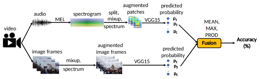
Figure 1: The high-level architecture of the aud-vis baseline proposed for classifying five crowded scenes.

Our dataset of 341 videos were collected from YouTube (in-the-wild scenes), which presents a total recording time of nearly 29.06 hours. These videos are then split into 10-second video segments, each which is annotated by one of five categories of ‘riot’, ‘noise street’, ‘firework event’,‘music event’, or ‘sport atmosphere’. The video segments are split into two subsets of Train and Test with the ratio of 67:33 for the training and inference processes, respectively. Notably, 10-second video segments split from an original video are not presented in both Train and Test subsets to make the data distribution different on these two subsets. The number of 10-second video segments on each subset is shown in Table I.

TABLE I: The number of 10-second video segments corresponding to each scene categories in Train. and Test. subsets

Category	Train	Test	Total
Riot	1429	757	2186
Noise-Street	1430	652	2082
Firework-Event	1406	615	2021
Music-Event	1367	727	2094
Sport-Atmosphere	1365	712	2077
Total	6997	3463	10460
	($\approx$ 19.44 hours)	($\approx$9.62 hours)	($\approx$29.06 hours)

Regarding the evaluation metric, the Accuracy (Acc.%), which is commonly applied in SC challenges such as DCASE Task 1A [1], is used to evaluate the task of crowded scene classification in this paper. Let us consider $M$ as the number of 10-second video segments, which are correctly predicted, from the total number of segments as $N$, the classification accuracy (Acc.%) is computed by

$$Acc.\%=100\frac{M}{N}.$$ (1)

III Proposed Deep Learning Frameworks

III-A The audio, visual, and aud-vis baselines proposed

As we aim to analyse the independent impact of audio or visual input data on the classification task’s performance, proposed deep learning frameworks deploy either audio or visual input data. Then, the results obtained from individual high-performed frameworks are fused to achieve the best performance. To this end, we firstly propose a deep learning framework as described in Figure 1, referred to as the aud-vis baseline. As the Figure 1 shows, the audio and visual input data extracted from a video are deployed by two independent streams, referred to as the audio baseline (e.g. the upper data stream) and the visual baseline (e.g. the lower data stream), before a fusion of predicted probability results of audio and visual streams is conducted.

Regarding the audio baseline as shown in the upper stream in Figure 1, input audio recordings are firstly resampled to 32,000 Hz, then transformed into MEL spectrograms where both temporal and frequency features are presented. By using only one channel and setting parameters of filter number, window size, hop size to 128, 80 ms, 14 ms respectively, we generate MEL spectrograms of $640{\times}128$ from 10-second audio segments. Next, entire spectrograms are split into small patches of $128{\times}128$ that are suitable for back-end classification models. To enforce back-end classifiers, two data augmentation methods of spectrum [8] and mixup [9] are applied on these patches before feeding into a back-end VGGish network for classification. Regarding spectrum augmentation, we apply two zero masking blocks of 10 frequency channels and 10 time frames on each patch of $128{\times}128$. The starting frequency channel or time frame in a masking block is randomly selected. The patches of $128{\times}128$ after spectrum augmentation are then mixed together with different ratios, which is known as the mixup data augmentation. Let’s consider two patches of $128{\times}128$ as $\mathbf{X_{A}}$, $\mathbf{X_{B}}$ and expected labels as $\mathbf{y_{A}}$, $\mathbf{y_{B}}$, we generate new patches as below equations:

$$\mathbf{X_{mx1}}=\gamma\mathbf{X_{A}}+(1-\gamma)\mathbf{X_{B}}$$ (2)

$$\mathbf{X_{mx2}}=(1-\gamma)\mathbf{X_{A}}+\gamma\mathbf{X_{B}}$$ (3)

$$\mathbf{y_{mx1}}=\gamma\mathbf{y_{A}}+(1-\gamma)\mathbf{y_{B}}$$ (4)

$$\mathbf{y_{mx2}}=(1-\gamma)\mathbf{y_{A}}+\gamma\mathbf{y_{B}}$$ (5)

with $\gamma$ is random coefficient from unit distribution or gamma distribution. We feed patches of $128{\times}128$ before and after mixup data augmentation into a back-end VGGish network architecture for classification.

For the visual baseline as shown in the lower stream in Figure 1, two data augmentation methods of spectrum [8] and mixup [9] are also applied on visual data (image frames) before feeding into a back-end VGGish network architecture.

The back-end VGGish networks for audio and visual streams are independent, but share the same architecture as described in Table II. As Table II shows, the VGGish network contains sub-blocks which perform convolution (Conv[kernel size]@channel), batch normalization (BN) [10], rectified linear units (ReLU) [11], average pooling (AP), global average pooling (GAP), dropout (Dr(percentage)) [12], fully connected (FC) and Softmax layers. The dimension of Softmax layer is set to $C=5$ which corresponds to the number of crowded scenes classified. In total, we have 12 convolutional layers and 3 fully connected layers containing trainable parameters that makes the proposed network architecture like VGG15 [13].

TABLE II: The VGG15 network architecture used for both audio and visual baselines.

Network Architecture	Output
BN - Conv [$3{\times}3]$@$32$ - ReLU - BN - Dr (20%)	$128{\times}128{\times}32$
BN - Conv [$3{\times}3]$@$32$ - ReLU - BN - AP - Dr (25%)	$64{\times}64{\times}32$
BN - Conv [$3{\times}3]$@$64$ - ReLU - BN - Dr (25%)	$64{\times}64{\times}64$
BN - Conv [$3{\times}3]$@$64$ - ReLU - BN - AP - Dr (30%)	$32{\times}32{\times}64$
BN - Conv [$3{\times}3]$@$128$ - ReLU - BN - Dr (30%)	$32{\times}32{\times}128$
BN - Conv [$3{\times}3]$@$128$ - ReLU - BN - Dr (30%)	$32{\times}32{\times}128$
BN - Conv [$3{\times}3]$@$128$ - ReLU - BN - Dr (30%)	$32{\times}32{\times}128$
BN - Conv [$3{\times}3]$@$128$ - ReLU - BN - AP - Dr (30%)	$16{\times}16{\times}128$
BN - Conv [$3{\times}3]$@$256$ - ReLU - BN - Dr (35%)	$16{\times}16{\times}256$
BN - Conv [$3{\times}3]$@$256$ - ReLU - BN - Dr (35%)	$16{\times}16{\times}256$
BN - Conv [$3{\times}3]$@$256$ - ReLU - BN - Dr (35%)	$16{\times}16{\times}256$
BN - Conv [$3{\times}3]$@$256$ - ReLU - BN - GAP - Dr (35%)	$256$
FC - ReLU - Dr (40%)	$1024$
FC - ReLU - Dr (40%)	$1024$
FC - Softmax	$C=5$

As back-end classifiers work on patches of $128{\times}128$ or image frames, the predicted probability of an entire spectrogram or all image frames from a 10-second video segment is computed by averaging of all images or patches’ predicted probabilities. Let us consider $\mathbf{P^{n}}=(\mathbf{p_{1}^{n},p_{2}^{n},...,p_{C}^{n}})$, with $C$ being the category number and the $n^{th}$ out of $N$ image frames or patches of $128{\times}128$ fed into a deep learning model, as the probability of a test video, then the average classification probability is denoted as $\mathbf{\bar{p}}=(\bar{p}_{1},\bar{p}_{2},...,\bar{p}_{C})$ where,

$$\bar{p}_{c}=\frac{1}{N}\sum_{n=1}^{N}p_{c}^{n}~{}~{}~{}for~{}~{}1\leq n\leq N$$ (6)

and the predicted label $\hat{y}$ for an entire spectrogram or all image frames is determined as:

$$\hat{y}=argmax(\bar{p}_{1},\bar{p}_{2},...,\bar{p}_{C})$$ (7)

To evaluate the aud-vis baseline, an ensemble of results from the individual audio and visual baselines is conducted. In particular, we proposed three late fusion schemes, namely MEAN, PROD, and MAX fusions. For each scheme, we firstly conduct experiments on the individual audio and visual baselines, then obtain the predicted probability of each baseline as $\mathbf{\bar{p_{s}}}=(\bar{p}_{s1},\bar{p}_{s2},...,\bar{p}_{sC})$ where $C$ is the category number and the $s^{th}$ out of $S$ individual frameworks evaluated. Next, the predicted probability after MEAN fusion $\mathbf{p_{f-mean}}=(\bar{p}_{1},\bar{p}_{2},...,\bar{p}_{C})$ is obtained by:

$$\bar{p_{c}}=\frac{1}{S}\sum_{s=1}^{S}\bar{p}_{sc}~{}~{}~{}for~{}~{}1\leq s\leq S$$ (8)

The PROD strategy $\mathbf{p_{f-prod}}=(\bar{p}_{1},\bar{p}_{2},...,\bar{p}_{C})$ is obtained by:

$$\bar{p_{c}}=\frac{1}{S}\prod_{s=1}^{S}\bar{p}_{sc}~{}~{}~{}for~{}~{}1\leq s\leq S$$ (9)

and the MAX strategy $\mathbf{p_{f-max}}=(\bar{p}_{1},\bar{p}_{2},...,\bar{p}_{C})$ is obtained by:

$$\bar{p_{c}}=max(\bar{p}_{1c},\bar{p}_{2c},...,\bar{p}_{Sc})$$ (10)

Finally, the predicted label $\hat{y}$ is determined by (7).

III-B Further exploring audio-based frameworks

As applying an ensemble of either different types of input spectrograms [14, 15, 16, 17] or different learning models [18, 19, 20, 21, 22] has been a rule of thumb to enhance the performance of audio-based scene classification task performance, we therefore evaluate two ensemble methods, referred to as the multiple spectrogram strategy (e.g. Multiple spectrograms combines with one model) and the multiple model strategy (e.g. Multiple models deploys one type of spectrogram). The multiple spectrogram approach uses three types of spectrograms: Constant Q Transform (CQT) [23], Mel filter (MEL) [23], and Gammatone filter (GAM) [24]. Each spectrogram is then independently classified by one VGG15 as described in Table II. We refer to three frameworks as CQT-VGG15, GAM-VGG15, and MEL-VGG15 (i.e. MEL-VGG15 is known as the audio baseline mentioned in Section III-A), respectively. In the multiple model approach, while only MEL spectrogram is used, different back-end classifiers are evaluated. In particular, we use five benchmarks deep neural network architectures from Keras application library [25]: Xception, Resnet50, InceptionV3, MobileNet, and DenseNet121. We refer to these five frameworks as MEL-Xception, MEL-Resnet50, MEL-InceptionV3, MEL-MobileNet, and MEL-DenseNet121, respectively. In these both approaches, the final classification accuracy is obtained by applying late fusion methods (MAX, MEAN, and PROD) of individual frameworks as mentioned in Section III-A (i.e. An ensemble of three predicted probabilities from CQT-VGG15, GAM-VGG15, and MEL-VGG15, or an ensemble of five predicted probabilities from MEL-Xception, MEL-Resnet50, MEL-InceptionV3, MEL-MobileNet, and MEL-DenseNet121).

III-C Further exploring visual-based frameworks

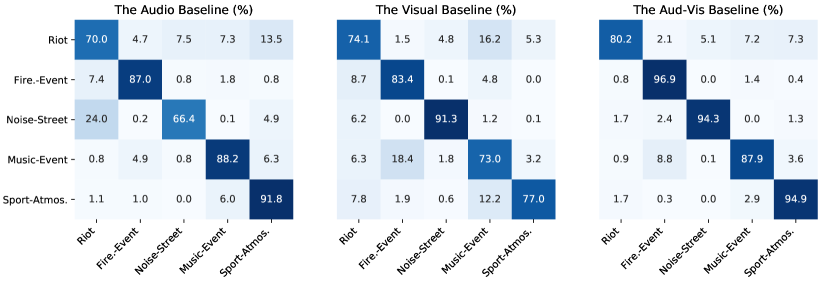
Figure 2: Confusion matrix results of the audio baseline, visual baseline, and aud-vis baseline using PROD fusion.

To further exploring visual-based frameworks, we replace VGG15 by five different network architectures from Keras application library [25]: Xception, Resnet50, InceptionV3, MobileNet, and DenseNet121 which are same and mentioned in Section III-B. Notably, the output nodes at the final fully connected layer of these network architectures is modify from 1000 (e.g. The number of classes in Imagenet dataset) to 5 which matches the number of crowded scene categories. Additionally, we propose two training strategies: Direct Training and Fine-tuning, which are applied on these five network architectures. In Direct Training strategy, all trainable parameters of these five network architectures are initialized with zero and variance set to 0 and 0.1 respectively. Meanwhile in the Fine-tuning strategy, these five networks were trained with ImageNet dataset [26] in advance. We then only reuse the trainable parameters from the first layer to the global pooling layer and train the entire network with a low learning rate of 0.00001. The visual-based frameworks with Direct Training strategy are referred to as visual-direct-VGG15 (i.e. Visual-direct-VGG15 is known as the visual baseline) and visual-direct-Xception, visual-direct-Resnet50, visual-direct-InceptionV3, visual-direct-MobileNet, visual-direct-DenseNet121, respectively. Meanwhile, the visual-based frameworks with Fine-tuning strategy are referred to as visual-finetune-Xception, visual-finetune-Resnet50, visual-finetune-InceptionV3, visual-finetune-MobileNet, and visual-finetune-DenseNet121, respectively. Similar to the audio-based frameworks, the final classification accuracy of the visual-based frameworks is obtained by applying late fusion methods (MAX, MEAN, PROD) of individual frameworks (i.e. An ensemble of predicted probabilities from all frameworks with either Direct Training or Fine-tuning strategies).

III-D Implementation of deep learning frameworks

We use Tensorflow framework to build all classification models in this paper. As we apply spectrum [8] and mixup [9] data augmentation for both audio spectrograms and image frames to enforce back-end classifiers, the labels of the augmented data are no longer one-hot. We therefore train back-end classifiers with Kullback-Leibler (KL) divergence loss [27] rather than the standard cross-entropy loss over all $N$ training samples:

$$LOSS_{KL}(\Theta)=\sum_{n=1}^{N}\mathbf{y}_{n}\log\left(\frac{\mathbf{y}_{n}}{\mathbf{\hat{y}}_{n}}\right)+\frac{\lambda}{2}||\Theta||_{2}^{2},$$ (11)

where $\Theta$ denotes the trainable network parameters and $\lambda$ denotes the $\ell_{2}$-norm regularization coefficient. $\mathbf{y_{c}}$ and $\mathbf{\hat{y}_{c}}$ denote the ground-truth and the network output, respectively. The training is carried out for 100 epochs using Adam method [28] for optimization. All experiments are running on the GeForce RTX 2080 Titan GPUs.

IV Experimental Results and Discussions

IV-A Performance comparison of the audio baseline, visual baseline, and aud-vis baseline

As the confusion matrix results of the audio baseline, the visual baseline, and the aud-vis baseline with PROD fusion are shown in Figure 2, we can see that the audio baseline and the visual baseline are very competitive on ‘Riot’ and ‘Firework-Event’ classes, but they show significant gaps of performance in ‘Noise-Street’, ‘Music-Event’, and ‘Sport-Atmosphere’ categories.

When we apply PROD fusion on predicted probabilities of the audio and visual baselines (e.g. the aud-vis baseline with PROD fusion), performance of all scene categories are significantly improved. This proves that audio or visual input factors have distinct and independent contribution on the task of crowded scene classification proposed.

IV-B Performance comparison of audio-based frameworks

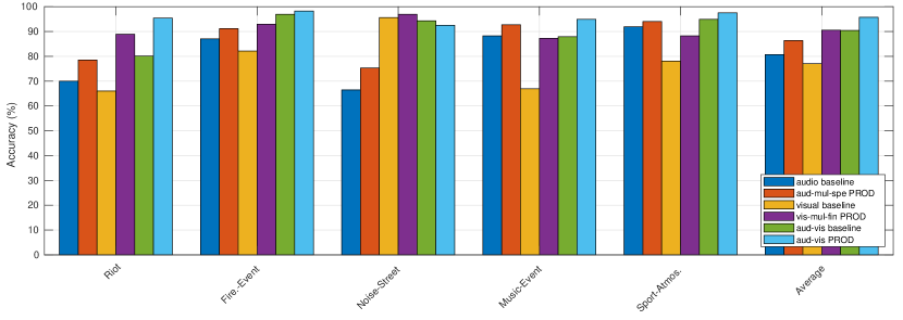
Figure 3: Performance comparison (Acc.%) of audio baseline (MEL-VGG15), aud-mul-spe PROD (PROD fusion of CQT-VGG15, GAM-VGG15, MEL-VGG15), visual baseline (visual-direct-VGG15), vis-mul-fin PROD (PROD fusion of visual-finetune-Xception, visual-finetune-Inception3, and visual-finetune-DenseNet121), aud-vis baseline (PROD fusion of MEL-VGG15 and visual-direct-VGG15), and aud-vis PROD (PROD fusion of CQT-VGG15, GAM-VGG15, MEL-VGG15 and visual-finetune-Xception, visual-finetune-InceptionV3, visual-finetune-DenseNet121) across all scene categories.

As the performance of audio-based frameworks are shown in Table III, we can see that the ensembles of multiple spectrogram or multiple model frameworks help to improve the performance, present the best score of 86.3% and 85.8% from PROD fusion of CQT-VGG15, GAM-VGG15, MEL-VGG15 and MAX fusion of MEL-VGG15, MEL-Xception, MEL-Resnet50, MEL-InceptionV3, MEL-MobileNet, MEL-DenseNet121. These results also indicate that although multiple spectrogram approach uses the low footprint network architecture of VGG15, this approach is more effective than the multiple model approach with high-complexity networks.

Analysing performance on each spectrogram, GAM and MEL achieve competitive results of 83.0% and 80.7% respectively. Meanwhile, CQT shows a slightly poorer performance of 78.6%. However, while a PROD fusion of GAM-VGG15 and MEL-VGG15 achieves 84.2%, PROD fusion of all three spectrograms helps to further improve the performance by 2.1%. This proves that each spectrogram contains distinct features of audio scenes.

For the multiple model approach, it can be seen that individual deep learning frameworks show competitive performance, present the lowest and highest scores of 79.8% and 83.1% from MEL-MobileNet and MEL-DenseNet121, respectively.

IV-C Performance comparison of visual-based frameworks

As the performance of visual-based frameworks is shown in Table IV, we can see that deep learning frameworks with Fine-tuning strategy significantly outperform the same network architectures applying Direct Training strategy. With the Fine-tuning strategy, we can achieve the best accuracy of 88.4% from the single visual-finetune-Xception or visual-finetune-InceptionV3 frameworks. Meanwhile, the best performance of individual frameworks with Direct Training strategy is 80.7% from visual-finetune-Resnet50.

Ensembles of deep learning frameworks regarding both training strategies only help to improve the performances slightly. The results record an improvement of 1.5% and 1.3% for Direct Training and Fine-tuning compared with the best single frameworks of visual-direct-Resnet50 and visual-finetune-Xception, respectively.

IV-D Performance comparison among audio-based, visual-based, and audio-visual frameworks

TABLE III: Performance of audio-based frameworks.

Multiple Spectrogram	Acc.%	Multiple Model	Acc.%
Approach		Approach
MEL-VGG15 (audio baseline)	80.7	MEL-MobileNet	79.8
GAM-VGG15	83.0	MEL-Resnet50	81.4
CQT-VGG15	78.6	MEL-Xception	81.6
		MEL-InceptionV3	81.7
		MEL-DenseNet121	83.1
MAX Fusion	85.5	MAX Fusion	85.8
MEAN Fusion	85.8	MEAN Fusion	85.0
PROD Fusion	86.3	PROD Fusion	85.5

As the comprehensive analysis of independent audio and visual input factors shows in Section IV-B and IV-C, it can be seen that multiple spectrogram approach for audio input data and Fine-tuning strategy for visual input data are effective to enhance the the SC task’s performance. We now combine both visual and audio input factor, then compare: (I) MEL-VGG15 framework known as the audio baseline, (II) PROD fusion of CQT-VGG15, GAM-VGG15, MEL-VGG15 referred to as the aud-mul-spe PROD, (III) visual-direct-VGG15 framework known as the visual baseline, (IV) PROD fusion of visual-finetune-Xception, visual-finetune-InceptionV3 and visual-finetune-DenseNet121 referred to as the vis-mul-fin PROD, (V) PROD fusion of MEL-VGG15 and visual-direct-VGG15 known as the aud-vis baseline, and (VI) PROD fusion of CQT-VGG15, GAM-VGG15, MEL-VGG15 and visual-finetune-Xception, visual-finetune-InceptionV3, visual-finetune-DenseNet121 referred to as the aud-vis PROD (i.e. (VI) is PROD fusion of (II) and (IV)) across all crowded scene categories.

As the results shows in Figure 3, it can be seen that while the audio baseline (MEL-VGG15) and the visual baseline (visual-direct-VGG15) show very competitive average scores of 80.7% and 79.3% respectively, the ensemble of the best three visual based frameworks (vis-mul-fin PROD with 90.5%) outperforms the ensemble of multiple-spectrogram audio based frameworks (aud-mul-spe PROD with 86.3%).

TABLE IV: Performance of visual-based frameworks.

Deep Learning Frameworks	Direct Training	Fine-tuning
	Strategy (Acc.%)	Strategy (Acc.%)
visual-direct-VGG15 (visual baseline)	79.3	-
visual-direct/finetune-MobileNet	78.3	86.9
visual-direct/finetune-Resnet50	80.7	84.8
visual-direct/finetune-Xception	79.4	88.4
visual-direct/finetune-InceptionV3	77.8	88.4
visual-direct/finetune-DenseNet121	79.6	87.0
MAX Fusion	81.6	89.3
MEAN Fusion	82.1	89.5
PROD Fusion	82.2	89.7

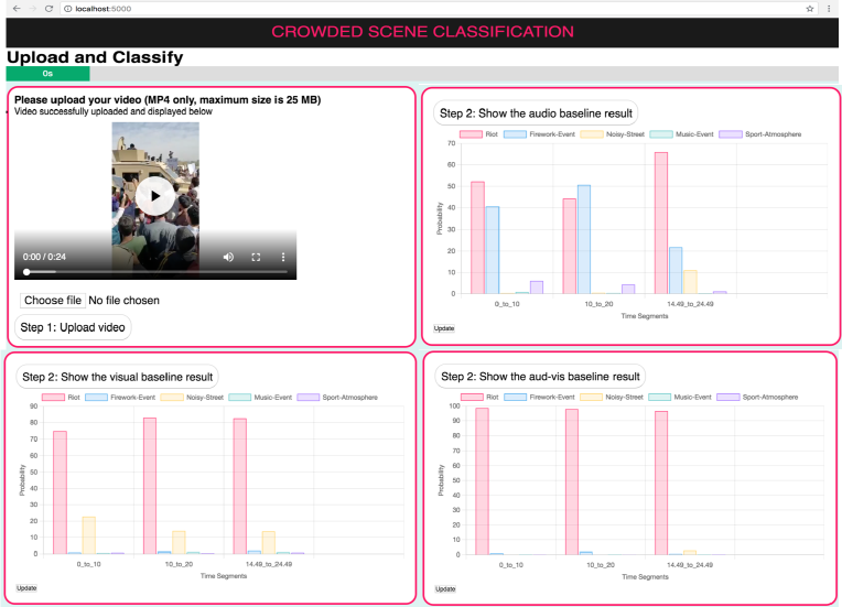
Figure 4: An application demo for audio-visual crowded scene classification.

Compare performance between the aud-vis baseline (e.g. PROD fusion of MEL-VGG15 trained on audio input and visual-direct-VGG15 trained on visual input) and vis-mul-fin PROD (i.e. This approach makes use of Fine-tuning strategy with three large networks of Xception, InceptionV3 and DenseNet121 which are trained with only image input data), it proves that an ensemble of both audio and visual data with the VGG15 architectures is effective to enhance the SC performance significantly (the aud-vis baseline with 90.4%), which is competitive with the fusion of high-complexity network architectures with using only visual data (90.5%). When we conduct PROD fusion of both audio and visual based frameworks (aud-vis PROD), we can achieve the best accuracy of 95.7%.

IV-E An application demo proposed

As we can achieve good results from high-performed deep learning frameworks mentioned in Section IV-D, we then conduct an application demo which uses a HTML front-end interface for uploading an input video and showing classification results on bar charts as shown in Figure 4. The back-end inference process of the demo is the aud-vis baseline with PROD fusion mentioned in Section III-A. As input videos may have different lengths and scene context can be changed by time, bar charts present the classification accuracy on each 10-second segment instead of the entire recording time. By using the Docker software [29], the application of crowded scene classification is packaged to create a docker image for sharing. Given the docker image, the application can be run on a wide range of computers with available docker software setup and easily integrated into any cloud-based system.

V Conclusion

We have proposed an audio-visual dataset of five crowded scenes, then explored different benchmark frameworks on this dataset. Our deep learning framework, which makes use of multiple spectrogram approach for audio input and fine-tuning strategy for visual input, achieves the best performance of 95.7%. The results obtained from our experiments in this paper are very potential to further develop a complex system for detecting relevant-riot context. Our future work is generating an audio-visual-text dataset which comprises both crowded scenes and daily scenes. Given the dataset, we can conduct comprehensive experiments, then propose a powerful indicator to detect a relevant-riot context.

References

- [1] Detection and Classification of Acoustic Scenes and Events Community, DCASE 2021 challenges, http://dcase.community/challenge2021.
- [2] Karol J Piczak, “Esc: Dataset for environmental sound classification,” in Proceedings of the 23rd ACM international conference on Multimedia, 2015, pp. 1015–1018.
- [3] Peng Wu, Jing Liu, Yujia Shi, Yujia Sun, Fangtao Shao, Zhaoyang Wu, and Zhiwei Yang, “Not only look, but also listen: Learning multimodal violence detection under weak supervision,” in European Conference on Computer Vision, 2020, pp. 322–339.
- [4] Waqas Sultani, Chen Chen, and Mubarak Shah, “Real-world anomaly detection in surveillance videos,” in Proceedings of the IEEE conference on computer vision and pattern recognition, 2018, pp. 6479–6488.
- [5] Sercan Sarman and Mustafa Sert, “Audio based violent scene classification using ensemble learning,” in 2018 6th International Symposium on Digital Forensic and Security (ISDFS), 2018, pp. 1–5.
- [6] L. Pham, I. Mcloughlin, Huy Phan, R. Palaniappan, and A. Mertins, “Deep feature embedding and hierarchical classification for audio scene classification,” in International Joint Conference on Neural Networks (IJCNN), 2020, pp. 1–7.
- [7] L. Pham, Huy Phan, T. Nguyen, R. Palaniappan, A. Mertins, and I. Mcloughlin, “Robust acoustic scene classification using a multi-spectrogram encoder-decoder framework,” Digital Signal Processing, vol. 110, pp. 102943, 2021.
- [8] Daniel S Park, William Chan, Yu Zhang, Chung-Cheng Chiu, Barret Zoph, Ekin D Cubuk, and Quoc V Le, “Specaugment: A simple data augmentation method for automatic speech recognition,” arXiv preprint arXiv:1904.08779, 2019.
- [9] Yuji Tokozume, Yoshitaka Ushiku, and Tatsuya Harada, “Learning from between-class examples for deep sound recognition,” in International Conference on Learning Representations (ICLR), 2018.
- [10] Sergey Ioffe and Christian Szegedy, “Batch normalization: Accelerating deep network training by reducing internal covariate shift,” in Proceedings of the 32nd International Conference on Machine Learning, 2015, pp. 448–456.
- [11] Vinod Nair and Geoffrey E Hinton, “Rectified linear units improve restricted boltzmann machines,” in International Conference on Machine Learning (ICML), 2010.
- [12] Nitish Srivastava, Geoffrey Hinton, Alex Krizhevsky, Ilya Sutskever, and Ruslan Salakhutdinov, “Dropout: a simple way to prevent neural networks from overfitting,” The Journal of Machine Learning Research, vol. 15, no. 1, pp. 1929–1958, 2014.
- [13] Karen Simonyan and Andrew Zisserman, “Very deep convolutional networks for large-scale image recognition,” in International Conference on Learning Representations (ICLR), 2015.
- [14] L. Pham, I. McLoughlin, H. Phan, R. Palaniappan, and Y. Lang, “Bag-of-features models based on C-DNN network for acoustic scene classification,” in Proc. International Conference on Audio Forensics (AES), 2019.
- [15] Lam Pham, Ian Mcloughlin, Huy Phan, and Ramaswamy Palaniappan, “A robust framework for acoustic scene classification,” in Proc. International Speech Communication Association (INTERSPEECH), 2019, pp. 3634–3638.
- [16] D. Ngo, Hao Hoang, A. Nguyen, Tien Ly, and L. Pham, “Sound context classification basing on join learning model and multi-spectrogram features,” ArXiv, vol. abs/2005.12779, 2020.
- [17] Lam Pham, Hieu Tang, Anahid Jalali, Alexander Schindler, and Ross King, “A low-compexity deep learning framework for acoustic scene classification,” arXiv preprint arXiv:2106.06838, 2021.
- [18] Hyeji Seo, Jihwan Park, and Yongjin Park, “Acoustic scene classification using various pre-processed features and convolutional neural networks,” in Proceedings of the Detection and Classification of Acoustic Scenes and Events Workshop (DCASE), New York, NY, USA, 2019, pp. 25–26.
- [19] Jonathan Huang, Hong Lu, Paulo Lopez Meyer, Hector Cordourier, and Juan Del Hoyo Ontiveros, “Acoustic scene classification using deep learning-based ensemble averaging,” .
- [20] Yang Haocong, Shi Chuang, and Li Huiyong, “Acoustic scene classification using cnn ensembles and primary ambient extraction,” Tech. Rep., 2019.
- [21] Truc Nguyen and Franz Pernkopf, “Acoustic scene classification using a convolutional neural network ensemble and nearest neighbor filters,” in Proc. DCASE, 2018, pp. 34–38.
- [22] Huy Phan, Huy Le Nguyen, Oliver Y. Chén, Lam Pham, Philipp Koch, Ian McLoughlin, and Alfred Mertins, “Multi-view audio and music classification,” in Proc. IEEE International Conference on Acoustics, Speech and Signal Processing (ICASSP), 2021, pp. 611–615.
- [23] Brian McFee, Raffel Colin, Liang Dawen, D.P.W. Ellis, McVicar Matt, Battenberg Eric, and Nieto Oriol, “librosa: Audio and music signal analysis in python,” in Proceedings of The 14th Python in Science Conference, 2015, pp. 18–25.
- [24] D. P. W. Ellis, “Gammatone-like spectrogram,” 2009.
- [25] François Chollet et al., “Keras,” https://keras.io, 2015.
- [26] Olga Russakovsky, Jia Deng, Hao Su, Jonathan Krause, Sanjeev Satheesh, Sean Ma, Zhiheng Huang, Andrej Karpathy, Aditya Khosla, Michael Bernstein, Alexander C. Berg, and Li Fei-Fei, “ImageNet Large Scale Visual Recognition Challenge,” International Journal of Computer Vision (IJCV), vol. 115, no. 3, pp. 211–252, 2015.
- [27] Solomon Kullback and Richard A Leibler, “On information and sufficiency,” The annals of mathematical statistics, vol. 22, no. 1, pp. 79–86, 1951.
- [28] Diederik P. Kingma and Jimmy Ba, “Adam: A method for stochastic optimization,” CoRR, vol. abs/1412.6980, 2015.
- [29] Dirk Merkel, “Docker: lightweight linux containers for consistent development and deployment,” Linux journal, vol. 2014, no. 239, pp. 2, 2014.