Observations with the Southern Connecticut Stellar Interferometer. I. Instrument Description and First Results

Abstract

We discuss the design, construction, and operation of a new intensity interferometer, based on the campus of Southern Connecticut State University in New Haven, Connecticut. While this paper will focus on observations taken with an original two-telescope configuration, the current instrumentation consists of three portable 0.6-m Dobsonian telescopes with single-photon avalanche diode (SPAD) detectors located at the Newtonian focus of each telescope. Photons detected at each station are time-stamped and read out with timing correlators that can give cross-correlations in timing to a precision of 48 ps. We detail our observations to date with the system, which has now been successfully used at our university in 16 nights of observing. Components of the instrument were also deployed on one occasion at Lowell Observatory, where the Perkins and Hall telescopes were made to function as an intensity interferometer. We characterize the performance of the instrument in detail. In total, the observations indicate the detection of a correlation peak at the level of 6.76$\sigma$ when observing unresolved stars, and consistency with partial or no detection when observing at a baseline sufficient to resolve the star. Using these measurements we conclude that the angular diameter of Arcturus is larger than 15 mas, and that of Vega is between 0.8 and 17 mas. While the uncertainties are large at this point, both results are consistent with measures from amplitude-based long baseline optical interferometers.

1 Introduction

Intensity interferometry, first proposed by Hanbury Brown & Twiss (1956, 1958), can be used as a method of extracting very high resolution information of astrophysical sources based on the super-Gaussian statistics of photons, also referred to as the Hanbury Brown and Twiss (HBT) effect. They showed that light recorded by two independent detectors at different locations has a weak correlation in intensity if the object being viewed was indistinguishable from a point source. In astronomical terms, this implies that if the two detectors are separated by a distance less than that needed to resolve a star, then the intensity correlation should be observed. In contrast, when the distance is increased to the point where the baseline resolves the object, the correlation disappears. In between these two limits, partial correlation can be observed that traces out the profile of an Airy pattern, the width of which is inversely proportional to the diameter of the star being observed. Hanbury Brown and his collaborators were able to measure the diameters of 32 stars from the site of their famous Narrabri intensity interferometer (Hanbury Brown, Davis & Allen, 1974), which represented the culmination of their intensity interferometry efforts. Chronologically, this work sat between the seminal interferometric studies of Michelson and Pease performed at the Mount Wilson 2.5-m telescope (Michelson & Pease, 1921; Pease, 1925) and the development and use of the Mark III stellar interferometer in the 1980’s and 1990’s (Shao et al., 1988; Hutter et al., 1989; Hummel et al., 1995). The latter paved the way for the return to amplitude-based optical interferometry and the rise of specialized facilities for long baseline optical interferometry such as SUSI (Davis, 1994; Tango, 2003; Davis et al., 2005), the Navy Precision Optical Interferometer (Armstrong et al., 1998; Nordgren et al., 1999; Baines et al., 2018), the CHARA Array (McAlister et al., 2005; ten Brummelaar et al., 2005; Schaefer et al., 2020), and the Magdalena Ridge Optical Interferometer (Creech-Eakman et al., 2004, 2018, 2020).

Starting in the mid-2000’s, however, a revival of intensity interferometry has slowly taken shape. One of the principal reasons for this is that ultra-fast detectors with high quantum efficiencies have become widely available. This allows for a re-examination of the technique in a photon-counting context with the advantage that increased speed creates the possibility of higher signal-to-noise ratios (SNRs) as detailed in Klein, Guelman, & Lipson (2007). Those authors discuss the fact that the timing capabilities of modern detectors and timing correlators can be as much as a factor of 1000 higher than those of the instrumentation used at Narrabri, which gives flexibility in the design of a modern intensity interferometer. For example, whereas the Narrabri instrument used two telescopes with primary mirror diameters of 6.5 m to achieve a limiting magnitude of approximately $V$=2, the higher timing resolution of modern detectors allows one to achieve the same limiting magnitude with telescopes that are much smaller. Alternatively, significantly fainter limiting magnitudes are now possible with telescopes that are comparable in size to the Narrabri instrument. Several groups have built new intensity interferometers and reported successful correlation measurements in recent years, including Rivet et al. (2018, 2020); Acciari et al. (2020); Abeysekara et al. (2020); and Zampieri et al. (2021). The intrinsic timing resolution of these instruments spans a range from roughly 400 ps to 2.5 ns and they use telescopes with diameters of 1 to 17 m; in the case of larger telescopes (Acciari et al., 2020; Abeysekara et al., 2020), these are so-called “light-bucket” telescopes, which do not have high optical resolution, and as a consequence, detectors with a larger active area must be used to collect the light, generally photomultiplier tubes. Thus these instruments are much closer in design to the Narrabri stellar interferometer of the 1970s. In contrast, the employment of smaller ($\sim$1-m class) telescopes (Rivet et al., 2018; Zampieri et al., 2021) has generally been coupled with the use of ultra-fast single-photon avalanche diode (SPAD) detectors.

Over the last several years, our group has designed, built, and operated a new intensity interferometer based mainly at the campus of Southern Connecticut State University, but which is modular enough to transport the photon-detection instrumentation to other astronomical facilities (Horch & Camarata, 2012; Horch et al., 2016, 2018; Weiss, Rupert, & Horch, 2018; Klaucke et al., 2020). It belongs to the second category of intensity interferometers just mentioned in that it uses 0.6-m telescopes and SPAD detectors. We describe in this paper the final instrument design and construction, discuss the observations taken to date both on our campus and at the Anderson Mesa site at Lowell Observatory, and analyze the results obtained with the data so far. While we are still improving the instrument performance and the data-taking process, these observations together indicate that the system is detecting intensity correlations at the level predicted by theory. Our instrument uses smaller telescopes than any of the other intensity interferometers mentioned above and its timing precision is higher, thus it pushes the technique into a regime where it can be done with portable telescopes and at relatively low cost. We use the correlations detected to make deductions concerning the diameters of Vega ($\alpha$ Lyr, HR 7001), and Arcturus ($\alpha$ Boo, HR 5340); while still uncertain, these measurements are consistent with those made with the larger Michelson-style optical interferometers.

2 Basic Theory

The details of optical detection depend on the properties of photons, which follow Bose-Einstein statistics. As discussed in e.g. Mandel (1963) and Hanbury Brown (1974), if $n$ photons are detected on average in a time interval $\Delta t$, then the variance in the detection rate for a linearly polarized input beam is given by

$$(\Delta n)^{2}=n+n^{2}\frac{\Delta\tau}{\Delta t},$$ (1)

where $\Delta\tau$ represents the coherence timescale over which intensity variations occur due to Bose-Einstein fluctuations and is related to the inverse of the frequency bandwidth of the detected light. The presence of the second term on the right-hand side of the equation indicates that over time intervals of order $\Delta\tau$ or less there will be an increased probability of photon detection, which represents the HBT effect and is sometimes referred to as photon bunching. In most applications, however, $\Delta\tau$ is at least several orders of magnitude smaller than $\Delta t$ and the deviation from Poisson statistics is negligible.

The possibility for using this effect in high-resolution imaging in astronomy arises from the fact that the second order coherence function, which depends on the expression for the variance above, is also related to the modulus square of the complex visibility. The former is defined as

$$g^{(2)}({\bf r},{\bf b},t,t_{0})=\frac{\left<I_{1}({\bf r},t)\cdot I_{2}({\bf r}+{\bf b},t+t_{0})\right>}{\left<I_{1}({\bf r},t)\right>\cdot\left<I_{2}({\bf r},t)\right>},$$ (2)

where the brackets indicate a time average, $I_{1}$ and $I_{2}$ are the irradiance values at two different detection points, ${\bf r}$ is a fixed detection point in space, ${\bf b}$ is the baseline between ${\bf r}$ and a second detection location, and $t_{0}$ is the timing delay between detection at the two stations. Defining the complex visibility as $V_{12}$, the relationship between $g^{(2)}$ and $V_{12}$ in the case of linearly polarized light can be written as

$$g^{(2)}_{\rm pol}=1+|V_{12}|^{2}\frac{\Delta\tau}{\Delta t}.$$ (3)

For the case of unpolarized light, Mandel (1963) shows that, because the second order coherence function involves the products of intensities and not field amplitudes, the expected result for $g^{(2)}$ for unpolarized light modifies the last term in the above by a factor of 1/2:

$$g^{(2)}_{\rm unpol}=1+\frac{1}{2}|V_{12}|^{2}\frac{\Delta\tau}{\Delta t}.$$ (4)

Regardless of the polarization state of the detected light, Equations 3 and 4 establish the fact that high-resolution information about a source can be obtained by detecting the irradiance at two locations without physically interfering the light. For a photon-counting experiment, Equation 2 indicates that the data product needed to obtain $g^{(2)}$ (and therefore $|V_{12}|^{2}$) is the normalized timing cross-correlation of the photon data streams. However, in order to retrieve high-quality data and determine the visibility, it is crucial to increase the fraction $\Delta\tau/\Delta t$ as much as possible. This can be done by decreasing the frequency bandwidth of the light by using an extremely narrow-bandpass filter (which increases the numerator), or by increasing the electronic bandwidth of the detector (which decreases the denominator), or both. Much of the recent revival of intensity interferometry has been made possible by detector developments that have enabled the second of these options.

To estimate the signal-to-noise ratio (SNR) that is practically obtainable in the unpolarized case, we follow Malvimat, Wucknitz & Saha (2014). In a given timing interval $\Delta t$, there will be approximately $\Delta t/\Delta\tau$ intervals of coherence. If the count rate per second is given by $r$, then the number of counts detected per interval at each telescope is given by $n=r\Delta t$. The total number of photon correlations generated per timing interval is the square of this, $(r\Delta t)^{2}$, and each of these has a probability of $\Delta\tau/\Delta t$ of being correlated due to the HBT effect (with the remainder being “random” correlations), yielding a signal of

$$S=\frac{1}{2}(r\Delta t)^{2}\cdot\frac{\Delta\tau}{\Delta t}=\frac{r^{2}\Delta\tau\Delta t.}{2}$$ (5)

On the other hand, the noise would be dominated by Poisson statistics even at the detector speeds available today, and given by the square root of the number of random correlations obtained per interval, or in other words,

$$N=r\Delta t.$$ (6)

Therefore, the SNR is given by

$${\rm SNR}(\Delta t)=\frac{r\Delta\tau}{2}.$$ (7)

Over a longer integration time, the result from each counting interval would add in quadrature, so that in a total exposure time of $T$, the final SNR would be given by

$${\rm SNR}(T)=\frac{r\Delta\tau}{2}\sqrt{\frac{T}{\Delta t}}.$$ (8)

All of the quantities on the right-hand side of this equation are direct observables except the coherence time $\Delta\tau$. However, this is easily obtained from characteristics of the filter used to make the observations. We calculate the frequency bandwidth from filter properties as

$$\Delta\nu=\frac{c}{\lambda_{0}-\Delta\lambda/2}-\frac{c}{\lambda_{0}+\Delta\lambda/2},$$ (9)

where $\lambda_{0}$ is the center wavelength of the observation and $\Delta\lambda$ is the full width at half maximum (FWHM) of the filter transmission. While the coherence time depends to a certain extent on the shape of the filter transmission curve, it can be approximated as

$$\Delta\tau\approx\frac{1}{\Delta\nu}.$$ (10)

Once $\Delta\tau$ is calculated for a given filter, the fraction of photons correlated due to the HBT effect is $\Delta\tau/(2\Delta t)$ in the unpolarized case. For example, with a filter width of 3 nm and center wavelength of 532 nm, $\Delta\tau\approx 0.31$ ps; using a timing resolution of 64 ps to record the data, the expected fraction of correlated photons is then 0.0024. At a constant count rate of 1 MHz at each telescope (which, as we will show in Section 4, we can generally obtain on the 2nd magnitude star Polaris [$\alpha$ UMi]), a 5-$\sigma$ correlation peak above the noise (SNR = 5) would be obtained when $T\approx 19$ hours of observing an unresolved star ($|V_{12}|^{2}=1$). Using a narrower filter would result in a larger fraction of correlated photons but fewer photons detected in the same proportion, so the SNR for a given observing time $T$ remains the same.

3 Instrument Description

The instrument we have constructed and used to date is a two-station interferometer where, for on-campus observing, the two telescopes may be easily moved to observe at a desired baseline and orientation. The telescopes used are 0.6-m Dobsonian telescopes made by Equatorial Platforms of Grass Valley, California. Each has a focal length of 2 m, so that the plate scale at the Newtonian focus is approximately 0.1 arcsec per micron. We have recently obtained a third identical telescope, and future observations with the instrument will be made with all three stations deployed.

An image of the main components and a block diagram of the interferometer are shown in Figure 1. We place a single photon avalanche diode (SPAD) detector at the Newtonian focus of each telescope. Until 2019, we used two Micro Photon Devices (MPD) PDM series SPADs with a 50 micron-diameter active area; given the plate scale mentioned above, this maps to a 5-arcsecond diameter region on the sky. Starting in 2019, we began using two 100-micron diameter PDM-series SPADs. We also have a $1\times 8$ SPAD array from the Politecnico di Milano, Italy. A detailed description of the array is given in Cammi et al. (2012); however, this device was only used on one occasion for the observations described below. Generally, the timing uncertainty of cross-correlations made with any of these detectors is about 50 ps, and the dead time is about $\sim$80 ns after each detected photon. This limits the count rate that can be detected to less than about 10 MHz, but for astronomical purposes, this is not a significant limitation since the expected count rate will be below this limit for most stars we wish to observe.

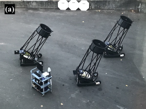
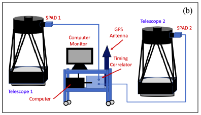
Figure 1: (a) The instrument set up at the standard observing location on the SCSU campus. (b) A block diagram of the simpler two-telescope arrangement, which will be the focus of this paper.

To mount the detector on the telescope, it is placed in a harness made from a tube of PVC pipe. The tube is cut so that it is in contact with the body of the detector and holds it from the top and bottom. The arrangement is held in place with elastic bands that create a pressure fit onto the back of the tube. Inside the tube is an optical assembly consisting of a 35-mm focal length acromat lens, followed by a narrow band pass filter, followed by a second lens that is identical to the first. With the front lens at the correct position in the focus tube of the telescope, a collimated beam is created between the lenses, as the light passes through the filter. Once reimaged by the second lens, the light is focused on the detector with no change in plate scale relative to the Newtonian focus. We currently have three filters available for use with the set up that have specifications shown in Table 1. No polarizers are used in the optical system.

Two timing correlators have been used with the instrument so far to read out and record the events detected by the SPAD detectors: a PicoHarp 300 and a HydraHarp 400, both made by PicoQuant, Inc. The former has two input channels, whereas the latter has eight. Both devices have a time-tagging mode, where each photon event that is detected in any channel is time-stamped, and the timing address and channel number are written out in a 4-byte block. In this mode, the least significant bit of the address corresponds to 4 ps in the case of the PicoHarp and 1 ps in the case of the HydraHarp. For the PicoHarp, the timing addresses are the lower 28 bits of this address and the upper four bits encode the channel number, so that in a typical observation for a single data file of 10s or 100s of seconds, the timing address will roll over many times, roughly once per 0.8 ms. Each time the counter rolls over, an event is written with a special code in the top 4 bits to indicate that a rollover has occurred rather than a photon event. By keeping track of the total number of roll-overs that have occurred as the events are subsequently processed, a unique timing can be associated to each event even in a long observation. For the HydraHarp, the upper six bits of the four byte data word are reserved for encoding the channel number corresponding to the event and special event markers; in this case, because the number of timing bits is lower and yet the timing resolution is higher, rollovers in timing occur roughly once per 30 microseconds. To minimize the number of rollover markers written when count rates are low, the rollover data word also contains the number of rollovers since the last photon event.

Events are read out with a small desktop computer that is placed on a table or a cart near the observing site. An observation file is stored with a header that contains basic instrument parameters, followed by the sequence of time stamps for recorded events. A typical 5-minute file where the count rate on each channel is 1 MHz results in a file that is approximately 2.5 GB in size; a typical observing session of 4 hours can therefore yield over 100 GB of data.

Table 1: Current SCSI Filter Options

Manufacturer	$\lambda_{0}$	$\Delta\lambda$	Max.
	(nm)	(FWHM, nm)	Trans.
Edmund Optics	532	2.02 – 3.7	0.90
Edmund Optics	532	1.2	0.95
Newport Optics	633	1.0	0.30

4 Expected System Performance

While optical path length requirements in intensity interferometry are not as stringent as in amplitude-base interferometry, our instrument relies on photon counting with extremely high timing resolution. Given this, coincidence of photon arrivals can be affected at a level important for our data reduction in three main ways: (1) electronic delay based on detector response, propagation of the signals through cable, and intrinsic timing differences between readout channels in the timing correlators, (2) optical delay within each telescope system, and (3) geometrical delays based on the location of the star on the sky at the time of observation. We discuss each aspect of the performance that we can expect from our instrument below.

4.1 Electronic Considerations

Detector response is the primary factor that will influence the detected correlation. Our detectors have measured FWHM timing uncertainties of approximately 30 ps. This means that two photons that are correlated are not generally detected as coincident in time, but could differ by tens of ps in terms of when the first detector pulse is created versus the second. The correlation signal, which is a delta function in the perfect case, is therefore smeared out in time. The timing correlator then time-stamps the pulses as they arrive, and when the cross-correlation function is computed from the events collected, the delta function is approximately recovered if the timing interval $\Delta t$ is chosen to match the width of the smeared peak. In our case, because each detector has a FWHM of 30 ps, the cross-correlation width should be approximately $30\cdot\sqrt{2}=$ 42 ps in width, just from the detector timing characteristics.

Two further contributions to this smearing arise from the spreading of the pulse as it travels through the cable to the timing module and from the intrinsic timing resolution of the timing correlator itself (regardless of the precision of the timing address). To measure these effects, we split the output cable from a single detector into two lines, and fed these into two (independent) channels of the timing correlator in the laboratory. We then exposed the detector assembly (the SPAD detector and the fore-optics) to diffuse light, and read out pulses from both channels. In this case, the uncertainty in the detector timing is eliminated because we correlate the same pulses, just repeated in the two channels. In cross-correlating events from a data file taken in this way, we find a FWHM of approximately 24 ps for the typical cable lengths that we use for on-campus observing. On this basis, we conclude that the final intrinsic limitation of the timing resolution of a cross-correlation between channels is approximately $\sqrt{42^{2}+24^{2}}=48$ ps for our system.

Using the same experimental set-up, we can also measure any intrinsic timing offset between the read-out channels as well as the timing delay associated with each cable. Figure 2(a) shows sample results that we obtain when inserting three short extra cable lengths into one of the two channels prior to taking data. Repeated measurements indicate that cable delays are determined with a precision of approximately 6 ps. We also find that small intrinsic offsets do exist between the channels of our correlators, on the order of a few tens of ps for the two channels in the PicoHarp, and as much as $\sim$400 ps for channels in the HydraHarp. Furthermore, these offsets appear to drift over a period of months by 10-20 ps. To account for this, we measured the offsets and cable delays about 3-4 times per year, and apply the offsets obtained closest in time to the observations being reduced.

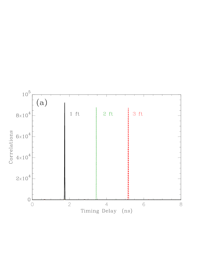
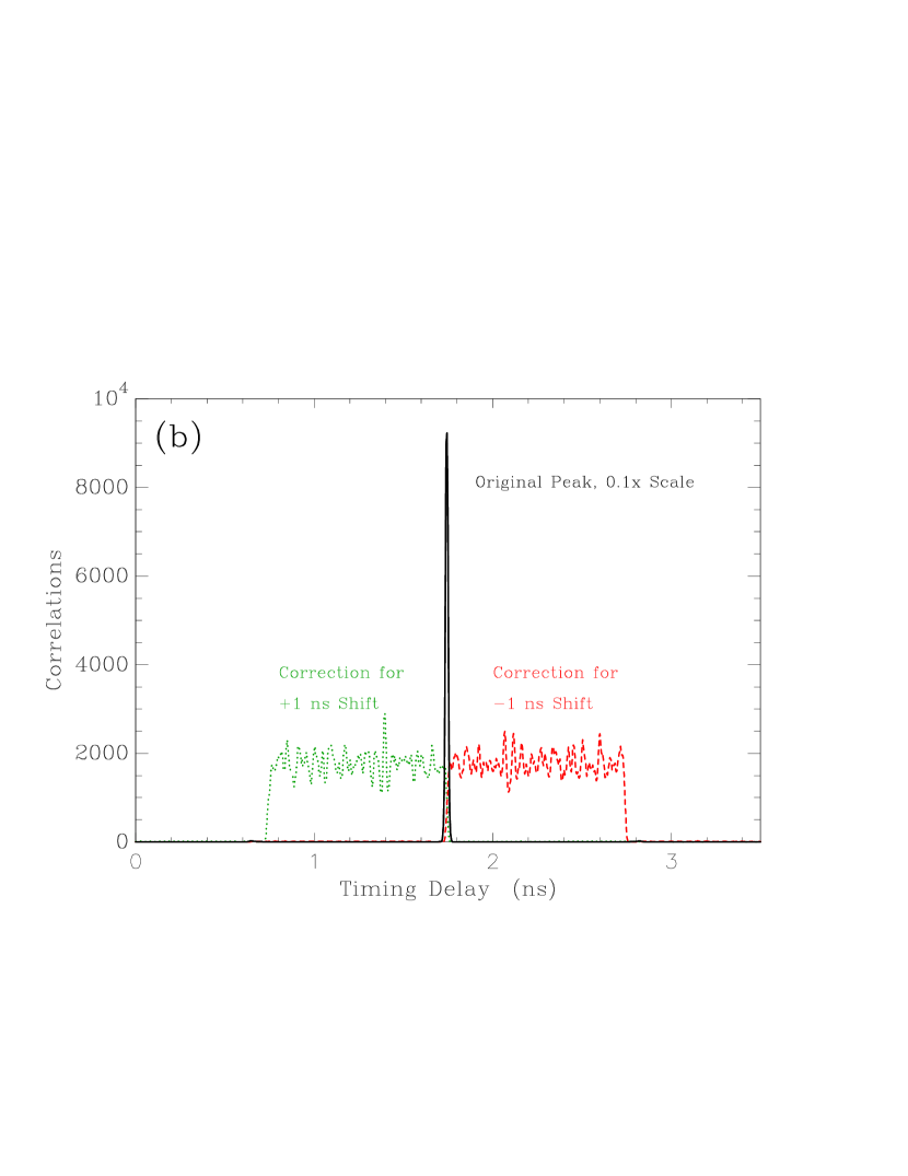
Figure 2: (a) Correlation plots for three different cable inserts placed into one channel. The signal from a single detector is split as described in the text and then cable inserts of 1, 2, and 3 feet are added to the Channel 1 cable run. (b) A test of the timing correction software by using a data file as in (a). There is no delay through the file, but if we attempt a correction for a shift of the peak in either direction, the correlations are spread out in the opposite direction, as expected.

We also used this experimental set-up to check that our software computing the cross-correlation function is working properly. For reducing data from stars, the changing position of the object across the sky implies that the delay between the two channels also changes. Thus, one must correct for this effect in software, even within a single data file containing a few minutes of data. The lab measurements of course do not have this effect, so that if we analyze the lab data as if the peak position is changing, we should observe a smearing of the correlation peak in the opposite direction. In Figure 2(b), we show the result when assuming the file has a $\pm$1 ns shift in the location of the peak during the exposure time. (A typical expected shift for our observing sessions would be on the order of 1 to a few ns, depending on baseline, sky position, and the time spent on the target.) The (strongly-peaked) original cross-correlation function is then spread into a top-hat function in the expected direction and with the correct width.

Lastly, when the time stamps for photons in each channel are to be cross-correlated, a coincidence requirement must be established. In general, one would expect that the timing “bins” would be chosen so that they have nearly the same width as the expected cross-correlation response discussed just above of 48 ps. However, to verify this, we constructed a simulation program that outputs data with effective time stamps as short as 1 ps, but with the combination of detector timing and electronic jitter at the measured level. To do this, the cross-correlation function is constructed directly with 1-ps timing bins as follows. We select a mean number of random correlations per bin and a fraction of correlated photons for the simulation. The parent probability function for the cross-correlation is then a constant function with value of the mean number of correlations per picosecond plus a Gaussian function with integral determined by the fraction of correlated photons and with width given by the detector plus electronic jitter as discussed above. We then select Poisson deviates from the input values in each 1-ps timing bin in the parent distribution. By rebinning the 1-ps precision cross-correlation to different, coarser bin widths, we can investigate the effect on the SNR. This simulates using different timing bin widths (coincidence requirements) in the analysis. The results are shown in Figure 3, where in the left panel, the SNR obtained as a function of timing bin width is shown for four different simulations. In the right panel, we compare the level of SNR observed as a fraction of the theoretical value input into the simulation. At the peak value, the SNR calculated from the data is 89% of the theoretical value, at a bin width of 64 ps. (It is not 100% of the value one would calculate from Equation 8 because timing jitter sends some correlated photons into the wings of the detector response and thus they did not appear in the timing bin of the expected peak location.) If a timing bin above 64 ps is used to establish coincidence, then more signal counts are included, but at the price of a higher number of random correlations. On the other hand, if a bin width less than 64 ps is used, more signal counts fall outside the criterion for coincidence, also leading to a loss of SNR. For the data described in this paper, a timing bin of 64 ps will be used in the data reduction for all observations here.

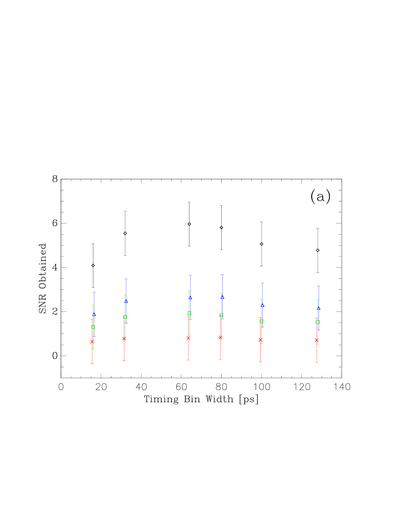
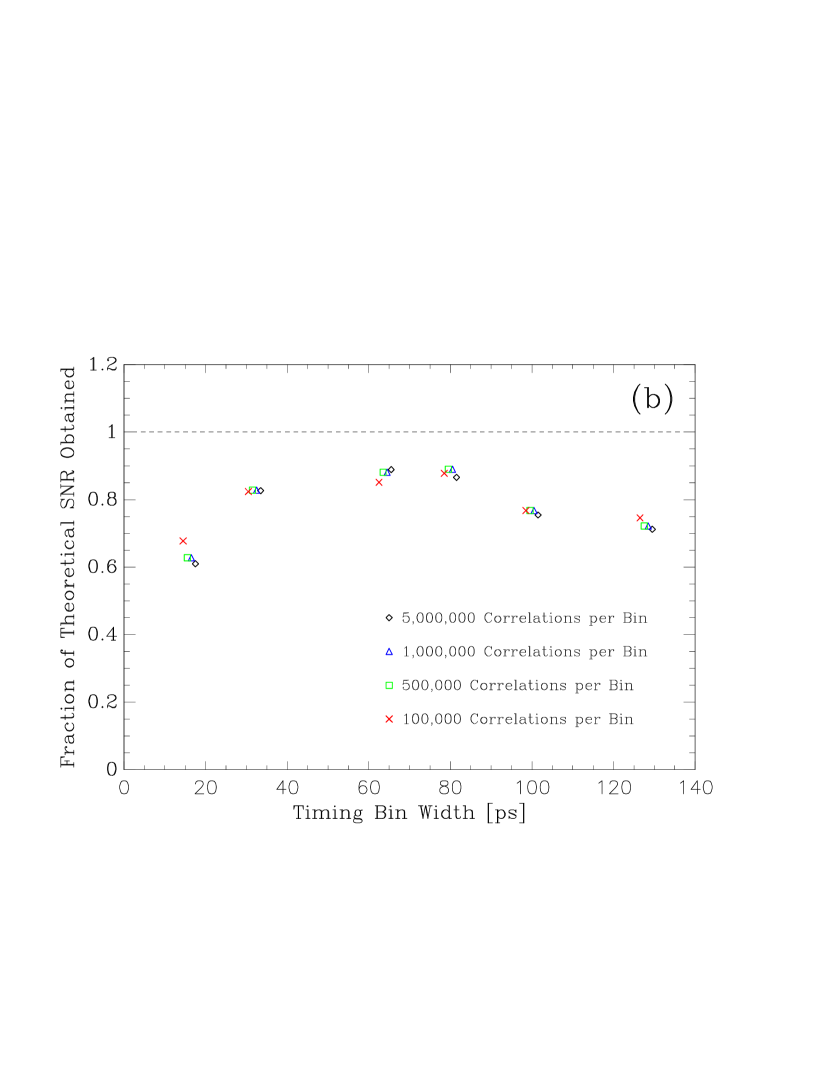
Figure 3: (a) Signal-to-noise ratio (SNR) obtained in simulation results assuming a timing uncertainty of 30 ps for each detector and 20 ps uncertainty in the time stamp from the correlator. These are shown as a function of the timing bin width used to correlate the data, and span a wide range of count rates and total exposure times per night. (b) The same data shown as a fraction of the theoretical SNR. Here the error bars are removed for clarity. In both plots, some of the symbols are offset slightly in the horizontal direction to avoid overlap.

4.2 Optical Considerations

Another factor that can reduce the degree of correlations seen is a red leak or other out-of-band contributions to the light that reaches the detector through the optical system. By using standard incandescent, fluorescent, and LED light sources in the laboratory, we have checked for any evidence of measurable out-of-band light reaching the detectors through the optical harness that includes the filter. Reflecting the light off of a white, flat screen and covering the detector assembly in black cloth except for the entrance pupil, we detect counts through the optical harness, i.e. the detector assembly as it is attached to the telescope. For the 633-nm and narrow 532-nm filters, count rates obtained in the lab do not show evidence for measurable out-of-band contributions; the ratio of counts obtained is, after accounting for the difference in spectral power generated by each lamp at the two different wavelengths, largely consistent with the known widths and peak transmissions of the filters. On the other hand, the wider 532-nm filter has a larger-than-expected count rate when viewing the incandescent source, suggesting that this filter has a red leak. This implies that some percentage of the light we detect from stars in this filter will be uncorrelated, even when viewing an unresolved object, decreasing the correlated fraction of light by the same percentage as the out-of-band light to the total amount detected. By using standard (blackbody) emission curves available for an incandescent source we find we are able to approximately match the observed count rate obtained by including a red leak transmission model of perhaps ten percent transmission in the range of 750-1100 nm.

The stellar sources we observe have spectra that peak at much bluer wavelengths than the standard incandescent laboratory light source. If one assumes a red leak at this level and computes the out-of-band fraction of light that would be obtained for the spectral type of each star we have observed, we find that the out-of-band contribution is at most a few percent. The spectra found in the spectral library of Pickles (1998) were used for this calculation. As a consequence, we will ignore this effect at present. Nonetheless, the wider 532-nm filter is likely to be useful to us, particularly on the fainter sources we wish to observe, so we plan to more fully characterize the transmission at all wavelengths in the future.

An effect that the optical design may have on the width of the correlation peak is to create a spread due to optical path length differences between paraxial and marginal rays in the optical system. However, to first order the telescopes themselves will not contribute to this because the figures of their mirrors are such that they give good image quality at the Newtonian focus. A marginal ray will reflect off of the primary mirror first for a plane wave input beam, but it travels a longer distance to reach the focal point, largely canceling the initial timing difference from the point of reflection. The optical harness in front of the detector includes two lenses, and one may roughly estimate the maximum possible optical path difference from the telescope focus to the detector focus using a thin lens approximation. A paraxial ray would travel up to the first lens along the optical axis while a marginal ray will travel the hypotenuse of the triangle whose legs are the focal length of the lens (35 mm) and the radius of the lens (12.5 mm), a difference in distance of 2.2 mm. Because the second lens reimages the light onto the detector with the same focal length, the optical path difference estimate is simply the double of this, namely $\sim$4.4 mm. In time, this difference amounts to a maximum delay of 14 ps in terms of the arrival time of the photons. Averaging over all rays uniformly distributed in the collimated beam of a circular aperture, the result would be 7.5 ps with a standard deviation of 4.3 ps. Thus, we will ignore this spread in the work presented later in this paper.

4.3 Geometrical Timing Delay and Telescope Placement

We define the geometrical timing delay as the timing difference between when a photon would reach the input pupil on Telescope 1 versus when it would reach Telescope 2. This delay is therefore equivalent to the path length difference between the two telescopes starting from the same wavefront above the telescope apertures, divided by the speed of light. If the star being observed is overhead or on the Great Circle that passes through the zenith and is perpendicular to the orientation of the baseline, then this timing delay would be zero, but depending on the position of the object on the sky, there can be a substantial difference in arrival times between correlated photons, especially given our level of timing precision. The consequence of this is that, during data taking, the position of the correlation peak in the cross-correlation will shift as the star’s diurnal motion across the sky proceeds. As discussed by Dyck (1999), the timing delay, $\Delta$, may be calculated as

$$\Delta=-\frac{b_{E}}{c}\cos\delta\sin h-\frac{b_{N}}{c}(\sin\phi\cos\delta\cos h-\cos\phi\sin\delta)+\frac{b_{Z}}{c}(\cos\phi\cos\delta\cos h+\sin\phi\sin\delta),$$ (11)

where ($b_{E}$, $b_{N}$, $b_{Z}$) are the (right-handed) components of the baseline vector ${\bf b}$ in the directions of East, North, and towards the zenith, $\delta$ is the declination of the star, $h$ is the hour angle of the observation, and $\phi$ is the latitude of the observing site. For other groups performing intensity interferometry observations, the positions of the telescopes are either fixed or the positions repeatable and well-known. One of the challenges with the instrumentation and observing site that we have is that the telescopes are brought from a storage location to the observing site for each observing session, and so the placement of the telescopes is slightly different from night to night. The above formula allows us to characterize the importance of the telescope alignment in the context of our timing precision. In particular, it is easy to show using Equation 11 that a change of only a few mm in any of the three baseline components can affect $\Delta$ by 50 ps or more, depending on the sky position of the star. This is of importance because it is comparable to the width of the cross-correlation peak we seek to observe.

Determining the separation between telescopes is a relatively straight-forward procedure of measuring from a fixed point on one telescope and moving to the same point on the other using a retractable metal tape measure. Typically two observers measure the separation independently and both measures are recorded. By studying the differences in separation obtained on a number of nights, we find that we have a precision of approximately 1 mm in this parameter for a given placement of the telescopes. Likewise, the pavement on which we place the telescopes for our observing has been studied for height differences and these have been characterized. The height difference is established using a spirit level and placing it in a sequence of adjacent positions along the north-south line that we use to align the telescopes. At each position, a digital image of the position of the bubble inside the level is recorded. These are then compared with images taken in the lab of the spirit level when one end is elevated above the other by a known height. In this way, we can establish the slope of the pavement at each position along the north-south line, and derive the height of the pavement at each position relative to the starting point. We have also repeated this measurement three times over a period of approximately two years and obtained the same results each time within 1 mm. Thus, for a north-south baseline, both $b_{N}$ and $b_{Z}$ can generally be known at a level where the uncertainty contributes a shift of $\sim$10 ps or less to the expected location of the cross-correlation peak in the data.

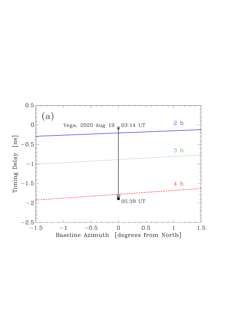
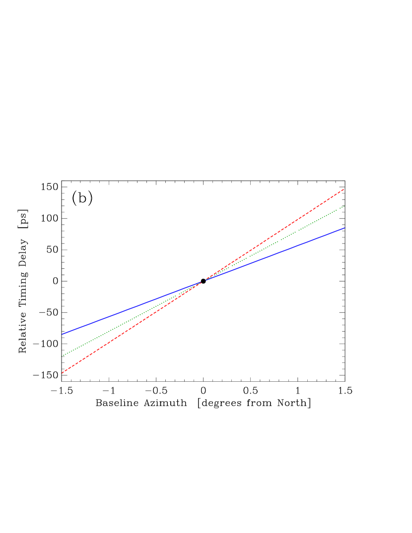
Figure 4: (a) The timing delay given by Equation 11 in the case of Vega, observed from New Haven, as a function of the baseline azimuth. Curves are drawn at three different hour angles, 2 h, 3 h, and 4 h, as indicated by the blue solid curve, the green dotted curve, and red dashed curve respectively. The black vertical line indicates the hour angle range during our actual 2020 Aug 19 observation of Vega as an example, with the starting point indicated with the cross and the end point indicated with the filled circle. (b) The relative timing delay, if a north-south baseline is assumed and the timing corrections indicated along the black vertical line are applied for the entire observing sequence, as a function of baseline azimuth. Curves for the same three hour angles are shown, where again the blue solid curve represents an hour angle of 2 h, the green dotted curve represents 3 h, and the red dashed curve represents 4 h.

However, given our observing site, measuring the angle made with north by the telescope baseline each night is a more difficult task. We have identified the direction to north on the pavement using a plumb bob and marking its shadow at solar noon, but the painted markings are about 2 cm wide. When the telescopes are placed, we must sight down along the telescope base to determine the alignment with the paint mark. We estimate that this can typically be done only to within several mm at present. In this arrangement, we therefore have a much larger uncertainty in $b_{E}$ than in the other two components of the baseline.

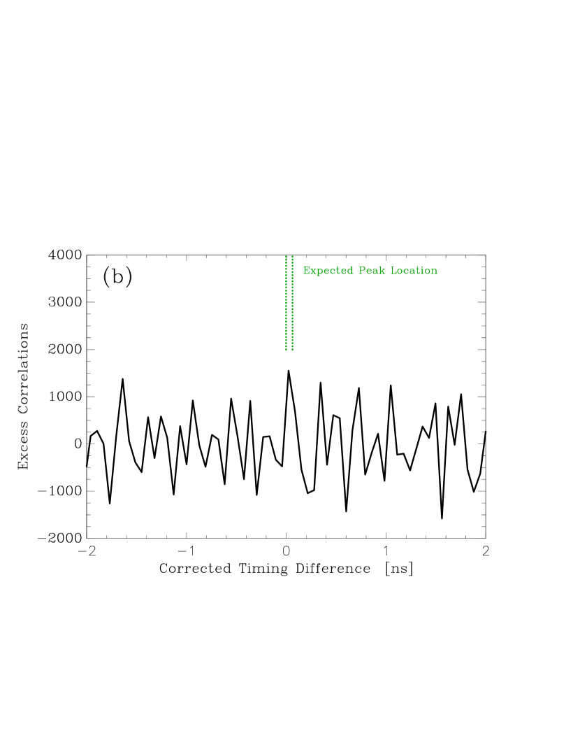
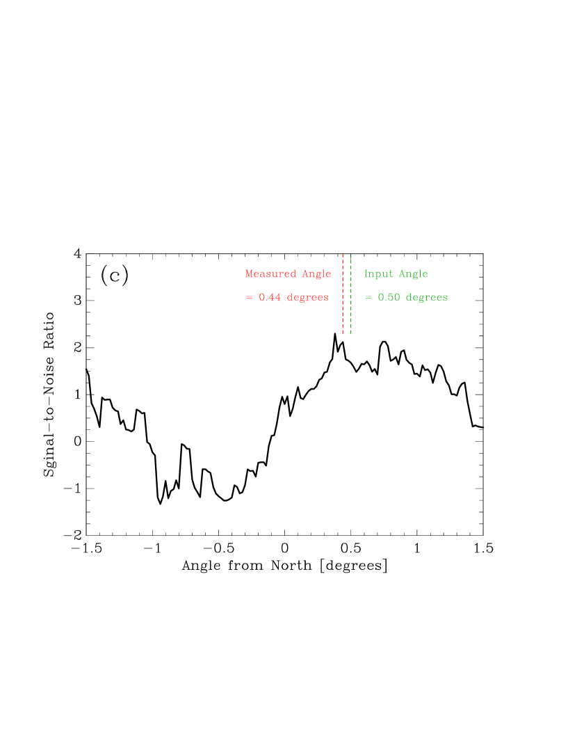
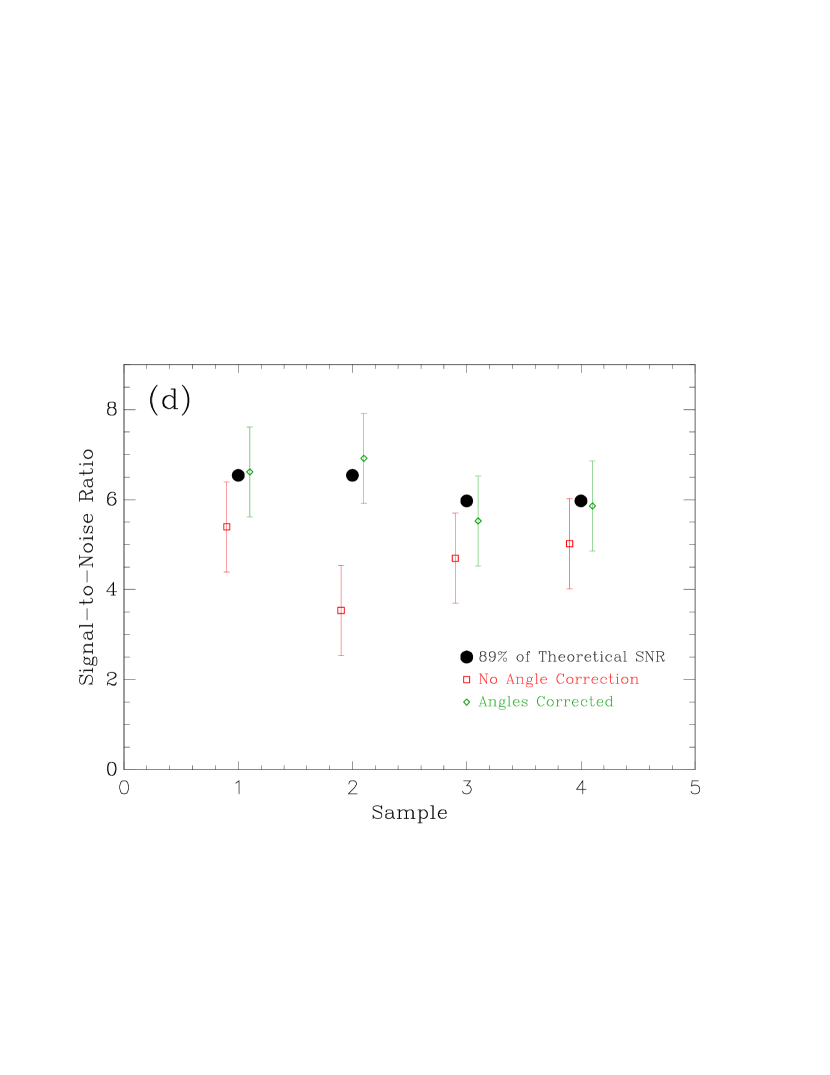
Figure 5: (a) Simulation using the hour angle variation of Vega for 2020 Aug 19 and computing the final, corrected cross-correlation plot assuming a north-south baseline. The SNR here in the expected peak location is 0.80, and the input baseline azimuth was 0.5 degrees. (b) The same data, but with timing corrections made assuming a baseline azimuth of 0.44 degrees. Here the SNR is 2.12. (c) The SNR obtained for the simulation as a function of baseline azimuth. (d) Total SNRs obtained for the samples created from the summation of ten simulations in each case. Black circles indicate 89% of the theoretical correlation (i.e. what we would expect to recover using a timing bin of 64 ps given the result in Figure 3), the red squares indicate the results of the summations if the input angles are not estimated and corrected, and the green diamonds indicate the result of measuring the input angle as in (c) and then co-adding. This process returns the SNR to the level expected.

To study this effect further, we first plot the expected timing difference for a typical observing sequence as a function of the baseline azimuth in Figure 4(a). We use the declination of Vega, latitude of New Haven, and we show the timing delay ($\Delta$ from Equation 11) obtained for three different hour angles. (This range in hour angle is comparable to the observing sequence of Vega on 2020 August 19 that will be discussed in the next section, and that observing sequence is illustrated in the plot.) In Figure 4(b), we show the relative timing difference, if the timing delay were to be corrected based on the assumption of a north-south baseline. At a $0^{\circ}$ baseline azimuth, the relative delay is always zero as the timing shifts used throughout the sequence are always correct, but if the baseline azimuth differs from zero, we see that there is a shift in the final location of the peak, which is more severe at higher hour angles. The effect of this in the final cross-correlation function computed from the timing data of the entire observing sequence is twofold: first, there is an average shift of the cross-correlation peak away from the expected location, and second, the peak is spread out because of the variation in the shift as the hour angle changes.

Next, we constructed a simulation of the data taking process that inputs a baseline azimuth offset and outputs a collection of 25 individual cross-correlations, assumed to be taken over two hours, building in a timing shift throughout that is based on the path of Vega across the sky during that time. We then compute the cross-correlation plot for the entire simulated data set, correcting for $\Delta$. In Figures 5(a) and (b), we show two examples of final cross-correlations obtained in this way, for an input baseline azimuth of $0.5^{\circ}$ and a count rate of 1 MHz. For (a), the timing delays used to correct the data assume a baseline azimuth of $0^{\circ}$, while in (b), the shifts assume a baseline azimuth of $0.44^{\circ}$. We see that, since the first case uses shifts based on an azimuth that is $0.5^{\circ}$ away from the true input angle, the peak appears shifted and spread out. On the other hand, when a value close to the actual azimuth is used to determine the timing corrections, the peak is narrower and appears at the predicted location. We can then vary the baseline azimuth through a range of $-1.5^{\circ}$ to $+1.5^{\circ}$, recomputing the final cross-correlation in each case. Figure 5(c) plots the SNR of these final cross-correlation peaks as a function of baseline azimuth. The original input azimuth is marked (in green), and it can be seen that a broad peak in SNR occurs in this vicinity as more correlation counts are placed at the expected peak location when applying timing shifts generated from those azimuth values. We constructed a routine to estimate the location of this peak from a smoothed version of the SNR curve, and the location of that is also shown in the graph (in red). While typical results show that the input azimuth and the recovered value can differ by up to 0.1-0.2^∘ given the expected SNRs per night, the “tuning” of the azimuth value in software can nonteheless help recover SNR that is lost if the assumption of a 0^∘ azimuth is made. In panel (d) of the figure, we show the results of four samples of simulations (simulation families) done at two different count rates, where measuring the azimuth from the data results in a SNR that is consistent with expectations, once the data is binned in 64-ps increments, whereas if a north-south baseline is assumed, some signal-to-noise is lost.

5 Observations

In this paper, we discuss observations obtained on 16 nights on campus at SCSU and 3 nights where the timing correlator and detectors were taken to Anderson Mesa in Arizona and used with the 1.0-m Hall Telescope and 1.8-m Perkins Telescope at Lowell Observatory.

Table 2: SCSU Observing Summary

Object	Bayer	HR	HD	Date	Tel. Sep.	Filter	Northern	Total Observing
	Desig.			(UT)	(m)	($\lambda_{0}$/$\Delta\lambda$, nm)	Configuration	Time (hr)
Altair	$\alpha$ Aql	7557	187642	2016 Aug 09	3.01	532/3	Tel 2, +1ft, Ch 1	0.61
Arcturus	$\alpha$ Boo	5340	124897	2017 Jun 04	2.099	532/3	Tel 2, Ch 1	0.34
Arcturus	$\alpha$ Boo	5340	124897	2021 Jun 07	2.497	532/1.2	Tel 2, Ch 1	1.10
Arcturus	$\alpha$ Boo	5340	124897	2021 Jun 18	2.488	532/1.2	Tel 2, Ch 7	1.33
Arcturus	$\alpha$ Boo	5340	124897	2021 Aug 07	2.488	532/1.2	Tel 2, Ch 7	0.58
Deneb	$\alpha$ Cyg	7924	197345	2020 Aug 19	2.513	532/3	Tel 2, Ch 0	0.58
Deneb	$\alpha$ Cyg	7924	197345	2020 Aug 25	2.497	532/3	Tel 2, Ch 0	1.24
Deneb	$\alpha$ Cyg	7924	197345	2020 Aug 26	2.493	532/3	Tel 2, Ch 0	1.54
Deneb	$\alpha$ Cyg	7924	197345	2021 Jun 07	2.497	532/1.2	Tel 2, +1ft, Ch 1	0.67
Polaris	$\alpha$ UMi	424	8890	2020 Sep 12	9.167	532/3	Tel 2, Ch 0	2.17
Vega	$\alpha$ Lyr	7001	172167	2016 Jun 23	3.05	532/3	Tel 1, +1ft, Ch 1	0.50
Vega	$\alpha$ Lyr	7001	172167	2016 Jul 27	2.31	532/3	Tel 2, +1ft, Ch 1	0.51
Vega	$\alpha$ Lyr	7001	172167	2016 Sep 14	2.98	532/3	Tel 2, $-$1ft, Ch 0	0.73
Vega	$\alpha$ Lyr	7001	172167	2017 Jun 04	2.099	532/3	Tel 2, +1ft, Ch 1	2.91
Vega	$\alpha$ Lyr	7001	172167	2017 Jun 21	2.331	532/3	Tel 2, Ch 1	1.93
Vega	$\alpha$ Lyr	7001	172167	2017 Aug 09	2.532	532/3	Tel 2, Ch 1	1.39
Vega	$\alpha$ Lyr	7001	172167	2018 May 30	2.502	532/3	Tel 2, +2ft, Ch 7	0.65
Vega	$\alpha$ Lyr	7001	172167	2020 Aug 19	2.513	532/3	Tel 2, +1ft, Ch 1	2.08
Vega	$\alpha$ Lyr	7001	172167	2020 Aug 25	2.497	532/3	Tel 2, +1ft, Ch 1	1.24
Vega	$\alpha$ Lyr	7001	172167	2020 Aug 26	2.493	532/3	Tel 2, +1ft, Ch 1	1.82
Vega	$\alpha$ Lyr	7001	172167	2020 Sep 24	2.496	633/1	Tel 2, +1ft, Ch 1	3.70
Vega	$\alpha$ Lyr	7001	172167	2021 Jun 07	2.497	532/1.2	Tel 2, +1ft, Ch 1	2.09
Vega	$\alpha$ Lyr	7001	172167	2021 Jun 18	2.488	532/1.2	Tel 2, Ch 7	1.83
Vega	$\alpha$ Lyr	7001	172167	2021 Aug 07	2.488	532/1.2	Tel 2, Ch 7	3.00

5.1 On-Campus Observations

The observations taken on-campus have been obtained over a period of nearly 5 years, with the observing site being a relatively secluded area of blacktop near one of our science buildings. A listing of the observations at SCSU is given in Table 2. We have so far only observed with a north-south arrangement of the telescopes, and to place these telescopes, we align them with paint markings that were made for that purpose as described in the previous section. Data were taken on several other nights that are not in Table 2, but on these occasions, either we did not collect enough data to warrant inclusion, or on two occasions, the electronics exhibited noise that was uncharacteristic of the system and which led to strong systematic signatures in the cross-correlation function.

A typical observing sequence consists of placing the telescopes and making the baseline measurements needed for the reductions, checking the collimation of each telescope with a laser collimator, and then sighting on two stars with an eyepiece so that the control units on each telescope can begin tracking the diurnal motion. With the telescopes tracking, we move to the star to be observed, and check the placement of the star in the eyepiece to make sure it is coincident with the center of the finder. We then replace the eyepiece with the SPAD detector and optical harness, and attempt to place the star image on the detector by guiding the telescopes manually. This is done simply by trying to maximize the count rate. Positions of good focus were determined early on in our work with the system, and so the detectors are set at the location of good focus as we mount them, but to further maximize count rates once on the target, we would slightly adjust the focus as needed. Generally, we begin data taking when a count rate of 1 MHz or higher was seen on each channel, and collect data in 5-minute intervals. Because our telescopes have no autoguiders at this stage, it is necessary to manually guide using the telescope hand paddle throughout the observation sequence. As with many alt-az telescopes, our telescopes track poorly near the zenith. Typically, at an altitude of 85^∘ or higher, manual guiding becomes difficult, and one must wait for the star to pass through the meridian to continue observing.

We first discuss the count rates achieved for the on-campus set-up. Figure 6 shows two typical examples of the instantaneous count rates detected, the first for Vega and the second for Polaris. Both observations use the wider 532-nm filter. It is seen here that, although Vega is brighter than Polaris by approximately 2 magnitudes, the average count rates for the two observations are comparable. This is due to the fact that the SPAD detectors and the timing correlator have relatively low maximum count rates that can be read out. For the detector, the cause of this is the relatively long deadtime. However, when reading out in time tag mode, the timing correlator also has a limitation in how fast it can write events. Events are stored in a first-in-first-out (FIFO) buffer as they are transferred to the host computer, and if a large burst of events occurs in a short amount of time, then the FIFO buffer can be overfilled. This causes data taking to stop. There is a good chance of a FIFO overrun in a file if the average count rate exceeds approximately 2 MHz, and so, even on bright objects, the count rate was kept below this value to prevent having to restart files often. (This was done by defocusing and/or moving the star slightly off the center position relative to the detector active area.) In the most recent data taken (in 2021), we have been able to upgrade our host computer, and it handles data faster. Thus, moving forward, we expect to be able to increase our average count rates accordingly. However, at present, we see that count rates in excess of 1 MHz can be obtained on 2nd magnitude stars with SCSI.

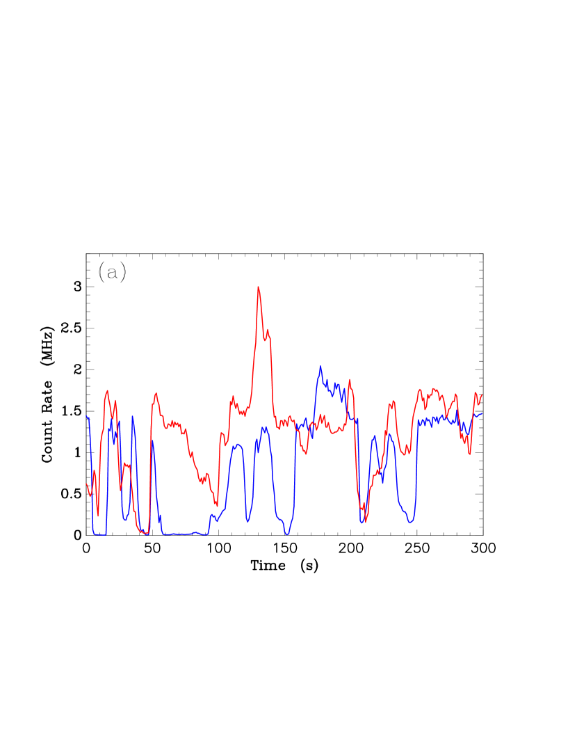
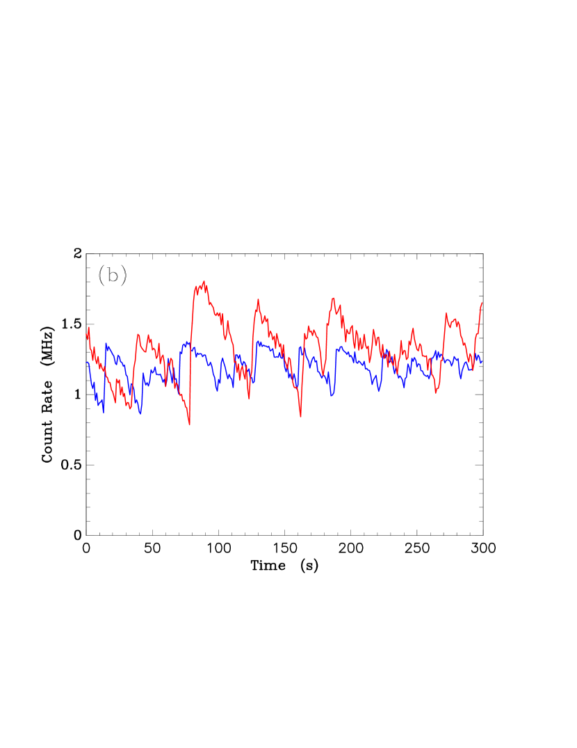
Figure 6: (a) Instantaneous count rates observed for two stars using the wider 532-nm filter. (a) Vega, on 2020 Aug 19, and (b) Polaris observed on 2020 Sep 12. Blue curves represent the count rate in Channel 0 of the correlator, and red curves show the result for Channel 1.

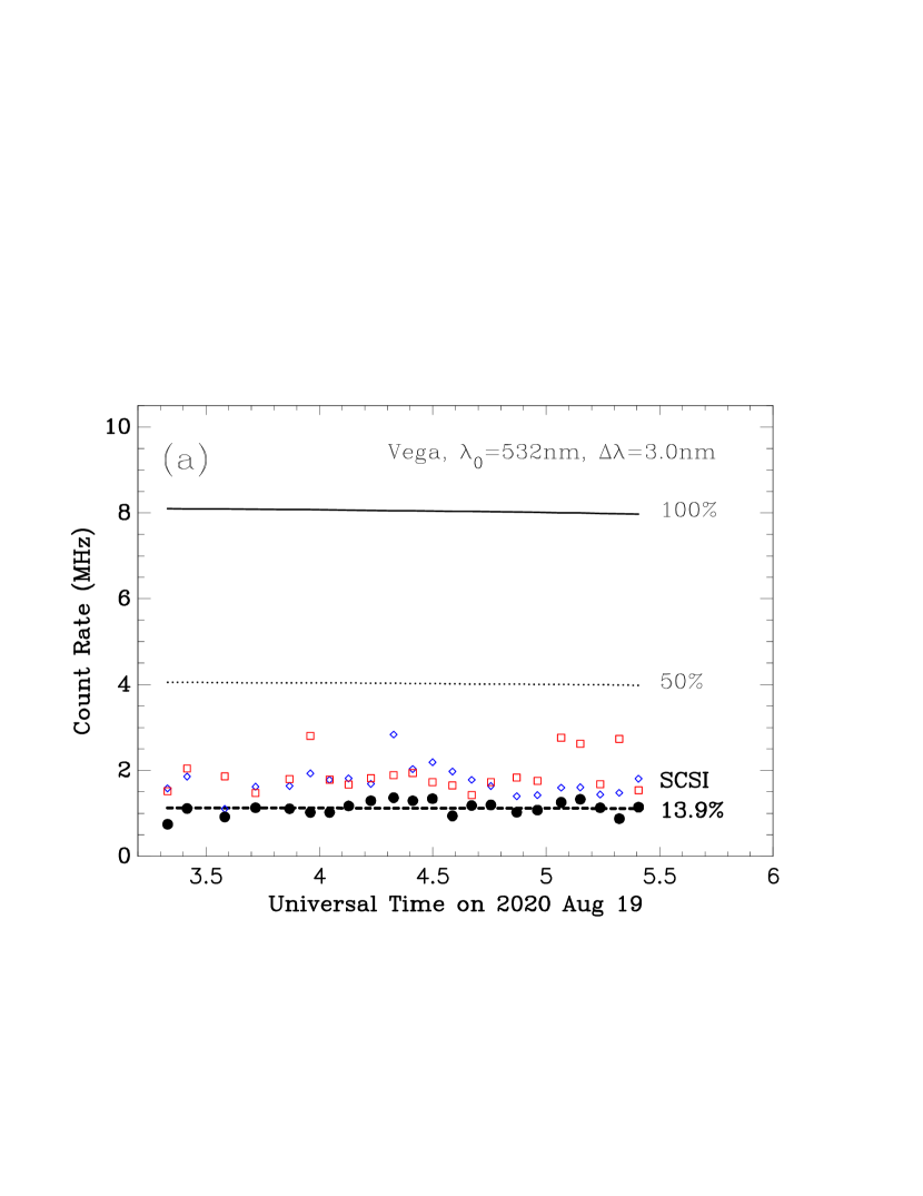
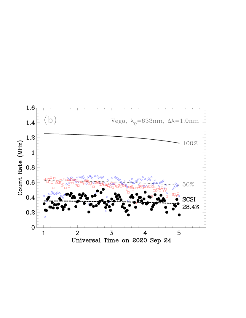
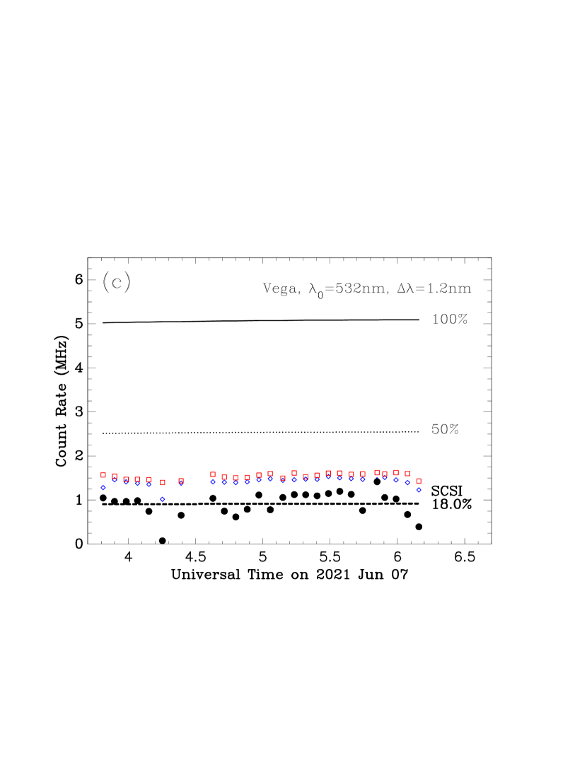
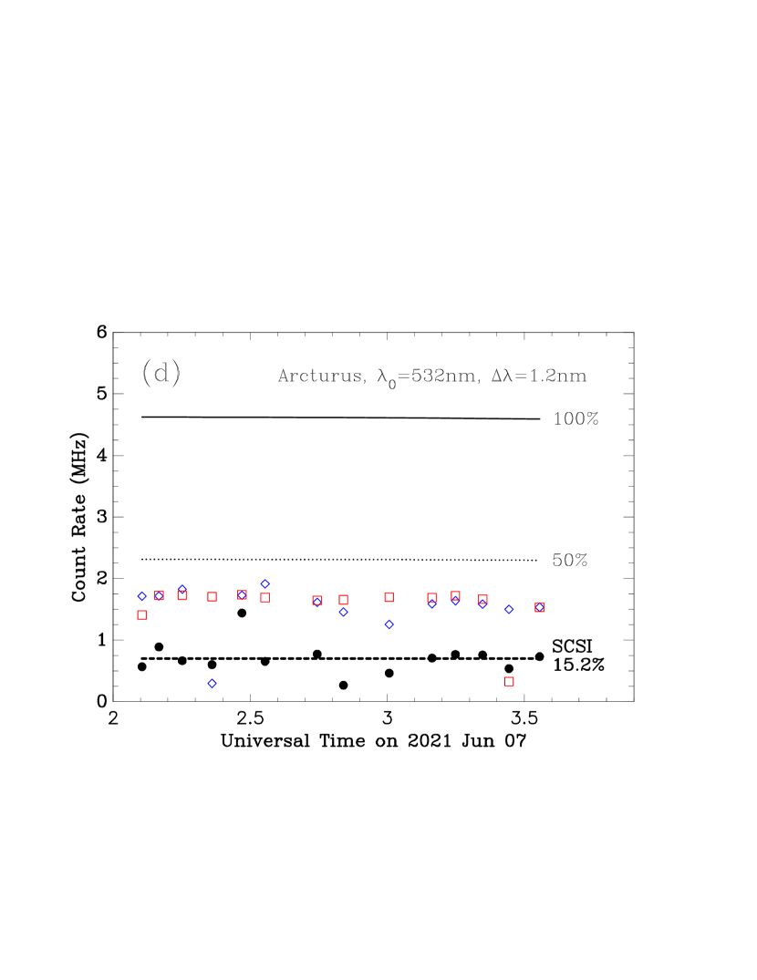
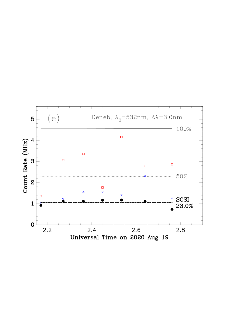
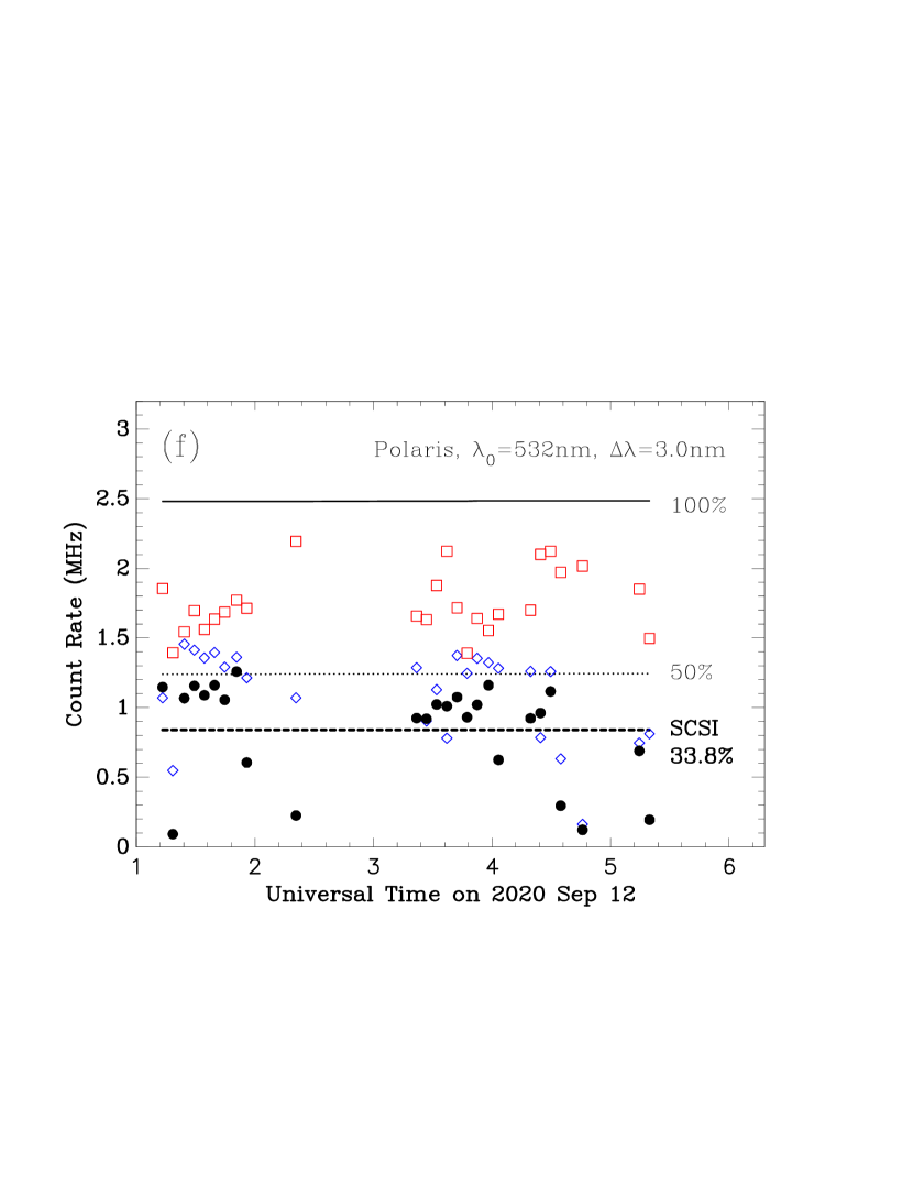
Figure 7: Six examples of count rates obtained for the full sequence of data files using the three different filters and observing four different stars. In all panels, curves are drawn at 100% and 50% of the expected maximum count rate determined from atmospheric and instrumental parameters as described in the text. The blue diamonds and red squares represent the highest average count rate sustained for a 5 second interval in each file for Channels 0 and 1 respectively, and the filled circles represent the average count rate obtained for each file as a whole (including averaging over both telescopes). (a) Vega observed with the wider 532-nm filter. (b) Vega observed with the 633-nm filter. (c) Vega observed with the narrower 532-nm filter. (d) Arcturus observed with the narrower 532-nm filter. (e) Deneb ($\alpha$ Cyg) observed with the wider 532-nm filter. (f) Polaris observed with the wider 532-nm filter.

A second point can be made using the count rates shown in Figure 6. For the observation of Vega, the star was rising toward the zenith, and we can see that the telescopes do not track well enough to keep the star on the detector throughout the file. If we compare the average count rate that we obtain in a file versus the maximum instantaneous rate, there is as much as a factor of two difference. In contrast, with Polaris, we see that the count rates are much more consistent, due to the fact that the star is nearly fixed on the sky, hence the tracking errors develop more slowly over time and it is easier to stay on the target. This indicates that a significant increase in average count rate is possible once better tracking can be made routine.

Figure 7 shows aggregate results for count rates obtained for targets observed on 6 of the 15 nights listed in Table 2. We compare the values recorded with an estimate of the number of photons that should reach the detectors, given the source brightness, telescope aperture size, optical efficiency (including filter width, optical transmission, and atmospheric transmission), and detector quantum efficiency. In each of the six graphs, the expected maximum count rate is shown as the solid black curve. This changes over the course of the night because we incorporate into our calculations the decrease in count rate expected at higher zenith angles. We then fit our count rate data to a similar curve, and derive an overall efficiency estimate for each observation. Typical efficiencies at present are in the 20% range, with some variation due to the effects discussed above.

5.2 Lowell Observations

Observations at Lowell Observatory occurred on three nights, June 6-8, 2015. The observing procedure was largely the same as described above except that, because the telescopes at Lowell are fixed, the baseline did not change from night to night. The observations at Lowell were also at a much larger separation than we have used in the case of the campus telescopes so far. We used the Hall 1.0-m and Perkins 1.8-m telescopes to form the interferometer in this case, which are separated by 53 m on the Anderson Mesa site. The telescope positions are well known, so the issue of placement and its effect on the timing precision is removed. Likewise, telescope pointing and tracking was much less of an issue at Lowell. Detector mounts were constructed for the SPADs for each telescope, but these did not include the two achromats; thus, the filter was not in the collimated beam, leading to a lack of good focus at the detector. Nonetheless, the apertures were large enough to generate count rates for Vega that were comparable to what we achieve with our campus telescopes, roughly 1 MHz per channel. Over the three nights, we obtained about 5 hours of data on Vega in the wider 532-nm filter. The correlator was placed between the two domes and approximately 50 m of cable was stretched from that location to reach the SPAD attached to each telescope.

6 Analysis of the Data

6.1 Data Reduction

To measure the significance of a correlation peak, one would like to determine the total number of correlated events and to compare that with the standard deviation of the number of random correlations detected in the same time interval. There are multiple ways that this might be done, but our approach so far has been to use a binning interval of 64 ps to retain as much signal as possible while keeping the data processing simple and straight-forward. In the future, we hope to continue to improve our reduction tools.

Specifically, we start with a given data file containing the arrival times of photons detected and divide the data into “frames,” that is, smaller intervals that are determined by the rollover time in the internal clock of the timing correlator. Within each frame, we compute timing differences between events in Channel 2 versus Channel 1. These timing differences then populate a histogram of timing differences, which is equivalent to the cross-correlation of the two data streams. Using the timing information of when the file started and ended, we compute the location of the star on the sky at the start of the file, and the shift of its position through the file. This determines the expected location of the correlation peak in the cross-correlation and its smear during the file. Using the latter, we shift cross-correlations from each frame accordingly before coadding them. Finally, a global shift of the cross-correlation is performed to move the starting offset to a fiducial location (usually zero timing delay). Included in the global shift are the known intrinsic channel timing differences as well as the cable differences measured in the laboratory. Repeating these steps for each file in the observing sequence, we can coadd to have a final result for the night on that object. Finally, once all unresolved targets observed on a given night are analyzed in the same way, we establish the baseline azimuth offset from north-south by computing curves similar to simulated result shown in Figure 5. We then boxcar smooth the curve with a width of 0.14 degrees and find the local maximum closest to zero offset in the smoothed version. This gives the final azimuth assumed for a given night.

6.2 Correlation Results

If an intensity interferometry experiment is successful, then the cross-correlation peak should build up with the inclusion of more and more data files. Rewriting Equation 8 in a slightly different way, we obtain

$${\rm SNR}(T)=\frac{\Delta\tau}{2\Delta t}\sqrt{\frac{(r\Delta t)^{2}T}{\Delta t}}.$$ (12)

The right hand consists of two terms, the first of which is the factor multiplying $|V_{12}|^{2}$ in Equation 4; that is, it represents the fraction of correlated photons. Recalling that $(r\Delta t)^{2}$ correlations are produced in a given timing bin of width $\Delta t$, the term under the square root may be seen as the total number of correlations obtained in that timing bin for an experiment of duration $T$. Thus, the SNR is a linear function of the square root of the number of correlations seen in a typical timing bin in the final cross-correlation function for an observing session, where the slope is the fraction of correlated photons. For examaple, a 1-MHz detection rate at each telescope generates $10^{12}$ correlations per second, but these are spread over a large number of 64-ps bins ($\Delta t=64$ ps). Therefore, a typical bin will have 64 counts after cross-correlating 1 second of data. However, if the observing session lasts two hours, then the cross-correlation function will have an average of 460,800 counts per 64-ps bin. Given a correlation fraction of 0.24%, the predicted SNR would be $0.0024\cdot\sqrt{460800}=1.63$. Following this thinking, we can plot the SNR achieved for the observing sequences shown in Table 2. This is shown in Figure 8 for all sources expected to be unresolved at the baselines of our observations. (That is, we do not include observations of Arcturus here because with a known diameter of 21 mas, the star is expected to be partially resolved and to have a reduced correlation.) The plot indicates that the SNRs obtained are generally in the expected range, with the longest observing generating the highest SNRs. We plot these SNR values as a function of the square-root of the mean number of correlations per 64-ps bin; this should be a linear relationship with SNR, with the slope being the correlation fraction. Taking the data at face value and fitting a line to the complete data set regardless of filter, we obtain a slope of $0.00231\pm 0.00039$. The wider of the two 532-nm filters dominates the data set at present, so we find our correlation fraction in line with the expected value discussed in Section 2.

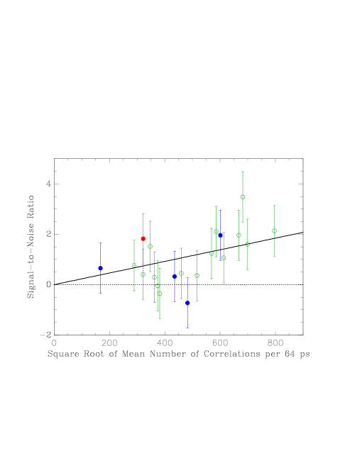
Figure 8: The signal-to-noise ratio of the observations shown in Table 2 as a function of the square root of the mean number of correlations per 64-ps interval. The open circles represent observations taken with the 532/3-nm filter, whereas filled circles represent the two narrower filters, with blue for the 532/1.2-nm and red for the 633/1-nm filter. The linear fit obtained on the entire set of observations is shown as a solid line. The dotted line at zero is meant to guide the eye.

Taking this same set of observations, we can coadd all of the results to generate a single cross-correlation plot. Although this contains data of four separate sources, all are expected to be unresolved from previous diameter determinations. This is shown in Figure 9 in four different representations. Panels (a) and (b) show the cross-correlation result at a resolution of 16 ps. We do not measure the SNR from these plots, but the cross-correlation peak should have a width which is close to 48 ps according to the detecter parameters we have measured. It can be seen in panel (a) that, if the baseline azimuth tuning is not done in the data reduction, there is a spreading out of the peak, whereas when the tuning is applied, the result is that in panel (b). Here, the peak does have the expected width of 3-4 timing samples, as well as the correct position, once all of the timing offsets have been applied. In Figures 9(c) and (d), we show the same data as (a) and (b) respectively, but at a timing resolution of 64 ps. In this case, the correlation should appear as essentially a delta function. The SNR can be estimated by comparing the number of excess correlations in that single sample point with the samples nearby. For the noise calculation, we use the samples between -2 and 2 ns, excluding the three central samples, the middle of which has the correlation peak. We obtain a SNR of 4.70 if the baseline azimuths are not tuned in software, and 6.76 when that tuning is applied.

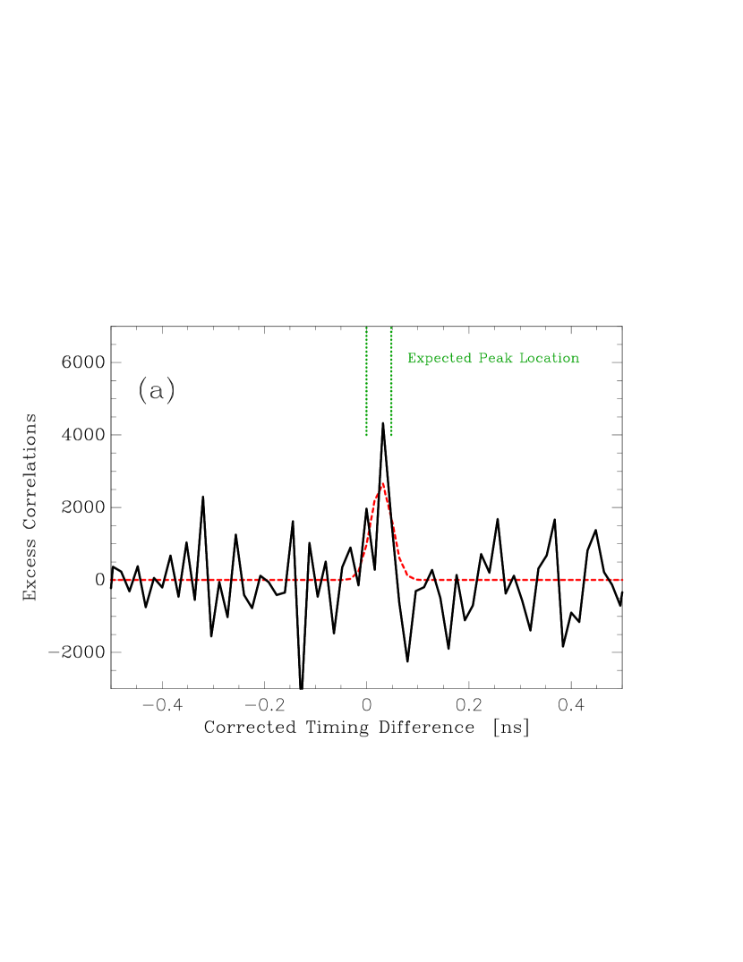
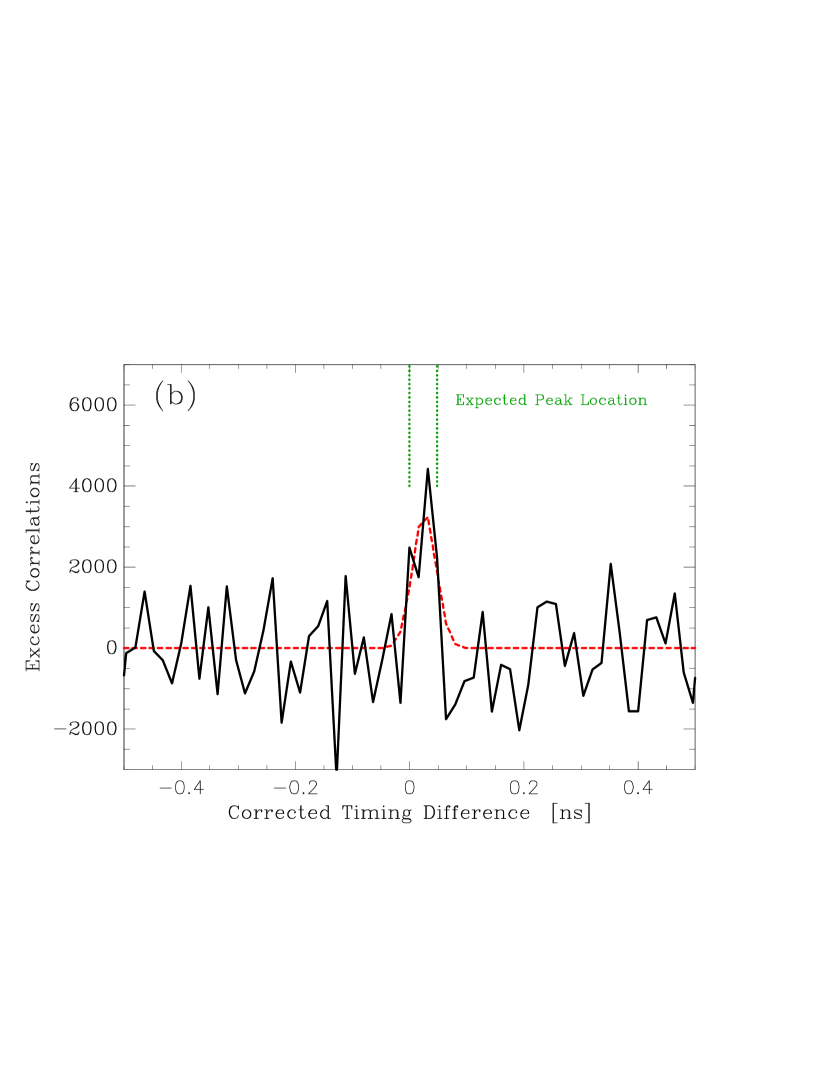
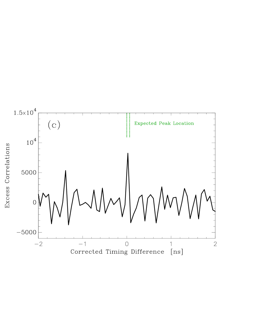
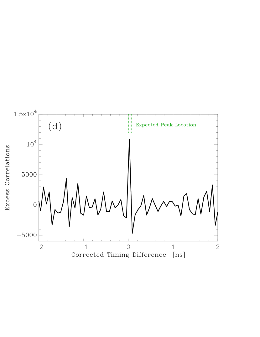
Figure 9: Excess correlations obtained as a function of corrected timing difference when summing all observations where the source is expected to be unresolved. (a) In this plot, no correction for the baseline azimuth has been applied. (b) The same data as in (a), but in this case the baseline azimuth tuning described in the text has been applied for each night prior to summing the results. In these two panels, the plots are drawn at a resolution of 16 ps and the green vertical lines indicate the expected placement of the peak after the timing delays are corrected to the same fiducial. The red dashed curve indicates the best fit Gaussian of FWHM of 48 ps centered on the predicted location. (c) The same data as in (a), but drawn at a resolution of 64 ps. The formal significance of the peak is = 4.70$\sigma$ above the noise. (d) the same data as for (b), but at a resolution of 64 ps. The formal significance here is 6.76$\sigma$. In (c) and (d), the expected location of the peak is again marked.

Finally, we took these data and separated out the measures of each star to create five individual excess correlation plots at the final timing resolution of 64 ps (i.e., the same as in Figures 9[c] and [d]). Setting aside our single observation of Altair ($\alpha$ Aql), Figure 10 shows the results for the four other stars we have observed: Deneb, Polaris, Arcturus, and Vega. The fifth plot is again of Vega, showing the result from Lowell observations only. Given these results, we would expect that our SCSU observations of Vega, Deneb, and Polaris should show a correlation peak, as our observations were taken at baselines generally under 3 m on campus. (Polaris is the exception, where, at a baseline of 9 m the correlation peak may start to decrease.) In contrast, Arcturus has a much larger angular diameter, and the Lowell observations of Vega are at baselines large enough to expect little or no correlation. Although the SNR is low in the plots shown in Figure 10, this trend is indeed seen, where the highest correlations are seen for Deneb and the SCSU observations of Vega, whereas the results for Polaris and Arcturus are consistent with expectations of partial correlation within the uncertainties, and there is no evidence of correlation with the Lowell observations of Vega.

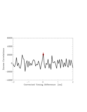
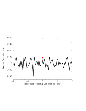
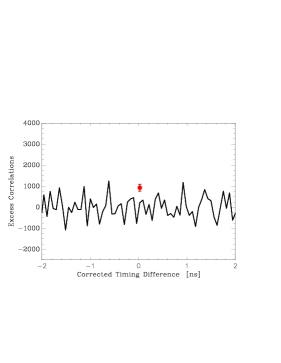
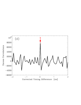
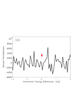
Figure 10: Individual excess correlation plots for each star. (a) Deneb. (b) Polaris. (c) Arcturus. (d) Vega observed at the smaller baselines used at SCSU. (e) Vega observed at the larger baselines at Lowell. In all plots, the timing resolution is 64 ps and the red filled circle represents the predicted location of a full-correlation peak given the mean number of correlations of each data set and assuming a correlation fraction of $0.000231\pm 0.00039$.

Table 3: Previous Angular Diameter Measurements for Star Observed with SCSI

Object	Bayer	HR	HD	$\theta_{LD}$	Instrument	Reference
	Desig.			(mas)
Altair	$\alpha$ Aql	7557	187642	$3.462\pm 0.035$	Mark III	Mozurkewich et al. (2003)
Altair	$\alpha$ Aql	7557	187642	$3.309\pm 0.006$	NPOI	Baines et al. (2018)
Arcturus	$\alpha$ Boo	5340	124897	$21.373\pm 0.247$	Mark III	Mozurkewich et al. (2003)
Deneb	$\alpha$ Cyg	7924	197345	$2.420\pm 0.060$	Mark III	Mozurkewich et al. (2003)
Polaris	$\alpha$ UMi	424	8890	$3.123\pm 0.008$	CHARA	Mérand et al. (2006)
Vega	$\alpha$ Lyr	7001	172167	$3.24\pm 0.07$	Narrabri	Hanbury Brown, Davis & Allen (1974)
Vega	$\alpha$ Lyr	7001	172167	$3.28\pm 0.01$	PTI	Ciardi et al. (2001)
Vega	$\alpha$ Lyr	7001	172167	$3.225\pm 0.032$	Mark III	Mozurkewich et al. (2003)
Vega	$\alpha$ Lyr	7001	172167	$3.280\pm 0.006$	NPOI	Baines et al. (2018)
Vega	$\alpha$ Lyr	7001	172167	$3.33\pm 0.01$	CHARA	Aufdenberg et al. (2006)

6.3 Visibility Measurements

Given that the instrument is detecting excess photon correlations at the expected level, we seek to use Equation 4 to derive information about the visibility as a function of baseline for our observations, in order to make statements about the diameters of the stars observed. For comparison, we show a summary of previous diameter measurements of these four stars in Table 3.

To begin this process, we return to Dyck (1999), where the relationship between the object’s irradiance distribution on the sky is related to its two-dimensional Fourier transform. Defining $u$ and $v$ to be the Fourier conjugate variables to orthogonal spatial coordinates $x$ and $y$ on the image plane, the $(u,v)$ components in the Fourier plane are determined by the following equations involving the observational parameters discussed in Section 4.3:

$$u=(-b_{N}\sin\phi\sin h+b_{E}\cos h+b_{Z}\cos\phi\sin h)/(206265\lambda)$$ (13)

and

$$v=[b_{N}(\sin\phi\sin\delta\cos h+\cos\phi\cos\delta)+b_{E}\sin\delta\sin h-b_{Z}(\cos\phi\sin\delta\cos h-\sin\phi\cos\delta)]/(206265\lambda).$$ (14)

We can use the above to generate a $(u,v)$ plot of observations on a given target each time we observe it. Four examples are shown in Figure 11. We note that, although these sequences trace out an arc in the $(u,v)$-plane, the magnitude of the spatial frequency sampled generally does not change very much. For radially symmetric sources observed over the period of time and sky position that we typically observe them, we are normally acquiring signal at a very narrow range of the magnitude of the spatial frequency vector, $|{\bf u}|$.

This allows us to combine the data on each star and plot it as a function of $|{\bf u}|$. We normalize $|{\bf u}|$ in the typical way as

$$|{\bf u}|=\frac{b}{206265\lambda},$$ (15)

where the units of $|{\bf u}|$ will be cycles per arcsecond. However, to put all our observations on equal footing given the known angular diameters, we can parameterize the relationship between the spatial frequency sampled and the width of the Airy disk in the Fourier plane using the following expression:

$$x=\pi\theta_{\rm LD}|{\bf u}|=\frac{\pi b\theta_{\rm LD}}{206265\lambda}.$$ (16)

Here, following Baines et al. (2018), $\theta_{\rm LD}$ represents the limb-darkened angular diameter of the (radially symmetric) source. The advantage of this parameterization is that, regardless of a star’s angular diameter, the first zero of stellar profile in the Fourier domain will occur in the same place (which would be $x=3.83$ for a perfect Airy pattern, the Fourier transform of a uniform disk). In Baines et al. (2018), those authors use a limb darkening model which depends on a parameter they define as $\mu$, which they measure for each star that they report on. The range of $\mu$ varies from approximately 0.4 to 0.8. In Figure 12(a), we show limb-darkened profiles for these two extremes of $\mu$ using the same formulation as in Baines et al. (2018), and overplot our results for the four stars for which we can measure the squared visibility (the same stars as in Figure 10). These show that as the baseline approaches the first zero of the parameterized stellar profile, the correlation we observe decreases. From this, we conclude that it is possible to measure stellar diameters with our instrument.

In Figure 12(b), we replot the results obtained so far for Vega and Arcturus, where in this case the $x$-coordinate is plotted in cycles per arcsecond. We then change the value of $\theta_{\rm LD}$ so that the visibility curves pass through the upper limit of the error bar for the measurement at highest spatial frequency. For Vega, this data point is the one derived from the observations at Lowell, and we can pass a second pair of curves through the lower limit of the small-$|{\bf u}|$ observation in a similar fashion (this data point being derived from the on-campus observations). The values of $\theta_{\rm LD}$ corresponding to these curves then set limits on the range of the diameters for each star that are currently consistent with our data. For Arcturus, we find $\theta_{\rm LD}>15$ mas, and for Vega, $17$ mas $>\theta_{\rm LD}>0.8$ mas. While the uncertainties are large, these results are nonetheless consistent with the previous measures shown in Table 3.

Our results for Vega may be directly compared with those of a recent experiment observing the same star with the Asiago Stellar Intensity Interferometer (Zampieri et al., 2021). That instrument has a much larger distance between the two telescopes used than at Lowell, but the telescopes used in both cases are comparable in size and the detection and timing instrumentation likewise has similar properties overall. Both their results and ours show a high degree of consistency, giving confidence that the SPAD approach with small telescopes is a viable means with which to conduct intensity interferometry.

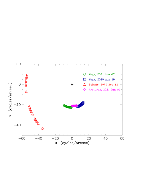
Figure 11: Fourier plane coverage for four representative observing sequences.

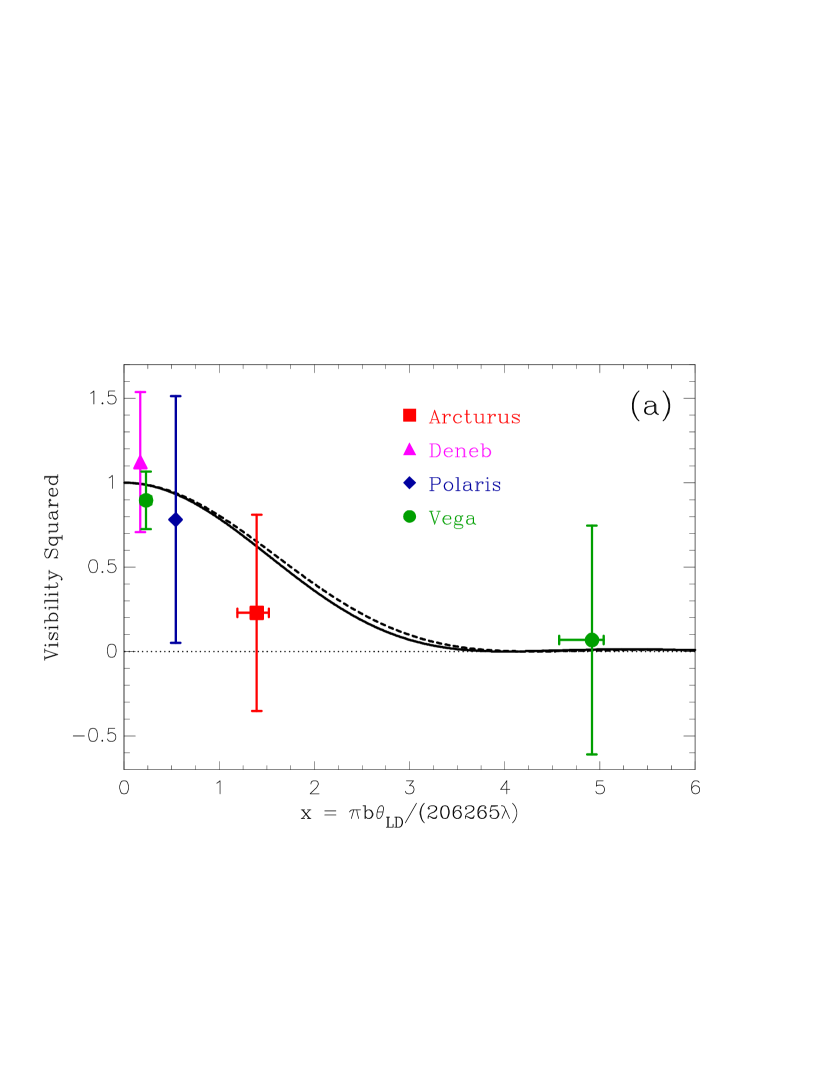
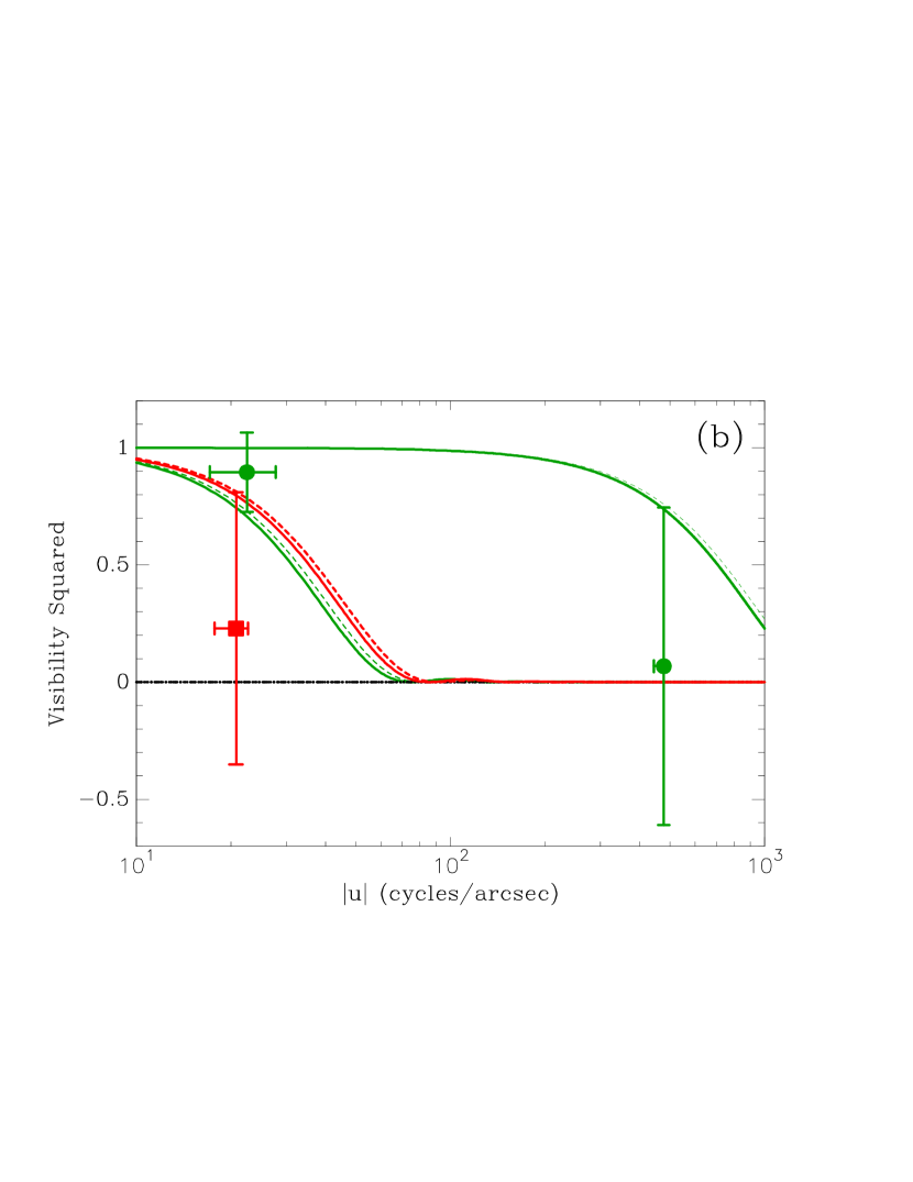
Figure 12: (a) Visibility plot for observations taken to date with SCSI. The solid and dashed curves indicate the two limb-darkened profiles of different $\mu$ value as discussed in the text. (b) The points for Vega and Arcturus are plotted again with the same plot symbol and color, but as a function of the spatial frequency. The solid and dashed lines are the limb-darkened profiles that represent the 1-$\sigma$ lower limit of the angular diameter as discussed for Arcturus and both upper and lower limits for Vega. The abscissa in (b) is plotted on a log scale for clarity.

7 Conclusions and Future Work

We have built a new stellar intensity interferometer which is based on detecting coincident photons at two or more different telescopes using a high-precision timing module and single photon avalanche diode detectors. The timing precision of the instrument is found to be approximately 50 ps. This allows us to use smaller telescopes that have been used in other modern intensity interferometers, although it also requires us to measure our baselines and other instrument parameters very precisely. We have shown that photon correlations are observed at the level expected based on the design of our instrument, and that the data taken to date are consistent with partial correlation within the uncertainties for Arcturus and Polaris. In taking our instrumentation to Lowell Observatory, we observed Vega at a baseline of approximately 50 m using the Hall and Perkins telescopes on Anderon Mesa. This allowed us to add a null result for Vega at that baseline, with large uncertainty. Together these observations permit us to conclude that the angular diameter of Arcturus is larger than 15 mas, and that of Vega between 0.8 and 17 mas. As we have timing correlators with up to 8 channels, our instrument is easily upgraded to include more telescopes; we have already integrated a third telescope identical to the original two and plan to use all three telescopes in ongoing observations moving forward. This will permit us to observe at three baselines simultaneously, making our observations much more efficient.

References

- Abeysekara et al. (2020) Abeysekara, A. U., Benbow, W., Brill, A., et al. 2020, Nature Astronomy, 4, 1164
- Acciari et al. (2020) Acciari, V. A., Bernardos, M. I., Colombo, E., et al. 2020, MNRAS, 491, 1540
- Armstrong et al. (1998) Armstrong, J. T., Mozurkewich, D., Rickard, L. J., et al. 1998, ApJ, 496, 550
- Aufdenberg et al. (2006) Aufdenberg, J. P., Mérand, A., Coudé du Foresto, V., et al. 2006, ApJ, 645, 664
- Baines et al. (2018) Baines, E. K., Armstrong, J. T., Schmitt, H. R., et al. 2018, AJ, 155, 30
- Cammi et al. (2012) Cammi, C., Gulinatti, A., Rech, I., Panzeri, F., & Ghioni, M. 2012, Journal of Modern Optics, 59, 131
- Ciardi et al. (2001) Ciardi, D. R., van Belle, G. T., AKeson, R. L., et al. 2001, ApJ, 559, 1147
- Colavita et al. (1999) Colavita, M. M., Wallace, J. K., Hines, B. E., et al. 1999, ApJ, 510, 505
- Creech-Eakman et al. (2004) Creech-Eakman, M. J., Buscher, D. F., Haniff, C. A., & Romero, V. D. 2004, Proc. SPIE, 5491, 405
- Creech-Eakman et al. (2018) Creech-Eakman, M. J., Romero, V. D., Payne, I., et al. 2018, Proc. SPIE, 10701, 1070106
- Creech-Eakman et al. (2020) Creech-Eakman, M. J., Romero, V. D., Haniff, C. A., et al. 2020, Proc. SPIE, 11446, 1144609
- Davis (1994) Davis, J. 1994, in IAU Symposium 158, Very high angular resolution imaging, ed. J. G. Robertson and William J. Tango (Dordrecht: Kluwer), 135
- Davis et al. (2005) Davis, J., Mendez, A., Seneta, E. B., et al. 2005, MNRAS, 356, 1362
- Dyck (1999) Dyck, H. M. 1999, in Principles of Long Baseline Stellar Interferometry, ed. Peter R. Lawson, JPL Publication 00-009 07/00
- Hanbury Brown (1974) Hanbury Brown, R., The Intensity Interferometer, New York: John Wiley & Sons (1974)
- Hanbury Brown & Twiss (1956) Hanbury Brown, R. & Twiss, R. Q. 1956, Nature, 177, 27
- Hanbury Brown & Twiss (1958) Hanbury Brown, R. & Twiss, R. Q. 1958, Proceedings of the Royal Society of London Series A, 248, 222
- Hanbury Brown, Davis & Allen (1974) Hanbury Brown, R., Davis, J., & Allen, L. R. 1974, MNRAS, 167, 121
- Horch & Camarata (2012) Horch, E. P. & Camarata, M. A. 2012, Proc. SPIE, 8445, 84452L
- Horch et al. (2016) Horch, E. P., Weiss, S. A., Rupert, J. D., et al. 2016, Proc. SPIE, 9907, 99071W
- Horch et al. (2018) Horch, E. P., Weiss, S. A., Rupert, J. D., et al. 2018, Proc. SPIE, 10701,107010Y
- Hummel et al. (1995) Hummel, C. A., Armstrong, J. T., Buscher, D. R., et al. 1995 AJ, 110, 376
- Hutter et al. (1989) Hutter, D. J., Johnston, K. J., Mozurkewich, D., et al. 1989, ApJ, 340, 1103
- Klaucke et al. (2020) Klaucke, P., Pellegrino, R., Weiss, S., & Horch, E. 2020, Proc SPIE, 11446, 114461M
- Klein, Guelman, & Lipson (2007) Klein, I., Guelman, M., & Lipson, S. G. 2007, Applied Optics, 46, 4237
- Labeyrie, Lipson, & Nisenson (2006) Labeyrie, A., Lipson, S. G., and Nisenson, P., An Introduction to Optical Stellar Interferometry, Cambridge: Cambridge University Press (2006)
- Malvimat, Wucknitz & Saha (2014) Malvimat, V., Wicknitz, O., & Saha, P. 2014, MNRAS, 437, 798
- Mandel (1963) Mandel, L. 1963, Progress in Optics, 2, 181
- McAlister et al. (2005) McAlister, H. A., T. A. ten Brummelaar, T. A., Gies, D. R., et al. 2005, ApJ, 628, 439
- Mérand et al. (2006) Mérand, A., Kervella, P., Coudé du Foresto, V., et al. 2006, A&A, 453, 155
- Michelson & Pease (1921) Michelson, A. A. & Pease, F. G. 1921, ApJ, 53, 249
- Mozurkewich et al. (2003) Mozurkewich, D., Armstrong, J. T., Hindsley, R. B., et al. 2003, AJ, 126, 2502
- Nordgren et al. (1999) Nordgren, T. E., Germain, M. E., Benson, J. A., et al. 1999, AJ, 118, 3032
- Pease (1925) Pease, F. G. 1925, PASP, 37, 155
- Pickles (1998) Pickles, A. J. 1998, PASP, 110, 749
- Rivet et al. (2018) Rivet, J.-P., Vakili, F., Lai, O., et al. 2018, Experimental Astronomy, 46, 531
- Rivet et al. (2020) Rivet, J.-P., Siciak, A., de Almeida, E. S. G., et al. 2020, MNRAS, 494, 218
- Schaefer et al. (2020) Schaefer, G. H., ten Brummelaar, T. A., Gies, D. R, et al. 2020, Proc. SPIE, 11446, 1144605
- Shao et al. (1988) Shao, M., Colavita, M. M., Hines, B. E., et al. 1988, A&A, 193, 357
- Tango (2003) Tango, W. J. 2003, Proc. SPIE, 4838, 28
- ten Brummelaar et al. (2005) ten Brummelaar, T. A., McAlister, H. A., Ridgway, S. T. et al. 2005, ApJ, 628, 453
- Weiss, Rupert, & Horch (2018) Weiss, S. A., Rupert, J. D., and Horch, E. P. 2018, Proc. SPIE, 10701, 107010X
- Zampieri et al. (2021) Zampieri, L., Naletto, G., Burtovoi, A., Fiori, M., & Barbieri, C. 2021, MNRAS, 506, 1585