Global Energetics in Solar Flares. XIII. The Neupert Effect and Acceleration of Coronal Mass Ejections

Abstract

Our major aim is a height-time model $r(t)$ of the propagation of Coronal Mass Ejections (CMEs), where the lower corona is self-consistently connected to the heliospheric path. We accomplish this task by using the Neupert effect to derive the peak time, duration, and rate of the CME acceleration phase, as obtained from the time derivative of the soft X-ray (SXR) light curve. This novel approach offers the advantage to obtain the kinematics of the CME height-time profile $r(t)$, the CME velocity profile $v(t)=dr(t)/dt$, and the CME acceleration profile $a(t)=dv(t)/dt$ from Geostationary Orbiting Earth Satellite (GOES) and white-light data, without the need of hard X-ray (HXR) data. We apply this technique to a data set of 576 (GOES X and M-class) flare events observed with GOES and the Large Angle Solar Coronagraph (LASCO). Our analysis yields acceleration rates in the range of $a_{A}=0.1-13$ km s^-2, acceleration durations of $\tau_{A}=1.2-45$ min, and acceleration distances in the range of $d_{A}=3-1063$ Mm, with a median of $d_{A}=39$ Mm, which corresponds to the hydrostatic scale height of a corona with a temperature of $T_{e}\approx 0.8$ MK. The results are consistent with standard flare/CME models that predict magnetic reconnection and synchronized (primary) acceleration of CMEs in the low corona (at a height of $\lower 1.72218pt\hbox{$\;\buildrel<\over{\scriptstyle\sim}\;$}0.1\ R_{\odot}$), while secondary (weaker) acceleration may occur further out at heliospheric distances.

1 Introduction

Eruptive processes, be it a geophysical volcano or a solar flare, imply some causality between the triggering instability and secondary phenomena. The close connection between a solar flare (observed in nonthermal hard X-ray (HXR) emission) and the resulting coronal mass ejection (CME) (observed in white-light and in extreme ultra-violet (EUV) dimming), is generally assumed to follow this causality order. This two-step process may occur in near-simultaneous synchronization, but delays between the two steps are caused by the processes of thermal heating and radiative cooling (e.g., Aschwanden and Alexander 2001; Qiu 2021). While the synchronized occurrence of eruptive flare and CME events appears to be obvious, there are a lot of exceptions, such as flares without CMEs (in the case of non-eruptive or confined events), or CMEs without flares (so-called stealth CMEs; Howard and Harrison 2013). Ambiguities in the association of flares with CMEs occur frequently also, especially when multiple flares occur during a single CME, while the opposite case occurs less frequently. Another difficulty is insufficient time resolution in the cadence of coronagraphs, amounting to $\approx 12$ min for the Large Angle Solar Coronagraph (LASCO) on board of the Solar and Heliospheric Observatory (SOHO). Anyway, the close connection between solar flares and CMEs needs further investigation of these timing issues in a quantitative way. The most novel aspect of this study is the application of the Neupert effect, which predicts acceleration parameters and allows us to test and model the flare/CME relationship from the lower corona out to the heliosphere, even in the absence of HXR data.

The Neupert effect has been discovered in combined soft X-ray (SXR) and microwave emission (Neupert 1968; Kahler and Cliver 1988), and has been dubbed the “Neupert effect” by Hudson (1991). A close correlation between the HXR flux from the Hard X-Ray Burst Spectrometer (HXRBS) onboard the Solar Maximum Mission (SMM) and the time derivative peak of the Geostationary Orbiting Earth Satellite (GOES) has been demonstrated by Dennis and Zarro (1993). The physics of the Neupert effect has been modeled in terms of the thick-target collisional bremsstrahlung process, which acts as the main source of heating and mass supply (via chromospheric evaporation) of the SXR-emitting hot coronal plasma (Veronig et al. 2005). A “theoretical Neupert effect” was established by including variations in emission measure, temperature, radiative cooling losses, conductive cooling losses, and low-energy cutoffs (Veronig et al. 2005; Qiu 2021).

The temporal relationship between CMEs and associated solar flares, observed with GOES and LASCO/SOHO, was found to co-evolve in a few flare/CME events (Zhang et al. 2001; Shanmugaraju et al. 2003; Zhang et al. 2004). Larger statistical studies were performed with GOES and LASCO/SOHO data (up to 3217 CME events) (Moon et al. 2002, 2003), but no strong correlations were found. Significant correlations were found between the CME kinetic energy and the GOES SXR flux (Burkepile et al. 2004), or between the magnitude and duration of CME acceleration (Zhang and Dere 2006; Vrsnak et al. 2007), while other correlations between the duration of CME acceleration, SXR rise time, and SXR peak flux (Maricic et al. 2007), appear to be marginal. Another study with 1114 flares, observed in HXRs with the Burst and Transient Source Experiment (BATSE) onboard the Compton Gamma Ray Observatory (CGRO) and SXRs (GOES), studied the relative timing of the SXR peak time and the HXR fluence, which was found to be consistent with the Neupert effect in about half of the cases (Veronig et al. 2002). It is suspected that the usage of single statistical quantities (such as the HXR end time, SXR peak time, HXR fluence, and HXR end time), neglects important information contained in the light curves (Veronig et al. 2002). However, flaring or non-flaring does not translate into two different types of CMEs (Vrsnak et al. 2005). Tests of the Neupert effect using HXR data (from RHESSI) revealed a synchronization within $\approx 5$ min between the hard X-ray emission (which is a direct indicator of the flare energy release) and the CME acceleration profile (Temmer et al. 2008). More sophisticated tests of the Neupert effect involve data from the Extreme Ultra-Violet Imager (EUVI) and coronagraph COR1 onboard the Solar Terrestrial Relations Observatory (STEREO), which has a high cadence of $\lower 1.72218pt\hbox{$\;\buildrel<\over{\scriptstyle\sim}\;$}2.5$ min), and finds CME acceleration at heights of $h\lower 1.72218pt\hbox{$\;\buildrel<\over{\scriptstyle\sim}\;$}0.4\ R_{\odot}$, as well as CME velocity peaks at heights of $h\lower 1.72218pt\hbox{$\;\buildrel<\over{\scriptstyle\sim}\;$}2.1\ R_{\odot}$ (Temmer et al. 2010).

In this paper we make for the first time use of the Neupert effect to constrain the height-time profile of CMEs propagation in the lower corona, which bridges to the CME trajectory in the heliosphere in a self-consistent way, using GOES and LASCO/SOHO data. We describe the methodology in Section 2, the data analysis and results in Section 3, discussions in Section 4, and conclusions in Section 5.

2 Methodology

This study builds on three previous works on the kinematics and energetics of CMEs, which are based on the EUV dimming method (Aschwanden 2016; Paper IV), self-similar adiabatic expansion (Aschwanden 2017; Paper VI), and the aerodynamic drag force (Cargill 2004; Vrsnak et al. 2004, 2013; Aschwanden and Gopalswamy 2019; Paper VII), while the present study includes the Neupert effect.

2.1 The Neupert Effect

The Neupert effect was first pointed out by Werner Neupert (1968), who noticed that time-integrated microwave fluxes closely match the rising portions of SXR emission curves, which has been demonstrated by others also (e.g., Kahler and Cliver 1988), and was later dubbed the Neupert effect by Hudson (1991). Estimating the time-integrated microwave fluxes from the nonthermal HXR emission, the Neupert effect has been generalized, where the time derivative of the SXR, i.e., $dF_{\rm SXR}(t)/dt$, can be considered as a proxy for the HXR emission $F_{\rm HXR}(t)$ (Dennis and Zarro 1993; Veronig et al. 2002),

$$F_{\rm HXR}(t)\propto{dF_{\rm SXR}(t)\over dt}\ .$$ (1)

The SXR flux $F_{\rm SXR}(t)$ can most conveniently be obtained from GOES 1-8 Å data, which is generally available during the last 46 years (given in units of $Wm^{-2}$). Using the Neupert effect, we can define the peak flux $F_{\rm peak,HXR}$ of the HXR emission,

$$F_{{\rm peak,HXR}}=F_{\rm HXR}(t=t_{\rm peak,HXR})=max[F_{\rm HXR}(t)]\qquad t_{\rm start,GOES}\leq t\leq t_{\rm peak,GOES}\ ,$$ (2)

within the time interval $[t_{\rm start,GOES},t_{\rm peak,GOES}]$. The time profile of a GOES flare is characterized by the start time $t_{\rm start,GOES}$, the peak time $t_{\rm peak,GOES}$, and the end time $t_{\rm end,GOES}$.

The novel application of the Neupert effect here is the model assumption that the start time $t_{\rm start,CME}$ of CME acceleration can be equated to the start time $t_{\rm start,HXR}$ of the HXR flux, which is calculated from the time derivative of the GOES SXR flux (Eq. 1),

$$t_{\rm start,CME}\approx t_{\rm start,HXR}\ .$$ (3)

This assumption can be justified because the start time of a HXR time profile (or light curve) marks the start time of the energy release during a (CME-associated) flare, which is also the start time of the force that launches a CME. While this assertion (Eq. 3) appears to be novel and untested, we will see that the start time $t_{\rm start,GOES}$ of the Neupert-constrained relationship matches the CME start time $t_{\rm start,CME}$ (Eq. 3) in most of the events.

We are using the high time resolution GOES data, which are binned in intervals of $\Delta t=3\ s$. However, in order to have a smooth time profile we average them with a boxcar length of 60 time bins, which corresponds to an effective time resolution of $\Delta t_{smooth}=3$ min, and is sufficient to resolve the shortest flare durations. This implies that the Neupert-constrained flare peak times are also subject to the same accuracy of $\Delta t\approx 3$ min.

2.2 Self-Similar Expansion of CMEs

First we determine the starting height $r_{0}=r(t=t_{0})$ of a CME at the peak time $t_{0}$ of the SXR flux derivative, which is a proxy for the HXR peak time according to the Neupert effect (Eq. 2). We assume a model of self-similar spherical expansion, where the center of the spherical CME bubble starts with a point-like geometry at the start time at a photospheric distance $r=R_{\odot}$ from Sun center. It does not matter if we assume a photospheric or coronal level, since the height difference between the bottom and top of the chromosphere is only about 0.3% of a solar radius $R_{\odot}$. During the spherical expansion, the CME (leading edge) front has a self-similar geometry in all directions, along the plane-of-sky, as well as in any other direction. The location of the CME start can be specified with heliographic longitude and latitude $(l,b)$, and the projected distance of the CME with respect to Sun center at the peak time $t_{0}$ amounts to,

$$r_{0}=r(t=t_{0})=R_{\odot}\ \sin{\sqrt{(l^{2}+b^{2})}}\ ,$$ (4)

which has the minimum limit of $r_{0}=0$ for a halo CME originating at disk center, and $r_{0}=1.0\ R_{\odot}$ for a CME starting at the solar limb.

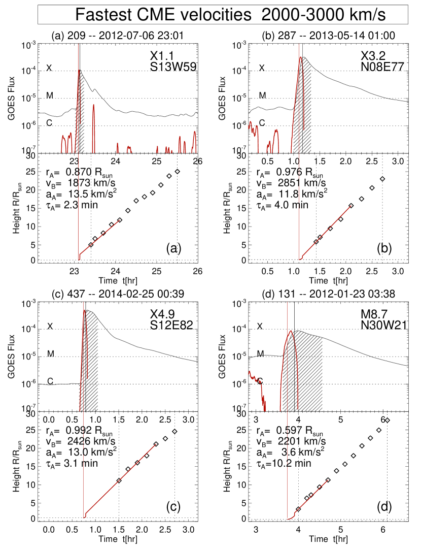
Figure 5: Selection of events with largest CME velocities, otherwise similar to representation in Fig. 1.

In the present study we are using LASCO/SOHO data, but the same procedure can be applied to other full-disk white-light data with heliospheric coverage. The LASCO height-time profiles consist of a time series of height-time measurements $r_{i}=r(t_{i})$, $i=1,...,n$, where the first measurement is taken at a mean altitude of $r_{1}\approx 3R_{\odot}$, and the last is taken at $r_{n}\approx 30\ R_{\odot}$ (see also Fig. 5 in Paper VII). From the LASCO data archive, only the coronagraphs C2 and C3 data have been used for uniformity, because LASCO/C1 was disabled in June 1998.

The Neupert effect predicts the start time $t_{0}$ of the CME from the time derivative of the GOES SXR profile (according to Eq. 3), while the (projected) starting distance $r_{0}=r(t=t_{0})$ is given by the heliographic position (Eq. 4), so that we can add this initial data point $[t_{0},r_{0}]$ to the height-time observations of the LASCO white-light time series $t_{obs,i},i=1,...,n$.

2.3 Kinematic Model of CME Acceleration

The height-time profile $r(t)$ of a CME can in the simplest way be characterized by an initial acceleration phase (during the time interval $t_{A}\leq t\leq t_{B}$) and a subsequent expansion with constant velocity (during the time interval $t\geq t_{B}$), which we define in terms of the acceleration rate profile $a(t)$ being a step-function,

$$a(t)={dv(t)\over dt}=\left\{\begin{array}[]{ll}a_{A}&{\rm for\ }t_{A}\leq t\leq t_{B}\\ 0&{\rm for\ }t\geq t_{B}\\ \end{array}\right.\ .$$ (5)

By integrating the acceleration time profile $a(t)$ we obtain the velocity profile $v(t)$,

$$v(t)=\int_{t_{A}}^{t}a(t)dt=\left\{\begin{array}[]{ll}a_{A}(t-t_{A})&{\rm for\ }t_{A}\leq t\leq t_{B}\\ v_{B}&{\rm for\ }t\geq t_{B}\\ \end{array}\right.\ ,$$ (6)

which essentially yields a linear increase of the CME velocity $v(t)$ during the acceleration phase, and a constant velocity $v(t)$ after the end time of the acceleration phase, with $v(t)=v_{B}$ for $t\leq t_{B}$. Now we can calculate the time integral to obtain the height-time profile, $r(t)$,

$$r(t)=\int_{t_{A}}^{t}v(t)\ dt=\left\{\begin{array}[]{ll}r_{A}+{1\over 2}a_{A}(t-t_{A})^{2}&{\rm for\ }t_{A}\leq t\leq t_{B}\\ r_{1}+v_{B}*(t-t_{1})&{\rm for\ }t\geq t_{B}\\ \end{array}\right.\ .$$ (7)

No linear term $v_{A}(t-t_{A})$ is included because it is more realistic to start acceleration from rest ($v_{A}=0$). The distance $r_{B}$ at the end time $t=t_{B}$ of the acceleration phase follows then from Eq. (7),

$$r_{B}=r_{A}+{1\over 2}a_{A}(t_{B}-t_{A})^{2}\ ,$$ (8)

and the CME velocity $v_{B}=v(t=t_{B})$ follows from Eq. (6),

$$v_{B}=a_{A}(t_{B}-t_{A})\ .$$ (9)

This final CME velocity $v_{B}$ after the end of the acceleration phase can then be obtained from the white-light data $[r_{1},r_{2},...,r_{i},...,r_{n}]$ at the times $[t_{1},t_{2},...,t_{i},...,t_{n}]$,

$$v_{B}={(r_{i}-r_{1})\over(t_{i}-t_{1})}\ ,$$ (10)

where the variable $r_{i}=r(t=t_{i})$ can be arbitrarily selected among the observables $i=2,...,i,...,n$. In principle one could choose a linear regression method, or a polynomial fit, but our tests indicate that the choice of the fitting range leads to larger uncertainties than the formal error of the linear regression or polynomial fit method. Here we choose a value of $i=5$, which is a suitable compromise between data noise reduction (which affects the extrapolation most for $i=2$) and the detection of nonlinear trends (which affects the extrapolation most for $i=n$).

From the expression of $v_{B}$ (Eq. 9) we obtain the acceleration parameter $a_{A}$,

$$a_{A}={v_{B}\over(t_{B}-t_{A})}={v_{B}\over\tau_{A}}\ ,$$ (11)

from which the other parameters can be derived, such as $r_{B}$ (Eq. 8) and $v_{B}$ (Eq. 9).

The Neupert model provides the peak time $t_{0}$ of acceleration and the duration of acceleration, $\tau_{A}=(t_{B}-t_{A})$, which defines the start time $(t_{A})$ and end time $(t_{B})$ of the acceleration phase,

$$t_{A}=t_{0}-{\tau_{A}\over 2}\ ,$$ (12)

$$t_{B}=t_{0}+{\tau_{A}\over 2}\ .$$ (13)

Let us summarize the physical parameters of this CME height-time model that consists of an acceleration phase ($t_{A}\leq t\leq t_{B}$) and a propagation phase ($t_{B}\leq t\leq t_{n}$), where only the time range of ($t_{1}\leq t\leq t_{n}$) can be fitted, depending on the range of available white-light data. Thus we have 6 time markers ($t_{A},t_{0},t_{B},t_{1},t_{i},t_{n}$), 6 distances from Sun center ($r_{A},r_{0},r_{B},r_{1},r_{i},r_{n}$), one CME velocity ($v_{B}$), and one acceleration rate ($a_{A}$). The observed data variables are presented in Figs. (1-6) and Tables (1-3), the theoretical model is shown in Fig. (7), and the analyzed distribution functions and correlations are shown in Figs. (8-9).

3 Data Analysis and Results

3.1 Observations

In the previous studies (Papers IV and VI) we analyzed all 399 GOES $\geq$ M1.0 class flare events observed during the first 3.5 years of the SDO mission (2010 June 1 - 2014 January 31), which we expanded to 576 events (2010 June 1 - 2014 November 16) in Paper VII and in this study here. From the LASCO data we extract height-time profiles that encompass the GOES 1-8 Å flare durations. The LASCO/SOHO catalog (https://cdaw.gsfc.nasa.gov/CME$\_$list) is based on visually selected CME events, and is created and maintained by Seiji Yashiro and Nat Gopalswamy (Yashiro et al. 2008; Gopalswamy et al. 2009, 2010). The LASCO catalog provides height-time profiles $r(t)$ with a typical cadence of $\Delta t_{\rm LASCO}t\approx 12$ min, while we smoothed the GOES time profiles with a box car of $\Delta t_{\rm GOES}=3$ min. The entire data analysis is carried out with an automated CME detection algorithm without any human interaction.

3.2 Examples of Data Analysis

From the total sample of 576 analyzed events we select six special categories of CME events that are presented in Figs. 1-6 and in Table 1, rendering four examples in each group. The full dataset of 576 analyzed events is tabulated in Table 2, available as a machine-readable file.

Group A: Largest (GOES X-class) flares (Fig. 1): This first group of four events represents the largest GOES flares, which range from GOES class X3.3 to X6.9 for the four events shown in Fig. 1. The largest event # 61 (Fig. 1a) has a GOES class X6.9, exhibiting a single-peaked GOES light curve above a background level of GOES C class (black curve in Fig. 1a), and the time derivative of the GOES light curve shows a single-peaked curve too (red curve in Fig. 1a), which defines the Neupert-constrained CME peak time $t_{0}$ (vertical red line). The GOES flare (indicated with a hatched area in Fig. 1a), as cataloged by NOAA, has a start time of 2011-08-09 07:48 UT, a peak time of 08:05 UT, and an end time of 08:08 UT, which defines the flare duration, $\tau_{\rm flare}=(t_{\rm end}-t_{\rm start})=20$ min. The times are given here in units of hours relative to the midnight of the corresponding day. The LASCO detection time range (as indicated with vertical dotted lines), is $t_{1}=t_{\rm start,LASCO}=8.20$ hr, and $t_{n}=t_{\rm end,LASCO}=10.70$ hr. The initial location of the CME is at a distance of $r_{0}=0.95\ R_{\odot}$, based on the flare location with heliographic position N20W69 (Eq. 4). The start time $t_{0}$ of the CME is obtained from the peak of the time derivative of the GOES light curve, evaluated in the time interval between $t_{\rm GOES,start}$ and $t_{\rm GOES,peak}$, following the rule of the Neupert effect. We also measure the duration of the CME acceleration from the full width at half maximum (FWHM) of the time derivative peak, which amounts here to $\tau_{A}=2.4$ min. Note that the duration of CME acceleration ($\tau_{A}=2.4$ min) is much shorter than the GOES flare duration ($\tau_{\rm flare}=20$ min) (as defined by NOAA). The final velocity at $t=t_{n}$ of the CME amounts to $v_{B}=1830$ km s^-1, and the acceleration rate is $a_{A}=12.8$ km s^-2.

The next largest event is of GOES class X5.4 (Fig. 1b), which exhibits an acceleration duration of $\tau_{A}=5.8$ min, a final CME velocity of $v_{B}=2813$ km s^-1, and an acceleration rate of $a_{A}=8.1$ km s^-2. There are actually four peaks visible in the time derivative of the SXR flux, but since the main peak coincides closely with the first detection time of the CME, we consider this CME event as unambiguously associated with the near-simultaneous GOES flare.

The third event (Fig. 1c) shows a relatively late detection of the CME after a delay time of $(t_{1}-t_{A})=1.507-0.740=0.77$ hr) and at a distance of $d_{A}=(r_{1}-r_{A})=11.170-0.992=10.2\ R_{\odot}$. This example demonstrates that our linear extrapolation scheme is fairly robust in determining the CME start time that is assumed to coincide with the start of the flare acceleration time $t_{A}$, even when the CME detection occurs late.

The fourth event is of GOES class X3.3 (Fig. 1d) and indicates a deceleration of the CME velocity $v(t)$ during the detection of white-light data (in the entire time interval from $[t_{1},t_{n}]$), while the range $[t_{1},t_{5}]$ that we use in our extrapolation scheme (Eq. 10) indicates an initially steeper slope, and thus implies a higher velocity. Thus, this example illustrates how the accuracy of the CME velocity $v_{B}$ depends on the choice of the fitting range.

Group B: Smallest GOES M-class flares (Fig. 2): The four smallest GOES M-class flares reach systematically lower altitudes than the large X-class flares during the LASCO detection time window, i.e., $r_{2}\approx 5-10\ R_{\odot}$, compared with $r_{2}\approx 30\ R_{\odot}$ for large X-class flares (e.g., Fig. 1). The four examples shown in Fig. 2 all display a small CME velocity of $v_{B}\approx 200-500$ km s^-1, which appears to be typical for weak GOES class flares (of $\approx$ M1 class).

Examining the extrapolated height-time profiles $r(t)$ in Fig. 2 we notice that they exhibit various degrees of initial “jumps” at the beginning of their profile $r(t)$, from small jumps (event #293; Fig. 2d) to large jumps (event #221; Fig. 2b). Such jumps could occur due to four possible reasons: (i) The initial expansion is much faster than later on during the (heliospheric) expansion (similar to the cosmological inflationary model); (ii) Stealth CMEs that start at an altitude of $r\approx 3-5\ R_{\odot}$; (iii) The CME-associated flare started earlier than identified with our automated detection method, which searches within a finite time window of $[t_{0}-2.0,t_{0}+0.5]$ hr; (iv) Erroneous detection or confusion of white-light CME observations, especially for asymmetric halo CMEs. The inflationary scenario (i) would require two different driver mechanisms or a rapid change in the expansion rate. A stealth-CME scenario (ii) requires an invisible driver, and options (iii) and (iv) imply unlikely large errors in the reported height-time plots of LASCO, so it is not obvious how to explain this phenomenon.

Group C: Largest CME (detection) distances (Fig. 3): The largest CME detection distances in LASCO data amount to $r_{n}\approx 30\ R_{\odot}$. Since the flare event #146 (Fig. 3a) and #147 (Fig. 3b) occur only $\approx 0.2$ hr apart, they cannot be properly disentangled, but it is possible that two CMEs occur in rapid succession. The height-time plot of this two events is close to linear, which implies an almost constant CME velocity. A similar situation occurs for event $\#406$ (Fig. 3c) and $\#407$ (Fig. 3d), where one single CME is reported (from LASCO data), while multiple GOES flares occur during the same CME event, which demonstrates possible ambiguities in the association of flares with CMEs. The latter two events exhibit a very low velocity, $v_{B}=195$ km s^-1, which seems to accelerate after the initial acceleration phase, most likely indicating a second acceleration phase in the solar wind.

Group D: Longest CME durations (Fig. 4): Case 4d reveals double CMEs where one overtakes a previous CME, similar to the “Cannibalistic CMEs” reported by Gopalswamy et al. (2001). Figs. (4a), (4b), and (4c) all show cases with multiple GOES SXR peaks during a single CME detected in LASCO, indicating that matching of GOES flares with CME events can be ambiguous. Moreover, all four events with the longest CME duration exhibit very low initial CME velocities ($v_{B}=41-104$ km s^-2), similar to the CMEs associated with the smallest GOES flares (Fig. 2), and thus may be subject of the same scenarios discussed in group B.

Group E: Fastest CME velocities (Fig. 5): These fastest CMEs have velocities of $v_{B}\approx 2200-3000$ km s^-1 and are associated with large flares (of GOES class M8.7 to X4.9). All four events shown in Fig. 5 have similar characteristics: high velocities and high acceleration rates ($a_{A}\approx 4-10$ km s^-2).

Group F: Slowest CME velocities (Fig. 6): These slowest CMEs have initial velocities of $v_{0}\approx 130-230$ km s^-1 and are associated with the weakest analyzed GOES flare events, from M1.0 to M1.3 class. However, the NOAA flare time range (hatched areas in Fig. 6) does not coincide with the Neupert peak time identified near the LASCO-detected CME start time, which indicates some ambiguity in the association of CME/flare events.

In summary, these 24 cases presented in Figs. 1-6 show a wide variety of cases and illustrate both success and problems of connecting height-time plots from the corona to the heliosphere. The described 24 events can be considered as a representative sample out of the 576 analyzed flare events. Problems occur when (i) a single CME is detected during multiple GOES flares which leads to ambiguities in the association of flares to CMEs, (ii) when the first white-light measurement of the CME front occurs before the Neupert peak time; or (iii) when an initial acceleration and deceleration phase is temporally not resolved. Nevertheless, besides these few problematic cases, the Neupert model was found to be adequate in most cases. We present some statistical information in the next section.

3.3 Flare/CME Event Statistics

From the total analyzed data set of 576 flare/CME events, a subset of 373 events ($65\%$) have a physical solution that is consistent with the Neupert-constrained model of the flare/CME timing (Table 3).

A fraction of 131 flare/CME events ($23\%$) violates the Neupert rule that the start of the flare phase preceeds the start of the CME acceleration phase, although the time difference often amounts to the time resolution of LASCO data ($\Delta t=3$ min). If we correct those events by eliminating the first time bin, the number of Neupert-consistent flare/CME events improves by 47 events ($8\%$) (Table 3).

Another problem in automated CME detection is the ambiguity between CMEs and flares, affecting 84 cases ($15\%$) in our study. Most of these cases show multiple flare events during a single CME, while the opposite case is rarely observed. Flares without CMEs can occur, especially for non-eruptive or confined flares.

3.4 Statistics of CME Variables

In Fig. (8) we show the size distributions of (logarithmic) CME variables, including the GOES flux $F_{\sl SXR}$ (Fig. 8a), the GOES rise time $t_{rise}=t_{peak,GOES}-t_{start,GOES}$ (Fig. 8b), the duration of CME acceleration $\tau_{A}=(t_{B}-t_{A})$ (Fig. 8c), the CME velocity $v_{B}$ (Fig. 8d), the CME acceleration distance $d_{A}=(r_{B}-r_{A})$ (Fig. 8e), and the CME acceleration rate $a_{A}$ (Fig. 8f). The minimum, median, and maximum values of each distribution is listed in each plot. The distributions of the GOES flux and the acceleration time follow approximately an exponential function, which indicates a random process, while all other distributions follow approximately a (log-normal) Gaussian-like function. The median values can be considered as “typical values”. The median GOES class is M2.0. The SXR rise time is $\tau_{rise}=9.0$ min, which is a factor of three longer than the CME acceleration time $\tau_{A}=3.0$ min. The mean CME velocity is $v_{B}=386$ km s^-1, which agrees with the slow solar wind speed. The median acceleration distance is $d_{A}=39$ Mm, which corresponds to the electron density scale height $\lambda\approx 50$ Mm ($T_{e}$ [MK]), fitting a coronal temperature of $T_{e}\approx 0.8$ MK. The median CME acceleration rate is $a_{A}=2.0$ km s^-2, but varies in the range of $a_{A}=0.1-13.5$ km s^-2.

4 Discussion

The close connection between solar flares and CMEs has been studied in many different wavelengths, especially in SXRs and HXRs for flares, and in white-light and EUV for CMEs. Quantitative relationships are generally expressed by flux time profiles $F(t)$ for flares, and by kinematic time profiles for CMEs, such as height-time profiles $r(t)$, velocity profiles $v(t)=dr(t)/dt)$, and acceleration profiles $a(t)=dv(t)/dt$. The most commonly used timing parameters are the start times $t_{start}$, the peak times $t_{peak}$, the rise times $\tau_{rise}=(t_{peak}-t_{start}$), the CME acceleration time duration $\tau_{A}=(t_{B}-t_{A})$, and the flare duration $\tau_{\rm flare}=(t_{\rm end}-t_{\rm start})$. We discuss the most relevant studies and findings in the following.

4.1 CME Acceleration and Soft X-rays

A close correlation between CME acceleration and solar flare SXR emission has been found and corroborated over the last two decades. Analyzing CME events with LASCO/SOHO and EIT/SOHO data, correlations were found between the time evolution of the CME velocity $v_{\rm CME}(t)$ and the time evolution of the GOES SXR flux $F_{\rm SXR}(t)$ (Zhang et al. 2001, 2004; Shanmugaraju et al. 2003; Maricic et al. 2004, 2007; Burkepile et al. 2004; Vrsnac et al. 2007),

$$v_{\rm CME}(t)\propto F_{\rm SXR}(t)\ .$$ (14)

A similar time evolution between the CME velocity and SXR flux implies also similar peak times in the two types of emission, and perhaps a scaling law between the peak values of the two emissions. Such a scaling law has been suggested from measurements of the two quantities at their peak times $t_{\rm peak}$ (Moon et al. 2002, 2003; Maricic et al. 2007; Vrsnac et al. 2004, 2005, 2007; Zhang and Dere 2006),

$$v_{\rm peak,CME}\propto F_{\rm peak,SXR}\ ,$$ (15)

for which we find a marginal correlation only, e.g., CCC$\approx 0.41$ only (Fig. 9a).

Since the acceleration $a(t)=dv(t)/dt$ is by definition the time derivative of the velocity profile $v(t)$, we also expect the following relationship between the CME acceleration $a_{\rm CME}(t)$ and the GOES time derivative $dv_{\rm CME}(t)/dt$,

$$a_{\rm CME}(t)\propto{dv_{\rm CME}(t)\over dt}\propto{dF_{\rm SXR}(t)\over dt}\propto F_{\rm HXR}\ .$$ (16)

This relationship is related to the Neupert effect (Eq. 1), if the time derivative of the SXR time profile $dF_{\rm SXR}/dt$ is taken as a proxy for the HXR light curve $F_{\rm HXR}(t)$ and the acceleration rate $\alpha_{\rm CME}(t)$. The correlation between the acceleration rate $a_{A}$ and the GOES flux is shown in Fig. (9c), which shows a marginal cross-correlation coefficient of CCC=0.29 and a linear regression fit with a slope of 0.29 (Fig. 9c). The only strong correlations are found between the CME velocity $(v_{B})$ and the CME acceleration distance $d_{A}$ (CCC=0.73; Fig. 9d), and the acceleration distance $d_{A}$ and the CME acceleration duration $\tau_{A}$ (CCC=0.70; Fig. 9b). These strong correlations can be explained by the kinematic relationships $v_{B}=a_{A}\tau_{A}$ (Eq. 9) and $v_{B}=d_{A}/\tau_{A}$.

A so-called “indirect flare-proxy method” has been defined to characterize the temporal relationship between CMEs and flares, based on the assumptions that (i) the rise time of the associated SXR flare equals the CME acceleration time $\tau_{\rm A_{a}}$ (Zhang and Dere 2006),

$$\tau_{\rm rise,SXR}=\tau_{A}\ ,$$ (17)

and (ii) the average velocity in the outer corona equals the velocity increase during the acceleration phase (Zhang and Dere 2006). However, here we find that the SXR rise time $\tau_{\rm rise,SXR}$ is not correlated with the CME acceleration duration $\tau_{A}$ (Fig. 9e). The SXR rise time appears to include preflare activities that are not related to the HXR impulsive phase, which is consistent with the fact that the mean SXR rise time, i.e., ($\tau_{\rm rise,SXR}=9.0$ min (Fig. 8b), is a factor of $\approx 3$ longer than the mean acceleration duration ($\tau_{A}=3.0$ min) (Fig. 8c).

Since not all CMEs are accompanied by solar flares, it was investigated whether flare-associated CMEs and flare-less CMEs have different physical parameters, but it turned out that both data sets show quite similar characteristics, contradicting the concept of two distinct (flare and flare-less) types of CMEs. (Vrsnak et al. 2005).

4.2 CME Acceleration and Hard X-Rays

Now we shift our discussion from SXRs to HXRs. A close synchronization between the CME acceleration profile and the flare energy release, as indicated by the RHESSI HXR flux, was found in several CME events, where the HXR peak time and the CME acceleration start occurs within minutes (Temmer et al. 2008; 2010).

Temmer et al. (2008) analyzed the relationship between fast halo CMEs and the synchronized flare HXR bursts for two events, i.e., the X3.8 GOES class event on 2005 January 17, and the M2.5 GOES class event on 2006 July 6, using HXR data from RHESSI and white-light data from LASCO/SOHO. The HXR energy ranges are $\lower 1.72218pt\hbox{$\;\buildrel>\over{\scriptstyle\sim}\;$}50$ keV, and $\lower 1.72218pt\hbox{$\;\buildrel>\over{\scriptstyle\sim}\;$}30$ keV, respectively. The height-time plots of the distance $r(t)$ from the Sun center, as well as the CME velocity profiles $v(t)$ and acceleration profiles $a_{\rm HXR}(t)$ were derived, which clearly demonstrate that the HXR light curve $F_{\rm HXR}(t)$ from RHESSI is highly correlated with the acceleration $a_{\rm HXR}$ of the CME, as measured from the time derivative of the CME height-time plot, synchronized within $\approx 2$ to 5 minutes.

Another three events (2007 June 3, C5.3; 2007 December 31, C8.3; 2008 March 25, M1.7) were analyzed and compared with numerical simulations in Temmer et al. (2010). The distance $r(t)$ of the CME leading edge was measured from STEREO A data, and HXR time profiles $F_{\rm HXR}(t)$ from $>50$ keV RHESSI data. The usage of STEREO data provided coverage of the coronal range of $r\lower 1.72218pt\hbox{$\;\buildrel<\over{\scriptstyle\sim}\;$}3.0\ R_{\odot}$, which is not available in LASCO data (which is also the case for all LASCO events analyzed here). The improved data analysis method yielded relatively small time differences of $\Delta t$= 0.1, 2.0, and 1.5 minutes between the acceleration peak time and the HXR peak time.

The purpose of this study has a very similar goal as the two previous studies of Temmer et al. (2008; 2010), namely the establishment of the time coincidence between solar flare HXR start times and CME acceleration start times. However, instead of using the HXR data from RHESSI (which has been decommissioned on 2018 August 9), we are using GOES 1-8 Å data here and apply the Neupert effect, which yields a fairly reliable proxy for the HXR peak time as calculated from the time derivative of the SXR time profiles (e.g., from GOES). Our strategy is to extrapolate the height-time profiles of LASCO-observed CMEs to the initial coronal height, which supposedly coincides with the Neupert-predicted HXR timing. Temmer et al. (2008; 2010) claim an accuracy of a few minutes in the relative timing, which corresponds to the typical time resolution of $\Delta t_{\rm LASCO}\approx 3$ min used here. We expect that the time resolution constitutes an upper limit on the observed time scales. Indeed, by measuring the full widhts of half maximum (FWHM) of the time derivatives in the GOES flux time profiles, we obtain a compatible mean value of $\tau_{A}=3.0$ min; (Fig. 8c).

4.3 CME Acceleration Parameters

Our Neupert-constrained model provides four independent parameters of the acceleration mechanism for each flare/CME event, based on the measurement of the peak time $t_{0}=(t_{A}+t_{B})/2$ and the acceleration duration $\tau_{A}=(t_{B}-t_{A})$. This includes the start time $t_{A}$ (Eq. 12), the end time $t_{B}$ of the CME acceleration phase (Eq. 13), the mean acceleration rate $a_{A}$ (Eq. 11, Fig. 8f), and the CME acceleration distance $d_{A}=(r_{B}-r_{A})$, (Fig. 8e). The distributions, median values, and ranges are given in Fig. (8), where we find,

$$\tau_{A,med}=3.0\ {\rm[min]}\ ,\quad 1.2<\tau_{A}<44.5\ [{\rm min}]\ ,$$ (18)

$$a_{A,med}=2.0\ {\rm[km\ s^{-2}]}\ ,\quad 0.1<a_{A}<13.5\ [{\rm km}\ s^{-2}]\ ,$$ (19)

$$d_{A,med}=39\ {\rm[Mm]}\ ,\quad 2.8<d_{A}<1063\ [{\rm Mm}]\ .$$ (20)

Compatible acceleration rates were measured in other data sets: $a_{A}=3$ km s^-2 in an X1.6 flare, and $a_{A}=0.2-0.4$ km s^-2 in a M1.0 flare (Qiu et al. 2004). The determination of such parameters in the acceleration of CMEs, entirely based on the Neupert effect, are obtained with unprecedented statistics here.

4.4 Primary CME Acceleration in Hydrostatic Corona

What new insights does the Neupert model convey? A key result is the spatial location of the CME acceleration, which we find to be confined within a median distance of $d_{A,med}=39$ Mm above the solar photosphere. Incidentally, this spatial scale corresponds closely to the hydrostatic scale height $\lambda$ of the corona in the Quiet-Sun and in coronal hole regions, having a typical value of $\lambda_{T}\approx 47$ Mm for a coronal temperature of $T_{e}\approx 0.8$ MK (e.g., Aschwanden 2004, p.69),

$$\lambda(T_{e})={2k_{B}T_{e}\over\mu m_{H}g_{\odot}}\approx 47\left({T_{e}\over 1\ {\rm MK}}\right)\quad{\rm MK}\ ,$$ (21)

where $k_{B}$ is the Boltzmann constant, $\mu\approx 1.27$ is the mean molecular weight (for a H:He=10:1 ratio), $m_{H}$ is the mass of a hydrogen atom, and $g_{\odot}=2.74\times 10^{4}$ cm s^-2 is the solar gravitation. Thus, our statistical study is consistent with an acceleration height located in the lowest electron density scale height of the hydrostatic corona. If the CME propagates along a streamer, the mean coronal density and temperature $T_{e}$ can easily vary by about a factor of two $(T_{e}\approx 0.5-2.0$ MK), i.e., $d_{A,med}\approx 20-100$ Mm.

4.5 Secondary CME Acceleration Phase in Heliosphere

While our analysis method based on the Neupert effect places the CME acceleration region into a low coronal height of $d_{A,med}\approx 40$ Mm $\approx 0.06\ R_{\odot}$, this does not exclude secondary acceleration at larger heights. The height-time plots of the LASCO data reveal secondary acceleration phases, as well as deceleration phases, in heights of $r\approx 3-30\ R_{\odot}$, which can be recognized by their gradual steepening in this height range. For instance, secondary acceleration are most clearly evident in the events #406 (Fig. 3c), #407 (Fig. 3d), #117 (Fig. 4a), #468 (Fig. 4b), #523 (Fig. 4c), and #39 (Fig. 4d), which mostly contain CMEs that propagated over large distances (Fig. 3) or were observed over the longest durations (Fig. 4). So, there is clear evidence for secondary acceleration further out in the heliosphere, but we focus here on the primary acceleration phase only, which generally is driven by a much higher acceleration rate than the secondary acceleration phase. It is likely that the secondary acceleration phase is strongly controlled by aerodynamic drag effects (Cargill 2004; Vrsnak et al. 2004, 2013; Aschwanden and Gopalswamy 2019). The main effect is that CMEs that come out of the coronal primary acceleration phase faster than the ambient solar wind (which has a typical speed of $v_{B}\approx 400$ km s^-1) (Fig. 8d), will be slowed down to solar wind speed, and vice versa, CMEs with initially slow speeds will be accelerated by the solar wind through the aerodynamic drag force.

4.6 The Neupert Effect

The timing of nonthermal HXR emission provides a crucial test for all eruptive flares and CMEs. The temporal coincidence of flare HXR emission with the start of the CME acceleration implies a causality between the two types of emissions. Nonthermal HXRs are believed to be produced by nonthermal electrons that precipitate from a coronal reconnection site into the chromosphere according to the thick-target model, where they are stopped by Coulomb collisions and build up a high plasma pressure that releases its pressure by driving upflows and CMEs. While HXR time profiles $F_{\rm HXR}$ are proportional to the nonthermal electron flux, the accompanied SXR emission piles up according to the time integral of the flux, which implies that its time derivative is proportional to the flux, as stated in the Neupert effect model. Our test of the Neupert model requires a coincidence between the time derivative SXR flux (being the proxy of the HXR flux) and the extrapolated height-time profile of the CME motion, which was found to be the case in $\approx 65\%$ of the (automatically) analyzed events.

High-temperature plasma ($\lower 1.72218pt\hbox{$\;\buildrel>\over{\scriptstyle\sim}\;$}16.5$ MK) was found to be more likely than low-temperature plasma to exhibit to Neupert effect, in which the time derivative of the SXR emission measure is similar to the light curve of the impulsive hard X-ray emission for the flare (McTiernan et al. 1999). A good correlation between occulted hard X-rays (from RHESSI) and the time derivative of the SXR flux was found in many flares, which confirms the Neupert effect in terms of the thin-target bremsstrahlung model, rather than the thick-target model in non-occulted flares (Effenberger et al. 2017). The Neupert effect has also been tested in UV and SXR wavelengths, but a two-phase heating model was required to obtain agreement with observations (Qiu 2021).

5 Conclusions

In this study we model the acceleration phase of CMEs by means of the Neupert effect, which yields important physical parameters in the energization of flare-associated CMEs, such as the peak time $t_{0}$ of the CME acceleration phase, the duration $\tau_{A}$ of the acceleration phase, the height-time profile $r(t)$, the velocity-time profile $v(t)$, and the acceleration rate $a(t)$ of propagating CMEs. A summary of the conclusions is given in the following.

1. Data analysis and modeling has been applied to a CME catalog of 576 flare/CME events that includes all GOES X- and M-class flares recorded during 2010-2014. Combining information from GOES and LASCO/SOHO data sets we are able to model the kinematics of the CME acceleration and propagation. In this study we attempt to connect the time profiles of coronal SXR emission in flares with the white-light emission of flare-associated CMEs in heliospheric distances in a self-consistent way. The observables consist of CME-observed times $[t_{1},...,t_{n}]$ and projected distances $[r_{1},...,r_{n}]$, which are linearly extrapolated in the intermediate range $[t_{B}\leq t\leq t_{1}]$ and quadratically extrapolated during the CME acceleration phase $[t_{A}\leq t\leq t_{B}]$. The missing link is the determination of the exact timing when a CME is accelerated, which we derive from the peak time $t_{0}=(t_{B}+t_{A})/2$ and width (FWHM) $\tau_{A}=(t_{B}-t_{A})$ in the time derivative $dF_{\rm SXR}(t)/dt$ of the GOES SXR flux, which represent a suitable proxy for the HXR flux profiles $F_{\rm HXR}(t)$, according to the Neupert effect. The search of the peak time of the time derivative is limited to the flare SXR rise time interval $\tau_{\rm rise}$.

2. We find the following medium values and parameter ranges in our statistical sample of $n\lower 1.72218pt\hbox{$\;\buildrel<\over{\scriptstyle\sim}\;$}576$ events, shown in form of histograms in Fig. (8): SXR rise time $\tau_{\rm rise}=9.0$ min $(1.0\leq\tau_{\rm rise}\leq 311.0)$ min; acceleration duration $\tau_{A}=3.0$ min $(1.2\leq\tau_{A}\leq 44.5)$ min; acceleration distance $d_{A}=39$ min $(2.8\leq d_{A}\leq 1063$ Mm); and acceleration rate $a_{A}=2.0$ km s^-2 $(0.1\leq a_{A}\leq 13.5)$ Mm. Note that the acceleration time duration is about three times smaller than the SXR rise time, i.e., $\tau_{A}/\tau_{\rm rise}\approx 0.3$.

3. In order to investigate possible physical scaling laws we plot the cross-correlations of 6 parameter pairs (Fig. 9). The strongest correlations are found for the CME acceleration distance $d_{A}$ versus the CME acceleration duration $\tau_{A}$, with CCC=0.70 (Fig. 9b), and for the CME velocity $v_{B}$ versus the CME acceleration distance $d_{A}$, with CCC=0.73 (Fig. 9d). The CME distance from Sun center is defined here by $d_{A}=r_{B}-r_{A}$, which corresponds to the distance traveled through the acceleration region (in radial direction). If the CME velocities have a relatively small variation, we can understand the first correlation $v_{B}=(r_{B}-r_{A})/(t_{B}-t_{A})\propto d_{A}/\tau_{A}$, from which the second correlation follows also. A marginal correlation (CCC=0.41, Fig. 9a) is found between the CME velocity and the GOES flux, which is similar to an earlier study (Moon et al. 2002). However, only a weak correlation (CCC=0.31) is found between the CME acceleration time and the SXR rise time, which indicates that substantial parts of the SXR emission do not produce HXR emission.

4. The CME propagation distance $d_{A}=(r_{B}-r_{A})$ during the time interval $[t_{B},t_{A}]$, marks the vertical extent of the acceleration region, which is is found to have a median value of $d_{A}\approx 40$ Mm and matches the hydrostatic scale height $\lambda(T)$ of the Quiet-Sun corona for a mean temperature of $T\approx 0.8$ MK. This result implies that CME acceleration occurs in the lowest scale height of the hydrostatic solar corona at $r\lower 1.72218pt\hbox{$\;\buildrel<\over{\scriptstyle\sim}\;$}1.1\ R_{\odot}$, while secondary acceleration possibly observed in the heliospheric path of $r\approx 3-30\ R_{\odot}$ are weaker than the primary acceleration rate in the lower corona.

The Neupert effect serves as a suitable proxy for HXR $F_{\rm HXR}(t)$ and can simply be obtained from the time derivative of the SXR flux $F_{\rm SXR}$. The usage of the Neupert effect is particularly useful in times when no (solar-dedicated) HXR detectors are available, such as presently, after the demise of RHESSI in 2018. However, it remains to be shown how accurately the Neupert proxy represents HXR emission (Dennis and Zarro 1993). Nevertheless, as this study shows, the Neupert effect helps enormously to bridge the coronal to the heliospheric part of propagating CMEs, by using a fully automated data analysis code. Future work may include STEREO data (Temmer et al. 2010), which has a higher temporal cadence and spatial coverage in the lower corona ($r\lower 1.72218pt\hbox{$\;\buildrel<\over{\scriptstyle\sim}\;$}3\ R_{\odot}$) that are occulted in coronagraphs like LASCO/SOHO. Coverage in this distance range is crucial to study acceleration and deceleration by the solar wind, by including aerodynamic drag effects (Cargill 2004; Vrsnak et al. 2004, 2013; Aschwanden and Gopalswamy 2019).

Acknowledgements: Part of the work was supported by NASA contracts NNG04EA00C and NNG09FA40C.

References

Aschwanden, M.J. and Alexander, D. 2001, SolPhys 204, 91.

Aschwanden, M.J. 2004, Physics of the Solar Corona - An Introduction (1st Edition), Springer: New York

Aschwanden, M.J. 2016, ApJ 831, 105, (Paper IV)

Aschwanden, M.J. 2017, ApJ 847:27, (Paper VI)

Aschwanden, M.J. and Gopalswamy, N. 2019, ApJ 877:149, (Paper VII)

Burkepile,J.T., Hundhausen, A.J., Stanger, A.L., St. Cyr, O.C., and Seiden, J.A. 2004, JGR (Space Physics), 3103

Cargill, P.J. 2004, SoPh 221, 135

Dennis, B.R. and Zarro, D.M. 1993, SoPh 146, 177

Effenberger, F., Rubio da Costa, F., Oka, M., Saint-Hilaire P., Liu, W., Petrosian, V., Glesener, L., and Krucker, S. 2017, ApJ 835:124

Gopalswamy, N., Yashiro, S., Kaiser, M. L., Howard, R. A., and Bougeret, J. 2001, ApJ 548, L91

Gopalswamy,N., Yashiro,S., Michalek,G., Stenborg,G., Vourlidas,A., Freeland,S., and Howard,R. 2009, Earth, Moon, and Planets 104, 295

Gopalswamy,N., Yashiro, S., Michalek, G., Xie, H., Maekelae, P., Vourlidas, A., and Howard, R.A. 2010, Sun and Geosphere, 5, 7

Howard,T.A. and Harrison, R.A. 2013, SolPhys 285, 269

Hudson, H.S. 1991, BAAS 23, 1064

Maricic,D., Vrsnak, B., Stanger, A. L., and Veronig, A. 2004, SP 225, 337

Maricic,D., Vrsnak, B., Stanger, A. L., Veronig, A. M., Temmer, M., and Rosa, D. 2007, SolPhys 241, 99

Moon, Y.J., Choe,G.S., Wang,H., Park,Y.D., Gopalswamy,N., Yang,G., and Yashiro,S. 2002, ApJ 581, 694

Moon,Y.J., Choe,G.S., Wang,H., Park,Y.D., and Cheng,C.Z. 2003, JKAS 36, 61

Kahler,S.W. and Cliver,E.W. 1988, SolPh 115, 385

McTiernan, J.M., Fisher, G.H., and Li, P. 1999. ApJ 514:472

Neupert, W.M. 1968, ApJ 153, L59

Qiu,J., Wang, H., Cheng, C.Z., and Gary, D. 2004, ApJ 604:900

Qiu,J. 2021, ApJ 909:99

Shanmugaraju,A., Moon, Y.-J., Dryer, M., and Umapathy, S. 2003, SolPhys 215, 185

Temmer, M., Veronig, A.M., Vrsnak, B., Rybak, J., Gomory,P., Stoiser, S., Maricic,D. 2008, ApJ 673, L95

Temmer, M., Veronig, A.M., Kontar, E.P., Krucker, S., Vrsnak, B. 2010, ApJ 712, 1410

Veronig, A.M., Vrsnak, B., Dennis, B.R., Temmer, M., Hanslmeier, A., and Magdalenic, J. 2002, A&A 392, 699

Veronig,A.M., Brown,J.C., Dennis,B.R., Schwartz,R.A., Sui,L., and Tolbert,A.K. 2005 ApJ 621, 482

Vrsnak,B., Ruzdjak, D., Sudar, D., and Gopalswamy, N. 2004, AA 423, 717

Vrsnak,B., Sudar, D., and Ruzdjak, D. 2005, AA 435, 1149

Vrsnak,B., Maricic, D., Stanger, A. L., Veronig, A. M., Temmer, M., and Rosa, D. 2007, SolPhys 241, 85

Vrsnak, B., Zic, T., Vrbanec, D., Temmer, M., Rollett, T., et al. 2013, SoPh, 285, 295

Zhang, Jie, Dere, K.P., Howard, R.A., Kundu, M.R., and White, S.M. 2001, ApJ 559, 452

Zhang, Jie, Dere,K.P., Howard,R.A., and Vourlidas,A. 2004, ApJ 604, 420

Zhang,J., and Dere, K. P. 2006, ApJ 649, 1100

Table 1: Measurements of timing $[t_{A},t_{B},t_{1},t_{n}]$, distances from Sun center $[r_{A},r_{B},r_{1},r_{n}]$, velocity $[v_{B}]$, and acceleration rate $[a_{A}]$ of CMEs and solar flares based on predictions by the Neupert effect, for 24 selected flares (Table 1 and Figures 1-6).

Fig	Nr	GOES	HELPOS	DATEOBS	$t_{A}$	$t_{B}$	$t_{1}$	$t_{n}$	$r_{A}$	$r_{B}$	$r_{1}$	$r_{n}$	$v_{B}$	$a_{A}$
				yyyymmdd hhmm	[hr]	[hr]	[hr]	[hr]	[$R_{\odot}$]	[$R_{\odot}$]	[$R_{\odot}$]	[$R_{\odot}$]	[km/s]	[km/s2]
1a	61	X6.9	N20W69	2011-08-09 07:48	8.037	8.076	8.202	10.702	0.950	1.139	3.010	24.520	1830	12.778
1b	147	X5.4	N18E31	2012-03-07 00:02	0.256	0.352	0.402	2.301	0.586	1.285	2.360	28.690	2813	8.133
1c	437	X4.9	S12E82	2014-02-25 00:39	0.740	0.792	1.507	2.702	0.992	1.317	11.170	24.590	2426	13.025
1d	344	X3.3	S08E42	2013-11-05 22:07	22.181	22.212	22.601	28.502	0.679	0.733	3.330	20.730	674	5.987
2a	35	C7.3	N10W05	2011-03-09 10:35	11.016	11.080	12.202	14.702	0.194	0.239	3.040	7.100	266	1.143
2b	221	M1.0	S20W23	2012-07-14 04:51	4.895	4.944	5.001	7.101	0.507	0.550	4.740	8.090	333	1.874
2c	426	M1.0	S12W13	2014-02-13 08:05	10.518	10.561	11.601	14.001	0.304	0.326	2.810	6.210	200	1.305
2d	293	M1.0	N12E42	2013-05-31 19:52	19.928	19.987	20.601	23.902	0.691	0.768	2.870	9.970	505	2.368
3a	146	M1.0	N18E32	2012-03-06 22:49	0.256	0.352	0.402	2.301	0.598	1.297	2.360	28.690	2813	8.133
3b	147	X5.4	N18E31	2012-03-07 00:02	0.256	0.352	0.402	2.301	0.586	1.285	2.360	28.690	2813	8.133
3c	406	M1.0	S11E13	2014-02-02 16:24	16.444	16.482	17.401	28.702	0.293	0.312	2.440	28.530	195	1.452
3d	407	M3.1	S11E13	2014-02-02 18:05	16.444	16.482	17.401	28.702	0.293	0.312	2.440	28.530	195	1.452
4a	117	M1.9	S19E36	2011-11-15 12:30	12.636	12.704	12.801	33.701	0.652	0.666	2.950	20.310	80	0.328
4b	468	M1.0	S10W57	2014-05-06 22:01	22.099	22.141	22.294	39.702	0.847	0.854	3.090	15.200	70	0.471
4c	523	M3.9	S13E71	2014-10-20 09:00	3.903	3.941	5.401	20.301	0.952	0.956	3.940	16.220	41	0.299
4d	39	M1.3	N07W41	2011-03-12 04:33	18.642	18.676	20.202	34.701	0.664	0.673	2.500	22.910	104	0.852
5a	209	X1.1	S13W59	2012-07-06 23:01	23.094	23.133	23.402	25.502	0.870	1.057	5.030	25.050	1873	13.459
5b	287	X3.2	N08E77	2013-05-14 01:00	1.102	1.169	1.431	2.701	0.976	1.471	5.840	23.030	2851	11.806
5c	437	X4.9	S12E82	2014-02-25 00:39	0.740	0.792	1.507	2.702	0.992	1.317	11.170	24.590	2426	13.025
5d	131	M8.7	N30W21	2012-01-23 03:38	3.740	3.910	4.001	6.101	0.597	1.564	3.380	27.640	2201	3.596
6a	217	M1.1	S17E38	2012-07-09 23:03	19.813	19.866	21.401	27.501	0.664	0.686	2.600	10.170	161	0.861
6b	124	M1.2	S25E67	2011-12-30 03:03	-0.289	-0.245	1.431	9.901	0.948	0.974	3.330	15.240	228	1.469
6c	306	M1.3	S21W22	2013-10-15 23:31	20.132	20.178	21.418	27.702	0.506	0.522	2.830	10.420	130	0.787
6d	64	M1.2	N18W87	2011-09-05 07:27	2.642	2.668	3.401	10.102	1.000	1.014	2.550	12.040	212	2.258

Table 2: Measurements of timing $[t_{A},t_{B},t_{1},t_{n}]$, altitudes $[r_{A},r_{B},r_{1},r_{n}]$, velocity $[v_{B}]$, and acceleration rate $[a_{A}]$ of CME kinematics. The full table of 576 events is available as a machine-readable file.

Nr	GOES	HELPOS	DATEOBS	$t_{A}$	$t_{B}$	$t_{1}$	$t_{n}$	$r_{A}$	$r_{B}$	$r_{1}$	$r_{n}$	$v_{B}$	$a_{A}$
			yyyymmdd hhmm	[hr]	[hr]	[hr]	[hr]	[$R_{\odot}$]	[$R_{\odot}$]	[$R_{\odot}$]	[$R_{\odot}$]	[km/s]	[km/$s^{2}$]
1	M2.0	N23W47	2010-06-12 00:30	0.937	0.973	1.528	9.719	0.791	0.842	3.090	23.090	546	4.271
2	M1.0	S24W82	2010-06-13 05:30	5.592	5.638	5.901	16.301	0.997	1.021	3.280	19.470	205	1.239
3	M1.0	N13E34	2010-08-07 17:55	18.161	18.359	18.602	23.702	0.593	1.106	3.560	26.870	1005	1.417
4	M2.9	S18W26	2010-10-16 19:07	19.170	19.205	20.202	21.819	0.524	0.549	2.580	5.510	278	2.230
5	M1.6	S20E85	2010-11-04 23:30	-0.101	-0.041	0.201	3.502	0.999	1.030	4.430	8.420	198	0.923
6	M1.0	S20E75	2010-11-05 12:43	-0.100	-0.041	1.430	4.302	0.977	1.002	4.950	9.350	161	0.750
7	M5.4	S20E58	2010-11-06 15:27	15.547	15.604	16.202	20.501	0.878	0.897	2.450	6.450	135	0.661
8	M1.3	N16W88	2011-01-28 00:44	0.942	0.980	1.429	5.301	1.000	1.077	3.000	15.150	784	5.718
9	M1.9	N16W70	2011-02-09 01:23	0.178	0.220	0.401	2.202	0.950	0.969	2.790	4.640	173	1.160
10	M6.6	S21E04	2011-02-13 17:28	17.556	17.604	18.601	22.102	0.365	0.399	2.680	9.350	278	1.600
…	…	…	…	…	…	…	…	…	…	…	…	…	…

Table 3: Statistics of analyzed events.

Total number of analyzed events	576	100%
Events with CME preceding flares	131	23%
Ambiguous flare/CME association	84	15%
Consistent with Neupert model	373	65%

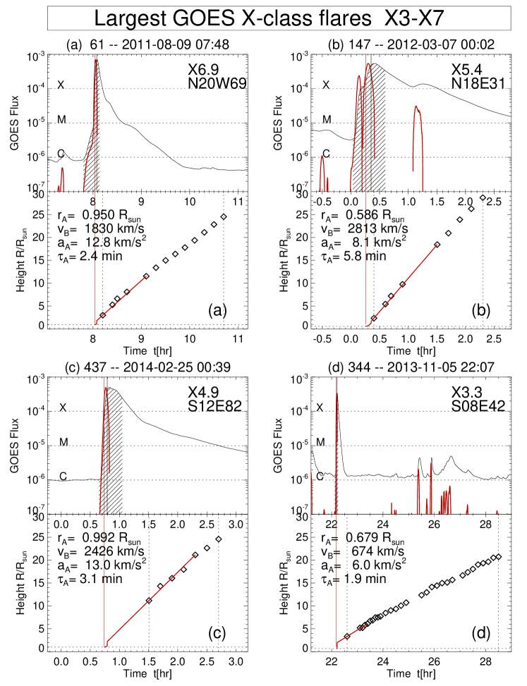
Figure 1: Selection of 4 CME events associated with the largest GOES flares. The GOES 1-8 Å flux is shown with a black curve. The duration of the flare, encompassed by the start time and end time as defined by the NOAA flare classification, is indicated with a dashed area. The time derivative is indicated with red color, and the peak, as defined by the Neupert effect, is marked with a red vertical line. The height-time profile of the LASCO-observed CME is marked with black diamonds, and the first and last observed times with vertical dotted lines.

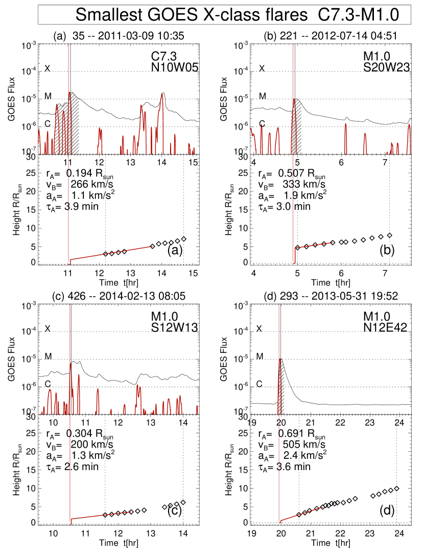
Figure 2: Selection of 4 CME events with smallest GOES flares, otherwise similar to representation in Fig. 1.

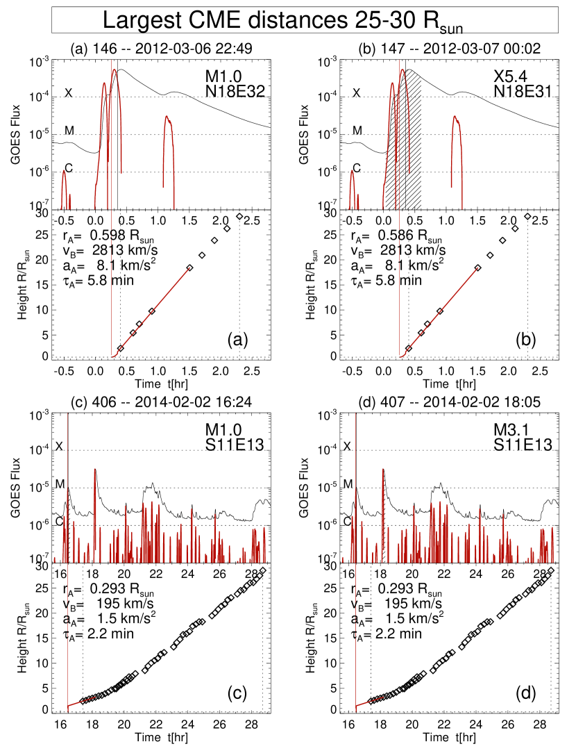
Figure 3: Selection of events with largest CME detection distances, otherwise similar to representation in Fig. 1.

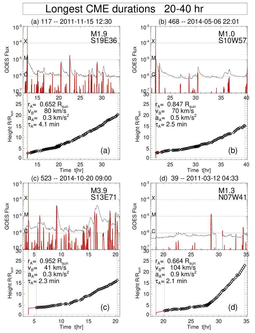
Figure 4: Selection of events with largest CME detection times, otherwise similar to representation in Fig. 1.

Figure 6: Selection of events with slowest CME velocities, otherwise similar to representation in Fig. 1.

Figure 7: The three panels show the analytical functions that describe the height-time profile $r(t)$ (a), the velocity profile $v(t)$ (b), and the acceleration rate $a(t)$ (c). The white-light observations are indicated with diamonds ($t_{1}\leq t\leq t_{n}$), and the acceleration occurs during the time interval ($t_{A}\leq t\leq t_{B}$).

Figure 8: Histograms of the (logarithmic) soft X-ray flux $F_{\rm SXR}$ (a), the GOES flare rise time $\tau_{\bf rise}$ (b), the CME acceleration duration $\tau_{A}=(t_{B}-t_{A})$ (c), the CME velocity $v_{B}=(r_{B}-r_{A})$ (d), the CME acceleration distance $d_{A}=(r_{B}-r_{A})$ (e), and the CME acceleration rate $a_{A}$ (f). The median values of the distributions are indicated with dashed lines, and the minimum and maximum values with dotted lines.

Figure 9: Correlations between the CME velocity and the GOES flux (a), the CME acceleration duration and distance (b), the CME acceleration and the GOES flux (c), the CME acceleration distance and velocity (d), and the CME acceleration time and GOES rise time (e), the CME acceleration velocity and duration (f). The slopes of the linear regression fits and the cross-correlation coefficients are listed in each panel.