J-PLUS: Stellar Parameters, C, N, Mg, Ca and [$\alpha$/Fe] Abundances for Two Million Stars from DR1

Abstract

Context. The Javalambre Photometric Local Universe Survey (J-PLUS) has obtained precise photometry in twelve specially designed filters for large numbers of Galactic stars. Deriving their precise stellar atmospheric parameters and individual elemental abundances is crucial for studies of Galactic structure, and the assembly history and chemical evolution of our Galaxy.

Aims. Our goal is to estimate not only stellar parameters (effective temperature, $T_{\rm eff}$, surface gravity, $\log g$, and metallicity, [Fe/H]), but also [$\alpha$/Fe] and four elemental abundances ([C/Fe], [N/Fe], [Mg/Fe], and [Ca/Fe]) using data from J-PLUS DR1.

Methods. By combining recalibrated photometric data from J-PLUS DR1, Gaia DR2, and spectroscopic labels from LAMOST, we design and train a set of cost-sensitive neural networks, the CSNet, to learn the non-linear mapping from stellar colors to their labels. Special attention is paid to the poorly populated regions of the label space by giving different weights according to their density distribution.

Results. We have achieved precisions of $\delta\,T_{\rm eff}\sim$ 55 K, $\delta\log g\sim 0.15$ dex, and $\delta$ [Fe/H] $\sim$ 0.07 dex, respectively, over a wide range of temperature, surface gravity, and metallicity. The uncertainties of the abundance estimates for [$\alpha$/Fe] and the four individual elements are in the range 0.04–0.08 dex. We compare our parameter and abundance estimates with those from other spectroscopic catalogs such as APOGEE and GALAH, and find an overall good agreement.

Conclusions. Our results demonstrate the potential of well-designed, high-quality photometric data for determinations of stellar parameters as well as individual elemental abundances. Applying the method to J-PLUS DR1, we have obtained the aforementioned parameters for about two million stars, providing an outstanding data set for chemo-dynamic analyses of the Milky Way. The catalog of the estimated parameters is publicly accessible.

1 Introduction

Precise determinations of basic stellar parameters and elemental abundances (hereafter referred to as stellar labels) play a fundamental role in a number of fields, including stellar physics, Galactic structure, the formation and chemical evolution of the Galaxy, and the distribution and properties of dust in the Galaxy. Stellar labels can be determined both spectroscopically and photometrically. These approaches are broadly complementary, each having advantages and disadvantages.

Currently, a number of large-scale photometric surveys, e.g., the SkyMapper Southern Survey (SMSS): DR1.1 – Wolf et al. 2018, DR2 – Onken et al. 2019, the Stellar Abundance and Galactic Evolution (SAGE): Zheng et al. 2018, the Javalambre Physics of the accelerating universe Astrophysical Survey (J-PAS): Benitez et al. 2014, J-PLUS: Cenarro et al. 2019, and the Southern Photometric Local Universe Survey (S-PLUS): Mendes de Oliveira et al. 2019 are producing huge amounts of valuable photometric data for tens of millions of astronomical objects. The medium- and narrow-band filters of these photometric surveys are designed and optimized for precision measurements of key stellar features, opening up a new era of precise and accurate stellar label determinations (see, e.g., Bailer-Jones, 2002; Árnadóttir et al., 2010).

A number of different empirical and theoretical approaches have been developed to determine stellar labels from the use of photometric data. Thanks to the modern large-scale spectroscopic surveys, such as SDSS/SEGUE (Yanny et al. 2009), LAMOST (Deng et al. 2012; Liu et al. 2014), and SDSS/APOGEE (Majewski et al. 2017), and their precise estimates of stellar parameters, advanced (high-quality, large sample size, and good coverage in parameter space) training and calibration data sets are available for inferring stellar labels from photometry. These approaches are now capable of delivering photometric stellar labels with comparable precision to spectroscopy for high-quality photometry. Using a tool based on empirical metallicity-dependent stellar loci, Yuan et al. (2015b, c) estimated photometric metallicites for a half million FGK dwarf stars in SDSS/Stripe 82, with a typical error of $\delta$ [Fe/H] $\sim$ 0.1 to 0.2 dex. Later, Zhang et al. (2021) obtained metallicity-dependent stellar loci for red-giant stars, which were then used to derive metallicities of giants to a precision of $\delta$ [Fe/H] $\sim$ 0.20 to 0.25 dex, and discriminate metal-poor red giants from main-sequence stars based on SDSS photometry.

From corrected broad-band Gaia EDR3 colors alone (Niu et al. 2021b; Yang et al. 2021), Xu et al. (2021) have determined reliable metallicity estimates for a magnitude-limited sample of about 27 million stars down to [Fe/H] = $-2.5$. Considering that the specially designed SkyMapper filters uvgriz of the SMSS are more sensitive to stellar atmospheric parameters than the SDSS filters, Huang et al. (2019) used different polynomials to build empirical relations between atmospheric parameters and photometric colors for red-giant stars, and derived accurate atmospheric parameters (e.g., effective temperature, $T_{\rm eff}$, surface gravity, $\log g$, and metallicity, [Fe/H]) for about one million red-giant stars from SMSS DR1.1. Chiti et al. (2020) describe a grid-based synthetic photometry approach, which was employed by Chiti et al. (2021) to obtain photometric metallicities for over a quarter million giants from SMSS DR2. With the re-calibrated SMSS DR2 and Gaia EDR3, Huang et al. (2021a) have further determined metallicities for over some 24 million stars with a technique similar to the metallicity-dependent stellar loci. Thanks to the strong metallicity sensitivity of the SMSS $uv$ filters, the correction of systematic calibration errors in SMSS DR2, and the use of well-selected training datasets, the achieved precision is comparable to or slightly better than that derived from spectroscopy, for stars with metallicity as low as [Fe/H] $\sim-3.5$.

In addition to empirical metallicity-dependent stellar loci, machine learning methods such as the random forest algorithm (Miller et al., 2015; Bai et al., 2019; Galarza et al., 2021), Bayesian inference (Bailer-Jones, 2011), and artificial neural networks (ANN; Whitten et al. 2019; Ksoll et al. 2020; Whitten et al. 2021), have been suggested to be effective ways to derive precise atmospheric parameters from photometric colors. In particular, ANNs that build an explicit function to map photometric colors to stellar parameters have become a popular tool for estimating atmospheric parameters and elemental abundances. With the J-PLUS photometry, Whitten et al. (2019) proposed SPHINX, a network of ANNs, to derive $T_{\rm eff}$ and [Fe/H] over the range of 4500 K $<T_{\rm eff}<6200$ K, and obtain [Fe/H] down to about $-$3.0 in J-PLUS DR1, with a typical scatter of $\delta$ [Fe/H] $=$ 0.25 dex. Later, Whitten et al. (2021) extended their ANN approach to estimate [C/Fe] to a precision of $\sim 0.35$ dex for SDSS Stripe 82 stars contained in S-PLUS DR2 (Almeida-Fernandes et al., 2021) .

The J-PLUS narrow-band ($\sim 100$ Å) filters are centered on key stellar absorption features; $J0378$ for the CN band, $J0395$ for Ca II H+K, $J0410$ for H$\delta$, $J0430$ for the CH $G$-band, $J0515$ for the Mg $b$ triplet, $J0660$ for H$\alpha$, and $J0861$ for the Ca triplet. Such specially designed filters make it possible to not only determine the basic stellar atmospheric parameters ($T_{\rm eff}$, $\log g$, and [Fe/H]), but also to constrain [$\alpha$/Fe] and elemental abundances such as [C/Fe], [N/Fe], [Mg/Fe] and [Ca/Fe]. Motivated by the above possibilities and their high scientific impact, we have developed a cost-sensitive set of neural networks, CSNet, to derive precise and robust stellar labels ($T_{\rm eff}$, $\log g$, [Fe/H], [C/Fe], [N/Fe], [Mg/Fe], [Ca/Fe],and [$\alpha$/Fe]) for stars in J-PLUS DR1, adopting J-PLUS stars in common with LAMOST and Gaia as training sets. Our models improve the prediction accuracy on the whole by increasing the error penalty for the relatively rare samples of extreme stars.

The paper is organized as follows: Section 2 describes the data used in this work. Section  3 introduces the framework of the proposed method in detail. Section  4 reports the results for the training and the testing samples, as well as comparisons with various validation samples. The resulting catalog of stellar parameters and chemical abundances for stars in JPLUS-DR1 are also presented in Section  4. Section  5 discusses some challenges associated with this work, followed by a summary in Section  6.

2 Data

The dataset used for training and testing CSNet is constructed by stars in common between J-PLUS DR1 (Cenarro et al. 2019), Gaia DR2 (Gaia Collaboration et al. 2018), and LAMOST DR5 (http://dr5.lamost.org, Luo et al. 2015; Xiang et al. 2019), where the first two data sets provide input stellar colors and the last one provides stellar labels ($T_{\rm eff}$, $\log g$, [Fe/H], [C/Fe], [N/Fe], [Mg/Fe], [Ca/Fe] and [$\alpha$/Fe]).

2.1 Stellar colors

J-PLUS is being conducted from the Observatorio Astrofísico de Javalambre (OAJ, Teruel, Spain; Cenarro et al. 2014) using the 83 cm Javalambre Auxiliary Survey Telescope (JAST80) and T80Cam, a panoramic camera of 9.2k $\times$ 9.2k pixels that provides a $2\deg^{2}$ field of view (FoV) with a pixel scale of 0.55 arsec pix^-1 (Marin-Franch et al., 2015). Its unique combination of 5 broad-band ($ugriz$), and 7 medium- and narrow-band filters ($J0378,J0395,J0410,J0430,J0515,J0660,J0861$), optimally designed to extract the rest-frame spectral features (including the Balmer jump region, which covers the molecular CN feature, Ca II H+K, H$\delta$, the CH $G$-band, the Mg $b$ triplet, H$\alpha$, and the Ca triplet) plays a key role in characterizing stellar types and elemental abundances in this work. The J-PLUS observational strategy, image reduction, and main scientific goals are presented in Cenarro et al. (2019).

The first J-PLUS Data Release (DR1) covers 1022 $\text{deg}^{2}$ with 511 pointings in its footprint observed from November 2015 to January 2018 (Cenarro et al. 2019). The 5$\sigma$ limiting magnitudes (3^′′ aperture) in the filters reach a limit of about 21. Using a stellar locus method, López-Sanjuan et al. (2019) have reached a calibration accuracy of 1-2 per cent, larger for bluer filters. Using the stellar color regression method (SCR; Yuan et al. 2015a, Huang et al. 2021b, Niu et al. 2021a, Niu et al. 2021b, Huang & Yuan 2021), by combining the LAMOST DR5 spectroscopy and Gaia DR2 photometry, we have re-calibrated the J-PLUS DR1 data and achieved an accuracy of about 0.5 per cent or better for all the J-PLUS filters (Yuan et al. in preparation). Strongly correlated calibration errors are found in the previous calibration, due to the strong metallicity-dependence of stellar loci for blue filters (e.g., Yuan et al. 2015b, López-Sanjuan et al. 2021) and errors in the 3D dust map and reddening coefficients used (Yuan et al. in preparation). In order to make the best use of the full power of J-PLUS filters, the re-calibrated J-PLUS DR1 data are used in this work. The same data have also been used in star/galaxy/quasar classifications (Wang et al. 2021a), as well as for estimates of basic stellar parameters (Wang et al. 2021b), with a Support Vector Machine technique.

Gaia DR2 (Gaia Collaboration et al. 2018) delivers five-parameter astrometric solutions as well as integrated photometry in three very broad bands: $G$, $B$P (330 – 680 nm), and $RP$ (630 – 1 050 nm), for 1.4 billion sources with $G$ $<$ 21. It provides not only the best astrometric data ever obtained, but also the most precise photometric data. The typical uncertainties in Gaia DR2 measurements at $G$ = 17 are $\sim$ 2 mmag in the $G$-band photometry, and $\sim$ 10 mmag in $BP$ and $RP$ magnitudes (Gaia Collaboration et al. 2018).

With the additional $BP$ and $RP$ magnitudes from Gaia DR2, a total of 13 stellar colors are computed and used in this work, as listed in Table 1. These combinations of colors are believed to contain all the pertinent stellar parameter and elemental-abundance information hidden in the J-PLUS photometry. Reddening corrections have been applied to these colors with empirical reddening coefficients determined with the star-pair technique (Yuan et al. 2013; Yuan et al. in preparation) and $E(B-V)$ reddening values from the SFD98 map (Schlegel et al. 1998). The coefficients are also listed in Table 1.

[b] No. Colors¹ Empirical reddening coefficients 1 $BP-RP$ $\,\,\,\,1.360$ 2 $BP-u$ $-1.379$ 3 $BP-g$ $-0.339$ 4 $RP-r$ $-0.678$ 5 $RP-i$ $-0.033$ 6 $RP-z$ $\,\,\,\,0.439$ 7 $BP-J0378$ $-1.203$ 8 $BP-J0395$ $-1.158$ 9 $BP-J0410$ $-0.953$ 10 $BP-J0430$ $-0.809$ 11 $BP-J0515$ $-0.069$ 12 $RP-J0660$ $-0.454$ 13 $RP-J0861$ $\,\,\,\,0.339$

Table 1: Empirical reddening coefficients for stellar colors.

• $BP$ and $RP$ photometry are from Gaia DR2; $ugriz$, $J0378$, $J0395$, $J0410$, $J0430$, $J0515$, $J0660$, and $J0861$ photometry are from J-PLUS DR1.

The input colors for CSNet are constructed by cross-matching J-PLUS DR1 with Gaia DR2, adopting a matching radius of 1.0 arcsec. Considering that the 6 arcsec aperture measurements of J-PLUS DR1 are used, we require that stars satisfy photo_bp_rp_excess_factor $\leq$ 1.25 + $0.06(BP-RP)^{2}$, slightly stricter than that suggested by Evans et al. (2018), to avoid possible contaminations from nearby sources. To ensure the quality of the photometry, we require that stars satisfy FLAGS $=$ 0. For the training and the testing samples, we further require that photometric uncertainties of the 12 J-PLUS filters are lower than 0.01 mag for the griz filters, 0.02 mag for the $J0410,J0430$ and $J0515$ filters, and 0.03 mag for the $J0378,J0395$, and $J0410$ filters, respectively. With the above contraints, the G magnitude ranges over 11.6 – 16.7 for the training and the testing samples.

2.2 LAMOST stellar labels

The Large sky Area Multi-Object fiber Spectroscopy Telescope (LAMOST; Cui et al. 2012) collects low-resolution (R$\sim$1800) and medium-resolution (R$\sim$7500) spectra in a FoV of 20 $\text{deg}^{2}$. In its fifth Data Release, LAMOST DR5, this survey has delivered more than 8 million stellar spectra with spectral resolution $R=1800$ and limiting magnitude of $r\sim$ 17.8 (Deng et al. 2012; Liu et al. 2014). Stellar effective temperatures, $T_{\rm eff}$, surface gravities, $\log g$, and metallicities, [Fe/H], are derived by the LAMOST Stellar Parameter Pipeline (LASP; Wu et al. 2011).

For the elemental abundances [C/Fe], [N/Fe], [Mg/Fe], [Ca/Fe], and [$\alpha$/Fe], the data-driven Payne (The DD-Payne) results of Xiang et al. (2019) are used. The DD-Payne inherits essential ingredients from both The Payne (Ting et al. 2019) and The Cannon (Ness et al. 2015), and incorporates constraints from theoretical model spectra to ensure physically meaningful abundance estimates. Stars in common between LAMOST DR5 and either GALAH DR2 (Buder et al. 2018) or APOGEE DR14 (Holtzman et al. 2018) were used as the training data set to provide abundances for 16 elements (C, N, O, Na, Mg, Al, Si, Ca, Ti, Cr, Mn, Fe, Co, Ni, Cu, and Ba). For stars with spectral signal to noise ratios $\rm S/N_{g}$ higher than 50, the typical internal uncertainties of the estimated abundances are about 0.05 dex for [Fe/H], [Mg/Fe], and [Ca/Fe], 0.1dex for [C/Fe] and [N/Fe]. The [$\alpha$/Fe] of this catalog was defined as a weighted mean of [Mg/Fe], [Ca/Fe], [Ti/Fe], and [Si/Fe]. Note that for the elemental abundances used in this work, [Mg/Fe] was trained using GALAH DR2, while the others used APOGEE DR14.

2.3 Experimental data construction

The experimental data set for training and testing CSNet consists of 67,709 stars within certain constraints for the photo_bp_rp_excess_factor and the photometric uncertainties (see Section 2.1 for more details). In particular, eight CSNets with the same structure and hyper-parameters are trained: three for basic stellar atmospheric parameters and five for elemental abundances. Considering the density distribution of the experimental data set in the label space, we selected the experimental stars with extra criteria shown in Table 2. These stars were divided into the training set and the testing set in the ratio of 3:1. Fig. 1 shows the distributions of the training and the testing sets in the planes of $T_{\rm eff}$–$\log g$, $T_{\rm eff}$–[Fe/H], [$BP$–$RP$]–$G$, [$\rm\alpha$/Fe]–[Fe/H], [C/Fe]–[Fe/H], [N/Fe]–[Fe/H], [Mg/Fe]–[Fe/H], [Ca/Fe]–[Fe/H], [C/N]–[Fe/H], [C/$\alpha$]–[Fe/H], [Mg/$\alpha$]–[Fe/H], and [Ca/$\alpha$]–[Fe/H]. We can see that both the training set and the testing set have wide coverages in temperature and surface gravity: 4000 K $<T_{\rm eff}<7500$ K and $0.0<\log g<5.0$. Panel (g) of Fig. 1 shows that stars with reference [Mg/Fe] values have metallicities in the range $-1.0<$ [Fe/H] $<+0.5$. Since the training and the testing sets were randomly selected from the original (trimmed) dataset, both have similar distributions. Note that panel (a) of Fig. 1 shows no stars with $\log g<2.0$ in the testing set. This is simply due to the 10 per cent random selection procedure applied to the data.

Table 2: Adopted contraints on the datasets for training and testing CSNet.

Parameters	Number	Constraint
		Effective parameter range	Effective $BP$–$RP$ range	$\rm S/N_{g}$
$\textit{T}_{\text{eff}}$1	56221	4000 K $<\textit{T}_{\text{eff}}<7500\rm\,K$	[0.319,1.660]	$>20$
$\log g$1	56360	$0.00<\log g<5.00$	[0.062,1.786]	$>20$
[Fe/H]1	56322	$-2.50<\text{[Fe/H]}<+0.50$	[0.062,1.786]	$>20$
[$\alpha$/Fe]2	25108	$-0.10<\text{[}$$\alpha$$\text{/Fe]}<+0.40$	[0.062,1.716]	$>50$
[C/Fe]2	24824	$-0.30<\text{[C/Fe]}<+0.40$	[0.289,1.716]	$>50$
[N/Fe]2	18714	$-0.50<\text{[N/Fe]}<+0.50$	[0.527,1.716]	$>50$
[Mg/Fe]2	18714	$-0.10<\text{[Mg/Fe]}<+0.40$	[0.364,1.586]	$>50$
[Ca/Fe]2	18714	$-0.15<\text{[Ca/Fe]}<+0.50$	[0.315,1.626]	$>50$

• Stellar parameters of the reference catalog from LAMOST DR5.

• Elemental abundances of the reference catalog from the DD–Payne results.

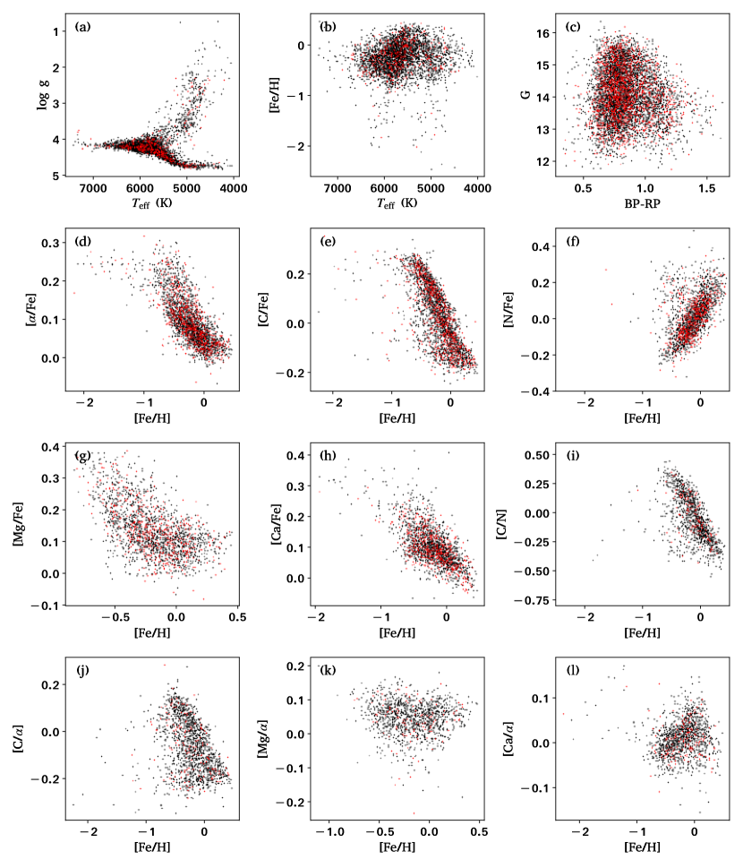
Figure 1: Distributions of the CSNet training and the testing samples in the planes of $T_{\rm eff}$–$\log g$, $T_{\rm eff}$–[Fe/H], [$BP$–$RP$]–$G$, [$\rm\alpha$/Fe]–[Fe/H], [C/Fe]–[Fe/H], [N/Fe]–[Fe/H], [Mg/Fe]–[Fe/H], [Ca/Fe]–[Fe/H], [C/N]–[Fe/H], [C/$\alpha$]–[Fe/H], [Mg/$\alpha$]–[Fe/H], and [Ca/$\alpha$]–[Fe/H], from top to bottom and left to right. The black and red dots represent the training set and testing set stars, respectively. To avoid crowding, only 10 per cent of selected stars are plotted.

3 Method: The cost-sensitive ANN

Considering the nature of the photometric data from J-PLUS DR1, we have developed CSNet, a combination of a traditional ANN architecture and a novel two-dimensional cost-sensitive learning algorithm to estimate stellar parameters and chemical abundances. Training the neural network is performed by the cost-sensitive learning algorithm in order to achieve better measurement precision.

3.1 Data normalization

Input variables with the same scale are the basis for training the robust CSNet. Thus, stellar colors are standardized before entering the network by the following z-score normalization:

$${x}^{\prime}=\frac{x-\mu}{\sigma},$$ (1)

where $x$ and ${x}^{\prime}$ are the original and standardized input vectors, respectively, with the 13 stellar colors respectively, while $\mu$ and $\sigma$ are the mean and standard deviation of all the original input vectors, respectively.

3.2 The ANN

To balance the under-fitting and over-fitting during the training process, after several experiments, the appropriate architecture for the multilayered feed-forward network in this work is 13-300-200-100-1 for estimating each stellar label, consisting of three hidden layers to extract deep features from the photometry with the 13 stellar colors. The model structure is illustrated in Fig. 2.

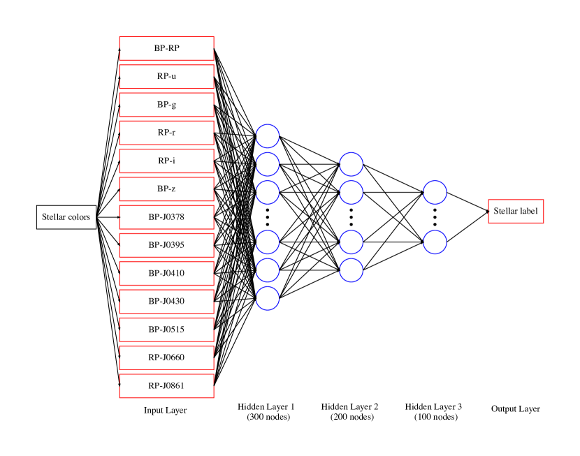
Figure 2: The ANN structure of CSNet. The structure consists of a scalable five-layered feed-forward network. The input layer imports the 13 stellar colors transformed by J-PLUS DR1 and Gaia DR2 after extinction correction as the basic features. The following three hidden layers with activation functions extract the deep non-linear features of the stellar colors. The output layer provides a stellar label with a weighted sum of the learned features in the last hidden layer.

Each node calculates a weighted sum of all its input values and produces an output value with a non-linear activation function. This process can be described as:

$$H^{l}=g(w^{(l)}X^{l}+b^{(l)}),$$ (2)

$$X^{(l+1)}=H^{l},$$ (3)

where $X^{l}$ and $H^{l}$ represent the input vector and output vector of the $l$-th layer respectively, $w$ is the weight vector, $b$ represents the bias terms and $g(\bullet)$ represents the LeakyReLU activation function with negative slope coefficient $\alpha=0.01$ in the hidden layer to solve “Dead Neuron” problems.

Then, adjustable parameters (including $w$ and $b$) of the ANN can be calculated through minimizing the following cost:

$$C(w,b)=\left\|\hat{Y}-\sum_{l=1}^{L}g_{w^{(l)},b^{(l)}}(X^{l})\right\|_{2}^{2},$$ (4)

where $\hat{Y}$ denotes the corresponding known stellar labels.

However, the over-fitting problem is more likely to occur when a large number of neurons are employed to extract deep features from the input data, which means that the accuracy of the prediction in the testing set decreases as the performance of the model in the training set improves. $L_{2}$ regularization, Dropout layers and Batch Normalization layers are all effective to mitigate this problem. In this work, a $L_{2}$ regularized term is added to the cost function above as follows:

$$C(w,b)=\left\|\hat{Y}-\sum_{l=1}^{L}g_{w^{(l)},b^{(l)}}(X^{l})\right\|_{2}^{2}+\lambda\left\|w\right\|_{2}^{2},$$ (5)

where $\lambda\in(0,1)$ is the trade-off coefficient between the residual error and the regularized term.

The back-propagation learning algorithm with adaptive moment estimation (ADAM) is utilized to minimize the cost function Eq. (5) effectively. Let $\theta=(w,b)$ be parameters of the model. Then, the change of parameter $\theta$ becomes:

$$\Delta\theta(t)=-\frac{\eta}{2}\nabla_{\theta}C(\theta(t-1))+\alpha\Delta\theta(t-1),$$ (6)

where $\eta$ is the step size, $t$ is the number of current iterations, and $\alpha\in[0,1]$ is the decay rate of the previous weight change.

The process of obtaining the resulting parameters $\theta$ can be described as follows (see Kingma & Ba 2014):

Initialize: $\eta_{t}=\frac{\eta}{\sqrt{t}}$ as the step size, $\beta_{1},\beta_{2}\in(0,1)$ as the decay rates for the moment estimate, $\epsilon>0$, $C(\theta(t))$ as a convex differentiable cost function, $\theta_{0}$ as an initial parameter vector, $m_{0}$ and $v_{0}$ as an initial 1st and 2nd moment moment vector, respectively, and $t=0$ as the initial time step.

while: $\theta(t)$ not converged do:

$t=t+1$

$g_{t}=\nabla_{\theta}C(\theta(t-1))$

$m_{t}=\beta_{1}m_{t-1}+(1-\beta_{1})g_{t}$

$v_{t}=\beta_{2}v_{t-1}+(1-\beta_{1})g_{t}^{2}$

$\hat{m_{t}}=m_{t}/(1-\beta_{1}^{t})$

$\hat{v_{t}}=v_{t}/(1-\beta_{2}^{t})$

$\theta(t)=\theta(t-1)-\eta_{t}\hat{m_{t}}/(\sqrt{\hat{v_{t}}}+\epsilon)$

end

return $\theta(t)$

Next, a mapping from the input stellar colors to the output stellar labels is established with definite parameters $\theta=(w,b)$.

3.3 Modifications of the ANN

When the training set exhibits an unbalanced distribution in the population, the most frequent cases dominate the predicted values. Namely, the predictions will have a systematic trend towards the coverage of the greatest number of target values. Oommen et al. (2011) showed that techniques reducing the sampling bias in the target value space could improve the prediction precision for regression tasks.

In this paper, we modify the cost function in the ANN which takes the rare target values into account. Given an input dataset $X$ with continuous numeric label pairs $(Y_{1},Y_{2})$, a frequency distribution histogram is generated with $M*N$ bins in $Y_{1}$–$Y_{2}$ space, where $Y_{1}$ represents one of the given stellar labels and $Y_{2}$ represents the [Fe/H] value. Next, different costs are computed for samples in different bins of the histogram with the following rule:

$$c(x_{i})=\left(\frac{f_{n}(y_{1}^{i},y_{2}^{i})}{max(f_{n}(Y_{1}.Y_{2}))}\right)^{-\gamma},$$ (7)

where $x_{i}\in X$ is a sample, $f_{n}(\bullet)$ is a function to calculate the frequency of samples in a bin which includes $(y_{1}^{i},y_{2}^{i})$ in the histogram, and $\gamma>0$ controls the difference degree of the cost among different bins.

Then, the cost function of ANN in Eq. (5) is changed to:

$$C(w,b)=c(X)\left\|\hat{Y}-\sum_{l=1}^{L}g_{w^{(l)},b^{(l)}}(X^{l})\right\|_{2}^{2}+\lambda\left\|w\right\|_{2}^{2},$$ (8)

This favors labels of the minority cases with higher expected error costs.

4 Results

To demonstrate the accuracy and reliability of the results from CSNet, we perform extensive experiments examining the estimated stellar labels from different aspects. After introducing the experimental setting, we train and test CSNet with the constructed data set (see Section 2.3), and compare the measurements on the stars in common with other precision survey catalogs. Then we apply this model to 4,387,568 stars (MAGABDUALOBJ_CLASS_STAR $\geq$ 0.6) selected by cross-matching J-PLUS DR1 with Gaia DR2.

4.1 Experimental setting

The experiments are performed with Keras 2.1.4, Tensorflow 1.5.0, CUDA 9, and cuDNN 7. ADAM is used as the optimizer because of its good robustness to the initial learning rate. Before training CSNet, there are several hyper-parameters that have been set manually: $s$ is the batch size of the training samples, $epoch$ defines the training iterations, $\eta$ is the learning rate, $M*N$ is the number of bins in the training set frequency distribution histogram, $\gamma$ is the exponent of the weight assignment function Eq. (7), $\lambda$ is the penalty coefficient of the cost function Eq. (8), and the parameters ($\beta_{1},\beta_{2},\epsilon$) for ADAM. Large $s$ occupying the GPU memory speeds the convergence, small $\eta$ consuming more time helps find the optimal value, proper $\gamma$ ensures similar distribution between the training and testing set, $\lambda$ is positively associated with the typical value of the loss function, and other hyper-parameters ($\beta_{1},\beta_{2},\epsilon$) in ADAM can use its default values. From experimentation, we found that reasonable default settings for the stellar label determination are $s=2000$, $epoch=5000$, $\eta=10^{-4}$, $\gamma=0.5$, $\lambda=5*10^{-5}$, $\beta_{1}=0.9$, $\beta_{2}=0.999$, and $\epsilon=10^{-8}$. According to the range of the expected stellar labels, recommended bins (M*N) are ($20*1$), ($20*1$), ($20*1$), ($20*60$), ($28*60$), ($35*50$), ($20*40$) and ($25*60$) for $T_{\rm eff}$, $\log g$, [Fe/H], [$\alpha$/Fe], [C/Fe], [N/Fe], [Mg/Fe], and [Ca/Fe], respectively.

4.2 Performance

We restrict the application of CSNet only to stars within the same [$BP$–$RP$] coverage as the training set. Furthermore, only stellar label estimates located in the same range with the training set (see Table 2) are considered to be reliable, as we are cautious to extrapolate, a well-known limitation of ANN-based approaches. We evaluated the performance of these labels on the training, testing, and validation samples.

4.2.1 Parameter determination on the training and the testing sets

To assess the accuracy of stellar labels derived from our model, we first compare the predictions from the model and their corresponding LAMOST labels in both the training and the testing sets.

For the stellar parameters ($T_{\rm eff}$, $\log g$, and [Fe/H]), Fig. 3 plots distributions of the CSNet results in the plane of $T_{\rm eff}$–$\log g$ (panel (a)) and residuals for dwarfs and giants as a function of effective temperature (panels (b), (c), and (e)), surface gravity (panel (d)) and metallicity (panel (f)). Giant stars ($BP-RP>0.95$ and $M_{G}<3.9$) and dwarf stars ($BP-RP\leq 0.95$ or $M_{G}\geq 3.9$) are distinguished in the color-magnitude diagram. The top two panels show that giants and dwarfs are also clearly distinguished in the plane of $T_{\rm eff}$–$\log g$. Errors of the predicted stellar labels are evaluated by the mean deviation (“bias”) and $1\sigma$ uncertainties, which are estimated using Gaussian fits. There is no significant bias in the training and the testing sets between the CSNet results and the LAMOST values, even in regions with small numbers of training stars, demonstrating that the trained model is robust to the small sample field and avoids over-fitting. The uncertainties of the residuals are $\delta\,T_{\rm eff}\sim$ 55 K, $\delta\log g\sim 0.15$ dex, and $\delta$ [Fe/H] $\sim$ 0.07 dex, respectively.

Similarly, for the elemental abundances, Fig. 4 indicates that the results are commensurate with the reference values in both the training and the testing sets. The uncertainties of the residuals are $\delta\,$[$\alpha$/Fe] = 0.03 dex, $\delta$ [C/Fe] = 0.04 dex, $\delta$ [N/Fe] = 0.08 dex, $\delta$ [Mg/Fe] = 0.05 dex, and $\delta$ [Ca/Fe] = 0.05 dex, respectively. The low levels of bias and uncertainty between the CSNet predictions and LAMOST DD-Payne values suggest that the trained model performs well on abundance determinations over the validity range.

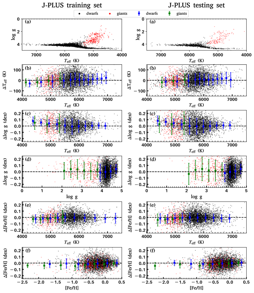
Figure 3: Training set (left) and testing set (right) for $T_{\rm eff}$, $\log g$, and [Fe/H] for the CSNet results. The black and red dots represent dwarfs and giants, respectively. Error bars, colored by blue and green for dwarfs and giants respectively, denote the mean value “bias” and 1 $\sigma$ uncertainty of the residuals estimated using Gaussian fits.

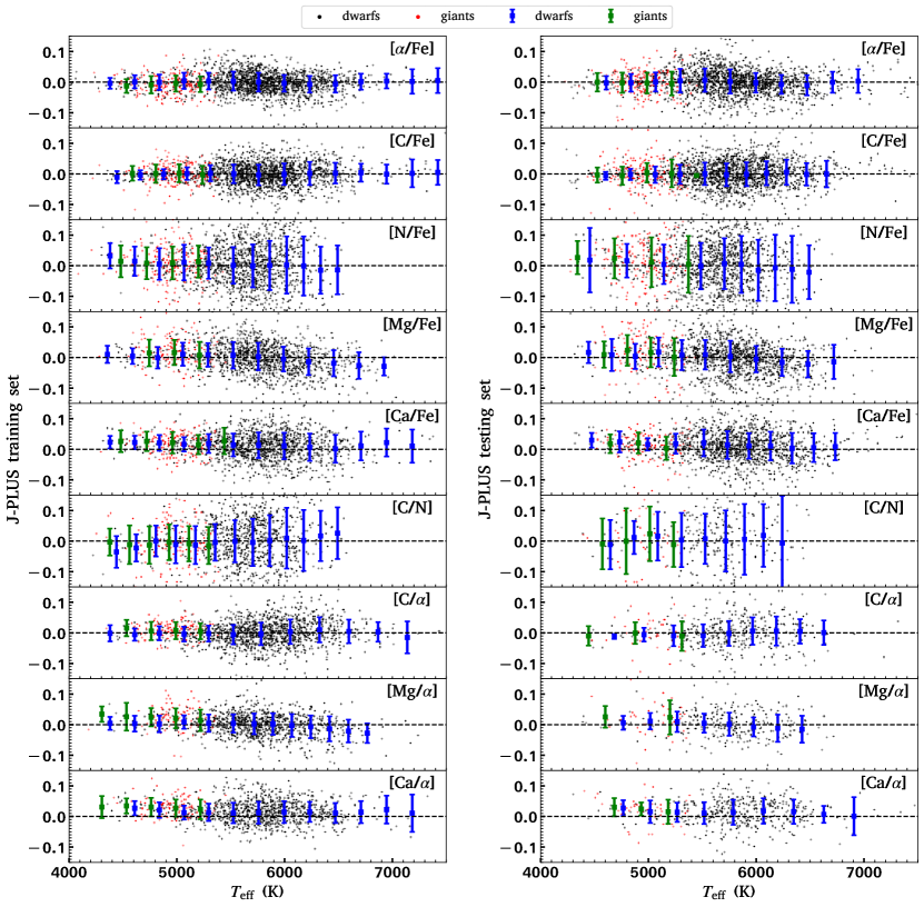
Figure 4: Similar to Fig. 3, but here we show residuals for the CSNet elemental abundances as a function of effective temperature.

4.2.2 Comparisons with other surveys

To examine the reliability of the CSNet results, we select stars in common between the J-PLUS DR1 and other reference catalogs including precise stellar parameters and elemental abundances derived from their available spectra.

1. APOGEE–Payne: The Apache Point Observatory for Galactic Evolution Experiment (APOGEE; Majewski et al. 2017) is a high-resolution ($R\sim 22,500$), high signal-to-noise ratio ($\rm S/N>100$), near-infrared (1.51–1.70 $\mu$m) spectroscopic survey. Ting et al. (2019) provide accurate stellar parameters and abundances derived from the APOGEE DR14 spectra with the neural-network based method The Payne. We cross-match the J-PLUS DR1 stars with the APOGEE–Payne catalog, finding 7,703 stars in common.

2. APOGEE–ASPCAP: APOGEE Stellar Parameters and Chemical Abundances Pipeline (ASPCAP; García Pérez et al. 2016) produces a catalog of stellar labels for the Data Release 15 (DR15) of APOGEE with all quantities for each combined spectrum. We cross-match the J-PLUS DR1 with the APOGEE–ASPCAP catalog for stars with S/N higher than 100, and obtain 10,688 stars in common.

3. GALAH–Cannon: The Galactic Archaeology with HERMES (GALAH; De Silva et al. 2015) is a high-resolution ($R\sim 28,000$) spectroscopic survey using the Anglo-Australian Telescope over a 2 degree field of view. The Data Release 2 (DR2) of GALAH contains the catalog of stellar parameters and abundances determined by the data-driven algorithm The Cannon (Ness et al. 2015). We cross-match the J-PLUS DR1 with the GALAH–Cannon catalog and obtain 252 stars in common.

Fig. 5 shows the comparisons of $T_{\rm eff}$, $\log g$, and [Fe/H] between our results and the above three reference catalogs. Overall, our results are in good agreement with the values from these catalogs. We do not expect a perfect match, considering that the reference LAMOST DR5 catalog used for training has differences with respect to these three catalogs. The APOGEE–Payne $T_{\rm eff}$ values are consistent with ours for both giant and dwarf stars, except for dwarfs with $T_{\rm eff}$ lower than 4800 K, where there is an obvious systematic trend — the APOGEE–Payne values are higher than ours, and the bias reaches about 100–220 K. Another noticeable difference is for the giant stars with $T_{\rm eff}$ lower than 4300 K, as the APOGEE–Payne $\log g$ values are lower than ours, and the bias reaches 0.2–0.3 dex. The difference between [Fe/H] from our result and that from the APOGEE–Payne shows weak systemic trends for dwarf stars with $T_{\rm eff}$ lower than 4800 K, and the bias reaches 0.10–0.22 dex. Similar to the comparisons between the APOGEE–Payne values and ours, APOGEE–ASPCAP and GALAH–Cannon exhibit good consistency with the results from our method, except that both sets of results also show systematic deviations in $T_{\rm eff}$ and [Fe/H] for dwarf stars ($T_{\rm eff}<4800$ K), and $\log g$ for giant stars ($T_{\rm eff}<4300$ K). These differences in $T_{\rm eff}$, $\log g$, and [Fe/H] mainly reflect the systematic differences in our training set, LAMOST DR5, and the reference catalogs. Direct comparisons of the LAMOST DR5, APOGEE–Payne, APOGEE–ASPCAP, and GALAH–Cannon stellar parameters for stars in common are presented in the Appendix (Fig. 23). It shows consistent patterns with those presented in Fig. 5, demonstrating that CSNet has merely inherited the systematic errors from the training sets.

Fig. 6 shows the comparisons of elemental abundances between our estimates and that of APOGEE–Payne, APOGEE–ASPCAP and GALAH–Cannon. A close inspection suggests that there are systematic offsets and trends for [Mg/Fe] and [Ca/Fe] compared to the results from of APOGEE–Payne and APOGEE–ASPCAP. However, our [Mg/Fe] estimates are more consistent with that of GALAH–Cannon. This is because the [Mg/Fe] in the LAMOST–DD-Payne catalog, which is our training set, is derived using the GALAH–Cannon values as a reference (see Section 2.2). Systematic deviations of the other elemental abundances (e.g., [$\alpha/$Fe], [C/Fe], [N/Fe], and [Ca/Fe]) are inherited from the differences among the reference catalogs, as consistent difference patterns exist in the training sets shown in the Appendix (Fig. 24).

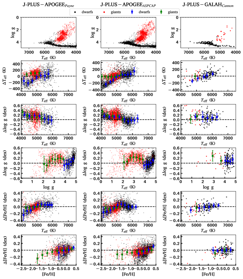
Figure 5: Similar to Fig. 3, but for stars in common between the CSNet results and the reference catalogs.

Figure 6: Similar to Fig. 4, but for stars in common between the CSNet results and the reference catalogs.

4.3 The J-PLUS DR1 catalog of stellar parameters and chemical abundances

We select 4,387,568 stars (MAGABDUALOBJ_CLASS_STAR $\geq$ 0.6) by cross-matching J-PLUS DR1 with Gaia DR2, and determine their stellar parameters and chemical abundances using CSNet. The catalog is publicly available . A description of the J-PLUS CSNet stellar parameters and chemical abundances catalog is provided in Table 2.

Considering the photometric quality of J-PLUS DR1 and the limitations of CSNet, we recommend stellar labels for 2,343,597 stars with FLAGS $=$ 0 in all 12 J-PLUS filters and $0.063<BP-RP<1.786$. As discussed in Section 4.2.2, $T_{\rm eff}$ for dwarf stars ($T_{\rm eff}<4800$ K), and $\log g$ for giant stars ($T_{\rm eff}<4500$ K) in our results should be used with caution, because they show non-negligible systematic errors related to the $T_{\rm eff}$ values. To avoid large label uncertainties caused by photometric errors, particularly for elemental abundances, we further select 0.61 million stars with $G<18$ and magnitude errors in the 12 J-PLUS filters less than 0.1 mag, including 0.57 million dwarfs and 44,686 giants. Note that the giants and dwarfs are distinguished in the color-magnitude diagram ($BP-RP>0.95$ and $M_{G}<3.9$ for giants; $BP-RP\leq 0.95$ or $M_{G}\geq 3.9$ for dwarfs). Fig. 7 and 8 show the stellar density distributions in the planes of $T_{\rm eff}$–$\log g$, $T_{\rm eff}$–[Fe/H], ($BP-RP$)–$G$, and different CSNet abundances with respect to [Fe/H] for the 0.57 million dwarfs and 44,686 giants, respectively. Their distributions in the $T_{\rm eff}$–$\log g$ diagrams are consistent with those in the color-magnitude diagrams. The abundance trends are encouraging, and are consistent with literature results from LAMOST DD–Payne (Fig. 25 and Fig. 26). Fig. 9 and 10 show distributions of the number density and different CSNet abundances in the R–Z plane for the same sets of dwarfs and giants, respectively. Similarly, the abundance trends perform as expected. For example, values of [Fe/H] decrease and values of [Mg/Fe] and [C/N] increase with increasing distance from the Galactic plane. Detailed scientific investigations of the catalog, such as stellar populations, Galactic components and gradients based on these abundance results, will be presented in the future.

Table 3: Description for the J-PLUS CSNet stellar parameters and chemical abundances catalog.¹

Col.	Field	Description
1	specid	J-PLUS source id
2	gl	Galactic longitude from the J-PLUS DR1 catalog (deg)
3	gb	Galactic latitude from the J-PLUS DR1 catalog (deg)
4	ra	Right ascension from the J-PLUS DR1 catalog (J2000; deg)
5	dec	Declination from the J-PLUS DR1 catalog (J2000; deg)
6	MAG_APER6	Photometry in 12 filters from the re-calibrated J-PLUS DR1 catalog
7	ERR_APER6	Uncertainty in MAG_APER6 (mag)
8	FLAGS	Inherited from SExtractor’s FLAGS parameter
9	PHOT_BP_MEAN_MAG	$BP$-band photometry from Gaia DR2
10	PHOT_RP_MEAN_MAG	$RP$-band photometry from Gaia DR2
11	PHOT_G_MEAN_MAG	$G$-band photometry from Gaia DR2
12	$E(B-V)$	Interstellar extinction from the Schlegel et al. (1998) dust-reddening map
7	$T_{\rm eff}$	Effective temperature (K)
8	$T_{\rm eff}$_flag1	A quality flag for $T_{\rm eff}$
9	$\log g$	Surface gravity
10	$\log g$_flag1	A quality flag for $\log g$
11	[Fe/H]	Iron to hydrogen abundance ratio
12	[Fe/H]_flag1	A quality flag for [Fe/H]
13	[$\alpha$/Fe]	$\alpha$-element to iron abundance ratio
14	[$\alpha$/Fe]_flag1	A quality flag for [$\alpha$/Fe]
15	[C/Fe]	Carbon to iron abundance ratio
16	[C/Fe]_flag1	A quality flag for [C/Fe]
17	[N/Fe]	Nitrogen to iron abundance ratio
18	[N/Fe]_flag1	A quality flag for [N/Fe]
19	[Mg/Fe]	Magnesium to iron abundance ratio
20	[Mg/Fe]_flag1	A quality flag for [Mg/Fe]
21	[Ca/Fe]	Calcium to iron abundance ratio
22	[Ca/Fe]_flag1	A quality flag for [Ca/Fe]

• Flag = 0 (reliable) means that the object’s $BP-RP$ color is within the effective $BP-RP$ range given in Table 2, flag = 1 otherwise.

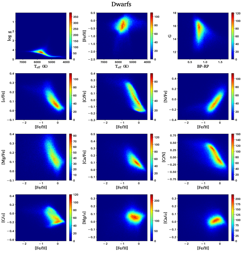
Figure 7: Density distributions of selected J-PLUS DR1 dwarf stars in the planes of $T_{\rm eff}$–$\log g$, $T_{\rm eff}$–[Fe/H], ($BP-RP$)–$G$, and different CSNet abundances with respect to [Fe/H], all color-coded by stellar number density. Only stars with reliable labels by the following criteria are used: (1) FLAGS = 0; (2) $0.063<BP-RP<1.786$; (3) $G<18$; (4) err (all J-PLUS filters) ¡ 0.1 mag.

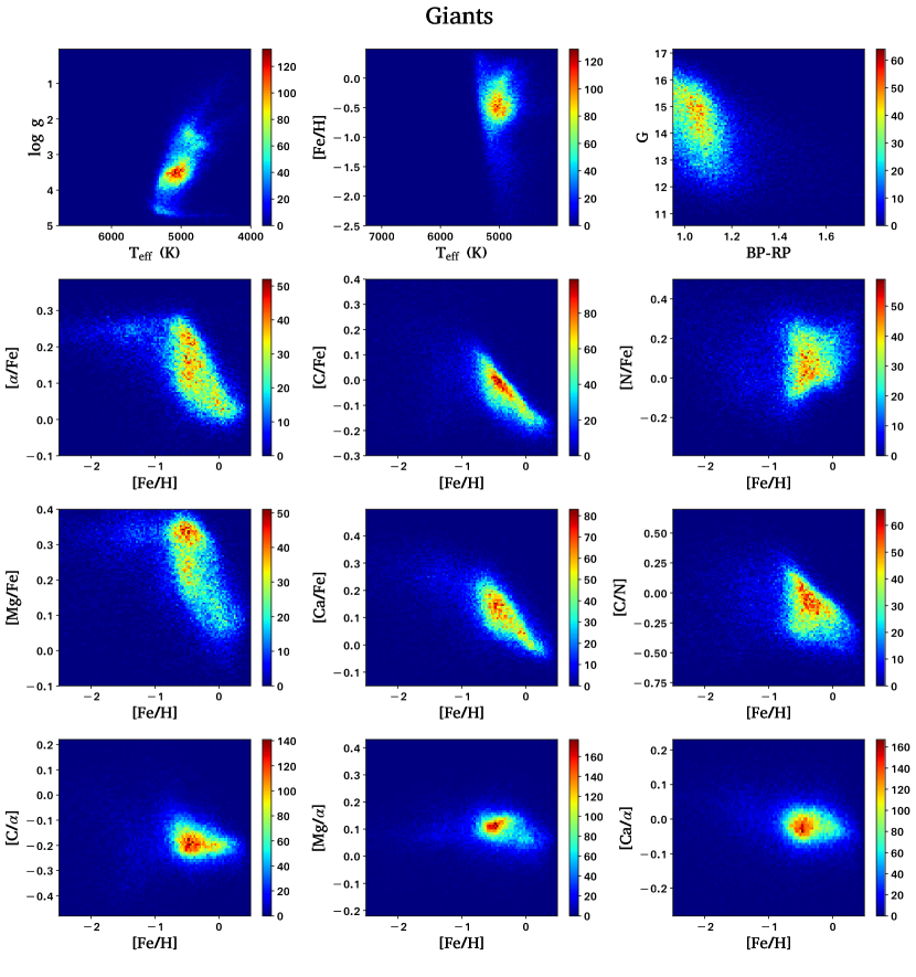
Figure 8: Similar to Fig. 7, but for selected J-PLUS DR1 giant stars.

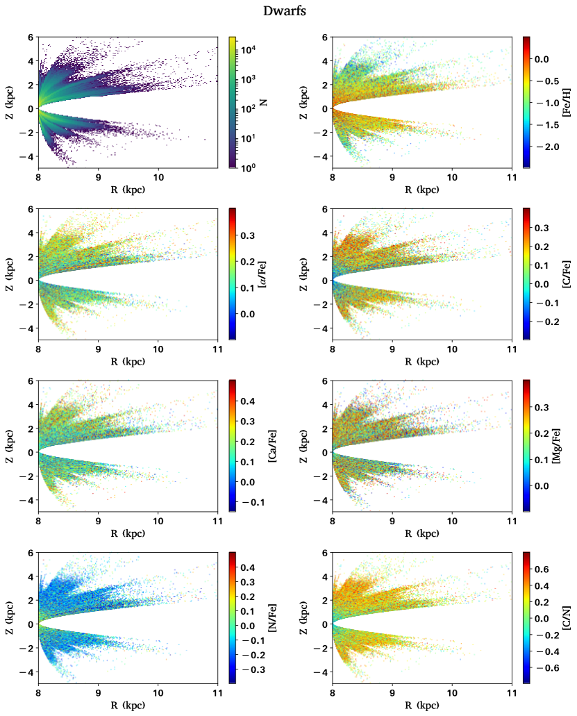
Figure 9: Distributions of number density and different CSNet abundances in the plane of R–Z for selected J-PLUS DR1 dwarf stars. Only stars with reliable labels by the following criteria are used: (1) FLAGS = 0; (2) $0.063<BP-RP<1.786$; (3) $G<18$; (4) err (all J-PLUS filters) ¡ 0.1 mag.

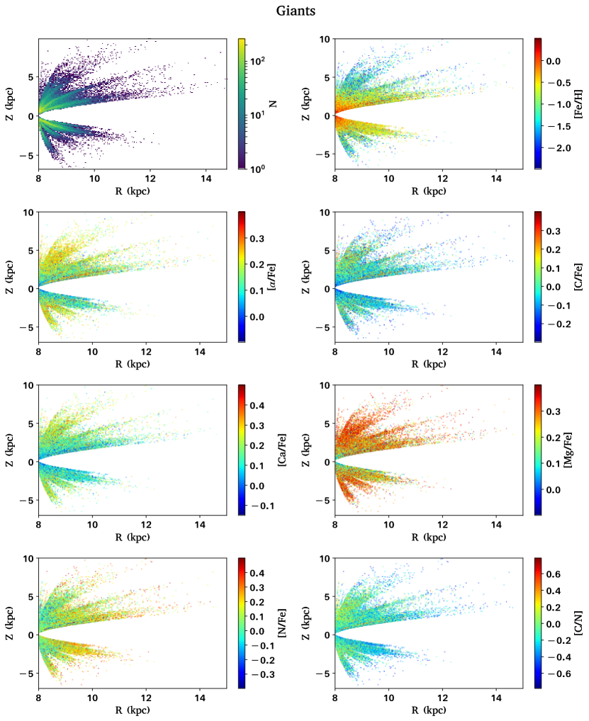
Figure 10: Similar to Fig. 9, but for selected J-PLUS DR1 giant stars.

5 Discussion

We combine the recalibrated J-PLUS DR1 and Gaia DR2 to construct 13 stellar colors. Then, the cost-sensitive neural-network based CSNet algorithm is designed and trained to map from the 13 colors to precise stellar labels. Thanks to the specially designed J-PLUS filters and Gaia BP/RP passbands, CSNet can not only determine the basic stellar atmospheric parameters (effective temperature, $T_{\rm eff}$, surface gravity, $\log g$, and metallicity, [Fe/H]), but also deliver [$\alpha$/Fe] and elemental abundances including [C/Fe], [N/Fe], [Mg/Fe], and [Ca/Fe]. This method performs well even if the training set has a sub-optimal distribution of stellar sample properties by increasing the error penalty for the rare subsets of stars. Our results show a high level of agreement with those from the testing samples. Comparisons with the APOGEE–Payne, APOGEE–ASPCAP, and GALAH–Cannon stars also show a good agreement, although some systematic discrepancies do exist, mainly caused by the systematic errors between the different surveys (see more details in Appendix B).

We also investigate the accuracy of the CSNet approach to derive the reddening, $E(B-V)$. Additional experiments show that CSNet is capable of estimating the $E(B-V)$ from stellar colors with a 1$\sigma$ uncertainty smaller than 0.02 mag. When CSNet is trained using the stellar colors without reddening correction, it achieves slightly lower accuracy for most stellar labels, suggesting that the J-PLUS filters should work well in regions of high extinction.

Deep learning networks, including CSNet, require sufficient data with known labels to train and test a reliable model, which limits the coverage of the stellar labels that can be predicted. In the future, we plan to improve our method to estimate [Fe/H] for very and extremely metal-poor stars. In addition, there are chemically peculiar stars (e.g., the carbon-enhanced metal-poor stars) with abundance ratios that lie outside the ranges we presently explore. We plan to remedy this limitation with the addition of such stars to the training/testing samples in the near future.

We point out that the J-PLUS and S-PLUS surveys are ongoing, and rapidly growing in their coverage of the Northern and Southern Hemispheres, respectively. Application of CSnet, and its planned refinements, to both of these datasets will eventually be able to provide similar results as presented in this paper for hundreds of millions of stars over much of the sky.

6 Summary

By combining photometric data from the recalibrated J-PLUS DR1, Gaia DR2, and spectroscopic labels from LAMOST, we design and train a cost-sensitive neural network, CSNet, to learn the non-linear mapping from stellar colors to their labels. Special attention is paid to the minority populations in the label space by assigning different weights according to their density distributions. Thanks to the specially designed J-PLUS narrow-band filters, CSNet can not only determine the basic stellar atmospheric parameters (effective temperature, $T_{\rm eff}$, surface gravity, $\log g$, and metallicity, [Fe/H]), but also deliver [$\alpha$/Fe] and elemental abundances including [C/Fe], [N/Fe], [Mg/Fe], and [Ca/Fe]. We have achieved precisions of $\delta\,T_{\rm eff}\sim$ 55 K, $\delta\log g\sim 0.15$ dex, and $\delta$ [Fe/H] $\sim$ 0.07 dex, respectively. The uncertainties of the abundance estimates for [$\alpha$/Fe] and the four individual elements are on the order of $\delta$  $\sim$ 0.04–0.08 dex. We compare our parameter and abundance estimates with those from other spectroscopic catalogs such as APOGEE and GALAH, finding an overall good agreement. Applying our method to J-PLUS DR1, we have obtained the aforementioned parameters for over two million stars, providing a powerful data set for chemo-dynamical analyses of the Milky Way. The catalog of the estimated parameters is publicly accessible. Our results also demonstrate the potential of well-designed and high-quality photometric data in determinations of stellar parameters as well as for individual elemental abundances.

Appendix A Correlation analyses between J-PLUS colors and stellar labels

The core idea of CSNet is to construct a mapping from J-PLUS colors to stellar labels. This leaves the question as to whether our results are from specific sensitive J-PLUS colors or just from correlations among the stellar labels themselves.

Figs. 11–16 show comparisons for [Mg/Fe], [C/Fe], and [N/Fe] between our results and LAMOST DD–Payne in the plane of [X-Fe]–[Fe/H]. The differences between the CSNet results and the LAMOST DD–Payne are very small. Figs. 17–22 show comparisons in the color-color diagrams ($BP-J0515$ – $BP-RP$ for [Mg/Fe], $BP-J0430$ – $BP-RP$ for [C/Fe], and $BP-J0378$ – $BP-RP$ for [N/Fe]). We can see that abundances of our results are all consistent with those of LAMOST DD–Payne, indicating that the training process of CSNet works as expected. At a given narrow [Fe/H] range and $BP-RP$ color, correlations between $BP-J0515$ and [Mg/Fe], $BP-J0430$ and [C/Fe], $BP-J0378$ and [N/Fe] are significant, demonstrating that CSNet measures these elemental abundances from $ab\,initio$ features, rather than drawing on astrophysical correlations among the stellar labels.

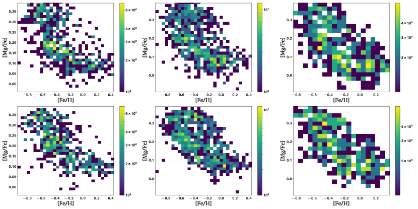
Figure 11: Stellar number density distributions in the plane of [Mg/Fe] – [Fe/H] from the LAMOST catalog (top panels) and the CSNet results (bottom panels) for the training/testing sample giant stars, all color-coded by stellar number density. Different columns are for stars of different $BP-RP$ ranges. From left to right these are [0.95, 1.05], [1.05, 1.15], and [1.15, 1.40], respectively.

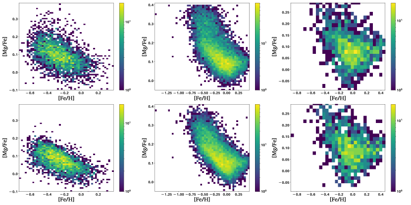
Figure 12: Similar to Fig. 11, but for the dwarf stars. The $BP-RP$ ranges are [0.25, 0.70] (left column), [0.70, 1.00] (middle column) and [1.00, 1.50] (right column), respectively.

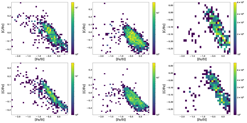
Figure 13: Stellar number density distributions in the plane of [C/Fe] – [Fe/H] from the LAMOST DD–Payne (top panels) and the CSNet results (bottom panels) for the training/testing sample giant stars, all color-coded by stellar number density. Different columns are for stars of different $BP-RP$ ranges. From left to right these are [0.95, 1.05], [1.05, 1.20], and [1.20, 1.60], respectively.

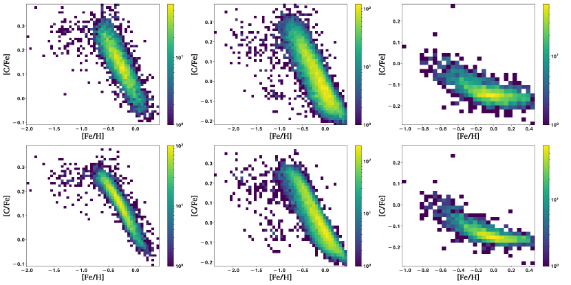
Figure 14: Similar to Fig. 13, but for the dwarf stars. The $BP-RP$ ranges are [0.25, 0.70] (left column), [0.70, 1.00] (middle column) and [1.00, 1.50] (right column), respectively.

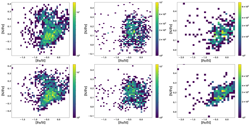
Figure 15: Stellar number density distributions in the plane of [N/Fe] – [Fe/H] from the LAMOST DD–Payne (top panels) and the CSNet results (bottom panels) for the training/testing sample giant stars, all color-coded by stellar number density. Different columns are for stars of different $BP-RP$ ranges. From left to right these are [0.95, 1.10], [1.10, 1.20], and [1.20, 1.60], respectively.

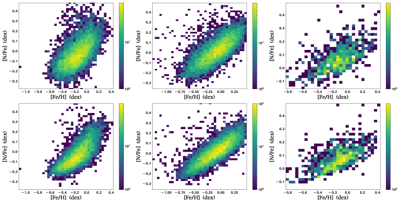
Figure 16: Similar to Fig. 15, but for the dwarf stars. The $BP-RP$ ranges are [0.50, 0.80] (left column), [0.80, 1.10] (middle column) and [1.10, 1.50] (right column), respectively.

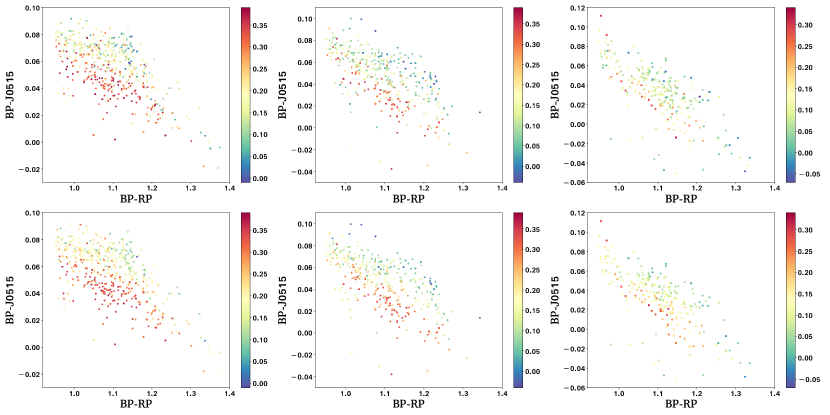
Figure 17: Distributions of [Mg/Fe] in the [$BP-RP$] – [$BP-J0515$] color-color diagram from the LAMOST DD–Payne (top panels) and the CSNet results (bottom panels) for the training/testing sample giant stars, all color-coded by [Mg/Fe]. Different columns are for stars of different [Fe/H] ranges. From left to right these are [$-$0.5, $-$0.3], [$-$0.3, $-$0.1], and [$-$0.1, 0.1], respectively.

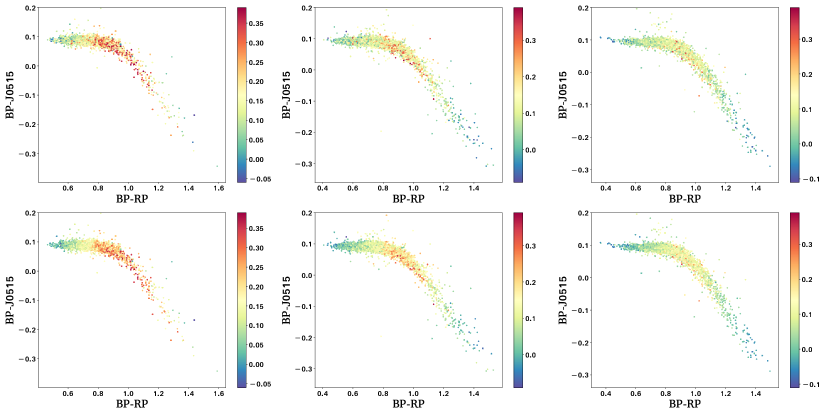
Figure 18: Similar to Fig. 17, but for the dwarf stars.

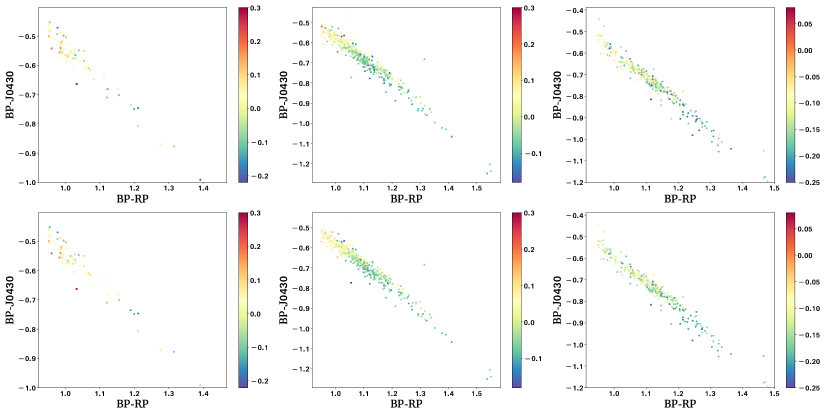
Figure 19: Distributions of [C/Fe] in the [$BP-RP$] – [$BP-J0430$] color-color diagram from the LAMOST DD–Payne (top panels) and the CSNet results (bottom panels) for the training/testing sample giant stars, all color-coded by [C/Fe]. Different columns are for stars of different [Fe/H] ranges. From left to right these are [$-$1.2, $-$0.9], [$-$0.7, $-$0.5], and [$-$0.1, 0.1], respectively.

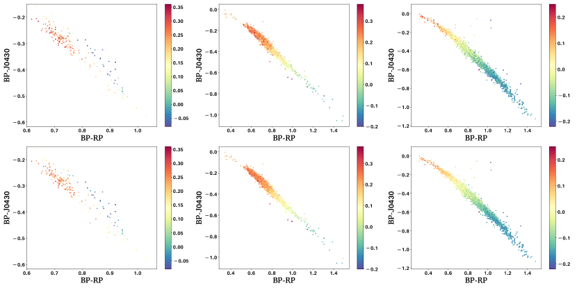
Figure 20: Similar to Fig. 19, but for the dwarf stars.

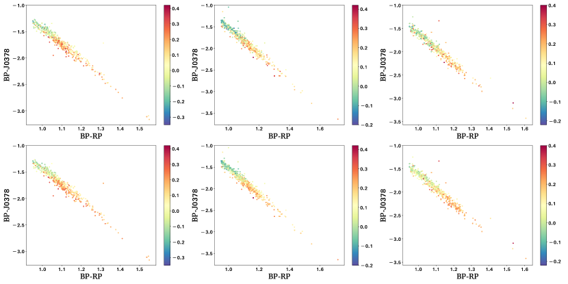
Figure 21: Distributions of [N/Fe] in the [$BP-RP$] – [$BP-J0378$] color-color diagram from the LAMOST DD–Payne (top panels) and the CSNet results (bottom panels) for the training/test giant stars, all color-coded by [N/Fe]. Different columns are for stars of different [Fe/H] ranges. From left to right these are [$-$0.7, $-$0.5], [$-$0.5, $-$0.3], and [$-$0.3, $-$0.1], respectively.

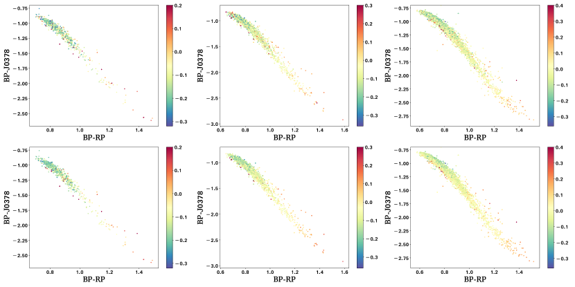
Figure 22: Similar to Fig. 21, but for the dwarf stars.

Appendix B Comparisons of LAMOST with APOGEE–Payne, APOGEE–ASPCAP and GALAH–Cannon stellar labels

We have shown in this study that systematic errors between CSNet and the validation samples are inherited from the training sets, rather than from the models themselves. Figs. 23 and Figs. 24 show comparisons of LAMOST catalogs and other surveys (APOGEE–, APOGEE–ASPCAP and GALAH–Cannon) for basic stellar atmospheric parameters and elemental abundances, respectively. Systematic discrepancies and trends for stellar labels between the LAMOST catalogs and above three surveys are found. More importantly, these patterns are consistent with those shown in the CSNet results (Figs. 5 and Figs. 6), suggesting that the systematic offsets shown in the main text are inherited from the training data.

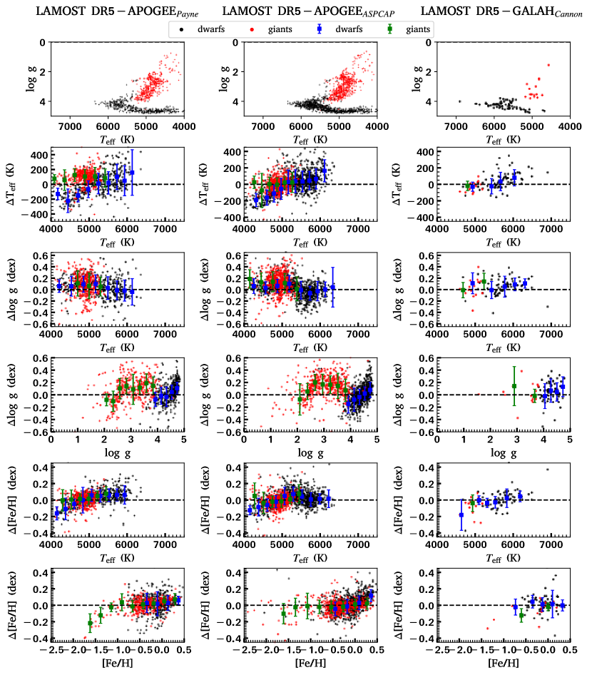
Figure 23: Comparisons for stellar atmospheric parameters including $T_{\rm eff}$, $\log g$, and [Fe/H] between the LAMOST DR5 and the APOGEE–payne (left column), APOGEE–ASPCAP (middle column), and GALAH–Cannon (right column). Only stars in commn with the LAMOST training/test samples are used. The black and red dots represent dwarfs and giants, respectively. Error bars, colored by blue and green for dwarfs and giants respectively, and indicate the mean value “bias” and 1 $\sigma$ uncertainty of the residuals estimated using Gaussian fit.

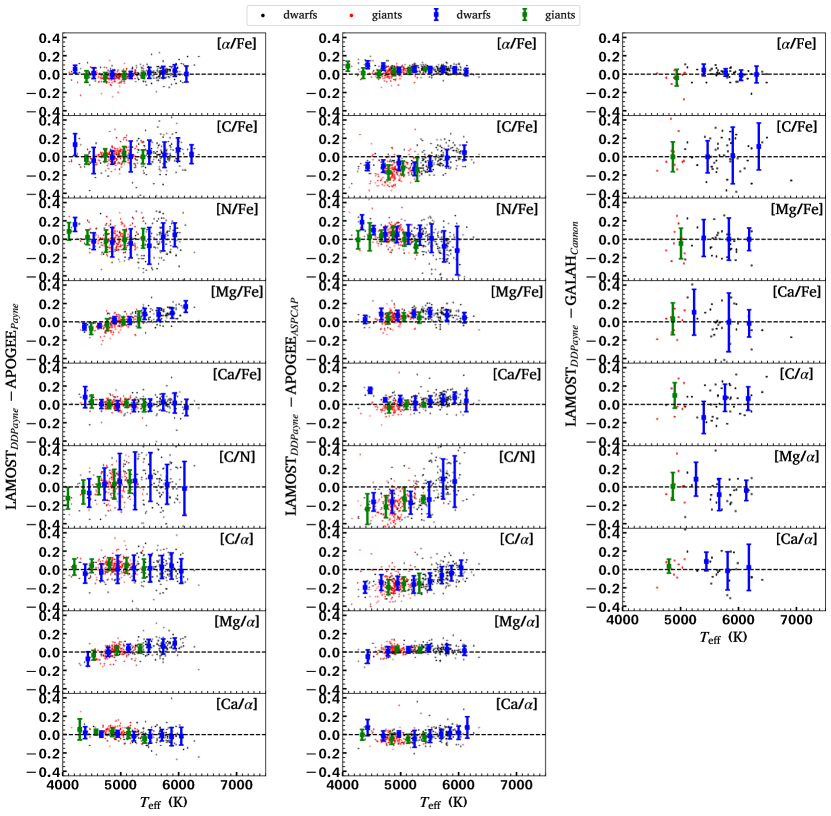
Figure 24: Similar to Fig. 23, but for the elemental abundances as a function of $T_{\rm eff}$. Note that here the LAMOST elemental abundances are from the DD–Payne.

Appendix C Stellar label distributions of LAMOST

Here we select stars in common between the J-PLUS DR1, Gaia DR2, and LAMOST DR5. For these stars we further apply the same criteria as those of Fig. 7: (1) FLAGS = 0; (2) $0.063<BP-RP<1.786$; (3) $G<18$; (4) err (all J-PLUS filters) ¡ 0.1 mag. Fig. 25 and Fig. 26 show the density distributions of the selected dwarfs and giants in the planes of $T_{\rm eff}$ – $\log g$, $T_{\rm eff}$ – [Fe/H], and ($BP-RP$) – $G$, and different elemental abundances with respect to [Fe/H], with the stellar labels from LAMOST, respectively . The results are consistent with those shown in Fig. 7 and Fig. 8.

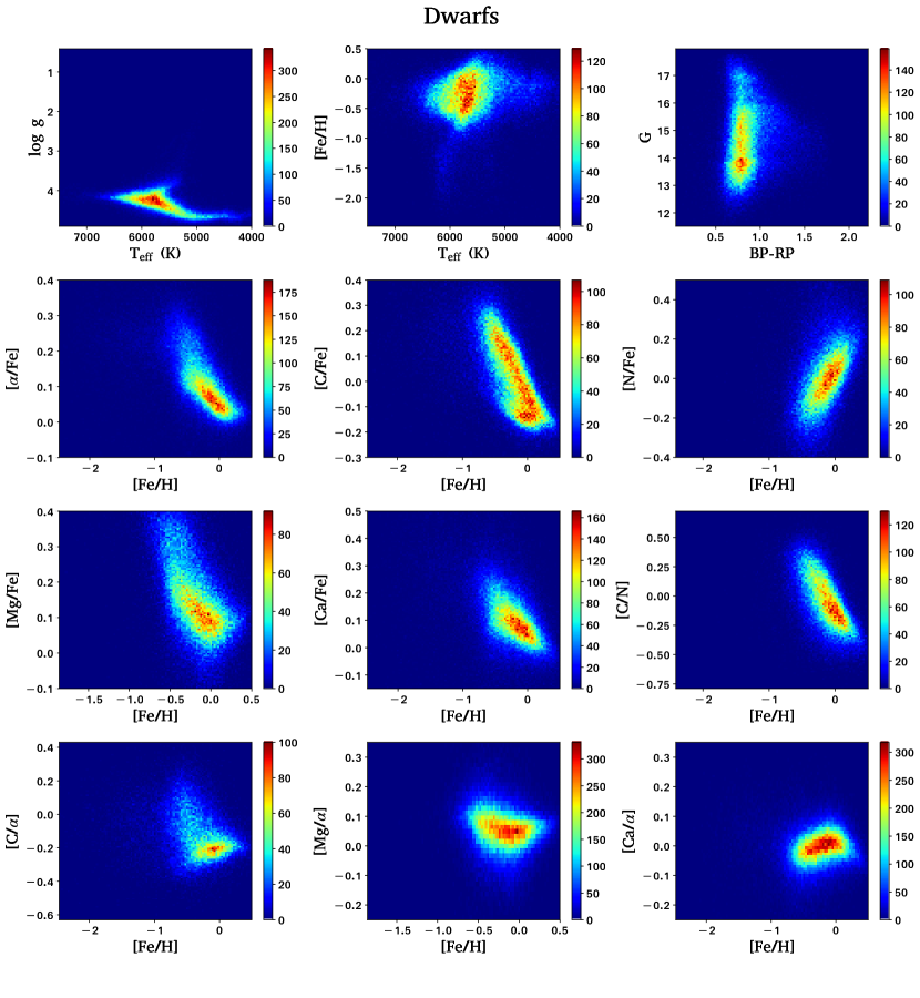
Figure 25: Density distributions of selected J-PLUS-Gaia-LAMOST dwarf stars in the planes of $T_{\rm eff}$–$\log g$, $T_{\rm eff}$–[Fe/H], ($BP-RP$)–$G$, and different elemental abundances with respect to [Fe/H], all color-coded by stellar number density. The stellar labels are from LAMOST. Only stars that satisfy the following criteria are used: (1) FLAGS = 0; (2) 0.063 ¡ BP$-$RP ¡ 1.786; (3) $G<18$; (4) err (all J-PLUS filters) ¡ 0.1 mag.

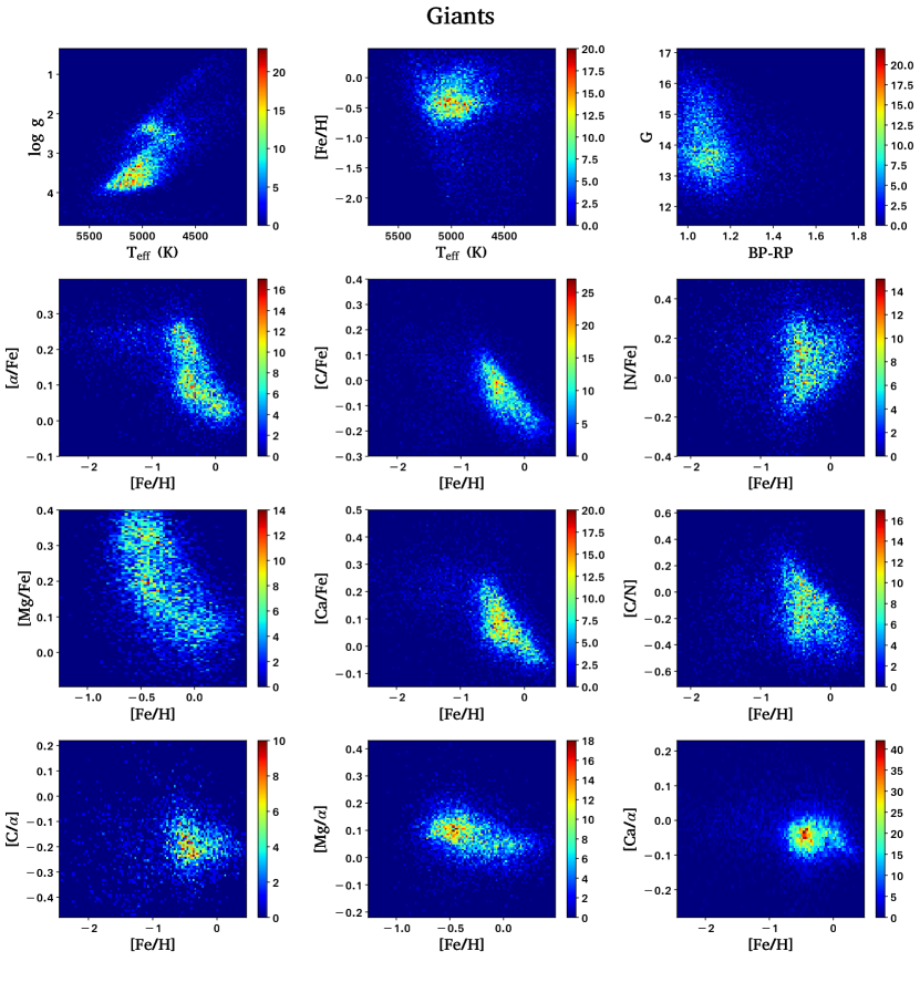
Figure 26: Similar to Fig. 25, but for giant stars.