MMO: Meta Multi-Objectivization for Software Configuration Tuning

Abstract

Software configuration tuning is essential for optimizing a given performance objective (e.g., minimizing latency). Yet, due to the software’s intrinsically complex configuration landscape and expensive measurement, there has been a rather mild success, particularly in preventing the search from being trapped in local optima. To address this issue, in this paper we take a different perspective. Instead of focusing on improving the optimizer, we work on the level of optimization model and propose a meta multi-objectivization (MMO) model that considers an auxiliary performance objective (e.g., throughput in addition to latency). What makes this model unique is that we do not optimize the auxiliary performance objective, but rather use it to make similarly-performing while different configurations less comparable (i.e. Pareto nondominated to each other), thus preventing the search from being trapped in local optima. Importantly through a new normalization method we show how to effectively use the MMO model without worrying about its weight — the only yet highly sensitive parameter that can affect its effectiveness. Experiments on 22 cases from 11 real-world software systems/environments confirm that our MMO model with the new normalization performs better than its state-of-the-art single-objective counterparts on 82% cases while achieving up to $2.09\times$ speedup. For 67% of the cases, the new normalization also enables the MMO model to outperform the instance when using it with the normalization used in our prior FSE work under pre-tuned best weights, saving a great amount of resources which would be otherwise necessary to find a good weight. We also demonstrate that the MMO model with the new normalization can consolidate Flash, a recent model-based tuning tool, on 68% of the cases with $1.22\times$ speedup in general.

1 Introduction

Many software systems are highly configurable, such that the configuration options, e.g., the splitters in Apache Storm, can be flexibly adjusted for performance, including database systems, machine learning systems, and cloud systems, to name a few. However, a daunting number of configuration options will inevitably introduce a high risk of inappropriate or even poor software configurations set by software engineers. It has been reported that 59% of the software performance issues worldwide are related to ill-suited configuration rather than code [36]. In 2017-2018, configuration-related performance issues costed at least 400,000 USD per hour for 50% of the software companies.

Indeed, adjusting the configurations will affect the outcomes of different performance attributes, such as latency, throughput, and CPU load [69, 25, 60, 24, 21, 23]. However, there are many cases wherein only the optimization of a single performance attribute is of interest, whose minimization/maximization serves as a sole performance objective in consideration. For example, in the finance sector, a millisecond decrease in the trade delay may boost a high-speed firm’s earnings by about 100 million USD per year [79]. Another example is related to the machine learning systems deployed by large organizations (e.g., GPT-3 [13]), or those in the health care domain [2], where the concern is mainly on the accuracy, while caring little about the overhead/resource incurred for training. This has been well-echoed from the literature on software configuration tuning, in the majority of which only a single performance attribute is considered at a time [7, 87, 61, 83, 52, 6, 51, 50].

Despite only a single performance attribute being of concern, such an optimization scenario is not easy to deal with for any optimizer that tunes the software configuration. This is because

1. The configurable systems involve a daunting number of configuration options with complex interactions, rendering a black-box to the software engineers [85, 17, 19, 20, 18, 22].

2. The measurement of each configuration through running the software system is often expensive [43], hence exhaustively exploring every configuration is unrealistic.

3. There is generally a high degree of sparsity in the configurable software systems [60], i.e., similar configurations can also have radically different performance.

The last characteristic poses a particular challenge to the automatic software configuration tuning in finding the optimal configuration (performance), because firstly different configurations may achieve locally good, but globally inadequate performance (e.g., local optima); and secondly, the landscape of a (local) optimum’s neighborhood can be steep and rugged — if the tuning is trapped in a local optimum, it may be hard to escape from it as their neighboring configurations often perform significantly worse than it. As an example, Figure 1 shows the projected configuration landscape for Apache Storm (2 out of 6 configuration options), where it can be clearly seen that even with this simplified version, the landscape is rather rugged and contains steep “local optimum traps”, resulting in significant difficulty in the tuning.

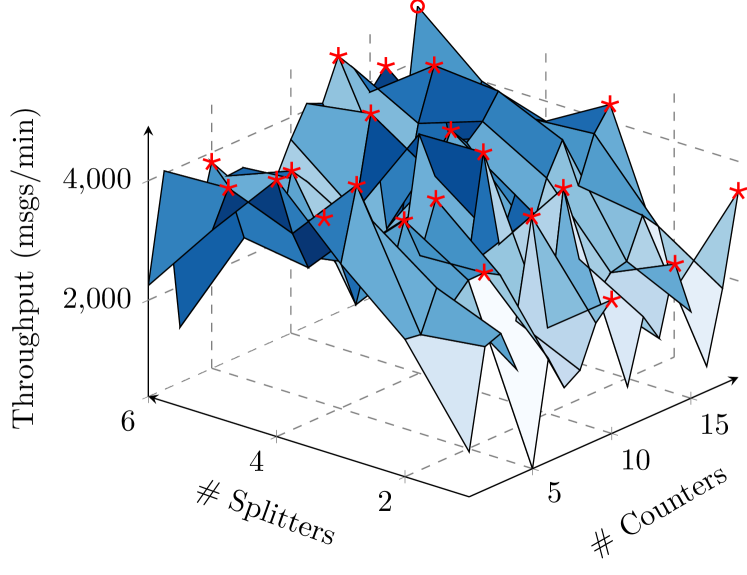
Figure 1: A projected landscape of the performance objective Throughput with respect to configuration options Splitters and Counters for Storm under the WordCount benchmark.  is the global optimum and  denotes the local optima of throughput that an optimizer needs to escape from.

In light of the above challenges, a number of optimizers from the Search-Based Software Engineering (SBSE) paradigm have been presented, such as random search [7, 87, 61], hill climbing [83, 52], genetic algorithm [6, 69, 67, 73], and simulated annealing [34, 35]. To seek the global optimum (best performance of the concerned performance attribute) while avoiding being trapped in local optima, such methods focus on the “internal” components of the optimizer. They work on designing novel search operators (i.e., the way to change the configuration structure, for example, increasing the neighbourhood size of randomly mutated configurations [61]), or developing various search strategies (i.e., the way to balance exploration and exploitation, for example, restarting the search in hill climbing [83]). However, a common limitation of such single-objective optimizers is that the goal to find the global optimum is “less oriented” as there is no clear “incentive” to encourage them to traverse the wide search space and locating many local optima as possible, thus finding the best one in a resource-efficient manner.

To better mitigate the local optima, in this paper and our prior FSE’21 work [26] (we call it FSE work thereafter), we tackle this software configuration tuning problem from a different perspective. In contrast to the effort made by the existing works on the development of the optimizer, we work on the optimization model, i.e., the “external” part of an optimizer. This is achieved by proposing a meta multi-objectivization (MMO) model for this single-objective problem, to help the search avoid being trapped in local optima and progressively explore the entire objective space.

In a nutshell, MMO seeks to optimize two meta-objectives, each of which has two components. The first component of both meta-objectives is the target performance objective (e.g., latency), thereby only those configurations that perform well on the target objective being in favor. The second component, which is related to the other given auxiliary performance objective (e.g., throughput), is a completely conflicting term for the two meta-objectives. The reason for this design is that we hope to keep the target performance objective as a primary term in the model to preserve the tendency towards its optimality, but at the same time, we want the configurations with different values on the auxiliary performance objective to be incomparable. We are not interested in minimizing/maximizing the auxiliary performance objective since we do not know which value of it can lead to the best result on the target performance objective, but we wish to keep a good amount of configurations with diverse values of the auxiliary performance objective in the search, thus not being trapped in local optima (we will elaborate this in Section 3). The contributions from both this work and the FSE work are:

• Unlike existing work for the software configuration tuning which puts efforts on the “internal part” of the optimization (i.e., improving the search operators of various optimizers), we work on the “external part” — multi-objectivizing this single-objective optimization scenario.

• We present a meta multi-objectivization model, MMO, as opposed to the existing multi-objectivization model considered in other SBSE scenarios which directly optimizes the target and auxiliary objectives simultaneously (referred to as plain multi-objectivization or PMO). We show, analytically and experimentally, why MMO is more suitable than PMO for software configuration tuning.

However, MMO requires a weight parameter to aggregate the target objective component and the auxiliary objective component. It is a critical parameter to balance searching for a good target performance objective value and maintaining diverse auxiliary performance objective values, requiring fine-tune from the software engineers for every configurable software/environment, as done in our FSE work [26]. This, if done inappropriately, could lead to poor outcomes, as we will show in Section 3.5. Yet, since measurement of configurations is often expensive, finding the best weight in a case-by-case manner is not always realistic, which is a major threat to the applicability of the MMO model.

Therefore, in this paper, we also tackle this unwelcome issue. We show why the weight can be a highly sensitive parameter in the MMO model and propose a way to make the model parameter-free while without compromising the result. This is achieved by presenting a new normalization method, which is simple, but works very well — it leads to results that are even better than those of the FSE work under its best-tuned weight [26] for the majority of the problems. To sum up, the unique contributions of this paper are:

• A detailed analysis, with evidence, that explains what makes the weight being a highly sensitive parameter for the MMO model in the FSE work.

• Drawing on insights from the analysis, we design a new normalization method, as part of the MMO model, allowing for capturing the bounds of both performance objectives adaptively. This enables us to keep the strengths and characteristics of the MMO model while removing the weight (i.e., setting $w=1$ for all cases).

• An extensive evaluation that expands to 11 systems/environments that are of very different domains. Since a system comes with two performance objectives, each of these is used in turn as the target performance objective, leading to 22 cases. Under these cases, we compare MMO model using the new normalization with the PMO model and four single-objective counterparts, as well as with the MMO model using the normalization from the FSE work.

• An investigation on whether our MMO model with the new normalization can consolidate Flash [60], which is a recently proposed model-based tuning method for general software configuration tuning.

Our experiment results are encouraging: we show that the MMO model with the new normalization achieves better results over the best single-objective counterpart and PMO (on 18 and 20 out of 22 cases wherein 14 and 15 of them are considerably better, respectively), while being much more resource-efficient overall (with up to $2.09\times$ speedup over the single-objective optimizers and use significantly less resource than that of the PMO). In contrast to using the MMO model with the normalization from FSE work under its best weight, the MMO model with the new normalization shows better results on 15 cases (10 of which are significant) and competitive resource efficiency. Notably, this is achieved without the need of setting the weight, which can be undesirable as in 14 out of 22 cases, it requires at least 50% of the search budget as the extra resource to identify the best weight. The MMO model with the new normalization can also consolidate the model-based tuning methods like Flash: with a single line of code change, Flash can be improved for 15 out of 22 cases (with 12 cases of statistically significant improvement) while having a $1.22\times$ speedup in general.

To promote the open-science practice, a GitHub repository that contains all source code and data in this work can be accessed at: https://github.com/ideas-labo/mmo.

The rest of this paper is organized as follows. Section 2 introduces some background information. Section 3 elaborates the design of the MMO and PMO model, as well as why and how we design the new normalization. Section 4 presents our experiment methodology, followed by a detailed discussion of the results in Section 5. The threats to validity are discussed in Section 6. Sections 7 and 8 analyze the related work and conclude the paper, respectively.

2 Preliminaries

In this section, we describe the necessary background information and context for this work.

2.1 Software Configuration Tuning Problem

A configurable software system often comes with a set of critical configuration options such that the $i$th option is denoted as $x_{i}$, which can be either a binary or integer variable, where $n$ is the total number of options. The search space, $\mathbfcal{X}$, is the Cartesian product of the possible values for all the $x_{i}$. Formally, when only a single performance concern is of interest (such as latency, throughput, or accuracy), the goal of software configuration tuning is to achieve:

$$\operatorname*{argmin}~{}f(\boldsymbol{x}),~{}~{}\boldsymbol{x}\in\mathbfcal{X}$$ (1)

where $\boldsymbol{x}=(x_{1},x_{2},...,x_{n})$. This is a classic single-objective optimization model and the measurement of $f$ is entirely case-dependent according to the target software and the corresponding performance attribute; thus we make no assumption about its characteristics.

2.2 Multi-objectivization

Multi-objectivization is the method of transforming a single-objective optimization problem into a multi-objective one, in order to make the search easier to find the global optimum. It can be realized by adding a new objective (or several objectives) to the original objective or replacing the original objective with a set of objectives. The motivation is that since in complex problem landscape, the search may get trapped in local optima when considering the original objective (due to the total order relation between solutions with respect to that objective), considering multiple objectives may make similarly-performed solutions incomparable (i.e., Pareto nondominated to each other), thus helping the search jump out of local optima [46].

Two solutions being Pareto nondominated means that one is better than the other on some objective and worse on some other objective. Formally, for two solutions $\boldsymbol{x}$ and $\boldsymbol{y}$, we call $\boldsymbol{x}$ and $\boldsymbol{y}$ nondominated to each other if $\boldsymbol{x}\nprec\mathbf{y}\wedge\boldsymbol{y}\nprec\boldsymbol{x}$, where $\nprec$ is the negation of “to Pareto dominate” ($\prec$), the superiority relation between solutions for multi-objective optimization. That is, considering a minimization problem with $m$ objectives, $\boldsymbol{x}$ is said to (Pareto) dominate $\boldsymbol{y}$ (denoted as $\boldsymbol{x}\prec\boldsymbol{y}$) if $f_{i}(\boldsymbol{x})\leq f_{i}(\boldsymbol{y})$ for $1\leq i\leq m$ and there exists at least one objective $j$ on which $f_{j}(\boldsymbol{x})<f_{j}(\boldsymbol{y})$. Pareto dominance is a partial order relation, and thus there typically exist multiple optimal solutions in multi-objective optimization. For a solution set $\boldsymbol{X}$, a solution $\boldsymbol{x}\in\boldsymbol{X}$ is called Pareto optimal to $\boldsymbol{X}$ if there is no solution $\in\boldsymbol{X}$ that dominates $\boldsymbol{x}$. When $\boldsymbol{X}$ is the collection of all feasible solutions for a multi-objective problem, $\boldsymbol{x}$ becomes an optimal solution to the problem, and the set of all Pareto optimal solutions of the problem is called its Pareto optimal set.

Multi-objectivization is not uncommon in the modern optimization realm, particularly to the evolutionary computation community [46, 15, 42, 76, 77]. To tackle various challenging single-objective optimization problems, researchers put much effort in introducing/designing additional objectives, e.g., creating sub-problems (sub-objectives) of the original objective [46], converting the constraints into an additional objective [15], constructing similar adjustable objectives [42], considering one of the decision variables [76], or even adding a man-made less relevant objective function [77].

3 Multi-objectivization for Software Configuration Tuning

In this section, we present the designs of the multi-objectivization models and how they are derived from the key properties in software configuration tuning.

3.1 Properties in Configuration Tuning

We observed that, in general, software configuration tuning bears the following properties.

Property 1: As shown in Figure 1 and what has already been reported [60, 43], the configuration landscape for most configurable software systems is rather rugged with numerous local optima at varying slopes. Therefore the tuning, once the search is trapped at a local optimum, would be difficult to progress. This is because all the surrounding configurations of a local optimum are significantly inferior to it, and the search focus would have no much drive to move away from that local optimum (if only the concerned performance attribute is used to guide the search). As a result, a good optimization model has some additional “tricks” to avoid comparing configurations solely based on the single performance attribute.

Property 2: A single measurement of configuration is often expensive. For example, Valov et al. [80] reported that sampling all values of 11 configuration options for x264 needs 1,536 hours. This means that the resource (search budget) in software configuration tuning is highly valuable, hence utilizing them efficiently is critical.

Property 3: The correlation between different performance attributes is often uncertain, as different configurations may have different effects on distinct attributes. We observed that the configurations may achieve extremely good or bad performance on one while having similarly good results on the other, as illustrated in Figure 2. Taking the Storm with RollingSort benchmark (denoted Storm/RS) from Figure 2 (left) as an example, suppose that in a multi-threaded and multi-core environment with 100 successful messages, if a configuration $\boldsymbol{A}$ enables each of these messages to be processed at 30ms, then the latency and throughput are ${{100\times 30}\over{100}}=30$ms and ${100\over 30}=3.33$ msgs/ms, respectively. In contrast, another configuration $\boldsymbol{B}$ may restrict the parallelism (e.g., lower spout_num), hence there could be 50 messages processed at 20ms each while the other 50 are handled at 40ms each (including 20ms queuing time due to reduced parallelism). Here, the latency remains at ${{50\times 20+50\times 40}\over{100}}=30$ms but the throughput is changed to ${100\over 40}=2.5$ msgs/ms, which is a 25% drop. Therefore, we should not presume either a strict conflicting or harmonic correlation between the performance attributes.

Clearly, a good optimization model for software configuration tuning needs to take the above properties into account.

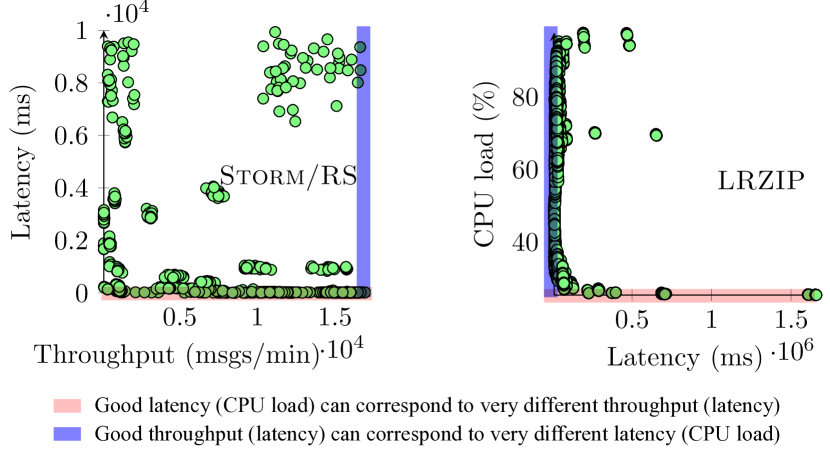
Figure 2: Measured configurations for Storm/RS and LRZIP. The points that Property 3 refers to are highlighted: very good or bad results on one performance objective can both correspond to similarly good value on the other.

3.2 Plain Multi-Objectivization (PMO) Model

A straightforward idea to perform multi-objectivization is to add an auxiliary objective to optimize, along with optimizing the target performance objective. This is what has been commonly used in SBSE scenarios (e.g., [30, 59, 14, 1]). That PMO model can be formulated as:

$$\begin{split}\text{minimize}\begin{cases}f_{t}(\boldsymbol{x})\\ f_{a}(\boldsymbol{x})\\ \end{cases}\end{split}$$ (2)

where $f_{t}(\boldsymbol{x})$ denotes the target performance objective (i.e., the concerned one) and $f_{a}(\boldsymbol{x})$ denotes the auxiliary performance objective.

Putting it in the context of software configuration tuning, the PMO model may cover Property 1, because the natural Pareto relation with respect to the two objectives ensures that the target performance objective is no longer a sole indicator to guide the search. However, it does not fit Property 2 as PMO additionally optimizes the auxiliary performance objective. As such, configurations that perform well on the auxiliary performance objective but poorly on the target performance objective are still regarded as optimal in PMO, despite being meaningless to the original problem. This can result in a significant waste of resources. In addition, PMO does not consider Property 3 as it often assumes conflicting correlation between the two objectives [58, 30], which is hard to assure in software configuration tuning.

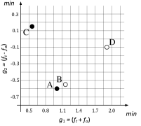
(a) The original target-auxiliary space (i.e. the PMO model)	(b) The meta bi-objective space (i.e. the MMO model)

Figure 3: An illustration of comparison between (a) the PMO model and (b) the MMO model on Storm, where the target performance objective is latency (to minimize) and the auxiliary performance objective is throughput (to maximize). Both of them are normalized and the weight is 1.0 in the MMO model. Let us say $\boldsymbol{A}$, $\boldsymbol{B}$, $\boldsymbol{C}$ and $\boldsymbol{D}$ be a set of four configurations to be considered. Out of them, one needs to select two (e.g., in order to put some better configurations into the next-generation population in a multi-objective optimizer). The solid circle means the configuration being Pareto optimal to the set, and the hollow one is the dominated configuration. Since the PMO model directly minimizes latency and maximizes throughput (Figure 3a), configurations $\boldsymbol{A}$, $\boldsymbol{B}$, and $\boldsymbol{D}$ are Pareto optimal. However, $\boldsymbol{D}$ performs very poorly on latency; preserving it during the search is a waste of resource. In contrast, in the MMO model (Figure 3b), configurations $\boldsymbol{A}$ and $\boldsymbol{C}$ are Pareto optimal. Now comparing configurations $\boldsymbol{C}$ with $\boldsymbol{B}$, since $\boldsymbol{C}$ and $\boldsymbol{A}$ behave much more differently than $\boldsymbol{B}$ and $\boldsymbol{A}$ on the throughput, it is often more likely that they are located on distant regions in the configuration landscape; thus preserving $\boldsymbol{C}$ rather than $\boldsymbol{B}$ (in case $\boldsymbol{A}$ is preserved) is generally more likely to avoid the search being trapped in the local optimum.

3.3 Meta Multi-Objectivization (MMO) Model

Unlike PMO, our meta multi-objectivization (MMO) model creates two meta-objectives based on the performance attributes. The aim is to drive the search towards the optimum of the target performance objective and at the same time, not to be trapped in local optima. In particular, we want to achieve two goals:

• Goal 1: optimizing the target performance objective still plays a primary role, thus no resource waste on, for example, optimizing the auxiliary one (this fits in Property 2);

• Goal 2: but those with different values of the auxiliary performance objective are more likely to be incomparable (i.e., Pareto nondominated), hence the search would not be trapped in local optima (this relates to Properties 1 and 3).

Formally, the MMO model with two meta-objectives $g_{1}(\boldsymbol{x})$ and $g_{2}(\boldsymbol{x})$ is constructed as:

$$\begin{split}\text{minimize}\begin{cases}g_{1}(\boldsymbol{x})=f_{t}(\boldsymbol{x})+w\times f_{a}(\boldsymbol{x})\\ g_{2}(\boldsymbol{x})=f_{t}(\boldsymbol{x})-w\times f_{a}(\boldsymbol{x})\\ \end{cases}\end{split}$$ (3)

whereby each of the two meta-objectives shares the same target performance objective $f_{t}(\boldsymbol{x})$, but differs (effectively being opposite) regarding the auxiliary performance objective $f_{a}(\boldsymbol{x})$. The auxiliary objective can be a readily available one and whose result is of no interest (e.g., throughput or CPU load, in addition to latency). The weight $w$ is a critical parameter that balances the target and auxiliary performance objectives.

To understand the MMO model, Figure 3 gives an example of Storm on how it distinguishes between different configurations, in comparison with the PMO model, where we assume that latency is the target performance objective $f_{t}$ and throughput is the auxiliary performance objective $f_{a}$. Suppose that there is a set of four configurations $\boldsymbol{A}$, $\boldsymbol{B}$, $\boldsymbol{C}$ and $\boldsymbol{D}$. Let us say if we want to select two from them based on their fitness (e.g., in order to put some better configurations into the next-generation population in a multi-objective optimizer, such as NSGA-II). For the PMO model (Figure 3a) that minimizes latency and maximizes throughput, the configuration $\boldsymbol{D}$, which performs extremely poor on latency, will certainly be selected by any multi-objective optimizer, since it is Pareto optimal and also less crowded than the other Pareto optimal configuration $\boldsymbol{A}$ and $\boldsymbol{B}$. In contrast, for the MMO model (Figure 3b) which minimizes the two meta objectives, the two configurations that will be selected are $\boldsymbol{A}$ and $\boldsymbol{C}$ (since they are the only two Pareto optimal ones).

It is worth noting that for the single-objective optimization model (which only considers latency), the two chosen configurations will be $\boldsymbol{A}$ and $\boldsymbol{B}$. However, since $\boldsymbol{C}$ and $\boldsymbol{A}$ behave much more differently than $\boldsymbol{B}$ and $\boldsymbol{A}$ on the throughput, it is more likely that they are located in distant regions in the configuration landscape; thus preserving $\boldsymbol{C}$ rather than $\boldsymbol{B}$ (when $\boldsymbol{A}$ is preserved) is generally more likely to help the search to escape from the local optimum.

In the following, we provide several remarks to help further grasp the characteristics of the MMO model.

Remark 1. The global optimum of the original single-objective problem (i.e., the configuration with the best target performance objective) is Pareto optimal (e.g., the configuration $\boldsymbol{A}$ in the example of Figure 3). This can be derived immediately by contradiction from Equation (3) (the proof is given in the Appendix A).

Remark 2. A similar but more general observation is that a configuration will never be dominated by another that has a worse target performance objective. That is, if configuration $\boldsymbol{x_{1}}$ has a better target performance objective than $\boldsymbol{x_{2}}$ (i.e., $f_{t}(\boldsymbol{x_{1}})<f_{t}(\boldsymbol{x_{2}})$), then whatever their auxiliary performance objective values are, $\boldsymbol{x_{2}}$ will not be better than $\boldsymbol{x_{1}}$ on both $g_{1}$ and $g_{2}$; in the best case for $\boldsymbol{x_{2}}$, they are nondominated to each other (e.g., the configuration $\boldsymbol{B}$ versus $\boldsymbol{C}$ in Figure 3).

Remark 3. The above two remarks apply to the target performance objective, but not to the auxiliary performance objective. This is a key difference from the PMO model, where both objectives hold these remarks. An example of the consequence is the configuration $\boldsymbol{D}$ of Figure 3, which is meaningless to the original problem, but treated as being optimal in PMO and not in MMO.

Remark 4. Our MMO model does not bias to a higher or lower value on the auxiliary performance objective, in contrast to PMO. It makes sense since, as explained in Property 3, we do not know for certain what value of the auxiliary performance objective corresponds to the best target performance objective.

Remark 5. Configurations with dissimilar auxiliary performance objective values tend to be incomparable (i.e., nondominated to each other) even if one is fairly inferior to the other on the target performance objective. For example, the configuration $\boldsymbol{C}$ in Figure 3, which has worse latency than $\boldsymbol{A}$, is not dominated by $\boldsymbol{A}$ as their throughput are rather different. In contrast, the configuration $\boldsymbol{B}$, which even has better latency than $\boldsymbol{C}$, is dominated by $\boldsymbol{A}$, as they are similar on throughput. This enables the model to keep exploring diverse promising configurations during the search, thereby a higher chance to find the global optimum.

Remark 6. If two configurations have the same value of the target performance objective $f_{t}$, then they are always nondominated to each other in the MMO model. This is because the difference between the configurations on the two meta objectives entirely depends on the term related to the auxiliary performance $f_{a}$, which are opposite on the two meta objectives (i.e., $+wf_{a}$ versus $-wf_{a}$); hence a better value of $+wf_{a}$ must have a worse value of $-wf_{a}$. Likewise, configurations with very similar $f_{t}$ are highly likely nondominated to each other.

Remark 7. If two configurations have the same value of auxiliary performance objective $f_{a}$, then they are always subject to dominance relation (i.e., either dominating or being dominated). This is because the difference between the configurations on the two meta objectives entirely depends on the target performance objective $f_{t}$, thereby degenerating a single-objective optimization. Likewise, configurations with very similar $f_{a}$ are high likely comparable to each other.

From Remarks 1–5, we can see that the MMO model is capable of focusing on optimizing the target performance objective (Goal 1) while mitigating the search from being trapped in local optima (Goal 2). In the following sections, on the basis of Remarks 6 and 7, we will explain why and how the weight parameter $w$ in the MMO model can be removed. This will be achieved by amending the normalization method for the model.

3.4 Normalization for MMO Model in the FSE work [26]

Since different performance attributes of the configurable software systems may come with intrinsically different scales, in the FSE work [26], to obtain commensurable $f_{t}(\boldsymbol{x})$ and $f_{a}(\boldsymbol{x})$ we used the following normalization:

$$f(\boldsymbol{x})={{f^{o}(\boldsymbol{x})-f^{o}_{lower}\over{f^{o}_{upper}-f^{o}_{lower}}}}$$ (4)

where $f^{o}(\boldsymbol{x})$ denotes the original value of the configuration $\boldsymbol{x}$ on the performance objective $f$, and $f^{o}_{lower}$ and $f^{o}_{upper}$ are the global lower and upper bounds on that performance objective for the software, respectively. That is, the true scale of the performance objective is used as the bounds.

In practical software configuration tuning, however, $f^{o}_{lower}$ and $f^{o}_{upper}$ are likely to be unknown a priori. Therefore in our FSE work, these bounds are updated by using the maximum and minimum values discovered so far during the tuning to approximate the true scales. Note that using the true scales of the objectives (if known) or their close approximations for normalization is a widely used method in SBSE [86, 69, 78, 29, 3].

3.5 What was Wrong?

The above normalization method can be effective, but with one undesired implication: it makes the weight $w$ in the MMO model become a highly sensitive parameter, and consequently finding the right setting for a system requires much effort of trial and error. In [26] and this work (Section 5), we examined a wide range of the weight settings for MMO model (i.e., $0.01,0.1,0.3,0.5,0.7,0.9,1.0,10$). A key finding is that the weight achieving the best performance differs drastically on different configurable software systems: some systems work better with a tiny weight value, e.g., $w=0.01$ for the latency of Storm under the WordCount benchmark, while some others do best with a big value, e.g., $w=10$ for the iteration count of Trimesh.

The reason for this occurrence is the severe discrepancy between the range of the current search population and the objectives’ scales in software configuration tuning. If the target performance objective in the population evolves into a range that is tiny compared to its objective scale in the whole search space (while the auxiliary performance objective does not), then the values of the target performance objective of configurations in the current population after the normalization (Equation 4) will be very close. In this case, the auxiliary performance objective will play a dominant role, and all the configurations are highly likely nondominated to each other in the MMO model (see Remark 6). Figure 4 gives such an example, where we visualize an intermediate population of MMO model (with the normalization from the FSE work) during the tuning for Storm/WC. As can be seen in Figure 4b, since the range of the target performance objective (latency) in the population becomes “very small” (around $[95ms,1800ms]$), compared to the objective scale ($[3ms,55209ms]$), after the normalization the values of the target performance objective become tiny, condensing in the range of $[0,0.03]$ only. The auxiliary performance objective (throughput), in contrast, are more evenly spread over the range of $[0,1]$ after the normalization. This leads to all the configurations in the population being non-dominated to each other within the transformed space of our MMO model (Figure 4c). Unfortunately, all configurations in the population being nondominated is detrimental to the search since there is no selection pressure (i.e., discriminative power); everyone is incomparable even the one with the best target performance objective.

Likewise, if the auxiliary performance objective of the configurations in the population shrinks into a range that is tiny compared to its true objective scale in the whole search space (while the target performance objective does not), then the auxiliary objective of configurations in the population after the normalization will be very close. Here, the target performance objective will play a dominant role, and all the configurations are highly likely comparable in terms of Pareto dominance in the MMO model (Remark 7). Figure 5 gives such an example, where we illustrate an intermediate population of MMO model (with the normalization from the FSE work) during the tuning for LRZIP. As can be seen from Figure 5b, since the range of auxiliary performance objective in the population becomes “very small” (around $[1.03\times 10^{4}ms,1.3\times 10^{4}ms]$), compared to the objective scale ($[10^{4}ms,1.7\times 10^{6}ms]$, after the normalization the auxiliary performance objective’s values become tiny, condensing in the range of $[0,1.7\times 10^{-3}]$ only. This leads to all the configurations in the population being either dominating or dominated by each other within the transformed space of our MMO model (Figure 5c), which effectively means that the problem degenerates to the original single-objective problem, where the configurations are discriminative virtually based on their target performance objective (thus easily being trapped in local optima).

(a) Original

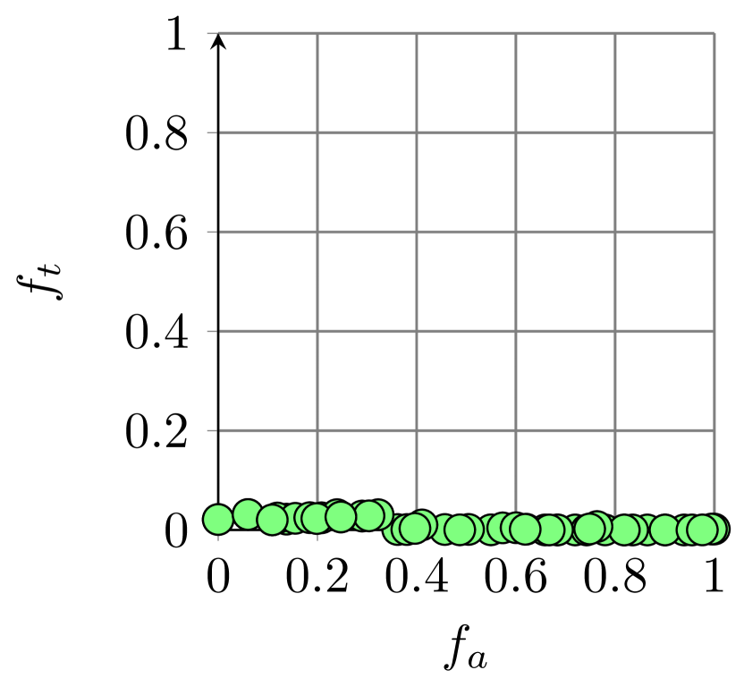
(b) Normalized

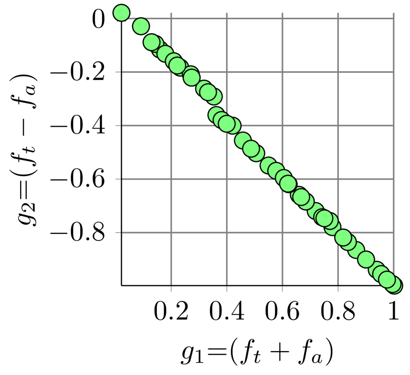
(c) In the MMO space

Figure 4: An intermediate population of configurations for Storm/WC generated by our MMO model with the normalization method from FSE work [26] on top of NSGA-II.

(a) Original

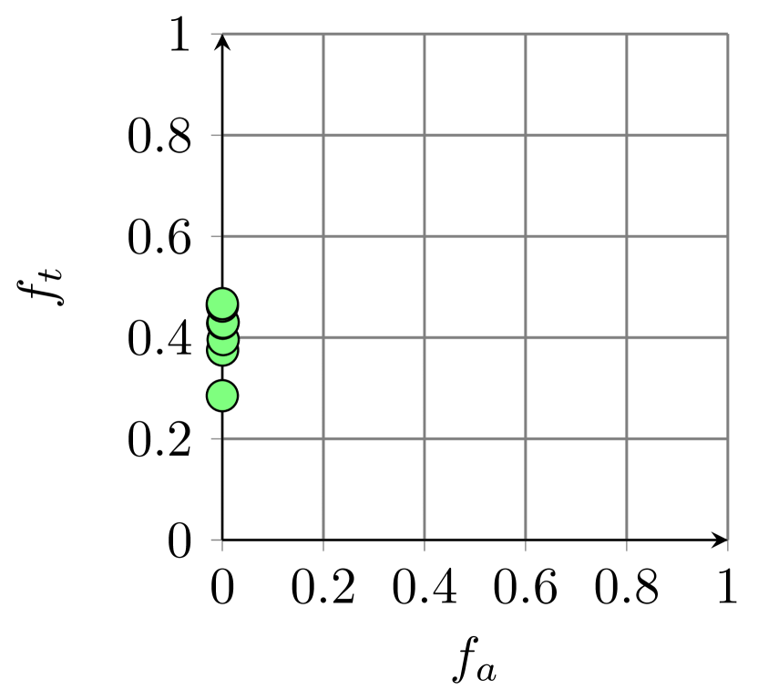
(b) Normalized

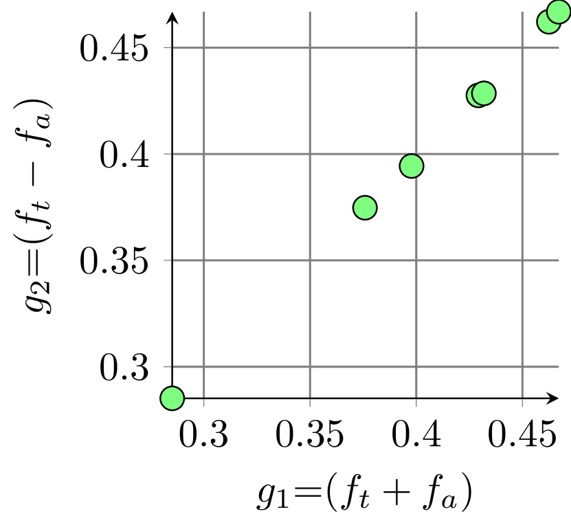
(c) In the MMO space

Figure 5: An intermediate population of configurations for LRZIP generated by our MMO model with the normalization method from FSE work [26] on top of NSGA-II.

3.6 A New Normalization

The above observations suggest that the normalization based on the (approximate) true scales of the performance objectives may not be suitable for the MMO model. Fortunately, this can be fixed by considering the current population as the basis of bounds in the normalization. That is, we replace Equation 4 with the following:

$$f(\boldsymbol{x})={{f^{o}(\boldsymbol{x})-f^{o}_{min}}\over{f^{o}_{max}-f^{o}_{min}}}$$ (5)

where $f^{o}(\boldsymbol{x})$ denotes the original value of the configuration $\boldsymbol{x}$ on the objective $f$, and $f^{o}_{min}$ and $f^{o}_{max}$ are the maximum and minimum values of the current population on the objective $f$, respectively. As such, instead of using the global bounds throughout the search, the local bounds (in the population of configurations of every generation along with the evolution) are used in the normalization.

With this modification, the values of the target and auxiliary performance objectives of configurations in the population are likely to be distributed in the range of $[0,1]$. This results in a mixed population that consists of both comparable and incomparable configurations, thus striking a good balance between imposing the selection pressure towards the best target performance objective while preserving the diversity of the auxiliary performance objective.

(a) Original

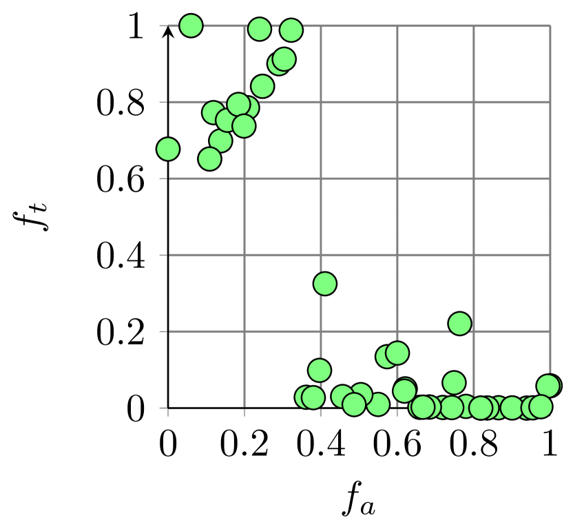
(b) Normalized

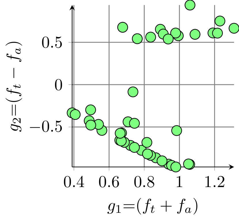
(c) In the MMO space

Figure 6: The same population of Figure 4 under the MMO model with the new normalization method proposed in this work.

(a) Original

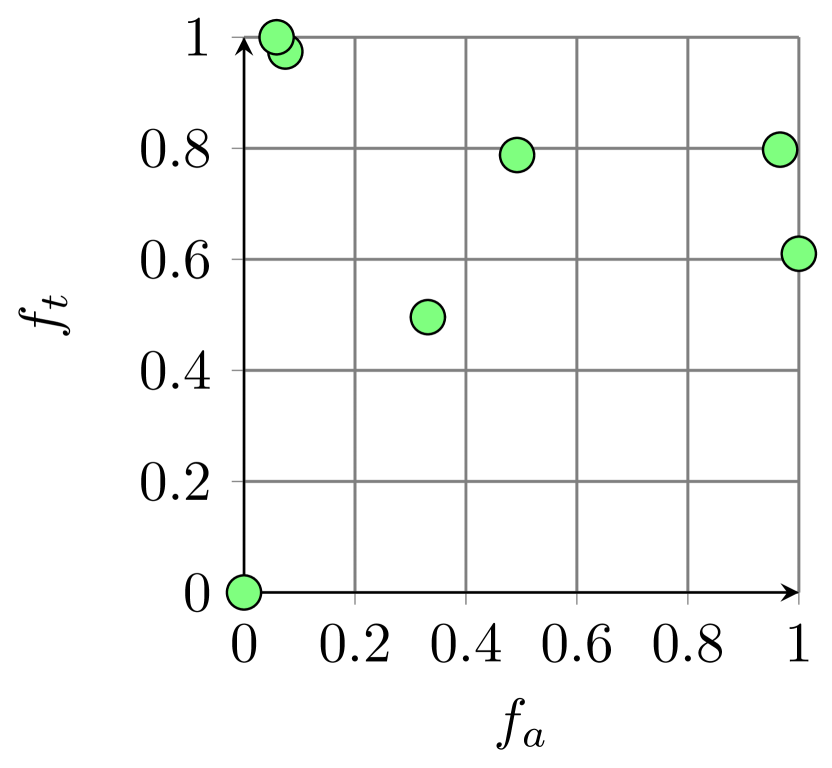
(b) Normalized

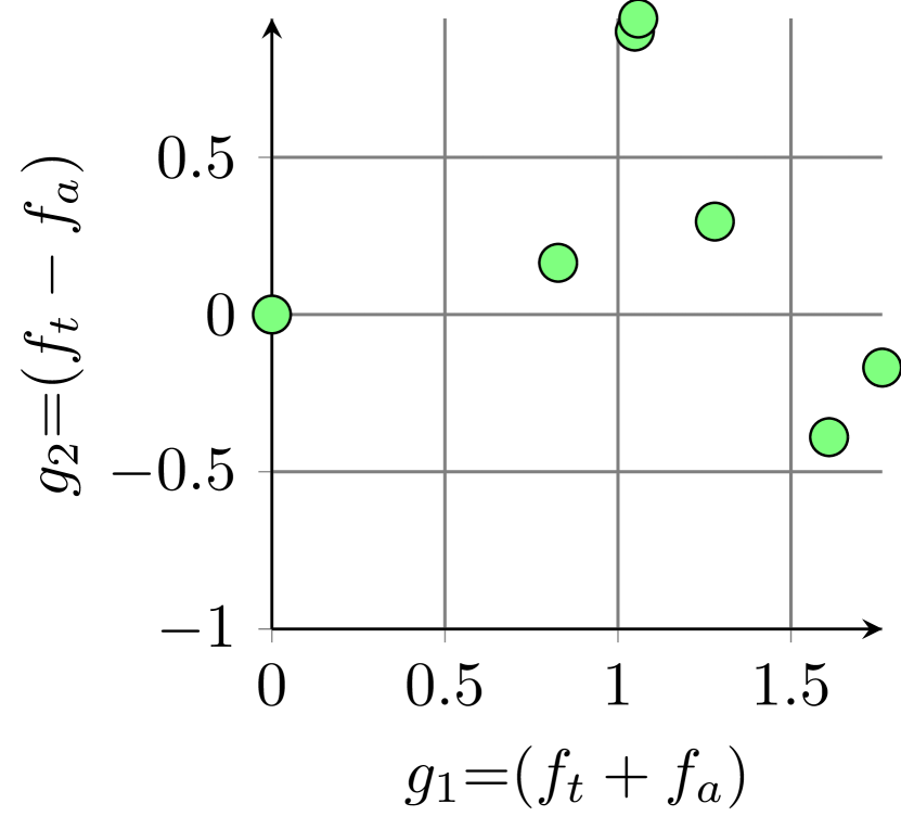
(c) In the MMO space

Figure 7: The same population of Figure 5 under the MMO model with the new normalization method proposed in this work.

Figures 6 and 7 give the results of the examples from Figures 4 and 5 after the new normalization is implemented, respectively. As can be seen, the configurations in the population after the normalization do not concentrate into one value on either objective (Figures 6b and 7b), and in our MMO space there now exist both dominated and nondominated configurations in the population (Figures 6c and 7c). In this case, we are able to remove the weight in the MMO model (i.e., setting $w=1$ for all cases), since the two performance objectives after the normalization are always commensurable. This normalization amounts to a dynamic adaptation of the two performance objectives’ contributions during the search, which plays a similar role of choosing a proper weight to balance them in our FSE work.

3.7 Integrating with an Optimizer

Since MMO model is an optimization model, it can fit with different population-based multi-objective optimizers such as NSGA-II. A pseudo-code for using the MMO model with the normalization on top of NSGA-II has been demonstrated in Algorithm 1. As can be seen, there are merely two amendments required (the red crossed statements are the code for the FSE work and the green ones are the code changed in this work):

1. Keeping track of the bounds on $f_{t}(\boldsymbol{x})$ and $f_{a}(\boldsymbol{x})$ for normalizing both the target and auxiliary performance objectives (lines 4–5 and 20–21). The definitions of those bounds differ depending on the normalization methods, i.e., with lines 20–21 instead of lines 19–19, the bounds are locally restricted to the current population or otherwise they would be the global bounds so far.

2. Performing the normal Pareto search procedure in NSGA-II within the transformed meta bi-objective space ($g_{1}(\boldsymbol{x})$ and $g_{2}(\boldsymbol{x})$) of MMO model without a weight, instead of the original target-auxiliary space ($f_{t}(\boldsymbol{x})$ and $f_{a}(\boldsymbol{x})$), as shown at lines 8, 13, 25, and 27.

4 Experimental Evaluation

1

Input: Configuration space $\mathcal{V}$; the system $\mathcal{F}$; weight $w$

2

Output: ${s}_{best}$ the best configuration on $f_{t}(\boldsymbol{x})$

Declare: bound vectors $\mathbf{\overline{z}_{max}}$ and $\mathbf{\overline{z}_{min}}$

3 Randomly initialize a population of $n$ configurations $\mathcal{P}$

4

5$\mathbf{\overline{z}_{max}}=\emptyset$; $\mathbf{\overline{z}_{min}}=\emptyset$

6 /* measuring $f_{t}$ and $f_{a}$ for configurations in $\mathcal{P}$ on the system */

7 measure($\mathcal{P},\mathcal{F}$)

8

9/* initializing the bounds for normalization */

10 $\mathbf{\overline{z}_{max}}=$ updateUpperBounds($\mathcal{P}$)

11 $\mathbf{\overline{z}_{min}}=$ updateLowerrBounds($\mathcal{P}$)

12

13/* updating $g_{1}$ and $g_{2}$ */

14 computeMMOModel($w,\mathcal{P},\mathbf{\overline{z}_{max}},\mathbf{\overline{z}_{min}}$)

15 computeMMOModel($\mathcal{P},\mathbf{\overline{z}_{max}},\mathbf{\overline{z}_{min}}$)

16

17while The search budget is not exhausted do

18      

19      $\mathcal{P^{\prime}}=\emptyset$

20      

21      while $\mathcal{P^{\prime}}<n$ do

22             /* selecting parents based on $g_{1}$ and $g_{2}$ */

23             $\{{s}_{x},{s}_{y}\}\leftarrow$mating($\mathcal{P}$)

24            $\{{o}_{x},{o}_{y}\}\leftarrow$doCrossoverAndMutation($\mathcal{V},{s}_{x},{s}_{y}$)

25             /* measuring $f_{t}$ and $f_{a}$ for configurations ${o}_{x}$ and ${o}_{y}$ on the system (if unique) */

26             measure(${o}_{x},{o}_{y},\mathcal{F}$)

27             $\mathcal{P^{\prime}}\leftarrow\mathcal{P^{\prime}}\bigcup\{{o}_{x},{o}_{y}\}$

28            

29      /* the bounds are reset based on the current population at each generation regardless of the previous bound values */

30      

31      $\mathbf{\overline{z}_{max}}=$ updateUpperBounds($\mathcal{P},\mathbf{\overline{z}_{max}}$)

32       $\mathbf{\overline{z}_{min}}=$ updateLowerrBounds($\mathcal{P},\mathbf{\overline{z}_{min}}$)

33      

34      $\mathbf{\overline{z}_{max}}=$ updateUpperBounds($\mathcal{P}$)

35       $\mathbf{\overline{z}_{min}}=$ updateLowerrBounds($\mathcal{P}$)

36      

37      $\mathcal{U^{\prime}}\leftarrow$$\mathcal{P}\bigcup\mathcal{P^{\prime}}$

38      

39      /* updating $g_{1}$ and $g_{2}$ */

40       computeMMOModel($w,\mathcal{U^{\prime}},\mathbf{\overline{z}_{max}},\mathbf{\overline{z}_{min}}$)

41       computeMMOModel($\mathcal{U^{\prime}},\mathbf{\overline{z}_{max}},\mathbf{\overline{z}_{min}}$)

42       /* sorting based on $g_{1}$ and $g_{2}$ */

43       $\mathcal{U}\leftarrow$nondominatedSorting($\mathcal{U^{\prime}}$)

44       $\mathcal{P}\leftarrow$top $n$ configurations from $\mathcal{U}$

45

46return ${s}_{best}\leftarrow$bestConfiguration($\mathcal{P}$)

Algorithm 1 MMOonNSGA-II

In this section, we articulate the experimental methodology for evaluating our MMO model with the new normalization. To better distinguish this work and the FSE work [26], we use the following terminology:

• MMO-FSE: this refers to our MMO model with the normalization method from the FSE work.

• MMO: this refers to our MMO model with the new normalization proposed in this work.

All optimization models and optimizers are implemented in Java, using jMetal [32] and Opt4J [56].

TABLE I: Configurable software systems studied.

Software System	Domain	Performance Objectives		$\#$ Options	Search Space	Used By
MariaDB	SQL database	O1: latency	O2: CPU load	10	864	[64]
Storm/WC	stream processing	O1: throughput	O2: latency	6	2,880	[60, 43, 64]
VP9	video encoding	O1: latency	O2: CPU load	12	3,008	[64]
Storm/RS	stream processing	O1: throughput	O2: latency	6	3,839	[60, 43, 64]
LRZIP	file compression	O1: latency	O2: CPU load	12	5,184	[64]
MongoDB	no-SQL database	O1: latency	O2: CPU load	15	6,840	[64]
Keras-DNN/SA	deep learning	O1: AUC	O2: inference time	12	16,384	[57, 44]
Keras-DNN/Adiac	deep learning	O1: AUC	O2: inference time	12	24,576	[57, 44]
x264	video encoding	O1: PSNR	O2: energy usage	17	53,662	[60, 71, 64]
LLVM	compiler	O1: latency	O2: CPU load	16	65,436	[60, 64]
Trimesh	triangle mesh	O1: $\#$ iteration	O2: latency	13	239,260	[60, 71]

4.1 Research Questions

Our experiment investigates the following research questions (RQs):

• RQ1: How effective is the MMO?

As the most fundamental question, we ask RQ1 to verify whether our MMO can better help to mitigate the issue of local optima, i.e., by providing better results than the MMO-FSE, PMO, and state-of-the-art single-objective counterparts. However, even if the MMO can lead to promising results by mitigating local optima, it would be less useful if it requires a significantly large amount of resources to do so. Under the same settings as RQ1, our second research question is, therefore:

• RQ2: How resource-efficient is the MMO?

In RQ2, we are interested to examine whether the MMO can utilize the resource (the number of measurements) efficiently when reaching a certain level of performance.

One of the key novelties for MMO, compared with MMO-FSE, is parameter-free. Yet, this would be meaningless if the MMO-FSE achieves similarly promising results over different weights on the systems studied; or the effort for finding the best weight is trivial. Hence, our next RQ is:

• RQ3: How meaningful is the parameter-free design in MMO?

RQ3 seeks to understand two aspects: (1) how does MMO perform when compared with MMO-FSE under different weights; and (2) How much extra resource is required for one to tune the MMO-FSE for finding a promising weight value.

To reduce unnecessary noise, we investigate RQ1-3 by directly measuring the systems, which belongs to the measurement-based tuning methods for software configuration tuning [61, 90, 83]. However, there exist studies leveraging on the model-based tuning methods where a surrogate is built to serve as a cheap evaluator to predict the performance of a configuration, under the assumption of the single-objective model. Since the key difference between measurement-based and model-based tuning methods lies in whether a surrogate is used to guide the search, the MMO, which itself is an optimization model, can be considered complementary to the model-based alternative. Therefore, our final research question is concerned with:

• RQ4: Can MMO consolidate the existing model-based tuning method?

To that end, we extend Flash [60] — a recent tool from the Software Engineering community for configuration tuning — with our MMO and examine whether its performance can be improved.

4.2 Software Systems

As shown in Table I, we experiment on 11 real-world software systems and environments that have been commonly used in prior work [60, 43, 57, 44, 64]. They come from diverse domains, e.g., SQL database, video encoding, and stream processing, while having different performance attributes, scale, and search space of valid configurations. Each software system has two performance objectives, which are chosen from prior work [60, 43, 57, 44, 64]. In all experiments, we use each of their two performance attributes as the target performance objective in turn while the other serves as the auxiliary performance objective, leading to 22 cases in total. We apply the same configuration options and their ranges as studied previously since those have been shown to be the key ones for the software systems under the related environment.

Noteworthily, it can be rather expensive even for a single measurement under those systems, e.g., it may take up to 341 seconds to measure a configuration on MongoDB. To ensure realism and expedite the experiments, we use the data of those systems collected by existing work; these datasets cover the whole search space and each measurement is extracted from 3-5 repeats [43, 64].

4.3 Settings for RQ1, RQ2, and RQ3

4.3.1 Optimizers

For the single-objective optimization model, we examine four state-of-the-art optimizers that are widely used in software configuration tuning, all of which deal with local optima in different ways:

• Random Search (RS) with a high neighbourhood radius to escape from the local optima, as used in [7, 87, 61].

• Stochastic Hill Climbing with restart (SHC-r), which is exploited by [83, 52], aiming to avoid local optima by using different starting points.

• Single-Objective Genetic Algorithm (SOGA) from [6, 69, 67, 73] that seeks to escape local optima by using variation operators.

• Simulated Annealing (SA) that tackles local optima by stochastically accepting inferior configurations as used in [34, 35].

While the MMO does not tie to any specific multi-objective optimizer, we use NSGA-II for the MMO, MMO-FSE, and PMO in this work, because (1) it has been predominately used for software configuration tuning in prior work when multiple performance attributes are of interest [25, 72, 28, 48, 74]; (2) it shares many similarities with the SOGA that we compare in this work. However, it is worth noting that MMO may not be able to work with some multi-objective optimizers specifically designed for SBSE problems where the objectives are not treated equally, such as [62, 38, 37].

4.3.2 Weight Values for MMO-FSE

In our experiments, we evaluate a set of weight values, i.e., $w\in\{0.01,0.1,0.3,0.5,0.7,0.9,1.0,10\}$, for the MMO-FSE. Those are merely pragmatic settings without any sophisticated reasoning. In this way, we aim to examine whether the MMO-FSE can perform as well as MMO under the best weight chosen from a set of diverse weight values (or indeed worse on all of them).

TABLE II: Measurement search budgets and population sizes.

Software	Size	Budget	Software	Size	Budget
MariaDB	20	400	Storm/WC	50	600
VP9	30	700	Storm/RS	50	900
LRZIP	20	400	MongoDB	20	500
Keras-DNN/SA	20	400	Keras-DNN/Adiac	20	400
x264	50	2,500	LLVM	20	600
Trimesh	20	1,000

4.3.3 Search Budget

In this work, we use the number of measurements to quantify the search budget and resource consumed, as it is language-/platform-independent and does not suffer from the interference cause by the background processes of the operating system.

Since our goal is to examine how badly a model/optimizer can suffer from trapping at undesired local optima when tuning software configuration, it is important to study the result under reasonable convergence, i.e., increasing the search budget is unlikely to change the outcomes. To that end, for every optimizer/model on each system (and its performance objectives), we examine different search budgets from $\{100,200,...,X\}$ where $X$ refers to the smaller one between $3,000$ and the size of the search space. The purpose is to set a search budget as the smallest number of measurements for all optimizers/models, such that they all have less than 10% changes of configuration within the last 10% of the measurement count. However, to ensure the realism of the setting, we make sure that the actual time taken for exhausting the search budget does not exceed 48 hours for a run overall. The identified search budgets are then used as the termination criterion in our experiments, as shown in Table II. It is worth noting that the search budget identified remains much smaller than the corresponding search space. For example, it only allows for measuring 0.42% of the configurations for Trimesh.

Since each measurement has considered the noise [43, 64] and only the profiling of systems would be expensive in practice, in each run, we cached the measurement of every distinct configuration, which can be reused directly when the same configuration appears again during the tuning. In other words, only the distinct configurations would consume the budget.

To account for the stochastic nature of the optimizers, we repeat all experiments 50 runs under the search budget.

4.3.4 Other Parameters

For the other key parameters of the optimizers, we apply the binary tournament for mating selection, together with the boundary mutation and uniformed crossover in SOGA and NSGA-II, as used in prior work [25, 69, 28]. The mutation and crossover rates are set to 0.1 and 0.9, respectively, as commonly set in software configuration tuning [25].

However, what we could not decide easily is the population size for SOGA and NSGA-II. Therefore, for each software system, we additionally examine a set of population sizes, i.e., $\{10,20,...,100\}$, under the search budget identified previously. Similarly, we set the largest population size that can still ensure there are less than 10% changes of configurations at the last 10% of the measurement count. The results are shown in Table II. In this way, we seek to reach a good balance between convergence (smaller population change) and diversity (larger population size) under a search budget.

1

Input: Configuration space $\mathcal{V}$; the system $\mathcal{F}$

2

Output: ${s}_{best}$ the best configuration on $f_{t}(\boldsymbol{x})$

Declare: vector of surrogates $\mathcal{M}$ (one for each performance objective)

3 Randomly initialize a size of $k$ configurations $\mathcal{P}$

4 measure($\mathcal{P},\mathcal{F}$)

5 /* removing measured configurations */

6 $\mathcal{V}\leftarrow$$\mathcal{V}-\mathcal{P}$

7 while The search budget is not exhausted do

8       $\mathcal{M}=$ CARTs($\mathcal{P}$)

9       /* searching an estimated-best configuration for measurement */

10       ${o}=$ search($\mathcal{V},\mathcal{M}$)

11       measure(${o},\mathcal{F}$)

12       $\mathcal{V}\leftarrow$$\mathcal{V}-{o}$

13       $\mathcal{P}\leftarrow$$\mathcal{P}+{o}$

14       if ${o}$ is measured to be better than ${s}_{best}$ on $f_{t}(\boldsymbol{x})$ then

15             ${s}_{best}={o}$

16            

17      

18

19return ${s}_{best}$

Algorithm 2 Flash

4.4 Settings for RQ4

4.4.1 Optimizers

For model-based tuning methods, we consider Flash [60] in this work, because (1) it is a recent effort from the Software Engineering community that tackles the general software configuration tuning problem, as opposed to some of the others that have been tailored to a specific domain, e.g., machine learning algorithms [57]; (2) it has been designed to take the rugged and sparse search space into account, which is one of the key properties for the problem; (3) it has been tested on some of the systems studied in this work, e.g., x264.

In a nutshell, Flash was derived from the Sequential Model-Based Optimization (SMBO) paradigm, which is a generalization of the Bayesian Optimization (BO) [70]. As shown in Algorithm 2, the basic idea is to build a surrogate that learns the correlation between configurations and their values of a performance objective (line 6). Such a surrogate is then used to guide the search to decide which promising configuration to measure next via an acquisition function (line 8), after which the surrogate would be updated by using the newly measured configuration. Like other measurement-based tuning methods, the process terminates when the search budget is exhausted. Yet, unlike the classic BO, Flash does two major changes for the problem to tune a single performance objective:

1. The surrogate is a CART [12] instead of the classic Gaussian Process in BO [70].

2. The acquisition function no longer considers uncertainty but solely targets for the best-predicted performance value.

Note that Flash originally uses an exhaustive search to find the best-predicted configuration at each sampling iteration (line 8), but this may not be ideal for our study because of two reasons: (1) exhaustively traversing the whole configuration space itself is still a lengthy process especially on some of the large systems. For example, on each iteration for Trimesh, it can take several minutes on a standard machine to run even for a surrogate. (2) Since the surrogate is not always accurate [90], the exhaustive search could amplify the side-effects caused by the errors in misleading the search. Therefore, we replace the exhaustive search with a random search, which works well and has been recommended as a replacement for SMBO [7].

4.4.2 Search Budget

To ensure fairness, we set the same search budget as used in the original work of Flash [60], i.e., 50 measurements. Further, we also use the same initial sample size ($k=30$ in Algorithm 2) to pre-train the surrogate. As for the search process with the surrogate, we allow for 1,000 surrogate evaluations (including redundant ones) which is a typical setting from the other work for optimizing the surrogate when an exhaustive search is undesirable [45, 65].

Similar to RQ1-3, each experiment is repeated 50 runs.

4.5 Statistical Validation

We use the following methods for pairwise statistical test:

• Non-parametric test: To verify statistical significance, we leverage the Wilcoxon test [82] — a widely used non-parametric test for SBSE and has been recommended in software engineering research for its strong statistical power on pairwise comparisons [5]. The standard $a=0.05$ is set as the significance level over 50 runs. If the resulted $p<0.05$, we say the magnitude of differences in the comparisons is significant. We use either the paired (Wilcoxon signed-rank) or non-paired (Wilcoxon rank-sum) version as appropriate.

• Effect size: To ensure the resulted differences are not generated from a trivial effect, we use $\hat{A}_{12}$ [81] to verify the effect size of the comparisons on target performance objectives over 50 runs. According to Vargha and Delaney [81], when comparing our MMO and its counterpart in this work, $\hat{A}_{12}>0.5$ denotes that the MMO is better for more than 50% of the times. In particular, $0.56\leq\hat{A}_{12}<0.64$ indicates a small effect size while $0.64\leq\hat{A}_{12}<0.71$ and $\hat{A}_{12}\geq 0.71$ mean a medium and a large effect size, respectively.

As such, we say a comparison is statistically significant only if it has $\hat{A}_{12}\geq 0.56$ (or $\hat{A}_{12}\leq 0.44$) and $p<0.05$.

TABLE III: Comparing MMO with the other state-of-the-arts over 50 runs. SO_best and MMO-FSE_best denote the best single-objective model/optimizer and the MMO-FSE with the best weight, respectively. max width=.1 shows the average and standard error (SE) on the target performance objective achieved (all objective values are normalized within $[0,1]$ and the closer to the left, the better). max width=.1 denotes the best average among others. Column “$\hat{A}_{12}$ ($p$ value)” shows the $\hat{A}_{12}$ and $p$ value when comparing the corresponding counterpart with MMO. The blue cells denote MMO wins while red cells mean it loses; otherwise it is a tie. Statistically significant comparisons, i.e., $\hat{A}_{12}\geq 0.56$ ($\hat{A}_{12}\leq 0.44$) and $p<0.05$ are highlighted in bold.

max width = 1

Mean/SE $\hat{A}_{12}$ ($p$ value) SObest max width=.1 .66 ($=$.005) MMO-FSEbest max width=.1 .43 ($=$.197) PMO max width=.1 .65 ($=$.011) MMO max width=.1 -		Mean/SE $\hat{A}_{12}$ ($p$ value) max width=.1 .51 ($=$.899) max width=.1 .53 ($=$.608) max width=.1 .71 ($<$.001) max width=.1 -		Mean/SE $\hat{A}_{12}$ ($p$ value) max width=.1 .55 ($=$.366) max width=.1 .46 ($=$.491) max width=.1 .66 ($=$.005) max width=.1 -		Mean/SE $\hat{A}_{12}$ ($p$ value) max width=.1 .50 ($=$1.00) max width=.1 .99 ($<$.001) max width=.1 .66 ($=$.006) max width=.1 -
(a). MariaDB-O1		(b). MariaDB-O2		(c). Storm/WC-O1		(d). Storm/WC-O2
Mean/SE $\hat{A}_{12}$ ($p$ value) SObest max width=.1 .64 ($=$.016) MMO-FSEbest max width=.1 .44 ($=$.279) PMO max width=.1 .89 ($<$.001) MMO max width=.1 -		Mean/SE $\hat{A}_{12}$ ($p$ value) max width=.1 .64 ($=$.018) max width=.1 .48 ($=$.754) max width=.1 .87 ($<$.001) max width=.1 -		Mean/SE $\hat{A}_{12}$ ($p$ value) max width=.1 .57 ($=$.228) max width=.1 .52 ($=$.720) max width=.1 .90 ($<$.001) max width=.1 -		Mean/SE $\hat{A}_{12}$ ($p$ value) max width=.1 .50 ($=$1.00) max width=.1 .94 ($<$.001) max width=.1 .53 ($=$.605) max width=.1 -
(e). VP9-O1		(f). VP9-O2		(g). Storm/RS-O1		(h). Storm/RS-O2
Mean/SE $\hat{A}_{12}$ ($p$ value) SObest max width=.1 .62 ($=$.035) MMO-FSEbest max width=.1 .77 ($<$.001) PMO max width=.1 .89 ($<$.001) MMO max width=.1 -		Mean/SE $\hat{A}_{12}$ ($p$ value) max width=.1 .55 ($=$.365) max width=.1 .77 ($<$.001) max width=.1 .81 ($<$.001) max width=.1 -		Mean/SE $\hat{A}_{12}$ ($p$ value) max width=.1 .74 ($<$.001) max width=.1 .54 ($=$.535) max width=.1 .59 ($=$.122) max width=.1 -		Mean/SE $\hat{A}_{12}$ ($p$ value) max width=.1 .63 ($=$.031) max width=.1 .64 ($=$.018) max width=.1 .60 ($=$.076) max width=.1 -
(i). LRZIP-O1		(j). LRZIP-O2		(k). MongoDB-O1		(l). MongoDB-O2
Mean/SE $\hat{A}_{12}$ ($p$ value) SObest max width=.1 .63 ($=$.023) MMO-FSEbest max width=.1 .54 ($=$.493) PMO max width=.1 .48 ($=$.684) MMO max width=.1 -		Mean/SE $\hat{A}_{12}$ ($p$ value) max width=.1 .62 ($=$.037) max width=.1 .94 ($<$.001) max width=.1 .61 ($=$.049) max width=.1 -		Mean/SE $\hat{A}_{12}$ ($p$ value) max width=.1 .65 ($=$.012) max width=.1 .54 ($=$.517) max width=.1 .55 ($=$.395) max width=.1 -		Mean/SE $\hat{A}_{12}$ ($p$ value) max width=.1 .64 ($=$.015) max width=.1 .99 ($<$.001) max width=.1 .81 ($<$.001) max width=.1 -
(n). Keras-DNN/SA-O1		(m). Keras-DNN/SA-O2		(o). Keras-DNN/Adiac-O1		(p). Keras-DNN/Adiac-O2
Mean/SE $\hat{A}_{12}$ ($p$ value) SObest max width=.1 .69 ($=$.001) MMO-FSEbest max width=.1 .45 ($=$.370) PMO max width=.1 .67 ($=$.004) MMO max width=.1 -		Mean/SE $\hat{A}_{12}$ ($p$ value) max width=.1 .61 ($=$.049) max width=.1 .52 ($=$.762) max width=.1 .72 ($<$.001) max width=.1 -		Mean/SE $\hat{A}_{12}$ ($p$ value) max width=.1 .50 ($=$1.00) max width=.1 .50 ($=$1.00) max width=.1 .52 ($=$.730) max width=.1 -		Mean/SE $\hat{A}_{12}$ ($p$ value) max width=.1 .62 ($=$.043) max width=.1 .59 ($=$.107) max width=.1 .78 ($<$.001) max width=.1 -
(q). x264-O1		(r). x264-O2		(s). LLVM-O1		(t). LLVM-O2
Mean/SE $\hat{A}_{12}$ ($p$ value) SObest max width=.1 .50 ($=$1.00) MMO-FSEbest max width=.1 .50 ($=$1.00) PMO max width=.1 .50 ($=$1.00) MMO max width=.1 -		Mean/SE $\hat{A}_{12}$ ($p$ value) max width=.1 .66 ($=$.005) max width=.1 .52 ($=$.672) max width=.1 .81 ($<$.001) max width=.1 -	% Win % Lose % Tie MMO vs. SObest 82% 0% 18% MMO vs. MMO-FSEbest 67% 23% 10% MMO vs. PMO 90% 5% 5%
(u). Trimesh-O1		(v). Trimesh-O2	(w). Overall % win/loss/tie for MMO versus the others

5 Results

In this section, we present and discuss the experiment results. All code and data can be accessed at: https://github.com/ideas-labo/mmo.

5.1 RQ1: Effectiveness

5.1.1 Method

To answer RQ1, we compare MMO with the state-of-the-art single-objective counterparts (as discussed in Section 4.3.1), as well as the MMO-FSE and PMO, over all the 22 cases of study. Since the best single-objective optimizer (denoted as SO_best) and the MMO-FSE with the best weight (denoted as MMO-FSE_best) differ across the cases., we use the following procedure to select the best representative in each case:

1. Run all candidates under the full-scale experiment.

2. Rank the results using Scott-Knott test [68] according to the target performance objective.

3. Select the one with the best rank; if there are multiple candidates under the best rank, the one with the best average (over 50 runs) on the target performance objective would be used.

To ensure statistical significance, the statistical test and effect size are reported for every pairwise comparison between our MMO and the other counterparts over 50 runs.

5.1.2 Findings

From Table III, we can see that MMO performs considerably better than the best single-objective counterpart SO_best, winning 18 out of 22 cases within which 14 of them show statistical significance ($\hat{A_{12}\geq 0.56}$ and $p<0.05$); the remaining 4 cases are all tie and no cases of loses. The magnitudes of gains are also clear. The improvements over PMO are also clear: MMO wins 20 cases (15 have statistically significant differences) under mostly large magnitude of gains; there are also one tie and one lose.

When comparing to the MMO-FSE with the best weight (MMO-FSE_best), MMO wins 15 out of the 22 cases with 10 of them showing statistical significance; loses on 5 cases with no statistically significant ones, together with two ties. This means that, although MMO-FSE_best is competitive, MMO can still obtain further improvement in general thanks to the new normalization method. This is especially true in some cases, such as Storm/RS-O2, where the target performance objective values are much more skewed than the auxiliary ones (recall from Figure 4). Even though MMO-FSE_best was pre-tuned with some best weights, such finding is not surprising because: firstly, the given set of weights may not be exhaustive. Indeed, as we will show in the next section, the weight tuning itself can be profoundly expensive, making exhaustive search unrealistic. As such, the chosen weight may still be far from the truly optimal weight setting. Secondly, as the population evolves, the objective values keep changing, particularly on the target performance objective. A fixed weight typically does not stay ideal during the entire evolution process. For example, the weight may be a good fit at the beginning of the evolution when the population has a relatively large range of the target performance objective values, but it may become unsuitable when the population converges into a tiny region with respect to the target performance objective.

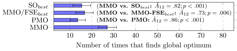
Figure 8: The number of times to find the global optimum within 50 runs for all cases. The reported figures are the average and standard error across all cases. For all statistical comparisons with MMO, $\hat{A}_{12}>.50$ means MMO wins.

To examine whether MMO can indeed improve the chances for reaching the global optimum of the target performance objective, in Figure 8, we plot the average number of runs that each model/optimizer reaches the global optimum across all cases. We see that, as expected, MMO cannot find the global optimum for all runs under the systems studied. However, in general, it hits the global optimum more regularly than the others with statistical significance.

To understand why our MMO can outperform the state-of-the-arts, we took a closer look into the configurations explored during the runs. We identified two most common patterns shown in Figure 9. As can be seen from Figure 9a, the first pattern is where MMO reaches the global optimum while the others do not; the second represents a run where the global optimum has never been found, but MMO produces a result that is much closer to it than that of the others, as shown in Figure 9b. It is worth noting that, under both patterns, there exist some large regions of local optima that cause the others to suffer more than MMO. This is evident by Figure 9 where the highlighted local optima regions are mostly crowded with points explored by the other counterparts. The MMO, in contrast, escapes from these local optima by exploring an even larger area while keeping the tendency towards better target performance objective, which is precisely our Goals 1 and 2 from Section 3.

In summary, we can answer RQ1 as:

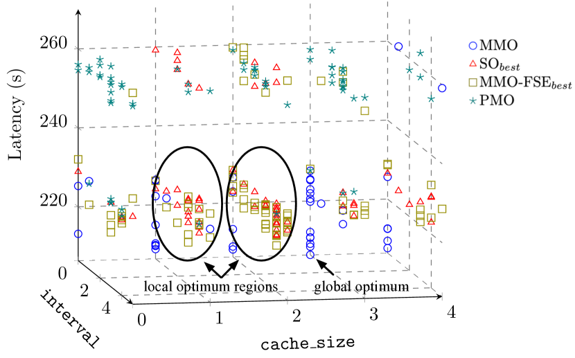
(a) MongoDB-O1

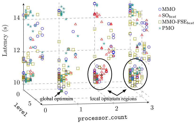
(b) LRZIP-O1

Figure 9: Projected landscapes of the explored configurations for two exampled systems. Each point is a configuration measured in the run, regardless whether it is preserved or not. (a) represents a case where MMO finds the global optimum while the others did not; (b) showcases the scenario where none of them found the global optimum, but MMO produces results that are much closer than those of the others.

5.2 RQ2: Resource Efficiency

5.2.1 Method

To understand the resource efficiency of MMO in RQ2, for each case out of the 22, we use the following procedure:

1. Identify a baseline, $b$, taken as the smallest number of measurements that the best single-objective counterpart (SO_best) consumes to achieve its best result of the target performance objective (says $T$), averaging over 50 runs.

2. For each of the MMO, MMO-FSE_best, and PMO, find the smallest number of measurements, denoted as $m$, at which the average result of the target performance objective (over 50 runs) is equivalent to or better than $T$.

3. The speedup over SO_best, i.e., $s={b\over m}$, is reported, according to the metric used by Gao et al. [33].

The greater the $s$, the better speedup, and hence more resources can be saved against that consumed by SO_best. In particular, if the MMO is resource-efficient, then we would expect at least $s=1$ and ideally $s>1$. Since in our context the resource is the number of measurements, it reflects the time and computation required by a model. Again, we consider the SO_best and MMO-FSE_best as identified for RQ1.

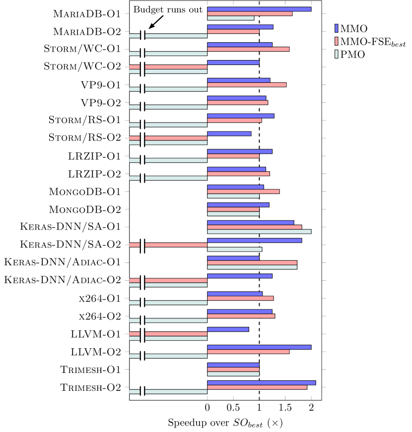
Figure 10: Speedup (denoted as $s$) for MMO, MMO-FSE with the best weight (MMO_best), and the PMO for converging to the best value (the average over 50 runs) of performance objective, $T$, by the best single-objective counterpart (SO_best), using its budget consumption as the baseline (the dashed line at speedup $1\times$). $0<s<1$ indicating that the method is even slower (by using more measurements) than SO_best to reach its best result, suggesting an inefficient utilization of resources. The broken bars mean $T$ has not been reached when the search budget runs out, i.e., $s<0$.

5.2.2 Findings

As can be seen from Figure 10, despite a very small number of cases where the MMO uses more resources to reach the performance level as achieved by the best single-objective counterpart, most commonly it uses less number of measurements than, or at least identical to, the baseline to find the same or better results, e.g., it obtains a speedup up to $2.09\times$. In particular, the MMO achieves 17 cases of $s>1$; 3 cases of $s=1$; and 2 cases of $0<s<1$. Remarkably, there is no case where it fails to reach the performance level when the budget runs out (the divided bars, denoted as $s<0$). This indicates that the MMO overcomes local optima better and more efficiently — a key attraction to software configuration tuning due to its expensive measurements. The MMO-FSE_best does show competitive results with respect to MMO: it has 13 cases of $s>1$ and 4 cases of $s=1$, but there are 5 cases of $s<0$ due to the issues discussed in Section 3.5, which could be undesirable on certain domains.

In contrast, the PMO exhibits the worst resource efficiency in terms of the speedup over $SO_{best}$, as it has 3 cases of $s>1$, together with 3 cases of $s=1$; 1 case of $0<s<1$, respectively, while the remaining 16 cases are $s<0$. This is a clear sign that PMO is generally resource-hungry as discussed in Section 3.

As the conclusion for RQ2, we say:

5.3 RQ3: Benefits over MMO-FSE

5.3.1 Method

In RQ3, we seek to confirm the benefits provided by the parameter-free design in MMO are indeed meaningful over MMO-FSE. Particularly, on each of the 22 systems/environments, we examine how does MMO performs against the MMO-FSE under different weights using the full-scale experiment. Indeed, if the differences between MMO and MMO-FSE over different weights are small, then perhaps using the MMO-FSE can be sufficient. Since we considered eight weights, there will be $8\times 22=176$ cases of comparisons. Again, the statistical test (i.e., the non-paired Wilcoxon rank-sum test) and effect size are reported for all each of those comparisons over 50 runs.

The other aspect we are interested in is how much extra resource would be required in order to identify the best weight when using MMO-FSE. This makes sense as if the effort to find the best weight in MMO-FSE is trivial, then one would merely need to find such weight in a case-by-case manner. To investigate such, we use the following procedure in each of the 22 systems/environments:

1. Run MMO-FSE under all weights studied with an incremental search budget that is proportional to that of the full-scale experiment, i.e., 10%, 20%, $...$, 100%. The experiment under each proportion of the budget is repeated 50 runs.

2. Find the smallest proportion of search budget, $p$, which discovers the same best weight as that identified under the full-scale experiment (with Scott-Knott test and mean over 50 runs).

3. The $p$ is then reported.

TABLE IV: $\hat{A}_{12}$ ($p$ value) on comparing MMO with MMO-FSE under different weights ($w$) over 50 runs. The blue cells denote the cases where MMO wins while red cells denote those that it loses; otherwise it is a tie. The statistically significant comparisons, i.e., $\hat{A}_{12}\geq 0.56$ (or $\hat{A}_{12}\leq 0.44$) and $p<0.05$ are highlighted in bold.

Software System	$w=0.01$	$w=0.1$	$w=0.3$	$w=0.5$	$w=0.7$	$w=0.9$	$w=1$	$w=10$
MariaDB-O1	.60 ($=$.102)	.56 ($=$.287)	.43 ($=$.197)	.54 ($=$.533)	.49 ($=$.882)	.58 ($=$.178)	.52 ($=$.717)	.96 ($<$.001)
MariaDB-O2	.53 ($=$.608)	.60 ($=$.079)	.64 ($=$.019)	.66 ($=$.007)	.65 ($=$.010)	.69 ($<$.001)	.70 ($<$.001)	.75 ($<$.001)
Storm/WC-O1	.57 ($=$.212)	.55 ($=$.356)	.60 ($=$.071)	.61 ($=$.062)	.48 ($=$.746)	.46 ($=$.491)	.49 ($=$.879)	.65 ($=$.012)
Storm/WC-O2	.99 ($<$.001)	1.0 ($<$.001)	.99 ($<$.001)	1.0 ($<$.001)	1.0 ($<$.001)	1.0 ($<$.001)	1.0 ($<$.001)	1.0 ($<$.001)
VP9-O1	.57 ($=$.197)	.44 ($=$.279)	.55 ($=$.402)	.62 ($=$.043)	.74 ($<$.001)	.84 ($<$.001)	.86 ($<$.001)	.93 ($<$.001)
VP9-O2	.55 ($=$.396)	.48 ($=$.754)	.64 ($=$.016)	.71 ($<$.001)	.65 ($=$.009)	.73 ($<$.001)	.65 ($=$.011)	.91 ($<$.001)
Storm/RS-O1	.53 ($=$.605)	.54 ($=$.491)	.56 ($=$.301)	.55 ($=$.389)	.55 ($=$.389)	.54 ($=$.491)	.52 ($=$.720)	.73 ($<$.001)
Storm/RS-O2	.94 ($<$.001)	1.0 ($<$.001)	1.0 ($<$.001)	1.0 ($<$.001)	1.0 ($<$.001)	1.0 ($<$.001)	1.0 ($<$.001)	1.0 ($<$.001)
LRZIP-O1	.77 ($<$.001)	.97 ($<$.001)	.98 ($<$.001)	.99 ($<$.001)	.98 ($<$.001)	.98 ($<$.001)	.98 ($<$.001)	.99 ($<$.001)
LRZIP-O2	.51 ($=$.820)	.55 ($=$.363)	.77 ($<$.001)	.84 ($<$.001)	.84 ($<$.001)	.84 ($<$.001)	.85 ($<$.001)	.90 ($<$.001)
MongoDB-O1	.54 ($=$.535)	.63 ($=$.022)	.62 ($=$.034)	.65 ($=$.010)	.65 ($=$.011)	.59 ($=$.105)	.65 ($=$.010)	.76 ($<$.001)
MongoDB-O2	.62 ($=$.034)	.58 ($=$.196)	.64 ($=$.016)	.63 ($=$.029)	.64 ($=$.018)	.65 ($=$.012)	.67 ($=$.003)	.67 ($=$.003)
Keras-DNN/SA-O1	.58 ($=$.166)	.55 ($=$.387)	.54 ($=$.493)	.73 ($<$.001)	.72 ($<$.001)	.69 ($=$.001)	.74 ($<$.001)	.75 ($<$.001)
Keras-DNN/SA-O2	.94 ($<$.001)	.99 ($<$.001)	1.0 ($<$.001)	.98 ($<$.001)	.99 ($<$.001)	.96 ($<$.001)	.99 ($<$.001)	1.0 ($<$.001)
Keras-DNN/Adiac-O1	.67 ($=$.004)	.54 ($=$.517)	.66 ($=$.004)	.64 ($=$.014)	.68 ($=$.002)	.62 ($=$.033)	.70 ($<$.001)	.71 ($<$.001)
Keras-DNN/Adiac-O2	.99 ($<$.001)	1.0 ($<$.001)	1.0 ($<$.001)	1.0 ($<$.001)	1.0 ($<$.001)	1.0 ($<$.001)	1.0 ($<$.001)	1.0 ($<$.001)
x264-O1	.48 ($=$.738)	.44 ($=$.324)	.48 ($=$.674)	.56 ($=$.334)	.59 ($=$.119)	.45 ($=$.370)	.54 ($=$.540)	.59 ($=$.129)
x264-O2	.65 ($=$.009)	.59 ($=$.143)	.59 ($=$.120)	.57 ($=$.247)	.50 ($=$.956)	.57 ($=$.255)	.52 ($=$.762)	.58 ($=$.190)
LLVM-O1	.50 ($=$1.00)	.50 ($=$1.00)	.50 ($=$1.00)	.50 ($=$1.00)	.50 ($=$1.00)	.50 ($=$1.00)	.50 ($=$1.00)	.80 ($<$.001)
LLVM-O2	.61 ($=$.062)	.59 ($=$.107)	.62 ($=$.036)	.63 ($=$.020)	.59 ($=$.127)	.59 ($=$.124)	.64 ($=$.019)	.59 ($=$.137)
Trimesh-O1	.50 ($=$1.00)	.50 ($=$1.00)	.50 ($=$1.00)	.50 ($=$1.00)	.50 ($=$1.00)	.50 ($=$1.00)	.50 ($=$1.00)	.50 ($=$1.00)
Trimesh-O2	.58 ($=$.186)	.52 ($=$.672)	.85 ($<$.001)	.90 ($<$.001)	.93 ($<$.001)	.94 ($<$.001)	.92 ($<$.001)	.91 ($<$.001)

[width=0.8]figures/find-weight

Figure 11: The necessary resource consumed $p$ (in terms of % on the full-scale experiments’ search budget) for the MMO-FSE to find the same best weight as that identified under the full-scale experiments; these are the resource that would have been saved by using MMO. As a reference, the dashed line highlights the 50% threshold of the budget. All cases are sorted in descending order.

5.3.2 Findings

As we can see from Table IV, the MMO-FSE is highly sensitive to its weight setting, as often there is only one (or two) best weight that can significantly outperform the others (e.g., MariaDB-O1 and VP9-O1) and the best $w$ differs significantly across systems, suggesting that it is meaningful for having the parameter-free property enabled by the new normalization in MMO. In particular, the MMO wins 149 out of the 175 cases (103 with statistical significance), loses on 11, and with 15 ties. As shown in Sections 5.1 and 5.2, even when compared with the MMO-FSE under the best weight, the MMO remains very competitive and doing so without the need for weight tuning.

To understand how much extra resource is required to tune the weight in MMO-FSE, Figure 11 illustrates the results. Clearly, we see that for 14 out of the 22 cases, it needs 50% or more of the full-scale search budget to identify the best weight, which may not be acceptable when using the MMO-FSE under a case; or otherwise, the quality of tuning could be compromised. Even for the 8 cases where the extra resource required are between 10% and 30%, it may still be undesirable since some systems, such as VP9, can take up to 190 seconds to measure a single configuration.

Therefore, for RQ3, we say:

TABLE V: Comparing Flash${}_{\textsc{MMO}}$ and Flash over 50 runs. The format is the same as Table III.

max width = 1

Mean/SE $\hat{A}_{12}$ ($p$ value) Flash max width=.1 .62 ($<$.001) Flash${}_{\textsc{MMO}}$ max width=.1 -		Mean/SE $\hat{A}_{12}$ ($p$ value) max width=.1 .48 ($=$.101) max width=.1 -		Mean/SE $\hat{A}_{12}$ ($p$ value) max width=.1 .33 ($<$.001) max width=.1 -		Mean/SE $\hat{A}_{12}$ ($p$ value) max width=.1 .53 ($<$.001) max width=.1 -
(a). MariaDB-O1		(b). MariaDB-O2		(c). Storm/WC-O1		(d). Storm/WC-O2
Mean/SE $\hat{A}_{12}$ ($p$ value) Flash max width=.1 .49 ($=$.530) Flash${}_{\textsc{MMO}}$ max width=.1 -		Mean/SE $\hat{A}_{12}$ ($p$ value) max width=.1 .91 ($<$.001) max width=.1 -		Mean/SE $\hat{A}_{12}$ ($p$ value) max width=.1 .31 ($<$.001) max width=.1 -		Mean/SE $\hat{A}_{12}$ ($p$ value) max width=.1 .56 ($=$.040) max width=.1 -
(e). VP9-O1		(f). VP9-O2		(g). Storm/RS-O1		(h). Storm/RS-O2
Mean/SE $\hat{A}_{12}$ ($p$ value) Flash max width=.1 .58 ($=$.044) Flash${}_{\textsc{MMO}}$ max width=.1 -		Mean/SE $\hat{A}_{12}$ ($p$ value) max width=.1 .58 ($=$.015) max width=.1 -		Mean/SE $\hat{A}_{12}$ ($p$ value) max width=.1 .67 ($=$.008) max width=.1 -		Mean/SE $\hat{A}_{12}$ ($p$ value) max width=.1 .73 ($<$.001) max width=.1 -
(i). LRZIP-O1		(j). LRZIP-O2		(k). MongoDB-O1		(l). MongoDB-O2
Mean/SE $\hat{A}_{12}$ ($p$ value) Flash max width=.1 .63 ($=$.011) Flash${}_{\textsc{MMO}}$ max width=.1 -		Mean/SE $\hat{A}_{12}$ ($p$ value) max width=.1 .78 ($<$.001) max width=.1 -		Mean/SE $\hat{A}_{12}$ ($p$ value) max width=.1 .61 ($=$.005) max width=.1 -		Mean/SE $\hat{A}_{12}$ ($p$ value) max width=.1 .67 ($=$.002) max width=.1 -
(n). Keras-DNN/SA-O1		(m). Keras-DNN/SA-O2		(o). Keras-DNN/Adiac-O1		(p). Keras-DNN/Adiac-O2
Mean/SE $\hat{A}_{12}$ ($p$ value) Flash max width=.1 .26 ($<$.001) Flash${}_{\textsc{MMO}}$ max width=.1 -		Mean/SE $\hat{A}_{12}$ ($p$ value) max width=.1 .36 ($<$.001) max width=.1 -		Mean/SE $\hat{A}_{12}$ ($p$ value) max width=.1 .78 ($<$.001) max width=.1 -		Mean/SE $\hat{A}_{12}$ ($p$ value) max width=.1 .47 ($<$.001) max width=.1 -
(q). x264-O1		(r). x264-O2		(s). LLVM-O1		(t). LLVM-O2
Mean/SE $\hat{A}_{12}$ ($p$ value) Flash max width=.1 .51 ($<$.001) Flash${}_{\textsc{MMO}}$ max width=.1 -		Mean/SE $\hat{A}_{12}$ ($p$ value) max width=.1 .54 ($=$.103) max width=.1 -	% Win % Lose % Tie Flash${}_{\textsc{MMO}}$ vs. Flash 68% 32% 0%
(u). Trimesh-O1		(v). Trimesh-O2	(w). Overall % win/loss/tie for Flash${}_{\textsc{MMO}}$ versus Flash

5.4 RQ4: Consolidating Model-based Tuning

5.4.1 Method

For RQ4, we extended Flash with our MMO, denoted as Flash${}_{\textsc{MMO}}$. As shown in Algorithm 3, the change is highlighted in colors, from which we see that the amendment is merely a single line of code which changes the random search that solely optimizes the target performance objective to searching over the space of MMO (working with NSGA-II). In this way, the search is conducted in the transformed meta bi-objective space of the surrogate-predicted objectives, in which the system $\mathcal{F}$ is replaced by the surrogates $\mathcal{M}$. For both Flash and Flash${}_{\textsc{MMO}}$, we allow 1,000 evaluations, including redundant ones, on the surrogate (50 population size and 20 generations in Flash${}_{\textsc{MMO}}$) as from existing work [9, 45, 65].

Similar to the previous sections, the statistical test and effect size are reported for every pairwise comparison between the Flash${}_{\textsc{MMO}}$ and Flash over 50 runs.

1

Input: Configuration space $\mathcal{V}$; the system $\mathcal{F}$

2

Output: ${s}_{best}$ the best configuration on $f_{t}(\boldsymbol{x})$

Declare: vector of surrogates $\mathcal{M}$ (one for each performance objective)

3 Randomly initialize a size of $k$ configurations $\mathcal{P}$

4 measure($\mathcal{P},\mathcal{F}$)

5 $\mathcal{V}\leftarrow$$\mathcal{V}-\mathcal{P}$

6 while The search budget is not exhausted do

7       $\mathcal{M}=$ CARTs($\mathcal{P}$)

8       /* searching an estimated-best configuration in the transformed meta bi-objective space defined by the MMO (with NSGA-II), as shown in Algorithm 1 */

9       ${o}=$ search($\mathcal{V},\mathcal{M}$)

10       ${o}=$ MMOonNSGA-II($\mathcal{V},\mathcal{M}$)

11       measure(${o},\mathcal{F}$)

12       $\mathcal{V}\leftarrow$$\mathcal{V}-{o}$

13       $\mathcal{P}\leftarrow$$\mathcal{P}+{o}$

14       if ${o}$ is measured to be better than ${s}_{best}$ on $f_{t}(\boldsymbol{x})$ then

15             ${s}_{best}={o}$

16            

17      

18

19return ${s}_{best}$

Algorithm 3 Flash${}_{\textsc{MMO}}$

5.4.2 Findings

From Table V, it is clear that Flash${}_{\textsc{MMO}}$ obtains better results than Flash in general: it wins 15 out of 22 cases while lose 7 others. In particular, in those cases where Flash${}_{\textsc{MMO}}$ wins, 12 of them are statistically significant. In contrast, only 4 of those that it loses have $p<0.05$ and non-trivial effect size. The relative magnitude of gains have also been significant, e.g., for VP9-O2 and Storm/RS-O2. This means that, even when searching within the surrogate-predicted space, our MMO can bring considerable improvement on model-based tuning methods like Flash.

To take a closer investigation, Figure 12 shows the overall search trajectories for the 20 measurements that are actually spent on tuning. Clearly, Flash${}_{\textsc{MMO}}$ produces a trajectory with a steeper slope than that of Flash over all cases and runs. The standard error of the average performance is also smaller, implying that MMO can also consolidate the stability of outcomes. Of particular interesting points are at the 32th and 41st sample of measurements: the former means that Flash${}_{\textsc{MMO}}$ improves the results at as little as the 2nd sample into the tuning (as the first 30 are for pre-training the surrogate); while the latter reflects that the MMO helps to improve resource efficiency, achieving a ${50\over 41}=1.22\times$ speedup over Flash when reaching its best outcome under the search budget.

Overall, for RQ5, we have:

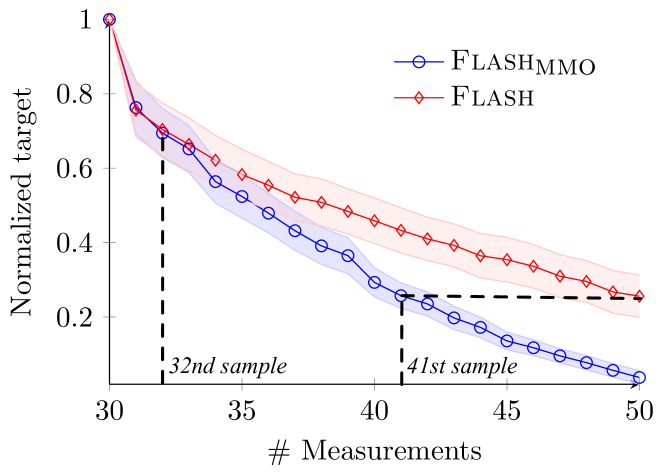
Figure 12: The search trajectories for Flash${}_{\textsc{MMO}}$ and Flash. Each point shows the average and the corresponding standard error over all cases and 50 runs. The target performance objectives are normalized and converted as minimizing objectives, if needed; hence the smaller, the better.

6 Threats to Validity

Threats to internal validity can be related to the search budget. To tackle this, we have set the budget that reaches a reasonable convergence for all the optimizers compared — a typical setup when the study aims to examine the effectiveness of mitigating local optima [63]. The other parameter settings follow what has been pragmatically used from the literature [25, 69, 28, 9, 45, 65]. or tuned through preliminary runs. However, we acknowledge that examining alternative parameters can be an interesting topic and we leave this for future work. To mitigate bias, we repeated 50 experiment runs under each case.

The metrics and evaluation used may pose threats to construct validity. Since there is only a single performance concern, there is no need to consider metrics with respect to multi-objective optimization [54, 53]. We conduct the comparison based on the target performance objective and to the resource (number of measurements) required to converge to the same result. Both of these are common metrics in software configuration tuning [60, 33]. To verify statistical significance and effect size, we use the Wilcoxon test (including both the paired and non-paired versions depending on the research questions) and $\hat{A}_{12}$ to examine the results. While the MMO model is optimizer-agnostic, we examine mainly on NSGA-II in this work; using alternative multi-objective optimizers is unlikely to invalidate our conclusion but we admit the usefulness of evaluating over a wide range of optimizers with MMO, which can be part of the future work.

Threats to external validity can be raised from the subjects studied. We mitigated this by using 11 systems/environments that are of different domains, scales, and performance attributes, as used by prior work [60, 43, 57, 44, 64]. We also compared the proposed MMO (under the new normalization) with four state-of-the-art single-objective counterparts for software configuration tuning, PMO model, and the MMO-FSE. Further, we examine how it can help to consolidate Flash, a recent model-based tuning method from the software engineering community. Nonetheless, we agree that studying additional systems and optimizers may prove fruitful.

7 Related Work

Broadly, optimizers for software configuration tuning can be either measurement-based or model-based.

7.1 Measurement-based Tuning

In measurement-based tuning methods, the optimizer is guided by directly measuring the configuration on the software systems. Despite the expensiveness, the measurements can accurately reflect the good or bad of a configuration (and the extents thereof). A wide range of optimizers have been studied, such as random search [7, 87, 61, 67], hill climbing [83, 52, 31], single-objective genetic algorithm [6, 69, 73] and simulated annealing [34, 35], to name a few.

Under such a single-objective model, a key difference for those optimizers lies in the tricks that attempt to overcome the issues of local optima. For example, some extend the random search to consider a wider neighboring radius of the configuration structure, hence it is more likely to jump out from the local optima [61]. Others rely on restarting from a different point, such as in restarted hill climbing, hence increasing the chance to find the “right” path from local optima to the global optimum [90, 83]. More recently, Krishna et al. [47] has relied on probabilistically accepting worse configurations to jump out of local optima — a typical feature of the simulated annealing [31, 35].

Our MMO differs from all the above as it lies in a higher level of abstraction — the optimization model — as opposed to the level of optimization method. In particular, with the new normalization, the purposely-crafted Pareto relation in MMO has been shown to be able to better overcome the local optima for software configuration tuning.

7.2 Model-based Tuning

Instead of solely using the measurements of software systems, the model-based tuning methods apply a surrogate (analytical [49, 27, 28] or machine learning based [60, 43]) to evaluate configurations, which guides the search in an optimizer. The intention is to speed up the exploration of configurations as the model evaluation is much cheaper. Yet, it has been shown that the model accuracy and the availability of initial data can become an issue [90].

Studies on model-based tuning for software systems differ mainly on the way of building surrogate and the choice of acquisition function. Among others, Jamshidi and Casale [43] use Bayesian optimization to tune software configuration, wherein the search is guided by the Gaussian Process based surrogate trained from the data collected. Nair et al. [60] follow a similar idea to propose Flash, but the CART is used instead as the surrogate. More recently, Chen et al. [16] also follow BO and CART but they additionally identify the “important configuration options” from the Random Forest model. Such information would then inform the optimization of the acquisition function in determining what to sample next.

Since MMO lies in the level of optimization model, it is complementary to the model-based methods in which the MMO would take the surrogate values as inputs instead of the real measurements. This, as we have shown using Flash as a case, can better consolidate the tuning results.

7.3 General Parameter Tuning

Optimizers proposed for the parameter tuning of general algorithms can also be relevant [11, 39, 8, 66], including IRace [55], ParamILS [41], SMAC [40], GGA$++$ [4], as well as their multi-objective variants, such as MO-ParamILS [10] and SPRINT-Race [89]. To examine a few examples, ParamILS [41] relies on iterative local search — a search procedure that may jump out of local optima using strategies similar to that of SA and SHC-r. Further, a key contribution is the capping strategy, which helps to reduce the need to measure an algorithm under some problem instances, hence saving computational resources. This is one of the goals that we seek to achieve too. Similar to Nair et al. [60], SMAC [40] uses Bayesian optimization but relies on a Random Forest model, which additionally considers the performance of an algorithm over a set of instances.

However, their work differs from ours in two aspects. Firstly, general algorithm configuration requires working on a set of problem instances, each coming with different features. The software configuration tuning, in contrast, is often concerned with tuning software systems under a given benchmark (i.e., one instance) [60, 43, 90, 25]. Therefore, most of their designs for saving resources (such as the capping in ParamILS) were proposed to reduce the number of instances measured. Of course, it is possible to generalize the problem to consider multiple benchmarks at the same time, yet this is outside the scope of this paper. Secondly, none of them works on the level of optimization model, and therefore, similar to the case of Flash, our MMO is still complementary to their optimizers.

7.4 Multi-objectivization in SBSE

Multi-objectivization, which is the notion behind our MMO model, has been applied in other SBSE problems [88, 30, 58, 75]. For example, to reproduce a crash based on the crash report, one can purposely design a new auxiliary objective, which measures how widely a test case covers the code, to be optimized alongside with the target crash distance [30]. A multi-objective optimizer, e.g., NSGA-II, is directly used thereafter. A similar case can be found also for the code refactoring problem [58]. However, during the tuning process, such a model, i.e., PMO in this paper, can result in poor resource efficiency as it wastes a significant amount of the resource in optimizing the auxiliary objective, which is of no interest. This is a particularly unwelcome issue for software configuration tuning where the measurement is expensive. As we have shown in Section 5, PMO performs even worse than the classic single-objective model in most of the cases.

8 Conclusion and Future Work

To mitigate the local optima issue in software configuration tuning, this paper takes a different perspective — multi-objectivizing the single objective optimization scenario. We do this by proposing a meta multi-objective model (MMO), at the level of optimization model (external part), as opposed to existing work that focuses on developing an effective single-objective optimizer (internal part). This work also overcomes an important limitation from our prior FSE work, namely eliminating the need for the weight parameter in the MMO model, while achieving even better results.

We compare MMO under the new normalization with four state-of-the-art single-objective optimizers, the plain multi-objectivization model, and the MMO model with the old normalization from our prior FSE work over 22 cases that are of diverse performance attributes, systems, and environments. The results reveal that the MMO model:

• can generally be more effective in overcoming local optima with better results;

• and does so by utilizing resources more efficiently (better speedup) in most cases;

• saves a considerable amount of extra resource that would otherwise be required for identifying the best weight.

Furthermore, we use MMO as part of Flash, a recent effort from the software engineering community for configuration tuning, and revealing that it can:

• considerably consolidate the results;

• while enabling good speedup overall.

Future directions of this work are exciting and fruitful, as it paves a new way of thinking about the resolution for mitigating local optima in software configuration and perhaps in a wider context of SBSE — multi-objectivizing at the level of optimization model instead of working at the level of an optimizer/algorithm. Specifically, the most immediate next steps include extending MMO beyond two meta-objectives (e.g., through considering multiple auxiliary objectives if any) and exploring the possibility to design tailored multi-objectivization model for other SBSE problems.

Appendix A

Remark 1.

The global optimum of the original single-objective problem is Pareto optimal in MMO.

Proof.

(By contradiction) Let the global optimum of the original single-objective problem be $\boldsymbol{p}$. Then, $\forall\boldsymbol{x}\in\mathbfcal{X},f_{t}(\boldsymbol{p})\leq f_{t}(\boldsymbol{x})$. Assuming that $\boldsymbol{p}$ is not a Pareto optimal solution for the MMO model of Equation 3, then there exists at least one solution $\boldsymbol{q}$ such that $\boldsymbol{q}\prec\boldsymbol{p}$. That is

$$\begin{split}\begin{cases}f_{t}(\boldsymbol{q})+wf_{a}(\boldsymbol{q})<f_{t}(\boldsymbol{p})+wf_{a}(\boldsymbol{p})\\ f_{t}(\boldsymbol{q})-wf_{a}(\boldsymbol{q})\leq f_{t}(\boldsymbol{p})-wf_{a}(\boldsymbol{p})\\ \end{cases}\end{split}$$

or

$$\begin{split}\begin{cases}f_{t}(\boldsymbol{q})+wf_{a}(\boldsymbol{q})\leq f_{t}(\boldsymbol{p})+wf_{a}(\boldsymbol{p})\\ f_{t}(\boldsymbol{q})-wf_{a}(\boldsymbol{q})<f_{t}(\boldsymbol{p})-wf_{a}(\boldsymbol{p})\\ \end{cases}\end{split}$$

For either of the above equations, adding up the left and right sides of the two parts, respectively, we have $2f_{t}(\boldsymbol{q})<2f_{t}(\boldsymbol{p})$, a contradiction to $\boldsymbol{p}$ being the global optimum of the problem. ∎

References

- [1] R. B. Abdessalem, A. Panichella, S. Nejati, L. C. Briand, and T. Stifter, “Automated repair of feature interaction failures in automated driving systems,” in ISSTA ’20: 29th ACM SIGSOFT International Symposium on Software Testing and Analysis, Virtual Event, USA, July 18-22, 2020, S. Khurshid and C. S. Pasareanu, Eds. ACM, 2020, pp. 88–100. [Online]. Available: https://doi.org/10.1145/3395363.3397386
- [2] M. A. Ahmad, C. Eckert, and A. Teredesai, “Interpretable machine learning in healthcare,” in Proceedings of the 2018 ACM International Conference on Bioinformatics, Computational Biology, and Health Informatics, BCB 2018, Washington, DC, USA, August 29 - September 01, 2018, A. Shehu, C. H. Wu, C. Boucher, J. Li, H. Liu, and M. Pop, Eds. ACM, 2018, pp. 559–560. [Online]. Available: https://doi.org/10.1145/3233547.3233667
- [3] M. Alrifai, T. Risse, P. Dolog, and W. Nejdl, “A scalable approach for qos-based web service selection,” in Service-Oriented Computing - ICSOC 2008 Workshops, ICSOC 2008 International Workshops, Sydney, Australia, December 1st, 2008, Revised Selected Papers, ser. Lecture Notes in Computer Science, G. Feuerlicht and W. Lamersdorf, Eds., vol. 5472. Springer, 2008, pp. 190–199. [Online]. Available: https://doi.org/10.1007/978-3-642-01247-1_20
- [4] C. Ansótegui, Y. Malitsky, H. Samulowitz, M. Sellmann, and K. Tierney, “Model-based genetic algorithms for algorithm configuration,” in Proceedings of the Twenty-Fourth International Joint Conference on Artificial Intelligence, IJCAI 2015, Buenos Aires, Argentina, July 25-31, 2015, Q. Yang and M. J. Wooldridge, Eds. AAAI Press, 2015, pp. 733–739. [Online]. Available: http://ijcai.org/Abstract/15/109
- [5] A. Arcuri and L. C. Briand, “A practical guide for using statistical tests to assess randomized algorithms in software engineering,” in ICSE’11: Proc. of the 33rd International Conference on Software Engineering. ACM, 2011, pp. 1–10.
- [6] B. Behzad, H. V. T. Luu, J. Huchette, S. Byna, Prabhat, R. A. Aydt, Q. Koziol, and M. Snir, “Taming parallel I/O complexity with auto-tuning,” in International Conference for High Performance Computing, Networking, Storage and Analysis, SC’13, Denver, CO, USA - November 17 - 21, 2013, W. Gropp and S. Matsuoka, Eds. ACM, 2013, pp. 68:1–68:12. [Online]. Available: https://doi.org/10.1145/2503210.2503278
- [7] J. Bergstra and Y. Bengio, “Random search for hyper-parameter optimization,” J. Mach. Learn. Res., vol. 13, pp. 281–305, 2012. [Online]. Available: http://dl.acm.org/citation.cfm?id=2188395
- [8] L. C. T. Bezerra, M. López-Ibáñez, and T. Stützle, “Automatic configuration of multi-objective optimizers and multi-objective configuration,” in High-Performance Simulation-Based Optimization, ser. Studies in Computational Intelligence, T. Bartz-Beielstein, B. Filipic, P. Korosec, and E. Talbi, Eds. Springer, 2020, vol. 833, pp. 69–92. [Online]. Available: https://doi.org/10.1007/978-3-030-18764-4_4
- [9] Z. Bingul, “Adaptive genetic algorithms applied to dynamic multiobjective problems,” Appl. Soft Comput., vol. 7, no. 3, pp. 791–799, 2007. [Online]. Available: https://doi.org/10.1016/j.asoc.2006.03.001
- [10] A. Blot, H. H. Hoos, L. Jourdan, M. Kessaci-Marmion, and H. Trautmann, “Mo-paramils: A multi-objective automatic algorithm configuration framework,” in Learning and Intelligent Optimization - 10th International Conference, LION 10, Ischia, Italy, May 29 - June 1, 2016, Revised Selected Papers, ser. Lecture Notes in Computer Science, P. Festa, M. Sellmann, and J. Vanschoren, Eds., vol. 10079. Springer, 2016, pp. 32–47. [Online]. Available: https://doi.org/10.1007/978-3-319-50349-3_3
- [11] A. Blot, M. Marmion, L. Jourdan, and H. H. Hoos, “Automatic configuration of multi-objective local search algorithms for permutation problems,” Evol. Comput., vol. 27, no. 1, pp. 147–171, 2019. [Online]. Available: https://doi.org/10.1162/evco_a_00240
- [12] L. Breiman, J. H. Friedman, R. A. Olshen, and C. J. Stone, Classification and Regression Trees. Wadsworth, 1984.
- [13] T. B. Brown, B. Mann, N. Ryder, M. Subbiah, J. Kaplan, P. Dhariwal, A. Neelakantan, P. Shyam, G. Sastry, A. Askell et al., “Language models are few-shot learners,” arXiv preprint arXiv:2005.14165, 2020.
- [14] A. Buzdalova, M. Buzdalov, and V. Parfenov, “Generation of tests for programming challenge tasks using helper-objectives,” in Search Based Software Engineering - 5th International Symposium, SSBSE 2013, St. Petersburg, Russia, August 24-26, 2013. Proceedings, ser. Lecture Notes in Computer Science, G. Ruhe and Y. Zhang, Eds., vol. 8084. Springer, 2013, pp. 300–305. [Online]. Available: https://doi.org/10.1007/978-3-642-39742-4_28
- [15] Z. Cai and Y. Wang, “A multiobjective optimization-based evolutionary algorithm for constrained optimization,” IEEE Transactions on evolutionary computation, vol. 10, no. 6, pp. 658–675, 2006.
- [16] J. Chen, N. Xu, P. Chen, and H. Zhang, “Efficient compiler autotuning via bayesian optimization,” in 43rd IEEE/ACM International Conference on Software Engineering, ICSE 2021, Madrid, Spain, 22-30 May 2021. IEEE, 2021, pp. 1198–1209. [Online]. Available: https://doi.org/10.1109/ICSE43902.2021.00110
- [17] T. Chen, “All versus one: an empirical comparison on retrained and incremental machine learning for modeling performance of adaptable software,” in Proceedings of the 14th International Symposium on Software Engineering for Adaptive and Self-Managing Systems, SEAMS@ICSE 2019, Montreal, QC, Canada, May 25-31, 2019, M. Litoiu, S. Clarke, and K. Tei, Eds. ACM, 2019, pp. 157–168. [Online]. Available: https://doi.org/10.1109/SEAMS.2019.00029
- [18] T. Chen and R. Bahsoon, “Self-adaptive and sensitivity-aware qos modeling for the cloud,” in Proceedings of the 8th International Symposium on Software Engineering for Adaptive and Self-Managing Systems, SEAMS 2013, San Francisco, CA, USA, May 20-21, 2013, M. Litoiu and J. Mylopoulos, Eds. IEEE Computer Society, 2013, pp. 43–52. [Online]. Available: https://doi.org/10.1109/SEAMS.2013.6595491
- [19] ——, “Self-adaptive and online qos modeling for cloud-based software services,” IEEE Trans. Software Eng., vol. 43, no. 5, pp. 453–475, 2017. [Online]. Available: https://doi.org/10.1109/TSE.2016.2608826
- [20] ——, “Self-adaptive trade-off decision making for autoscaling cloud-based services,” IEEE Trans. Serv. Comput., vol. 10, no. 4, pp. 618–632, 2017. [Online]. Available: https://doi.org/10.1109/TSC.2015.2499770
- [21] T. Chen, R. Bahsoon, S. Wang, and X. Yao, “To adapt or not to adapt?: Technical debt and learning driven self-adaptation for managing runtime performance,” in Proceedings of the 2018 ACM/SPEC International Conference on Performance Engineering, ICPE 2018, Berlin, Germany, April 09-13, 2018, K. Wolter, W. J. Knottenbelt, A. van Hoorn, and M. Nambiar, Eds. ACM, 2018, pp. 48–55. [Online]. Available: https://doi.org/10.1145/3184407.3184413
- [22] T. Chen, R. Bahsoon, and X. Yao, “Online qos modeling in the cloud: A hybrid and adaptive multi-learners approach,” in Proceedings of the 7th IEEE/ACM International Conference on Utility and Cloud Computing, UCC 2014, London, United Kingdom, December 8-11, 2014. IEEE Computer Society, 2014, pp. 327–336. [Online]. Available: https://doi.org/10.1109/UCC.2014.42
- [23] ——, “A survey and taxonomy of self-aware and self-adaptive cloud autoscaling systems,” ACM Comput. Surv., vol. 51, no. 3, pp. 61:1–61:40, 2018. [Online]. Available: https://doi.org/10.1145/3190507
- [24] ——, “Synergizing domain expertise with self-awareness in software systems: A patternized architecture guideline,” Proc. IEEE, vol. 108, no. 7, pp. 1094–1126, 2020. [Online]. Available: https://doi.org/10.1109/JPROC.2020.2985293
- [25] T. Chen, K. Li, R. Bahsoon, and X. Yao, “FEMOSAA: Feature guided and knee driven multi-objective optimization for self-adaptive software,” ACM Transactions on Software Engineering and Methodology, vol. 27, no. 2, 2018.
- [26] T. Chen and M. Li, “Multi-objectivizing software configuration tuning,” in ESEC/FSE ’21: 29th ACM Joint European Software Engineering Conference and Symposium on the Foundations of Software Engineering, Athens, Greece, August 23-28, 2021, D. Spinellis, G. Gousios, M. Chechik, and M. D. Penta, Eds. ACM, 2021, pp. 453–465. [Online]. Available: https://doi.org/10.1145/3468264.3468555
- [27] T. Chen, M. Li, and X. Yao, “On the effects of seeding strategies: a case for search-based multi-objective service composition,” in Proceedings of the Genetic and Evolutionary Computation Conference, GECCO 2018, Kyoto, Japan, July 15-19, 2018, H. E. Aguirre and K. Takadama, Eds. ACM, 2018, pp. 1419–1426. [Online]. Available: https://doi.org/10.1145/3205455.3205513
- [28] ——, “Standing on the shoulders of giants: Seeding search-based multi-objective optimization with prior knowledge for software service composition,” Inf. Softw. Technol., vol. 114, pp. 155–175, 2019. [Online]. Available: https://doi.org/10.1016/j.infsof.2019.05.013
- [29] M. Cremene, M. A. Suciu, D. Pallez, and D. Dumitrescu, “Comparative analysis of multi-objective evolutionary algorithms for qos-aware web service composition,” Appl. Soft Comput., vol. 39, pp. 124–139, 2016. [Online]. Available: https://doi.org/10.1016/j.asoc.2015.11.012
- [30] P. Derakhshanfar, X. Devroey, A. Zaidman, A. van Deursen, and A. Panichella, “Good things come in threes: Improving search-based crash reproduction with helper objectives,” in 35th IEEE/ACM International Conference on Automated Software Engineering (ASE’20), 2020.
- [31] X. Ding, Y. Liu, and D. Qian, “Jellyfish: Online performance tuning with adaptive configuration and elastic container in hadoop yarn,” in 21st IEEE International Conference on Parallel and Distributed Systems, ICPADS 2015, Melbourne, Australia, December 14-17, 2015. IEEE Computer Society, 2015, pp. 831–836. [Online]. Available: https://doi.org/10.1109/ICPADS.2015.112
- [32] J. J. Durillo and A. J. Nebro, “jmetal: A java framework for multi-objective optimization,” Adv. Eng. Softw., vol. 42, no. 10, pp. 760–771, 2011. [Online]. Available: https://doi.org/10.1016/j.advengsoft.2011.05.014
- [33] Y. Gao, Y. Zhu, H. Zhang, H. Lin, and M. Yang, “Resource-guided configuration space reduction for deep learning models,” in 43rd IEEE/ACM International Conference on Software Engineering, ICSE 2021, Madrid, Spain, 22-30 May 2021. IEEE, 2021, pp. 175–187. [Online]. Available: https://doi.org/10.1109/ICSE43902.2021.00028
- [34] B. J. Garvin, M. B. Cohen, and M. B. Dwyer, “An improved meta-heuristic search for constrained interaction testing,” in 2009 1st International Symposium on Search Based Software Engineering. IEEE, 2009, pp. 13–22.
- [35] J. Guo, Q. Yi, and A. Qasem, “Evaluating the role of optimization-specific search heuristics in effective autotuning,” Technical report, 2010.
- [36] X. Han and T. Yu, “An empirical study on performance bugs for highly configurable software systems,” in Proceedings of the 10th ACM/IEEE International Symposium on Empirical Software Engineering and Measurement, ESEM 2016, Ciudad Real, Spain, September 8-9, 2016. ACM, 2016, pp. 23:1–23:10. [Online]. Available: https://doi.org/10.1145/2961111.2962602
- [37] R. M. Hierons, M. Li, X. Liu, J. A. Parejo, S. Segura, and X. Yao, “Many-objective test suite generation for software product lines,” ACM Transactions on Software Engineering and Methodology, vol. 29, no. 1, 2020.
- [38] R. M. Hierons, M. Li, X. Liu, S. Segura, and W. Zheng, “Sip: optimal product selection from feature models using many-objective evolutionary optimization,” ACM Transactions on Software Engineering and Methodology, vol. 25, no. 2, p. 17, 2016.
- [39] C. Huang, Y. Li, and X. Yao, “A survey of automatic parameter tuning methods for metaheuristics,” IEEE Trans. Evol. Comput., vol. 24, no. 2, pp. 201–216, 2020. [Online]. Available: https://doi.org/10.1109/TEVC.2019.2921598
- [40] F. Hutter, H. H. Hoos, and K. Leyton-Brown, “Sequential model-based optimization for general algorithm configuration,” in LION5: Proc. of the 5th International Conference Learning and Intelligent Optimization, ser. Lecture Notes in Computer Science, vol. 6683. Springer, 2011, pp. 507–523.
- [41] F. Hutter, H. H. Hoos, K. Leyton-Brown, and T. Stützle, “Paramils: An automatic algorithm configuration framework,” J. Artif. Intell. Res., vol. 36, pp. 267–306, 2009. [Online]. Available: https://doi.org/10.1613/jair.2861
- [42] H. Ishibuchi and Y. Nojima, “Optimization of scalarizing functions through evolutionary multiobjective optimization,” in International Conference on Evolutionary Multi-Criterion Optimization. Springer, 2007, pp. 51–65.
- [43] P. Jamshidi and G. Casale, “An uncertainty-aware approach to optimal configuration of stream processing systems,” in 24th IEEE International Symposium on Modeling, Analysis and Simulation of Computer and Telecommunication Systems, MASCOTS 2016, London, United Kingdom, September 19-21, 2016. IEEE Computer Society, 2016, pp. 39–48.
- [44] P. Jamshidi, M. Velez, C. Kästner, and N. Siegmund, “Learning to sample: exploiting similarities across environments to learn performance models for configurable systems,” in Proceedings of the 2018 ACM Joint Meeting on European Software Engineering Conference and Symposium on the Foundations of Software Engineering, ESEC/SIGSOFT FSE 2018, Lake Buena Vista, FL, USA, November 04-09, 2018, G. T. Leavens, A. Garcia, and C. S. Pasareanu, Eds. ACM, 2018, pp. 71–82. [Online]. Available: https://doi.org/10.1145/3236024.3236074
- [45] J. D. Knowles and E. J. Hughes, “Multiobjective optimization on a budget of 250 evaluations,” in Evolutionary Multi-Criterion Optimization, Third International Conference, EMO 2005, Guanajuato, Mexico, March 9-11, 2005, Proceedings, ser. Lecture Notes in Computer Science, C. A. C. Coello, A. H. Aguirre, and E. Zitzler, Eds., vol. 3410. Springer, 2005, pp. 176–190. [Online]. Available: https://doi.org/10.1007/978-3-540-31880-4_13
- [46] J. D. Knowles, R. A. Watson, and D. W. Corne, “Reducing local optima in single-objective problems by multi-objectivization,” in International conference on evolutionary multi-criterion optimization. Springer, 2001, pp. 269–283.
- [47] R. Krishna, C. Tang, K. Sullivan, and B. Ray, “Conex: Efficient exploration of big-data system configurations for better performance,” IEEE Transactions on Software Engineering, no. 01, pp. 1–1, jul 5555.
- [48] S. Kumar, R. Bahsoon, T. Chen, K. Li, and R. Buyya, “Multi-tenant cloud service composition using evolutionary optimization,” in 24th IEEE International Conference on Parallel and Distributed Systems, ICPADS 2018, Singapore, December 11-13, 2018. IEEE, 2018, pp. 972–979. [Online]. Available: https://doi.org/10.1109/PADSW.2018.8644640
- [49] S. Kumar, T. Chen, R. Bahsoon, and R. Buyya, “DATESSO: self-adapting service composition with debt-aware two levels constraint reasoning,” in SEAMS ’20: IEEE/ACM 15th International Symposium on Software Engineering for Adaptive and Self-Managing Systems, Seoul, Republic of Korea, 29 June - 3 July, 2020, S. Honiden, E. D. Nitto, and R. Calinescu, Eds. ACM, 2020, pp. 96–107. [Online]. Available: https://doi.org/10.1145/3387939.3391604
- [50] K. Li, Z. Xiang, T. Chen, and K. C. Tan, “Bilo-cpdp: Bi-level programming for automated model discovery in cross-project defect prediction,” in 35th IEEE/ACM International Conference on Automated Software Engineering, ASE 2020, Melbourne, Australia, September 21-25, 2020. IEEE, 2020, pp. 573–584. [Online]. Available: https://doi.org/10.1145/3324884.3416617
- [51] K. Li, Z. Xiang, T. Chen, S. Wang, and K. C. Tan, “Understanding the automated parameter optimization on transfer learning for cross-project defect prediction: an empirical study,” in ICSE ’20: 42nd International Conference on Software Engineering, Seoul, South Korea, 27 June - 19 July, 2020, G. Rothermel and D. Bae, Eds. ACM, 2020, pp. 566–577. [Online]. Available: https://doi.org/10.1145/3377811.3380360
- [52] M. Li, L. Zeng, S. Meng, J. Tan, L. Zhang, A. R. Butt, and N. C. Fuller, “MRONLINE: mapreduce online performance tuning,” in The 23rd International Symposium on High-Performance Parallel and Distributed Computing, HPDC’14, Vancouver, BC, Canada - June 23 - 27, 2014, B. Plale, M. Ripeanu, F. Cappello, and D. Xu, Eds. ACM, 2014, pp. 165–176. [Online]. Available: https://doi.org/10.1145/2600212.2600229
- [53] M. Li, T. Chen, and X. Yao, “A critical review of: "a practical guide to select quality indicators for assessing pareto-based search algorithms in search-based software engineering": essay on quality indicator selection for SBSE,” in Proceedings of the 40th International Conference on Software Engineering: New Ideas and Emerging Results, ICSE (NIER) 2018, Gothenburg, Sweden, May 27 - June 03, 2018, A. Zisman and S. Apel, Eds. ACM, 2018, pp. 17–20. [Online]. Available: https://doi.org/10.1145/3183399.3183405
- [54] ——, “How to evaluate solutions in pareto-based search-based software engineering? a critical review and methodological guidance,” IEEE Transactions on Software Engineering, 2020.
- [55] M. López-Ibánez, J. Dubois-Lacoste, L. P. Cáceres, M. Birattari, and T. Stützle, “The irace package: Iterated racing for automatic algorithm configuration,” Operations Research Perspectives, vol. 3, pp. 43–58, 2016.
- [56] M. Lukasiewycz, M. Glaß, F. Reimann, and J. Teich, “Opt4j: a modular framework for meta-heuristic optimization,” in 13th Annual Genetic and Evolutionary Computation Conference, GECCO 2011, Proceedings, Dublin, Ireland, July 12-16, 2011, N. Krasnogor and P. L. Lanzi, Eds. ACM, 2011, pp. 1723–1730. [Online]. Available: https://doi.org/10.1145/2001576.2001808
- [57] P. Mendes, M. Casimiro, P. Romano, and D. Garlan, “Trimtuner: Efficient optimization of machine learning jobs in the cloud via sub-sampling,” in 28th International Symposium on Modeling, Analysis, and Simulation of Computer and Telecommunication Systems, MASCOTS 2020, Nice, France, November 17-19, 2020. IEEE, 2020, pp. 1–8. [Online]. Available: https://doi.org/10.1109/MASCOTS50786.2020.9285971
- [58] M. W. Mkaouer, M. Kessentini, S. Bechikh, and M. Ó. Cinnéide, “A robust multi-objective approach for software refactoring under uncertainty,” in Search-Based Software Engineering - 6th International Symposium, SSBSE 2014, Fortaleza, Brazil, August 26-29, 2014. Proceedings, ser. Lecture Notes in Computer Science, C. L. Goues and S. Yoo, Eds., vol. 8636. Springer, 2014, pp. 168–183. [Online]. Available: https://doi.org/10.1007/978-3-319-09940-8_12
- [59] M. W. Mkaouer, M. Kessentini, M. Ó. Cinnéide, S. Hayashi, and K. Deb, “A robust multi-objective approach to balance severity and importance of refactoring opportunities,” Empir. Softw. Eng., vol. 22, no. 2, pp. 894–927, 2017. [Online]. Available: https://doi.org/10.1007/s10664-016-9426-8
- [60] V. Nair, Z. Yu, T. Menzies, N. Siegmund, and S. Apel, “Finding faster configurations using flash,” IEEE Transactions on Software Engineering, vol. 46, no. 7, 2020.
- [61] J. Oh, D. S. Batory, M. Myers, and N. Siegmund, “Finding near-optimal configurations in product lines by random sampling,” in Proceedings of the 2017 11th Joint Meeting on Foundations of Software Engineering, ESEC/FSE 2017, Paderborn, Germany, September 4-8, 2017, E. Bodden, W. Schäfer, A. van Deursen, and A. Zisman, Eds. ACM, 2017, pp. 61–71. [Online]. Available: https://doi.org/10.1145/3106237.3106273
- [62] A. Panichella, F. M. Kifetew, and P. Tonella, “Reformulating branch coverage as a many-objective optimization problem,” in 2015 IEEE 8th international conference on software testing, verification and validation (ICST). IEEE, 2015, pp. 1–10.
- [63] ——, “Reformulating branch coverage as a many-objective optimization problem,” in 8th IEEE International Conference on Software Testing, Verification and Validation, ICST 2015, Graz, Austria, April 13-17, 2015. IEEE Computer Society, 2015, pp. 1–10. [Online]. Available: https://doi.org/10.1109/ICST.2015.7102604
- [64] K. Peng, C. Kaltenecker, N. Siegmund, S. Apel, and T. Menzies, “VEER: disagreement-free multi-objective configuration,” CoRR, vol. abs/2106.02716, 2021. [Online]. Available: https://arxiv.org/abs/2106.02716
- [65] M. Preuss, G. Rudolph, and S. Wessing, “Tuning optimization algorithms for real-world problems by means of surrogate modeling,” in Genetic and Evolutionary Computation Conference, GECCO 2010, Proceedings, Portland, Oregon, USA, July 7-11, 2010, M. Pelikan and J. Branke, Eds. ACM, 2010, pp. 401–408. [Online]. Available: https://doi.org/10.1145/1830483.1830558
- [66] Y. Pushak and H. H. Hoos, “Algorithm configuration landscapes: - more benign than expected?” in Parallel Problem Solving from Nature - PPSN XV - 15th International Conference, Coimbra, Portugal, September 8-12, 2018, Proceedings, Part II, ser. Lecture Notes in Computer Science, A. Auger, C. M. Fonseca, N. Lourenço, P. Machado, L. Paquete, and L. D. Whitley, Eds., vol. 11102. Springer, 2018, pp. 271–283. [Online]. Available: https://doi.org/10.1007/978-3-319-99259-4_22
- [67] A. J. Ramirez, D. B. Knoester, B. H. C. Cheng, and P. K. McKinley, “Applying genetic algorithms to decision making in autonomic computing systems,” in Proceedings of the 6th International Conference on Autonomic Computing, ICAC 2009, June 15-19, 2009, Barcelona, Spain, S. A. Dobson, J. Strassner, M. Parashar, and O. Shehory, Eds. ACM, 2009, pp. 97–106. [Online]. Available: https://doi.org/10.1145/1555228.1555258
- [68] A. J. Scott and M. Knott, “A cluster analysis method for grouping means in the analysis of variance,” Biometrics, pp. 507–512, 1974.
- [69] A. Shahbazian, S. Karthik, Y. Brun, and N. Medvidovic, “equal: informing early design decisions,” in ESEC/FSE ’20: 28th ACM Joint European Software Engineering Conference and Symposium on the Foundations of Software Engineering, Virtual Event, USA, November 8-13, 2020, P. Devanbu, M. B. Cohen, and T. Zimmermann, Eds. ACM, 2020, pp. 1039–1051. [Online]. Available: https://doi.org/10.1145/3368089.3409749
- [70] B. Shahriari, K. Swersky, Z. Wang, R. P. Adams, and N. de Freitas, “Taking the human out of the loop: A review of bayesian optimization,” Proc. IEEE, vol. 104, no. 1, pp. 148–175, 2016. [Online]. Available: https://doi.org/10.1109/JPROC.2015.2494218
- [71] N. Siegmund, S. S. Kolesnikov, C. Kästner, S. Apel, D. S. Batory, M. Rosenmüller, and G. Saake, “Predicting performance via automated feature-interaction detection,” in 34th International Conference on Software Engineering, ICSE 2012, June 2-9, 2012, Zurich, Switzerland, M. Glinz, G. C. Murphy, and M. Pezzè, Eds. IEEE Computer Society, 2012, pp. 167–177. [Online]. Available: https://doi.org/10.1109/ICSE.2012.6227196
- [72] R. Singh, C. Bezemer, W. Shang, and A. E. Hassan, “Optimizing the performance-related configurations of object-relational mapping frameworks using a multi-objective genetic algorithm,” in Proceedings of the 7th ACM/SPEC International Conference on Performance Engineering, ICPE 2016, Delft, The Netherlands, March 12-16, 2016, A. Avritzer, A. Iosup, X. Zhu, and S. Becker, Eds. ACM, 2016, pp. 309–320. [Online]. Available: https://doi.org/10.1145/2851553.2851576
- [73] U. Sinha, M. Cashman, and M. B. Cohen, “Using a genetic algorithm to optimize configurations in a data-driven application,” in Search-Based Software Engineering - 12th International Symposium, SSBSE 2020, Bari, Italy, October 7-8, 2020, Proceedings, ser. Lecture Notes in Computer Science, A. Aleti and A. Panichella, Eds., vol. 12420. Springer, 2020, pp. 137–152. [Online]. Available: https://doi.org/10.1007/978-3-030-59762-7_10
- [74] D. Sobhy, L. L. Minku, R. Bahsoon, T. Chen, and R. Kazman, “Run-time evaluation of architectures: A case study of diversification in iot,” J. Syst. Softw., vol. 159, 2020. [Online]. Available: https://doi.org/10.1016/j.jss.2019.110428
- [75] M. Soltani, P. Derakhshanfar, A. Panichella, X. Devroey, A. Zaidman, and A. van Deursen, “Single-objective versus multi-objectivized optimization for evolutionary crash reproduction,” in Search-Based Software Engineering - 10th International Symposium, SSBSE 2018, Montpellier, France, September 8-9, 2018, Proceedings, ser. Lecture Notes in Computer Science, T. E. Colanzi and P. McMinn, Eds., vol. 11036. Springer, 2018, pp. 325–340. [Online]. Available: https://doi.org/10.1007/978-3-319-99241-9_18
- [76] W. Song, Y. Wang, H.-X. Li, and Z. Cai, “Locating multiple optimal solutions of nonlinear equation systems based on multiobjective optimization,” IEEE Transactions on Evolutionary Computation, vol. 19, no. 3, pp. 414–431, 2014.
- [77] V. Steinhoff, P. Kerschke, P. Aspar, H. Trautmann, and C. Grimme, “Multiobjectivization of local search: Single-objective optimization benefits from multi-objective gradient descent,” arXiv preprint arXiv:2010.01004, 2020.
- [78] A. Strunk, “Qos-aware service composition: A survey,” in 8th IEEE European Conference on Web Services (ECOWS 2010), 1-3 December 2010, Ayia Napa, Cyprus, A. Brogi, C. Pautasso, and G. A. Papadopoulos, Eds. IEEE Computer Society, 2010, pp. 67–74. [Online]. Available: https://doi.org/10.1109/ECOWS.2010.16
- [79] X. Tian, R. Han, L. Wang, G. Lu, and J. Zhan, “Latency critical big data computing in finance,” The Journal of Finance and Data Science, vol. 1, no. 1, pp. 33–41, 2015.
- [80] P. Valov, J. Petkovich, J. Guo, S. Fischmeister, and K. Czarnecki, “Transferring performance prediction models across different hardware platforms,” in Proceedings of the 8th ACM/SPEC on International Conference on Performance Engineering, ICPE 2017, L’Aquila, Italy, April 22-26, 2017, W. Binder, V. Cortellessa, A. Koziolek, E. Smirni, and M. Poess, Eds. ACM, 2017, pp. 39–50. [Online]. Available: https://doi.org/10.1145/3030207.3030216
- [81] A. Vargha and H. D. Delaney, “A critique and improvement of the cl common language effect size statistics of mcgraw and wong,” 2000.
- [82] F. Wilcoxon, “Individual comparisons by ranking methods,” 1945.
- [83] B. Xi, Z. Liu, M. Raghavachari, C. H. Xia, and L. Zhang, “A smart hill-climbing algorithm for application server configuration,” in Proceedings of the 13th international conference on World Wide Web, WWW 2004, New York, NY, USA, May 17-20, 2004, S. I. Feldman, M. Uretsky, M. Najork, and C. E. Wills, Eds. ACM, 2004, pp. 287–296. [Online]. Available: https://doi.org/10.1145/988672.988711
- [84] T. Xia, R. Krishna, J. Chen, G. Mathew, X. Shen, and T. Menzies, “Hyperparameter optimization for effort estimation,” CoRR, vol. abs/1805.00336, 2018. [Online]. Available: http://arxiv.org/abs/1805.00336
- [85] T. Xu, L. Jin, X. Fan, Y. Zhou, S. Pasupathy, and R. Talwadker, “Hey, you have given me too many knobs!: understanding and dealing with over-designed configuration in system software,” in Proceedings of the 2015 10th Joint Meeting on Foundations of Software Engineering, ESEC/FSE 2015, Bergamo, Italy, August 30 - September 4, 2015, E. D. Nitto, M. Harman, and P. Heymans, Eds. ACM, 2015, pp. 307–319. [Online]. Available: https://doi.org/10.1145/2786805.2786852
- [86] Y. Xue and Y.-F. Li, “Multi-objective integer programming approaches for solving the multi-criteria test-suite minimization problem: Towards sound and complete solutions of a particular search-based software-engineering problem,” ACM Trans. Softw. Eng. Methodol., vol. 29, no. 3, 2020.
- [87] T. Ye and S. Kalyanaraman, “A recursive random search algorithm for large-scale network parameter configuration,” in Proceedings of the International Conference on Measurements and Modeling of Computer Systems, SIGMETRICS 2003, June 9-14, 2003, San Diego, CA, USA, B. Cheng, S. K. Tripathi, J. Rexford, and W. H. Sanders, Eds. ACM, 2003, pp. 196–205. [Online]. Available: https://doi.org/10.1145/781027.781052
- [88] Y. Yuan and W. Banzhaf, “ARJA: automated repair of java programs via multi-objective genetic programming,” IEEE Trans. Software Eng., vol. 46, no. 10, pp. 1040–1067, 2020. [Online]. Available: https://doi.org/10.1109/TSE.2018.2874648
- [89] T. Zhang, M. Georgiopoulos, and G. C. Anagnostopoulos, “SPRINT multi-objective model racing,” in Proceedings of the Genetic and Evolutionary Computation Conference, GECCO 2015, Madrid, Spain, July 11-15, 2015, S. Silva and A. I. Esparcia-Alcázar, Eds. ACM, 2015, pp. 1383–1390. [Online]. Available: https://doi.org/10.1145/2739480.2754791
- [90] Y. Zhu, J. Liu, M. Guo, Y. Bao, W. Ma, Z. Liu, K. Song, and Y. Yang, “Bestconfig: tapping the performance potential of systems via automatic configuration tuning,” in Proceedings of the 2017 Symposium on Cloud Computing, SoCC 2017, Santa Clara, CA, USA, September 24-27, 2017. ACM, 2017, pp. 338–350. [Online]. Available: https://doi.org/10.1145/3127479.3128605