An unfitted finite element method using level set functions for
extrapolation into deformable diffuse interfaces

Abstract

We explore a new way to handle flux boundary conditions imposed on level sets. The proposed approach is a diffuse interface version of the shifted boundary method (SBM) for continuous Galerkin discretizations of conservation laws in embedded domains. We impose the interface conditions weakly and approximate surface integrals by volume integrals. The discretized weak form of the governing equation has the structure of an immersed boundary finite element method. That is, integration is performed over a fixed fictitious domain. Source terms are included to account for interface conditions and extend the boundary data into the complement of the embedded domain. The calculation of these extra terms requires (i) construction of an approximate delta function and (ii) extrapolation of embedded boundary data into quadrature points. We accomplish these tasks using a level set function, which is given analytically or evolved numerically. A globally defined averaged gradient of this approximate signed distance function is used to construct a simple map to the closest point on the interface. The normal and tangential derivatives of the numerical solution at that point are calculated using the interface conditions and/or interpolation on uniform stencils. Similarly to SBM, extrapolation of data back to the quadrature points is performed using Taylor expansions. Computations that require extrapolation are restricted to a narrow band around the interface. Numerical results are presented for elliptic, parabolic, and hyperbolic test problems, which are specifically designed to assess the error caused by the numerical treatment of interface conditions on fixed and moving boundaries in 2D.

1 Introduction

Many unfitted mesh (fictitious domain, immersed boundary, cut cell) discretization methods have been proposed in the literature to enforce interface conditions for applications ranging from the Poisson equation to multiphase flow models and fluid-structure interaction problems. In this work, we focus on weak formulations in which interfacial terms are represented by surface or volume integrals. In level set methods [29, 33], the interface is defined as a manifold on which an approximate signed distance function (SDF) becomes equal to zero. The SDF property of advected level sets is usually preserved using a postprocessing procedure known as redistancing. The monolithic conservative version proposed in [31] incorporates redistancing and mass correction into a nonlinear transport equation for the level set function. A variety of unfitted finite element methods (FEM) are available for numerical integration over sharp, diffuse, or surrogate interfaces. A sharp interface method enriches the local finite element space to accommodate boundary/jump conditions on an embedded surface. For example, this strategy is used in XFEM [9], unfitted Nitsche FEM [14, 40], and CutFEM [7, 15] approaches. Integration over sharp interfaces has the potential drawback that small cut cells may cause ill-conditioning or severe time step restrictions. Possible remedies to this problem include the use of stabilization terms [15, 41], ghost penalties [6, 21], and (explicit-)implicit schemes for time integration [26].

Diffuse interface methods replace surface integrals by volume integrals depending on regularized Dirac delta functions [18, 19, 35, 36]. This family of unfitted FEM is closely related to classical immersed boundary methods [27, 30] and well suited, e.g., for implementation of surface tension effects in two-phase flow models [5, 17]. The construction of approximate delta functions for level set methods was addressed in [10, 34, 37, 41]. Müller et al. [28] devised an elegant alternative, which uses the divergence theorem and divergence-free basis functions to reduce integration over an embedded interface to that over a fitted boundary. Another promising new approach is the shifted boundary method (SBM) [22, 24, 25], which belongs to the family of surrogate interface approximations. To avoid the need for dealing with small cut cells, the SBM applies surrogate boundary conditions on common edges/faces of cut and uncut cells. The extrapolation of data to shifted boundaries is performed using Taylor expansions. Interface jump conditions are treated similarly [22]. The SBM approach is conceptually simple and justified by theoretical analysis [4, 24]. A potential drawback is high complexity of closest-point projection algorithms for constructing a map to the true interface.

In the present paper, we introduce a diffuse interface version of SBM, in which surface integration is performed using an algorithm that fits into the framework developed in [18]. Approximating surface integrals by volume integrals, we use level set functions to construct regularized delta functions, approximate global normals, and closest-point mappings. The extrapolation of interface data into the quadrature points for volume integration involves the following steps: (i) find the closest point on the interface; (ii) calculate the quantities of interest at that point; (iii) perform constant extension of normal derivatives (for diffusive fluxes) and linear extension of solution values (for inviscid fluxes). In Step (i), we evaluate the approximate normal at the quadrature point, construct a straight line parallel to the resulting vector, and perform a line search to find the nearest root of the level set function. In Step (ii), normal derivatives are calculated using the given interface value and the interpolated value at the internal edge of the diffuse interface. If tangential derivatives are needed for linear extrapolation in Step (iii), they are approximated using an interpolation stencil centered at the internal point. The way in which the interface data is projected into quadrature points distinguishes our algorithm from shifted boundary methods and extrapolation-based approaches proposed in [18, 19].

The design of our diffuse level set method is motivated by embedded domain problems in which the interface motion is driven by gradients of concentration fields [16, 8, 35, 36, 39]. Level set algorithms for such problems require a suitable extension of the interface velocity [2, 8, 38]. We perform it in the same way as extrapolation of normal fluxes. The level set function is evolved as in [31, 32]. The support of extended interface data is restricted to a narrow band around the interface. The cost of integrating extrapolated quantities is minimized in this way. For numerical experiments, we design a set of two-dimensional elliptic, parabolic, and hyperbolic test problems with closed-form analytical solutions. The interface is fixed in the elliptic and hyperbolic test cases but is moving in the parabolic scenario. We report and discuss the results of grid convergence studies for our new benchmarks.

2 Interface description

Let $\Omega_{+}(t)\subset\mathbb{R}^{d},\ d\in\{1,2,3\}$ be a time-dependent domain which is enclosed by an evolving interface $\Gamma(t)$. In our method, $\Omega_{+}(t)$ remains fully embedded into a fixed fictitious domain $\Omega\subset\mathbb{R}^{d}$ for all times $t\geq 0$. The instantaneous position of $\Gamma(t)$ is determined by a level set function $\phi(\mathbf{x},t)$ which is positive for $\mathbf{x}\in\Omega_{+}(t)$ and negative in $\Omega_{-}(t)=\bar{\Omega}\backslash\bar{\Omega}_{+}(t)$. This assumption implies that

$$\Gamma(t)=\{\mathbf{x}\in\Omega\,:\,\phi(\mathbf{x},t)=0\}.$$ (1)

The vector fields $\mathbf{n}_{\pm}=\mp\frac{\nabla\phi}{|\nabla\phi|}$ represent extended unit outward normals to $\partial\Omega_{\pm}(t)\cap\Gamma(t)$. If $\phi$ is a signed distance function satisfying the Eikonal equation $|\nabla\phi|=1$, then $\mathbf{n}_{-}=\nabla\phi=-\mathbf{n}_{+}$.

Classical level set methods [29, 33] evolve $\phi$ by solving the linear advection equation

$$\frac{\partial\phi}{\partial t}+\mathbf{v}\cdot\nabla\phi=0\qquad\mbox{in}\ \Omega.$$ (2)

In incompressible two-phase flow models, the velocity $\mathbf{v}$ is obtained by solving the Navier-Stokes equations with piecewise-constant density and viscosity [17, 32]. In mass and heat transfer models, $\mathbf{v}$ may represent an extension of a normal velocity depending on concentration gradients [16, 39]. The exact solution of (2) satisfies the nonlinear transport equation

$$\frac{\partial H(\phi)}{\partial t}+\mathbf{v}\cdot\nabla H(\phi)=0\qquad\mbox{in}\ \Omega,$$ (3)

where the derivatives of the discontinuous Heaviside function

$$H(\phi)=\begin{cases}1&\text{ if }\phi>0,\\ 0&\text{ if }\phi<0\end{cases}$$ (4)

should be understood in the sense of distributions. If the velocity field $\mathbf{v}$ is divergence-free, then

$$\frac{\partial H(\phi)}{\partial t}+\nabla\cdot(\mathbf{v}H(\phi))=0\qquad\mbox{in}\ \Omega.$$ (5)

Integrating (5) over $\Omega$, using the divergence theorem and the fact that $H(\phi)|_{\partial\Omega}=0$ for fully embedded domains $\Omega_{+}(t)$, we find that the volume $|\Omega_{+}(t)|=\int_{\Omega}H(\phi(\mathbf{x},t))\,{\rm d}{\mathbf{x}}$ of the embedded domain is independent of $t$ if $\nabla\cdot\mathbf{v}=0$ in $\Omega$. However, approximate solutions of (2) may fail to satisfy a discrete form of the local conservation law for $H(\phi)$. This drawback of the level set approach can be cured using various mass correction procedures. The monolithic level set method that we present in Section 4 is conservative by construction and does not require any postprocessing (such as redistancing, which is commonly employed to approximately preserve the distance function property).

3 Sharp interface problem

As a representative model of practical interest, we first consider the parabolic conservation law

$$\frac{\partial u}{\partial t}+\nabla\cdot[\mathbf{f}(u)-\kappa\nabla u]=0\qquad\mbox{in}\ \Omega_{+}(t),$$ (6)

where $\mathbf{f}(u)$ is an inviscid flux, $\kappa\geq 0$ is a diffusion coefficient, and $t>0$ is a fixed instant. The boundary and initial conditions that we impose weakly in this work are given by

$$[\mathbf{f}(u)-\kappa\nabla u]\cdot\mathbf{n}_{+}=g_{\Gamma}(u,u_{\Gamma}) \quad\mbox{on}\ \Gamma(t),$$ (7)

$$u=u_{0} \quad\mbox{in}\ \Omega_{+}(0),$$ (8)

where $u_{0}$ is the initial data, $u_{\Gamma}$ is the boundary data and for $\mathbf{x}\in\Gamma(t)$

$$g_{\Gamma}(u,u_{\Gamma})(\mathbf{x})=f_{\mathbf{n}}(u(\mathbf{x}),u_{\Gamma}(\mathbf{x}))-\kappa\lim_{\epsilon\searrow 0}\frac{u_{\Gamma}(\mathbf{x})-u(\mathbf{x}-\epsilon\mathbf{n}_{+}(\mathbf{x}))}{\epsilon}$$ (9)

is the total flux in the direction of the unit outward normal $\mathbf{n}_{+}$. The component $f_{\mathbf{n}}(u(\mathbf{x}),u_{\Gamma}(\mathbf{x}))$ is defined by a Riemann solver. The normal derivative is written as the limit of a ratio depending on $u_{\Gamma}(\mathbf{x})$ because we will approximate this limit by a finite difference in Section 6.3.

To formulate our sharp interface problem in the fictitious domain $\Omega$, we also need the condition

$$u=u_{-}\qquad\mbox{in}\ \Omega_{-}(t),$$ (10)

where $u_{-}$ is a suitable extension of $u_{\Gamma}$, such as the Dirichlet-Neumann harmonic extension [12]

$$-\Delta u_{-} =0\ \quad\mbox{in}\ \Omega_{-}(t),$$

$$u_{-} =u_{\Gamma}\ \quad\mbox{on}\ \Gamma(t),$$

$$\mathbf{n}\cdot\nabla u_{-} =0 \quad\mbox{on}\ \partial\Omega.$$

In the Neumann boundary condition, $\mathbf{n}$ denotes the unit outward normal to the boundary $\partial\Omega$ of $\Omega$. Another way to define $u_{-}$ will be discussed in Section 6.4. The existence of continuous extension operators from a bounded domain to $\mathbb{R}^{d}$ is guaranteed by the theoretical result referred to in [21].

For illustration purposes, let us first notice that for smooth $u=u(\mathbf{x},t)$ and a smooth test function $w=w(\mathbf{x})$, equations (6)–(10) of the strong form fictitious domain problem imply

$$\int_{\Omega_{+}(t)}w\frac{\partial u}{\partial t}\,{\rm d}{\mathbf{x}} -\int_{\Omega_{+}(t)}\nabla w\cdot[\mathbf{f}(u)-\kappa\nabla u]\,{\rm d}{\mathbf{x}}+\int_{\Omega_{-}(t)}\gamma_{\Omega}w(u-u_{-})\,{\rm d}{\mathbf{x}}$$

$$+\int_{\Gamma(t)}wg(u,u_{\Gamma})\,{\rm d}{\mathrm{s}}=0$$ (11)

for any positive $\gamma_{\Omega}$ and fixed $t>0$. The integral containing $u_{-}$ is a ghost penalty term, It represents a weighted residual of (10). The other terms represent a weighted residual of (6) after integration by parts and substitution of the flux boundary conditions (7). Since $w$ is independent of $t$, the application of the Reynolds transport theorem to the first integral on the left-hand side of (3) yields

$$\int_{\Omega_{+}(t)}w\frac{\partial u}{\partial t}\,{\rm d}{\mathbf{x}}=\int_{\Omega_{+}(t)}\frac{\partial(wu)}{\partial t}\,{\rm d}{\mathbf{x}}=\frac{\mathrm{d}}{\mathrm{d}t}\int_{\Omega_{+}(t)}wu\,{\rm d}{\mathbf{x}}-\int_{\Gamma(t)}wuv_{n}\,{\rm d}{\mathrm{s}},$$ (12)

where $v_{n}=\mathbf{v}\cdot\mathbf{n}_{+}$ is the velocity of the interface in the normal direction $\mathbf{n}_{+}$. The assumption that $u$ and $w$ are smooth will be weakened at the level of the finite element discretization.

Using the Heaviside function defined by (4), volume integration over $\Omega_{\pm}(t)$ can be replaced by that over the fixed fictitious domain $\Omega$, Substituting (12) into (3), we obtain

$$\frac{\mathrm{d}}{\mathrm{d}t}\int_{\Omega}H(\phi)wu\,{\rm d}{\mathbf{x}} -\int_{\Omega}H(\phi)\nabla w\cdot[\mathbf{f}(u)-\kappa\nabla u]\,{\rm d}{\mathbf{x}}+\int_{\Omega}\gamma_{\Omega}w(u-u_{\Omega})\,{\rm d}{\mathbf{x}}$$

$$+\int_{\Gamma(t)}w[g(u,u_{\Gamma})-v_{n}u]\,{\rm d}{\mathrm{s}}=0,$$ (13)

where $u_{\Omega}=H(\phi)u+(1-H(\phi))u_{-}$. For our choice of $u_{\Omega}$, the contribution of $\int_{\Omega}\gamma_{\Omega}(u-u_{\Omega})\,{\rm d}{\mathbf{x}}$ imposes the Dirichlet extension condition (10) weakly in the external subdomain $\Omega_{-}(t)$, where $u_{\Omega}=u_{-}$, and vanishes in $\Omega_{+}(t)$, where $u_{\Omega}=u$. Discrete counterparts of such ghost penalties are used in unfitted finite element methods for stabilization and regularization purposes [6, 21].

Remark 1.

Neumann-type ghost penalties of the form $\int_{\Omega}\gamma_{\Omega}\nabla w\cdot(\nabla u-\mathbf{g}_{\Omega})\,{\rm d}{\mathbf{x}}$ can be defined using a vector field $\mathbf{g}_{\Omega}$ such that $\mathbf{g}_{\Omega}=\nabla u$ in $\Omega_{+}(t)$. This version penalizes the weak residual of

$$-\Delta u =-\nabla\cdot\mathbf{g}_{\Omega}\ \quad\mbox{in}\ \Omega_{-}(t),$$

$$u =u_{\Gamma}\ \quad\mbox{on}\ \Gamma(t),$$

$$\mathbf{n}\cdot\nabla u_{-} =0 \quad\mbox{on}\ \partial\Omega.$$

If $\nabla\cdot\mathbf{g}_{\Omega}=0$ in $\Omega_{-}(t)$, a harmonic extension of $u_{\Gamma}$ into $\Omega_{-}(t)$ is defined by the solution of this boundary value problem. In Section 6.4, we construct a discrete counterpart of $\mathbf{g}_{\Omega}$ using extrapolation. Other kinds of discrete ghost penalties for fictitious domain methods can be found in [21].

4 Diffuse interface problem

To avoid numerical difficulties associated with volume integration of discontinuous functions and surface integration over sharp evolving interfaces, we approximate (13) by (cf. [17, 18, 41])

$$\frac{\mathrm{d}}{\mathrm{d}t}\int_{\Omega}H_{\epsilon}(\phi)wu\,{\rm d}{\mathbf{x}} -\int_{\Omega}H_{\epsilon}(\phi)\nabla w\cdot[\mathbf{f}(u)-\kappa\nabla u]\,{\rm d}{\mathbf{x}}+\int_{\Omega}\gamma_{\Omega}w(u-u_{\Omega})\,{\rm d}{\mathbf{x}}$$

$$+\int_{\Omega}wG(\phi,u,u_{\Gamma})\delta_{\epsilon}(\phi)|\nabla\phi|\,{\rm d}{\mathbf{x}}=0\qquad\forall w\in V(\Omega),$$ (14)

where $G(\phi,u,u_{\Gamma})$ is an extension of the interface flux $g(u,u_{\Gamma})-v_{n}u$ into $\Omega$. The functions $H_{\epsilon}(\phi)$ and $\delta_{\epsilon}(\phi)$ represent regularized approximations to $H(\phi)$ and the Dirac delta function $\delta_{\Gamma}$, respectively. The design and analysis of such approximations have received significant attention in the literature during the last two decades [10, 18, 19, 34, 37, 41]. Many diffuse interface methods [35, 36] and level set algorithms [17, 31, 32] use regularized Heaviside and/or delta functions. The novelty of our unfitted finite element method lies in the construction of $G(\phi,u,u_{\Gamma})$, which we discuss in the next section.

In the numerical experiments of Section 7, we use the Gaussian regularization [41, eq. (52)]

$$H_{\epsilon}(\phi)=\frac{1}{2}\left(1+\operatorname{erf}\left(\frac{\pi\phi}{3\epsilon}\right)\right),\qquad\delta_{\epsilon}(\phi)=H_{\epsilon}^{\prime}(\phi)=\frac{1}{\epsilon}\sqrt{\frac{\pi}{9}}\exp\left(\frac{-\pi^{2}\phi^{2}}{9\epsilon^{2}}\right),$$ (15)

where $\operatorname{erf}(x)=\frac{2}{\sqrt{\pi}}\int_{0}^{x}e^{-y^{2}}\mathrm{d}y$ is the Gauss error function.

To evolve $\phi$ in moving interface scenarios, we use an extension of the monolithic conservative level set method [31] to general velocity fields $\mathbf{v}$. The nonlinear evolution equation for $\phi$ becomes

$$\frac{\partial S_{\epsilon}(\phi)}{\partial t}+\mathbf{v}\cdot\nabla S_{\epsilon}(\phi)-\lambda\nabla\cdot\left(\nabla\phi-\mathbf{q}\right)=0\qquad\mbox{in}\ \Omega,$$ (16)

where $S_{\epsilon}(\phi)=2H_{\epsilon}(\phi)-1$ is a smoothed sign function and $\mathbf{q}=\frac{\nabla\phi}{|\nabla\phi|}$ is the Eikonal flux. The term depending on a penalty parameter $\lambda>0$ regularizes (16) and enforces the approximate distance function property of $\phi$. The finite element method for solving (16) uses the mixed weak form [31]

$$\int_{\Omega}w\frac{\partial S_{\epsilon}(\phi)}{\partial t}\,{\rm d}{\mathbf{x}} +\int_{\Omega}\left[w\mathbf{v}\cdot\nabla S_{\epsilon}(\phi)+\lambda\nabla w\cdot(\nabla\phi-{\bf q})\right]\,{\rm d}{\mathbf{x}}=0,$$ (17)

$$\int_{\Omega}w\sqrt{|\nabla\phi|^{2}+\sigma^{2}}\,{\bf q}\,{\rm d}{\mathbf{x}}=\int_{\Omega}w\nabla\phi\,{\rm d}{\mathbf{x}}.$$ (18)

Note that the integrand $w\mathbf{v}\cdot\nabla S_{\epsilon}(\phi)$ vanishes in regions where $S_{\epsilon}(\phi)$ is constant. Therefore, it is sufficient to define the extended velocity $\mathbf{v}$ of the interface in a narrow band around $\Gamma(t)$. If the level set function $\phi$ satisfies the Eikonal equation $|\nabla\phi|=1$, then $\mathbf{q}=\nabla\phi$ for $\sigma=0$. A nonvanishing small value of the regularization parameter $\sigma$ is used in (18) to avoid ill-posedness at critical points, i.e., in the limit $|\nabla\phi|\to 0$. For a detailed presentation, we refer the interested reader to [31, 32].

5 Finite element discretization

We discretize (14), (17), and (18) in space using the continuous Galerkin method and a conforming mesh $\mathcal{T}_{h}=\{K^{1},\ldots,K^{E_{h}}\}$ of linear ($\mathbb{P}_{1}$) or multilinear ($\mathbb{Q}_{1}$) Lagrange finite elements. The corresponding global basis functions are denoted by $\varphi_{1},\ldots,\varphi_{N_{h}}$. They span a finite-dimensional space $V_{h}$ and have the property that $\varphi_{j}(\mathbf{x}_{i})=\delta_{ij}$ for each vertex $\mathbf{x}_{i}$ of $\mathcal{T}_{h}$. The indices of elements that meet at $\mathbf{x}_{i}$ are stored in the integer set $\mathcal{E}_{i}$. The global indices of nodes belonging to $K^{e}\in\mathcal{T}_{h}$ are stored in the integer set $\mathcal{N}^{e}$. The computational stencil of node $i$ is the index set $\mathcal{N}_{i}=\bigcup_{e\in\mathcal{E}_{i}}\mathcal{N}^{e}$.

The finite element approximations $(u_{h},\phi_{h},\mathbf{q}_{h})\in V_{h}\times V_{h}\times(V_{h})^{d}$ to $(u,\phi,\mathbf{q})$ can be written as

$$u_{h}(\mathbf{x},t)=\sum_{j=1}^{N_{h}}u_{j}(t)\varphi_{j}(\mathbf{x}),\qquad\phi_{h}(\mathbf{x},t)=\sum_{j=1}^{N_{h}}\phi_{j}(t)\varphi_{j}(\mathbf{x}),\qquad\mathbf{q}_{h}(\mathbf{x},t)=\sum_{j=1}^{N_{h}}{\bf q}_{j}(t)\varphi_{j}(\mathbf{x}).$$

The standard Galerkin discretization of our system yields the semi-discrete problem

$$\frac{\mathrm{d}}{\mathrm{d}t}\int_{\Omega_{h}}H_{\epsilon}(\phi_{h})w_{h}u_{h}\,{\rm d}{\mathbf{x}} -\int_{\Omega_{h}}H_{\epsilon}(\phi_{h})\nabla w_{h}\cdot[\mathbf{f}(u_{h})-\kappa\nabla u_{h}]\,{\rm d}{\mathbf{x}}+\int_{\Omega_{h}}\gamma_{\Omega,h}w_{h}(u_{h}-u_{\Omega,h})\,{\rm d}{\mathbf{x}}$$

$$+\int_{\Omega_{h}}w_{h}G(\phi_{h},u_{h},u_{\Gamma})\delta_{\epsilon}(\phi_{h})|\nabla\phi_{h}|\,{\rm d}{\mathbf{x}}=0\qquad\forall w_{h}\in V_{h},$$ (19)

$$\int_{\Omega_{h}}w_{h}\frac{\partial S_{\epsilon}(\phi_{h})}{\partial t}\,{\rm d}{\mathbf{x}} +\int_{\Omega_{h}}\left[w_{h}\mathbf{v}_{h}\cdot\nabla S_{\epsilon}(\phi_{h})+\lambda_{h}\nabla w_{h}\cdot(\nabla\phi_{h}-{\bf q}_{h})\right]\,{\rm d}{\mathbf{x}}=0\qquad\forall w_{h}\in V_{h},$$ (20)

$$\int_{\Omega_{h}}w_{h}\sqrt{|\nabla\phi_{h}|^{2}+\sigma^{2}}\,{\bf q}_{h}\,{\rm d}{\mathbf{x}}=\int_{\Omega_{h}}w_{h}\nabla\phi_{h}\,{\rm d}{\mathbf{x}}\qquad\forall w_{h}\in V_{h},$$ (21)

where $\Omega_{h}=\bigcup_{e=1}^{E_{h}}K^{e}$. The diffuse interface thickness is given by $\epsilon=mh,\ m\geq 1$. Thus the sharp interface formulation is recovered in the limit $h\to 0$. The penalty functions $\gamma_{\Omega,h}$ and $\lambda_{h}$ are chosen to be piecewise constant. Their values in $K^{e}$ depend on the local mesh size $h^{e}$. If necessary, the semi-discrete problem for $u_{h}$ can be stabilized, e.g., using algebraic flux correction tools [20]. No stabilization is needed for (20) because $S_{\epsilon}(\phi_{h})$ attains values in $[-1,1]$ by definition. The coefficients ${\bf q}_{j}=(q_{j}^{(1)},\ldots,q_{j}^{(d)})$ of ${\bf q}_{h}$ can be approximated using the explicit lumped-mass formula [31, eq. (20)]

$$q_{j}^{(k)}=\frac{\int_{\Omega_{h}}\frac{\partial\phi_{h}}{\partial x_{k}}\varphi_{j}\,{\rm d}{\mathbf{x}}}{\int_{\Omega_{h}}\sqrt{|\nabla\phi_{h}|^{2}+\sigma^{2}}\varphi_{j}\,{\rm d}{\mathbf{x}}},\qquad j=1,\ldots,N_{h},\quad k=1,\ldots,d.$$

Further implementation details and parameter settings for (20),(21) can be found in [31, 32]. In Sections 6.1–6.4, we present the algorithms for calculating $G(\phi_{h},u_{h},u_{\Gamma})$ and $u_{\Omega,h}$. The calculation of an extension velocity $\mathbf{v}_{h}$ for the discretized phase field equation (20) is discussed in Section 6.5.

Remark 2.

An appropriate choice of a time integrator for the spatial semi-discretization (19) is problem dependent. In Section 7, we use Heun’s explicit Runge–Kutta method in the hyperbolic test and the implicit Crank–Nicolson scheme in the parabolic one. In the elliptic test, we march the solution of the corresponding parabolic problem to a steady state using a pseudo-time stepping method.

6 Extrapolation using level sets

The main highlight of our diffuse interface method is a simple new algorithm for calculating the fluxes $G(\phi_{h},u_{h},u_{\Gamma})$, ghost penalty functions $u_{\Omega,h}$, and extension velocities $\mathbf{v}_{h}$. We define

$$G(\phi_{h},u_{h},u_{\Gamma})=F-\kappa\partial_{n}U-VU,\qquad\mathbf{v}_{h}=-V\mathbf{q}_{h}$$ (22)

using continuous extensions $U,F,\partial_{n}U,V\in C(\bar{\Omega}_{h})$ of pointwise solution values, inviscid fluxes, normal derivatives, and normal velocities defined on the zero level set $\Gamma_{h}(t)=\{\mathbf{x}\in\bar{\Omega}_{h}\,:\,\phi_{h}(\mathbf{x},t)=0\}$. Of course, the extensions also depend on the mesh size but we omit the subscript $h$ for brevity.

6.1 Closest-point search

Let $\phi_{h}$ be an approximate signed distance function and $\mathbf{q}_{h}$ an approximation to the extended normal $\mathbf{n}_{-}=\frac{\nabla\phi}{|\nabla\phi|}=-\mathbf{n}_{+}$. In our diffuse level set method, $\phi_{h}$ and $\mathbf{q}_{h}$ are given by (20) and (21), respectively. However, any other approximation or analytical formula may be used instead. To calculate the extensions $U,\partial_{n}U,$ and/or $V$ for a quadrature point $\mathbf{x}_{Q}\in\bar{\Omega}_{h}$, we first need to find the closest $\mathbf{x}_{\Gamma}\in\Gamma_{h}(t)$ that is connected to $\mathbf{x}_{Q}$ by a line parallel to $\mathbf{n}_{Q}:=-\mathbf{q}_{h}(\mathbf{x}_{Q})\approx\mathbf{n}_{+}(\mathbf{x}_{Q})$. The point

$$\mathbf{x}_{\Gamma}^{*}=\mathbf{x}_{Q}+\phi_{h}(\mathbf{x}_{Q})\mathbf{n}_{Q}$$

is usually a good approximation. Indeed, if $\phi_{h}$ is an exact SDF, then $\phi_{h}(\mathbf{x}_{\Gamma}^{*})=0$ and, therefore, $\mathbf{x}_{\Gamma}=\mathbf{x}_{\Gamma}^{*}$ is the closest point. If $\phi_{h}$ is not exact, $\mathbf{x}_{\Gamma}$ can be found using a line search along

$$\hat{\mathbf{x}}(\xi)=\mathbf{x}_{Q}+\xi\,\mathrm{sign}(\phi_{h}(\mathbf{x}_{Q}))\mathbf{n}_{Q},\qquad\xi\in\mathbb{R}.$$

Note that $\hat{\mathbf{x}}(0)=\mathbf{x}_{Q}$ and $\hat{\mathbf{x}}(\xi_{\Gamma}^{*})=\mathbf{x}_{\Gamma}^{*}$ for $\xi_{\Gamma}^{*}=|\phi_{h}(\mathbf{x}_{Q})|$. Let $\hat{\phi}_{h}(\xi)=\phi_{h}(\hat{\mathbf{x}}(\xi))$ for $\xi\in\mathbb{R}$. Using this parametrization, the exact location of the interface point $\mathbf{x}_{\Gamma}$ can be found as follows:

• Choose the smallest $m\in\mathbb{N}$ such that $\hat{\phi}_{h}(\xi_{\Gamma}^{*}+mh)\hat{\phi}_{h}(\xi_{\Gamma}^{*}-mh)<0$.

• Use the bisection method to find the root $\xi_{\Gamma}\in[\xi_{\Gamma}^{*}-mh,\xi_{\Gamma}^{*}+mh]$ of $\hat{\phi}_{h}(\xi)$.

• Set $\mathbf{x}_{\Gamma}=\hat{\mathbf{x}}(\xi_{\Gamma})$.

This way to zoom in on $\mathbf{x}_{\Gamma}$ requires repeated evaluation of the level set function $\phi_{h}(\mathbf{x})$ at random locations on the straight line $\hat{\mathbf{x}}(\xi)$. The mesh cells containing the interpolation points are easy to find on uniform meshes. However, the cost of searching becomes large if the mesh is unstructured. Moreover, the bisection method may require many iterations to achieve the desired accuracy.

To locate the point $\mathbf{x}_{\Gamma}$ efficiently on general meshes, we use the following search algorithm:

• Set $\xi_{0}=0$.

• For $i=1,2,\ldots$ let $\hat{\mathbf{x}}(\xi_{i})$ with $\xi_{i}>\xi_{i-1}$ be the next intersection of $\hat{\mathbf{x}}(\xi)$ with the boundary $\partial K$ of a mesh cell $K\in\mathcal{T}_{h}$. Exit the loop when $\hat{\phi}_{h}(\xi_{i-1})\hat{\phi}_{h}(\xi_{i})$ becomes negative for $i=m$.

• Solve a linear/quadratic equation to find the root $\xi_{\Gamma}\in[\xi_{m-1},\xi_{m}]$ of $\hat{\phi}_{h}(\xi)$.

• Set $\mathbf{x}_{\Gamma}=\hat{\mathbf{x}}(\xi_{\Gamma})$.

The sketch in Fig. 1(a) illustrates the construction of $\{\hat{\mathbf{x}}(\xi_{i})\}_{i=0}^{m}$ for a point $\mathbf{x}_{Q}=\hat{\mathbf{x}}(0)$ on a triangular mesh. For $\hat{\mathbf{x}}(\xi_{i-1})$ belonging to $K\in\mathcal{T}_{h}$, it is easy to find $\hat{\mathbf{x}}(\xi_{i})\in\partial K$ and an adjacent cell $K^{\prime}\in\mathcal{T}_{h}$ into which the interface navigation vector $\mathbf{p}_{Q}=\mathrm{sign}(\phi_{h}(\mathbf{x}_{Q}))\mathbf{n}_{Q}$ is pointing at $\hat{\mathbf{x}}(\xi_{i})$. By definition, the points $\hat{\mathbf{x}}(\xi_{m-1})$ and $\hat{\mathbf{x}}(\xi_{m})$ belong to the same mesh cell. Since $\hat{\phi}_{h}(\xi)$ is linear (for $\mathbb{P}_{1}$ elements) or quadratic (for $\mathbb{Q}_{1}$ elements) along the line segment connecting the two points, the root $\xi_{\Gamma}$ can be easily found using a closed-form formula. The monotone sequence $\{\xi_{i}\}_{i=0}^{m}$ can also be constructed efficiently, especially if the quadrature point $\mathbf{x}_{Q}$ lies in a narrow band around $\Gamma_{h}(t)$.

Remark 3.

The SDF property of $\phi_{h}$ is not required by the second version of our algorithm. The approximate normal ${\bf q}_{h}$ can be constructed by differentiating a volume-of-fluid function $\phi_{h}^{\rm VOF}\approx H_{\epsilon}(\phi_{h}^{\rm LS})$ or a phase field indicator function $\phi_{h}^{\rm PF}\approx S_{\epsilon}(\phi_{h}^{\rm LS}$) instead of $\phi_{h}^{\rm LS}$ defined by (17) and (18).

(a) closest-point search

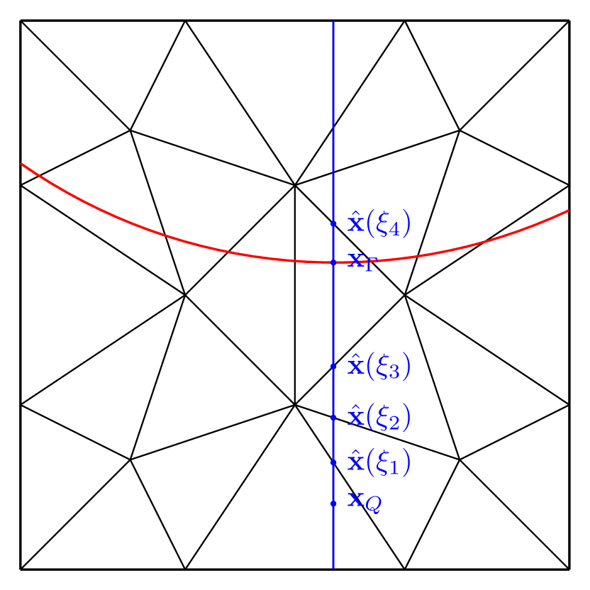
(b) interpolation stencil

Figure 1: Extrapolation into $\mathbf{x}_{Q}$ on a triangular mesh.

6.2 Gradient reconstruction

Having determined the location of $\mathbf{x}_{\Gamma}$, we reconstruct the gradient at that point using finite difference approximations on a uniform stencil aligned with the unit outward normal vector

$$\mathbf{n}_{\Gamma}=-\frac{\mathbf{q}_{h}(\mathbf{x}_{\Gamma})}{|\mathbf{q}_{h}(\mathbf{x}_{\Gamma})|}\approx\mathbf{n}_{+}(\mathbf{x}_{\Gamma}),$$

as shown in Fig. 1(a). The straight line $\hat{\mathbf{x}}(\xi)$ through $\mathbf{x}_{Q}=\hat{\mathbf{x}}(0)$ intersects the inner edge of the diffuse interface region at the point $\mathbf{x}_{P}=\mathbf{x}_{\Gamma}-\epsilon\mathbf{n}_{\Gamma}$. The three-point interpolation stencil

$$\mathcal{S}_{\rm 2D}(\mathbf{x}_{\Gamma})=\{\mathbf{x}_{P}-0.5\epsilon\bm{\tau}_{\Gamma},\mathbf{x}_{P},\mathbf{x}_{P}+0.5\epsilon\bm{\tau}_{\Gamma}\}$$

is constructed using a unit vector $\bm{\tau}_{\Gamma}$ orthogonal to $\mathbf{n}_{\Gamma}$. In the 3D case, the five-point stencil

$$\mathcal{S}_{\rm 3D}(\mathbf{x}_{\Gamma})=\{\mathbf{x}_{P}-0.5\epsilon(\mathbf{n}_{\Gamma}\times\bm{\tau}_{\Gamma}),\mathbf{x}_{P}-0.5\epsilon\bm{\tau}_{\Gamma},\mathbf{x}_{P},\mathbf{x}_{P}+0.5\epsilon\bm{\tau}_{\Gamma},\mathbf{x}_{P}+0.5\epsilon(\mathbf{n}_{\Gamma}\times\bm{\tau}_{\Gamma})\}$$

is used for interpolation purposes. Note that the cross product $\mathbf{n}_{\Gamma}\times\bm{\tau}_{\Gamma}$ is a unit vector orthogonal to $\mathbf{n}_{\Gamma}$ and $\bm{\tau}_{\Gamma}$. Hence, the vectors $\bm{\tau}_{\Gamma}$ and $\mathbf{n}_{\Gamma}\times\bm{\tau}_{\Gamma}$ span the shifted tangential plane at $\mathbf{x}_{P}$.

If a Neumann (rather than Dirichlet) boundary condition is prescribed on $\Gamma(t)$, we use it to define the interface value $\partial_{n}U(\mathbf{x}_{\Gamma})$ directly. Otherwise, we use the Dirichlet value $u_{\Gamma}(\mathbf{x}_{\Gamma})$ and the interpolated value $u_{h}(\mathbf{x}_{\Gamma}-\epsilon\mathbf{n}_{\Gamma})$ to construct the finite difference approximation

$$\partial_{n}U(\mathbf{x}_{\Gamma})=\frac{u_{\Gamma}(\mathbf{x}_{\Gamma})-u_{h}(\mathbf{x}_{\Gamma}-\epsilon\mathbf{n}_{\Gamma})}{\epsilon}$$ (23)

to the normal derivative at $\mathbf{x}_{\Gamma}$. Tangential derivatives are approximated similarly using interpolated values at the points belonging to the interpolation stencil ($\mathcal{S}_{\rm 2D}(\mathbf{x}_{\Gamma})$ in 2D, $\mathcal{S}_{\rm 3D}(\mathbf{x}_{\Gamma})$ in 3D). Since the interface thickness parameter $\epsilon$ is proportional to the mesh size $h$, the reconstructed gradient $\nabla U(\mathbf{x}_{\Gamma})$ represents a consistent approximation to $\nabla u_{h}(\mathbf{x}_{P})$ with $\mathbf{x}_{P}$ approaching $\mathbf{x}_{\Gamma}$ as $h\to 0$.

Remark 4.

If the boundary data function $u_{\Gamma}$ of the continuous problem is defined only on the zero level set $\Gamma(t)$ of the exact level set function $\phi$, it may not be possible to evaluate $u_{\Gamma}$ at $\mathbf{x}_{\Gamma}$. However, in most practical applications $\phi$ is known analytically or a globally defined function $u_{\Gamma}:\Omega\to\mathbb{R}$ has to be evaluated on the “shifted boundary” $\Gamma_{h}(t)$ because the location of $\Gamma(t)$ is unknown.

6.3 Flux extrapolation

To evaluate $G(\phi_{h},u_{h},u_{\Gamma})$, as defined by (22), at the point $\mathbf{x}_{Q}$, we need the values of $\partial_{n}U(\mathbf{x}_{Q})$ and $U(\mathbf{x}_{Q})$. Since we are using a $\mathbb{P}_{1}$ or $\mathbb{Q}_{1}$ finite element approximation, constant extrapolation

$$\partial_{n}U(\mathbf{x}_{Q})=\partial_{n}U(\mathbf{x}_{\Gamma})$$ (24)

is sufficient for the normal derivative. The linear extrapolation formula (cf. [24])

$$U(\mathbf{x}_{Q})=u_{\Gamma}(\mathbf{x}_{\Gamma})+\nabla U(\mathbf{x}_{\Gamma})\cdot(\mathbf{x}_{Q}-\mathbf{x}_{\Gamma})$$ (25)

can be used for extension of interface values. The inviscid component $F$ of the flux $G(\phi_{h},u_{h},u_{\Gamma})$ can also be defined by linearly extrapolating $f_{n}(u_{h}(\mathbf{x}_{\Gamma}),u_{\Gamma}(\mathbf{x}_{\Gamma}))$ as we do in Section 7.3.

Note that extrapolation is performed along the vector $\mathbf{x}_{Q}-\mathbf{x}_{\Gamma}$, which is generally not parallel to the normal $\mathbf{n}_{\Gamma}$ (see Fig. 1(b)). The gradient $\nabla U(\mathbf{x}_{\Gamma})$ to be used in (25) is uniquely defined by the reconstructed normal and tangential derivatives. Its calculation requires a coordinate transformation from the local coordinate system aligned with $\mathbf{n}_{\Gamma}$ to the standard Cartesian reference frame. The corresponding transformation formulas can be found, e.g., in [13]. No transformations need to be performed for the normal derivatives $\partial_{n}U(\mathbf{x}_{\Gamma})$ to be used in (24).

6.4 Ghost penalties

The best way to define a ghost penalty function $u_{\Omega,h}$ for (19) depends on the problem at hand and on the available data. A simple and natural Dirichlet extension is given by

$$u_{\Omega,h}(\mathbf{x}_{Q})=H_{\epsilon}(\phi_{h}(\mathbf{x}_{Q}))u_{h}(\mathbf{x}_{Q})+(1-H_{\epsilon}(\phi_{h}(\mathbf{x}_{Q})))U(\mathbf{x}_{Q}).$$ (26)

Ghost penalties of Neumann type (as mentioned in Remark 1) can be defined, e.g., using

$$\mathbf{g}_{\Omega,h}(\mathbf{x}_{Q})=H_{\epsilon}(\phi_{h}(\mathbf{x}_{Q}))\nabla u_{h}(\mathbf{x}_{Q})+(1-H_{\epsilon}(\phi_{h}(\mathbf{x}_{Q})))\nabla U(\mathbf{x}_{\Gamma}).$$ (27)

This definition corresponds to constant extrapolation of $\nabla U(\mathbf{x}_{\Gamma})$ into $\Omega_{-}(t)$. The dimensions of local penalization parameters $\gamma^{e}=\gamma_{\Omega,h}|_{K^{e}}$ should be chosen in accordance with the type of the extension (Dirichlet: $\gamma_{D}^{e}=\mathcal{O}(h^{-1})$, Neumann: $\gamma_{N}^{e}=\mathcal{O}(h)$). Detailed analysis of ghost penalties is beyond the scope of the present work. However, we envisage that it can be performed following [6, 21].

Implicit treatment of ghost penalties changes the sparsity pattern of the finite element matrix. For that reason, we implement implicit schemes / steady-state solvers using fixed-point iterations

$$L_{h}\big{(}u_{h}^{(k+1)}\big{)}+\int_{\Omega_{h}}\gamma_{\Omega,h}w_{h}u_{h}^{(k+1)}\,{\rm d}{\mathbf{x}} =R_{h}\big{(}u_{h}^{(k)}\big{)}+\int_{\Omega_{h}}\gamma_{\Omega,h}w_{h}u_{\Omega,h}^{(k)}\,{\rm d}{\mathbf{x}},$$

$$L_{h}\big{(}u_{h}^{(k+1)}\big{)}+\int_{\Omega_{h}}\gamma_{\Omega,h}\nabla w_{h}\cdot\nabla u_{h}^{(k+1)}\,{\rm d}{\mathbf{x}} =R_{h}\big{(}u_{h}^{(k)}\big{)}+\int_{\Omega_{h}}\gamma_{\Omega,h}\nabla w_{h}\cdot\mathbf{g}_{\Omega,h}^{(k)}\,{\rm d}{\mathbf{x}}$$

based on a split form $L_{h}\big{(}u_{h}\big{)}=R_{h}\big{(}u_{h}\big{)}$ of the fully discrete problem without penalization (using $\gamma_{\Omega,h}=0$). One iteration may suffice if the problem is time dependent and the time step is small.

Remark 5.

In our numerical studies for the linear advection equation (see Section 7.3), we found it useful to perform mass lumping for $\int_{\Omega_{h}}\gamma_{\Omega,h}w_{h}u_{h}\,{\rm d}{\mathbf{x}}$ but not for $\int_{\Omega_{h}}\gamma_{\Omega,h}w_{h}u_{\Omega,h}\,{\rm d}{\mathbf{x}}$. This treatment of ghost penalty terms makes the method more stable without adversely affecting its accuracy.

6.5 Extension velocities

If the evolution of $\Gamma_{h}(t)$ is driven by interfacial phenomena and only the normal velocity $v_{n}=V|_{\Gamma_{h}}$ is provided by the mathematical model (as in [16, 39]), a velocity field $\mathbf{v}_{h}$ for evolving the level set function $\phi_{h}$ can be constructed using (22) with a suitably defined extension velocity $V$. The value $V(\mathbf{x}_{Q})$ can be determined using constant or linear extrapolation, as in (24) and (25), respectively. For example, suppose that $V(\mathbf{x}_{\Gamma})=\mu\partial_{n}C(\mathbf{x}_{\Gamma})$ is proportional to a (reconstructed) normal derivative $\partial_{n}C(\mathbf{x}_{\Gamma})$ of a concentration field $C$. Then $V(\mathbf{x}_{Q})=V(\mathbf{x}_{\Gamma})$ may be used to define $\mathbf{v}_{h}(\mathbf{x}_{Q})=V(\mathbf{x}_{Q})\mathbf{n}_{Q}$. This way to calculate $\mathbf{v}_{h}(\mathbf{x}_{Q})$ is an efficient alternative to methods that perform a constant extension of $V(\mathbf{x}_{\Gamma})$ in the normal direction by solving a partial differential equation (cf. [2, 8, 38]).

6.6 Damping functions

If the regularized delta function $\delta_{\epsilon}(\phi)$ has a global support, extrapolation needs to be performed at each quadrature point in the fictitious domain. In this case, the cost of numerical integration and matrix assembly can be drastically reduced using damping functions such as

$$D_{\epsilon}(\phi)=H_{\epsilon}(\phi+m\epsilon)-H_{\epsilon}(\phi-m\epsilon),\qquad m\geq 2.$$ (28)

In particular, computations involving $G(\phi_{h},u_{h},u_{\Gamma})$ can be restricted to a narrow band region (cf. [1]) if the compact-support extensions $U_{\epsilon}=D_{\epsilon}(\phi_{h})U$ and $\partial_{n}U_{\epsilon}=D_{\epsilon}(\phi_{h})\partial_{n}U$ are used in (22).

Localized counterparts of the ghost penalty extensions (26) and (27) can be defined as follows:

$$u_{\Omega,h} =H_{\epsilon}(\phi_{h})u_{h}+(1-H_{\epsilon}(\phi_{h}))D_{\epsilon}(\phi_{h})U,$$

$$\mathbf{g}_{\Omega,h} =H_{\epsilon}(\phi_{h})\nabla u_{h}+(1-H_{\epsilon}(\phi_{h}))D_{\epsilon}(\phi_{h})\nabla U.$$

Note that the integrals of $\gamma_{\Omega,h}w_{h}(u_{h}-u_{\Omega,h})$ and $\gamma_{\Omega,h}\nabla w_{h}\cdot\nabla(u_{h}-u_{\Omega,h})$ vanish also in subdomains where $H_{\epsilon}(\phi_{h})=1$. Thus an efficient narrow-band implementation is possible.

For the extension velocity $\mathbf{v}_{h}=(\phi_{h})V\mathbf{q}_{h}$, damping is performed automatically in (20). Indeed, the integral of $w_{h}\mathbf{v}_{h}\cdot\nabla S_{\epsilon}(\phi_{h})$ vanishes in elements in which $S_{\epsilon}(\phi_{h})$ is constant. This compact support property of the advective term speeds up computations. Moreover, there is no need to prescribe unknown values of $\phi$ on inflow boundaries of $\Omega$, while the standard level set method requires so.

7 Test problems and results

In this section, we apply the diffuse level set method to three new test problems. We design them to have closed-form polynomial exact solutions, which are independent of time even if the equation is time-dependent and the interface is moving. Problems of elliptic, parabolic, and hyperbolic type are defined in Sections 7.1–7.3. The numerical results presented in these sections were calculated using the finite element interpolant $\phi_{h}$ of the exact signed distance function $\phi$. In the elliptic case, the interface $\Gamma=\partial\Omega_{+}$ is a fixed embedded boundary. The objective of our study is to quantify the error caused by weak imposition and the proposed numerical treatment of interface conditions. In particular, ghost penalties of Dirichlet and Neumann type, as well as the narrow-band damping functions (28), are tested in this experiment. The parabolic and hyperbolic cases are designed to assess additional errors caused by the motion of the interface $\Gamma(t)$ and by convective fluxes across fixed embedded boundaries, respectively. In Section 7.4, we solve the parabolic problem using (17) and (18) to evolve the level set function $\phi_{h}$ numerically. The normal velocity of the interface is extended into $\Omega$ using extrapolation with damping (as described in Sections 6.5 and 6.6). This experiment illustrates that all components of our diffuse level set algorithm fit together and produce reasonable results in 2D.

Computations for all test cases are performed on uniform quadrilateral meshes using $\epsilon=2h$ and a C++ implementation of the methods under investigation in the open-source finite element library MFEM [3]. The numerical solutions are visualized using the open-source software GlVis [11].

7.1 Elliptic test

The elliptic scenario corresponds to the steady-state limit of (6) with $\mathbf{f}(u)=0$ and $\kappa=1$. We consider the fictitious domain formulation of the boundary value problem

$$\Delta u =0 \quad\text{in }\Omega_{+},$$

$$u =u_{\Gamma} \quad\mbox{on }\Gamma.$$

The domain $\Omega_{+}$ is enclosed by $\Gamma=\{(x,y)\in\mathbb{R}^{2}:(x-0.5)^{2}+(y-0.5)^{2}=0.0625\}=\partial\Omega_{+}$ and embedded into $\Omega=(0,1)^{2}$. The boundary data and analytical solution are given by

$$u_{\Gamma}(x,y,t)=(x-0.5)^{2}-(y-0.5)^{2}=u(x,y,t)\qquad\forall t\geq 0.$$ (29)

In our numerical experiments, we use the constant penalization parameter $\gamma_{D}=h^{-1}$ for the Dirichlet extension $u_{\Omega,h}$ and $\gamma_{N}=h$ for the Neumann extension $\mathbf{g}_{\Omega,h}$.

The $L^{2}$ error of the finite element approximation in the embedded domain $\Omega_{+}$ is approximated by

$$\|u_{h}-u\|_{0,\Omega_{+}}=\sqrt{\int_{\Omega_{h}}H_{\epsilon}(\phi)(u_{h}-u)^{2}\,{\rm d}{\mathbf{x}}}.$$

To keep the integration domain $\Omega_{+,\epsilon}=\{\mathbf{x}\in\Omega\,:\,H_{\epsilon}(\phi(\mathbf{x}))>0\}$ constant on all refinement levels, we use the interface thickness $\epsilon$ of the finest mesh in this formula.

Table 1 summarizes the results of grid convergence studies for the diffuse level set algorithm using Gaussian regularization (15) and four kinds of ghost penalties. The experimental order of convergence (EOC) is approximately 2 for all types of penalization that we compare in this study (Dirichlet and Neumann, without and with multiplication by the damping functions $D_{\epsilon}(\phi)$ defined by (28)). Hence, the restriction of level set extrapolation to the narrow band $\Omega_{\epsilon}:=\mathrm{supp}(D_{\epsilon}(\phi_{h}))$ around the embedded boundary has no adverse effect on the accuracy of the proposed method. The numerical solutions obtained using damped ghost penalties and the mesh size $h=\frac{1}{128}$ are shown in Fig. 2.

$h^{-1}$	full NGP	EOC	damped NGP	EOC	full DGP	EOC	damped DGP	EOC
16	3.61e-03		3.61e-03		2.28e-03		2.28e-03
32	1.05e-03	1.78	1.06e-03	1.77	6.87e-04	1.73	6.87e-04	1.73
64	2.45e-04	2.10	2.61e-04	2.02	1.72e-04	2.00	1.72e-04	2.00
128	5.50e-05	2.15	6.03e-05	2.11	3.97e-05	2.11	3.97e-05	2.11
256	1.25e-05	2.14	1.39e-05	2.12	8.70e-06	2.19	8.70e-06	2.19
512	3.06e-06	2.03	3.42e-06	2.03	1.95e-06	2.15	1.95e-06	2.15
1024	7.37e-07	2.05	8.46e-07	2.01	4.21e-07	2.22	4.21e-07	2.22

Table 1: Elliptic test, $L^{2}$ convergence history for Dirichlet ghost penalties (DGP) and Neumann ghost penalties (NGP). The full version extends boundary data into $\Omega$. The damped version extends into the narrow band $\Omega_{\epsilon}$.

(a) $u_{h}$, damped DGP

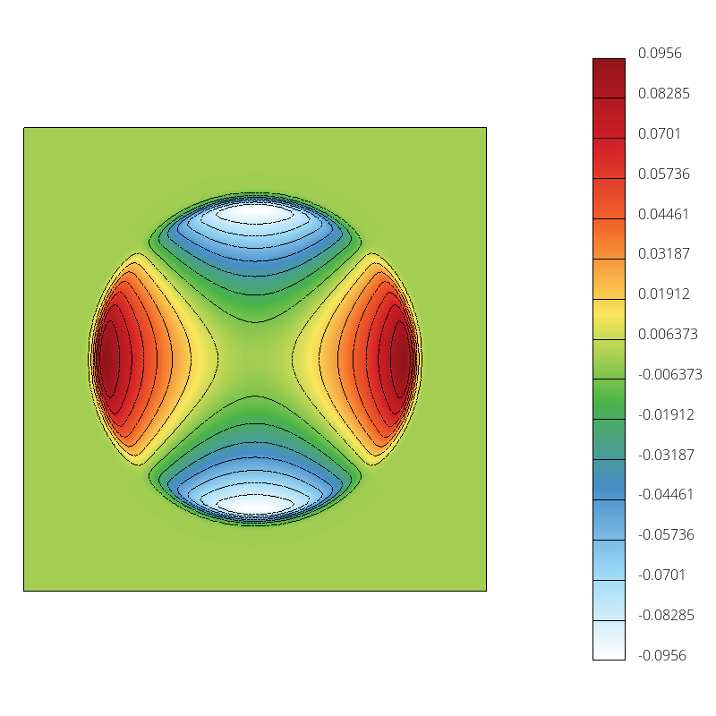
(b) $H_{\epsilon}(\phi)u_{h}$, damped DGP

(c) $u_{h}$, damped NGP

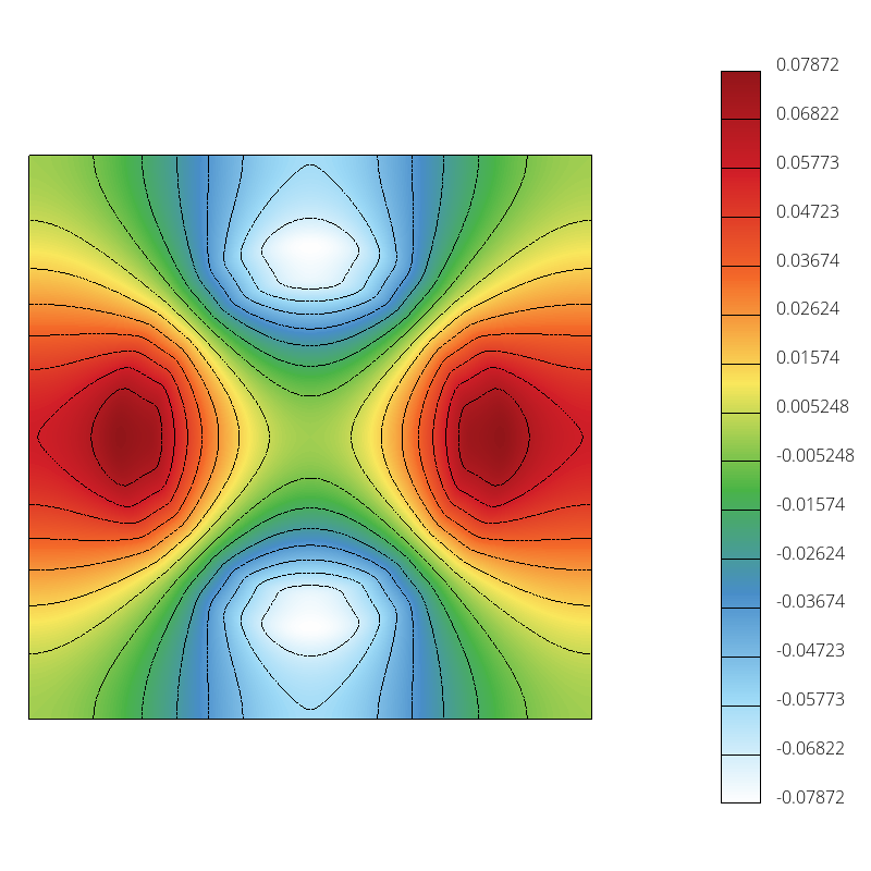
(d) $H_{\epsilon}(\phi)u_{h}$, damped NGP

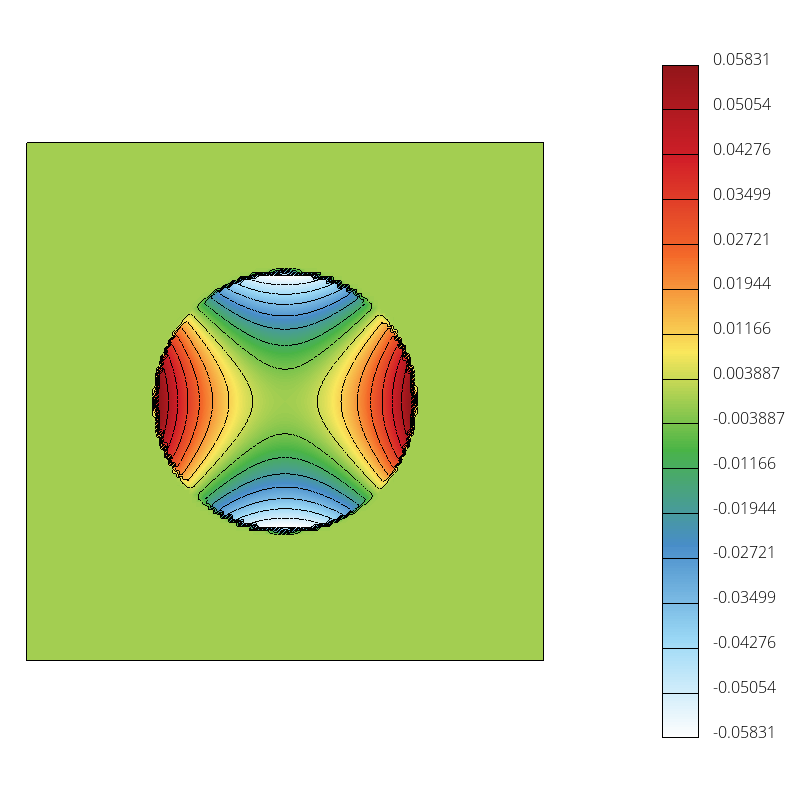
Figure 2: Elliptic test, numerical solutions obtained using $h=\frac{1}{128}$.

7.2 Parabolic test

The parabolic test problem is a time-dependent version of the elliptic case. We solve (6) with $\mathbf{f}(u)=0$ and $\kappa=1$. The initial-boundary value problem is formulated as follows:

$$\frac{\partial u}{\partial t}-\Delta u =0 \quad\text{in }\Omega_{+}(t),$$

$$u =u_{\Gamma} \quad\mbox{on }\Gamma(t),$$

$$u =u_{0} \quad\mbox{in }\Omega_{+}(0).$$

The moving boundary $\Gamma(t)=\{(x,y)\in\mathbb{R}^{2}:(x-0.5)^{2}+(y-0.5)^{2}=(0.25+0.15t)^{2}\}$ is an expanding circle of radius $r(t)=0.25+0.15t$ centered at $(x-0.5,y-0.5)$. The final time $T=1$ is chosen to be short enough for $\Omega_{+}(T)$ to stay embedded in $\Omega=(0,1)^{2}$. As in the elliptic test, the exact solution $u(x,y)$ and the Dirichlet boundary data $u_{\Gamma}(x,y)$ are given by formula (29).

In this example, and in the following ones, we use Dirichlet ghost penalties (DGP). The penalty parameter $\gamma_{D}$ is defined as before. Time discretization is performed using the second-order accurate Crank-Nicolson scheme and the time step $\Delta t=3.2h$ for the parabolic test. The $L^{2}$ errors for numerical solutions at the final time and the corresponding EOCs are presented in Table 2. Second-order convergence behavior is observed again in this experiment. The damped DGP result corresponding to the mesh size $h=\frac{1}{128}$ is shown in Fig. 3.

$h^{-1}$	$(\Delta t)^{-1}$	full DGP	EOC	damped DGP	EOC
16	5	6.30e-03		6.30e-03
32	10	1.16e-03	2.44	1.16e-03	2.44
64	20	2.86e-04	2.02	2.86e-04	2.02
128	40	6.95e-05	2.04	6.95e-05	2.04
256	80	1.67e-05	2.06	1.67e-05	2.06
512	160	4.24e-06	1.98	4.24e-06	1.98
1024	320	1.10e-06	1.95	1.10e-06	1.95

Table 2: Parabolic test, $L^{2}$ convergence history for Dirichlet ghost penalties (DGP). The full version extends boundary data into $\Omega$. The damped version extends into the narrow band $\Omega_{\epsilon}$.

(a) $u_{h}$, damped DGP

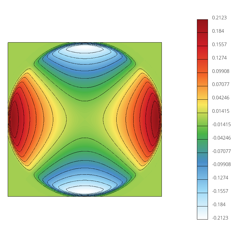
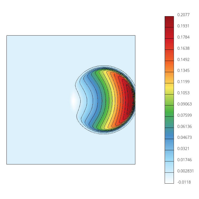
(b) $H_{\epsilon}(\phi)u_{h}$, damped DGP

Figure 3: Parabolic test, numerical solution at $T=1$ obtained using $h=\frac{1}{128}$.

7.3 Hyperbolic test

The third test case is the hyperbolic ($\kappa=0$) limit of (6) with the linear flux $\mathbf{f}(u)=\mathbf{v}u$, where

$$\mathbf{v}(x,y)=(0.5-y,x-0.5)^{T}$$

is a divergence-free rotating velocity field. We solve the solid body rotation problem

$$\frac{\partial u}{\partial t}+\nabla\cdot(\mathbf{v}u) =0 \quad\text{in }\Omega_{+},$$

$$u =u_{\Gamma} \quad\mbox{on }\Gamma_{\rm in},$$

$$u =u_{0} \quad\mbox{in }\Omega_{+},$$

where $\Gamma_{\rm in}$ is the inflow part of $\Gamma(t)=\{(x,y)\in\mathbb{R}^{2}:(x-0.75)^{2}+(y-0.5)^{2}=0.0225\}$ and $\Omega_{+}$ is embedded into $\Omega=(0,1)^{2}$. Computations are stopped at the final time $T=1$. The exact solution

$$u(x,y,t)=(x-0.5)^{2}+(y-0.5)^{2}\qquad\forall t\geq 0$$ (30)

is used to define the boundary data $u_{\Gamma}(x,y,t)$ at the inlet $\Gamma_{\rm in}$ when it comes to constructing $u_{\Omega,h}$.

In this example, the component $F$ of $G(\phi_{h},u_{h},u_{\Gamma})$ is given by the extended upwind approximation

$$F_{Q}(t)=V_{Q}\hat{U}_{Q},$$

where $V_{Q}=\mathbf{v}(x_{\Gamma},y_{\Gamma})\cdot\mathbf{n}_{\Gamma}$ and $\hat{U}(x_{Q},y_{Q},t)$ is the result of linear extrapolation for

$$\hat{u}(x_{\Gamma},y_{\Gamma},t)=\begin{cases}u_{\Gamma}(x_{\Gamma},y_{\Gamma},t)&\mbox{if}\ \mathbf{v}(x_{\Gamma},y_{\Gamma})\cdot\mathbf{n}_{\Gamma}<0,\\ u_{h}(x_{\Gamma},y_{\Gamma},t)&\mbox{if}\ \mathbf{v}(x_{\Gamma},y_{\Gamma})\cdot\mathbf{n}_{\Gamma}\geq 0.\end{cases}$$

The parameter settings for the space discretization are chosen as before. Time integration is performed using Heun’s method, a second-order explicit Runge-Kutta scheme which is known to be strong stability preserving (SSP) under a CFL-type condition. We use the time step $\Delta t=0.5h$ corresponding to the maximum CFL number $\nu=0.25$ in our computations. The results are presented in Table 3 and Fig. 4. In this experiment, the consistent-mass version of the ghost penalty term produced small ripples on fine meshes. The use of mass lumping for $\int_{\Omega_{h}}\gamma_{\Omega,h}w_{h}u_{h}\,{\rm d}{\mathbf{x}}$ (as mentioned in Remark 5) cured this issue. The first-order convergence behavior for the solid body rotation problem is not surprising because we discretize a pure advection equation using the continuous Galerkin method without any stabilization other than mass lumping for the ghost penalty term.

$h^{-1}$	$(\Delta t)^{-1}$	full DGP	EOC	damped DGP	EOC
16	32	4.11e-03		4.11e-03
32	64	2.35e-03	0.81	2.35e-03	0.81
64	128	1.24e-03	0.92	1.24e-03	0.92
128	256	6.45e-04	0.95	6.45e-04	0.95
256	512	3.30e-04	0.97	3.30e-04	0.97
512	1024	1.67e-04	0.98	1.67e-04	0.98
1024	2048	8.40e-05	0.99	8.40e-05	0.99

Table 3: Hyperbolic test, $L^{2}$ convergence history for Dirichlet ghost penalties (DGP). The full version extends boundary data into $\Omega$. The damped version extends into the narrow band $\Omega_{\epsilon}$.

(a) $u_{h}$, damped DGP

(b) $H_{\epsilon}(\phi)u_{h}$, damped DGP

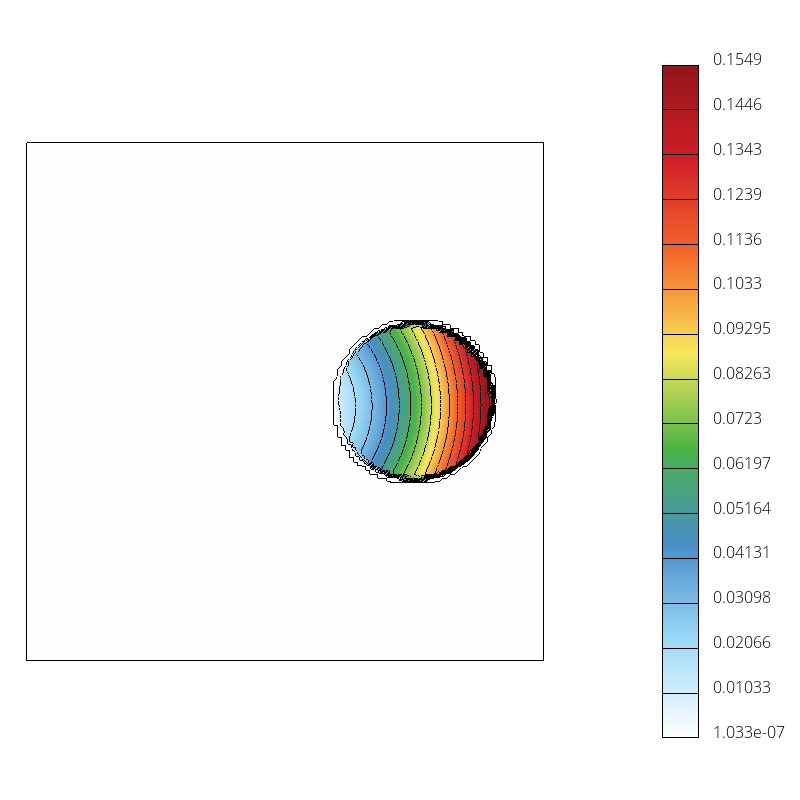
Figure 4: Hyperbolic test, numerical solution at $T=1$ obtained using $h=\frac{1}{128}$.

7.4 Level set advection

In the numerical studies above, we used the finite element interpolant $\phi_{h}$ of the exact signed distance function $\phi$ for extrapolation purposes. In the final test, we use the monolithic conservative level set method [31] to compute a numerical approximation $\phi_{h}$ for the parabolic test problem formulated in Section 7.2. The constant normal velocity $v_{n}=0.15$ of the interface $\Gamma(t)$ is approximated by

$$V(x_{\Gamma},y_{\Gamma},t)=-0.15\partial_{n}\Phi(x_{\Gamma},y_{\Gamma},t),$$

where $\partial_{n}\Phi(x_{\Gamma},y_{\Gamma},t)$ is defined in terms of $\phi_{h}$ similarly to (23). That is, we use

$$\partial_{n}\Phi(x_{\Gamma},y_{\Gamma},t)=\frac{0-\phi_{h}(x_{P},y_{P},t)}{\epsilon}=-\frac{1}{\epsilon}\phi_{h}(x_{P},y_{P},t).$$

Since $\phi(\mathbf{x}_{P},t)=\epsilon$ for the exact SDF evaluated at $\mathbf{x}_{P}=\mathbf{x}_{\Gamma}-\epsilon\mathbf{n}_{\Gamma}$, the so-defined approximate normal derivative should, indeed, satisfy $\partial_{n}\Phi(x_{\Gamma},y_{\Gamma},t)\approx-1$ for $\phi_{h}\approx\phi$. We use constant extrapolation $V(x_{Q},y_{Q},t)=V(x_{\Gamma},y_{\Gamma},t)$ to calculate the extension velocities

$$\mathbf{v}_{h}(x_{Q},y_{Q},t)=-V(x_{Q},y_{Q},t)\mathbf{q}_{h}(x_{Q},y_{Q},t)$$

at quadrature points in the narrow band. Since multiplication by $\nabla S_{\epsilon}(\phi_{h})$ localizes the advective term in (20), no artificial damping functions are used for $\mathbf{v}_{h}$. To verify the accuracy of the algorithm proposed in Section 6.5, we applied it the circular test problem from [38, Section 4.1]. The exact constant extension of $V_{\Gamma}(x,y)=y(1+y)$ defined on $\Gamma=\{(x,y)\in\mathbb{R}^{2}\,:\,\sqrt{x^{2}+y^{2}}=1\}$ is

$$V(x,y)=y\frac{\sqrt{x^{2}+y^{2}}+y}{\sqrt{x^{2}+y^{2}}}.$$

The results obtained with our method and with a continuous Galerkin version of the elliptic extension procedure proposed in [38] are shown in Fig. 5. It can be seen that simple extrapolation performed remarkably well in this preliminary test.

(a) constant extrapolation

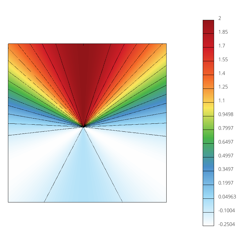
(b) elliptic extension

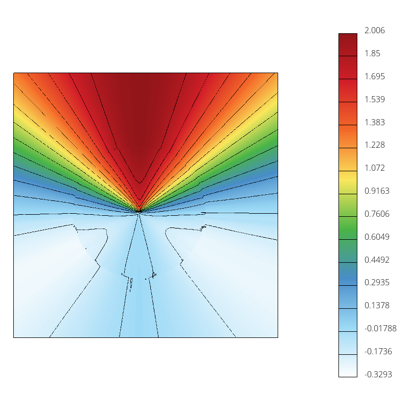
Figure 5: Circular test case [38, Section 4.1], $h=\frac{1}{128}$, extensions constructed using (a) constant extrapolation, as proposed in Section 6.5, and (b) a continuous Galerkin version of the elliptic extension method developed in [38].

In Fig. 6 we present the numerical results for our parabolic test with numerically advected level set function. The snapshots show $u_{h}$ and $\phi_{h}$ at the final time. Both the structure of the exact solution (29) and the circularity of the interface are preserved reasonably well. We also show the signed normal $\mathrm{sign}(\phi_{h})\mathbf{q}_{h}$ of the level set function in Fig. 7. It can be seen that all interface navigation vectors are indeed pointing towards $\Gamma(T)$. A direct comparison with Fig. 3 indicates that disturbances caused by the error of numerical approximation $\phi_{h}\approx\phi$ are of the same order as perturbations caused by other numerical errors. In our experience, the resuls are rather insensitive to the choice of the interface thickness parameter $\epsilon$ (compare Fig. 6 and Fig. 8). We conclude that our approach to construction of extension velocities is a viable option for level set algorithms and other methods.

(a) $H_{\epsilon}(\phi)u_{h}$

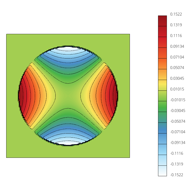
(b) $\phi_{h}$

Figure 6: Parabolic test with numerical level set advection, results obtained with $\epsilon=2h$ at $T=1$.

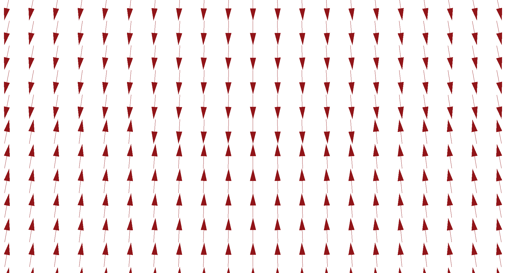
Figure 7: Nodal values of $\mathrm{sign}(\phi_{h})\mathbf{q}_{h}$, a zoom for the bottom side of the interface at $T=1$.

(a) $H_{\epsilon}(\phi)u_{h}$

(b) $\phi_{h}$

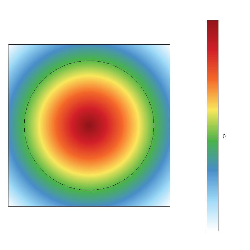
Figure 8: Parabolic test with numerical level set advection, results obtained with $\epsilon=h$ at $T=1$.

8 Conclusions

The unfitted finite element method presented in this paper is based on a new fictitious domain formulation of an initial-boundary value problem for a general time-dependent conservation law. Sharp interface conditions are extended into a diffuse interface. The main focus of our investigations was on proper definition and efficient numerical implementation of narrow-band extension operators. The general framework that we developed for extrapolation of interfacial data features

• a fast closest-point search algorithm that uses a postprocessed gradient of a level set function;

• a new way to define and calculate compact-support extensions of Dirichlet and Neumann type;

• narrow-band integration of terms involving extended fluxes, ghost penalties, and velocity fields.

The same methodology can be used for efficient extrapolation to sharp surrogate boundaries (as in [24]). Theoretical studies of related methods in [6, 19, 21, 22, 24, 41] and other publications provide useful tools for further analysis of the proposed approach. Other promising research avenues include construction of new approximate delta functions with compact supports, extensions to interface problems with jump conditions (as in [22, 40]), special treatment of surfaces with kinks and corners (as in [19]), as well as theory-based design of ghost penalties using Dirichlet and Neumann extensions.

References

- [1] D. Adalsteinsson and J.A. Sethian, A fast level set method for propagating interfaces. J. Comput. Phys. 118 (1995) 269-277.
- [2] D. Adalsteinsson and J.A. Sethian, The fast construction of extension velocities in level set methods. J. Comput. Phys. 148 (1999) 2–22.
- [3] R. Anderson, A. Barker, J. Bramwell, J.-S. Camier, J. Cerveny, V. Dobrev, Y. Dudouit, A. Fisher, Tz. Kolev, W. Pazner, M. Stowell, V. Tomov, J. Dahm, D. Medina, and S. Zampini, MFEM: a modular finite element library. Computers & Mathematics with Applications 81 (2021) 42–74.
- [4] N. M. Atallah, C. Canuto, and G. Scovazzi, Analysis of the shifted boundary method for the Poisson problem in domains with corners. Math. Comp. 90 (2021) 2041–2069.
- [5] J.U. Brackbill, D.B. Kothe, and C. Zemach, A continuum method for modeling surface tension. J. Comput. Phys. 100 (1992) 335-354.
- [6] E. Burman, Ghost penalty. Comptes Rendus Math. 348 (2010) 1217–1220.
- [7] E. Burman, S. Claus, P. Hansbo, M.G. Larson, and André Massing, CutFEM: Discretizing geometry and partial differential equations. Int. J. Numer. Meth. Engrg. 104 (2015) 472–501.
- [8] S. Chen, B. Merriman, S. Osher, and P. Smereka, A simple level set method for solving Stefan problems. J. Comput. Phys. 135 (1997) 8–29.
- [9] J. Chessa, P. Smolinski, and T. Belytschko, The extended finite element method (XFEM) for solidification problems. Int. J. Numer. Meth. Engrg. 53 (2002) 1959–1977.
- [10] B. Engquist, A.K. Tornberg, and R. Tsai, Discretization of Dirac delta functions in level set methods. J. Comput. Phys. 207 (2005) 28–51.
- [11] GlVis: OpenGL Finite Element Visualization Tool. https://glvis.org
- [12] Yu. Gorb, D. Kurzanova, and Yu. Kuznetsov, A robust preconditioner for high-contrast problems. In: B. Acu, D. Danielli, M. Lewicka, A. Pati, R.V. Saraswathy, and M. Teboh-Ewungkem (eds), Advances in Mathematical Sciences 21 (AWM Research Symposium, Houston, TX), Springer, 2020, pp. 289-310.
- [13] H. Hajduk, D. Kuzmin, and V. Aizinger, New directional vector limiters for discontinuous Galerkin methods. J. Comput. Phys. 384 (2019) 308–325.
- [14] P. Hansbo and A. Hansbo, An unfitted finite element method, based on Nitsche’s method, for elliptic interface problems. Comput. Methods Appl. Mech. Engrg. 191 (2002) 5537–5552.
- [15] P. Hansbo, M.G. Larson, and S. Zahedi, A cut finite element method for a Stokes interface problem. Applied Numerical Mathematics 85 (2014) 90–114.
- [16] C.S. Hogea, B.T. Murray and J. A. Sethian, Simulating complex tumor dynamics from avascular to vascular growth using a general level-set method. J. Math. Biol. 53 (2006) 86–134.
- [17] S. Hysing, A new implicit surface tension implementation for interfacial flows. Int. J. Numer. Methods Fluids 51 (2006) 659–672.
- [18] C. Kublik and R. Tsai, Integration over curves and surfaces defined by the closest point mapping. Res. Math. Sci. 3 (2016) 1–17.
- [19] C. Kublik and R. Tsai, An extrapolative approach to integration over hypersurfaces in the level set framework. Math. Comp. 87 (2018) 2365–2392.
- [20] D. Kuzmin, Algebraic flux correction I. Scalar conservation laws. In: D. Kuzmin, R. Löhner and S. Turek (eds.) Flux-Corrected Transport: Principles, Algorithms, and Applications. Springer: Scientific Computation, 2nd edition: 2012, pp. 145–192.
- [21] C. Lehrenfeld and M. Olshanskii, An Eulerian finite element method for PDEs in time-dependent domains. ESAIM: M2AN 53 (2019) 585–614.
- [22] K. Li, N. M. Atallah, A. Main, and G. Scovazzi, The Shifted Interface Method: A flexible approach to embedded interface computations. Int. J. Numer. Meth. Engrg. 121 (2020) 492–518.
- [23] X. Li, J. Lowengrub, A. Rätz, and A. Voigt, Solving PDEs in complex geometries: A diffuse domain approach. Commun. Math. Sci. 7 (2009) 81–107.
- [24] A. Main and G. Scovazzi, The shifted boundary method for embedded domain computations. Part I: Poisson and Stokes problems. J. Comput. Phys. 372 (2018) 972–995.
- [25] A. Main and G. Scovazzi, The shifted boundary method for embedded domain computations. Part II: Linear advection-diffusion and incompressible Navier–Stokes equations. J. Comput. Phys. 372 (2018) 996–1026.
- [26] S. May and M. Berger. An explicit implicit scheme for cut cells in embedded boundary meshes. J. Scientific Computing 71 (2017) 919–943.
- [27] R. Mittal and G. Iaccarino, Immersed boundary methods. Annu. Rev. Fluid Mech. 37 (2005) 239–61.
- [28] B. Müller, F. Kummer, and M. Oberlack, Highly accurate surface and volume integration on implicit domains by means of moment-fitting. Int. J. Numer. Meth. Engrg. 96 (2013) 512–528.
- [29] S. Osher and R. Fedkiw, Level Set Methods and Dynamic Implicit Surfaces. Springer, New York, 2003.
- [30] C.S. Peskin, The immersed boundary method. Acta Numerica 11 (2003) 479–517.
- [31] M. Quezada de Luna, D. Kuzmin, and C.E. Kees, A monolithic conservative level set method with built-in redistancing. J. Comput. Phys. 379 (2019) 262–278.
- [32] M. Quezada de Luna, J.H. Collins, and C.E. Kees, An unstructured finite element model for incompressible two-phase flow based on a monolithic conservative level set method. Int J. Numer. Methods Fluids 92 (2020) 1058–1080.
- [33] J.A. Sethian and P. Smereka, Level set methods for fluid interfaces. Annual Review of Fluid Mechanics 35 (2003) 341–372.
- [34] P. Smereka, The numerical approximation of a delta function with application to level set methods. J. Comput. Phys. 211 (2006) 77–90.
- [35] K.E. Teigen, P. Song, J. Lowengrub, and A. Voigt, A diffuse-interface method for two-phase flows with soluble surfactant. J. Comput. Phys. 230 (2011) 375–393.
- [36] K.E. Teigen, F. Wang, X. Li, J. Lowengrub, and A. Voigt, A diffuse-interface approach for modelling transport, diffusion and adsorption/desorption of material quantities on a deformable interface. Commun. Math. Sci. 7 (2009) 1009–1037.
- [37] J.D. Towers, Two methods for discretizing a delta function supported on a level set. J. Comput. Phys. 220 (2007) 915–931.
- [38] T. Utz and F. Kummer, A high-order discontinuous Galerkin method for extension problems. Int. J. Numer. Methods Fluids 86 (2018) 509–518.
- [39] F.J. Vermolen, E. Javierre, C. Vuik, L. Zhao, and S. van der Zwaag, A three-dimensional model for particle dissolution in binary alloys. Comput. Materials Science 39 (2007) 767–774.
- [40] E. Wadbro, S. Zahedi, G. Kreiss, and M. Berggren, A uniformly well-conditioned, unfitted Nitsche method for interface problems. BIT Numer. Math. 53 (2013) 791–820.
- [41] S. Zahedi and A.K. Tornberg, Delta function approximations in level set methods by distance function extension. J. Comput. Phys. 229 (2010) 2199–2219.