Risk and optimal policies in bandit experiments

Abstract.

We provide a decision theoretic analysis of bandit experiments under local asymptotics. Working within the framework of diffusion processes, we define suitable notions of asymptotic Bayes and minimax risk for these experiments. For normally distributed rewards, the minimal Bayes risk can be characterized as the solution to a second-order partial differential equation (PDE). Using a limit of experiments approach, we show that this PDE characterization also holds asymptotically under both parametric and non-parametric distributions of the rewards. The approach further describes the state variables it is asymptotically sufficient to restrict attention to, and thereby suggests a practical strategy for dimension reduction. The PDEs characterizing minimal Bayes risk can be solved efficiently using sparse matrix routines or Monte-Carlo methods. We derive the optimal Bayes and minimax policies from their numerical solutions. These optimal policies substantially dominate existing methods such as Thompson sampling; the risk of the latter is often twice as high.

1. Introduction

The multi-armed bandit problem describes an agent who seeks to maximize the welfare, i.e., the cumulative returns (aka rewards), generated by sequentially selecting among various actions (aka arms), the effects of which are initially unknown. Compared to classical approaches like RCTs, bandit algorithms enable fast learning and implementation of optimal actions, while minimizing welfare-lowering experimentation. Due to this promise of large welfare gains, they have been extensively studied in recent years and applied in areas such as online advertising (Russo et al., 2017), dynamic pricing (Ferreira et al., 2018), public health (Athey et al., 2021), and, increasingly, in economics (Kasy and Sautmann, 2019; Caria et al., 2020).

The bandit problem can be formulated as a dynamic programming one, but solving this exactly is infeasible. Instead, heuristics based on the exploration-exploitation tradeoff are commonly used, such as Thompson sampling (TS; see Russo et al., 2017 and references therein) and Upper Confidence Bound (UCB; Lai and Robbins, 1985) algorithms. There is by now a large theoretical literature on the regret properties of stochastic bandit algorithms (there is also an important, and parallel, literature on adversarial bandits, that this paper does not contribute to, see, e.g., Hazan et al., 2016). Here, regret is the difference in welfare from pulling the best arm and the agent’s actual welfare. Existing results on lower bounds for regret come in two forms. The first set of results, ‘instance dependent bounds’ (Lai and Robbins, 1985), provide lower bounds on rates of regret for ‘consistent’ algorithms under a given set of reward distributions for each arm. These results are of a large deviations flavor. The second set of results specify the minimax rates of regret, when nature is allowed to adversarially change the reward distributions depending on $n$, the number of periods of experimentation allowed. This rate is of the order $n^{-1/2}$ (Lattimore and Szepesvári, 2020, Ch. 9).

Despite these advances, a number of questions still remain. Many algorithms, including TS and UCB, attain the rate bounds described above, but existing results are silent on selecting between them. Decision theory under ambiguity suggests two common measures, Bayes and minimax risk, for ranking algorithms. The importance of these measures is well recognized in the bandit literature, see Lattimore and Szepesvári (2020, Chs. 13, 35), but their characterization, and the subsequent derivation of optimal algorithms, remain open questions (in fact, a common, but incorrect, view is that these are intractable). We seek to answer these questions.

The first contribution of this paper is to define notions of asymptotic Bayes and minimax risk for bandit experiments under diffusion asymptotics (Wager and Xu, 2021; Fan and Glynn, 2021). These asymptotics consider the regime where the difference in expected rewards between the arms scales at the minimax, $n^{-1/2}$, rate. This defines the hardest instance of the bandit problem: if the reward gap scales at a faster rate, identifying the optimal arm is straightforward, whereas if it scales at a slower rate, there is too little difference between the arms, so the asymptotic risk is trivially 0 in either case. The $n^{-1/2}$ scaling thus provides a good approximation to the finite sample properties of bandit algorithms. The same scaling occurs in the analysis of treatment assignment rules by Hirano and Porter (2009).

Wager and Xu (2021) and Fan and Glynn (2021) study the properties of TS under diffusion asymptotics, but do not address the question of optimal policies under Bayes and minimax risk, as we do here. We define Bayes risk using ‘non-negligible’ priors, i.e., priors applied on the mean rewards after scaling them by the minimax, $n^{-1/2}$, rate (see Section 2.2). This a major departure from the existing literature that, starting from Lai (1987), employs a fixed prior, but which leads to a trivial Bayes risk of $0$ under the $n^{-1/2}$ scaling. This literature instead analyzes Bayes risk using large-deviation methods without scaling the rewards, but as it is based on analysis of tail probabilities and not distributional approximations, the results are not sharp enough to select between various policies, e.g., both TS and UCB attain the large-deviation lower bound. By contrast, we characterize the minimal Bayes risk under the $n^{-1/2}$ scaling as the solution to a $2^{\textrm{nd}}$-order PDE.

We first demonstrate this characterization for Gaussian rewards, using the theory of viscosity solutions to PDEs (Crandall et al., 1992). The PDE machinery is indispensable because existing results (Wager and Xu, 2021; Fan and Glynn, 2021) only apply to continuous policies, whereas the optimal Bayes policy is generically deterministic, and hence discontinuous. Next, using a limit of experiments approach, we show that the same PDE characterization also holds asymptotically under both parametric and non-parametric distributions of the rewards. Thus, any bandit problem can be asymptotically reduced to one with Gaussian rewards. As part of this reduction, we find that it is sufficient to restrict attention to just two state variables per arm, apart from time: these are the number of times the arm has been pulled in the past, and either the score process (for parametric models) or the cumulative rewards from pulling the arm (for nonparametric models). This reduction in dimension is perhaps the main practical insight of this paper since the state space otherwise grows linearly with $n$ (see Section 4.1).

We demonstrate the equivalence of experiments by extending the posterior approximation method of Le Cam and Yang (2000, Section 6.4) to sequential experiments. The proof makes use of novel arguments involving uniform approximation of log-likelihoods and posteriors in sequential settings. It also differs from the standard approach based on asymptotic representations; the latter is difficult to implement under diffusion asymptotics as it requires the construction of couplings between continuous time processes. The techniques introduced here are thus of independent interest for analyzing other types of sequential experiments.

The PDE characterizing minimal Bayes risk is essentially a limit case of the dynamic programming problem (DP) associated with the bandit experiment. While it is infeasible to solve the DP problem directly, we present ways to efficiently solve the PDE using finite-difference and Monte-Carlo methods. This enables us to identify the Bayes optimal policies. Compared to the latter, we find TS to be provably sub-optimal as it over-explores; both theory and empirical illustrations drawn from real-world examples find its Bayes risk to be generally twice as high. Conversely, under independent Gaussian priors, the form of the optimal policy is broadly similar to UCB (for one-armed bandits, this even holds under any prior). In such cases, we show that MOSS, a rate optimal version of UCB, can effectively mimic the optimal policy after optimally tuning it to the given prior. This is borne out by our empirical illustrations and we thus recommend it over TS. Incidentally, such a tuned version of MOSS, while natural, does not appear to have been considered before; in fact, the standard implementation of MOSS performs even worse than TS. It should be noted, however, that the similarity between the optimal policy and UCB/MOSS fails for correlated and non-Gaussian priors.

As an alternative to Bayes risk, we can use minimax risk. This is simply Bayes risk under a least-favorable prior, and we numerically compute both this prior and the minimax optimal policy. Intriguingly, we find that optimally tuned MOSS (as proposed here) is close to minimax optimal for one-armed bandits, even as an optimally tuned TS performs much worse. This highlights the usefulness of our theory since it would not have been possible to know the above without computing the minimax lower bound; existing results give no reason to favor MOSS over TS.

Our framework easily accommodates various generalizations and modifications to the bandit problem such as time discounting and best arm identification (Russo, 2016; Kasy and Sautmann, 2019). The discounted bandit problem has a rich history in economic applications, ranging from market pricing (Rothschild, 1974) to decision making in labor markets (Mortensen, 1986). For discounted problems, the optimal Bayes policy can be characterized using Gittins indices (Gittins, 1979). However, except in simple instances, e.g., discrete state spaces, computing the Gittins index is difficult (see, Lattimore and Szepesvári, 2020, Section 35.5). Also, it does not apply beyond the discounted setting; the optimal Bayes policy in finite horizon settings is not an index policy (Berry and Fristedt, 1985, Chapter 6). Here, we take a different route and characterize the optimal Bayes policy using PDEs.

2. Diffusion asymptotics and statistical risk

In this section, we provide a heuristic derivation of the PDE characterizing minimal Bayes risk in the Multi-Armed Bandit (MAB) problem.

In the MAB problem, there are $K$ arms, and at each period $j$, a decision maker (DM) chooses which arm $k\in\{0,\dots,K-1\}$ to pull. Each pull generates a reward with an unknown mean $\mu_{k}$ that is specific to the arm. Suppose the experiment concludes after $n$ periods, where $n$ is pre-specified. Knowledge of $n$ is reasonable if it is the population size; indeed, the bandit setting blurs any distinction between sample and population. In other cases, it might be more reasonable to assume the DM employs discounting and allows the experiment to continue indefinitely. The decision theoretic analysis employed here requires modeling all aspects of decision making including when to stop or how to discount, but our results are otherwise very broadly applicable. We focus on the known $n$ case to avoid duplication of effort, but see Appendix G.3 for discounted bandits. When $n$ is known, the number of periods that have elapsed is a state variable, and after dividing by $n$ will be termed ‘time’. Thus, time $t$ proceeds from 0 and 1, and is incremented by $1/n$ between successive periods.

Let $A_{j}$ denote the action in period $j$, where $A_{j}=k$ if arm $k$ is pulled. Suppose each time an arm $k$ is pulled, a reward, $Y^{(k)}$, is drawn from the normal distribution $\mathcal{N}(\mu_{k,n},\sigma_{k}^{2})$, where $\mu_{k,n}:=\mu_{k}/\sqrt{n}$. The scaling of the mean reward by $\sqrt{n}$ follows Wager and Xu (2021) and Fan and Glynn (2021) and ensures the signal decays with sample size. The variances, $\sigma_{k}^{2}$, are assumed to be known. In this section and the next, we provide a detailed description of the MAB problem under such normally distributed rewards. The utility of this analysis stems from the fact that more general models - that assume either a parametric or non-parametric distribution of rewards - reduce asymptotically to the normal setting under the limit of experiments approach, see Sections 4 and 5.

In what follows, we represent rewards using the so-called ‘stack-of-rewards representation’ (Lattimore and Szepesvári, 2020, Section 4.6). This entails the following: We exclusively use $j$ to refer to the periods of experimentation, and $i$ to refer to the number of pulls of an arm. $Y_{i}^{(k)}$ denotes the reward at the $i$-th pull of arm $k$, and ${\bf y}_{i}^{(k)}:=\{Y_{i^{\prime}}^{(k)}\}_{i^{\prime}=1}^{i}$ denotes the sequence of rewards after $i$ pulls of that arm. We can imagine that prior to the experiment, nature draws a stack of outcomes, $\{Y_{i}^{(k)}\}_{i=1}^{n}$, corresponding to each arm $k$, and at each period $j$, if $A_{j}=k$, the agent observes the outcome at the top of the stack (this outcome is then removed from the stack). Note that $\{Y_{i}^{(k)}\}_{i=1}^{n}$ are iid conditional on the unknown parameters $\mu_{k}$.

Due to normality of the rewards, the only relevant state variables are the number of times the arm was pulled, $q_{k}(t):=n^{-1}\sum_{j=1}^{\left\lfloor nt\right\rfloor}\mathbb{I}(A_{j}=k)$, the cumulative rewards, $x_{k}(t):=n^{-1/2}\sum_{i=1}^{\left\lfloor nq_{k}(t)\right\rfloor}Y_{i}^{(k)}$, and time $t$ (see Section 4 for a formal argument about the sufficiency of these state variables). The scaling on $x_{k}(t)$ follows Wager and Xu (2021) and is equivalent to rescaling the rewards $Y_{i}^{(k)}$ by the factor $1/\sqrt{n}$. The DM chooses a policy rule $\pi(\cdot)\equiv\{\pi_{k}(\cdot)\}_{k}:\mathcal{S}\rightarrow[0,1]^{K+1}$ that determines the probability of pulling each arm $k$ given the current state $s:=\{\{x_{k},q_{k}\}_{k},t\}$.

Wager and Xu (2021) show that for Lipschitz continuous $\pi$, the evolution of $q_{k}(t)$ and $x_{k}(t)$ in the large $n$ limit is governed by the SDEs

$$dq_{k}(t)=\pi_{k}(s_{t})dt;\quad dx_{k}(t) =\pi_{k}(s_{t})\mu_{k}dt+\sigma_{k}\sqrt{\pi_{k}(s_{t})}dW_{k}(t),$$ (2.1)

where $\{W_{k}(\cdot)\}_{k}$ are independent one-dimensional Brownian motions, and $\pi_{k}(s_{t}):=\pi_{k}(s(t))$. While (2.1) is convenient for heuristics, there is no guarantee that the optimal policy possesses sufficient regularity properties for (2.1) to formally hold. As it turns out, our formal results, in Section 3, do not rely on (2.1).

2.1. Payoff and loss functions

We take the loss function to be cumulative payoffs, where the payoff is $0$ when the experiment concludes at $t=1$. We focus on the regret payoff

$$R(A,\mu)=n^{-1/2}\left\{Y^{(k^{*})}-\sum_{k}Y^{(k)}\mathbb{I}(A=k)\right\},$$ (2.2)

where $k^{*}=\arg\max_{k}\mu_{k}$. It is the difference in rewards between the optimal action, $A^{*}=k^{*}$, and the action $A$. Clearly, regret is just a rescaling of the welfare payoff $W(A,\mu)=-\sum_{k}Y^{(k)}\mathbb{I}(A=k)/\sqrt{n}$. While these payoffs are equivalent under Bayes risk, their behavior under minimax risk is very different. Under the welfare payoff, the minimax policy is trivial and excessively pessimistic: the DM should never pull the arm. By contrast, the minimax risk under regret payoff is non trivial. For this reason, we focus exclusively on regret (as does most of the bandit literature).

Our theory easily extends to other loss criteria, e.g., best arm identification (Kasy and Sautmann, 2019). The latter is discussed in Appendix G.2.

2.2. Bayes risk

Here we introduce asymptotic Bayes risk for bandit experiments.

2.2.1. Priors and posteriors

Suppose the DM places a prior, $m_{0}$, over $\bm{\mu}:=(\mu_{0},\dots,\mu_{K-1})$. When the current state is $s\equiv\{\{x_{k},q_{k}\}_{k},t\}$, the posterior density of $\bm{\mu}$ is

$$p(\bm{\mu}|s)\propto\prod_{k}p_{q_{k}}(x_{k}|\mu_{k};\sigma_{k}^{2})\cdot m_{0}(\bm{\mu});\quad p_{q}(\cdot|\mu;\sigma^{2})\equiv\mathcal{N}(\cdot|q\mu,q\sigma^{2}),$$

where $\mathcal{N}(\cdot|\mu,\sigma^{2})$ is the normal density with mean $\mu$ and variance $\sigma^{2}$. An important property of the posterior is that it depends only on the $\left\lfloor nq_{k}\right\rfloor$ realizations of the rewards, $\{{\bf y}_{nq_{k}}^{(k)}\}_{k}$, from each arm $k$ and is not affected by the past values of the actions (nor by past values of $q_{k}$). Lemma 1 in Appendix E shows that this property holds generally, and is not limited to Gaussian rewards.

Since the prior is applied on the local parameter $\bm{\mu}$, it is asymptotically ‘non-negligible’. In this regard, our approach differs fundamentally from the previous literature (e.g., Lai, 1987) on Bayesian bandits which employs a fixed prior. Our rationale for a ‘non-negligible’ prior is two-fold: First, it provides a better approximation to finite sample properties. Indeed, any prior applied on the actual mean, $\bm{\mu}/\sqrt{n}$, would be flat asymptotically, and its Bayes risk simply $0$ under the $\sqrt{n}$ scaling of mean rewards (in Lai, 1987, the effect of the prior only shows up in large deviation asymptotics). Second, it enables us to characterize minimax risk as Bayes risk under a least favorable prior (see Section 2.4). The least favorable prior is non-negligible.

In practice, we are typically provided with a prior, $\rho_{0}$, on the unscaled mean $\bm{\mu}_{n}=\bm{\mu}/\sqrt{n}$. To apply the methods here, one needs to convert this to a prior, $m_{0}(\cdot)=\rho_{0}(\cdot/\sqrt{n})$, on $\bm{\mu}$. To illustrate, suppose the DM places a Gaussian prior $\mu_{k,n}\sim\mathcal{N}\left(\bar{\mu}_{k,0},\bar{\nu}_{k}^{2}\right)$ that is independent across $k$. We calibrate the scaled prior mean and variance as $\mu_{k,0}=\sqrt{n}\bar{\mu}_{k,0}$ and $\nu_{k}^{2}=n\bar{\nu}_{k}^{2}$, so $\mu_{k}:=\mu_{k,n}/\sqrt{n}\sim\mathcal{N}(\mu_{k,0},\nu_{k}^{2})$. Then, if the current state is $s\equiv\{\{x_{k},q_{k}\}_{k},t\}$, the posterior distribution of $\mu_{k}$ is

$$\mu_{k}|s\sim\mathcal{N}\left(\frac{\sigma_{k}^{-2}x_{k}+\nu_{k}^{-2}\mu_{k,0}}{\sigma_{k}^{-2}q_{k}+\nu_{k}^{-2}},\frac{1}{\sigma_{k}^{-2}q_{k}+\nu_{k}^{-2}}\right).$$ (2.3)

2.2.2. PDE characterization of Bayes and minimal Bayes risk

For a policy $\pi$, we define asymptotic Bayes risk, $V_{\pi}(s)$, as the expected cumulative regret in the diffusion regime, where the expectation is taken conditional on all information until state $s$. The ex-ante Bayes risk of a policy $\pi$ is then $V_{\pi}(0)\equiv V_{\pi}(s_{0})$ where $s_{0}:=\{\{x_{k}=0,q_{k}=0\}_{k},t=0\}$ is the initial state. This is the expected cumulative regret at the outset of the experiment. It can thus be used for ranking candidate policies. We now informally derive a PDE characterization of $V_{\pi}(s)$.

By (2.1), the change to $q_{k}$ and $x_{k}$ in a short time period $\Delta t$ following state $s$ is approximately (henceforth we use $\pi_{k}$ as a shorthand for $\pi_{k}(s)$)

$$\Delta q_{k} \approx\pi_{k}\Delta t;\quad\Delta x_{k}\approx\pi_{k}\mu_{k}\Delta t+\sigma_{k}\sqrt{\pi_{k}}\Delta W(t).$$

For a given $\bm{\mu}$, the regret, $\Delta V_{\pi,\bm{\mu}},$ accrued within this time period is the difference between the rewards, $\left(\mu_{k^{*}}\Delta t+\sigma_{k^{*}}\Delta W_{k^{*}}(t)\right)$ and $\sum_{k}\Delta x_{k}$, generated, respectively, under the infeasible optimal policy $\mathbb{I}(A_{j}=k^{*})$ and the given policy $\pi$:

$$\Delta V_{\pi,\bm{\mu}}\approx\left(\mu_{k^{*}}-\sum_{k}\mu_{k}\pi_{k}\right)\Delta t+\left\{\sigma_{k^{*}}\Delta W_{k^{*}}(t)-\sum_{k}\sigma_{k}\sqrt{\pi_{k}}\Delta W_{k}(t)\right\}.$$ (2.4)

The recursive nature of the problem implies

$$V_{\pi}(s)=\mathbb{E}\left[\left.\Delta V_{\pi,\bm{\mu}}+V_{\pi}\left(\{x_{k}+\Delta x_{k},q_{k}+\Delta q_{k}\}_{k},t+\Delta t\right)\right|s\right],$$ (2.5)

with the terminal condition $V_{\pi}(s)=0$ if $t=1$.

Now, for the right-hand side of (2.5), the approximation (2.4) implies

$$\mathbb{E}\left[\left.\Delta V_{\pi,\bm{\mu}}\right|s\right] \approx\left(\mathbb{E}_{\bm{\mu}|s}\left[\mu_{k^{*}}-\sum_{k}\mu_{k}\pi_{k}\right]\right)\cdot\Delta t=\left(\mu^{\max}(s)-\sum_{k}\mu_{k}(s)\pi_{k}\right)\cdot\Delta t,$$

where $\mu^{\max}(s):=\mathbb{E}_{\bm{\mu}|s}[\max_{k}\mu_{k}]$ and $\mu_{k}(s):=\mathbb{E}_{\mu_{k}|s}[\mu_{k}]$. Next, by Ito’s lemma,

$$\mathbb{E}\left[\left.V_{\pi}\left(\{x_{k}+\Delta x_{k},q_{k}+\Delta q_{k}\}_{k},t+\Delta t\right)-V_{\pi}(s)\right|s\right]$$

$$\approx\partial_{t}V_{\pi}+\sum_{k}\left\{\pi_{k}\partial_{q_{k}}V_{\pi}+\pi_{k}\mu_{k}(s)\partial_{x_{k}}V_{\pi}+\frac{1}{2}\pi_{k}\sigma_{k}^{2}\partial_{x_{k}}^{2}V_{\pi}\right\}\Delta t.$$

Thus, subtracting $V_{\pi}(s)$ from both sides of (2.5) and dividing by $\Delta t$, we obtain the following characterization of $V_{\pi}$:

$$\partial_{t}V_{\pi}+\mu^{\max}(s)+\sum_{k}\pi_{k}(s)\left\{-\mu_{k}(s)+L_{k}[V_{\pi}](s)\right\} =0\ \textrm{if }t<1,$$ (2.6)

$$V_{\pi}(s) =0\ \textrm{if }t=1.$$

Here, $L_{k}[\cdot]$ denotes the infinitesimal generator

$$L_{k}[f]:=\partial_{q_{k}}f+\mu_{k}(s)\partial_{x_{k}}f+\frac{1}{2}\sigma_{k}^{2}\partial_{x_{k}}^{2}f.$$

Since $\{\sigma_{k}^{2}\}_{k}$ is known, PDE (2.6) can be solved for any candidate $\pi$.

We can also characterize the minimal Bayes risk $V_{\pi}^{*}(s):=\inf_{\pi(\cdot)\in\Pi}V_{\pi}(s)$, where $\Pi$ denotes the class of all measurable policy rules. By the dynamic programming principle, the minimal Bayes risk satisfies

$$V^{*}(s)=\inf_{\pi\in[0,1]}\mathbb{E}\left[\left.\Delta V_{\mu,\pi}+V^{*}\left(\{x_{k}+\Delta x_{k},q_{k}+\Delta q_{k}\}_{k},t+\Delta t\right)\right|s\right],$$

for any small time increment $\Delta t$, together with the boundary condition $V^{*}(s)=0$ if $t=1$. Then, by similar heuristic arguments as those leading to (2.6), we obtain

$$\partial_{t}V^{*}+\mu^{\max}(s)+\min_{k}\left\{-\mu_{k}(s)+L_{k}[V^{*}](s)\right\} =0\ \textrm{if }t<1,$$ (2.7)

$$V^{*}(s) =0\ \textrm{if }t=1.$$

As with PDE (2.6), PDE (2.8) can be solved using knowledge only of $\{\sigma_{k}^{2}\}_{k}$. We can thus characterize the minimal ex-ante Bayes risk as $V^{*}(0):=V^{*}(s_{0})$.

PDE (2.8) encapsulates the exploration-exploitation tradeoff. The regret payoff can be minimized to 0 when the posterior distribution collapses to a point, in which case one chooses the optimal arm with certainty. This is reflected in the fact that the regret payoffs are one of $\{\mu^{\max}(s)-\mu_{k}(s)\}_{k}$, all of which are always greater than $0$, but $\min_{k}\{\mu^{\max}(s)-\mu_{k}(s)\}\to 0$ as $q_{k}$ increases. The DM thus faces a tradeoff between exploration, i.e, pulling the arm enough times to increase the value of $q_{k}$ and thereby reduce $\{\mu^{\max}(s)-\mu_{k}(s)\}_{k}$ in the future, and exploitation, i.e., choosing the best action, $\operatorname*{arg\,max}_{k}\mu_{k}(s)$, at the present.

If a classical, i.e., twice continuously differentiable, solution, $V^{*}(\cdot)$, to PDE (2.8) exists, the optimal Bayes policy is $\pi^{*}(s)=\operatorname*{arg\,min}_{k}\{L_{k}[V^{*}](s)-\mu_{k}(s)\}$. While a classical solution to (2.8) is generally impossible, one can construct measurable policies whose Bayes risk is arbitrarily close to $V^{*}(\cdot)$, and this is all that is needed in practice. One such construction is provided in Section 3.3.

2.2.3. A special case: one-armed bandits

The one-armed bandit is a special case of the MAB problem with two arms and with arm $0$ corresponding to a known outside option. We normalize the reward from the outside option to $0$, i.e., $\mu_{0}=0$ and $\sigma_{0}=0$. The set of sufficient statistics can then be reduced to $s\equiv\{x(t):=x_{1}(t),q(t):=q_{1}(t),t\}$. Let $\mu:=\mu_{1}$ and $\sigma^{2}:=\sigma_{1}$ denote the mean and variance of arm 1. For Bayesian analysis, we place a prior $m_{0}$ on the unknown $\mu$. The PDE characterization of minimal Bayes risk, $V^{*}$, then simplifies to

$$\partial_{t}V^{*}+\mu^{+}(s)+\min\left\{-\mu(s)+L[V^{*}](s),0\right\} =0\ \textrm{if }t<1,$$ (2.8)

with the terminal condition $V^{*}(s)=0$ if $t=1$, where $\mu^{+}(s):=\mathbb{E}_{\mu|s}[\max\{\mu,0\}]$, $\mu(s):=\mathbb{E}_{\mu|s}[\mu]$ and $L[f]:=\partial_{q}f+\mu(s)\partial_{x}f+\frac{1}{2}\sigma^{2}\partial_{x}^{2}f$. We make frequent reference to one-armed bandits in what follows as the reduced state space enables us to describe our theoretical results with minimal notational overhead while still preserving the essential conceptual features of the MAB problem.

For one-armed bandits, it is easy to see that the optimal policy has to be a retirement policy, i.e., if the DM did not pull the arm at some time $t$, she will not do so at any other time in the future. Also, it has to be non-decreasing in $x$. These properties imply $\pi^{*}(s)$ is of the form $\mathbb{I}\left\{x>f(q,t)\right\}$, with $f(\cdot)$ non-decreasing in $t$.

2.3. Comparison with existing methods

Perhaps the two most commonly used algorithms for MAB problems are TS and UCB. The TS rule is $\pi_{k}^{\textrm{ts}}(s)=\mathbb{P}\left(\mu_{k}\geq\max_{k^{\prime}}\mu_{k^{\prime}}|s\right)$ and its asymptotic Bayes risk can be obtained by solving (2.6). Figure 2.1 compares this with the corresponding minimal Bayes risk for one-armed bandits under Gaussian priors, obtained by solving PDE (2.8). For the numerical comparison, we set the prior mean to $0$ and vary the prior and error variances, $\nu^{2}$ and $\sigma^{2}$. To interpret the ranges of $\nu^{2},\sigma^{2}$, note that the unscaled prior variance is $\nu^{2}/n$ (which is why $\nu>\sigma$) and all the policies considered here are invariant to $\nu/\sigma$; for reference, our empirical application in Section 6.3 uses $\nu/\sigma\approx 15$. TS is inferior to the optimal Bayes policy across all parameter values and substantially so - its Bayes risk is generally twice as high.

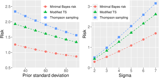
Note: The default parameter values are $\mu_{0}=0$, $\nu=50$ and $\sigma=5$. Modified TS refers to the Thompson sampling rule modified so that $\pi=1$ whenever $x\geq 0$.

Figure 2.1. Asymptotic risk of various policies under one-armed bandits

Figure 2.2 plots the associated optimal policy rule, under the parameter values $(\nu=50,\sigma=5)$, as a function of $x,q$ at a few different snapshots in time. As conjectured earlier, it is of the form $\pi^{*}(s)=\mathbb{I}\{x\geq f(q,t)\}$ with $f(\cdot)$ increasing in $t$. The policy recommends pulling the arm for some $x<0$, even though this indicates negative expected rewards, $\mu(s)$. This is an example of exploration. The extent of exploration, i.e., the values of $x$ for which $\pi^{*}(s)=1$, declines over time. The figure also plots a heat-map of, $\pi^{\textrm{ts}}(\cdot)$, the TS rule. The reason why $\pi^{\textrm{ts}}(\cdot)$ is inferior is simple: it over-explores. TS continuously attempts to trade-off exploration and exploitation against each other, but these motives are not always at odds. Indeed, when $x\geq 0$, pulling the arm is optimal for both exploitation (since the posterior mean is positive) and exploration. A simple modification to the TS rule, that sets $\pi=1$ whenever $x\geq 0$ but is otherwise equivalent to TS, thus delivers 15-20% lower Bayes risk under our one-armed bandit setups, as Figure 2.1 illustrates. More generally, for MABs, we can improve the Bayes risk of TS by modifying it as follows: whenever there exist arms $k,k^{\prime}$ such that $\mu_{k}(s)<\mu_{k^{\prime}}(s)$ and $\textrm{Var}[\mu_{k}|s]\leq\textrm{Var}[\mu_{k^{\prime}}|s]$, we should transfer all the probability that TS assigns to $k$ to $k^{\prime}$ (this can be repeated for all $k,k^{\prime}$).

      

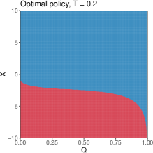
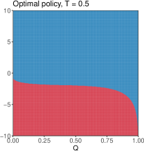
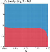
Note: The parameter values are $\mu_{0}=0$, $\nu=50$ and $\sigma=5$. Red corresponds to not pulling the arm while blue corresponds to pulling the arm.

Figure 2.2. Policy maps for a one-armed bandit

On the other hand, the optimal policy shares some similarities with UCB algorithms. Note that $\hat{\mu}:=x/q\sqrt{n}$ is the MLE estimator of the sample mean $\mu/\sqrt{n}$. Then, defining $F(q,t)=-f(q,t)/q$, we find that the optimal policy for one-armed bandits has the form $\pi^{*}=\mathbb{I}\left\{\hat{\mu}+F(q,t)/\sqrt{n}\geq 0\right\}$. We can thus interpret $F(q,t)/\sqrt{n}$ as the optimal confidence width in that setting. More generally, for the MAB problem, if the prior is normal and independent across arms, $\mu_{k}(s)$ is a function only of $x_{k},q_{k}$ and monotonically increasing in $\hat{\mu}_{k}=x_{k}/q_{k}\sqrt{n}$. We can then rewrite the optimal policy in the UCB form $\pi^{*}=\operatorname*{arg\,max}_{k}\{\hat{\mu}_{k}+F_{k}(s)/\sqrt{n}\}$, even if, unlike a typical UCB, $F_{k}(\cdot)$ depends on all of $s$ instead of just $x_{k},q_{k}$. For correlated priors, however, the optimism principle fails and the optimal policy may be very different from UCB; indeed, it can even be optimal to pull an arm with a lower UCB than the others if it is highly informative about the common parameter.

The vanilla UCB policy uses the confidence width $\sqrt{2\sigma^{2}\ln(1/\delta)/nq_{k}}$ for each arm $k$, where $\delta$ is a tuning parameter. But this is far from optimal. For two-armed bandits, Kalvit and Zeevi (2021) show that it converges to a fixed (i.e., non-adaptive) allocation rule under diffusion asymptotics, for any given $\delta,\mu_{1},\mu_{0}$. Consequently, there is no learning (asymptotically) for this class of UCBs, and their Bayes risk can be made arbitrarily large by increasing the prior variance; in fact, their minimax rate of regret is $O(\sqrt{\log n/n})$.

The minimax optimal rate, $O(n^{-1/2})$, can be regained with a more refined confidence width, as evidenced by the MOSS algorithm which uses $\sqrt{2\sigma^{2}g(q_{k})/nq_{k}}$, where $g(q)\approx\ln q^{-1}$. In fact, by Lai (1987), this is an approximation, as $q\to 0$, of the optimal width, $F(q,t)/\sqrt{n}$, in the one-armed setting with a flat prior (i.e., when $\nu^{2}\to\infty$). More generally, with multiple arms and independent Gaussian priors, Section 6 shows that while the standard implementation of MOSS performs a lot worse than the optimal policy, an optimally tuned MOSS, that uses the confidence width $\sqrt{\gamma g(q_{k})/nq_{k}}$, comes close to attaining the risk lower bound. Our proposal for the optimal $\gamma$ here is to choose the value that minimizes the local asymptotic Bayes risk of MOSS under the given prior. It appears that with this choice of $\gamma$, $\sqrt{\gamma\ln q_{k}^{-1}/q_{k}}$ can well-approximate $F_{k}(s)$ under independent Gaussian priors. The optimal $\gamma$ is, however, very sensitive to the prior.

2.4. Minimax risk

Following Wald (1945), we define minimax risk as the value of a two player zero-sum game played between nature and the DM. Nature’s action consists of choosing a prior, $m_{0}\in\mathcal{P}$, over $\bm{\mu}$, while the DM chooses the policy rule $\pi$. The minimax risk $\bar{V}^{*}$ is defined as

$$\bar{V}^{*}=\sup_{m_{0}\in\mathcal{P}}V^{*}(0;m_{0})=\sup_{m_{0}\in\mathcal{P}}\inf_{\pi\in\Pi}V_{\pi}(0;m_{0}),$$ (2.9)

where $V_{\pi}(0;m_{0})$ and $V^{*}(0;m_{0})$ denote the ex-ante Bayes risk under a policy $\pi$, and the minimal Bayes risk, when the prior is $m_{0}$. The equilibrium action of nature is termed the least-favorable prior, and that of the DM, the minimax policy. Under a minimax theorem, which holds if there is a Nash equilibrium to the game (with proper priors), the $\sup$ and $\inf$ operations in (2.9) can be interchanged, so that

$$\sup_{m_{0}\in\mathcal{P}}\inf_{\pi\in\Pi}V_{\pi}(0;m_{0})=\inf_{\pi\in\Pi}\sup_{m_{0}\in\mathcal{P}}V_{\pi}(0;m_{0})=\inf_{\pi\in\Pi}\sup_{\bm{\mu}}V_{\pi}(0;\bm{\mu}).$$ (2.10)

Here, $V_{\pi}(0;\bm{\mu})$ denotes the frequentist risk of a policy $\pi$ when the local parameter is $\bm{\mu}$. The last term, $\inf_{\pi\in\Pi}\sup_{\bm{\mu}}V_{\pi}(0;\bm{\mu})$, is perhaps the more common definition of minimax risk. Thus, by (2.10), the problem of computing minimax risk reduces to that of computing Bayes risk under the least favorable prior.

For one-armed bandits, we conjecture, and verify numerically by solving the two player game, that the least favorable prior, $m_{0}^{*}$, involves only two support points at $\{\text{$\underline{\mu}$},\bar{\mu}\}$, with $\text{$\underline{\mu}$}<0$ and $\bar{\mu}>0$. This is because both low and high values of $|\mu|$ are associated with low risk, the former by definition, and the latter because the DM quickly learns to always pull or never pull the arm. Indeed, for $\sigma=1$, it turns out $m_{0}^{*}$ has a two point support at $\underline{\mu}$ $\approx$ -2.5 and $\bar{\mu}\approx 1.7$ with $m_{0}^{*}(\bar{\mu})\approx 0.415$. It also suffices to solve the game under $\sigma=1$ as we can always rescale the rewards to have unit variance (the risk comparisons are invariant to scale transformations).

Based on the above analysis, we find that the sharp lower bound on the (unscaled) minimax risk of any one-armed bandit algorithm is given by $0.373\sigma\sqrt{n}$. This substantially improves on existing theoretical results which only demonstrate a $\sigma\sqrt{n}$ rate.

Computing the least favorable prior when there are more than two arms is a lot more demanding. We conjecture, however, that it has a discrete support.

3. Formal properties under gaussian rewards

For simplicity, the results in this section are stated for the one-armed bandit problem. However, all our results extend to the general MAB problem with straightforward adjustments to the proofs, see Appendix G.1.

3.1. Existence and uniqueness of PDE solutions

Equation (2.8) describes a nonlinear $2^{\textrm{nd}}$-order PDE. It is well known that such PDEs do not admit classical, i.e., twice continuously differentiable, solutions. Instead, the relevant weak solution concept is that of a viscosity solution (Crandall et al. 1992).

Theorem 1.

(Barles and Jakobsen, 2007, Theorem A.1) Suppose $\mu^{+}(\cdot),\mu(\cdot)$ are $\gamma$-Hölder continuous for some $\gamma>0$. Then there exists a unique, $\gamma$-Hölder continuous viscosity solution to PDE (2.8).

3.2. Convergence to the PDE solution

In Section 2, we provided a heuristic derivation of PDE (2.8). For a formal result, one would need to prove that a discrete analogue, $V_{n}^{*}(\cdot)$, of $V^{*}(\cdot)$, defined for a fixed $n$, converges to $V^{*}(\cdot)$ as $n\to\infty$. Define $\mathbb{I}_{n}=\mathbb{I}\{t\leq 1-1/n\}$ and $Y_{i}$ as the $i$-th realization of the rewards (corresponding to the $i$-th pull of the arm). Let $V_{n}^{*}(\cdot)$ denote the solution to the recursive equation

$$V_{n}^{*}\left(x,q,t\right) =\min_{\pi\in[0,1]}\mathbb{E}\left[\left.\frac{\mu^{+}(s)-\pi\mu(s)}{n}+\mathbb{I}_{n}\cdot V_{n}^{*}\left(x+\frac{A_{\pi}Y_{nq+1}}{\sqrt{n}},q+\frac{A_{\pi}}{n},t+\frac{1}{n}\right)\right|s\right];$$

$$\quad\textrm{if }t<1,$$

$$V_{n}^{*}\left(x,q,1\right) =0.$$ (3.1)

In (3.1), $A_{\pi}\sim\textrm{Bernoulli}(\pi)$, and the expectation is a joint one over $Y_{nq+1},A_{\pi}$ given $s$. Existence of a unique $V_{n}^{*}(\cdot)$ follows by backward induction. Clearly, $V_{n}^{*}(\cdot)$ is the minimal Bayes risk in the fixed $n$ setting under Gaussian rewards. We can thus interpret (3.1) as a discrete approximation to PDE (2.8). As such, it falls under the abstract framework of Barles and Souganidis (1991) for showing convergence to viscosity solutions. An application of their techniques proves the following result (the proof is in Appendix A.1): Denote $\varpi(s):=\min\left\{\mu^{+}(s)-\mu(s),\mu^{+}(s)\right\}$.

Theorem 2.

Suppose $\mu^{+}(\cdot),\mu(\cdot)$ are $\gamma$-Hölder continuous, $\sup_{s}\varpi(s)<\infty$ and the prior $m_{0}$ is such that $\mathbb{E}[|\mu|^{3}|s]<\infty$ at each $s$. Then, as $n\to\infty$, $V_{n}^{*}(\cdot)$ converges locally uniformly to $V^{*}(\cdot)$, the unique viscosity solution of PDE (2.8).

The assumptions are satisfied for Gaussian priors. Note also that the theorem is proved without appealing to (2.1). In Appendix B we derive a coarse upper bound on the rate of convergence of $V_{n}^{*}(\cdot)$ to $V^{*}(\cdot)$ and provide simulation evidence suggesting that the quality of the approximation is quite good in practice.

3.3. Piece-wise constant policies and batched bandits

While we are not able to characterize the optimal Bayes policy in closed form, it is possible to construct (Lebesgue) measurable policies whose Bayes risk is arbitrarily close to $V^{*}(\cdot)$. One way to do so is using piece-wise constant policies. In fact, a bandit experiment with such a policy is equivalent to a batched bandit experiment, where the data is forced to be considered in batches. The results in this section thus give an upper bound on the welfare loss due to batching.

Let $\Delta t$ denote a small time increment, and $\mathcal{T}_{\Delta t}:=\{t_{1},\dots,t_{L}\}$ a set of grid points for time, where $t_{1}=0$, $t_{L}=1$ and $t_{l}-t_{l-1}=\Delta t$ for all $l$. The optimal piece-wise constant policy, $\pi_{\Delta t}^{*}:\mathcal{X}\times\mathcal{Q}\times\mathcal{T}_{\Delta t}\mapsto\{0,1\}$, is allowed to change only at the time points on the grid $\mathcal{T}_{\Delta t}$. In particular, suppose that $x=x_{l}$ and $q=q_{l}$ at the grid point $t=t_{l}$. Then one computes $\pi_{\Delta t}^{*}(x_{l},q_{l},t_{l})\in\{0,1\}$ and holds this policy value fixed until the next time point $t_{l+1}$. Define $V_{\Delta t,l}^{*}(x,q)$ as the Bayes risk, in the diffusion regime, at state $(x,q,t_{L-l})$ under $\pi_{\Delta t}^{*}(\cdot).$ We then have the following recursion for $V_{\Delta t,l}^{*}(x,q)$:

$$V_{\Delta t,l+1}^{*}(x,q) =\min\left\{S_{\Delta t}\left[V_{\Delta t,l}^{*}\right](x,q),V_{\Delta t,l}^{*}(x,q)+\Delta t\cdot\mu^{+}(x,q)\right\},\ l=0,\dots,L-1,$$

$$V_{\Delta t,0}^{*}(x,q) =0,$$ (3.2)

where the operator $S_{\Delta t}[\phi](x,q)$ denotes the solution at $(x,q,\Delta t)$ of the linear second order PDE

$$-\partial_{t}f(s)+\mu^{+}(s)-\mu(s)+L[f](s) =0,\ \textrm{if }t>0;\quad f=\phi,\ \textrm{if }t=0.$$ (3.3)

The following theorem assures that $V_{\Delta t,l}^{*}(\cdot)$ can be made arbitrarily close to $V^{*}(\cdot,\cdot,t_{L-l})$ by letting $\Delta t\to 0$.

Theorem 3.

(Jakobsen et al., 2019, Theorem 2.1) Suppose $\mu^{+}(\cdot),\mu(\cdot)$ are Lipschitz continuous. Then there exists $C<\infty$ that depends only on the Lipschitz constants of $\mu^{+}(\cdot),\mu(\cdot)$ such that $0\leq\max_{l}\left\{V_{\Delta t,l}^{*}(\cdot)-V^{*}(\cdot,t_{L-l})\right\}\leq C(\Delta t)^{1/4}$ uniformly over $\mathcal{X}\times\mathcal{Q}$.

Note that $\pi_{\Delta t}^{*}(\cdot)$ is not required to converge to some measurable $\pi^{*}(\cdot)$ as $\Delta t\to 0$. Still, we can employ $\pi_{\Delta t}^{*}(\cdot)$ in the fixed $n$ setting: to apply, one simply sets $t=\left\lfloor i/n\right\rfloor$, where $i$ is the current period. The following theorem asserts that employing $\pi_{\Delta t}^{*}(\cdot)$ in this manner results in a Bayes risk that is arbitrarily close to $V^{*}(0)$.

Theorem 4.

Suppose $\mu^{+}(\cdot),\mu(\cdot)$ are Lipschitz continuous and $\sup_{s}\mu^{+}(s)<\infty$. Then, for any fixed $\Delta t$, $\lim_{n\to\infty}\left|V_{\pi_{\Delta t}^{*},n}(0)-V^{*}(0)\right|\leq C(\Delta t)^{1/4}$ .

4. General parametric models

We now relax the Gaussian assumption, and suppose that rewards are distributed according to some parametric model $P_{\theta}$, with $\theta$ unknown. In general, a dynamic-programming solution to the optimal Bayes policy in this setting involves a state space of dimension $O(n)$. However, we show that it is possible to reduce this asymptotically to just two state variables per arm (apart from time): the number of times the arm has been pulled, and the score process, i.e., the cumulative sum of scores scaled by $n^{-1/2}$, where the scores correspond to the distribution of rewards for that arm. All our results previously derived for Gaussian models then continue to apply after simply reinterpreting $x_{k}(t)$ as the score process. Underlying these claims is a posterior approximation result that states that the posterior density of the parametric model can be uniformly approximated, at every point in time, by that from a Gaussian model.

For the rest of this section, we focus on the one-armed bandit for simplicity. We start by assuming $\theta$ to be scalar to simplify notation, but the vector case (discussed in Section 4.3) does not otherwise present any new conceptual difficulties. The mean rewards are denoted by $\mu(\theta)\equiv\mathbb{E}_{P_{\theta}}[X]$. As in Hirano and Porter (2009), we focus on local perturbations of the form $\{\theta_{n,h}\equiv\theta_{0}+h/\sqrt{n}:h\in\mathbb{R}\}$, where $\theta_{0}$ is a reference parameter, chosen such that $\mu(\theta_{0})=0$. This induces diffusion asymptotics. Indeed, under these perturbations, $\mu_{n}(h):=\mu(\theta_{n,h})\approx\dot{\mu}_{0}h/\sqrt{n}$, where $\dot{\mu}_{0}:=\mu^{\prime}(0)$. If instead, $\mu(\theta_{0})\neq 0$, the asymptotic risk is $0$ under all the policies considered here, including TS, UCB and our PDE based proposals. Focusing on $\mu(\theta_{0})=0$ thus ensures that we are comparing policies under the hardest instances of the bandit problem. As in the Gaussian setting, we place a ‘non-negligible’ prior, $M_{0}$, on the local parameter $h$. In practice, given a fixed $n$, this would translate to a prior on $\theta$ centered around $\theta_{0}$.

Let $\nu:=\nu_{1}\times\nu_{2}$, where $\nu_{1}$ is a dominating measure for $\{P_{\theta}:\theta\in\mathbb{R}\}$ and $\nu_{2}$ is a dominating measure for the prior $M_{0}$ on $h$. Define $p_{\theta}=dP_{\theta}/d\nu$, $m_{0}=dM_{0}/d\nu$ (in the sequel, we shorten the Radon-Nikodym derivative $dP/d\nu$ to just $dP$). Also, let $P_{n,h}$ denote the joint probability measure over the stacked rewards $\bm{y}_{n}:=\{Y_{i}\}_{i=1}^{n}$. We assume $\{P_{\theta}:\theta\in\mathbb{R}\}$ is quadratic mean differentiable (qmd), i.e., there exists a score $\psi(\cdot)\in L^{2}(P_{\theta_{0}})$ such that

$$\int\left[\sqrt{p_{\theta_{0}+h}}-\sqrt{p_{\theta_{0}}}-\frac{1}{2}h\psi\sqrt{p_{\theta_{0}}}\right]^{2}d\nu=o(|h|^{2}).$$ (4.1)

Among the many examples of qmd families are the Gaussian, Poisson, and Bernoulli distributions, along with their shifted versions. The information matrix is $I=\mathbb{E}_{P_{\theta_{0}}}\left[\psi^{2}\right]$ and we set $\sigma^{2}=I^{-1}$. Finally, for $q\in[0,1]$, define

$$x_{nq}:=\frac{\sigma^{2}}{\sqrt{n}}\sum_{i=1}^{\left\lfloor nq\right\rfloor}\psi(Y_{i})$$

as the (normalized) score process.

4.1. Heuristics

Our key assertion is that the posterior density of $h$, given the information at time $t$, can be approximately characterized using just 2 state variables: the number of times the arm has been pulled $q(t):=n^{-1}\sum_{j=1}^{\left\lfloor nt\right\rfloor}\mathbb{I}(A_{j}=1)$, and the score process $x(t):=x_{nq(t)}$. We now provide some intuition behind this. The ideas introduced here are applicable more broadly to any sequential experiment.

In the one-armed bandit setting, if the arm is pulled $q$ times we will have observed the first $q$ elements of the stack $\bm{y}_{n}$, denoted ${\bf y}_{nq}:=\{Y_{i}\}_{i=1}^{\left\lfloor nq\right\rfloor}$. After $q$ pulls, the log-likelihood ratio process under the local alternative $h$ is

$$\hat{\varphi}(h;q) =\ln\frac{dP_{\theta_{0}+h/\sqrt{n}}}{dP_{\theta_{0}}}\left({\bf y}_{nq}\right):=\sum_{i=1}^{\left\lfloor nq\right\rfloor}\ln\frac{dP_{\theta_{0}+h/\sqrt{n}}}{dP_{\theta_{0}}}\left(Y_{i}\right).$$

It may appear odd that the likelihood-ratio does not feature the past actions, which are random, nor does it depend on the policy rule. Note, however, that given any (possibly randomized) policy, the probability of choosing an action depends only on the past outcomes, and is therefore independent of $h$. Hence, these probabilities drop out of the likelihood-ratio. In Appendix E, we show that (4.1) implies the important Sequential Local Asymptotic Normality (SLAN) property: for any given $h\in\mathbb{R}$,

$$\hat{\varphi}(\bm{h};q)=\frac{h}{\sigma^{2}}x_{nq}-\frac{q}{2\sigma^{2}}h^{2}+o_{P_{n,\theta_{0}}}(1),\ \textrm{uniformly over }q.$$ (4.2)

The SLAN property, which appears to be new in its current form, extends the usual Local Asymptotic Normality (LAN) to sequential data.

The DM employs a sampling rule $\{\pi_{j}\}_{j}\equiv\{\pi_{\left\lfloor nt\right\rfloor}\}_{t}$ that prescribes the probability of pulling the arm at period $t$, given the information set, $\mathcal{F}_{t}$, consisting of all the actions and rewards until that time; formally, $\mathcal{F}_{t}$ is the $\sigma$-algebra generated by $\xi_{t}\equiv\{\{A_{j}\}_{j=1}^{\left\lfloor nt\right\rfloor},\{Y_{i}\}_{i=1}^{\left\lfloor nq(t)\right\rfloor}\}$. Clearly, $\textrm{dim}(\mathcal{F}_{t})=n(t+q(t))$, so it is very large and increasing in $n,t$. However, (4.2) suggests a way to reduce this. Observe that if the rewards were Gaussian, the log-likelihood ratio would have been exactly

$$\tilde{\varphi}(h;q):=\frac{h}{\sigma^{2}}x_{nq}-\frac{q}{2\sigma^{2}}h^{2},$$

and the sufficient statistics would just be $x_{nq},q,t$. But by (4.2), the true likelihood-ratio is close to that obtained under Gaussian rewards anyway as $n\to\infty$.

The precise argument relies on the posterior. By Lemma 1 in Appendix E, the posterior density, $p(\cdot|\mathcal{F}_{t})$, of $h$ depends only on ${\bf y}_{nq(t)}$, and is given by

$$p_{n}(h|\mathcal{F}_{t})=p_{n}(h|{\bf y}_{nq(t)}) \propto\left[\prod_{i=1}^{\left\lfloor nq(t)\right\rfloor}p_{\theta_{0}+h/\sqrt{n}}(Y_{i})\right]\cdot m_{0}(h)$$

$$\equiv\left[\exp\left\{\hat{\varphi}(h;q(t))\right\}dP_{nq(t),\theta_{0}}({\bf y}_{nq(t)})\right]\cdot m_{0}(h),$$ (4.3)

where $dP_{nq,\theta_{0}}({\bf y}_{nq}):=\prod_{i=1}^{\left\lfloor nq\right\rfloor}p_{\theta_{0}}(Y_{i})$. Replacing $\hat{\varphi}(\cdot;\cdot)$ with $\tilde{\varphi}(\cdot;\cdot)$, the SLAN property (4.2) suggests that the likelihood at time $t$ - i.e.​ the term within $[\cdot]$ brackets in (4.3) - can be uniformly approximated over all possible realizations of $q(t)$ by a new likelihood, the density of the ‘tilted’ measure $\Lambda_{nq(t),h}({\bf y}_{nq(t)})$, defined as

$$d\Lambda_{nq,h}({\bf y}_{nq})=\exp\left\{\tilde{\varphi}(h;q)\right\}dP_{nq,\theta_{0}}({\bf y}_{nq})\ \forall\ q\in[0,1].$$ (4.4)

Replacing the actual likelihood in (4.3) with this approximation, we obtain an approximate posterior density $\tilde{p}_{n}(h|{\bf y}_{nq(t)})$, where for any $q\in[0,1]$,

$$\tilde{p}_{n}(h|{\bf y}_{nq})\equiv\tilde{p}_{n}(h|x_{nq},q) \propto d\Lambda_{nq,h}({\bf y}_{nq})\cdot m_{0}(h)$$

$$\propto\tilde{p}_{q}(x_{nq}|h)\cdot m_{0}(h);\quad\tilde{p}_{q}(\cdot|h)\equiv\mathcal{N}(\cdot|qh,q\sigma^{2}).$$ (4.5)

In Appendix E, we show that the total variation distance between $p_{n}(\cdot|{\bf y}_{nq})$ and $\tilde{p}_{n}(\cdot|{\bf y}_{nq})$ converges to $0$ uniformly over $q\in[0,1]$. Hence, the true posterior can be approximated arbitrarily well by one that is obtained under Gaussian rewards.

4.2. Formal results

Define $\mu^{+}(s):=\dot{\mu}_{0}\tilde{\mathbb{E}}\left[\left.h\mathbb{I}(\dot{\mu}_{0}h\geq 0)\right|s\right]$, $\mu(s):=\dot{\mu}_{0}h(s)$ and $h(s):=\tilde{\mathbb{E}}\left[\left.h\right|s\right]$, where $\tilde{\mathbb{E}}[\cdot|{\bf y}_{nq}]\equiv\tilde{\mathbb{E}}[\cdot|s]$ is the expectation corresponding to the approximate posterior density $\tilde{p}_{n}(\cdot|{\bf y}_{nq})\equiv\tilde{p}_{n}(\cdot|x_{nq},q)$. It will be shown that the minimal asymptotic Bayes risk in the parametric regime is again characterized by (2.8), but the infinitesimal generator is now modified slightly to

$$L[f]:=\partial_{q}f+h(s)\partial_{x}f+\frac{1}{2}\sigma^{2}\partial_{x}^{2}f.$$ (4.6)

We impose the following assumptions:

Assumption 1.

(i) The class $\{P_{\theta}\}$ is differentiable in quadratic mean as in (4.1). (ii) $\mathbb{E}_{P_{\theta_{0}}}[\exp|\psi(Y)|]<\infty$. (iii) There exists $\dot{\mu}_{0}<\infty$ and $\delta_{n}\to 0$ such that $\sqrt{n}\mu_{n}(h)=\dot{\mu}_{0}h+\delta_{n}|h|^{2}\ \forall\ h$. (iv) The support of $m_{0}(\cdot)$ is a compact set $\{h:|h|\leq\Gamma\}$ for some $\Gamma<\infty$. (v) $\mu(\cdot)$ and $\mu^{+}(\cdot)$ are Hölder continuous. Additionally, $\sup_{s}\varpi(s)\leq C<\infty$.

Assumptions 1(i), (iii) and (v) are standard. Assumption 1(ii) is restrictive, but is related to the fact $\Lambda_{nq,h}$ approximates the true likelihood rather coarsely when $h$ is large. One could consider replacing $\exp\left\{\tilde{\varphi}(h;q)\right\}$ in its definition with $g(\tilde{\varphi}(h;q))$, where $g(z)=\exp(z)+o(z^{3})$ for small $z$ and bounded for large $z$, e.g., $g(z)=\min\{2,\max\{1+z+z^{2}/2,0\}\}$. We conjecture that Assumption 1(ii) could then be weakened to $\mathbb{E}_{P_{\theta_{0}}}\left[|\psi(Y)|^{3}\right]<\infty$. Assumption 1(iv), which is also employed in Le Cam and Yang (2000, Proposition 6.4.4), requires the prior to have a compact support. It is possible to drop this assumption some under additional conditions, e.g., if the prior has finite $1+\alpha$ moments, $\alpha>0$, and Assumption 1(iii) is strengthened to $|\mu(P_{\theta_{0}+h})|\leq C|h|\ \forall\ h$. Assumptions 1(ii) & (iv) are therefore not the most general possible, but they lead to relatively transparent proofs.

For the theorem below, let $\Pi$ denote the class of all policies sequentially measurable wrt $\{\mathcal{F}_{j}\}_{j}$, and $\Pi^{\mathcal{S}}\subset\Pi$ the subset of it consisting of policies that depend only on $s=(x,q,t)$. For a fixed $n$ and $\pi\in\Pi$, the ex-ante Bayes risk is $V_{\pi,n}(0)=\mathbb{E}_{({\bf y}_{n},h)}\left[\sum_{j=1}^{n}R(Y_{j},\pi_{j},h)\right]$, where $\mathbb{E}_{({\bf y}_{n},h})[\cdot]$ is the expectation under the joint density $\left\{\prod_{i=1}^{n}p_{\theta_{0}+h/\sqrt{n}}(Y_{i})\right\}\cdot m_{0}(h).$ The minimal ex-ante Bayes risk is $V_{n}^{*}(0)=\inf_{\pi\in\Pi_{\mathcal{}}}V_{\pi,n}(0)$, and we also define $V_{n}^{\mathcal{S}*}(0):=\inf_{\pi\in\Pi_{\mathcal{}}^{\mathcal{S}}}V_{\pi,n}(0)$. Lastly, $\pi_{\Delta t}^{*}$ is the optimal piece-wise constant policy with $\Delta t$ increments as in Section 3.3.

Theorem 5.

Suppose Assumption 1 holds. Then: (i) $\lim_{n\to\infty}\left|V_{n}^{*}(0)-V_{n}^{\mathcal{S}*}(0)\right|=0$. (ii) $\textrm{$\lim$}_{n\to\infty}V_{n}^{*}(0)=V^{*}(0)$, where $V^{*}(\cdot)$ solves PDE (2.8) with the infinitesimal generator (4.6). (iii) If, further, $\mu(\cdot)$, $\mu^{+}(\cdot)$ are Lipschitz continuous, $\lim_{n\to\infty}|V_{\pi_{\Delta t}^{*},n}(0)-V^{*}(0)|\lesssim\Delta t{}^{1/4}$ for any fixed $\Delta t$.

Part (i) states that it is sufficient to restrict attention to just 3 state variables $s=(x,q,t)$. Part (ii) asserts that the minimal Bayes risk is characterized by PDE (2.8), while part (iii) implies piece-wise constant policies can attain this bound.

4.3. Vector valued $\theta$

The vector case can be analyzed in the same manner as the scalar setting, so we only describe the results. Let $\psi(\cdot)$ denote the score function, $\Sigma^{-1}=\mathbb{E}_{P_{\theta_{0}}}\left[\psi\psi^{\intercal}\right]$ the information matrix, and $x(t)=n^{-1/2}\sum_{i=1}^{\left\lfloor nq(t)\right\rfloor}\Sigma\psi(Y_{i})$, the normalized score process. The asymptotically sufficient state variables are still $s(t)=(x(t),q(t),t)$. Given a prior $m_{0}(\cdot)$ on $h$, the approximate posterior density is $\tilde{p}_{n}(h|x,q)\propto\mathcal{N}(x|qh,q\Sigma)\cdot m_{0}(h)$. Define $h(s)=\tilde{\mathbb{E}}\left[\left.h\right|s\right]$, $\mu^{+}(s)=\mathbb{\tilde{E}}\left[\left.\dot{\mu}_{0}^{\intercal}h\mathbb{I}(\dot{\mu}_{0}^{\intercal}h\geq 0)\right|s\right]$ and $\mu(s)=\dot{\mu}_{0}^{\intercal}h(s)$, where $\tilde{\mathbb{E}}[\cdot|s]$ is the expectation corresponding to $\tilde{p}_{n}(\cdot|x,q)$ and $\dot{\mu}_{0}:=\nabla\mu(\theta_{0})$. With these definitions, the minimal Bayes risk is still characterized by PDE (2.8), but with the infinitesimal generator now being

$$L[f]:=\partial_{q}f+h(s)^{\intercal}D_{x}f+\frac{1}{2}\textrm{Tr}\left[\Sigma\cdot D_{x}^{2}f\right].$$ (4.7)

4.4. Lower bound on minimax risk

Let $V_{n,\pi}(0;h)$ denote the fixed-$n$ frequentist risk of policy $\pi$ when the local parameter is $h$, and write $V^{*}(0)$ as $V^{*}(0;m_{0})$ to make explicit its dependence on the prior $m_{0}$. In Appendix C, we use Theorem 5 to show that

$$\lim_{n\to\infty}\inf_{\pi\in\Pi}\sup_{|h|\leq\Gamma}V_{n,\pi}(0;h)\geq\sup_{m_{0}\in\mathcal{P}}V^{*}(0;m_{0})=\bar{V}^{*}$$ (4.8)

where $\mathcal{P}$ is the set of all compactly supported distributions, and $\bar{V}^{*}$ is the asymptotic minimax risk in the Gaussian setting as in (2.9). Proving equality in (4.8), i.e., the sharpness of the lower bound, is more involved and left for future research.

5. The non-parametric setting

Very often we do not have any a-priori information about the distribution of the rewards. In this section, we show that our characterization of Bayes and minimax risk also applies to such a non-parametric regime after we replace the score process with the cumulative sum process of the rewards. In short, there is no loss in simply pretending that the outcomes are Gaussian.

Our formal analysis of the non-parametric regime follows Van der Vaart (2000). Let $\mathcal{P}$ denote the class of probability distributions with bounded variance and dominated by some measure $\nu$. We then fix a reference $P_{0}\in\mathcal{P}$, and surround it with various smooth one-dimensional parametric sub-models, $\{P_{t,\bm{h}}:t\leq\eta\}$, whose score function is $\bm{h}$ and that pass through $P_{0}$ at $t=0$ (i.e., $P_{0,\bm{h}}=P_{0}$). To obtain non-trivial risk bounds, we suppose $\mu(P_{0})=0$, where $\mu(P):=\int xdP(x)$ denotes the mean rewards under $P$. The rationale is akin to setting $\mu(\theta_{0})=0$ in the parametric setting: it focuses attention on the hardest instances of the bandit problem. The formal definition of $\{P_{t,\bm{h}}:t\leq\eta\}$ is given in Appendix F, we just note here that the only requirements on $\bm{h}$ are $\int\bm{h}dP_{0}=0$ and $\int\bm{h}^{2}dP_{0}<\infty$. The set of all such functions $\bm{h}$ is termed the tangent space $T(P_{0})$.

Denote $\left\langle f_{1},f_{2}\right\rangle=\int f_{1}f_{2}dP_{0}$. For any regular functional $\mu(\cdot)$ on $\mathcal{P}$ (and not just the mean), we say that $\psi(\cdot)$ is the efficient influence function corresponding to it if

$$\frac{\mu(P_{t,\bm{h}})-\mu(P_{0})}{t}-\left\langle\psi,\bm{h}\right\rangle=\frac{\mu(P_{t,\bm{h}})}{t}-\left\langle\psi,\bm{h}\right\rangle=o(t)\ \forall\ \bm{h}\in T(P_{0}).$$ (5.1)

For mean-estimation, $\psi(x)=x$. Now, (5.1) implies $\mu(P_{1/\sqrt{n},\bm{h}})\approx\left\langle\psi,\bm{h}\right\rangle/\sqrt{n}$. This suggests that for non-trivial notions of Bayes and minimax risk under a $n^{-1/2}$ scaling of mean rewards, we should place ‘non-negligible’ priors on the set of probability distributions $\mathcal{P}_{n}:=\{P_{1/\sqrt{n},\bm{h}}:\bm{h}\in T(P_{0})\}$. This is in turn equivalent to a prior, $\rho_{0}$ (say), on $T(P_{0})$. We impose two restrictions on $\rho_{0}$. First, while $T(P_{0})$ is infinite dimensional, $\rho_{0}$ should be supported on a finite dimensional sub-space of it (i.e., on a sub-space spanned by a finite number of basis functions from $T(P_{0})$). Second, it should be possible to decompose $\rho_{0}=m_{0}\times\lambda$, where $m_{0}$ is a prior on $h_{0}:=\left\langle\psi,\bm{h}\right\rangle$ and $\lambda$ is a prior over the part of $T(P_{0})$ that is orthogonal to $\psi$.

The first restriction is for mathematical convenience, but also follows the standard approach of defining minimax risk through finite dimensional sub-models (Van der Vaart, 2000, Chapter 25). As for the second restriction, the rationale behind product priors is two-fold: First, they suffice for obtaining a lower bound on minimax risk. Second, and more importantly, our welfare criterion depends on $\bm{h}$ only through $h_{0}$, which specifies the mean reward. Invariance considerations would then suggest restricting attention to policies that deliver the same frequentist risk for any $\bm{h}_{1},\bm{h}_{2}\in T(P_{0})$ such that $\mu(\bm{h}_{1})=\mu(\bm{h}_{2})$. Product priors achieve this as they ensure the posterior of $h_{0}$ is independent of $\lambda$, the component of the prior that places beliefs over the parts of $\bm{h}$ that are orthogonal to mean-estimation. Incidentally, these considerations also apply to parametric models with vector $\theta$.

While the focus in this paper is on mean rewards, the theory itself is more general and applies to any regular functional $\mu(\cdot)$ of $\mathcal{P}$. For instance, $\mu(\cdot)$ could be the median, in which case the risk criterion would be the cumulative sum of median outcomes. All our results go through unchanged after simply reinterpreting $\psi(\cdot)$ as the efficient influence function corresponding to $\mu(\cdot)$.

Let $V_{n}^{*}(0;\rho_{0})$ denote the minimal ex-ante Bayes risk when the prior is $\rho_{0}$. We show that $V_{n}^{*}(0;\rho_{0})$ converges to $V^{*}(0;m_{0})$, where $V^{*}(\cdot;m_{0})$ is the solution to PDE (2.8) with prior $m_{0}$. The asymptotically sufficient state variables are still $(x_{nq},q,t)$ as before, but $x_{nq}=n^{-1/2}\sigma^{2}\sum_{i=1}^{\left\lfloor nq\right\rfloor}\psi(Y_{i})$ is now the efficient influence function process, with $\sigma^{2}:=\textrm{Var}[P_{0}]$. The intuition behind this result, and the assumptions required for it, are described in Appendix F.

Theorem 6.

Suppose Assumption 2 in Appendix F holds. Then:

(i) $\textrm{$\lim$}_{n\to\infty}V_{n}^{*}(0;\rho_{0})=V^{*}(0;m_{0})$.

(ii) If, further, $\mu(\cdot)$, $\mu^{+}(\cdot)$ are Lipschitz continuous, $\lim_{n\to\infty}|V_{\pi_{\Delta t}^{*},n}(0;\rho_{0})-V^{*}(0;m_{0})|\lesssim\Delta t{}^{1/4}$ for any fixed $\Delta t$, where $V_{\pi_{\Delta t}^{*},n}(0;\rho_{0})$ is defined in Section 3.3.

As with parametric models, Theorem 6 can be used to derive a lower bound on minimax risk. Let $V_{n,\pi}(0;\bm{h})$ denote the fixed $n$ (ex-ante) expected risk of a policy $\pi$ under $P_{1/\sqrt{n},\bm{h}}$. Suppose that $\mathbb{E}[\exp|Y|]<\infty$ and $\mathcal{P}$ is the set of all compactly supported $m_{0}$. Then, Theorem 6 implies

$$\sup_{I\in\mathbb{N}}\lim_{n\to\infty}\inf_{\pi\in\Pi}\sup_{\bm{h}\in\mathcal{H}_{I}}V_{n,\pi}(0;\bm{h})\geq\sup_{m_{0}\in\mathcal{P}}V^{*}(0;m_{0})=\bar{V}^{*},$$ (5.2)

where $\sup_{\bm{h}\in\mathcal{H}_{I}}$ denotes the supremum over all finite, $I$-dimensional subspaces, $H_{I}$, of the tangent space $T(P_{0})$, with $I\in\mathbb{N}$. By Van der Vaart (2000, Theorem 25.21), the left hand side of (5.2) is the value of minimax risk. The right hand side of (5.2) is simply the lower bound on minimax risk under Gaussian rewards, as in (2.9).

6. Algorithms and empirical illustrations

6.1. Algorithms

We provide two empirical illustrations of bandit experiments to show how our methods translate to real world practice. The first application solves PDE (2.7) using a finite-difference (FD) scheme, which is very accurate but scales poorly with the number of arms, while the second uses a Monte-Carlo method, which is less accurate but scales linearly with the number of arms. The FD algorithm is discussed in Appendix H. Here we focus on the Monte-Carlo algorithm as it is arguably more useful in practice with multiple arms.

Algorithm 1 provides the pseudo-code for the Monte-Carlo method. The basic elements of this approach are well-known and widely used for solving PDEs of the HJB kind; our specific implementation is similar to Approximate Value Iteration (Munos and Szepesvári, 2008). The general steps are the following: (1) we discretize time into periods of length $\Delta t$, (2) at each period $j$, we randomly draw a vector of state variables, and (3) using the random draw as input, we use prediction methods to obtain an estimate of the action-value function at period $j$ given an estimate of the optimal value function in period $j+1$. Care must be taken to ensure that the distribution of state variables drawn is close to what would have been observed under the optimal policy; as prediction methods minimize expected MSE, we would like this expectation to be close to that induced by the optimal policy. Hence, we draw the state variables using a pilot policy, typically Thompson Sampling, and then run the algorithm once again with the updated policy (in principle, one could iterate this, but we found it to be unnecessary in practice).

Computation is generally fast; for the second empirical illustration with 2 arms and Gaussian priors, it takes about 40 minutes. As for the minimax policy under one-armed bandits, used in our first application, it only needs to be computed once, as we already did here. In future applications it can be employed straightaway after simply rescaling the rewards or scores to have unit variance.

Algorithm 1 Monte-Carlo algorithm for solving PDE (2.7)

1:$K$ ($\#$ arms), $B$ (simulation draws), $\Delta t$ (step size), $T:=1/\Delta t$ ($\#$ periods), $\pi^{\textrm{init}}$ (candidate policy), $\mu^{\textrm{max}}(\cdot)$, $\{\mu^{k}(\cdot)\}_{k}$

2:simulate $b=1,\dots,B$ sample paths $\left(s_{b}(t):=\left\{x_{b}^{(k)}(t),q_{b}^{(k)}(t)\right\}_{k}\right)$ from $\pi^{\textrm{init}}$

3:discretize wrt time:

$$(\forall j=1,\dots,T):\ s_{b,j}:=s_{b}(\left\lfloor j\Delta t\right\rfloor),\ x_{b,j}^{(k)}:=x_{b}^{(k)}(\left\lfloor j\Delta t\right\rfloor),\ q_{b,j}^{(k)}:=q_{b}^{(k)}(\left\lfloor j\Delta t\right\rfloor)$$

4:initialize at $j=T-1$: the action-value and value functions

$$\hat{V}_{T-1}^{(k)}(\cdot) =\mu^{\textrm{max}}(\cdot)-\mu^{(k)}(\cdot),$$

$$\hat{V}_{T-1}^{*}(\cdot) =\min_{k}\hat{V}_{T-1}^{(k)}(\cdot)$$

5:for $j=T-2,T-3,\dots,1$: do

6:    $(\forall b,k)$: through simulation, obtain unbiased estimate, $y_{b}^{(k)}$, of

$$E\left[\hat{V}_{j+1}^{*}\left(\left\{x_{b,j}^{(l)}+\Delta x_{b,j}^{(l)},q_{b,j}^{(l)}+\Delta q_{b,j}^{(l)}\right\}_{l=0}^{K-1}\right)\right],\ \textrm{where }$$

$$(\forall l=0,\dots,K-1):\ \Delta x_{b,j}^{(l)}:=\mathbb{I}\{l=k\}\left(\mu^{(k)}\left(s_{b,j}\right)\Delta t+\sigma_{k}\mathcal{N}(0,\Delta t)\right),$$

$$(\forall l=0,\dots,K-1):\ \Delta q_{b,j}^{(l)}:=\mathbb{I}\{l=k\}\Delta t$$

7:    $(\forall k)$: run prediction model of $\{y_{b}^{(k)}\}_{b=1}^{B}$ on $\{s_{b,j}\}_{b=1}^{B}$, output pred.​ fn.​ $\hat{f}^{(k)}(\cdot)$

8:    $(\forall k)$: return as definition

$$\hat{V}_{j}^{(k)}(\cdot) =\mu^{\textrm{max}}(\cdot)-\mu^{(k)}(\cdot)+\hat{f}^{(k)}(\cdot),$$

$$\hat{V}_{j}^{*}(\cdot) =\min_{k}\hat{V}_{j}^{(k)}(\cdot)$$

9:end for

10:return as definition: policy function $\pi(\cdot,t)=\operatorname*{arg\,min}_{k}\hat{V}_{\left\lfloor t/\Delta t\right\rfloor}^{(k)}(\cdot)$

11:repeat: steps 1-9 with new candidate policy $\pi^{\textrm{init}}=\pi$

6.2. A one-armed bandit

This illustration is based on a Google Analytics blog example on website optimization. Suppose that we currently have a website with a known conversion rate of $p_{0}=0.05$. We would like to experiment with a new version of the website whose conversion rate, $p$, is unknown. Let $\tilde{Y}_{i}\sim\textrm{Bernoulli}(p)$ denote the outcome variable under the new website. To fit the example into our setup where the reward from the known option is normalized to $0$, we redefine the outcomes as $Y_{i}=(\tilde{Y}_{i}-p_{0})/\sqrt{p_{0}(1-p_{0})}$. It is then easily verified that the distribution of $Y_{i}$ satisfies the q.m.d property (4.1) with the score process given by $x_{nq}=n^{-1/2}\sum_{i=1}^{\left\lfloor nq\right\rfloor}Y_{i}$. We report results under different values of the sample size $n$. For comparison, the original Google Analytics example ended after 66 days of experimentation with 100 observations per day, i.e., $n=6600$.

For this illustration, we apply the minimax risk criterion, and compare the minimax optimal estimator with Thompson sampling (TS) and MOSS (see Section 2.3). For TS we employ a beta-prior centered at $p_{0}$, with the prior variance optimally tuned to minimize max risk. For MOSS, we employ two versions: the first, a textbook implementation as in Lattimore and Szepesvári (2020), and the second, an optimally tuned version as described in Section 2.3, with $\gamma$ chosen to minimize max risk. Figure 6.1, Panel A displays the frequentist risk profiles of the different policies, for various values of rescaled mean rewards $\mu=(p-p_{0})\cdot\sqrt{p_{0}(1-p_{0})/n}$, when $n=5000$ (this equivalent to a range of $[0.027,0.073]$ for $p$). By way of comparison, the Google Analytics example set $p=0.4$, which corresponds to $\mu=-3$ in the plot. Compared to the optimal policy, the minimax risks of TS and the standard MOSS algorithm are substantially higher, by about 80% and 110% respectively. On the other hand, the optimally tuned MOSS comes within 7-10% of the minimax lower bound. These relationships are stable over $n$ as Panel B of same figure illustrates.

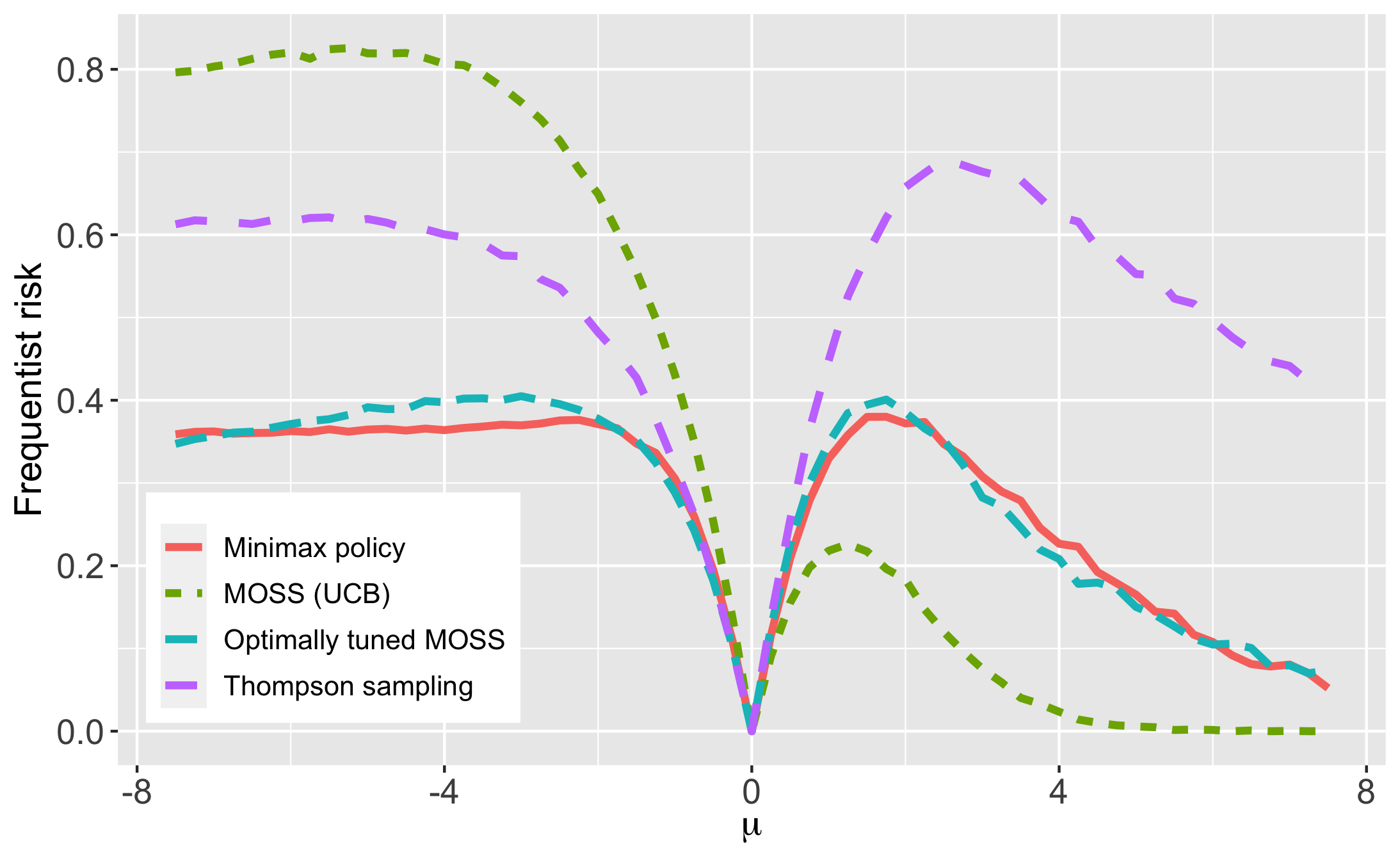
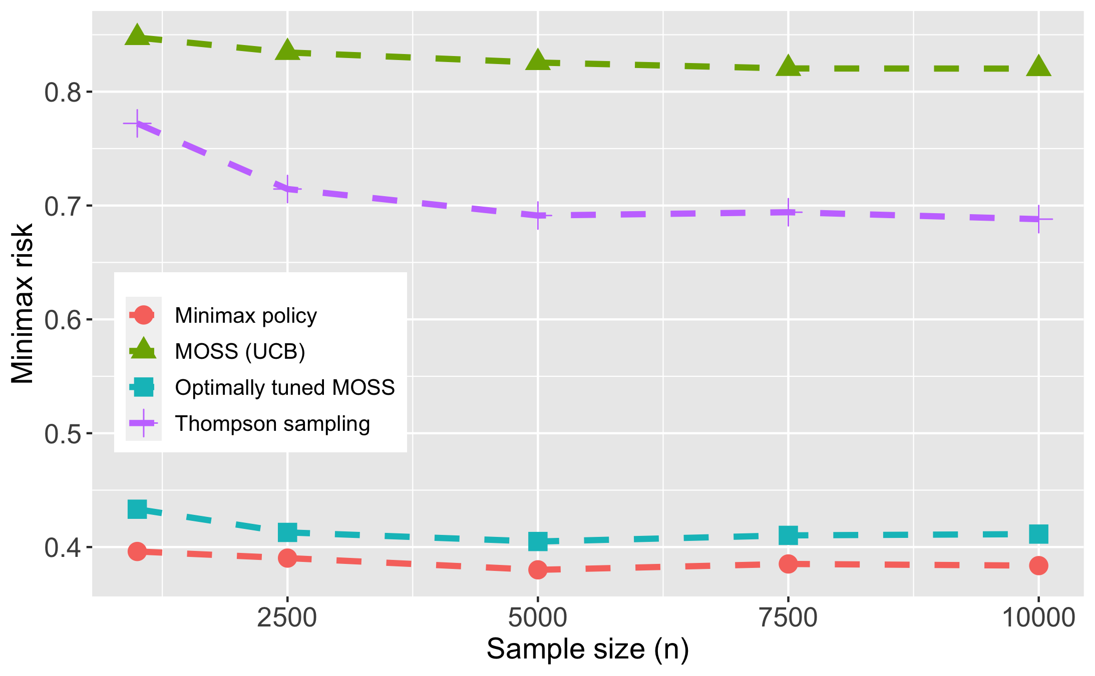
A: Risk profiles of various policies

B: Minimax risk vs n

Note: Panel A shows the frequentist risk profiles of various policies under $n=5000$. The x-axis represents the scaled mean $\mu=(p-p_{0})\cdot\sqrt{p_{0}(1-p_{0})/n}$ with $p_{0}=0.05$. Panel B shows how the minimax risk of the various policies changes with $n$. For reference, the minimax lower bound is $0.373$.

Figure 6.1. Empirical illustration - one-armed bandit

6.3. Two-armed bandits

The second illustration is based on experiments conducted by The Washington Post for selecting between two different images for the headline of a news article. The goal was to choose the one with the highest click-through rate (CTR). Let $p_{0},p_{1}$ denote the CTRs for the two proposals. For this illustration we employ a Bayesian approach with an independent Gaussian prior $p_{k}\sim\mathcal{N}(p_{\textrm{ref}},\sigma_{\textrm{ref}}^{2}\nu^{2}/n)$ for $k\in\{0,1\}$, where $\sigma_{\textrm{ref}}:=p_{\textrm{ref}}(1-p_{\textrm{ref}})$ and $n$ is the number of periods of experimentation. In practice, one would like to set $p_{\textrm{ref}}$ and $\nu^{2}$ based on prior knowledge of the distribution of CTRs across all the news articles. In the absence of this information, we set $p_{\textrm{ref}}=0.175$, which is a typical CTR for media websites, along with $\nu=5$ and vary $n$ between $1000$ and $5000$. When $n=2500$, our choice implies that the 95% range for the prior is $[0.1,0.25]$. For comparison, in the Washington Post study, the actual CTRs turned out to be $0.117$ and $0.246$. Let $\tilde{Y}^{(k)}\sim\textrm{Bernoulli}(p_{k})$ denote the outcomes (i.e., clicks) under option $k\in\{0,1\}$; for convenience, we rescale them to $Y^{(k)}=(\tilde{Y}^{(k)}-p_{\textrm{ref}})/\sigma_{\textrm{ref}}$. The corresponding score processes are then $x_{nq}^{(k)}=n^{-1/2}\sum_{i=1}^{\left\lfloor nq\right\rfloor}Y_{i}^{(k)}$.

The set of algorithms considered are the optimal Bayes algorithm, TS (with the Gaussian prior) and MOSS with both the textbook and tuned implementations. For the tuned version, we set the tuning parameter to the value that minimizes Bayes risk. Figure 6.2, Panel A plots the Bayes risk of these policies under different $n$. As in the first illustration, while the risk of TS and the standard MOSS algorithm is substantially worse that that of the optimal Bayes policy, the optimally tuned MOSS comes within $15\%$ of the lower bound on risk. The actual Washington Post study employed a standard UCB algorithm without any tuning; this performs even worse than MOSS. Panel B of the same figure plots the frequentist risk profiles of these policies under $(p_{0},p_{1})=(p_{\textrm{ref}}-\mu\sigma_{\textrm{ref}}/\sqrt{n},p_{\textrm{ref}}+\mu\sigma_{\textrm{ref}}/\sqrt{n})$, with $n=3000$, and as we vary $\mu$ between 0 and $10$. Setting $\mu=10$ gives a value of $(p_{0},p_{1})$ that is roughly the same as that actually observed in the Washington Post study. Atleast for this class of mean reward values, it is seen that the optimal Bayes policy uniformly dominates all the existing algorithms.

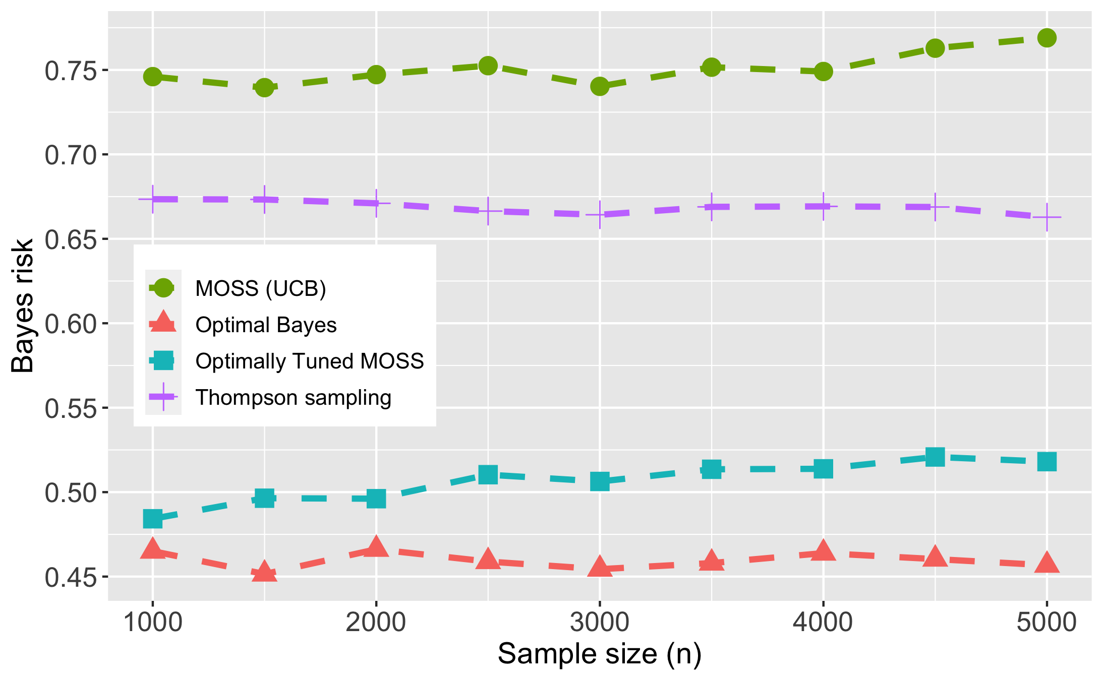
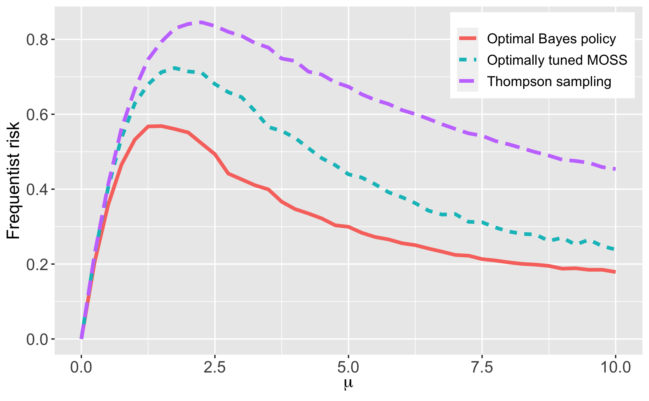
A: Bayes risk vs n

B: Frequentist risk profiles

Note: Panel A shows the Bayes risk of the different algorithms under various values of $n$. Panel B shows the risk profiles of the various policies under $(p_{0},p_{1})\equiv(p_{\textrm{ref}}-\mu\sigma_{\textrm{ref}}/\sqrt{n},p_{\textrm{ref}}+\mu\sigma_{\textrm{ref}}/\sqrt{n})$ when $n=3000$, and we we vary $\mu$ between $0$ and $10$.

Figure 6.2. Empirical illustration - two-armed bandits

6.3.1. Implementation details for the Monte-Carlo algorithm

We employ Algorithm 1 with $B=2000$ and $\Delta t=0.01$. The unbiased estimate, $y_{b}^{(k)}$, is obtained by simulating $\hat{V}_{j+1}^{*}\left(\left\{x_{b,j}^{(l)}+\Delta x_{b,j}^{(l)},q_{b,j}^{(l)}+\Delta q_{b,j}^{(l)}\right\}_{l=0}^{K-1}\right)$ 50 times, and averaging the results. For the prediction model, we employ Random Forest (RF) as it is relatively insensitive to tuning parameter selection. As an alternative, MARS (multivariate adaptive regression splines) delivers essentially the same results, but requires more fine-tuning. In running the RF algorithm, we find that better predictive performance (in terms of achieving lower prediction error with fewer $B$) could be achieved by using $\{\mu^{(k)}(s(t)),q^{(k)}(s(t))\}_{k},\mu^{\max}(s(t))$ as inputs instead of $\{x^{(k)}(t),q^{(k)}(t)\}_{k}$; the former is of course just a nonlinear transformation of the latter.

7. Conclusion

In this article, we derive sharp lower bounds for Bayes and minimax risk of bandit algorithms under diffusion asymptotics and suggest ways to numerically compute the corresponding optimal policies. Our local asymptotic analysis of Bayes risk is substantially different from existing approaches and is arguably more powerful, as it enables us to rank various policies which were previously were indistinguishable on the basis of their large-deviation regret properties. We show that all bandit problems, be they parametric or non-parametric, are asymptotically equivalent to Gaussian bandits. Furthermore, it is asymptotically sufficient to restrict attention to just two state variables per arm. For minimax risk, the paper only proves a lower bound. While we believe the bound is tight, further work is needed to show this. The work also raises a number of avenues for future research, a few of which are discussed below:

Unknown $\sigma$. A drawback of diffusion asymptotics, and of first-order efficiency criteria more generally, is that replacing unknown variances with consistent estimates has no effect on asymptotic risk. One could in principle achieve optimal risk by (say) sampling all arms equally for $\bar{n}:=n^{\rho}$ periods, $\rho\in(0,1)$, obtaining estimates of $\sigma$, and applying the optimal policies based on those estimates from $\bar{n}$ onwards. But in finite samples, the choice of $\rho$ will matter and further work is needed to choose this efficiently.

Other sequential experiments. Adusumilli (2022a) applies insights from this paper to derive the minimax optimal policy for best-arm identification when there two arms, while Adusumilli (2022b) does the same for the problem of costly sampling.

Appendix A Proofs

A.1. Proof of Theorem 2

For this proof, we make the time change $\tau:=1-t$. Let $s:=(x,q,\tau)$, $\mathbb{I}_{n}\equiv\{\tau<1/n\}$ and denote the domain of $s$ by $\mathcal{S}$. Also, let $C^{\infty}(\mathcal{S})$ denote the set of test functions, i.e., the set of all infinitely differentiable functions $\phi:\mathcal{S}\to\mathbb{R}$ such that $\sup_{q\geq 0}|D^{q}\phi|\leq M$ for some $M<\infty$.

Following the time change, we can alternatively represent the solution, $V_{n}^{*}(\cdot)$, to (3.1) as the solution (over the set of all possible functions $\phi:\mathcal{S}\to\mathbb{R}$) to the approximation scheme

$$S_{n}(s,\phi(s),[\phi]) =0\ \textrm{for $\tau>0$};\quad\phi(x,q,0)=0,$$ (A.1)

where for any $u\in\mathbb{R}$ and $\phi_{2}:\mathcal{S}\to\mathbb{R}$,

$$S_{n}(s,u,[\phi_{2}])$$

$$:=-\min_{\pi\in[0,1]}\left\{\frac{\mu^{+}(s)-\pi\mu(s)}{n}+\mathbb{E}\left[\left.\mathbb{I}_{n}\cdot\phi_{2}\left(x+\frac{A_{\pi}Y_{nq+1}}{\sqrt{n}},q+\frac{A_{\pi}}{n},\tau-\frac{1}{n}\right)-u\right|s\right]\right\}.$$

The notation $[\phi_{2}]$ in $S_{n}(s,u,[\phi_{2}])$ refers to the fact that it is a functional argument. Define

$$F(D^{2}\phi,D\phi,s)=\partial_{\tau}\phi-\mu^{+}(s)-\min\left\{-\mu(s)+L[\phi](s),0\right\},$$

as the left-hand side of PDE (2.8) after the time change. Barles and Souganidis (1991) show that the solution, $V_{n}^{*}(\cdot)$, of (A.1) converges to the solution, $V^{*}(\cdot)$, of $F(D^{2}\phi,D\phi,s)=0$ with the boundary condition $\phi(x,q,0)=0$ if the scheme $S_{n}(\cdot)$ satisfies the properties of monotonicity, stability and consistency.

Monotonicity requires $S_{n}(s,u,[\phi_{1}])\leq S_{n}(s,u,[\phi_{2}])$ for all $s\in\mathcal{S}$, $u\in\mathbb{R}$ and $\phi_{1}\geq\phi_{2}$. This is clearly satisfied.

Stability requires (A.1) to have a unique solution, $V_{n}^{*}(\cdot)$, that is uniformly bounded. That a unique solution exists follows from backward induction. To obtain an upper bound, note that following a state $s$, the DM may choose to pull the arm in all subsequent periods. This results in a risk of $\tau\left(\mu^{+}(s)-\mu(s)\right)$. Alternatively, if DM chooses not to pull the arm in all subsequent periods, the resulting risk is $\tau\mu^{+}(s)$. Hence, by definition of $V_{n}^{*}(\cdot)$ as the risk under an optimal policy,

$$0\leq V_{n}^{*}(s)\leq\tau\min\left\{\mu^{+}(s)-\mu(s),\mu^{+}(s)\right\}\leq C\tau.$$ (A.2)

Finally, consistency requires that for all $\phi\in C^{\infty}(\mathcal{S})$, and $s\equiv(x,q,\tau)\in\mathcal{S}$ such that $\tau>0$,

$$\limsup_{\begin{subarray}{c}n\to\infty\\ \rho\to 0\\ z\to s\end{subarray}}nS_{n}(z,\phi(z)+\rho,[\phi+\rho]) \leq F(D^{2}\phi(s),D\phi(s),s),\textrm{ and }$$ (A.3)

$$\liminf_{\begin{subarray}{c}n\to\infty\\ \rho\to 0\\ z\to s\end{subarray}}nS_{n}(z,\phi(z)+\rho,[\phi+\rho]) \geq F(D^{2}\phi(s),D\phi(s),s).$$ (A.4)

It suffices to restrict attention to $\tau>0$ because (A.2) implies that for any $s$ on the boundary, i.e., of the form $(x,q,0)$,

$$\limsup_{\begin{subarray}{c}n\to\infty\\ z\to s\end{subarray}}V_{n}^{*}(z)=0=\liminf_{\begin{subarray}{c}n\to\infty\\ z\to s\end{subarray}}V_{n}^{*}(z).$$

When the above holds, an analysis of the proof of Barles and Souganidis (1991, Theorem 2.1) shows that we only need prove (A.3) and (A.4) for interior values of $s$, i.e., when $\tau>0$.

We now show (A.3). The argument for (A.4) is similar. Since any $z\equiv(\tilde{x},\tilde{q},\tilde{\tau})$ converging to $s\equiv(x,q,\tau)$ with $\tau>0$ will eventually satisfy $\tilde{\tau}>1/n$, we can drop $\mathbb{I}_{n}$ in the definition of $S_{n}(\cdot)$ while taking the $\limsup$ operation in (A.3). Now, for any $s\in\mathcal{S}$, a third order Taylor expansion gives

$$n\mathbb{E}\left[\left.\phi\left(x+\frac{\mathbb{I}(A_{\pi}=1)Y_{nq+1}}{\sqrt{n}},q+\frac{\mathbb{I}(A_{\pi}=1)}{n},\tau-\frac{1}{n}\right)-\phi(s)\right|s\right]$$

$$=\mathbb{E}\left[\left.\sqrt{n}\mathbb{I}(A_{\pi}=1)Y_{nq+1}\right|s\right]\partial_{x}\phi+\frac{1}{2}\mathbb{E}\left[\left.\mathbb{I}(A_{\pi}=1)Y_{nq+1}^{2}\right|s\right]\partial_{x}^{2}\phi$$

$$\qquad+\mathbb{E}\left[\left.\mathbb{I}(A_{\pi}=1)\right|s\right]\partial_{q}\phi-\partial_{\tau}\phi+\frac{R(s)}{\sqrt{n}}$$

where $R(s)$ is a continuous function of $\mu(s)$, $\mathbb{E}\left[\left.\mu{}^{2}\right|s\right]$ and $\mathbb{E}\left[\left.|Y_{nq+1}|^{3}\right|s\right]$ that is bounded at each $s$ as long as these three functions are also bounded. Because $A_{\pi}\sim\textrm{Bernoulli}(\pi)$ for any given $\pi\in[0,1]$, we have $\mathbb{E}\left[\left.\sqrt{n}\mathbb{I}(A_{\pi}=1)Y_{nq+1}\right|s\right]=\pi\mu(s)$, $\mathbb{E}\left[\left.\mathbb{I}(A_{\pi}=1)Y_{nq+1}^{2}\right|s\right]=\pi(\sigma^{2}+n^{-1}\mathbb{E}[\mu^{2}|s])$ and $\mathbb{E}\left[\left.\mathbb{I}(A_{\pi}=1)\right|s\right]=\pi$. Furthermore, recalling that $Y|\mu\sim\mathcal{N}(\mu/\sqrt{n},\sigma^{2})$, the properties of the Gaussian distribution imply

$$\mathbb{E}\left[\left.|Y_{nq+1}|^{3}\right|s\right]=\mathbb{E}\left[\left.\mathbb{E}\left[|Y_{nq+1}|^{3}|\mu\right]\right|s\right]\apprle n^{-3/2}\mathbb{E}\left[\left.|\mu|^{3}\right|s\right]<\infty$$

under the stated assumptions. Based on the above, we obtain

$$nS_{n}(z,\phi(z)+\rho,[\phi+\rho])$$

$$=-\min_{\pi\in[0,1]}\left\{\left(\mu^{+}(z)-\pi\mu(z)\right)+\pi L[\phi](z)-\partial_{\tau}\phi(z)+\frac{R(z)}{\sqrt{n}}+\partial_{x}^{2}\phi(z)\frac{\mathbb{E}[\mu^{2}|z]}{n},0\right\}$$

$$\leq-\min_{\pi\in[0,1]}\left\{\left(\mu^{+}(z)-\pi\mu(z)\right)+\pi L[\phi](z)-\partial_{\tau}\phi(z),0\right\}+\frac{|R(z)|}{\sqrt{n}}+\frac{M\mathbb{E}[\mu^{2}|z]}{n}$$

$$=\partial_{\tau}\phi(z)-\mu^{+}(z)-\min\left\{-\mu(z)+L[\phi](z),0\right\}+\frac{|R(z)|}{\sqrt{n}}+\frac{M\mathbb{E}[\mu^{2}|z]}{n}.$$

Because $\limsup_{z\to s}\{|R(z)|+\mathbb{E}[\mu^{2}|z]\}<\infty$, $\phi\in C^{\infty}(\mathcal{S})$ and $\mu^{+}(\cdot),\mu(\cdot)$ are continuous functions,

$$\limsup_{\begin{subarray}{c}n\to\infty\\ \rho\to 0\\ z\to s\end{subarray}}nS_{n}(z,\phi(z)+\rho,[\phi+\rho])$$

$$\leq\limsup_{\begin{subarray}{c}z\to s\end{subarray}}\partial_{\tau}\phi(z)-\mu^{+}(z)-\min\left\{-\mu(z)+L[\phi](z),0\right\}$$

$$=F(D^{2}\phi(s),D\phi(s),s).$$

This completes the proof of consistency.

A.2. Proof of Theorem 4

For this proof, we use $|f|$ to represent the sup norm of $f$. Let $V_{\Delta t,n,l}^{*}(x,q)$ denote the Bayes risk in the fixed $n$ setting at state $(x,q,t_{L-l})$ under $\pi_{\Delta t}^{*}(\cdot).$ Then $V_{\Delta t,0}^{*}(x,q)=0,$ and $V_{\Delta t,n,l+1}^{*}(\cdot)$ satisfies

$$V_{\Delta t,n,l+1}^{*}(x,q) =\tilde{\Gamma}_{\Delta t}\left[V_{\Delta t,n,l}^{*}\right](x,q);\ l=0,\dots,L-1,\ \textrm{where}$$ (A.5)

$$\tilde{\Gamma}_{\Delta t}[\phi](x,q) :=\min\left\{\tilde{S}_{\Delta t}\left[\phi\right](x,q),\phi(x,q)+\Delta t\cdot\mu^{+}(x,q)\right\},$$

and $\tilde{S}_{\Delta t}\left[\phi\right](x,q)$ denotes the solution at $(x,q,\Delta t)$ of the recursive equation

$$f\left(x,q,\tau\right) =\mathbb{E}\left[\left.\frac{\mu^{+}(x,q)-\mu(x,q)}{n}+f\left(x+\frac{Y}{\sqrt{n}},q+\frac{1}{n},\tau-\frac{1}{n}\right)\right|s\right];\ \tau>0$$

$$f\left(x,q,0\right) =\phi(x,q).$$ (A.6)

In other words, $\tilde{S}_{\Delta t}\left[\phi\right](x,q)$ is the discrete time counterpart of the operator $S_{\Delta t}[\cdot]$ defined in Section 3.3.

For any $k>0$, it can be seen from the recursive definitions of $V_{\Delta t,n,l}^{*}$ and $V_{\Delta t,l}^{*}$,

$$|V_{\Delta t,n,l+1}^{*}-V_{\Delta t,l+1}^{*}| \leq\left|\tilde{\Gamma}_{\Delta t}\left[V_{\Delta t,n,l}^{*}\right]-\tilde{\Gamma}_{\Delta t}\left[V_{\Delta t,l}^{*}\right]\right|+\left|\tilde{S}_{\Delta t}\left[V_{\Delta t,l+1}^{*}\right]-S_{\Delta t}\left[V_{\Delta t,l+1}^{*}\right]\right|.$$

Recall that $\tilde{S}_{\Delta t}\left[\phi\right]$ denotes the solution to (A.6), while $S_{\Delta t}[\phi]$ denotes the solution to (3.3), when the initial condition in both cases is $\phi$. Hence, by Barles and Jakobsen (2007, Theorem 3.1), the regularity conditions of which can be verified as in Appendix B, we have $\left|\tilde{S}_{\Delta t}\left[V_{\Delta t,l+1}^{*}\right]-S_{\Delta t}\left[V_{\Delta t,l+1}^{*}\right]\right|\lesssim n^{-1/14}$. Additionally, it is straightforward to verify $\left|\tilde{\Gamma}_{\Delta t}\left[\phi_{1}\right]-\tilde{\Gamma}_{\Delta t}\left[\phi_{2}\right]\right|\leq|\phi_{1}-\phi_{2}|$ for all $\phi_{1},\phi_{2}$. Together, these results imply

$$|V_{\Delta t,n,l+1}^{*}-V_{\Delta t,l+1}^{*}|\lesssim|V_{\Delta t,n,l}^{*}-V_{\Delta t,l}^{*}|+n^{-1/14}\lesssim l\cdot n^{-1/14},$$

where the last inequality follows by iterating on $l$. Since $L$ is finite under a fixed $\Delta t$, we have thereby shown $\lim_{n\to\infty}|V_{\Delta t,n,l+1}^{*}-V_{\Delta t,l+1}^{*}|=0$ for all $l=0,\dots,L-1$. The claim follows by combining this result with Theorem 3.

A.3. Proof outline of Theorem 5

​​​ We may suppose without loss of generality that $\Pi$ consists only of deterministic policies as this restriction is immaterial for Bayes risk. We start by writing $V_{\pi,n}(0)$ in a convenient form. The regret payoff (2.2) can be expanded as

$$R(Y,\pi,h)=\frac{\mu_{n}(h)}{\sqrt{n}}\left\{\mathbb{I}(\mu_{n}(h)\geq 0)-\pi\right\}+\frac{\epsilon}{\sqrt{n}}\left\{\mathbb{I}(\mu_{n}(h)\geq 0)-\pi\right\},$$

where $\epsilon:=Y-\mu_{n}(h)$ is mean $0$ conditional on $\pi,h$ (we have used $\pi$ in place of $A$ as they are equivalent for deterministic policies). Set

$$R_{n}(h,\pi):=n\mathbb{E}\left[R(Y_{j},\pi_{j},h)|\pi_{j},h\right]=\sqrt{n}\mu_{n}(h)\left\{\mathbb{I}(\mu_{n}(h)\geq 0)-\pi\right\}.$$

Now, $\pi_{j+1}$ is a deterministic function of ${\bf y}_{nq_{j}(\pi)}$ for deterministic policies. Then, by the definition of $V_{\pi,n}(0)$ given in Section 4.2, and the law of iterated expectations,

$$V_{\pi,n}(0) =\mathbb{E}_{({\bf y}_{n},h)}\left[\frac{1}{n}\sum_{j=1}^{n}R_{n}(h,\pi_{j})\right]=\bar{\mathbb{E}}_{n}\left[\frac{1}{n}\sum_{j=0}^{n-1}\mathbb{E}\left[\left.R_{n}(h,\pi_{j+1})\right|{\bf y}_{nq_{j}(\pi)}\right]\right],$$ (A.7)

where we write $q_{j}(\pi)$ to make explicit the dependence of $q_{j}$ on the policy $\pi$.

In Section 4.1, we used the approximate likelihood $\Lambda_{n,h}({\bf y}_{n})$ to obtain an approximation, $\tilde{p}_{n}(\cdot|{\bf y}_{nq})\equiv\tilde{p}_{n}(\cdot|x_{nq},q)$, to the true posterior density. In a similar vein, we can approximate the true marginal density, $d\bar{P}_{n}({\bf y}_{n}):=\int p_{n,\theta_{0}+h/\sqrt{n}}({\bf y}_{n})\cdot m_{0}(h)d\nu(h)$, with $d\tilde{\bar{P}}_{n}({\bf y}_{n}):=\int d\Lambda_{n,h}({\bf y}_{n})\cdot m_{0}(h)d\nu(h)$. Let $\tilde{\mathbb{E}}[\cdot|{\bf y}_{nq}]$, $\tilde{\mathbb{E}}_{n}[\cdot]$ denote the expectations corresponding to $\tilde{p}_{n}(\cdot|{\bf y}_{nq})$ and $d\tilde{\bar{P}}_{n}$. Define $\tilde{V}_{\pi,n}(0)$ as the quantity obtained by replacing the inner and outer expectations in (A.7) with their approximations $\tilde{\mathbb{E}}[\cdot|{\bf y}_{nq}]$ and $\tilde{\mathbb{E}}_{n}[\cdot]$, i.e.,

$$\tilde{V}_{\pi,n}(0):=\tilde{\mathbb{E}}_{n}\left[\frac{1}{n}\sum_{j=0}^{n-1}\tilde{\mathbb{E}}\left[\left.R_{n}(h,\pi_{j+1})\right|{\bf y}_{nq_{j}(\pi)}\right]\right].$$ (A.8)

From the SLAN property (4.2), we can show that $\tilde{p}_{n}(\cdot|{\bf y}_{nq}),\tilde{\bar{P}}_{n}({\bf y}_{n})$ converge uniformly over $q$ in the total-variation metric to $p_{n}(\cdot|{\bf y}_{nq}),\bar{P}_{n}({\bf y}_{n})$; see D.1-D.4 in Appendix D for the precise claim. This in turn implies that

$$\lim_{n\to\infty}\sup_{\pi\in\Pi}\left|V_{\pi,n}(0)-\tilde{V}_{\pi,n}(0)\right|=0.$$ (A.9)

Now, $\tilde{\bar{P}}_{n}$ is not a probability measure, even as it integrates to 1 asymptotically. We therefore modify $\tilde{\mathbb{E}}_{n}[\cdot]$ slightly to make it a ‘true’ expectation, leading to another approximation, $\breve{V}_{\pi,n}(0)$, of $\tilde{V}_{\pi,n}(0)$, such that $\lim_{n\to\infty}\sup_{\pi\in\Pi}\left|\breve{V}_{\pi,n}(0)-\tilde{V}_{\pi,n}(0)\right|=0$ (see step 2 in Appendix D). Following this adjustment and using dynamic-programming, the optimization problem $\inf_{\pi\in\Pi}\breve{V}_{\pi,n}(0)$ can written in a recursive form akin to (3.1), see (D.12) in Appendix D. Inspection of this recursive form shows $\inf_{\pi\in\Pi}\breve{V}_{\pi,n}(0)=\inf_{\pi\in\Pi^{\mathcal{S}}}\breve{V}_{\pi,n}(0)$. Intuitively, this is because $\tilde{\mathbb{E}}[\cdot|{\bf y}_{nq}]$ is a function only of $x_{nq},q$, while $\Lambda_{n,h}({\bf y}_{n})$, which was used to define the approximate marginal $\tilde{\bar{P}}_{n}({\bf y}_{n})$, has a similar form to a Gaussian likelihood that depends only on $x_{nq},q$ as well. This proves the first claim. For the second claim, similar arguments as in the proof of Theorem 2 show that the solution to the recursive problem converges to the solution of PDE (2.8).

For the last claim, observe that (A.9) also implies $\lim_{n\to\infty}V_{\pi_{\Delta t}^{*},n}(0)-\tilde{V}_{\pi_{\Delta t}^{*}n}(0)=0$. We then approximate $\tilde{V}_{\pi_{\Delta t}^{*}n}(0)$ with $\breve{V}_{\pi_{\Delta t}^{*}n}(0)$, write the latter again in recursive form, and argue as in the proof of Theorem 4 that $\lim_{n\to\infty}|\breve{V}_{\pi_{\Delta t}^{*}n}(0-V^{*}(0)|\lesssim\Delta t{}^{1/4}$.

Supplementary appendix

Appendix B Rates of convergence to the PDE solution

The results of Barles and Jakobsen (2007, Theorem 3.1) provide a bound on the rate of convergence of $V_{n}^{*}(\cdot)$ to $V^{*}(\cdot)$. The technical requirements to obtain this are described in their Assumptions A2 and S1-S3. Assumptions A2 and S1-S2 are straightforward to verify using the regularity conditions given for Theorem 2 with the additional requirement $\sup_{s}|\mu^{+}(s)|<\infty$.

Assumption S3 of Barles and Jakobsen (2007) is a strengthening of the consistency requirement in (A.3) and (A.4). Suppose that the test function $\phi\in\mathcal{C}^{\infty}(\mathcal{S})$ is such that $\left|\partial_{t}^{\beta_{0}}D_{(x,q)}^{\beta}\phi(x,q,t)\right|\leq K\varepsilon^{1-2\beta_{0}-\left\|\beta\right\|}$ for all $\beta_{0}\in\mathbb{N},\beta\in\mathbb{N}\times\mathbb{N}$. Then by a third order Taylor expansion as in the proof of Theorem 2 and some tedious but straightforward algebra,

$$\left|nS_{n}(z,\phi(z)+\rho,[\phi+\rho])-F(D^{2}\phi(s),D\phi(s),s)\right|\leq E(n,\varepsilon)\equiv\frac{\bar{K}}{n^{1/2}\varepsilon^{2}},$$

where $\bar{K}$ depends only on $K$, defined above, and the upper bounds on $\mu^{+}(\cdot),\mu(\cdot)$. The above suffices to verify the Assumption S3 of Barles and Jakobsen (2007); note that the definition of $S(\cdot)$ in that paper is equivalent to $nS_{n}(\cdot)$ here.

Under the above conditions, Barles and Jakobsen (2007, Theorem 3.1) implies

$$V^{*}-V_{n}^{*} \apprle\sup_{\varepsilon}\left(\varepsilon+E(n,\varepsilon)\right)\apprle n^{-1/6}\ \textrm{and }$$

$$V_{n}^{*}-V^{*} \apprle\sup_{\varepsilon}\left(\varepsilon^{1/3}+E(n,\varepsilon)\right)\apprle n^{-1/14}.$$ (B.1)

The asymmetry of the rates is an artifact of the techniques of Barles and Jakobsen (2007). The rates are also far from optimal. The results of Barles and Jakobsen (2007), while being relatively easy to apply, do not exploit any regularity properties of the approximation scheme. There do sexist approximation schemes for PDE (2.8) that converge at the faster $n^{-1/2}$ rates. While it is unknown whether (3.1) is one of them, we do find that in practice the quality of approximation of $V^{*}$ with $V_{n}^{*}$ is far better than what (B.1) appears to suggest; the Monte-Carlo simulation in Figure B.1 attests to this (the simulation employs a normal prior $\mu\sim\mathcal{N}(0,50^{2})$ with $\sigma=5$).

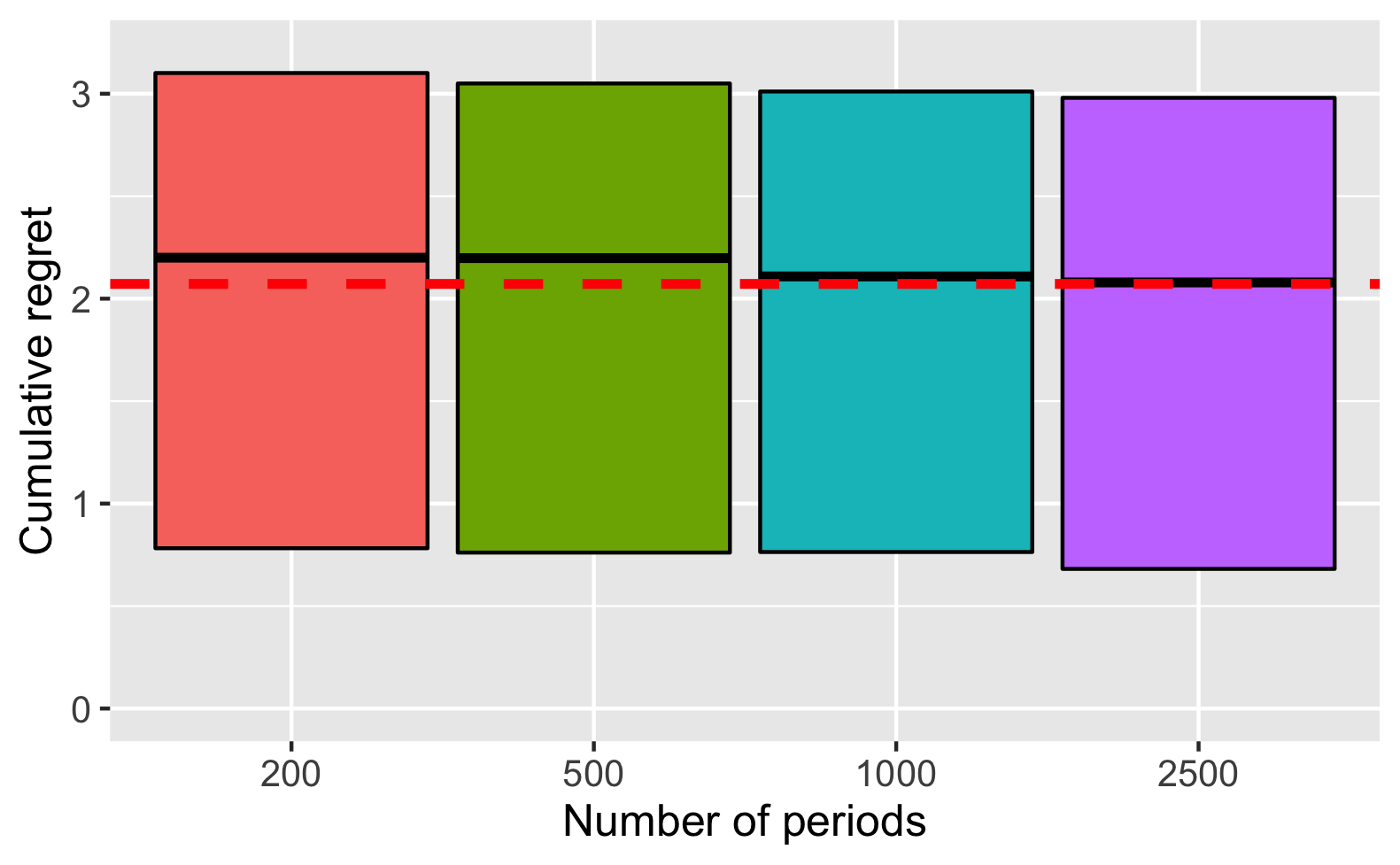
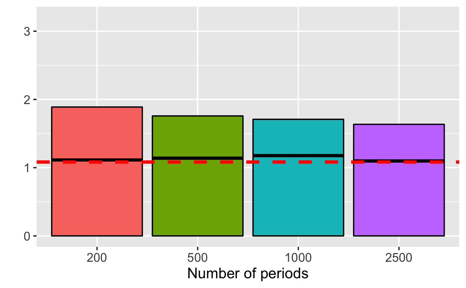
A: Thompson sampling

B: Optimal Bayes policy

Note: The parameter values are $\mu_{0}=0$, $\nu=50$ and $\sigma=5$. The dashed red lines denote the values of asymptotic Bayes risk. Black lines within the bars denote the Bayes risk in finite samples. The bars describe the interquartile range of regret.

Figure B.1. Monte-Carlo simulations

Appendix C Lower bounds on minimax risk

Recall the definition of $V_{n,\pi}(0;h)$ from Section 4.4 as the frequentist risk under some $\pi\in\Pi$. We also make the dependence of $V_{n}^{*}(0),V^{*}(0)$ on the priors $m_{0}$ explicit by writing them as $V_{n}^{*}(0;m_{0}),V^{*}(0;m_{0})$. Clearly, $\inf_{\pi\in\Pi}\sup_{|h|\leq\Gamma}V_{n,\pi}(0;h)\geq V_{n}^{*}(0;m_{0})$ for any prior $m_{0}$ supported on $|h|\leq\Gamma$. So, Theorem 5 implies

$$\lim_{n\to\infty}\inf_{\pi\in\Pi}\sup_{|h|\leq\Gamma}V_{n,\pi}(0;h)\geq\sup_{m_{0}\in\mathcal{P}}V^{*}(0;m_{0})$$

where $\mathcal{P}$ is the set of all compactly supported distributions. We now claim that

$$\sup_{m_{0}\in\mathcal{P}}V^{*}(0;m_{0})=\bar{V}^{*},$$ (C.1)

where $\bar{V}^{*}$ is the asymptotic minimax risk in the Gaussian setting. The above is easily shown for scalar $\theta$ by transforming the state variable $x$ to $\dot{\mu}_{0}x$ and replacing $\sigma^{2}$ with $\dot{\mu}_{0}^{2}\sigma^{2}$, following which the infinitesimal generator (4.6) becomes equivalent to the one in (2.8) since $\mu(s)=\dot{\mu}_{0}h(s)$. The argument for vector $\theta$ is given below.

C.0.1. Proof of (C.1) for vector $\theta$

We employ the same notation as in Section 4.3. It is without loss of generality to suppose $\Sigma=I$, otherwise, we can perform the subsequent analysis after applying the transformations $h\leftarrow\Sigma^{-1/2}h,x\leftarrow\Sigma^{-1/2}x$ and $\dot{\mu}_{0}\leftarrow\Sigma^{1/2}\dot{\mu_{0}}$. Consider the class, $\bar{\mathcal{P}}$, of priors, $m_{0}$, over $h$ supported on $\mu\cdot\dot{\mu}_{0}/(\dot{\mu}_{0}^{\intercal}\mu_{0})$, where $\mu\in\mathbb{R}$ can take on various values (so $m_{0}$ is, in essence, a prior on $\mu$). For these priors, $\dot{\mu}_{0}^{\intercal}h=\mu$. Recall that under the approximate posterior, $\tilde{p}_{n}(h|x,q)\propto\mathcal{N}(x|qh,q\Sigma)\cdot m_{0}(h)$. It is then easily verified that, for the class $\bar{\mathcal{P}}$, $\tilde{p}_{n}(h|x,q)$ depends on $x$ only through $\dot{\mu}_{0}^{\intercal}x$. Furthermore, we also have $h(s)=\mu(s)\cdot\dot{\mu}_{0}/(\dot{\mu}_{0}^{\intercal}\mu_{0})$, where $\mu(s),h(s)$ are the posterior means of $\mu,h$ under $\tilde{p}_{n}(\cdot|x,q)$.

Choose $\{\phi_{i}\}_{i=1}^{d-1}$ such that $\{\dot{\mu}_{0}/\dot{\mu}_{0}^{\intercal}\mu_{0},\phi_{1},\dots,\phi_{d-1}\}$ are orthonormal and span $\mathbb{R}^{d}$. Suppose we transform the state variables $x$ to $z$ as $z=Px$, where $P^{\intercal}=[\dot{\mu}_{0},\phi_{1},\dots,\phi_{d-1}]$. Clearly, $P$ is invertible, and the first component of $z$ is $\bar{x}:=\dot{\mu}_{0}^{\intercal}x$. Consider the generator $L[\cdot]$ in (4.7). Following the transformation of variables,

$$h(s)^{\intercal}D_{x}f =\frac{\mu(s)}{\dot{\mu}_{0}^{\intercal}\dot{\mu}_{0}}\dot{\mu}_{0}^{\intercal}\cdot P^{\intercal}D_{z}f=\mu(s)\cdot\left[1,\bm{0}_{1\times(d-1)}\right]\cdot D_{z}f=\mu(s)\partial_{\bar{x}}f,$$

and $\textrm{Tr}\left[D_{x}^{2}f\right]=\textrm{Tr}\left[PP^{\intercal}\cdot D_{z}^{2}f\right]$. Clearly, $PP^{\intercal}$ is block diagonal, with diagonal entries $\dot{\mu}_{0}^{\intercal}\dot{\mu}_{0}$ and $I_{(d-1)}$. Hence, we can write $\textrm{Tr}\left[D_{x}^{2}f\right]=(\dot{\mu}_{0}^{\intercal}\dot{\mu}_{0})\cdot\partial_{\bar{x}}^{2}f+\textrm{Tr}\left[D_{\tilde{x}}^{2}f\right]$ where $\tilde{x}$ is the part of $z$ excluding the first component. Combining the above, and defining $\sigma^{2}:=\dot{\mu}_{0}^{\intercal}\dot{\mu}_{0}$ (more generally, for $\Sigma\neq I$, this would be $\dot{\mu}_{0}^{\intercal}\Sigma\dot{\mu}_{0}$), we have thus shown $L[f](s)=\partial_{q}f+\mu(s)\partial_{\bar{x}}f+\frac{1}{2}\sigma^{2}\partial_{\bar{x}}^{2}f+\frac{1}{2}\textrm{Tr}\left[D_{\tilde{x}}^{2}f\right].$

The minimal Bayes risk, $V^{*}(s;m_{0})$, solves the PDE:

$$\partial_{t}f(s)+\mu^{+}(s)+\min\left\{-\mu(s)+L[f](s),0\right\} =0\ \textrm{if }t<1;\quad f(s)=0\ \textrm{if }t=1.$$

Now, $\tilde{p}_{n}(h|x,q)$ depends on $x$ only though $\bar{x}$, so $\mu(s)\equiv\mathbb{\tilde{E}}[\mu|s],\mu^{+}(s)\equiv\mathbb{\tilde{E}}[\mu\mathbb{I}\{\mu\geq 0\}|s]$ are functions only of $\bar{x},q$. Hence, by similar viscosity solution arguments as in the proof of Theorem 6, it follows that $V^{*}(s;m_{0})$ solves

$$\partial_{t}f(\bar{s})+\mu^{+}(\bar{s})+\min\left\{-\mu(\bar{s})+\bar{L}[f](\bar{s}),0\right\} =0\ \textrm{if }t<1;\quad f(\bar{s})=0\ \textrm{if }t=1,$$

where $\bar{s}:=(\bar{x},q,t)$ and $\bar{L}[f](\bar{s})=\partial_{q}f+\mu(\bar{s})\partial_{\bar{x}}f+\frac{1}{2}\sigma^{2}\partial_{\bar{x}}^{2}f$. But the above has the same form as PDE (2.8) in the Gaussian setting if we interpret $m_{0}$ as a prior on $\mu$. Hence, $\sup_{m_{0}\in\bar{\mathcal{P}}}V^{*}(0;m_{0})=\bar{V}^{*}$, the minimax risk in the Gaussian regime.

Since $\bar{\mathcal{P}}\subset\mathcal{P}$, the set of all compactly supported priors on $\bm{h}$, we have thereby derived a lower bound on minimax risk. As an aside, we note that our proof also goes through after replacing $\bar{\mathcal{P}}$ with the class of product priors defined in Section 5; the argument would then be similar to the proof of Theorem 6, see Appendix F.

Appendix D Proof of Theorem 5

Recall that ${\bf y}_{i}=\{Y_{k}\}_{k=1}^{i}$ denotes the rewards after $i$ pulls of the arms. Denote by $\mathbb{E}_{({\bf y}_{n},h})[\cdot]$ the expectation under the ‘true’ joint density $dS_{n}({\bf y}_{n},h):=\left\{\prod_{i=1}^{n}p_{\theta_{0}+h/\sqrt{n}}(Y_{i})\right\}\cdot m_{0}(h).$ Let $\nu({\bf y}_{n}):=\prod_{i=1}^{n}\nu(Y_{i})$, $p_{n,\theta}({\bf y}_{n}):=\prod_{k=1}^{n}p_{\theta}(Y_{k})$ and $\bar{P}_{n}$ be the probability measure corresponding to the ‘true’ marginal density $d\bar{P}_{n}({\bf y}_{n}):=\int p_{n,\theta_{0}+h/\sqrt{n}}({\bf y}_{n})\cdot m_{0}(h)d\nu(h)$. We use $\bar{\mathbb{E}}_{n}[\cdot]$ to denote its corresponding expectation. As first defined in Appendix D, let $\tilde{\bar{P}}_{n}$ denote the measure (but not necessarily a probability) corresponding to the density $d\tilde{\bar{P}}_{n}({\bf y}_{n}):=\int d\Lambda_{n,h}({\bf y}_{n})\cdot m_{0}(h)d\nu(h)$. In what follows, we denote $d\Lambda_{n,h}({\bf y}_{n})$ by $\lambda_{n,h}({\bf y}_{n})$ for ease of notation, and note that

$$\lambda_{n,h}({\bf y}_{n}):=d\Lambda_{n,h}({\bf y}_{n})\equiv\frac{d\Lambda_{n,h}({\bf y}_{n})}{d\nu({\bf y}_{n})}=\exp\left\{\frac{1}{\sigma^{2}}hx_{n}-\frac{1}{2\sigma^{2}}h^{2}\right\}p_{n,\theta_{0}}({\bf y}_{n}).$$

Finally, $\left\|\cdot\right\|_{\textrm{TV}}$ denotes the total variation metric between two measures.

The proof follows the basic outline established in Appendix D. Recall the expressions for $V_{\pi,n}(0),\tilde{V}_{\pi,n}(0)$ given in (A.7) and (A.8).

Step 1 (Approximation of $V_{\pi,n}(0)$ with $\tilde{V}_{\pi,n}(0)$):

We start by proving some convergence properties of $\tilde{\bar{P}}_{n}$ and $\tilde{p}_{n}(\cdot|{\bf y}_{nq})$ to $\bar{P}_{n}$ and $p_{n}(\cdot|{\bf y}_{nq})$. The proofs here make heavy use of the SLAN property (4.2) established in Lemma 2. Let $A_{n}$ denote the event $\left\{{\bf y}_{n}:\sup_{q}|x_{nq}|\leq M\right\}$. For any measure $P$, define $P\cap A_{n}$ as the restriction of $P$ to the set $A_{n}$. By Lemma 6 in Appendix E, for any $\epsilon>0$ there exists $M<\infty$ such that

$$\lim_{n\to\infty}\bar{P}_{n}\left(A_{n}^{c}\right) \leq\epsilon,$$ (D.1)

$$\lim_{n\to\infty}\left\|\bar{P}_{n}\cap A_{n}-\tilde{\bar{P}}_{n}\cap A_{n}\right\|_{\textrm{TV}} =0,\ \textrm{and}$$ (D.2)

$$\lim_{n\to\infty}\sup_{q}\bar{\mathbb{E}}_{n}\left[\mathbb{I}_{A_{n}}\left\|p_{n}(\cdot|{\bf y}_{nq})-\tilde{p}_{n}(\cdot|{\bf y}_{nq})\right\|_{\textrm{TV}}\right] =0.$$ (D.3)

The measures $\Lambda_{n,h}(\cdot),\tilde{\bar{P}}_{n}(\cdot)$ are not probabilities as they need not integrate to $1$. But Lemma 6 also shows the following: $\Lambda_{n,h}(\cdot),\tilde{\bar{P}}_{n}(\cdot)$ are $\sigma$-finite and contiguous with respect to $P_{n,\theta_{0}}$, and letting $\mathcal{Y}_{n}$ denote the sample space of ${\bf y}_{n}$,

$$\text{$\lim_{n\to\infty}\tilde{\bar{P}}_{n}$($\mathcal{Y}_{n}$)}=1\quad\textrm{and }\lim_{n\to\infty}\tilde{\bar{P}}_{n}(A_{n}^{c})\leq\epsilon.$$ (D.4)

The first result in (D.4) implies that $\tilde{\bar{P}}_{n}$ is almost a probability measure.

Based on the above, we show that

$$\lim_{n\to\infty}\sup_{\pi\in\Pi}\left|V_{\pi,n}(0)-\tilde{V}_{\pi,n}(0)\right|=0$$ (D.5)

by bounding each term in the following expansion:

$$V_{\pi,n}(0)-\tilde{V}_{\pi,n}(0)$$

$$=\bar{\mathbb{E}}_{n}\left[\mathbb{I}_{A_{n}^{c}}\frac{1}{n}\sum_{j=0}^{n-1}\mathbb{E}\left[\left.R_{n}(h,\pi_{j+1})\right|{\bf y}_{nq_{j}(\pi)}\right]\right]+\tilde{\mathbb{E}}_{n}\left[\mathbb{I}_{A_{n}^{c}}\frac{1}{n}\sum_{j=0}^{n-1}\tilde{\mathbb{E}}\left[\left.R_{n}(h,\pi_{j+1})\right|{\bf y}_{nq_{j}(\pi)}\right]\right]$$

$$\quad+\left(\bar{\mathbb{E}}_{n}-\tilde{\mathbb{E}}_{n}\right)\left[\mathbb{I}_{A_{n}}\frac{1}{n}\sum_{j=0}^{n-1}\tilde{\mathbb{E}}\left[\left.R_{n}(h,\pi_{j+1})\right|{\bf y}_{nq_{j}(\pi)}\right]\right]$$

$$\quad+\bar{\mathbb{E}}_{n}\left[\mathbb{I}_{A_{n}}\frac{1}{n}\sum_{j=0}^{n-1}\left\{\mathbb{E}\left[\left.R_{n}(h,\pi_{j+1})\right|{\bf y}_{nq_{j}(\pi)}\right]-\tilde{\mathbb{E}}\left[\left.R_{n}(h,\pi_{j+1})\right|{\bf y}_{nq_{j}(\pi)}\right]\right\}\right].$$ (D.6)

Because of the compact support of the prior, the posteriors $p_{n}(\cdot|{\bf y}_{nq}),\tilde{p}_{n}(\cdot|{\bf y}_{nq})$ are also compactly supported on $|h|\leq\Gamma$ for all $q$. On this set $|R_{n}(h,\pi_{j})|\leq b\Gamma$ for some $b<\infty$ by Assumption 1(iii). The first two quantities in (D.6) are therefore bounded by $b\Gamma\bar{P}_{n}(A_{n}^{c})$ and $b\Gamma\tilde{\bar{P}}_{n}(A_{n}^{c})$. By (D.1) and (D.4), these can be made arbitrarily small by choosing a suitably large $M$ in the definition of $A_{n}$. The third term in (D.6) is bounded by $b\Gamma\left\|\bar{P}_{n}\cap A_{n}-\tilde{\bar{P}}_{n}\cap A_{n}\right\|_{\textrm{TV}}$. By (D.2) it converges to $0$ as $n\to\infty$. The expression within $\{\}$ brackets in the fourth term of (D.6) is smaller than $b\Gamma\left\|p_{n}(\cdot|{\bf y}_{nq_{j}(\pi)})-\tilde{p}_{n}(\cdot|{\bf y}_{nq_{j}(\pi)})\right\|_{\textrm{TV}}$. Hence, by the linearity of expectations, the term overall is bounded (uniformly over $\pi\in\Pi$) by

$$b\Gamma\sup_{q}\bar{\mathbb{E}}_{n}\left[\mathbb{I}_{A_{n}}\left\|p_{n}(\cdot|{\bf y}_{nq})-\tilde{p}_{n}(\cdot|{\bf y}_{nq})\right\|_{\textrm{TV}}\right],$$

which is $o(1)$ because of (D.3). We have thus shown (D.5).

Step 2 (Approximating $V_{n}^{*}(0)$ with a recursive formula):

The measure, $\tilde{\bar{P}}_{n}$ , used in the outer expectation in the definition of $\tilde{V}_{\pi,n}(0)$ is not a probability. This can be rectified as follows: First, note that the density $\lambda_{n,h}(\cdot)$ can be written as

$$\lambda_{n,h}({\bf y}_{n})=\prod_{i=1}^{n}\left\{\exp\left\{\frac{h}{\sqrt{n}}\psi(Y_{i})-\frac{h^{2}}{2\sigma^{2}n}\right\}p_{\theta_{0}}(Y_{i})\right\}=\prod_{i=1}^{n}\tilde{p}_{n}(Y_{i}|h),$$ (D.7)

where

$$\tilde{p}_{n}(Y_{i}|h):=\exp\left\{\frac{h}{\sqrt{n}}\psi(Y_{i})-\frac{h^{2}}{2\sigma^{2}n}\right\}p_{\theta_{0}}(Y_{i}).$$

Using (D.7), Lemma 7 shows that $\tilde{\bar{P}}_{n}$ can be disintegrated as

$$d\tilde{\bar{P}}_{n}({\bf y}_{n}) =\prod_{i=1}^{n}\left\{\int\tilde{p}_{n}(Y_{i}|h)\tilde{p}_{n}(h|{\bf y}_{i-1})d\nu(h)\right\},$$ (D.8)

with $\tilde{p}_{n}(h|{\bf y}_{0}):=m_{0}(h)$. Now define $c_{n,i}:=\int\left\{\int\tilde{p}_{n}(Y_{i}|h)d\nu(Y_{i})\right\}\tilde{p}_{n}(h|{\bf y}_{i-1})d\nu(h)$, and let $\tilde{\mathbb{P}}_{n}$ denote the probability measure

$$\tilde{\mathbb{P}}_{n}({\bf y}_{n}) =\prod_{i=1}^{n}\tilde{\mathbb{P}}_{n}(Y_{i}|{\bf y}_{i-1}),\ \textrm{where}$$

$$d\tilde{\mathbb{P}}_{n}(Y_{i}|{\bf y}_{i-1}) :=\frac{1}{c_{n,i}}\int\tilde{p}_{n}(Y_{i}|h)\tilde{p}_{n}(h|{\bf y}_{i-1})d\nu(h).$$ (D.9)

Note that $c_{n,i}$ is a random (because it depends on ${\bf y}_{i-1}$) integration factor ensuring $\tilde{\mathbb{P}}_{n}(y_{i+1}|{\bf y}_{i})$, and therefore $\tilde{\mathbb{P}}_{n}$, is a probability. In Lemma 8, it is shown that there exists some non-random $C<\infty$ such that

$$\sup_{i}|c_{n,i}-1|\leq Cn^{-c}\ \textrm{for any }c<3/2,$$ (D.10)

and furthermore, $\left\|\tilde{\mathbb{P}}_{n}-\tilde{\bar{P}}_{n}\right\|_{\textrm{TV}}\to 0$ as $n\to\infty$. Hence, letting

$$\breve{V}_{\pi,n}(0):=\mathbb{E}_{\tilde{\mathbb{P}}_{n}}\left[\frac{1}{n}\sum_{j=0}^{n-1}\tilde{\mathbb{E}}\left[\left.R_{n}(h,\pi_{j+1})\right|{\bf y}_{nq_{j}(\pi)}\right]\right],$$

where $\mathbb{E}_{\tilde{\mathbb{P}}_{n}}[\cdot]$ is the expectation with respect to $\tilde{\mathbb{P}}_{n}$, one obtains the approximation

$$\sup_{\pi\in\Pi}\left|\tilde{V}_{\pi,n}(0)-\breve{V}_{\pi,n}(0)\right|\leq b\Gamma\left\|\tilde{\mathbb{P}}_{n}-\tilde{\bar{P}}_{n}\right\|_{\textrm{TV}}\to 0.$$ (D.11)

See the arguments following (D.6) for the definition of $b$.

Since $\tilde{p}_{n}(h|{\bf y}_{i-1})\equiv\tilde{p}_{n}(h|x=x_{i-1},q=(i-1)/n)$ by (4.5) with $\tilde{p}_{n}(h|x=0,q=0):=m_{0}(h)$, it follows from (D.9) that $\tilde{\mathbb{P}}_{n}(Y_{i}|{\bf y}_{i-1})\equiv\tilde{\mathbb{P}}_{n}(Y_{i}|x=x_{i-1},q=(i-1)/n)$.

Define $\breve{V}_{n}^{*}(0)=\inf_{\pi\in\Pi}\breve{V}_{\pi,n}(0)$. Recall that for a given $\pi\in\{0,1\}$, $\tilde{\mathbb{E}}\left[\left.R_{n}(h,\pi)\right|{\bf y}_{nq_{j}}\right]\equiv\tilde{\mathbb{E}}\left[\left.R_{n}(h,\pi)\right|x_{nq_{j}},q_{j}\right]$ by (4.5). Furthermore, we have noted above that the conditional distribution of the future values of the rewards, $\tilde{\mathbb{P}}_{n}(Y_{nq_{j}+1}|{\bf y}_{nq_{j}})$, also depends only on $(x_{nq_{j}},q_{j})$. Based on this, standard backward induction/dynamic programming arguments imply $\breve{V}_{n}^{*}(0)$ can be obtained as the solution at $(x,q,t)=(0,0,0)$ of the recursive problem

$$\breve{V}_{n}^{*}\left(x,q,t\right) =\min_{\pi\in\{0,1\}}\left\{\frac{\tilde{\mathbb{E}}\left[\left.R_{n}(h,\pi)\right|x,q\right]}{n}+\mathbb{E}_{\tilde{\mathbb{P}}_{n}}\left[\left.\mathbb{I}_{n}\cdot\breve{V}_{n}^{*}\left(x+\frac{\pi\sigma^{2}\psi(Y_{nq+1})}{\sqrt{n}},q+\frac{\pi}{n},t+\frac{1}{n}\right)\right|s\right]\right\};$$

$$\quad\textrm{if }t<1,$$

$$\breve{V}_{n}^{*}\left(x,q,1\right) =0,$$ (D.12)

where $\mathbb{E}_{\tilde{\mathbb{P}}_{n}}\left[\left.\cdot\right|s\right]$ denotes the expectation under $\tilde{\mathbb{P}}_{n}(Y_{nq+1}|{\bf y}_{nq})\equiv\tilde{\mathbb{P}}_{n}(Y_{nq+1}|x=x_{nq},q)$ and $\mathbb{I}_{n}=\mathbb{I}\{t\leq 1-1/n\}$.

Now, Step 2 and (D.11) imply $\lim_{n\to\infty}|V_{n}^{*}(0)-\breve{V}_{n}^{*}(0)|=0$. But, the value $\pi^{*}\in\{0,1\}$ that attains the minimum in (D.12) depends only on $s$. We would have thus obtained the approximation, $\breve{V}_{n}^{*}(0)$, to $V_{n}^{*}(0)$ even if we restricted the policy class to $\Pi^{\mathcal{S}}$. This proves the first claim of the theorem.

Step 3 (Auxiliary results for showing PDE approximation of (D.12)):

We now state a couple of results that will be used to show that the solution, $\breve{V}_{n}^{*}(\cdot)$, to (D.12) converges to the solution of a PDE.

The first result is that, for any given $\pi\in\{0,1\}$, $\tilde{\mathbb{E}}\left[\left.R_{n}(h,\pi)\right|x,q\right]$ can be approximated by $\mu^{+}(s)-\pi\mu(s)$ uniformly over $(x,q)$. To this end, denote $\bar{R}(h,\pi)=\dot{\mu}_{0}h\left(\mathbb{I}(\dot{\mu}_{0}h>0)-\pi\right)$. Assumption 1(iii) implies $\sup_{|h|\leq\Gamma}|\mu_{n}(h)-\dot{\mu}_{0}h/\sqrt{n}|\leq\Gamma^{2}\delta_{n}/\sqrt{n}$. Combining this with Lipschitz continuity of $x\mathbb{I}(x>0)-\pi x$ gives

$$\sup_{|h|\leq\Gamma;\pi\in\{0,1\}}\left|R_{n}(h,\pi)-\bar{R}(h,\pi)\right|\leq 2\Gamma^{2}\delta_{n}.$$

Recalling the definitions of $\mu^{+}(s),\mu(s)$ from the main text, the above implies

$$\sup_{(x,q);\pi\in\{0,1\}}\left|\tilde{\mathbb{E}}\left[\left.R_{n}(h,\pi)\right|x,q\right]-\left(\mu^{+}(s)-\pi\mu(s)\right)\right|\leq 2\Gamma^{2}\delta_{n}\to 0.$$ (D.13)

The next result is given as Lemma 9 in Appendix E. It states that there exists $\xi_{n}\to 0$ independent of both $s$ and $\pi\in\{0,1\}$ such that

$$\sqrt{n}\sigma^{2}\mathbb{E}_{\tilde{\mathbb{P}}_{n}}\left[\left.\pi\psi(Y_{nq+1})\right|s\right] =\pi h(s)+\xi_{n},\ \textrm{and}$$ (D.14)

$$\sigma^{4}\mathbb{E}_{\tilde{\mathbb{P}}_{n}}\left[\left.\pi\psi^{2}(Y_{nq+1})\right|s\right] =\pi\sigma^{2}+\xi_{n}.$$ (D.15)

Furthermore,

$$\mathbb{E}_{\tilde{\mathbb{P}}_{n}}\left[\left.\left|\psi(Y_{nq+1})\right|^{3}\right|s\right]<\infty.$$ (D.16)

Step 4 (PDE approximation of (D.12)):

The unique solution, $\breve{V}_{n}^{*}(s)$, to (D.12) converges locally uniformly to $V_{n}^{*}(s)$, the viscosity solution to PDE (2.8). This follows by similar arguments as in the proof of Theorem 2:

Clearly the scheme defined in (D.12) is monotonic. Assumption 1(iii) implies there exists $b<\infty$ such that $\sup_{\pi,|h|\leq\Gamma}|R_{n}(h,\pi)|\leq b\Gamma$. Hence, the solution to (D.12) is uniformly bounded, with $|\breve{V}_{n}^{*}(s)|\leq b\Gamma$ independent of $s$ and $n$. This proves stability. Finally, consistency of the scheme follows by similar arguments as in the proof of Theorem 2, after making use of (D.13) and (D.14) - (D.16).

This completes the proof of the second claim of the theorem.

Step 5 (Proof of the third claim):

Steps 1 and 2 imply $\lim_{n\to\infty}V_{\pi_{\Delta t}^{*},n}(0)-\breve{V}_{\pi_{\Delta t}^{*}n}(0)=0$. In addition, we can follow the arguments in Step 2 to express $\breve{V}_{\pi_{\Delta t}^{*}n}(0)$ in recursive form, in a manner similar to the definition of $V_{\Delta t,n,l}^{*}(\cdot)$ in the proof of Theorem 4; the only difference is that the operator $\tilde{S}_{\Delta t}\left[\phi\right](x,q)$ in that proof should now read as the solution at $(x,q,\Delta t)$ of the recursive equation

$$f\left(x,q,\tau\right) =\frac{\tilde{\mathbb{E}}\left[\left.R_{n}(h,1)\right|x,q\right]}{n}+\mathbb{E}_{\tilde{\mathbb{P}}_{n}}\left[\left.f\left(x+\frac{\sigma^{2}\psi(Y_{nq+1})}{\sqrt{n}},q+\frac{1}{n},\tau-\frac{1}{n}\right)\right|s\right];\ \tau>0$$

$$f\left(x,q,0\right) =\phi(x,q).$$

Now, an application of Barles and Jakobsen (2007, Theorem 3.1), using (D.13) - (D.16) to verify the requirements (cf. Appendix B), gives $\left|\tilde{S}_{\Delta t}\left[V_{\Delta t,l+1}^{*}\right]-S_{\Delta t}\left[V_{\Delta t,l+1}^{*}\right]\right|\lesssim\min\left\{n^{-1/14},\xi_{n},\delta_{n}\right\}$. The rest of the proof is analogous to that of Theorem 4.

Appendix E Supporting lemmas for the proof of Theorem 5

We implicitly assume Assumption 1 for all the results in this section apart from Lemma 1.

Lemma 1.

Let $p(Y|h)$ denote the likelihood of $Y$ given some parameter $h$ with prior distribution $m_{0}(h)$. Under the one-armed bandit experiment, the posterior distribution, $p_{n}(\cdot|\mathcal{F}_{t})$, of $h$ given all information until time $t$ satisfies

$$p_{n}(h|\mathcal{F}_{t})\propto\left\{\prod_{i=1}^{\left\lfloor nq(t)\right\rfloor}p(Y_{i}|h)\right\}\cdot m_{0}(h).$$ (E.1)

In particular, the posterior distribution is independent of the past values of actions.

Proof.

Note that $\mathcal{F}_{t}$ is the sigma-algebra generated by $\xi_{t}\equiv\{\{A_{j}\}_{j=1}^{\left\lfloor nt\right\rfloor},\{Y_{i}\}_{i=1}^{\left\lfloor nq(t)\right\rfloor}\}$; here, $j$ refers to the time period while $i$ refers to number of pulls of the arm. The claim is shown using induction. Clearly, it is true for $t=1$. For any $t>1$, we can think of $p_{n}(h|\xi_{t-1})$ as the revised prior for $\mu$. Suppose that $A_{t}=1$. Then $nq(t)=nq(t-1)+1$, and

$$p_{n}(h|\xi_{t}) \propto p(Y_{t},A_{t}=1|\xi_{t},h)\cdot p_{n}(h|\xi_{t-1})$$

$$\propto\pi(A_{t}=1|\xi_{t-1})\cdot p(Y_{t}|h)\cdot p_{n}(h|\xi_{t-1})$$

$$\propto p(Y_{t}|h)\cdot p_{n}(h|\xi_{t-1})=\left\{\prod_{i=1}^{\left\lfloor nq(t)\right\rfloor}p(Y_{i}|h)\right\}\cdot m_{0}(h).$$

Alternatively, suppose $A_{t}=0$. Then, $nq(t)=nq(t-1)$, and $p(A_{t}=0|\xi_{t},h)=\pi(A_{t}=0|\xi_{t})$ is independent of $h$, so

$$p_{n}(h|\xi_{t}) \propto p(A_{t}=0|\xi_{t},h)\cdot p_{n}(h|\xi_{t-1})$$

$$\propto p_{n}(h|\xi_{t-1})=\left\{\prod_{i=1}^{\left\lfloor nq(t)\right\rfloor}p(Y_{i}|h)\right\}\cdot m_{0}(h).$$

Thus the induction step holds under both possibilities, and the claim follows. ∎

Lemma 2.

Suppose $P_{\theta}$ is quadratic mean differentiable as in (4.1). Then $P_{\theta}$ satisfies the SLAN property as defined in (4.2).

Proof.

The proof builds on Van der Vaart (2000, Theorem 7.2). Set $p_{n}:=dP_{\theta_{0}+h/\sqrt{n}}/d\nu$, $p_{0}:=dP_{\theta_{0}}/d\nu$ and $W_{ni}:=2\left[\sqrt{p_{n}/p_{0}}(Y_{i})-1\right]$. We use $E[\cdot]$ to denote expectations with respect to $P_{n,\theta_{0}}.$ Quadratic mean differentiability implies $E[\psi(Y_{i})]=0$ and $E[\psi^{2}(Y_{i})]=1/\sigma^{2}$, see Van der Vaart (2000, Theorem 7.2).

It is without loss of generality for this proof to take the domain of $q$ to be $\{0,1/n,2/n,\dots,1\}$. For any such $q$,

$$E\left[\sum_{i=1}^{nq}W_{ni}\right]=2nq\left(\int\sqrt{p_{n}\cdot p_{0}}d\nu-1\right)=-nq\int\left(\sqrt{p_{n}}-\sqrt{p_{0}}\right)^{2}d\nu.$$

Now, (4.1) implies there exists $\epsilon_{n}\to 0$ such that

$$\left|n\int\left(\sqrt{p_{n}}-\sqrt{p_{0}}\right)^{2}d\nu-\frac{h^{2}}{4\sigma^{2}}\right|\lesssim\epsilon_{n}h^{2}.$$

Hence, for any given $h$,

$$\sup_{q}\left|E\left[\sum_{i=1}^{nq}W_{ni}\right]-\frac{qh^{2}}{4\sigma^{2}}\right|\to 0.$$ (E.2)

Next, denote $Z_{ni}=W_{ni}-h\psi(Y_{i})/\sqrt{n}-E[W_{ni}]$ and $S_{nq}=\sum_{i=1}^{nq}Z_{ni}$. Observe that $E[Z_{ni}]=0$ since $E[\psi(Y_{i})]=0$. Furthermore, by (4.1),

$$\textrm{Var}[\sqrt{n}Z_{ni}]=E\left[\left(\sqrt{n}W_{ni}-h\psi(Y_{i})\right)^{2}\right]\lesssim\epsilon_{n}h^{2}\to 0.$$ (E.3)

Now, an application of Kolmogorov’s maximal inequality for partial sum processes gives

$$P\left(\sup_{q}\left|S_{nq}\right|\geq\lambda\right)\leq\frac{1}{\lambda^{2}}\textrm{Var}\left[\sum_{i=1}^{n}Z_{ni}\right]=\frac{1}{\lambda^{2}}\textrm{Var}[\sqrt{n}Z_{ni}].$$

Combined with (E.2) and (E.3), the above implies

$$\sum_{i=1}^{nq}W_{ni}=\frac{h}{\sqrt{n}}\sum_{i=1}^{nq}\psi(Y_{i})-\frac{qh^{2}}{4\sigma^{2}}+o_{P_{n,\theta_{0}}}(1)\ \textrm{uniformly over q}.$$ (E.4)

We now employ a Taylor expansion of the logarithm $\ln(1+x)=x-\frac{1}{2}x^{2}+x^{2}R(2x)$ where $R(x)\to 0$ as $x\to 0$, to expand the log-likelihood as

$$\ln\prod_{i=1}^{nq}\frac{p_{n}}{p_{0}}(Y_{i}) =2\sum_{i=1}^{nq}\ln\left(1+\frac{1}{2}W_{ni}\right)$$

$$=\sum_{i=1}^{nq}W_{ni}-\frac{1}{4}\sum_{i=1}^{nq}W_{ni}^{2}+\frac{1}{2}\sum_{i=1}^{nq}W_{ni}^{2}R(W_{ni}).$$ (E.5)

Because of (E.3), we can write $\sqrt{n}W_{ni}=h\psi(Y_{i})+C_{ni}$ where $E[|C_{ni}|^{2}]\to 0$. Defining $A_{ni}:=2h\psi(Y_{i})C_{ni}+C_{ni}^{2}$, some straightforward algebra then gives $nW_{ni}^{2}=h^{2}\psi^{2}(Y_{i})+A_{ni}$ with $E[|A_{ni}|]\to 0$. Now, by the uniform law of large numbers for partial sum processes, see e.g., Bass and Pyke (1984), $n^{-1}\sum_{i=1}^{nq}h^{2}\psi^{2}(Y_{i})$ converges uniformly in $P_{n,\theta_{0}}$-probability to $qh^{2}/\sigma^{2}$. Furthermore, $E\left[\sup_{q}n^{-1}\sum_{i=1}^{nq}|A_{ni}|\right]\leq E\left[n^{-1}\sum_{i=1}^{n}|A_{ni}|\right]=E[|A_{ni}|]\to 0$ and therefore $n^{-1}\sum_{i=1}^{nq}A_{ni}$ converges uniformly in $P_{n,\theta_{0}}$-probability to $0$. These results yield

$$\sum_{i=1}^{nq}W_{ni}^{2}=\frac{qh^{2}}{\sigma^{2}}+o_{P_{n,\theta_{0}}}(1)\ \textrm{uniformly over q}.$$

Next, by the triangle inequality and Markov’s inequality

$$nP_{n,\theta_{0}}\left(|W_{ni}|>\varepsilon\sqrt{2}\right) \leq nP_{n,\theta_{0}}\left(h^{2}\psi^{2}(Y_{i})>n\varepsilon^{2}\right)+nP_{n,\theta_{0}}\left(|A_{ni}|>n\varepsilon^{2}\right)$$

$$\leq\varepsilon^{-2}h^{2}E\left[\psi^{2}(Y_{i})\mathbb{I}\left\{\psi^{2}(Y_{i})>n\varepsilon^{2}\right\}\right]+\varepsilon^{-2}E\left[|A_{ni}|\right]\to 0$$

for any given $h$. The above implies $\max_{1\leq i\leq n}|W_{ni}|=o_{P_{n,\theta_{0}}}(1)$ and consequently, $\max_{1\leq i\leq n}|R(W_{ni})|=o_{P_{n,\theta_{0}}}(1)$. The last term on the right hand side of (E.5) is bounded by $\max_{1\leq i\leq n}|R(W_{ni})|\cdot\sum_{i=1}^{n}W_{ni}^{2}$ and is therefore $o_{P_{n,\theta_{0}}}(1)$ by the above results. We thus conclude

$$\ln\prod_{i=1}^{nq}\frac{p_{n}}{p_{0}}(Y_{i})=\sum_{i=1}^{nq}W_{ni}-\frac{qh^{2}}{4\sigma^{2}}+o_{P_{n,\theta_{0}}}(1)\ \textrm{uniformly over q}.$$

The claim follows by combining the above with (E.4). ∎

Lemma 3.

For any $\epsilon>0$, there exist $M(\epsilon),N(\epsilon)<\infty$ such that $M\geq M(\epsilon)$ and $n\geq N(\epsilon)$ implies $\bar{P}_{n}(A_{n}^{c})<\epsilon$. Furthermore, letting $A_{n}^{q}=\left\{{\bf y}_{nq}:\sup_{\tilde{q}\leq q}|x_{n\tilde{q}}|<M\right\}$, and $\mathbb{E}_{n,0}[\cdot]$, the expectation under $P_{n,\theta_{0}}$,

$$\sup_{q}\mathbb{E}_{n,0}\left[\mathbb{I}_{A_{n}^{q}}\left\|\frac{dP_{nq,\theta_{0}+h/\sqrt{n}}}{dP_{nq,\theta_{0}}}({\bf y}_{nq})-\frac{d\Lambda_{nq,h}}{dP_{nq,\theta_{0}}}({\bf y}_{nq})\right\|\right]=o(1)\ \forall\ \{h:|h|\leq\Gamma\}.$$

Proof.

Set $A_{n,M}=\left\{{\bf y}_{n}:\sup_{q}|x_{nq}|<M\right\}$ and $P_{nq,h}=P_{nq,\theta_{0}+h/\sqrt{n}}$. Note that $x_{nq}$ is a partial sum process with mean $0$ under $P_{n,0}:=P_{n,\theta_{0}}$. By Kolmogorov’s maximal inequality, $P_{n,0}\left(\sup_{q}|x_{nq}|\geq M\right)\leq M^{-1}\textrm{Var}[x_{n}]=M^{-1}\sigma^{2}$. Hence, $P_{n.0}(A_{n,M_{n}}^{c})\to 0$ for any $M_{n}\to\infty$. But by (4.2) and standard arguments involving Le Cam’s first lemma, $P_{n,h}$ is contiguous to $P_{n,0}$ for all $h$. This implies $\bar{P}_{n}:=\int P_{n,h}dm_{0}(h)$ is also contiguous to $P_{n,0}$ (this can be shown using the dominated convergence theorem; see also, Le Cam and Yang, p.138). Consequently, $\bar{P}_{n}(A_{n,M_{n}}^{c})\to 0$ for any $M_{n}\to\infty$. The first claim is a straightforward consequence of this.

For the second claim, we follow Le Cam and Yang (2000, Proposition 6.2):

We first argue that $P_{nq_{n},h}$ is contiguous to $P_{nq_{n},0}$ for any deterministic $q_{n}\to q$. We have

$$\ln\frac{dP_{nq_{n},h}}{dP_{nq_{n},0}} =\frac{1}{\sigma^{2}}hx_{nq_{n}}-\frac{q_{n}}{2\sigma^{2}}h^{2}+o_{P_{n,0}}(1)$$

$$\xrightarrow[P_{n,0}]{d}N\left(-\frac{qh^{2}}{2\sigma^{2}},\frac{qh^{2}}{\sigma^{2}}\right),$$ (E.6)

where the equality follows from (4.2), and the weak convergence limit follows from: (i) weak convergence of $x_{nq}$ under $P_{n,0}$ to a Brownian motion process $W(q)$, see e.g., Van Der Vaart and Wellner (1996, Chapter 2.12), and (ii) the extended continuous mapping theorem, see Van Der Vaart and Wellner (1996, Theorem 1.11.1). Since $E_{P_{n,0}}[f({\bf y}_{nq_{n}})]=E_{P_{nq_{n},0}}[f({\bf y}_{nq_{n}})]$ for any $f(\cdot)$, we conclude from (E.6) and the definition of weak convergence that

$$\ln\frac{dP_{nq_{n},h}}{dP_{nq_{n},0}}\xrightarrow[P_{nq_{n},0}]{d}N\left(-\frac{qh^{2}}{2\sigma^{2}},\frac{qh^{2}}{\sigma^{2}}\right).$$

An application of Le Cam’s first lemma then implies $P_{nq_{n},h}$ is contiguous to $P_{nq_{n},0}$.

Now, let $q_{n}$ denote the value of $q$ attaining the supremum below (or reaching values arbitrarily close to the supremum if the supremum is not attainable) so that

$$\sup_{q}\mathbb{E}_{n,0}\left[\mathbb{I}_{A_{n}^{q}}\left\|\frac{dP_{nq,h}}{dP_{nq,0}}-\frac{d\Lambda_{nq,h}}{dP_{nq,0}}\right\|\right]=\mathbb{E}_{n,0}\left[\mathbb{I}_{A_{n}^{q_{n}}}\left\|\frac{dP_{nq_{n},h}}{dP_{nq_{n},0}}-\frac{d\Lambda_{nq_{n},h}}{dP_{nq_{n},0}}\right\|\right].$$

Without loss of generality, we may assume $q_{n}\to q$; otherwise we can employ a subsequence argument since $q_{n}$ lies in a bounded set. Define

$$G_{n}(q):=\mathbb{I}_{A_{n}^{q_{n}}}\left\|\frac{dP_{nq,h}}{dP_{nq,0}}-\frac{d\Lambda_{nq,h}}{dP_{nq,0}}\right\|.$$

The claim follows if we show $\mathbb{E}_{n,0}\left[G_{n}(q_{n})\right]\to 0$. By Lemma 2 and the definition of $\Lambda_{nq,h}(\cdot)$,

$$G_{n}(q)=\mathbb{I}_{A_{n}^{q_{n}}}\cdot\exp\left\{\frac{1}{\sigma^{2}}hx_{nq}-\frac{q}{2\sigma^{2}}h^{2}\right\}\left(\exp\delta_{n,q}-1\right),$$

where $\sup_{q}|\delta_{n,q}|=o(1)$ under $P_{n,0}$. Since $\mathbb{I}_{A_{n}^{q_{n}}}\cdot\exp\left\{\frac{1}{\sigma^{2}}hx_{nq_{n}}-\frac{q_{n}}{2\sigma^{2}}h^{2}\right\}$ is bounded for $|h|\leq\Gamma$ by the definition of $\mathbb{I}_{A_{n}^{q}}$, this implies $G_{n}(q_{n})=o(1)$ under $P_{n,0}$. Next, we argue $G_{n}(q_{n})$ is uniformly integrable. The first term $\mathbb{I}_{A_{n}^{q_{n}}}\cdot d\Lambda_{nq_{n},h}/dP_{nq_{n},0}$ in the definition of $G_{n}(q_{n})$ is bounded, and therefore uniformly integrable, for $|h|\leq\Gamma$. We now prove uniform integrability of $dP_{nq_{n},h}/dP_{nq_{n},0}$, and thereby that of the second term, $\mathbb{I}_{A_{n}^{q_{n}}}\cdot dP_{nq_{n},h}/dP_{nq_{n},0}$, in the definition of $G_{n}(q_{n})$. For any $b<\infty$,

$$\mathbb{E}_{n,0}\left[\frac{dP_{nq_{n},h}}{dP_{nq_{n},0}}\mathbb{I}\left\{\frac{dP_{nq_{n},h}}{dP_{nq_{n},0}}>b\right\}\right] =\int\frac{dP_{nq_{n},h}}{dP_{nq_{n},0}}\mathbb{I}\left\{\frac{dP_{nq_{n},h}}{dP_{nq_{n},0}}>b\right\}dP_{nq_{n},0}$$

$$\leq P_{nq_{n},h}\left(\frac{dP_{nq_{n},h}}{dP_{nq_{n},0}}>b\right).$$

But,

$$P_{nq_{n},0}\left(\frac{dP_{nq_{n},h}}{dP_{nq_{n},0}}>b\right)\leq b^{-1}\int\frac{dP_{nq_{n},h}}{dP_{nq_{n},0}}dP_{nq_{n},0}\leq b^{-1},$$

so the contiguity of $P_{nq_{n},h}$ with respect to $P_{nq_{n},0}$ implies we can choose $b$ and $\bar{n}$ large enough such that

$$\limsup_{n\geq\bar{n}}P_{nq_{n},h}\left(\frac{dP_{nq_{n},h}}{dP_{nq_{n},0}}>b\right)<\epsilon$$

for any arbitrarily small $\epsilon$. These results demonstrate uniform integrability of $G_{n}(q_{n})$ under $P_{n,0}$. Since convergence in probability implies convergence in expectation for uniformly integrable random variables, we have thus shown $\mathbb{E}_{n,0}\left[G_{n}(q_{n})\right]\to 0$, which concludes the proof. ∎

Lemma 4.

$\lim_{n\to\infty}\left\|\bar{P}_{n}\cap A_{n}-\tilde{\bar{P}}_{n}\cap A_{n}\right\|_{\textrm{TV}}=0$.

Proof.

Set $P_{n,h}:=P_{n,\theta_{0}+h/\sqrt{n}}.$ By the properties of the total variation metric, contiguity of $\bar{P}_{n}$ with respect to $P_{n,0}$ and the absolute continuity of $\Lambda_{n,h}$ with respect to $P_{n,0}$,

$$\lim_{n\to\infty}\left\|\bar{P}_{n}\cap A_{n}-\tilde{\bar{P}}_{n}\cap A_{n}\right\|_{\textrm{TV}}$$

$$=\frac{1}{2}\lim_{n\to\infty}\int\left\{\int\mathbb{I}_{A_{n}}\left|\frac{dP_{n,h}}{dP_{n,0}}({\bf y}_{n})-\frac{d\Lambda_{n,h}}{dP_{n,0}}({\bf y}_{n})\right|dP_{n,0}({\bf y}_{n})\right\}m_{0}(h)d\nu(h).$$

In the last expression, denote the term within the $\{\}$ brackets by $f_{n}(h)$. By Lemma 3, $f_{n}(h)\to 0$ for each $h$. Additionally, $\mathbb{I}_{A_{n}}\cdot\left(d\Lambda_{n,h}/dP_{n,0}\right)$ is bounded because of the definition of $A_{n}$ and the fact $|h|\leq\Gamma$, while

$$\int\mathbb{I}_{A_{n}}\left|\frac{dP_{n,h}}{dP_{n,0}}\right|dP_{n,0}\leq\int\frac{dP_{n,h}}{dP_{n,0}}dP_{n,0}\leq 1.$$

Hence, $f_{n}(h)$ is dominated by a (suitably large) constant for all $n$. The dominated convergence theorem then implies $\int f_{n}(h)m_{0}(h)d\nu(h)\to 0$. This proves the claim. ∎

Lemma 5.

$\sup_{q}\bar{\mathbb{E}}_{n}\left[\mathbb{I}_{A_{n}}\left\|p_{n}(\cdot|{\bf y}_{nq})-\tilde{p}_{n}(\cdot|{\bf y}_{nq})\right\|_{\textrm{TV}}\right]=o(1)$.

Proof.

Set $P_{n,h}=P_{n,\theta_{0}+h/\sqrt{n}}$, $p_{nq,h}({\bf y}_{nq})=dP_{nq,h}({\bf y}_{nq})/d\nu$, $\lambda_{nq,h}({\bf y}_{nq})=d\Lambda_{nq,h}({\bf y}_{nq})/d\nu$, $\bar{p}_{nq}({\bf y}_{nq})=d\bar{P}_{nq}({\bf y}_{nq})/d\nu$ and $\tilde{\bar{p}}_{nq}({\bf y}_{nq})=d\tilde{\bar{P}}_{nq}({\bf y}_{nq})/d\nu$. Let $S_{nq}$ and $\tilde{S}_{nq}$ denote joint measures over $({\bf y}_{nq},h)$, corresponding to $dS_{nq}({\bf y}_{nq},h)=p_{nq,h}({\bf y}_{nq})\cdot m_{0}(h)$ and $d\tilde{S}_{nq}({\bf y}_{nq},h)=\lambda_{nq,h}({\bf y}_{nq})\cdot m_{0}(h)$.

In the main text, we introduced the approximate posterior $\tilde{p}_{n}(h|{\bf y}_{nq})$. Formally, this is defined via the disintegration $d\tilde{S}_{nq}({\bf y}_{nq},h)=\tilde{p}_{n}(h|{\bf y}_{nq})\cdot d\tilde{\bar{P}}_{n}({\bf y}_{nq})$, where $d\tilde{\bar{P}}_{n}({\bf y}_{nq}):=\int\left\{d\tilde{S}_{nq}({\bf y}_{nq},h)\right\}d\nu(h)$. Such a conditional probability always exists, see, e.g., Le Cam and Yang (2000, p. 136). In a similar vein, we can disintegrate $dS_{nq}=p_{n}(h|{\bf y}_{nq})\cdot\bar{p}_{nq}({\bf y}_{nq})$. Since $p_{n}(h|{\bf y}_{nq}),\tilde{p}_{n}(h|{\bf y}_{nq})$ are both conditional probabilities, we obtain $\bar{p}_{nq}({\bf y}_{nq})=\int p_{nq,h}({\bf y}_{nq})m_{0}(h)d\nu(h)$ and $\tilde{\bar{p}}_{nq}({\bf y}_{nq})=\int\lambda_{nq,h}({\bf y}_{nq})m_{0}(h)d\nu(h)$.

Define $\Omega_{n}\equiv\{{\bf y}_{n}:p_{n,0}({\bf y}_{n})\neq 0\}$. Since the total variation metric is bounded by $1$ and $\bar{P}_{n}$ is contiguous with respect to $P_{n,0}$,

$$\sup_{q}\bar{\mathbb{E}}_{n}\left[\mathbb{I}_{A_{n}}\left\|p_{n}(\cdot|{\bf y}_{nq})-\tilde{p}_{n}(\cdot|{\bf y}_{nq})\right\|_{\textrm{TV}}\right]=\sup_{q}\bar{\mathbb{E}}_{n}\left[\mathbb{I}_{A_{n}\cap\Omega_{n}}\left\|p_{n}(\cdot|{\bf y}_{nq})-\tilde{p}_{n}(\cdot|{\bf y}_{nq})\right\|_{\textrm{TV}}\right]+o(1).$$

Now, by the properties of the total variation metric and the disintegration formula,

$$2\left\|p_{n}(\cdot|{\bf y}_{nq})-\tilde{p}_{n}(\cdot|{\bf y}_{nq})\right\|_{\textrm{TV}} =\int\left|p_{n}(h|{\bf y}_{nq})-\tilde{p}_{n}(h|{\bf y}_{nq})\right|d\nu(h)$$

$$=\int\left|\frac{p_{nq,h}({\bf y}_{nq})\cdot m_{0}(h)}{\bar{p}_{nq}({\bf y}_{nq})}-\frac{\lambda_{nq,h}({\bf y}_{nq})\cdot m_{0}(h)}{\tilde{\bar{p}}_{nq}({\bf y}_{nq})}\right|d\nu(h).$$

Hence,

$$2\bar{\mathbb{E}}_{n}\left[\mathbb{I}_{A_{n}\cap\Omega_{n}}\left\|p_{n}(\cdot|{\bf y}_{nq})-\tilde{p}_{n}(\cdot|{\bf y}_{nq})\right\|_{\textrm{TV}}\right]$$

$$\leq\bar{\mathbb{E}}_{n}\left[\mathbb{I}_{A_{n}\cap\Omega_{n}}\int\frac{\left|p_{nq,h}({\bf y}_{nq})-\lambda_{nq,h}({\bf y}_{nq})\right|}{\bar{p}_{nq}({\bf y}_{nq})}m_{0}(h)d\nu(h)\right]$$

$$\qquad+\bar{\mathbb{E}}_{n}\left[\mathbb{I}_{A_{n}\cap\Omega_{n}}\int\lambda_{nq,h}({\bf y}_{nq})\left|\frac{1}{\bar{p}_{nq}({\bf y}_{nq})}-\frac{1}{\tilde{\bar{p}}_{nq}({\bf y}_{nq})}\right|m_{0}(h)d\nu(h)\right]$$

$$:=B_{1n}(q)+B_{2n}(q)$$

We start by bounding $\sup_{q}B_{1n}(q)$. Recall the definition of $A_{n}^{q}\supseteq A_{n}$ from the statement of Lemma 3. By Fubini’s theorem and the definition of $\bar{p}_{nq}(\cdot)$ as the density of $\bar{P}_{nq}$,

$$B_{1n}(q) \leq\int\left\{\int\mathbb{I}_{A_{n}^{q}\cap\Omega_{n}}\left|p_{nq,h}({\bf y}_{nq})-\lambda_{nq,h}({\bf y}_{nq})\right|d\nu({\bf y}_{nq})\right\}m_{0}(h)d\nu(h)$$

$$\leq\int\left\{\int\mathbb{I}_{A_{n}^{q}}\left|\frac{dP_{nq,h}}{dP_{nq,0}}({\bf y}_{nq})-\frac{d\Lambda_{nq,h}}{dP_{nq,0}}({\bf y}_{nq})\right|dP_{nq,0}({\bf y}_{nq})\right\}m_{0}(h)d\nu(h),$$ (E.7)

the change of measure to $P_{nq,0}$ in the last inequality being allowed under $\Omega_{n}$. Hence,

$$\sup_{q}B_{1n}(q)\leq\int\left\{\sup_{q}\int\mathbb{I}_{A_{n}^{q}}\left|\frac{dP_{nq,h}}{dP_{nq,0}}({\bf y}_{nq})-\frac{d\Lambda_{nq,h}}{dP_{nq,0}}({\bf y}_{nq})\right|dP_{nq,0}({\bf y}_{nq})\right\}m_{0}(h)d\nu(h).$$

In the above expression, denote the term within the $\{\}$ brackets by $g_{n}(h)$. By Lemma 3, $g_{n}(h)\to 0$ for each $h$. Furthermore, by similar arguments as in the proof of Lemma 4, $g_{n}(h)$ is bounded by a constant for all $n$ (it is easy to see that the bound derived there applies uniformly over all $q$). The dominated convergence theorem then gives $\int g_{n}(h)m_{0}(h)d\nu(h)\to 0$, and therefore, $\sup_{q}B_{1n}(q)=o(1)$.

We now turn to $B_{2n}(q)$. The disintegration formula implies $\lambda_{nq,h}({\bf y}_{nq})\cdot m_{0}(h)=\tilde{\bar{p}}_{nq}({\bf y}_{nq})\cdot\tilde{p}_{n}(h|{\bf y}_{nq})$. So,

$$B_{2n}(q) =\bar{\mathbb{E}}_{n}\left[\mathbb{I}_{A_{n}\cap\Omega_{n}}\int\tilde{p}_{n}(h|{\bf y}_{nq})\left|\frac{\tilde{\bar{p}}_{nq}({\bf y}_{nq})-\bar{p}_{nq}({\bf y}_{nq})}{\bar{p}_{nq}({\bf y}_{nq})}\right|d\nu(h)\right]$$

$$=\bar{\mathbb{E}}_{n}\left[\mathbb{I}_{A_{n}\cap\Omega_{n}}\left|\frac{\tilde{\bar{p}}_{nq}({\bf y}_{nq})-\bar{p}_{nq}({\bf y}_{nq})}{\bar{p}_{nq}({\bf y}_{nq})}\right|\right]$$

$$\leq\int\mathbb{I}_{A_{n}^{q}\cap\Omega_{n}}\left|\tilde{\bar{p}}_{nq}({\bf y}_{nq})-\bar{p}_{nq}({\bf y}_{nq})\right|d\nu({\bf y}_{nq}).$$ (E.8)

By the integral representation for $\tilde{\bar{p}}_{nq}({\bf y}_{nq}),\bar{p}_{nq}({\bf y}_{nq})$ the right hand side of (E.8) equals

$$\int\mathbb{I}_{A_{n}^{q}\cap\Omega_{n}}\left|\int\frac{d\Lambda_{nq,h}}{dP_{nq,0}}({\bf y}_{nq})dm_{0}(h)-\int\frac{dP_{nq,h}}{dP_{nq,0}}({\bf y}_{nq})dm_{0}(h)\right|dP_{nq,0}({\bf y}_{nq})$$

$$\leq\int\left\{\int\mathbb{I}_{A_{n}^{q}}\left|\frac{d\Lambda_{nq,h}}{dP_{nq,0}}({\bf y}_{nq})-\frac{dP_{nq,h}}{dP_{nq,0}}({\bf y}_{nq})\right|dP_{nq,0}({\bf y}_{nq})\right\}m_{0}(h)d\nu(h),$$ (E.9)

where the second step makes use of Fubini’s theorem. The right hand side of (E.9) is the same as in (E.7). So, by the same arguments as before, $\sup_{q}B_{2n}(q)=o(1)$. The claim can therefore be considered proved. ∎

Lemma 6.

Let $\mathcal{Y}_{n}$ denote the domain of ${\bf y}_{n}$. Then, $\lim_{n\to\infty}\sup_{|h|\leq\Gamma}\Lambda_{n,h}(\mathcal{Y}_{n})=1$, and $\Lambda_{n,h}$ is contiguous to $P_{n,\theta_{0}}$. Furthermore, $\lim_{n\to\infty}\tilde{\bar{P}}_{n}(\mathcal{Y}_{n})=1$, $\tilde{\bar{P}}_{n}$ is contiguous to $P_{n,\theta_{0}}$ and for each $\epsilon>0$ there exists $M(\epsilon),N(\epsilon)<\infty$ such that $\tilde{\bar{P}}_{n}(A_{n}^{c})<\epsilon$ for all $M\geq M(\epsilon)$ and $n\geq N(\epsilon)$.

Proof.

Set $P_{n,h}:=P_{n,\theta_{0}+h/\sqrt{n}}$ and $p_{n,h}=dP_{n,h}/d\nu$. Note that $p_{n,0}({\bf y}_{n})=\prod_{i=1}^{n}p_{0}(Y_{i})$, where $p_{0}(\cdot)$ is the density function of $P_{\theta_{0}}(Y)$. Then, by the definition of $\Lambda_{n,h}$ and $\lambda_{n,h}(\cdot)$, we can write $\Lambda_{n,h}(\mathcal{Y}_{n})\equiv\int\lambda_{n,h}({\bf y}_{n})d\nu({\bf y}_{n})$ as

$$\Lambda_{n,h}(\mathcal{Y}_{n}) =(a_{n}(h))^{n}\ \textrm{where}$$

$$a_{n}(h) :=\int\exp\left\{\frac{h}{\sqrt{n}}\psi(Y_{i})-\frac{h^{2}}{2\sigma^{2}n}\right\}p_{0}(Y_{i})d\nu(Y_{i}).$$

Denote $g_{n}(h,Y)=\frac{h}{\sqrt{n}}\psi(Y)-\frac{h^{2}}{2\sigma^{2}n}$, $\delta_{n}(h,Y)=\exp\{g_{n}(h,Y)\}-\{1+g_{n}(h,Y)+g_{n}^{2}(h,Y)/2\}$ and $\mathbb{E}_{p_{0}}[\cdot]$, the expectation corresponding to $p_{0}(Y)$. Then,

$$a_{n}(h) =\mathbb{E}_{p_{0}}\left[\exp\left\{\frac{h}{\sqrt{n}}\psi(Y)-\frac{h^{2}}{2\sigma^{2}n}\right\}\right]$$

$$=\mathbb{E}_{p_{0}}\left[1+g_{n}(h,Y)+\frac{1}{2}g_{n}^{2}(h,Y)\right]+\mathbb{E}_{p_{0}}\left[\delta_{n}(h,Y)\right]$$

$$:=Q_{n1}(h)+Q_{n2}(h).$$ (E.10)

Since $\psi(\cdot)$ is the score function at $\theta_{0}$, $\mathbb{E}_{p_{0}}[\psi(Y)]=0$ and $\mathbb{E}_{p_{0}}[\psi^{2}(Y)]=1/\sigma^{2}$. Using these results and the fact $|h|\leq\Gamma$, straightforward algebra implies

$$Q_{n1}(h)=1+b_{n},\ \textrm{where }b_{n}\leq\Gamma^{4}/8\sigma^{4}n^{2}.$$

We can expand $Q_{n2}$ as follows:

$$Q_{n2}(h)=\mathbb{E}_{p_{0}}\left[\mathbb{I}_{\psi(Y)\leq K}\delta_{n}(h,Y)\right]+\mathbb{E}_{p_{0}}\left[\mathbb{I}_{\psi(Y)>K}\delta_{n}(h,Y)\right].$$ (E.11)

Since $|h|\leq\Gamma$ and $e^{x}-(1+x+x^{2}/2)=O(|x|^{3})$, the first term in (E.11) is bounded by $K^{3}\Gamma^{2}n^{-3/2}$. Furthermore, for large enough $n$, the second term in (E.11) is bounded by $\mathbb{E}_{p_{\theta_{0}}}[\exp|\psi(Y)|]/\exp(aK)$ for any $a<1$. Hence, setting $K=(3/2a)\ln n$ gives $\sup_{|h|\leq\Gamma}Q_{n2}(h)=O\left(\ln^{3}n/n^{3/2}\right)$. In view of the above,

$$\sup_{|h|\leq\Gamma}|a_{n}(h)-1|=O(n^{-c})\ \textrm{for any }c<3/2.$$

Thus, $\sup_{|h|\leq\Gamma}|\Lambda_{n,h}(\mathcal{Y}_{n})-1|=\left|\left\{1+O(n^{-c})\right\}^{n}-1\right|=O(n^{-(c-1)})$. Since it is possible to choose any $c<3/2$, this proves the first claim.

Under $P_{n,0},$ the likelihood $d\Lambda_{n,h}/dP_{n,0}$ converges weakly to some $V$ satisfying $\mathbb{E}_{P_{n,0}}[V]=1$ (the argument leading to this is standard, see, e.g., Van der Vaart, 2000, Example 6.5). Since $\Lambda_{n,h}(\mathcal{Y}_{n})\to 1$, an application of Le Cam’s first lemma implies $\Lambda_{n,h}$ is contiguous with respect to $P_{n,0}$.

Because $m_{0}(\cdot)$ is supported on $|h|\leq\Gamma$, $|\tilde{\bar{P}}_{n}(\mathcal{Y}_{n})-1|\leq\int|\Lambda_{n,h}(\mathcal{Y}_{n})-1|m_{0}(h)d\nu(h)=O(n^{-(c-1)})$. Thus, $\lim_{n\to\infty}\tilde{\bar{P}}_{n}(\mathcal{Y}_{n})=1$. Contiguity of $\tilde{\bar{P}}_{n}$ with respect to $P_{n,0}$ follows from the contiguity of $\Lambda_{n,h}$ with respect to $P_{n,0}$. The final claim, that $\tilde{\bar{P}}_{n}(A_{n}^{c})<\epsilon$, follows by similar arguments as in the proof of Lemma 3. ∎

Lemma 7.

The measure, $\tilde{\bar{P}}_{n}$, can be disintegrated as in equation (D.8).

Proof.

Let $\lambda_{nq,h}(\cdot)$, $\tilde{S}_{nq}$ be defined as in the proof of Lemma 5. Equation (D.7) implies

$$\lambda_{n,h}({\bf y}_{n})\cdot m_{0}(h)=\lambda_{n-1,h}({\bf y}_{n-1})\cdot m_{0}(h)\cdot\tilde{p}(Y_{n}|h).$$ (E.12)

Let $\tilde{S}_{n-1}$ denote the probability measure corresponding to the density $d\tilde{S}_{n-1}=\lambda_{n-1,h}({\bf y}_{n-1})\cdot m_{0}(h)$. As argued in the proof of Lemma 5, one can disintegrate this as $d\tilde{S}_{n-1}=p_{n}(h|{\bf y}_{n-1})\cdot\tilde{\bar{p}}_{n-1}({\bf y}_{n-1})$, where $p_{n}(h|{\bf y}_{n-1})$ is a conditional probability density and $\tilde{\bar{p}}_{n-1}({\bf y}_{n-1})=\int\lambda_{n-1,h}({\bf y}_{n-1})m_{0}(h)d\nu(h)$. Thus,

$$\lambda_{n-1,h}({\bf y}_{n-1})\cdot m_{0}(h)=p_{n}(h|{\bf y}_{n-1})\cdot\tilde{\bar{p}}_{n-1}({\bf y}_{n-1}).$$

Combining the above with (E.12) gives

$$\lambda_{n,h}({\bf y}_{n})\cdot m_{0}(h)=p_{n}(h|{\bf y}_{n-1})\cdot\tilde{\bar{p}}_{n-1}({\bf y}_{n-1})\cdot\tilde{p}(Y_{n}|h).$$

Taking the integral with respect $h$ on both sides, and making use of the definition of $\tilde{\bar{p}}_{n}(\cdot)$,

$$\tilde{\bar{p}}_{n}({\bf y}_{n})=\tilde{\bar{p}}_{n-1}({\bf y}_{n-1})\cdot\int\tilde{p}(Y_{n}|h)p_{n}(h|{\bf y}_{n-1})d\nu(h).$$ (E.13)

There is nothing special about the choice of $n$ here, so iterating the above expression gives the desired result, (D.8). ∎

Lemma 8.

Let $c_{n,i}$ and $\tilde{\mathbb{P}}_{n}$ denote the quantities defined in Step 4 of the proof of Theorem 5. There exists some non-random $C<\infty$ such that $\sup_{i}|c_{n,i}-1|\leq Cn^{-c}$ for any $c<3/2$. Furthermore, $\lim_{n\to\infty}\left\|\tilde{\mathbb{P}}_{n}-\tilde{\bar{P}}_{n}\right\|_{\textrm{TV}}=0$.

Proof.

Denote

$$a_{n}(h):=\int\tilde{p}_{n}(Y_{i}|h)d\nu(Y_{i})=\int\exp\left\{\frac{h}{\sqrt{n}}\psi(Y_{i})-\frac{h^{2}}{2\sigma^{2}n}\right\}p_{0}(Y_{i})d\nu(Y_{i}).$$

It is shown in the proof of Lemma 6 that $\sup_{|h|\leq\Gamma}|a_{n}(h)-1|=O(n^{-c})\ \textrm{for any }c<3/2.$ Since $c_{n,i}=\int a_{n}(h)\tilde{p}_{n}(h|{\bf y}_{i-1})d\nu(h)$, and $\tilde{p}_{n}(h|{\bf y}_{i-1})$ is a probability density, this proves the first claim.

For the second claim, denote $\tilde{p}_{n}(Y_{i}|{\bf y}_{i-1}):=\int\tilde{p}_{n}(Y_{i}|h)\tilde{p}_{n}(h|{\bf y}_{i-1})d\nu(h)$. We also write $c_{n,i}({\bf y}_{i-1})$ for $c_{n,i}$ to make it explicit that this quantity depends on ${\bf y}_{i-1}$. The properties of the total variation metric, along with (D.8) and (D.9) imply

$$\left\|\tilde{\mathbb{P}}_{n}-\tilde{\bar{P}}_{n}\right\|_{\textrm{TV}} =\frac{1}{2}\int\left|\frac{d\tilde{\mathbb{P}}_{n}}{d\nu}-\frac{d\tilde{\bar{P}}_{n}}{d\nu}\right|d\nu$$

$$=\frac{1}{2}\int\prod_{i=1}^{n}\tilde{p}_{n}(Y_{i}|{\bf y}_{i-1})\left|\prod_{i=1}^{n}\frac{1}{c_{n,i}({\bf y}_{i-1})}-1\right|d\nu({\bf y}_{n})$$

$$\leq\frac{1}{2}\sup_{{\bf y}_{n}}\left|\prod_{i=1}^{n}\frac{1}{c_{n,i}({\bf y}_{i-1})}-1\right|\cdot\int\prod_{i=1}^{n}\tilde{p}_{n}(Y_{i}|{\bf y}_{i-1})d\nu({\bf y}_{n}).$$

Recall from (D.8) that $\prod_{i=1}^{n}\tilde{p}_{n}(Y_{i}|{\bf y}_{i-1})$ is the density (wrt $\nu$) of $\tilde{\bar{P}}_{n}$, so the integral in the above expression equals $\int d\tilde{\bar{P}}_{n}=\tilde{\bar{P}}_{n}(\mathcal{Y})\to 1$ by Lemma 6. Furthermore, using the first claim of the present lemma, it is straightforward to show

$$\sup_{{\bf y}_{n}}\left|\prod_{i=1}^{n}\frac{1}{c_{n,i}({\bf y}_{i-1})}-1\right|=O(n^{-(c-1)}).$$

Thus, $\left\|\tilde{\mathbb{P}}_{n}-\tilde{\bar{P}}_{n}\right\|_{\textrm{TV}}=O(n^{-(c-1)})$ and the claim follows. ∎

Lemma 9.

For the probability measure $\tilde{\mathbb{P}}_{n}$ defined in Step 4 of the proof of Theorem 5, there exists a deterministic sequence $\xi_{n}\to 0$ independent of $s$ and $\pi\in\{0,1\}$ such that equations (D.14) - (D.16) hold.

Proof.

Start with (D.14). We have

$$\mathbb{E}_{\tilde{\mathbb{P}}_{n}}\left[\left.\psi(Y_{nq+1})\right|s\right] =c_{n,nq+1}^{-1}\int\left\{\int\psi(Y_{nq+1})\tilde{p}_{n}(Y_{nq+1}|h)d\nu(Y_{nq+1})\right\}\tilde{p}(h|x,q)d\nu(h)$$

$$=c_{n,nq+1}^{-1}\int\mathbb{E}_{p_{\theta_{0}}}\left[\psi(Y)\exp\left\{\frac{h}{\sqrt{n}}\psi(Y)-\frac{h^{2}}{2\sigma^{2}n}\right\}\right]\tilde{p}(h|x,q)d\nu(h)$$

$$=\left(1+O(n^{-c})\right)\cdot\int\mathbb{E}_{p_{\theta_{0}}}\left[\psi(Y)\exp\left\{\frac{h}{\sqrt{n}}\psi(Y)-\frac{h^{2}}{2\sigma^{2}n}\right\}\right]\tilde{p}(h|x,q)d\nu(h),$$

where the second equality follows by the definition of $\tilde{p}(Y_{i}|h)$, and the third equality follows by (D.10), where it may be recalled we can choose any $c\in(0,3/2)$. Define $g_{n}(h,Y)=\frac{h}{\sqrt{n}}\psi(Y)-\frac{h^{2}}{2\sigma^{2}n}$ and $\delta_{n}(h,Y)=\exp\{g_{n}(h,Y)\}-\{1+g_{n}(h,Y)\}$. Then,

$$\mathbb{E}_{p_{\theta_{0}}}\left[\psi(Y)\exp\left\{\frac{h}{\sqrt{n}}\psi(Y)-\frac{h^{2}}{2\sigma^{2}n}\right\}\right]$$

$$=\mathbb{E}_{p_{\theta_{0}}}\left[\psi(Y)\left\{1+\frac{h}{\sqrt{n}}\psi(Y)-\frac{h^{2}}{2\sigma^{2}n}\right\}\right]+\mathbb{E}_{p_{\theta_{0}}}\left[\psi(Y)\delta_{n}(h,Y)\right].$$

Assumption 1(i) implies, see e.g., Van der Vaart (2000, Theorem 7.2), $\mathbb{E}_{p_{\theta_{0}}}\left[\psi(Y)\right]=0$ and $\mathbb{E}_{p_{\theta_{0}}}\left[\psi^{2}(Y)\right]=1/\sigma^{2}$. Hence, the first term in the above expression equals $h/(\sqrt{n}\sigma^{2})$. For the second term,

$$\mathbb{E}_{p_{\theta_{0}}}\left[\psi(Y)\delta_{n}(h,Y)\right]=\mathbb{E}_{p_{\theta_{0}}}\left[\mathbb{I}_{\psi(Y)\leq K}\psi(Y)\delta_{n}(h,Y)\right]+\mathbb{E}_{p_{\theta_{0}}}\left[\mathbb{I}_{\psi(Y)>K}\psi(Y)\delta_{n}(h,Y)\right].$$ (E.14)

Since $|h|\leq\Gamma$ and $e^{x}-(1+x)=o(x^{2})$, the first term in in (E.14) is bounded by $K^{3}\Gamma^{2}n^{-1}$. The second term in (E.14) is bounded by $\mathbb{E}_{p_{\theta_{0}}}[\exp|\psi(Y)|]/\exp(aK)$ for any $a<1$. Hence, setting $K=(1/a)\ln n$ gives $\sup_{|h|\leq\Gamma}|\mathbb{E}_{p_{\theta_{0}}}\left[\psi(Y)\delta_{n}(h,Y)\right]|=O(\ln^{3}n/n)$. Combining the above results and noting that $|h|\leq\Gamma$, we obtain

$$\sqrt{n}\sigma^{2}\mathbb{E}_{\tilde{\mathbb{P}}_{n}}\left[\left.\psi(Y_{nq+1})\right|s\right]=\left(1+O(n^{-c})\right)\cdot\left\{\int h\tilde{p}(h|x,q)d\nu(h)+O(\ln n/\sqrt{n})\right\}=h(s)+\xi_{n},$$

where $\xi_{n}\asymp\ln n/\sqrt{n}$. This proves (D.14). The proofs of (D.15) and (D.16) are similar. ∎

Appendix F Additional details and proof of Theorem 6 for non-parametric models

We start with a formal definition of the parametric sub-models and priors used in our setup.

F.0.1. Parametric sub-models and priors on tangent spaces

Following Van der Vaart (2000), we define one-dimensional parametric sub-models,$\{P_{t,\bm{h}}:t\leq\eta\}$, to be the class of probability densities such that

$$\int\left[\frac{\left(dP_{t,\bm{h}}^{1/2}-dP_{0}^{1/2}\right)}{t}-\frac{1}{2}\bm{h}dP_{0}^{1/2}\right]^{2}d\nu\to 0\ \textrm{as}\ t\to 0,$$ (F.1)

for some measure function $\bm{h}(\cdot)$. It is well known, see e.g., Van der Vaart (2000), that (F.1) implies $\int\bm{h}dP_{0}=0$ and $\int\bm{h}^{2}dP_{0}<\infty$. As mentioned in the main text, the set of all such candidate $h$ is termed the tangent space $T(P_{0})$. This is a subset of the Hilbert space $L^{2}(P_{0})$, endowed with the inner product $\left\langle f,g\right\rangle=\mathbb{E}_{P_{0}}[fg]$ and norm $\left\|f\right\|=\mathbb{E}_{P_{0}}[f^{2}]^{1/2}$. As in Section 4, (F.1) implies the SLAN property that for all $\bm{h}\in T(P_{0})$,

$$\sum_{i=1}^{\left\lfloor nq\right\rfloor}\ln\frac{dP_{1/\sqrt{n},\bm{h}}}{dP_{0}}(Y_{i}) =\frac{1}{\sqrt{n}}\sum_{i=1}^{\left\lfloor nq\right\rfloor}\bm{h}(Y_{i})-\frac{q}{2}\left\|\bm{h}\right\|^{2}+o_{P_{0}}(1),\ \textrm{ uniformly over }q.$$ (F.2)

Asymptotic Bayes risk is defined in terms of priors on the tangent space $T(P_{0})$. To define this formally, we start by selecting $\{\phi_{1},\phi_{2},\dots\}\in T(P_{0})$ such that $\{\psi/\sigma,\phi_{1},\phi_{2},\dots\}$ form an orthonormal basis for the closure of $T(P_{0})$; the division of $\psi$ by $\sigma$ is simply to ensure $\left\|\psi/\sigma\right\|^{2}=\int x^{2}/\sigma^{2}dP_{0}(x)=1$. By the Hilbert space isometry, each $\bm{h}\in T(P_{0})$ can then be associated with an element from the $l_{2}$ space of square integrable sequences, $(h_{0}/\sigma,h_{1},\dots)$, where $h_{0}=\left\langle\psi,\bm{h}\right\rangle$ and $h_{k}=\left\langle\phi_{k},\bm{h}\right\rangle$ for all $k\neq 0$. A prior on $T(P_{0})$ therefore corresponds to a prior on $l_{2}$.

Let $(\varrho(1),\varrho(2),\dots)$ denote an arbitrary permutation of $(1,2,\dots)$. As mentioned in the main text, we impose two restriction on $\rho_{0}$. The first is that $\rho_{0}$ is supported on a finite dimensional sub-space,

$$\mathcal{H}_{I}\equiv\left\{\bm{h}\in T(P_{0}):\bm{h}=\frac{1}{\sigma}\left\langle\psi,\bm{h}\right\rangle\frac{\psi}{\sigma}+\sum_{k=1}^{I-1}\left\langle\phi_{\varrho(k)},\bm{h}\right\rangle\phi_{\varrho(k)}\right\}$$

of $T(P_{0})$, or equivalently, on a subset of $l_{2}$ of finite dimension $I$. Crucially, the first component of $\bm{h}\in l_{2}$, corresponding to $h_{0}/\sigma$, is always included in the support of the prior. This important as $h_{0}=\left\langle\psi,\bm{h}\right\rangle$ is exactly the mean reward (upto a $\sqrt{n}$ scaling). The second restriction is that it is possible to decompose $\rho_{0}=m_{0}\times\lambda$, where $m_{0}$ is a prior on $h_{0}$ and $\lambda$ is a prior on $(h_{\varrho(1)},h_{\varrho(2)},\dots)$. Recall that $\mu_{n}(\bm{h}):=\mu(P_{1/\sqrt{n},\bm{h}})\approx h_{0}/\sqrt{n}$. Thus $m_{0}$ is effectively equivalent to a prior on the scaled rewards $\sqrt{n}\mu_{n}$, just as in Section 2.

F.0.2. Heuristics

We now provide an informal account of why the second component, $\lambda$, of the product prior $\rho_{0}:=m_{0}\times\lambda$ does not feature in asymptotics and it is sufficient, asymptotically, to restrict the state variables to $x_{nq},q,t$.

By construction, the prior $\rho_{0}$ is supported on a finite-dimensional subset of the tangent space of the form $\left\{\bm{h}^{\intercal}\bm{\chi}(Y_{i}):\bm{h}\in\mathbb{R}^{I}\right\}$, where $\bm{\chi}:=(\psi/\sigma,\phi_{\varrho(1)},\dots,\phi_{\varrho(I-1)})$. In what follows, we drop the permutation $\varrho$ for simplicity. Consider the posterior density, $p_{n}(\cdot|\mathcal{F}_{t})$, of the vector $\bm{h}$ given $\mathcal{F}_{t}$, where the filtration $\mathcal{F}_{t}$ is defined as in Section 4. By Lemma 1,

$$p_{n}(\cdot|\mathcal{F}_{t})=p_{n}(\cdot|{\bf y}_{nq(t)})\propto\left\{\prod_{i=1}^{\left\lfloor nq(t)\right\rfloor}dP_{1/\sqrt{n},\bm{h}^{\intercal}\bm{\chi}}(Y_{i})\right\}\cdot\rho_{0}(\bm{h}).$$ (F.3)

Here, as before, $q(t)=n^{-1}\sum_{j=1}^{\left\lfloor nt\right\rfloor}\mathbb{I}(A_{j}=1)$. Now, (F.2) suggests that the likelihood term in (F.3) can be approximated by a new likelihood, the density of the ‘tilted’ measure $\Lambda_{nq,\bm{h}}(\cdot)$ defined as

$$d\Lambda_{nq,\bm{h}}({\bf y}_{nq}):=\exp\left\{\frac{1}{\sqrt{n}}\sum_{i=1}^{\left\lfloor nq\right\rfloor}\bm{h}^{\intercal}\bm{\chi}(Y_{i})-\frac{q}{2}\left\|\bm{h}\right\|^{2}\right\}dP_{1/\sqrt{n},0}({\bf y}_{nq}).$$ (F.4)

Le $\bm{\chi}_{nq}:=n^{-1/2}\sum_{i=1}^{\left\lfloor nq\right\rfloor}\bm{\chi}(Y_{i})$. Then, taking $\tilde{p}_{n}(\cdot|{\bf y}_{nq})$ to be the corresponding approximate posterior density as in Section 4, we have:

$$\tilde{p}_{n}(\bm{h}|{\bf y}_{nq}) \propto d\Lambda_{nq,\bm{h}}({\bf y}_{nq})\cdot\rho_{0}(\bm{h})$$

$$\propto\tilde{p}_{q}(\bm{\chi}_{nq}|\bm{h})\cdot\rho_{0}(\bm{h});\ \textrm{where }\tilde{p}_{q}(\cdot|\bm{h})\equiv\mathcal{N}(\cdot|q\bm{h},qI).$$ (F.5)

The approximate posterior of $\bm{h}$ depends on the $I$ dimensional quantity $\bm{\chi}_{nq}$. However, it is possible to achieve achieve further dimension reduction for the marginal posterior density, $\tilde{p}_{n}(h_{0}|{\bf y}_{nq})$, of $h_{0}$. Indeed, for any $\bm{h}\in T(P_{0})$,

$$\frac{1}{\sqrt{n}}\sum_{i=1}^{\left\lfloor nq\right\rfloor}\bm{h}(Y_{i})-\frac{q}{2}\left\|\bm{h}\right\|^{2} =\frac{h_{0}}{\sigma\sqrt{n}}\sum_{i=1}^{\left\lfloor nq\right\rfloor}Y_{i}-\frac{q}{2\sigma^{2}}h_{0}^{2}+(\textrm{terms independent of }h_{0})$$

where the equality follows from the Hilbert space isometry which implies $\bm{h}=(h_{0}/\sigma)(\psi/\sigma)+\sum_{k=1}^{I}h_{k}\phi_{k}$, and $\left\|\bm{h}\right\|^{2}=(h_{0}/\sigma)^{2}+\sum_{k=1}^{I}h_{k}^{2}$. So, defining $x_{nq}=n^{-1/2}\sum_{i=1}^{\left\lfloor nq\right\rfloor}Y_{i},$ we obtain from (F.4) and (F.5) that

$$\tilde{p}_{n}(h_{0}|{\bf y}_{nq}) \propto\exp\left\{\frac{h_{0}}{\sigma^{2}}x_{nq}-\frac{q}{2\sigma^{2}}h_{0}^{2}\right\}\cdot m_{0}(h_{0})$$

$$\propto\tilde{p}_{q}(x_{nq}|h_{0})\cdot m_{0}(h_{0}),\ \ \textrm{where}\quad\tilde{p}_{q}(\cdot|h_{0})\equiv\mathcal{N}(\cdot|qh_{0},q\sigma^{2}).$$ (F.6)

In other words, one can approximate the posterior distribution of $h_{0}$ under $\mathcal{F}_{t}$ by $\tilde{p}_{n}(h_{0}|x_{nq(t)},q(t))\equiv\tilde{p}_{n}(h_{0}|{\bf y}_{nq(t)})\propto p_{q(t)}(x_{nq(t)}|h_{0})\cdot m_{0}(h_{0})$, just as in Section 4. Since the expected reward depends only on $h_{0}$ due to (5.1), this suggests that it is sufficient, asymptotically, to restrict the state variables to $x_{nq(t)},q(t),t$.

F.0.3. Assumptions

Set $\mathbb{\tilde{E}}[\cdot|s]$ to be the expectation under $\tilde{p}_{n}(h_{0}|x,q)$, $\mu^{+}(s):=\tilde{\mathbb{E}}\left[h_{0}\mathbb{I}\{h_{0}>0\}|s\right]$ and $\mu(s):=\tilde{\mathbb{E}}[h_{0}|s]$. Note that by (F.6), these terms are the same as in Section 2.2.2. Also, set $h(\bm{\chi}_{nq},q):=\tilde{\mathbb{E}}\left[\bm{h}|\bm{\chi}_{nq},q\right]$ where $\tilde{\mathbb{E}}[\cdot|\bm{\chi}_{nq},q]$ is the expectation under $\tilde{p}_{n}(\bm{h}|\bm{\chi}_{nq},q)$, defined in (F.5). We employ the following assumptions for Theorem 6:

Assumption 2.

(i) The sub-models $\{P_{t,h};h\in T(P_{0})\}$ satisfy (F.1). (ii) $\mathbb{E}_{P_{0}}[|Y|^{3}]<\infty$. (iii) There exists $\delta_{n}\to 0$ such that $\sqrt{n}\mu(P_{1/\sqrt{n},\bm{h}}))=h_{0}+\delta_{n}\left\|\bm{h}\right\|^{2}\ \forall\ \bm{h}\in T(P_{0})$. (iv) $\rho_{0}(\cdot)$ is supported on $\mathcal{H}_{I}(\Gamma)\equiv\left\{\bm{h}\in\mathcal{H_{I}}:\mathbb{E}_{P_{0}}\left[\exp|\bm{h}|\right]\leq\Gamma\right\}$ for some $\Gamma<\infty$. (v) $\mu(\cdot)$ and $\mu^{+}(\cdot)$ are Hölder continuous and $\sup_{s}\varpi(s)\leq C<\infty$. Furthermore, $h(\bm{\chi},q)$ is also Hölder continuous.

Assumption 2(iii) is a stronger version of (5.1), but is satisfied for all commonly used sub-models. For instance, if $dP_{1/\sqrt{n},\bm{h}}:=(1+n^{-1/2}\bm{h})dP_{0}$ as in Van der Vaart (2000, Example 25.16), $\sqrt{n}\mu(P_{1/\sqrt{n},\bm{h}})=\left\langle\psi,\bm{h}\right\rangle=h_{0}$. Assumption 2(iv) requires the prior to be supported on score functions with finite exponential moments. As with Assumptions 1(ii) & 1(iv), it ensures the tilt $d\Lambda_{nq,\bm{h}}({\bf y}_{nq})/dP_{1/\sqrt{n},0}({\bf y}_{nq})$ in (F.4) is uniformly bounded. It is somewhat restrictive as it implies $\mathbb{E}_{P_{0}}[\exp|h_{0}Y|]<\infty$ for all $h_{0}\in\textrm{supp}(m_{0})$. However, similar to Assumptions 1(ii) & 1(iv), we suspect it can be relaxed at the expense of more intricate proofs. Finally, Assumption 2(v) differs from Assumption 1(v) only in requiring continuity of $h(\bm{\chi},q)$. While $h(\bm{\chi},q)$ is not present in PDE (2.8), it arises in the course of various PDE approximations in the proof. The form of the posterior in (F.5) implies this should be satisfied under mild assumptions on $\rho_{0}$. It is certainly satisfied for Gaussian $\rho_{0}$.

F.0.4. Proof of Theorem 6

The proof consists of two steps. First, we show that $V_{n}^{*}(0)$ converges to the solution of a PDE with state variables $(\bm{\chi},q,t)$ where $\bm{\chi}(t):=\bm{\chi}_{nq(t)}$ with $\bm{\chi}_{nq}$ defined in Section 5. Recall that the first component of $\bm{\chi}$ is $x/\sigma$. Next, we show that the PDE derived in the first step can be reduced to one involving just the state variables $s=(x,q,t)$.

The first step follows the proof of Theorem 5 with straightforward modifications. Indeed, the setup is equivalent to taking $\bm{\chi}(Y_{i})$ to be the vector-valued score function in the parametric setting (see, Section 4.3). The upshot of these arguments is that $V_{n}^{*}(0)$ converges to $V^{*}(0)$, where $V^{*}(\cdot)$ solves the PDE

$$\partial_{t}f(\bm{\chi},q,t)+\mu^{+}(x,q)+\min\left\{-\mu(x,q)+\bar{L}[f](\bm{\chi},q,t),0\right\} =0\ \textrm{if }t<1$$ (F.7)

$$f(\bm{\chi},q,t) =0\ \textrm{if }t=1,$$

with the infinitesimal generator (here $\triangle$ denotes the Laplace operator)

$$\bar{L}[f](\bm{\chi},q,t):=\partial_{q}f+h(\bm{\chi},q)^{\intercal}D_{\bm{\chi}}f+\frac{1}{2}\triangle_{\bm{\chi}}f.$$

See Section 5 for the definition of $h(\bm{\chi},q)$. Note that $\mu^{+}(\cdot),\mu(\cdot)$ are functions only of $(x,q)$. This is because they depend only on the first component, $h_{0}/\sigma$, of $\bm{h}$ and its posterior distribution can be approximated by $\tilde{p}_{n}(h_{0}|x,q)$, defined in (F.6).

By the arguments leading to (F.6), the first component of the vector $h(\bm{\chi},q)$ is $\sigma^{-1}\tilde{\mathbb{E}}[h_{0}|\bm{\chi},q]=\sigma^{-1}\tilde{\mathbb{E}}[h_{0}|x,q]=\sigma^{-1}\mu(x,q)$. Let $\bm{\chi}^{c}$, $h^{c}(\bm{\chi},q)$ denote $\bm{\chi},h(\bm{\chi},q)$ without their first components $\chi_{1}=x/\sigma$ and $h_{1}(\bm{\chi},q)=\sigma^{-1}\mu(x,q)$. Then, defining

$$L[f](x,q,t):=\partial_{q}f+\mu(x,q)\partial_{x}f+\frac{1}{2}\sigma^{2}\partial_{x}^{2}f,$$

we see that $\bar{L}[f]=L[f]+h^{c}(\bm{\chi},q)^{\intercal}D_{\bm{\chi}^{c}}f+\frac{1}{2}\triangle_{\bm{\chi}^{c}}f$. Note that in defining $L[f](\cdot)$, we made use of the change of variables $\partial_{\chi_{1}}f=\sigma\partial_{x}f$ and $\partial_{\chi_{1}}^{2}f=\sigma^{2}\partial_{x}^{2}f$. We now claim that the solution of PDE (F.7) is the same as that of PDE (2.8), reproduced here:

$$\partial_{t}f(x,q,t)+\mu^{+}(x,q)+\min\left\{-\mu(x,q)+L[f](x,q,t),0\right\} =0\ \textrm{if }t<1$$ (F.8)

$$f(x,q,t) =0\ \textrm{if }t=1.$$

Intuitively, this is because the state variables in $\bm{\chi}^{c}$ do not affect instantaneous payoffs $\mu^{+}(x,q)-\mu(x,q),\mu^{+}(x,q)$, nor do they affect the boundary condition, so these state variables are superfluous. The formal proof makes use of the theory of viscosity solutions: Under Assumption 2(v), Theorem 1 implies there exists a unique viscosity solution to (F.7), denoted by $V^{*}(\bm{\chi},q,t)$. Then, it is straightforward to show that $\bar{V}^{*}(x,q,t)=\sup_{\bm{\chi}^{c}}V^{*}(\bm{\chi},q,t)$ is a viscosity sub-solution to (F.8). In a similar fashion, $\underline{V}^{*}(x,q,t)=\inf_{\bm{\chi}^{c}}V^{*}(\bm{\chi},q,t)$ is a viscosity super-solution to (F.8). Under Assumption 2(v), a comparison principle (see, Crandall et al., 1992) holds for (F.8) implying any super-solution is larger than a solution, which is in turn larger than a sub-solution. But $\bar{V}^{*}(x,q,t)\geq\underline{V}^{*}(x,q,t)$ by definition, so it must be the case $\bar{V}^{*}(x,q,t)=\underline{V}^{*}(x,q,t)=V^{*}(x,q,t)$, where $V^{*}(x,q,t)$ is the unique viscosity solution to (F.8). This proves $V^{*}(\bm{\chi},q,t)=V^{*}(x,q,t)$, as claimed.

Appendix G Theory for MAB and its generalizations

G.1. Multi-armed bandits

Existence of a solution to PDE (2.7)

By Barles and Jakobsen (2007, Theorem A.1), there exists a unique viscosity solution to PDE (2.7) if $\mu^{\max}(\cdot)$ and $\mu_{k}(\cdot)$ are Hölder continuous for all $k$.

Convergence to the PDE

Let $V_{n}^{*}(\cdot)$ denote the minimal Bayes risk function in the Gaussian setting. The following analogue of Theorem 2 can then be shown with a straightforward modification to the proof:

Theorem 7.

Suppose $\mu(\cdot)$ and $\mu^{\max}(\cdot)$ are Hölder continuous and the prior $m_{0}$ is such that $\mathbb{E}[|\mu|^{3}|s]<\infty$ at each $s$. Then, as $n\to\infty$, $V_{n}^{*}(\cdot)$ converges locally uniformly to $V^{*}(\cdot)$, the unique viscosity solution of PDE (2.7).

Piece-wise constant policies

The construction of piece-wise constant policies in the multi-armed setting is analogous to Section 3.3. Following Barles and Jakobsen (2007, Theorem 3.1), Theorems 3 and 4 can be shown to hold under Lipschitz continuity of $\mu^{\max}(\cdot),\mu_{k}(s)$ and $\sup_{s}\left\{\mu^{\max}(s)-\max_{k}\mu(s)\right\}<\infty$.

Parametric and non-parametric distributions

Let $P_{\theta}^{(k)}$ denote the probability distribution over the rewards from arm $k$. It is without loss of generality to assume the distributions across arms are independent of each other as we only ever observe the outcomes from a single arm. The parameter $\theta\in\mathbb{R}^{d}$ may have some components that are shared across all the arms. As in the one-armed bandit setting, we choose a reference $\theta_{0}$ such that $\mathbb{E}_{P_{\theta_{0}}^{(k)}}\left[Y_{k}\right]=0$, and focus on local perturbations of the form $\{\theta_{n,h}\equiv\theta_{0}+h/\sqrt{n}:h\in\mathbb{R}^{d}\}$. We then place a non-negligible prior $M_{0}$ on the local parameter $h$.

To simplifty notation, suppose that $\theta$ is scalar. Let $\nu:=\nu_{1}\times\nu_{2}$, where $\nu_{1}$ is a dominating measure for $\{P_{\theta}^{(k)}:\theta\in\mathbb{R},k=0,\dots,K-1\}$ and $\nu_{2}$ is a dominating measure for the prior $M_{0}$ on $h$. Define $p_{\theta}^{(k)}=dP_{\theta}^{(k)}/d\nu$, $m_{0}=dM_{0}/d\nu$ (in the sequel, we shorten the Radon-Nikodym derivative $dP/d\nu$ to just $dP$). As in Section 4, we require the class $\{P_{\theta}^{(k)}\}$ to be quadratic mean differentiable (q.m.d) around $\theta_{0}$ for each $k$. This in turn implies the SLAN property that, for each $k$,

$$\sum_{i=1}^{\left\lfloor nq_{k}\right\rfloor}\ln\frac{dp_{\theta_{0}+h/\sqrt{n}}^{(k)}}{dp_{\theta_{0}}^{(k)}}=\frac{1}{\sigma_{k}^{2}}hx_{k,nq_{k}}-\frac{q_{k}}{2\sigma_{k}^{2}}h^{2}+o_{P_{n,\theta_{0}}^{(k)}}(1),\ \textrm{uniformly over }q_{k},$$ (G.1)

where

$$x_{k,nq}:=\sigma_{k}^{2}\frac{1}{\sqrt{n}}\sum_{i=1}^{\left\lfloor nq\right\rfloor}\psi_{k}(Y_{i}^{(k)}),$$

$\psi_{k}(\cdot)$ is the score function corresponding to $P_{\theta_{0}}^{(k)}$, and $\sigma_{k}^{2}$ is the corresponding inverse information matrix, i.e., $\sigma_{k}^{2}=\left(\mathbb{E}_{P_{\theta_{0}}^{(k)}}\left[\psi_{k}^{2}\right]\right)^{-1}$.

Recall that ${\bf y}_{n}^{(k)}:=(Y_{1}^{(k)},\dots,Y_{n}^{(k)})$ denotes the vector of stacked outcomes for each arm $k$. Then, in the fixed $n$ setting, the posterior distribution of $h$ is (compare the equation below with (4.3))

$$p_{n}(h|\mathcal{F}_{t})=p_{n}\left(h|\left\{{\bf y}_{nq_{k}(t)}^{(k)}\right\}_{k}\right) \propto\left[\prod_{k=0}^{K-1}\prod_{i=1}^{\left\lfloor nq_{k}(t)\right\rfloor}p_{\theta_{0}+h/\sqrt{n}}^{(k)}(Y_{i}^{(k)})\right]\cdot m_{0}(h).$$

As in Section 4, we approximate the likelihood (the bracketed term in the above expression) with an approximation implied by (G.1). So, the approximate posterior is

$$\tilde{p}_{n}(h|s)\propto\left[\prod_{k=0}^{K-1}\tilde{p}_{q_{k}}\left(x_{k}|h\right)\right]\cdot m_{0}(h);\ \textrm{where }\ \tilde{p}_{q_{k}}(\cdot|h)\equiv\mathcal{N}(\cdot|q_{k}h,q_{k}\sigma_{k}^{2}).$$ (G.2)

The above suggests Theorem 5 can be extended to the $K$ armed case. This is done under the following assumptions: Define $\mu_{n}^{(k)}(h)=\mathbb{E}_{P_{\theta_{0}+h/\sqrt{n}}^{(k)}}\left[Y_{i}^{(k)}\right]$.

Assumption 3.

(i) The class $\{P_{\theta}^{(k)}\}$ is q.m.d around $\theta_{0}$ for each $k$. (ii) $\mathbb{E}_{P_{\theta_{0}}^{(k)}}[\exp|\psi_{k}(Y)|]<\infty$ for each $k$. (iii) For each $k$, there exists $\dot{\mu}_{0}^{(k)}<\infty$ such that $\sqrt{n}\mu_{n}^{(k)}(h)=\dot{\mu}_{0}^{(k)}h+o(|h|^{2})$. (iv) The support of $m_{0}(\cdot)$ is a compact set $\{h:|h|\leq\Gamma\}$ for some $\Gamma<\infty$. (v) $\mu(\cdot)$ and $\mu^{\max}(\cdot)$ are Hölder continuous. Additionally, $\sup_{s}\left\{\mu^{\max}(s)-\max_{k}\mu(s)\right\}\leq C<\infty$.

Let $V_{\pi,n}(\cdot)$ denote the Bayes risk of policy $\pi$ and $V_{n}^{*}(\cdot)$ the minimal Bayes risk, both under fixed $n$. Define $\Pi^{\mathcal{S}}$ as the class of all sequentially measurable policies that are functions only of $s=\{\{x_{k},q_{k}\}_{k},t\}$, and $V_{n}^{\mathcal{S}*}(0)$ the fixed $n$ minimal Bayes risk when the policies are restricted to $\Pi^{\mathcal{S}}$. Also, take $\pi_{\Delta t}^{*}$ to be the optimal piece-wise constant policy with $\Delta t$ increments. Finally, denote by $L_{k}[\cdot]$ the infinitesimal generator

$$L_{k}[f]:=\partial_{q_{k}}f+h(s)\partial_{x_{k}}f+\frac{1}{2}\sigma_{k}^{2}\partial_{x_{k}}^{2}f,$$ (G.3)

where $h(s):=\tilde{\mathbb{E}}[h|s]$ and $\tilde{\mathbb{E}}[\cdot|s]$ is the expectation under $\tilde{p}_{n}(\cdot|s)$, defined in (G.2).

Theorem 8.

Suppose that Assumption 3 holds. Then: (i) $\lim_{n\to\infty}\left|V_{n}^{*}(0)-V_{n}^{\mathcal{S}*}(0)\right|=0$. (ii) $\textrm{$\lim$}_{n\to\infty}V_{n}^{*}(0)=V^{*}(0)$, where $V^{*}(\cdot)$ solves PDE (2.7) with the infinitesimal generators given by (G.3). (iii) If, further, $\mu(\cdot)$, $\mu^{\max}(\cdot)$ are Lipschitz continuous, $\lim_{n\to\infty}|V_{\pi_{\Delta t}^{*},n}(0)-V^{*}(0)|\lesssim\Delta t{}^{1/4}$ for any fixed $\Delta t$.

The proof is analogous to that of Theorem 5, with the key difference being that the relevant likelihood is

$$\prod_{k=0}^{K-1}\prod_{i=1}^{\left\lfloor nq_{k}(t)\right\rfloor}p_{\theta_{0}+h/\sqrt{n}}^{(k)}(Y_{i}^{(k)})$$

instead of $\prod_{i=1}^{\left\lfloor nq(t)\right\rfloor}p_{\theta_{0}+h/\sqrt{n}}(Y_{i})$. The independence of the reward distributions across arms is convenient here, and helps simplify the proof. See Adusumilli (2022b) for an example of the formal argument.

Similar adaptations can be made for the results in Section 5.

G.2. Best arm identification

Best arm identification describes a class of sequential experiments in which the DM is allowed to experiment among $K$ arms of a bandit until a set time $t=1$ (corresponding to $n$ time periods). At the end of the experimentation phase, an arm is selected for final implementation. Statistical loss is determined by expected payoffs during the implementation phase, but not on payoffs generated during experimentation, i.e., there is no exploitation motive. In the Gaussian setting, it is sufficient to use the same state variables $s=\{\{x_{k},q_{k}\}_{k},t\}$ as in $K$ armed bandits.

Let $\bm{\mu}:=(\mu_{0},\dots,\mu_{K-1})$ denote the mean rewards of each arm, and $\pi^{(I)}\in\{0,\dots,K-1\}$ the action of the DM in the implementation phase. Following the best arm identification literature, see, e.g., Kasy and Sautmann (2019), we take the loss function to be expected regret in the implementation phase (also known as “simple regret”)

$$L(\pi^{(I)},\bm{\mu})=\max_{k}\mu_{k}-\sum_{k}\mu_{k}\mathbb{I}(\pi^{(I)}=k).$$

Suppose that the state variable at the end of experimentation is $s$. The Bayes risk of policy $\pi^{(I)}$ given the terminal state $s$ is

$$V_{\pi^{(I)}}(s)=\mathbb{E}\left[L(\pi^{(I)},\bm{\mu})|s\right]=\mu^{\max}(s)-\sum_{k}\mu_{k}(s)\mathbb{I}(\pi^{(I)}=k).$$

Hence, the optimal Bayes policy is $\pi^{(I)}=\operatorname*{arg\,max}_{k}\mu_{k}(s)$ and the minimal Bayes risk at the end of experimentation, i.e., when $t=1$, is $V^{*}(s)=\mu^{\max}(s)-\max_{k}\mu_{k}(s)$. This determines the boundary condition at $t=1$.

We can obtain a PDE characterization of $V^{*}(\cdot)$ through similar heuristics as in Section 2.2. By (2.1), the change to $q_{k}$ and $x_{k}$ in a short time period $\Delta t$ following state $s$ is approximately

$$\Delta q_{k} \approx\pi_{k}\Delta t;\quad\Delta x_{k}\approx\pi_{k}\mu_{k}\Delta t+\sigma_{k}\sqrt{\pi_{k}}\Delta W(t).$$

Now, for ‘interior states’ with $t<1$, the recursion

$$V^{*}(s)=\inf_{\pi\in[0,1]^{K}}\mathbb{E}\left[\left.V^{*}\left(\left\{x_{k}+\Delta x_{k},q_{k}+\Delta q_{k}\right\}_{k},t+\Delta t\right)\right|s\right]$$

must hold for any small time increment $\Delta t$. Thus, by similar (heuristic) arguments as in Section 2.2, $V^{*}(\cdot)$ satisfies

$$\partial_{t}V^{*}+\min_{k}L_{k}[V^{*}](s) =0\quad\quad\!\textrm{if }t<1;$$ (G.4)

$$\qquad V^{*}(s) =\varpi(s)\ \textrm{if }t=1,$$

where $\varpi(s):=\mu^{\textrm{max}}(s)-\max_{k}\mu_{k}(s).$

As we show below, all previous theoretical results (including for parametric and non-parametric models) continue to apply with minor modifications to the statements and the proofs. See also Adusumilli (2022a) for the derivation of the minimax optimal policy in the two arm case. The assumptions required are the same as that for multi-armed bandits.

Existence of a solution to PDE (G.4)

This is again a direct consequence of Barles and Jakobsen (2007, Theorem A.1).

Convergence to the PDE

Recall that the relevant state variables are $s=\{\{x_{k},q_{k}\}_{k},t\}$. In analogy with (3.1), the Bayes risk in the fixed $n$ setting is given by

$$V_{n}^{*}\left(x_{1},q_{1},\dots,x_{K},q_{K},t\right)=\mathbb{I}_{n}^{c}\cdot\varpi(s)+\dots$$

$$\dots+\min_{\pi_{1},\dots,\pi_{K}\in[0,1]}\mathbb{E}\left[\left.\mathbb{I}_{n}\cdot V_{n}^{*}\left(\left\{x_{k}+\frac{\pi_{k}Y_{nq_{k}+1}^{(k)}}{\sqrt{n}},q_{k}+\frac{\pi_{k}}{n}\right\}_{k},t+\frac{1}{n}\right)\right|s\right]$$ (G.5)

where $\mathbb{I}_{n}:=\mathbb{I}\{t\geq 1/n$}. The solution, $V_{n}^{*}(\cdot)$, of the above converges locally uniformly to the viscosity solution, $V^{*}(\cdot)$, of PDE (G.4). We can show this by modifying the proof of Theorem 2 to account for the non-zero boundary condition. As in that proof, after a change of variables $\tau=1-t$, we can characterize $V_{n}^{*}(\cdot)$ as the solution to $S_{n}(s,\phi(s),[\phi])=0$, where for any $u\in\mathbb{R}$ and $\phi:\mathcal{S}\to\mathbb{R}$, and $\mathbb{I}_{n}:=\mathbb{I}\{\tau>1/n\}$,

$$S_{n}(s,u,[\phi]):=-\mathbb{I}_{n}^{c}\cdot\frac{\left(\varpi(s)-u\right)}{n}-\cdots$$

$$\dots-\mathbb{I}_{n}\cdot\min_{\pi_{1},\dots,\pi_{K}\in[0,1]}\mathbb{E}\left[\left.\phi\left(\left\{x_{k}+\frac{\pi_{k}Y_{nq_{k}+1}^{(k)}}{\sqrt{n}},q_{k}+\frac{\pi_{k}}{n}\right\}_{k},\tau-\frac{1}{n}\right)-u\right|s\right].$$

Define $F(D^{2}\phi,D\phi,s)=\partial_{\tau}\phi-\min_{k}L_{k}[\phi](s).$

We need to verify monotonicity, stability and consistency of $S_{n}(\cdot)$. Monotonicity of $S_{n}(s,u,[\phi])$ is clearly satisfied. Stability is also straightforward under the assumption $\sup_{s}\varpi(s)<\infty$. The consistency requirement is more subtle. For interior values, i.e., when $s:=(x,q,\tau)$ is such that $\tau>0$, the usual conditions (A.3) and (A.4) are required to hold with the definitions of $S_{n}(\cdot),F(\cdot)$ above. These can be shown using the same Taylor expansion arguments as in the proof of Theorem 2. For boundary values, $s\in\partial\mathcal{S}\equiv\{(x,q,0):x\in\mathcal{X},q\in[0,1]\}$, the consistency requirements are (see, Barles and Souganidis, 1991)

$$\limsup_{\begin{subarray}{c}n\to\infty\\ \rho\to 0\\ z\to s\in\partial\mathcal{S}\end{subarray}}nS_{n}(z,\phi(z)+\rho,[\phi+\rho]) \leq\max\left\{F(D^{2}\phi(s),D\phi(s),s),\phi(s)-\varpi(s)\right\},$$ (G.6)

$$\liminf_{\begin{subarray}{c}n\to\infty\\ \rho\to 0\\ z\to s\in\partial\mathcal{S}\end{subarray}}nS_{n}(z,\phi(z)+\rho,[\phi+\rho]) \geq\min\left\{F(D^{2}\phi(s),D\phi(s),s),\phi(s)-\varpi(s)\right\}.$$ (G.7)

We can show (G.6) as follows (the proof of (G.7) is similar): By the definition of $S_{n}(\cdot)$, for every sequence $(n\to\infty,\rho\to 0,z\to s\in\partial\mathcal{S})$, there exists a sub-sequence such that either $nS_{n}(z,\phi(z)+\rho,[\phi+\rho])=\phi+\rho-\varpi(z)$ or

$$nS_{n}(z,\phi(z)+\rho,[\phi+\rho])=-\min_{\pi_{1},\dots,\pi_{K}\in[0,1]}\mathbb{E}\left[\left.\phi\left(\left\{x_{k}+\frac{\pi_{k}Y_{nq_{k}+1}^{(k)}}{\sqrt{n}},q_{k}+\frac{\pi_{k}}{n}\right\}_{k},\tau-\frac{1}{n}\right)-u\right|s\right].$$

In the first instance, $nS_{n}(z,\phi(z)+\rho,[\phi+\rho])\to\phi(s)-\varpi(s)$ by the continuity of $\varpi(\cdot)$, while the second instance gives rise to the same expression for $S_{n}(\cdot)$ as being in the interior, so that $nS_{n}(z,\phi(z)+\rho,[\phi+\rho])\to F(D^{2}\phi(s),D\phi(s),s)$ by similar arguments as in the proof of Theorem 2. Thus, in all cases, the limit along subsequences is smaller than the right hand side of (G.6).

Piecewise-constant policies

The results on piece-wise constant policies continue to apply since Barles and Jakobsen (2007, Theorem 3.1) holds under any continuous boundary condition.

Parametric and non-parametric distributions

The analogues of Theorems 5 and 6 follow by the same reasoning as that employed for multi-armed bandits in Appendix G.1. In fact, the proofs are even simpler since the loss function is just the regret payoff at $t=1$.

G.3. Discounting

Our methods also apply to bandit problems without a definite end point. Suppose the rewards in successive periods are discounted by $e^{-\beta/n}$ for some $\beta>0$. Here, $n$ is to be interpreted as a scaling of the discount factor; it is the number of periods of experimentation in unit time when the DM experiments in regular time increments and intends to discount rewards by the fraction $e^{-\beta}$ after $\Delta t=1$. Discounting ensures the cumulative regret is finite. It also changes the considerations of the DM, who will now be impatient to start ‘exploitation’ sooner as future rewards are discounted. Popular bandit algorithms such as Thompson sampling do not admit discounting and will therefore be substantially sub-optimal.

In the Gaussian setting with one arm, the relevant state variables under discounting are $s:=(x,q)$, where $x,q$ are defined in the same manner as before, but $q$ can now take values above $1$ (it is the number of times the arm is pulled divided by $n$). The counterpart of PDE (2.8) for discounted rewards is

$$\beta V^{*}-\mu^{+}(s)-\min\left\{-\mu(s)+L[V^{*}](s),0\right\}=0.$$ (G.8)

Note that PDE (G.8) does not require a boundary condition.

All the previous theoretical results continue to apply to discounted bandits, as we demonstrate below. The assumptions required are the same as in Theorems 1-6 in the main text, along with $\beta>0$.

Existence of a solution to PDE (G.8)

By Barles and Jakobsen (2007, p. 29), there exists a unique viscosity solution to PDE (G.8).

Convergence to the PDE

The analogue to (3.1) under discounting is

$$V_{n}^{*}\left(x,q\right) =\min_{\pi\in[0,1]}\mathbb{E}\left[\left.\frac{\mu^{+}(s)-\pi\mu(s)}{n}+e^{-\beta/n}V_{n}^{*}\left(x+\frac{A_{\pi}Y_{nq+1}}{\sqrt{n}},q+\frac{A_{\pi}}{n}\right)\right|s\right].$$ (G.9)

A straightforward modification of the proof of Theorem 2 then shows $V_{n}^{*}(\cdot)$ converges locally uniformly to $V^{*}(\cdot)$, the viscosity solution of PDE (G.8). There is no analogue to piece-wise constant policies in the discounted setting.

Parametric and non-parametric distributions

The proofs of Theorems 5 and 6 are slightly complicated by the fact $q$ is now unbounded. While the SLAN property (4.2) applies even if $q>1$, it does require $q<\infty$. We can circumvent this issue by exploiting the fact that the infinite horizon problem is equivalent to a finite horizon problem with a very large time limit. In other words, we prove the relevant results for the PDE

$$\partial_{t}V^{*}-\beta V^{*}+\mu^{+}(s)+\min\left\{-\mu(s)+L[V^{*}](s),0\right\} =0\ \textrm{if }t<1,$$

$$V^{*}(s) =0\ \textrm{if }t=T,$$ (G.10)

with the boundary condition set at $t=T$, and then let $T\to\infty$.

Let $V^{*}(0),V^{*}(0;T)$ denote the viscosity solutions to PDEs (G.8) and (G.10), evaluated at $s_{0}$. Following the first step in Appendix (A.3), the Bayes risk under a policy $\pi$ in the fixed $n$ setting with discounting can be shown to be

$$V_{\pi,n}(0) =\mathbb{E}_{({\bf y}_{n},h)}\left[\frac{1}{n}\sum_{j=1}^{\infty}e^{-\beta j/n}R_{n}(h,\pi_{j})\right].$$ (G.11)

Analogously, if we terminate the experiment at a suitably large $T$, we have

$$V_{\pi,n}(0;T)=\mathbb{E}_{({\bf y}_{n},h)}\left[\frac{1}{n}\sum_{j=1}^{nT}e^{-\beta j/n}R_{n}(h,\pi_{j})\right].$$

Under Assumption 1, $R_{n}(h,\pi)\leq C<\infty$ (due to the compactness of the prior $m_{0}$), so $\sup_{\pi\in\Pi}|V_{\pi,n}(0)-V_{\pi,n}(0;T)|\apprle e^{-\beta T}$. Now, a straightforward modification of the proof of Theorem 5 implies $\lim_{n\to\infty}\inf_{\pi\in\Pi}V_{\pi,n}(0;T)=V^{*}(0;T)$, where $V^{*}(0;T)$ is the viscosity solution to PDE (G.10) evaluated at $s_{0}$. Finally, it can be shown, e.g., by approximating the PDEs with dynamic programming problems as in Theorem 2, that $|V^{*}(0;T)-V^{*}(0)|\apprle e^{-\beta T}$. Since we can choose $T$ as large as we want, it follows $\lim_{n\to\infty}\inf_{\pi\in\Pi}V_{\pi,n}(0)=V_{n}^{*}(0)$. The proof of Theorem 6 can be modified in a similar manner.

Appendix H Computation using finite-difference methods

As mentioned in the main text, PDE (2.8) also be solved using ‘upwind’ finite-difference methods. The method is more accurate than the Monte-Carlo algorithm 1 but scales less favorably with increasing number of arms. To implement this method we first discretize both the spatial (i.e., $\mathcal{X}$ and $\mathcal{Q}$) and time domains. Let $i,j$ index the grid points for $x,q$ respectively, with the grid lengths being $\Delta x,\Delta q$. PDEs of the form (2.8) are always solved backward in time, so, for this section, we switch the direction of time (i.e., $t=1$ earlier is now $t=0$) and discretize it as $0,\Delta t,\dots,m\Delta t,\dots,1$. Denote $V_{i,j}^{m}$ as the approximation to the PDE solution $V^{*}$ at grid points $i,j$ and time period $m\Delta t$.

We approximate the second derivative $\partial_{x}^{2}V^{*}$ using

$$\partial_{x}^{2}V^{*}\approx\frac{V_{i+1,j}^{m}+V_{i-1,j}^{m}-2V_{i,j}^{m}}{(\Delta x)^{2}}.$$

As for the first order derivatives, we approximate by either $\frac{V_{i+1,j}^{m}-V_{i,j}^{m}}{\Delta x}$ or $\frac{V_{i,j}^{m}-V_{i-1,j}^{m}}{\Delta x}$ depending on whether the associated drift, i.e., the coefficient multiplying $\partial_{x}V^{*}$ is positive or negative. This is known as up-winding and is crucial for ensuring the resulting approximation procedure is ‘monotone’ (see Appendix A.1, and also Achdou et al. (2017) for a discussion of monotonicity, and its necessity for showing convergence of the approximation procedures). In our setting, this implies

$$\partial_{x}V^{*} \approx\frac{V_{i+1,j}^{m}-V_{i,j}^{m}}{\Delta x}\mathbb{I}(\mu(s)\geq 0)+\frac{V_{i,j}^{m}-V_{i-1,j}^{m}}{\Delta x}\mathbb{I}(\mu(s)<0)$$

$$:=\left(\frac{V_{i+1,j}^{m}-V_{i,j}^{m}}{\Delta x}\right)_{+},$$

while $\partial_{q}V^{*}$, which is associated with the coefficient 1, is approximated as

$$\partial_{q}V^{*}\approx\frac{V_{i,j+1}^{m}-V_{i,j}^{m}}{\Delta q}.$$

Finally, let $\mu_{i,j}^{+},\mu_{i,j}$ denote the values of $\mu^{+}(\cdot),\mu(\cdot)$ evaluated at the grid points $i,j$.

Following the derivative approximations, the PDE can be solved using explicit, implicit or hybrid schemes. The previous version of this manuscript discussed these different approaches and their convergence properties. Our recommendation is to use the hybrid scheme. It is faster than the standard implicit scheme as it does not require policy iteration. At the same time, it is more numerically stable than the explicit scheme as it does not require the CFL condition that $\Delta t\leq 0.5\min\left\{(\Delta x)^{2},(\Delta q)^{2}\right\}$; instead, we only need $\Delta t\to 0$.

The algorithm is based on a recursion whereby $V_{i,j}^{0}=0$, and an estimate of the action-value function, $\tilde{V}_{i,j}^{m+1,1}$, corresponding to the case where the arm was pulled in step $m+1$, is computed in terms of $V_{i,j}^{m}:=\min\left\{\tilde{V}_{i,j}^{m,1},\tilde{V}_{i,j}^{m,0}\right\}$ as the solution to

$$\tilde{V}_{i,j}^{m+1,1} =V_{i,j}^{m}+\mu_{i,j}^{+}-\mu_{i,j}+\frac{\tilde{V}_{i,j+1}^{m+1,1}-\tilde{V}_{i,j}^{m+1,1}}{\Delta q}$$

$$\hfill+\mu_{i,j}\left(\frac{\tilde{V}_{i+1,j}^{m+1,1}-\tilde{V}_{i,j}^{m+1,1}}{\Delta x}\right)_{+}+\frac{1}{2}\sigma^{2}\frac{\tilde{V}_{i+1,j}^{m+1,1}+\tilde{V}_{i-1,j}^{m+1,1}-2\tilde{V}_{i,j}^{m+1,1}}{(\Delta x)^{2}}=0.$$ (H.1)

As for the action-value function corresponding to the case where the arm was not pulled, we have

$$\tilde{V}_{i,j}^{m+1,0}:=V_{i,j}^{m}+\mu_{i,j}^{+}.$$

We then set $V_{i,j}^{m+1}:=\min\left\{\tilde{V}_{i,j}^{m+1,1},\tilde{V}_{i,j}^{m+1,0}\right\}$ and continue the iterations until $m=M-1$. The pseudo-code for the hybrid FD scheme is described in Algorithm 2.

Algorithm 2 Hybrid FD

1:M (number of time periods)

2:initialize $V_{i,j}^{0}=0$

3:for $m=0,\dots,M-1$: do

4:    Write (H.1) as $A{\bf\tilde{V}}_{m+1}^{1}-{\bf V}_{m}+{\bf X}=0$ where ${\bf\tilde{V}}_{m}^{(1)}=\textrm{vec}(\tilde{V}_{i,j}^{m,1};i,j)$

5:    ${\bf\tilde{V}}_{m+1}^{1}=A^{-1}\left({\bf V}_{m}-{\bf X}\right)$

6:    ${\bf\tilde{V}}_{m+1}^{0}={\bf V}_{m}+\bm{\mu^{+}}$ where $\bm{\mu^{+}}=\textrm{vec}(\mu_{i,j}^{+};i,j)$

7:    ${\bf V}_{m+1}=\min\left\{{\bf\tilde{V}}_{m+1}^{1},{\bf\tilde{V}}_{m+1}^{0}\right\}$ where the minimum is computed element-wise

8:end for

H.0.1. Implementation details for Section 6.2

For the empirical illustration in Section 6.2, we used $\Delta x=1/1500$, $\Delta q=1/600$ and $\Delta t=1/1000$. Since $x$ is unbounded, for the purposes of computation we set its upper and lower bounds to $l-3\sigma$ and $u+3\sigma$, where $l$ and $u$ are the support points of the least favorable prior.

References

- Achdou et al. (2017) Y. Achdou, J. Han, J.-M. Lasry, P.-L. Lions, and B. Moll, “Income and wealth distribution in macroeconomics: A continuous-time approach,” National Bureau of Economic Research, Tech. Rep., 2017.
- Adusumilli (2022b) K. Adusumilli, “The generalized wald problem: minimax regret and optimal policies,” Working paper, 2022.
- Adusumilli (2022a) ——, “Minimax policies for best arm identification with two arms,” arXiv preprint arXiv:2204.05527, 2022.
- Athey et al. (2021) S. Athey, K. Bergstrom, V. Hadad, J. C. Jamison, B. Özler, L. Parisotto, and J. D. Sama, “Shared decision-making,” Development Research, 2021.