Kim and Vojnović

Scheduling Servers with Stochastic Bilinear Rewards

Scheduling Servers with Stochastic Bilinear Rewards

Jung-hun Kim Department of Industrial & Systems Engineering, KAIST, Daejoen, 34141, Republic of Korea, junghunkim@kaist.ac.kr Milan Vojnović Department of Statistics, London School of Economics, London, WC2A 2AE, United Kingdom, m.vojnovic@lse.ac.uk

In this paper, we study scheduling in multi-class, multi-server queueing systems with stochastic rewards of job-server assignments following a bilinear model in feature vectors characterizing jobs and servers. A bilinear model allows capturing pairwise interactions of features of jobs and servers. Our goal is regret minimization for the objective of maximizing cumulative reward of job-server assignments over a time horizon against an oracle policy that has complete information about system parameters, while maintaining queueing system stable and allowing for different job priorities. The scheduling problem we study is motivated by various applications including matching in online platforms, such as crowdsourcing and labour platforms, and cluster computing systems. We study a scheduling algorithm based on weighted proportionally fair allocation criteria augmented with marginal costs for reward maximization, along with a linear bandit algorithm for estimating rewards of job-server assignments. For a baseline setting, in which jobs have identical mean service times, we show that our algorithm has a sub-linear regret, as well as a sub-linear bound on the mean queue length, in the time horizon. We show that similar bounds hold under more general assumptions, allowing for mean service times to be different across job classes and a time-varying set of server classes. We also show stability conditions for distributed iterative algorithms for computing allocations, which is of interest in large-scale system applications. We demonstrate the efficiency of our algorithms by numerical experiments using both synthetic randomly generated data and a real-world cluster computing data trace.

Scheduling, queueing systems, reward maximization, bilinear rewards, weighted proportionally fair allocation, uncertainty, multi-armed bandits, distributed algorithms

1 Introduction

Online service platforms require scheduling servers for serving jobs in a way that optimizes system performance with respect to the cost of job-server assignments while keeping job waiting times small, and allowing for differentiation of job classes. For example, in data processing platforms, jobs consist of tasks with processing requirements that need to be matched to machines of different characteristics. Another common goal in data processing platforms is to assign tasks to machines near to data that needs to be processed, thus respecting data locality preferences. Other examples include assigning work to experts in crowdsourcing platforms and online labor platforms, and assigning ads to users in online ad platforms. A key challenge is to devise efficient scheduling algorithms that combine learning and optimization to deal with uncertainty of assignment costs, differentiation of job priority classes, and dynamic characteristics of jobs waiting to be served and available servers.

In the aforementioned application scenarios, scheduling decisions need to be made by leveraging available information about jobs and servers, which can be represented by feature vectors characterizing jobs and servers. For example, in data processing platforms, job features may include information about datasets that need to be processed and server features may include information about server specifications or their distance to storage systems in which these datasets reside. In crowdsourcing platforms, features of experts may include information indicating their skills, and features of tasks may include information indicating required skills to solve them. The unknown information is which combinations of job and server feature vectors yield high rewards (e.g. short processing time), and the problem is to make high-reward matches of jobs and servers while keeping the system stable. This needs to be achieved by an online learning algorithm that makes scheduling decisions based on noisy observations of job-server assignment rewards. In the aforementioned scenarios, jobs may have different priorities which needs to be taken into account.

We consider a discrete-time, multi-class, multi-server queueing system control problem where the objective is to maximize the expected reward of job-server assignments while guaranteeing a bound on the expected number of jobs waiting to be served at any given time over a time horizon, and taking into account job priority classes. In our basic setting, we consider systems with fixed set of job and server classes, with $I$ and $J$ denoting the number of job and server classes, respectively. In this basic setting, we assume that jobs arrive according to a Bernoulli process with rate $\lambda$ and classes of jobs are independent and identically distributed, and that job service times are independent and identically distributed according to a geometric distribution with mean service time $1/\mu$. We separately consider cases under progressively more general assumptions, first allowing for non-identical mean job service times over job classes, and then allowing also for dynamic (time-varying) set of server classes.

Each assignment of a job to a server in a time step results in a stochastic reward whose value is observed by the scheduler at the end of the time step. The mean rewards are assumed to follow the bilinear model according to which the mean reward of assigning a job of class $i$ to a server of class $j$ is equal to $u_{i}^{\top}\Theta v_{j}$, where $u_{i}$ and $v_{j}$ are $d_{1}$ and $d_{2}$-dimensional feature vectors of jobs and servers, respectively, and $\Theta$ is a $d_{1}\times d_{2}$ unknown parameter matrix. For simplicity of notation, we assume $d_{1}=d_{2}=d$. Bilinear model is appealing for modelling rewards of job-server assignments, allowing us to model pairwise interactions of job and server features. Bilinear model was used in several different settings, including matching dynamic content items to users in the context of personalized recommender systems (Chu and Park 2009), random graph models (Berthet and Baldin 2020), and modelling relations between entities in knowledge graphs (Nickel et al. 2016). A key challenge in our problem is how to efficiently schedule jobs to servers under bilinear rewards of job-server assignments while keeping the system stable.

We study scheduling algorithms whose aim is to maximize the expected rewards of job-server assignments while ensuring a bound on the expected number of jobs waiting in the system at any given time, and, importantly, accounting for job priority classes. These algorithms are based on assigning jobs to servers according to an expected allocation in each time step that optimizes an objective combining reward maximization and fairness of allocation. This is akin to MaxWeight and proportionally fair allocation policies studied in the context of network resource allocation (Tassiulas and Ephremides 1992, McKeown et al. 1999, Kelly 1997, Kelly et al. 1998, Walton 2014, Hsu et al. 2021, Bramson et al. 2021). Our focus is on allocation policies that aim at maximizing an objective combining fairness of allocation according to weighted proportionally fair allocation (Kelly 1997, Kelly et al. 1998, Massoulié 2007) and reward of assignments (Nazari and Stolyar 2019a). A related scheduling problem under uncertainty was studied by Hsu et al. (2021) focused on the case when the scheduler does not have access to information about features of jobs and servers and a more restrictive proportionally fair allocation criteria is used, which does not allow for job priority differentiation. We evaluate the performance of our proposed algorithms by regret defined as the difference of the expected reward achieved by an oracle policy that has a complete information about values of system parameters, and the expected reward achieved by the algorithm under consideration over a time horizon. We also derive bounds on the mean queue length and weighted mean queue lengths at any time step. We then discuss distributed iterative algorithms for determining allocations of jobs to servers, which is of interest for large-scale systems, and provide a condition ensuring their convergence.

1.1 Our contributions

We present a scheduling algorithm that combines learning and optimization for maximizing an objective function that combines fairness of allocation according to weighted proportionally fair allocation and rewards of job-server assignments based on observed stochastic rewards following a bilinear model. We show regret bounds for reward of assignments under various assumptions, allowing for non-identical mean job service times and dynamic set of server classes. We also present bounds on the mean queue length, defined as the number of jobs waiting to be served in the system, and further, more general bounds for a sum of weighted mean queue lengths over job classes, which we refer to as holding costs.

Our algorithm randomly assigns jobs to servers in each time step with the expected number of assignments of jobs of a class to servers of a class determined by the solution of a system optimization problem, whose objective function consists of a weighted proportionally fair allocation term and a reward of assignments term. The reward of assignments part of the system optimization problem objective uses mean reward estimators that are defined by using a bilinear bandit strategy. The algorithm uses a parameter $V$ that can be interpreted as a weight put on the reward maximization term. This parameter plays the same role as in the Lyapunov drift plus penalty class of algorithms (Neely 2010).

The key contribution of our results is in proposing a scheduling algorithm that combines dynamic allocation of jobs to servers with a bilinear bandit algorithm and providing regret and mean queue length bounds for this algorithm. Our regret analysis provides worst-case regret bounds parameterized by certain statistics of the weights of weighted proportionally fair allocation criteria.

For our basic setting, in which mean job service times are identical and the set of server classes is fixed, we show that our proposed algorithm has a regret bound that is sub-linear in the time horizon $T$ and mean job service time $1/\mu$ while the mean queue length bound is sub-linear in $T$ and $1/\mu$. Our regret and mean queue length bounds are parameterized by the weights of job classes.

We further show that similar bounds for regret and mean queue length can be established for our proposed algorithms under a relaxed assumption about job service times, which allows mean job service times to be different over job classes, and a relaxed assumption about the set server classes, allowing this set to be time varying. These bounds are established under stronger stability conditions.

We also present distributed iterative algorithms for computing allocations of jobs to servers, with values of allocations computed by either nodes representing jobs or servers. These algorithms are projected gradient-descent algorithms with delayed updates due to distributed computation. We provide a stability condition ensuring exponentially fast convergence of these algorithms to an optimal solution of a system optimization problem.

We present results of numerical experiments that consist of examining some randomly generated problem instances to demonstrate performance gains achieved by our algorithm and compare with a best previously known algorithm, and that better mean holding costs can be achieved by using weighted proportional fair criteria. We also present results obtained by using a real-world dataset to demonstrate and evaluate the use of our algorithm in a cluster computing application scenario.

1.2 Related work

Our work falls in the broad line of work on resource allocation under uncertainty that combines learning with optimization of resource allocation, focused on scheduling and matching problems (Krishnasamy et al. 2018, Massoulié and Xu 2018, Nazari and Stolyar 2019b, Levi et al. 2019, Shah et al. 2020, Krishnasamy et al. 2021, Johari et al. 2021, Stahlbuhk et al. 2021). Some of these works studied minimization of job holding costs, a classic queuing system control problem, e.g. studied in Mandelbaum and Stolyar (2004), but under uncertain job service times, e.g. Krishnasamy et al. (2018, 2021). The problem we study is different in that we consider a multi-class, multi-server queueing system control where the objective is to maximize an objective that combines fairness of allocation and rewards of assignments, with rewards according to a bilinear model.

The allocation policies that we study combine the objective of revenue maximization with queueing system stability and fairness of allocation, where the latter was studied in the context of network resource allocation, including the work on Maxweight (Backpressure) policies (Tassiulas and Ephremides 1992, McKeown et al. 1999, Bramson et al. 2021), proportional fair allocation (Kelly 1997, Kelly et al. 1998, Massoulié 2007), and other notions of fair allocations, e.g. $\alpha$-fair allocations (Mo and Walrand 2000), and $(\alpha,g)$-switch policy (Walton 2014). Specifically, we consider an allocation policy that corresponds to weighted proportionally fair allocation for users with multi-path connections passing through all links of a parallel-links network topology with the system objective function accounting for fairness and reward of allocation (e.g. sum of user utility functions and the total reward earned by the system provider). Combining reward maximization and queueing system stability objective could be seen as following the general idea of the Lyapunov drift plus penalty method (Neely 2010, Stolyar 2005) which uses a Lyapunov function to ensure system stability and a penalty function to account for reward maximization. Most work in this area is concerned with studying stability of the queueing system for policies that have a perfect knowledge of all system parameters used by the policy. We refer the reader to the aforementioned references, research monographs, books and references therein (Georgiadis et al. 2006, Neely 2010, Jiang and Walrand 2010, Srikant and Ying 2013, Kelly and Yudovina 2014). Our work is different in that we consider allocation policies that require estimation of unknown mean reward parameters, and considering regret for the reward maximization objective.

The reward maximization part of our scheduling problem formulation has connections with minimum-cost scheduling used in the context of cluster computing systems, e.g. Isard et al. (2009), Gog et al. (2016). In this line of work, a cost-based scheduling is used to favor allocation of tasks near to data that needs to be processed with fixed and known task-server allocation costs. Our work is different in that allocation costs (or rewards) are not assumed to be fixed and known but are stochastic with unknown mean values. Our scheduling algorithms may be of interest in the context of cluster computing systems.

A related queueing system control problem was studied by Hsu et al. (2021) with key differences in that we consider systems where the scheduler has access to features of jobs and servers with rewards of job-server assignments following a bilinear model, fairness of allocation is according to more general weighted proportionally fair criteria, and we consider more general cases in which mean job service times are allowed to be different across job classes and the set of server classes can be time varying. Importantly, the bilinear structure of rewards allows us to design algorithms that extend learning to be over job classes, which is different from the approach in Hsu et al. (2021) where the learning is for each job separately. As a result, we can obtain better regret bounds which scale sub-linearly rather than linearly with the time horizon $T$ and remove the dependence on the number of server classes $J$ by exploiting the structure of rewards. Our algorithm is different in using indices for mean rewards that account for the exploration-exploitation trade-off, which are specially tailored for bilinear mean rewards. The regret analysis deploys new proof techniques to accommodate a bilinear bandit algorithm, weighted proportionally fair allocation, and for generalizing to new settings that allow for non-identical mean job service times over classes and a time-varying set of server classes.

For the learning component of our algorithm, we use a linear bandit algorithm, e.g. see Chapter 19 in Lattimore and Szepesvári (2020) for an introduction to linear bandits. It is well known that a bilinear bandit problem can be reduced to a linear bandit problem by using the fact: $u^{\top}\Theta v=\mathrm{vec}(uv^{\top})^{\top}\mathrm{vec}(\Theta)$, where $\mathrm{vec}(A)$ denotes a $d^{2}$-dimensional vector representation of a $d\times d$ matrix $A$. Using a linear bandit algorithm, for example the one proposed in Abbasi-Yadkori et al. (2011), a regret bound $O(d^{2}\sqrt{T})$ holds for the bilinear bandit problem. Our linear bandit algorithm follows the strategy of the linear bandit algorithms proposed in Abbasi-Yadkori et al. (2011), Qin et al. (2014) that we extended to multiple arm pulls per time step as required by our scheduling problem. We show how to use this linear bandit algorithm in our scheduling context with dynamic set of jobs and how to establish regret bounds.

Some recent work considered the bilinear bandit problem with unknown parameter matrix obeying a low-rank structure. This problem was introduced in Jun et al. (2019) and subsequently studied in Jang et al. (2021). The goal of these works is to derive better regret bounds by exploiting the low-rank structure of the unknown parameter—in particular, to improve the dependency on dimension parameter $d$. Bilinear bandit problems were also studied under a graph structure (Rizk et al. 2021) where feature vectors represent vertices of a graph and a bilinear model is used to model edges. Bilinear bandit algorithms with improved regret bounds that hold under a low-rank parameter structure can be used to establish regret bounds in our scheduling problem setting by following our analysis. These extensions are beyond the scope of our paper and are left for future work.

Our work extends the line of work on algorithms for resource allocation under uncertainty. To the best of our knowledge, there is a limited prior work on understanding algorithms for allocation of resources according to known fairness criteria under uncertainty. An example of a work in this direction is Talebi and Proutiere (2018) that studied learning proportionally fair allocations. Our work is different in the objective that combines fairness of allocation and reward of assignments, uncertainty in the reward of assignments, and dynamic arrivals and departures of jobs.

1.3 Organization of the paper

In Section 2 we present problem formulation and define notation used in the paper. Our proposed algorithms and bounds on regret and mean queue length are given in Section 3. Distributed iterative algorithms for computing allocations and their convergence analysis are presented in Section 4. We present results of our numerical experiments in Section 5. Concluding remarks are given in Section 6. Proofs of our theorems and additional results are given in Appendix.

2 Problem formulation

We consider a multi-class, multi-server queueing system in discrete time in a open system setting with job arrivals. Let $\mathcal{I}=\{1,\ldots,I\}$ and $\mathcal{J}=\{1,\ldots,J\}$ denote the set of job classes and the set of server classes, respectively. Jobs arrive according to a Bernoulli process with parameter $\lambda\in(0,1]$, which we refer to as the job arrival rate. Service times of jobs are assumed to be independent across jobs and across time steps, with the service time of a job of class $i$ having a geometric distribution with mean $1/\mu_{i}$. We refer to $1/\mu_{i}$ as the mean job service time and $\mu_{i}$ as the service rate of a job of class $i$. A special case is when mean job service times are identical across different job classes, in which case we let $\mu$ denote the service rate of any job. Classes of arriving jobs are assumed to be independent and identically distributed with an arriving job belonging to class $i$ with probability $\lambda_{i}/\lambda$, for $i\in\mathcal{I}$, where $\lambda=\sum_{i\in\mathcal{I}}\lambda_{i}$. Each server class $j\in\mathcal{J}$ has $n_{j}$ servers. Let $n$ denote the total number of servers, i.e. $n=\sum_{j\in\mathcal{J}}n_{j}$. Note that the notion of server classes accommodates a special case where each job class $j\in\mathcal{J}$ corresponds to a physical server and $n_{j}$ denotes the number of service slots that server $j$ has at any given time.

Following standard terminology in queueing system literature, we refer to $\rho_{i}=\lambda_{i}/\mu_{i}$ as the traffic intensity of job class $i$, and let $\rho=\sum_{i\in\mathcal{I}}\rho_{i}$ be the total traffic intensity. Also, we denote by $\mathcal{Q}_{i}(t)$ the set of jobs of class $i$ in the system at time $t$, and let $\mathcal{Q}(t)=\cup_{i\in\mathcal{I}}\mathcal{Q}_{i}(t)$, $Q(t)=|\mathcal{Q}(t)|,$ and $Q_{i}(t)=|\mathcal{Q}_{i}(t)|$. We let $\upsilon:\cup_{t\geq 0}\mathcal{Q}(t)\rightarrow\mathcal{I}$ denote the mapping of jobs to job classes.

Each assignment of a job of class $i$ to a server of class $j$ incurs a stochastic assignment reward of mean value $r_{i,j}$, where stochastic rewards are allowed to be negative, and $r_{i,j}$ is assumed to be in a bounded interval $[-a,a]$, for some $a>0$. The assignment rewards are assumed to be independent over assignments. The scheduler observers realized values of assignment rewards at the end of each time slot. Let $\hat{r}_{i,j}(t)$ be an estimator of the assignment cost for job class $i$ and server class $j$ at the beginning of time step $t$, whose value lies in $[-a,a]$.

We consider a randomized allocation with the expected allocation at each time step $t$ defined as the solution of the following convex optimization problem,

$$\begin{array}[]{rl}\mbox{maximize}&\frac{1}{V}\sum_{i\in\mathcal{I}}Q_{i}(t)w_{i}\log(\sum_{j\in\mathcal{J}}y_{i,j}(t))-\sum_{i\in\mathcal{I}}\sum_{j\in\mathcal{J}}(\gamma-\hat{r}_{i,j}(t))y_{i,j}(t)\\ \mbox{subject to}&\sum_{i\in\mathcal{I}}y_{i,j}(t)\leq n_{j},\hbox{ for all }j\in\mathcal{J}\\ \mbox{over}&y_{i,j}(t)\geq 0,\hbox{ for all }i\in\mathcal{I},j\in\mathcal{J}\end{array}$$ (4)

where $w_{i}$ are positive weights of job classes, $V$ is a positive parameter, and $\gamma$ is a parameter such that $\gamma>a$. Note that $\gamma-\hat{r}_{i,j}(t)\geq\gamma-a>0$ can be interpreted as marginal assignment costs. In absence of assignment costs, the expected allocation is according to weighted proportional fair allocation criteria. In general, the objective consists of a fairness term according to weighted proportional fair allocation criteria and an assignment cost term. The parameter $V$ defines how much weight is put on these two terms. The larger the value of $V$, the less weight is put on the fairness of allocation term.

Stochastic rewards of job-server assignments are assumed to follow the bilinear model defined as follows. Each job of class $i\in\mathcal{I}$ is associated with a $d$-dimensional feature vector $u_{i}\in\mathbb{R}^{d}$ and each server of class $j\in\mathcal{J}$ is associated with a $d$-dimensional feature vector $v_{j}\in\mathbb{R}^{d}$. The mean reward of assigning a job of class $i$ to a server of class $j$ is $r_{i,j}=u_{i}^{\top}\Theta v_{j}$, where $\Theta$ is an unknown $d\times d$ parameter matrix. At the end of each time step $t$, for each assignment of a job $k$ of class $i$ to a server of class $j$, the scheduler observes a stochastic reward of value $\xi_{k}=r_{i,j}+\eta_{k}$ where $\eta_{k}$ is a zero-mean random variable with a sub-Gaussian distribution with a constant parameter $\kappa\geq 0$. Let $\tilde{\mathcal{Q}}(t)$ be the set of successfully assigned jobs in $\mathcal{Q}(t)$. Then, formally, the distribution of $\eta_{k}$ is such that $\mathbb{E}[e^{\alpha\eta_{k}}|\mathcal{F}_{t-1}]\leq e^{\alpha^{2}\kappa^{2}/2}$, for all $\alpha\in\mathbb{R}$ where $\mathcal{F}_{t-1}$ is the $\sigma$-algebra defined as $\mathcal{F}_{t-1}=\sigma\{\tilde{\mathcal{Q}}(1),\ldots,\tilde{\mathcal{Q}}(t-1),\{\eta_{k}:k\in\tilde{\mathcal{Q}}(1)\},\ldots,\{\eta_{k}:k\in\tilde{\mathcal{Q}}(t-1)\}\}$. A bilinear model corresponds to a linear model by using the following change of variables. We denote by $\mathrm{vec}(A)\in\mathbb{R}^{d^{2}}$ the vectorization of some matrix $A\in\mathbb{R}^{d\times d}$. Let $\theta=\mathrm{vec}(\Theta)$ and $w_{i,j}=\mathrm{vec}(u_{i}v_{j}^{\top})$. Then, we can express the mean rewards as $r_{i,j}=w_{i,j}^{\top}\theta$, for $i\in\mathcal{I}$ and $j\in\mathcal{J}$. For simplicity, we assume that $\|\theta\|_{2}\leq\sqrt{a}$ and $\|w_{i,j}\|_{2}\leq\sqrt{a}$ for all $i\in\mathcal{I}$ and $j\in\mathcal{J}$ which implies $r_{i,j}\in[-a,a]$ for all $i\in\mathcal{I}$ and $j\in\mathcal{J}$. Some main elements of the scheduling system we consider are illustrated in Figure 1.

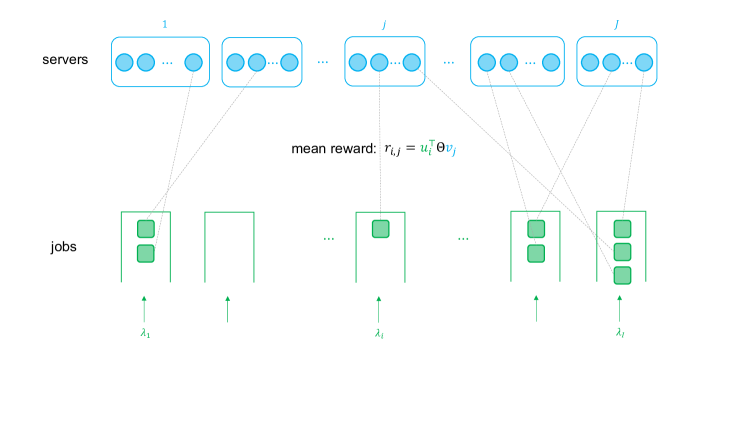
Figure 1: Scheduling system elements: servers of different classes need to be allocated to jobs of different classes. Allocation of a job of class $i$ to a server of class $j$ yields a stochastic reward with mean value according to the bilinear model $r_{i,j}=u_{i}^{\top}\Theta v_{j}$ where $u_{i}$ and $v_{j}$ are feature vectors of job and server classes.

We discuss some properties of the expected allocation defined as the solution of (4). By the Karush-Kuhn-Tucker (KKT) conditions, the solution of (4) is such that, for every $i\in\mathcal{I}$ and $j\in\mathcal{J}$, either

$$y_{i,j}(t)>0 \frac{1}{V}Q_{i}(t)w_{i}\frac{1}{\sum_{j^{\prime}\in\mathcal{J}}y_{i,j^{\prime}}(t)}=\nu_{j}(t)+(\gamma-\hat{r}_{i,j}(t)),\hbox{ or }$$ and (5)

$$y_{i,j}(t)=0 \frac{1}{V}Q_{i}(t)w_{i}\frac{1}{\sum_{j^{\prime}\in\mathcal{J}}y_{i,j^{\prime}}(t)}\leq\nu_{j}(t)+(\gamma-\hat{r}_{i,j}(t))$$ and (6)

where $\nu_{j}(t)\geq 0$ are Lagrange multipliers associated with server capacity constraints, satisfying $\nu_{j}(t)(n_{j}-\sum_{i^{\prime}\in\mathcal{I}(t)}y_{i^{\prime},j}(t))=0$. Intuitively, (5)-(6) is a condition that requires balancing marginal utility of a job class with marginal cost for any server class for which this job class has a positive allocation. Indeed, the marginal utility in the left-hand side in equation (5) is decreasing in $\sum_{j^{\prime}\in\mathcal{J}}y_{i,j^{\prime}}(t)$ and the marginal cost in the right-hand side of equation (5) is decreasing in $\hat{r}_{i,j}(t)$. Hence, for fixed value of $\nu_{j}(t)$, the larger the $\hat{r}_{i,j}(t)$, the larger the allocation $\sum_{j^{\prime}\in\mathcal{J}}y_{i,j^{\prime}}(t)$. From the conditions in (5)-(6), it can be observed that each job class has a strictly positive expected allocation by some server class.

We evaluate the performance of a scheduling algorithm with respect to the expected total reward of assignments over initial $T$ time steps, and mean queue lengths of job classes at any time. For the reward objective, we consider regret defined as the difference of the cumulative reward of an oracle policy and the cumulative reward of the algorithm over the time horizon. The oracle policy is based on the assumption that mean rewards $r_{i,j}$ and traffic intensity parameters $\rho_{i}$ are known. Let $p^{*}=(p^{*}_{i,j},i\in\mathcal{I},j\in\mathcal{J})$ be the solution of the following optimization problem, which specifies fractional allocation of jobs to servers according to the oracle policy:

$$\begin{array}[]{rl}\mbox{maximize}&\sum_{i\in\mathcal{I}}\sum_{j\in\mathcal{J}}r_{i,j}\rho_{i}p_{i,j}\\ \mbox{subject to}&\sum_{i\in\mathcal{I}}\rho_{i}p_{i,j}\leq n_{j}\mbox{ for all }j\in\mathcal{J}\\ &\sum_{j\in\mathcal{J}}p_{i,j}=1\mbox{ for all }i\in\mathcal{I}\\ \mbox{over}&p_{i,j}\geq 0,\hbox{ for all }i\in\mathcal{I},j\in\mathcal{J}.\end{array}$$

Let $\mathcal{I}(t)$ be the set of job classes that wait to be served at time $t$, i.e. $\mathcal{I}(t)=\{i\in\mathcal{I}:Q_{i}(t)>0\}$. Then the regret of an algorithm with expected random allocation $(y_{i,j}(t),i\in\mathcal{I}(t),j\in\mathcal{J},t\in\{1,\ldots,T\})$ is defined as

$$R(T)=T\sum_{i\in\mathcal{I}}\sum_{j\in\mathcal{J}}r_{i,j}\rho_{i}p_{i,j}^{*}-\sum_{t=1}^{T}\sum_{i\in\mathcal{I}(t)}\sum_{j\in\mathcal{J}}r_{i,j}y_{i,j}(t).$$

Additional notation.

For any $d\in\mathbb{Z}_{+}$, the weighted norm of vector $x\in\mathbb{R}^{d}$ with the weight matrix $A\in\mathbb{R}^{d\times d}$ is defined as $\|x\|_{A}=\sqrt{x^{\top}Ax}$. We use $\tilde{O}(\cdot)$ to hide poly-logarithmic factors.

3 Algorithm and performance guarantees

In this section, we present our main results including an algorithm and its performance guarantees with respect to regret and mean queue lengths for a scheduling algorithm based on weighted proportionally fair allocation criteria with assignment costs, which we present in Section 3.1. These results are established under assumption that mean service times are identical for jobs of different classes and that the set of servers is fixed. We present extensions of our results in Section 3.3 that allow for mean service times to be different across job classes and for the set of servers to be time varying.

3.1 Algorithm

We consider an algorithm that uses recursive estimation of mean rewards which are used for determining the expected allocation of jobs to servers in each time step according to the solution of the optimization problem (4). In each time step, having computed the expected allocation of jobs to servers, the assignments are realized by a randomized allocation procedure. The algorithm is defined in Algorithm 1.

The algorithm uses a randomized allocation for assigning servers to jobs which assigns $y_{i,j}(t)$ servers of class $j$ to jobs of class $i$ in expectation. This is realized such that each server of class $j\in\mathcal{J}$ selects a job $k\in\mathcal{Q}(t)$ with probability $y_{\upsilon(k),j}(t)/(n_{j}Q_{\upsilon(k)}(t))$, where recall $\upsilon(k)$ denotes the class of job $k$. This is a non work-conserving scheduling policy if $\sum_{i\in\mathcal{I}(t)}y_{i,j}(t)<n_{j}$ for some server class $j\in\mathcal{J}$ and some time step $t\geq 1$, because a server of class $j\in\mathcal{J}$ is not assigned a job in time step $t$ with probability $1-\sum_{k\in\mathcal{Q}(t)}y_{\upsilon(k),j}(t)/(n_{j}Q_{\upsilon(k)}(t))$. At each time step, each server class can make at most $n_{j}$ job selections, respecting its capacity constraint. When it selects a job $k^{*}\in\mathcal{Q}(t)$, then the algorithm can assign this job and observe the value of stochastic reward. Note that a service unit of a job may be assigned to more than one server, which is beneficial for estimation of mean rewards.

Algorithm 1 Scheduling Algorithm for Bilinear Rewards (SABR)

Initialize: $\Lambda^{-1}\leftarrow(1/\zeta)I_{d^{2}\times d^{2}}$, $b\leftarrow 0_{d^{2}\times 1}$

for $t=1,\ldots,T$ do

    Update parameter estimator $\hat{\theta}\leftarrow\Lambda^{-1}b$

    Update mean reward estimators $\tilde{r}_{i,j}\leftarrow w_{i,j}^{\top}\hat{\theta}+\sqrt{w_{i,j}^{\top}\Lambda^{-1}w_{i,j}\beta(t)}$, for $i\in\mathcal{I}(t)$ and $j\in\mathcal{J}$

    Set expected allocation $(y_{i,j},i\in\mathcal{I}(t),j\in\mathcal{J})$ to the solution of (4) with $(\hat{r}_{i,j}(t)=\Pi_{[-1,1]}(\tilde{r}_{i,j}),i\in\mathcal{I}(t),j\in\mathcal{J})$

    $(\xi_{l,j},\upsilon_{l,j},j\in[J],l\in[n_{j}])\leftarrow$ Randomized_allocation($(y_{i,j},i\in\mathcal{I}(t),j\in\mathcal{J}),(\mathcal{Q}_{i}(t),i\in\mathcal{I}(t))$)

    for $j=1,\ldots,J$ do

       for $l=1,\ldots,n_{j}$ do

          $i\leftarrow\upsilon_{l,j}$

          if $i\neq 0$ then

             $\Lambda^{-1}\leftarrow\Lambda^{-1}-\frac{\Lambda^{-1}w_{i,j}w_{i,j}^{\top}\Lambda^{-1}}{1+w_{i,j}^{\top}\Lambda^{-1}w_{i,j}}$

             $b\leftarrow b+w_{i,j}\xi_{l,j}$

          end if

       end for

    end for

end for

// randomized allocation procedure

function Randomized_allocation($(y_{i,j},i\in\mathcal{I}(t),j\in\mathcal{J}),(\mathcal{Q}_{i}(t);i\in\mathcal{I}(t))$)

    for $j=1,\ldots,J$ do

       for $l=1,\ldots,n_{j}$ do

          Choose a job $k^{*}\in\mathcal{Q}(t)$ randomly according to probabilities $y_{\upsilon(k),j}/(n_{j}Q_{\upsilon(k)}(t))$ for all $k\in\mathcal{Q}(t)$,

          or, choose no job with probability $1-\sum_{k\in\mathcal{Q}(t)}y_{\upsilon(k),j}/(n_{j}Q_{\upsilon(k)}(t))$

          $\upsilon_{l,j}\leftarrow 0$

          if job $k^{*}$ is chosen then

             Assign server $l$ of class $j$ to job $k^{*}$ to process one service unit of this job

             $\upsilon_{l,j}\leftarrow\upsilon(k^{*})$

          end if

       end for

    end for

    Observe rewards of assigned jobs $(\xi_{l,j},l=1,\ldots,n_{j},j=1,\ldots,J\hbox{ such that }\upsilon_{l,j}\neq 0)$

    return $\xi_{l,j}$, $\upsilon_{l,j}$ for $l\in[n_{j}]$, $j\in[J]$

end function

A key component of the algorithm are recursive mean reward estimators, which are designed for the underlying bilinear model. These estimators require estimating the unknown parameter $\theta$ from partial feedback and accounting for the trade-off between exploration and exploitation. The algorithm adopts the strategy of optimism in the face of uncertainty for linear bandits (Abbasi-Yadkori et al. 2011) for computing upper confidence bound (UCB) indices for mean rewards of job-server assignments. Let $\upsilon_{l,j}(t)$ be the class of job selected in the $l$-th selection by server class $j$ and let $\xi_{l,j}(t)$ be the observed reward of this selection. The feature vector of a combination of job class $i$ and server class $j$ is defined as $w_{i,j}=\mathrm{vec}(u_{i}v_{j}^{\top})$. For simplicity of notation, we write $w_{l,j}(t)=w_{\upsilon_{l,j}(t),j}$. At each time step $t$, the algorithm uses an estimator of $\theta$ defined as

$$\hat{\theta}(t)=\Lambda(t)^{-1}b(t)$$

where, for a parameter $\zeta>0$,

$$\Lambda(t)=\zeta I_{d^{2}\times d^{2}}+\sum_{s=1}^{t-1}\sum_{j\in\mathcal{J}}\sum_{l\in[n_{j}]}w_{l,j}(s)w_{l,j}(s)^{\top}$$

and

$$b(t)=\sum_{s=1}^{t-1}\sum_{j\in\mathcal{J}}\sum_{l=1}^{n_{j}}w_{l,j}(s)\xi_{l,j}(s).$$

The mean reward estimator $\hat{r}_{i,j}(t)$ is defined to be the maximum reward over a confidence set ${\mathcal{C}}(t)$ constrained to take values in $[-a,a]$. Specifically, we let

$$\tilde{r}_{i,j}(t):=\max\{w_{i,j}^{\top}\theta^{\prime}:\theta^{\prime}\in{\mathcal{C}}(t)\}$$

where ${\mathcal{C}}(t)$ is the confidence set defined as

$${\mathcal{C}}(t)=\left\{\theta^{\prime}\in\mathbb{R}^{d^{2}}:\|\hat{\theta}(t)-\theta^{\prime}\|_{\Lambda(t)}\leq\sqrt{\beta(t)}\right\}$$

with $\sqrt{\beta(t)}:=\kappa\sqrt{d^{2}\log(tT)}+\sqrt{\zeta}$.

Then, we set $\hat{r}_{i,j}(t)=\Pi_{[-a,a]}(\tilde{r}_{i,j}(t))$, where $\Pi_{[a_{1},a_{2}]}(x):=\max\{a_{1},\min\{x,a_{2}\}\}$. This truncation step is used because the mean rewards always lie in $[-a,a]$, and is important for the regret guarantees that mean reward estimates lie in a bounded set, which will be evident later when we discuss regret guarantees. The mean reward estimates $\hat{r}_{i,j}(t)$ can be computed by using iterative updates, which is discussed as follows. Note that $\tilde{r}_{i,j}(t)=w_{i,j}^{\top}(\hat{\theta}(t)+\Delta^{*}_{i,j}(t))$ where $\Delta^{*}_{i,j}(t)$ is a maximizer of the following convex optimization problem with a linear objective function and a quadratic constraint:

$$\begin{array}[]{rl}\mbox{maximize}&w_{i,j}^{\top}\Delta\\ \mbox{subject to}&\Delta^{\top}\Lambda(t)\Delta\leq\beta(t)\\ \mbox{over}&\Delta\in\mathbb{R}^{d^{2}}.\end{array}$$ (10)

It can be readily shown that the optimization problem (10) has a unique maximizer given by

$$\Delta^{*}_{i,j}(t)=\frac{\sqrt{\beta(t)}}{\sqrt{w_{i,j}^{\top}\Lambda(t)^{-1}w_{i,j}}}\Lambda(t)^{-1}w_{i,j}.$$ (11)

It follows that

$$\tilde{r}_{i,j}(t)=w_{i,j}^{\top}\hat{\theta}(t)+\sqrt{w_{i,j}^{\top}\Lambda(t)^{-1}w_{i,j}}\sqrt{\beta(t)}.$$

The algorithm iteratively computes the inverse matrix $\Lambda(t)^{-1}$ by using the Sherman-Morrison formula (Hager 1989) by exploiting the fact that $\Lambda(t)$ is defined as a weighted sum of an identity matrix and rank 1 matrices. This amounts to a $O((nd^{4}+IJd^{4})T)$ total computation cost for computing the mean reward estimators, where the first term is due to the computation of the inverse matrix $\Lambda(t)^{-1}$ and the second term is due to the computation of the mean reward estimators over the time horizon. Note that in Algorithm 1 at each time step $t$, we may update $\tilde{r}_{i,j}$ only for job classes for which there is at least one job of this class waiting to be served, which would yield some computation efficiency gains.

3.2 Regret and queue length analysis

In this section we provide regret and queue length analysis for the case of identical mean job service times. We consider extensions allowing for non-identical mean job service times and allowing also for time-varying set of server classes later in Section 3.3.

For the queuing system stability, we assume that $\rho/n<1$. The system’s stability region is defined as the set of job arrival rate vectors $(\lambda_{1},\ldots,\lambda_{I})$ for which the condition $\rho/n<1$ holds (Tassiulas and Ephremides 1992, Mandelbaum and Stolyar 2004). For the case of identical mean job service times, this condition corresponds to $\lambda<\mu n$.

We assume that $1/T\leq\mu\leq 1$ and $T\geq n$. In other words, the time horizon is assumed to be larger or equal to the mean job service time and the number of servers, and the mean job service time is assumed to be larger than or equal to one time step.

Let $w_{\min}=\min_{i\in\mathcal{I}}w_{i}$, $w_{\max}=\max_{i\in\mathcal{I}}w_{i}$, $\rho_{\min}=\min_{i\in\mathcal{I}}\rho_{i}$, and $\tilde{\rho}_{\min}=\min_{i\in\mathcal{I}}\rho_{i}/w_{i}$. To simplify notation, we define $c_{a,\gamma}=(\gamma+a)/(\gamma-a)$ for $0<a<\gamma$, which corresponds to the ratio of the maximum and minimum marginal cost. We show a regret bound of Algorithm 1 in the following theorem.

Theorem 3.1

The regret of Algorithm 1 with $\zeta=an$ and any $V>0$ and $\gamma>a$, satisfies

$$R(T)=\tilde{O}\left(\frac{1}{\mu}\left(\alpha_{1}V\frac{1}{w_{\min}}+\alpha_{2}\frac{w_{\max}}{w_{\min}}\right)+\frac{1}{V}\left(\alpha_{3}\frac{1}{\tilde{\rho}_{\min}}+\sum_{i\in\mathcal{I}}w_{i}\right)T+(\alpha_{4}d^{2}+\alpha_{5}d)\sqrt{T}\right),$$

where $\alpha_{1}=\gamma^{2}n$, $\alpha_{2}=\gamma c_{a,\gamma}n^{2}/(1-\rho/n)$, $\alpha_{3}=c_{a,\gamma}^{2}n^{2}$, $\alpha_{4}=a\sqrt{n}$, and $\alpha_{5}=an$.

Proof 3.2

Proof. The proof is available in Appendix 8.

The regret bound in Theorem 3.1 has three terms. The first term is proportional to the expected queue length at the time horizon. The second term is due to stochasticity in job departures because of using a randomized allocation. The last term comes from the bandit algorithm used for learning mean rewards of assignments. Note that by using the linear bandit algorithm, this term does not depend on either the number of job classes $I$ or the number of server classes $J$, but depends on $d$ (the dimension of feature vectors of jobs and servers). In some practical situations, $d$ can be much smaller than $I$ and $J$.

Note that for any weight parameters $w_{1},\ldots,w_{I}$, the smallest regret bound in Theorem 3.1 is achieved for the case of identical weight parameters such that $w_{i}=w_{\min}$, for all $i\in\mathcal{I}$. This is intuitive as the job weight parameters may negatively affect the rewards accrued by the assignments.

From Theorem 3.1, by optimizing the value of parameter $V$, we have the regret bound

$$\tilde{O}\left(\left(\sqrt{\frac{\alpha_{1}}{\mu w_{\min}}\left(\alpha_{3}\frac{1}{\tilde{\rho}_{\min}}+\sum_{i\in\mathcal{I}}w_{i}\right)}+\alpha_{4}d^{2}+\alpha_{5}d\right)\sqrt{T}+\frac{1}{\mu}\alpha_{2}\frac{w_{\max}}{w_{\min}}\right),$$ (12)

which is obtained for $V=\sqrt{(\alpha_{3}/\tilde{\rho}_{\min}+\sum_{i\in\mathcal{I}}\omega_{i})\mu w_{\min}/\alpha_{1}}$.

For identical job weight parameters, we have the regret bound

$$\tilde{O}\left(\left(\sqrt{\alpha_{1}\alpha_{3}\frac{1}{\mu\rho_{\min}}}+\alpha_{4}d^{2}+\alpha_{5}d\right)\sqrt{T}+\frac{1}{\mu}\alpha_{2}\right).$$ (13)

This optimized regret bound requires information about normalized minimum traffic intensity $\min_{i\in\mathcal{I}}\rho_{i}/w_{i}$ for setting the parameter $V$. We can achieve the following regret bound by setting parameter $V$ without requiring any information about traffic intensities

$$\tilde{O}\left(\left(\sqrt{\frac{\alpha_{1}(\alpha_{3}+\sum_{i\in\mathcal{I}}\frac{w_{i}}{w_{\min}})}{\mu}}\left(1+\frac{\frac{\alpha_{3}}{w_{\min}\tilde{\rho}_{\min}}+\sum_{i\in\mathcal{I}}\frac{w_{i}}{w_{\min}}}{\alpha_{3}+\sum_{i\in\mathcal{I}}\frac{w_{i}}{w_{\min}}}\right)+\alpha_{4}d^{2}+\alpha_{5}d\right)\sqrt{T}+\frac{1}{\mu}\alpha_{2}\frac{w_{\max}}{w_{\min}}\right)$$ (14)

which is achieved for $V=\sqrt{(\alpha_{3}+\sum_{i\in\mathcal{I}}w_{i}/w_{\min})\mu/\alpha_{1}}\sqrt{T}$.

The key difference between the regret bounds in (12) and (14) is that the former scales with $\tilde{\rho}_{\min}$ as $\sqrt{1/\tilde{\rho}_{\min}}$ while the latter scales as $1/\tilde{\rho}_{\min}$. In the case when traffic intensities are within a constant factor from each other, in both cases, the regret scales as $\sqrt{I}$ with the number of job classes.

We compare our regret bound with the regret bound by Hsu et al. (2021). We first remark that $\tilde{O}((\sqrt{n}d^{2}+nd)\sqrt{T})$ in the regret bound in Theorem 3.1, which recall is due to the bandit algorithm, is sublinear in $T$, growing as $\sqrt{T}$. This is in contrast to the corresponding term in the regret bound in Hsu et al. (2021) which is linear in $T$. This improvement is achieved by leveraging the bilinear structure of rewards so that mean rewards are learned by aggregating observed information per each job class, unlike to Hsu et al. (2021) where learning of the mean rewards is conducted independently per each job. Furthermore, under the assumption that $\rho/n$ is constant, it holds $\rho=\Theta(n)$, and the corresponding term in Hsu et al. (2021) is $\tilde{O}(n^{2}JT)$. Our bound has a better scaling with the number of server classes $J$ when $d^{2}$ is much smaller than $J$. This is because our algorithm performs learning per each job class and leverages the bilinear structure of rewards.

We consider the holding cost defined as $\sum_{i\in\mathcal{I}}c_{i}Q_{i}(t)$ at time $t$, where $c_{1},\ldots,c_{I}>0$ are some marginal holding cost parameters. Let $c_{\max}=\max_{i\in\mathcal{I}}c_{i}$. In the following theorem, we provide a bound for the mean holding cost.

Theorem 3.3

Algorithm 1 guaranteees the following bound on the mean holding cost, for any $V>0$, $\gamma>a$, and $t\geq 0$,

$$\sum_{i\in\mathcal{I}}c_{i}\mathbb{E}\left[Q_{i}(t)\right]\leq\frac{1}{\min_{i\in\mathcal{I}}\left\{w_{i}/c_{i}\right\}}\max\left\{(\gamma+a)Vn,2c_{a,\gamma}\frac{n^{2}}{1-\rho/n}w_{\max}\right\}+\frac{1+\rho/n}{1-\rho/n}c_{\max}+c_{\max}.$$

Proof 3.4

Proof. The proof is deferred to Appendix 9.

The bound on the mean holding cost depends on the relative values of the weight parameters $w_{i}$ with respect to the marginal holding cost parameters $c_{i}$. If some job class has a small weight $w_{i}$ relative to the marginal holding cost $c_{i}$, then the bound on the mean holding cost becomes large.

From Theorem 3.3 we have the following bound on the mean queue length, by taking all marginal holding cost parameters to be of value $1$,

$$\mathbb{E}[Q(t)]\leq\max\left\{(\gamma+a)Vn\frac{1}{w_{\min}},2c_{a,\gamma}\frac{n^{2}}{1-\rho/n}\frac{w_{\max}}{w_{\min}}\right\}+\frac{1+\rho/n}{1-\rho/n}+1.$$ (15)

We observe that mean queue length in each time step is bounded by a linear function in $V$, which is common in the framework of queueing system control by using the Lyapunov drift plus penalty method. The larger the value of $V$, the less weight is put on the fairness term in the objective function of the optimization problem in (4). The mean queue length bound has a factor $1/(1-\rho/n)$, which is common for mean queue length bounds. By setting $V$ to the value that optimizes the regret bound in Theorem 3.1, the mean queue length at any time $t\geq 0$ is bounded as

$$\mathbb{E}[Q(t)]=O\left(\sqrt{(\mu/\rho_{\min})T}\right),$$ (16)

by assuming that other parameters are constants.

A special case is when the marginal holding costs are equal to the weights of job classes, i.e. $c_{i}=w_{i}$ for all $i\in\mathcal{I}$. This case has a special meaning because from the KKT conditions (5)-(6), for any $i\in\mathcal{I}$, $j\in\mathcal{J}$, and $t\geq 0$,

$$w_{i}Q_{i}(t)=V\sum_{j\in\mathcal{J}}(\nu_{j}(t)+(\gamma-\hat{r}_{i,j}(t)))y_{i,j}(t).$$

Hence, $w_{i}\mathbb{E}[Q_{i}(t)]/V$ corresponds to the mean cost per unit time that accounts for both shadow prices associated with server capacities and the assignment costs. From Theorem 3.1, we have

$$\sum_{i\in\mathcal{I}}w_{i}\mathbb{E}\left[Q_{i}(t)\right]\leq\max\left\{(\gamma+a)Vn,2c_{a,\gamma}\frac{n^{2}}{1-\rho/n}w_{\max}\right\}+\frac{1+\rho/n}{1-\rho/n}w_{\max}+w_{\max}.$$

Reducing the computation cost.

We remark that the same bound as in Theorem 3.1 holds for a variant of Algorithm 1 that updates the mean reward estimators only at some time steps. Specifically, the mean reward estimators only need to be updated at $O(d^{2}\log(T))$ time steps over a horizon of $T$ time steps. This is achieved by adopting the method of rarely switching (Abbasi-Yadkori et al. 2011), which amounts to a $O(nd^{4}T+IJd^{6}\log(T))$ computation cost for updating the mean reward estimators. This is an improvement with respect to the computation cost of updating mean reward estimators in Algorithm 1, which is $O((nd^{4}+IJd^{4})T)$, when $T$ is large relative to $d^{2}$. Details are shown in Algorithm 2 and discussion in Appendix 10.

3.3 Extensions

3.3.1 Allowing for non-identical mean job service times

In Sections 3.2, we provided regret analysis under assumption that mean job service times are identical for all jobs. In this section we show that this can be relaxed to allow for non-identical mean job service times over different job classes, under a stability condition. We consider the case when service times of class $i$ jobs follow a geometric distribution with mean $1/\mu_{i}$. Let $\mu_{\min}=\min_{i\in\mathcal{I}}\mu_{i}$ and $\mu_{\max}=\max_{i\in\mathcal{I}}\mu_{i}$. We assume that $2\lambda/\mu_{\min}-\rho<n$ for stability condition, $1/\mu_{\min}\leq T$, and $\mu_{\max}\leq 1$. This stability condition is based on the fact that the job arrival rate is $\lambda$ and the departure rate, which depends on the algorithm, is at least $\mu_{\min}(n+\rho)/2$ in the worst case. Note that for $2\lambda/\mu_{\min}-\rho<n$ to hold, it is sufficient that $\rho/n<1/(2\mu_{\max}/\mu_{\min}-1)$.

We provide a regret and a mean holding cost bound for Algorithm 1 in the following two theorems. We note that from the mean holding cost we can easily obtain a mean queue length bound.

Theorem 3.5

Algorithm 1 with $\zeta=an$ has the regret bound, for any $V>0$ and $\gamma>a$,

$$R(T) =\tilde{O}\left(\frac{1}{\mu_{\min}}\left(\alpha_{1}V\frac{1}{w_{\min}}+\alpha_{2}\frac{w_{\max}}{w_{\min}}\right)+\frac{1}{V}\left(\alpha_{3}\left(\max_{i\in\mathcal{I}}\frac{w_{i}}{\rho_{i}}\right)+\sum_{i\in\mathcal{I}}w_{i}\right)T+(\alpha_{4}d^{2}+\alpha_{5}d)\sqrt{T}\right),$$ (17)

where $\alpha_{1}=\gamma^{2}n$, $\alpha_{2}=\gamma c_{a,\gamma}n^{2}/(1-(2\lambda/\mu_{\min}-\rho)/n)$, $\alpha_{3}=c_{a,\gamma}^{2}n^{2}$, $\alpha_{4}=a\sqrt{n}$, and $\alpha_{5}=an$.

Proof 3.6

Proof. The proof is deferred to Appendix 11.

Theorem 3.7

Algorithm 1 has the mean holding cost bounded as, for any $V>0$, $\gamma>a$, and $t\geq 0$,

$$\sum_{i\in\mathcal{I}}c_{i}\mathbb{E}[Q_{i}(t)]\leq \frac{1}{\min_{i\in\mathcal{I}}\{w_{i}/c_{i}\}}\max\left\{(\gamma+a)Vn_{\max},c_{a,\gamma}\frac{2n_{\max}^{2}}{1-\rho/n_{\min}}w_{\max}\right\}$$

$$\quad+\frac{1+\rho/n_{\min}}{1-(2\lambda/\mu_{\min}-\rho)/n_{\min}}c_{\max}+c_{\max}.$$

Proof 3.8

Proof. This theorem is proven as an intermediate result in the proof of Theorem 3.5.

The regret bound in Theorem 3.5 conforms to the regret bound in Theorem 3.1 that holds for identical mean job service times, with the mean job service time replaced with the maximum mean job service time. The dependence of the regret bound on the parameters $n$, $I$, $J$ and $T$ remain to hold as in Theorem 3.1. For the special case of identical mean job service times, the mean queue length bound in Theorem 3.7 boils down to the bound in Theorem 15.

3.3.2 Allowing for a time-varying set of server classes

In our analysis of regret so far we assumed that the set of server classes $\mathcal{J}$ is fixed at all times. In this section, we show that this can be relaxed to allow for a time-varying set of server classes under a stability condition. Let $\mathcal{J}(t)$ denote the set of server classes at time $t$. Let $n(t)=\sum_{j\in\mathcal{J}(t)}n_{j}$ for each time $t\in\mathcal{T}$. We also define $n_{\min}=\min_{t\in\mathcal{T}}n(t)$, and $n_{\max}=\max_{t\in\mathcal{T}}n(t).$ Assume that $2(\lambda/\mu_{\min})-\rho<n_{\min}$ for a stability condition and $n_{\max}\leq T$. This stability condition is based on the fact that the job arrival rate is $\lambda$ and the departure rate, which depends on the algorithm, is at least $(n_{\min}+\rho)\mu_{\min}/2$. In particular, if mean job service times are identical over job classes, then the stability condition boils down to $\rho<n_{\min}$.

We provide a regret and a mean holding cost bound for Algorithm 1 in the following two theorems. We note that from the mean holding cost we can easily obtain a mean queue length bound.

Theorem 3.9

Algorithm 1 with $\zeta=an_{\max}$ has the regret bound, for any $V>0$ and $\gamma>a$,

$$R(T) =\tilde{O}\left(\frac{1}{\mu_{\min}}\left(\alpha_{1}V\frac{1}{w_{\min}}+\alpha_{2}\frac{w_{\max}}{w_{\min}}\right)+\frac{1}{V}\left(\alpha_{3}\left(\max_{i\in\mathcal{I}}\frac{w_{i}}{\rho_{i}}\right)+\sum_{i\in\mathcal{I}}w_{i}\right)T+(\alpha_{4}d^{2}+\alpha_{5}d)\sqrt{T}\right),$$

where $\alpha_{1}=\gamma^{2}n_{\max}$, $\alpha_{2}=\gamma c_{a,\gamma}n_{\max}^{2}/(1-(2\lambda/\mu_{\min}-\rho)/n_{\min})$, $\alpha_{3}=c_{a,\gamma}^{2}n_{\max}^{2}$, $\alpha_{4}=a\sqrt{n_{\max}}$, and $\alpha_{5}=an_{\max}$.

Proof 3.10

Proof. The proof is deferred to Appendix 12.

Theorem 3.11

Algorithm 1 has the mean queue length bounded as, for any $V>0$ and $\gamma>a$, and $t\geq 0$,

$$\sum_{i\in\mathcal{I}}c_{i}\mathbb{E}[Q_{i}(t)] \leq\frac{1}{\min_{i\in\mathcal{I}}\{w_{i}/c_{i}\}}\max\left\{(\gamma+a)Vn_{\max},c_{a,\gamma}\frac{2n_{\max}^{2}}{1-\rho/n_{\min}}w_{\max}\right\}$$

$$\quad+\frac{1+\rho/n_{\min}}{1-(2\lambda/\mu_{\min}-\rho)/n_{\min}}c_{\max}+c_{\max}.$$

Proof 3.12

Proof. The proof is provided as an intermediate result in the proof of Theorem 3.9.

For the special case when the set of server classes is fixed at all times, the regret bound in Theorem 3.9 and the mean queue length bound in Theorem 3.11 conform to the bounds in Theorem 3.5 and Theorem 3.7, respectively.

4 Distributed allocation algorithms

The scheduling algorithm defined in Algorithm 1 can be run by a dedicated compute node in a centralized implementation. For large-scale systems with many jobs and servers, it is of interest to consider distributed scheduling algorithms, where computations are performed by nodes representing jobs or servers. The part of the algorithm concerned with the computation of mean reward estimators can be easily distributed. The part concerned with the computation of expected allocations of jobs to servers requires solving the convex optimization problem (4) in each time step. We next discuss distributed iterative algorithms for computing these allocations where iterative updates are performed by either nodes representing jobs or servers. These iterative updates are performed according to projected gradient-descent algorithms with feedback delays due to distributed computation. We provide stability conditions for convergence of these iterative algorithms.

In what follows, we consider an arbitrary time step $t$ and omit reference to $t$ in our notation, and write $\mathcal{Q}$ in lieu of $\mathcal{Q}(t)$ and $\mathcal{I}_{+}$ in lieu of $\mathcal{I}(t)$. With a slight abuse of notation, we let $y_{i,j}(r)$ denote the value of allocation for a job-server class combination $(i,j)$ at iteration $r$, for $i\in\mathcal{I}_{+}$ and $j\in\mathcal{J}$, and let $y(r)=(y_{i,j}(r),i\in\mathcal{I}_{+},j\in\mathcal{J})$. We consider iterative updates of allocations under assumption that the set of jobs and mean reward estimators are fixed. This is a standard assumption when studying such iterative allocation updates in network resource allocation problems. In practical applications, such iterative updates would be run at a faster timescale than the timescale at which the set of jobs and mean reward estimates change. We refer to the node maintaining state for a job class $i\in\mathcal{I}$ as job-node $i$, and the node maintaining state for a server class $j\in\mathcal{J}$ as server-node $j$. Let $\tau_{i,j}$ be the delay for communicating information from job-node $i$ to server-node $j$, and let $\tau_{j,i}$ be the delay for communicating information in the other direction, from server-node $j$ to job-node $i$. Let $\tau_{(i,j)}$ be the round-trip delay for job-server class combination $(i,j)$, defined as $\tau_{(i,j)}=\tau_{i,j}+\tau_{j,i}$.

Allocation computed by job nodes.

We first consider distributed computation where each job-node $i\in\mathcal{I}_{+}$ computes $(y_{i,j}(r),j\in\mathcal{J},r\geq 0)$ by using the following iterative updates:

$$y_{i,j}(r+1)=y_{i,j}(r)+\alpha_{i,j}\left(1-\frac{\lambda_{i,j}(r)}{u^{\prime}_{i}(y^{\dagger}_{i}(r))}\right)_{y_{i,j}(r)}^{+}$$ (18)

where $\lambda_{i,j}(r)=p_{j}\left(y^{\S}_{j}(r-\tau_{j,i})\right)+\gamma-\hat{r}_{i,j}$, $y^{\dagger}_{i}(r)=\sum_{j\in\mathcal{J}}y_{i,j}(r-\tau_{(i,j)})$, $y^{\S}_{j}(r)=\sum_{i^{\prime}\in\mathcal{I}_{+}}y_{i^{\prime},j}(r-\tau_{i^{\prime},j})$, $\alpha_{i,j}>0$ is a step size parameter, $u_{i}(y)=(1/V)|\mathcal{Q}|\log(y)$, $p_{j}$ is a non-negative continuously differentiable function with strictly positive derivative, and $(b)_{a}^{+}=b$ if $a>0$ and $(b)_{a}^{+}=\max\{b,0\}$ if $a=0$. Note that $y_{i}(r)$ can be interpreted as allocation to job-node $i$ acknowledged via feedback from server-nodes $j\in\mathcal{J}$.

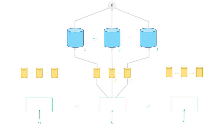
Figure 2: Distributed allocation computation corresponds to a multi-path flow control with a job class node as a source and a virtual receiver node. A path $(i,j)$ originates at job node $i$, traverses a link used exclusively by this path with a marginal price $\gamma-\hat{r}_{i,j}$ and then traverses link $j$ corresponding to a job server node, and finally terminates at the receiver node.

We study convergence properties of the above iterative method in continuous time by considering the corresponding system of delay differential equations:

$$\frac{d}{dr}y_{i,j}(r)=\alpha_{i,j}\left(1-\frac{\lambda_{i,j}(r)}{u_{i}^{\prime}(y^{\dagger}_{i}(r))}\right)_{y_{i,j}(r)}^{+},i\in\mathcal{I}_{+},j\in\mathcal{J}.$$ (19)

Let $C_{j}(z)=\int_{0}^{z}p_{j}(u)du$ for $j\in\mathcal{J}$. An allocation $y=(y_{i,j},i\in\mathcal{I}_{+},j\in\mathcal{J})$ is said to be an equilibrium point of (19) if it is a solution of the following convex optimization problem

$$\begin{array}[]{rl}\mathrm{maximize}&\sum_{i\in\mathcal{I}_{+}}u_{i}(y^{\dagger}_{i})-\sum_{j\in\mathcal{J}}(C_{j}(y^{\S}_{j})+\sum_{i\in\mathcal{I}_{+}}(\gamma-\hat{r}_{i,j})y_{i,j})\\ \mbox{subject to}&y^{\dagger}_{i}=\sum_{j\in\mathcal{J}}y_{i,j},i\in\mathcal{I}_{+}\\ &y^{\S}_{j}=\sum_{i\in\mathcal{I}_{+}}y_{i,j},j\in\mathcal{J}\\ \mathrm{over}&y_{i,j}\geq 0,i\in\mathcal{I}_{+},j\in\mathcal{J}.\end{array}$$ (20)

The objective function of (20) is maximized at $y$ if, and only if, for all $i\in\mathcal{I}_{+}$ and $j\in\mathcal{J}$,

$$y_{i,j}\geq 0,$$ (21)

$$u_{i}^{\prime}(y^{\dagger}_{i})-p_{j}(y^{\S}_{j})-(\gamma-\hat{r}_{i,j})\geq 0,\hbox{ and }$$ (22)

$$y_{i,j}\left(u_{i}^{\prime}(y^{\dagger}_{i})-p_{j}(y^{\S}_{j})-(\gamma-\hat{r}_{i,j})\right)=0.$$ (23)

A point $y$ satisfying (21)-(23) is said to be an interior point if either (21) or (22) holds with strict inequalities. Note that optimization problem (20) is identical to optimization problem (4) except for replacing the hard capacity constraint associated with each server class $j\in\mathcal{J}$ with a soft penalty function $C_{j}$ in the objective function. The iterative updates (18) are of gradient descent type as, when all feedback communication delays are equal to zero, we have $1-\lambda_{i,j}(r)/u_{i}^{\prime}(y^{\dagger}_{i}(r))=(1/u_{i}^{\prime}(y^{\dagger}_{i}(r)))\partial f(y(r))/\partial y_{i,j}(r)$ where $f$ is the objective function of the optimization problem (20).

The system of delay differential equations (19) and the optimization problem (20) correspond to special instance of a joint routing and rate control problem formulation studied in Kelly and Voice (2005) where $(i,j)$ is the index of a route, $i$ is the index of a source, $j$ is the index of a link, and each route $(i,j)$ passes through link $j$ with cost function $C_{j}$ and a link with a fixed price per unit flow $\gamma-\hat{r}_{i,j}\geq 0$ that is used by route $(i,j)$ exclusively. See Figure 2 for an illustration.

Allocation computed by server nodes.

Another distributed algorithm for computing a maximizer $y$ of the optimization problem (20) is defined by letting each server-node $j\in\mathcal{J}$ compute values $(y_{i,j}(r),i\in\mathcal{I}_{+},r\geq 0)$ by using iterative updates with the associated system of delay differential equations:

$$\frac{d}{dr}y_{i,j}(r)=\alpha_{i,j}\left(1-\frac{\lambda_{i,j}(r)}{u^{\prime}_{i}(y^{\dagger}_{i}(r-\tau_{i,j}))}\right)_{y_{i,j}(r)}^{+},i\in\mathcal{I}_{+},j\in\mathcal{J}$$ (24)

where $\lambda_{i,j}(r)=p_{j}\left(\tilde{y}_{j}(r)\right)+\gamma-\hat{r}_{i,j}$, $y^{\dagger}_{i}(r)=\sum_{j^{\prime}\in\mathcal{J}}y_{i,j^{\prime}}(r-\tau_{j^{\prime},i}),$ and $y^{\S}_{j}(r)=\sum_{i^{\prime}\in\mathcal{I}_{+}}y_{i^{\prime},j}(r-\tau_{(i^{\prime},j)}).$ Note that $y^{\S}_{j}(r)$ can be interpreted as the total allocation given by server class $j$ acknowledged to be received by job-nodes $i\in\mathcal{I}_{+}$ via feedback sent to server-node $j$.

Stability condition.

We provide a condition that ensures convergence of $(y^{\dagger}(r),y^{\S}(r))$ as $r$ goes to infinity to a unique point that corresponds to the solution of optimization problem (20), where $(y^{\dagger}(r),y^{\S}(r))$ evolves according to either the system of delay differential equations (19) or (24). We define $\tau_{\max}$ to be an upper bound on the round-trip delay for each job-server class combination, i.e. $\tau_{(i,j)}\leq\tau_{\max}$, for all $i\in\mathcal{I}_{+}$, $j\in\mathcal{J}$.

Theorem 4.1

Assume that $y^{*}$ is an interior equilibrium point, ${y^{*}}^{\dagger}:=(\sum_{i\in\mathcal{J}}y_{i,j}^{*},i\in\mathcal{I}_{+})$, ${y^{*}}^{\S}:=(\sum_{i\in\mathcal{I}_{+}}y_{i,j}^{*},j\in\mathcal{J})$, and that the following condition holds

$$\alpha_{i,j}\tau_{(i,j)}\left(1+\frac{p_{j}^{\prime}({y_{j}^{*}}^{\S}){y_{j}^{*}}^{\S}}{p_{j}({y_{j}^{*}}^{\S})+\gamma-\hat{r}_{i,j}}\right)<\frac{\pi}{2},\hbox{ for all }i\in\mathcal{I}_{+},j\in\mathcal{J}.$$ (25)

Then, there exists a neighborhood $\mathcal{N}$ of $y^{*}$ such that for any initial trajectory $\{y(r),-\tau_{\max}\leq r\leq 0\}$ lying within $\mathcal{N}$, $(y_{i}^{\dagger}(r),i\in\mathcal{I}_{+})$ and $(y_{j}^{\S}(r),j\in\mathcal{J})$, evolving according to (19) (resp. according to (24)), converge exponentially fast, as $r$ goes to infinity, to the unique points ${y^{*}}^{\dagger}$ and ${y^{*}}^{\S}$, respectively.

For the system of delay differential equations (19), the result in Theorem 4.1 follows from Theorem 2 in Kelly and Voice (2005) because it corresponds to a special instance of a joint routing and rate control problem. The proof follows from the generalized Nyquist stability criterion for a linearized system of delay differential equations. For the system of delay differential equations (24), the proof can also be established by following this approach as shown in Appendix 13.

Theorem 4.1 gives us a sufficient condition for exponentially fast convergence of $(y^{\dagger}(r),y^{\S}(r))$ as $r$ goes to infinity. Intuitively, this sufficient condition requires the step size $\alpha_{i,j}$ to be sufficiently small relative to the reciprocal of the round-trip delay $\tau_{(i,j)}$ and a term involving function $p_{j}$ and its derivative, and the marginal price $\gamma-\hat{r}_{i,j}$, for each job-server class pair $(i,j)$. Note that since $\gamma-\hat{r}_{i,j}\geq 0$, we can replace $\gamma-\hat{r}_{i,j}$ in (25) with $0$ and have a stronger sufficient condition. We next discuss some specific functions $p_{j}$ and the sufficient condition derived from Theorem 4.1 for these functions.

First, suppose $p_{j}$ is the power function $p_{j}(z)=(z/n_{j})^{\beta_{j}}$ for $\beta_{j}>0$, for all $j\in\mathcal{J}$. The larger the value of $\beta_{j}$ the closer $p_{j}$ is to a function that has value zero for $0\leq z<n_{j}$, value $1$ for $z=n_{j}$, and has infinite value for $z>n_{j}$. Note that $p_{j}^{\prime}(y_{j}^{\S})y_{j}^{\S}=\beta_{j}p_{j}(y_{j}^{\S})$, for all $j\in\mathcal{J}$. From Theorem 4.1, we have the following sufficient stability condition

$$\alpha_{i,j}\tau_{(i,j)}<\frac{\pi}{2}\frac{1}{1+\beta_{j}},\hbox{ for all }i\in\mathcal{I}_{+},j\in\mathcal{J}.$$

In this case, the sufficient condition is that the step size $\alpha_{i,j}$ is smaller than a constant factor of $1/\tau_{(i,j)}$, with the constant factor decreasing with $\beta_{j}$.

Second, we can accommodate a broader set of functions than in the previous case as follows. Suppose that $p_{j}$ is such that $p_{j}^{\prime}(z)z\leq\beta_{j}p_{j}(z)$ and $p_{j}(z)\leq\gamma_{j}$ for all $z\geq 0$, for some $\beta_{j}>0$ and $\gamma_{j}>0$, and $\gamma-\hat{r}_{i,j}\geq c$, for all $i\in\mathcal{I}_{+}$, $j\in\mathcal{J}$, for some $c\geq 0$. Then, we have the following sufficient stability condition

$$\alpha_{i,j}\tau_{(i,j)}<\frac{\pi}{2}\frac{\gamma_{j}+c}{\gamma_{j}+\gamma_{j}\beta_{j}+c},\hbox{ for all }i\in\mathcal{I}_{+},j\in\mathcal{J}.$$

Finally, suppose that $p_{j}$ is the function defined as $p_{j}(z)=(z/n_{j})/(1-z/n_{j})$ for all $j\in\mathcal{J}$. Note that this function has a vertical asymptote at $z=n_{j}$. In this case, we have $p^{\prime}_{j}(y_{j}^{\S})y_{j}^{\S}=p_{j}(y_{j}^{\S})(1+p_{j}(y_{j}^{\S}))$. Assume that $y^{*}$ is such that ${y_{j}^{*}}^{\S}/n_{j}\leq 1-\epsilon$ for all $j\in\mathcal{J}$, for some $\epsilon\in(0,1)$. Then, we have the following sufficient stability condition

$$\alpha_{i,j}\tau_{(i,j)}<\frac{\pi}{4}\epsilon,\hbox{ for all }i\in\mathcal{I}_{+},j\in\mathcal{J}.$$

5 Numerical results

In this section we present results of our numerical experiments. The goal of these experiments is to demonstrate how regret and mean queue lengths of our proposed algorithm depend on various parameters, such as weight parameters of weighted proportionally fair criteria, mean job service time, and the number of job and server classes. We refer to Algorithm 1 as SABR (Scheduling Algorithm for Bilinear Rewards) when the weight parameters of weighted proportionally fair allocation criteria are identical and set to value $1$, and, as W-SABR (Weighted Scheduling Algorithm for Bilinear Rewards) when the weights parameters are set to some other values. The experimental results validate our theoretical results. The code is available in the Github repository: https://github.com/junghunkim7786/Scheduling_BilinearRewards.

We consider randomly generated problem instances, as well as instances generated by using a real-world data trace from a large-scale cluster computing system. The randomly generated problem instances allow us to carefully design experiments and vary certain parameters to evaluate their effect on the regret and the mean queue length of an algorithm, while using the real-world data trace allows us to demonstrate applicability and evaluate performance of our algorithm in a cluster computing application scenario. We ran each experiment for 10 independent repetitions and report mean values along with $95\%$ confidence intervals.

5.1 Randomly generated problem instances

Our basic setting for generating random problem instances is defined as follows. We consider the case of identical traffic intensities, i.e. $\rho_{i}=\rho/I$ for all $i\in\mathcal{I}$, and identical number of servers per server class, i.e. $n_{j}=n/J$ for all $j\in\mathcal{J}$, for the number of servers $n$. Specifically, we assume $\rho=1$ and $n=4$, which amounts to the system load $\rho/n=0.25$ (we obtained similar results for different system loads, e.g. $0.125$ and $0.5$, which we omit for brevity). We set $a=1$ for the range of rewards, the mean job service times to be identical equal to $1/\mu$, and set the dimension $d$ of feature vectors to $2$. The mean rewards follow the bilinear model with feature vectors $\{u_{i},\ i\in\mathcal{I}\}$ and $\{v_{j},\ j\in\mathcal{J}\}$ with values of features set to independent samples from a uniform distribution on $[0,1]$ and then normalized such that $\|u_{i}\|_{2}=1$ for all $i\in\mathcal{I}$ and $\|v_{j}\|_{2}=1$ for all $j\in\mathcal{J}$. The elements of the parameter $\theta$ are set to independent samples from a uniform distribution on $[0,1]$ and then normalized such that $\|\theta\|_{2}=1$. Each stochastic reward has a Gaussian noise with mean zero and variance $0.01$.

We set the value of parameter $\gamma$ to $1.2$. The value of parameter $V$ is set to the value that minimizes the regret bound of (12) for given time horizon $T$.

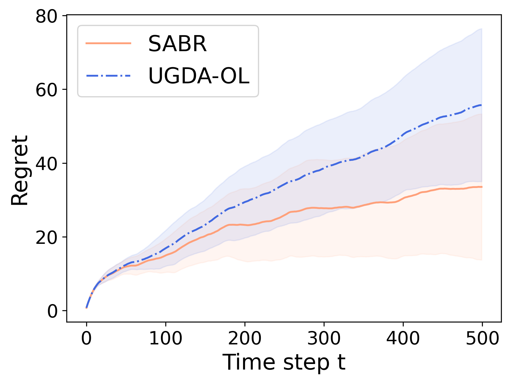
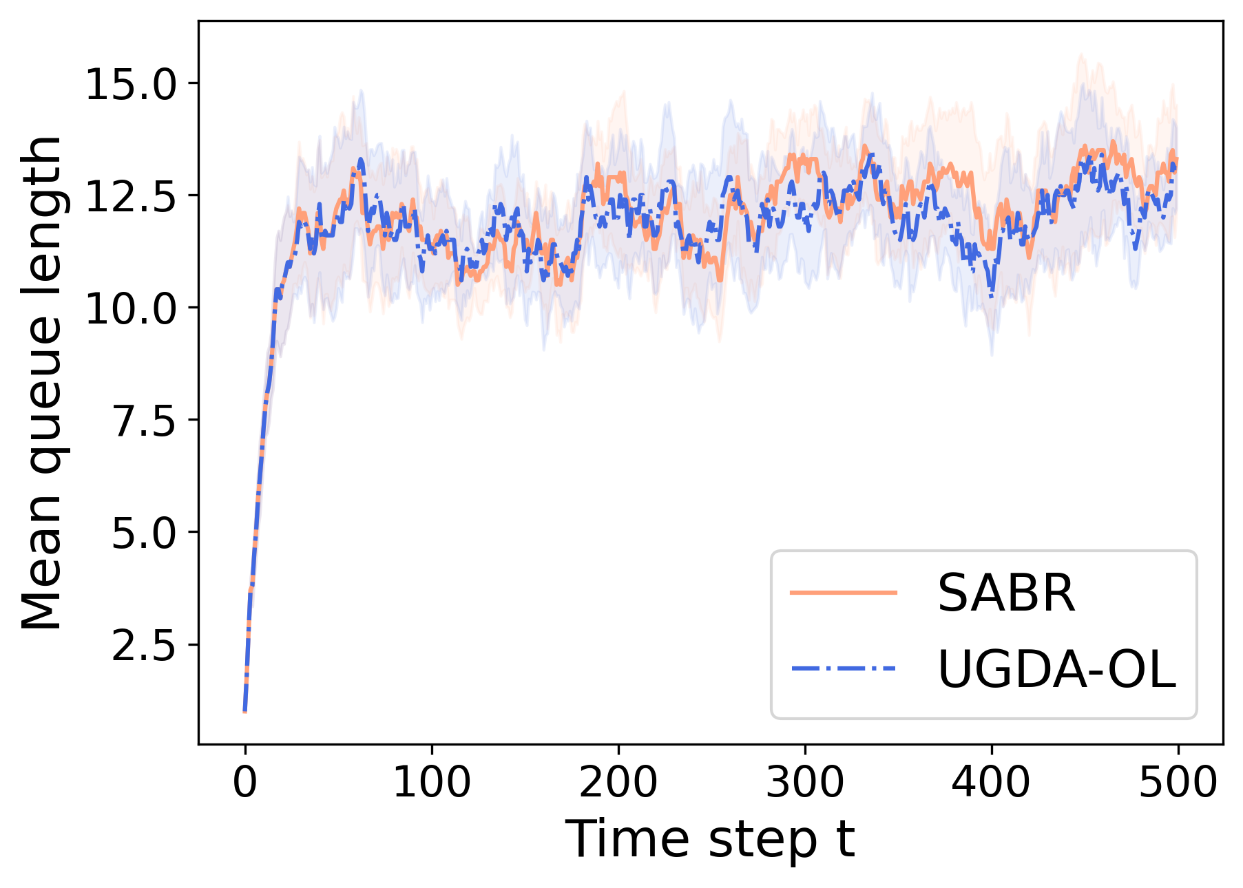
Figure 3: Performance of SABR and UGDA-OL over time steps: (left) reward and (right) mean queue length.

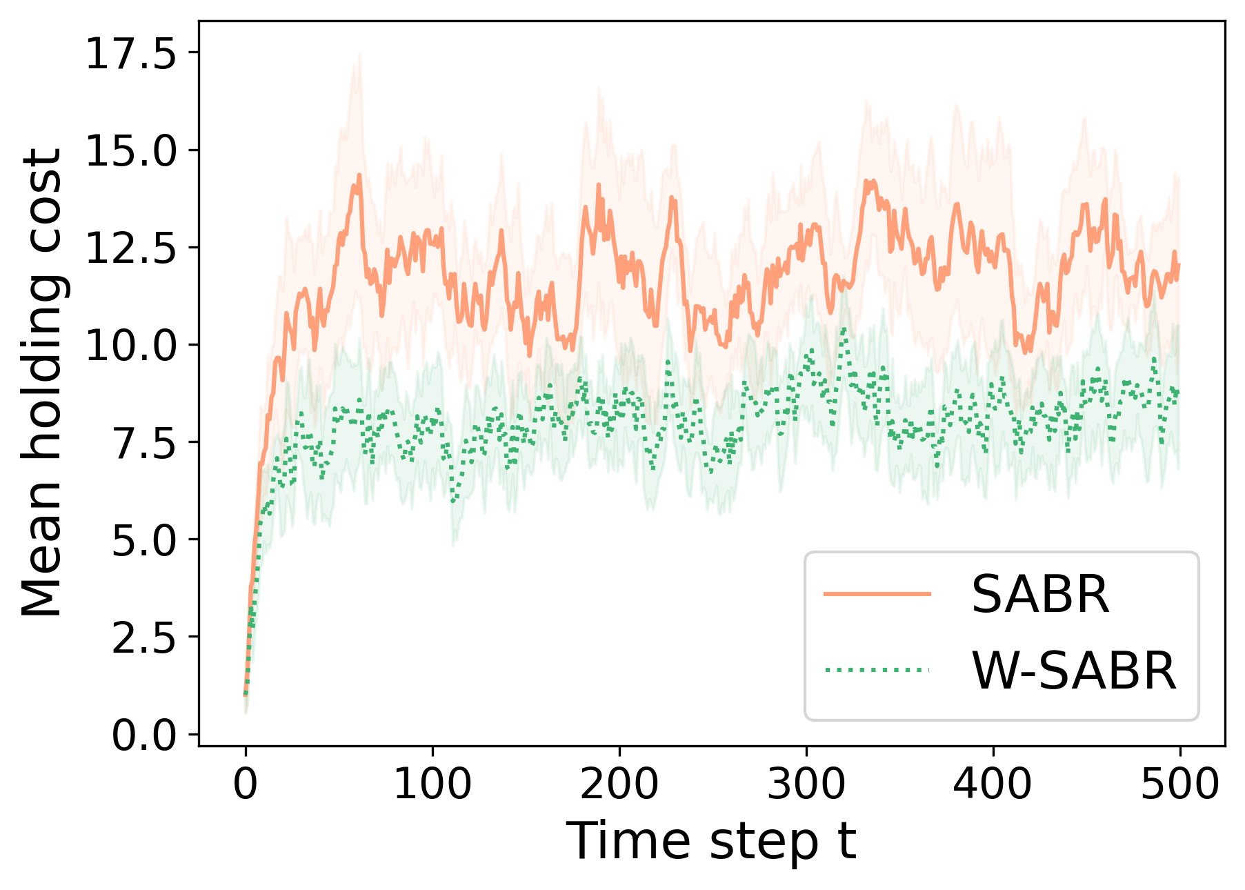
(a)

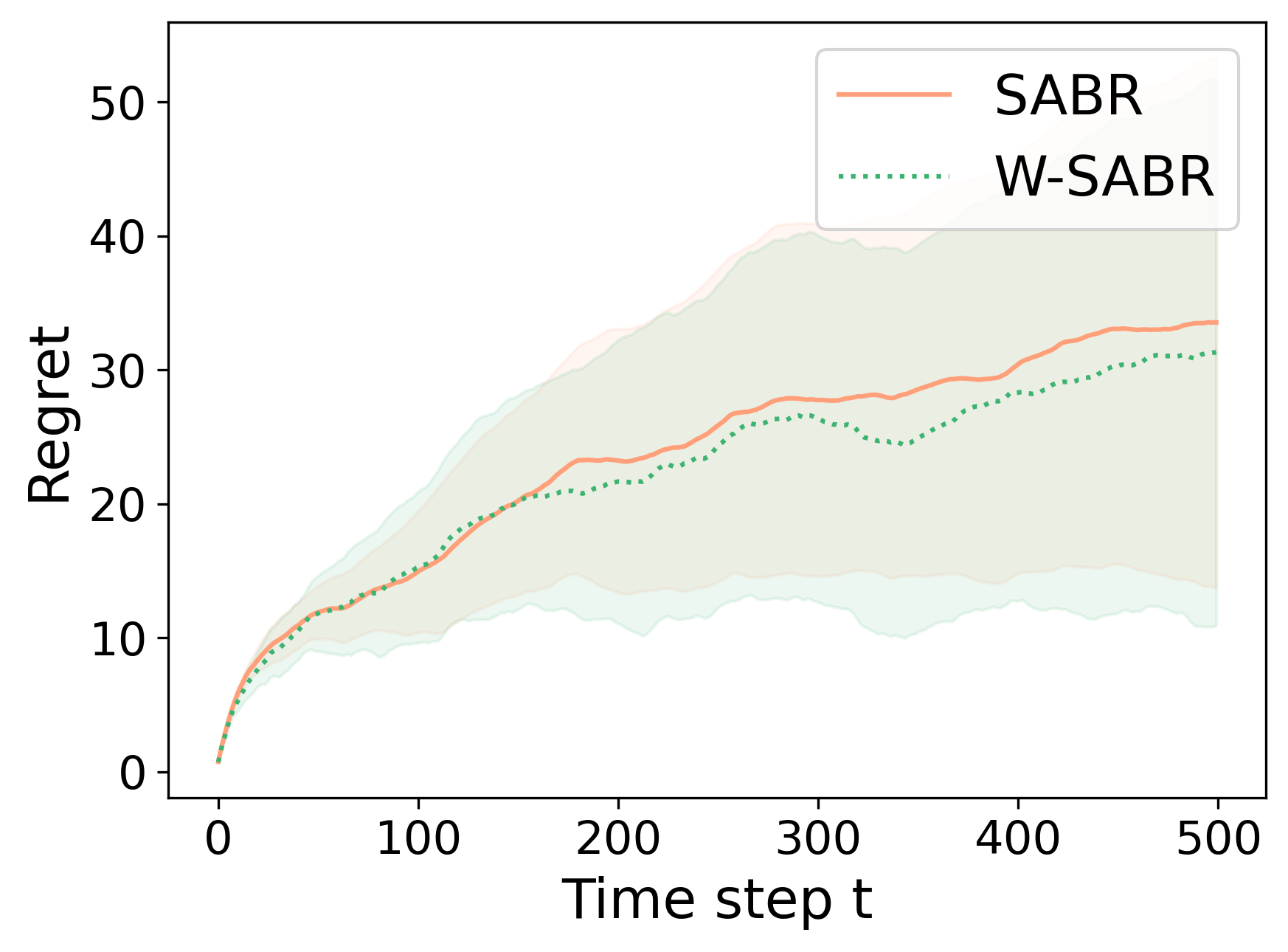
(b)

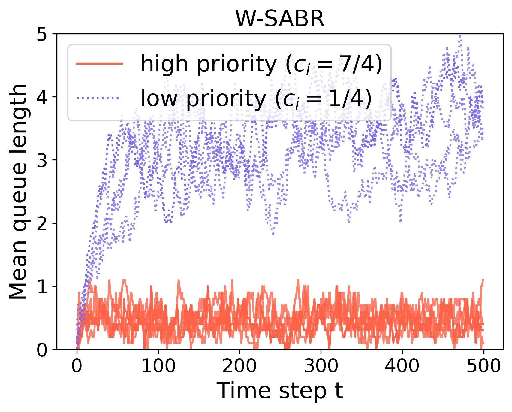
(c)

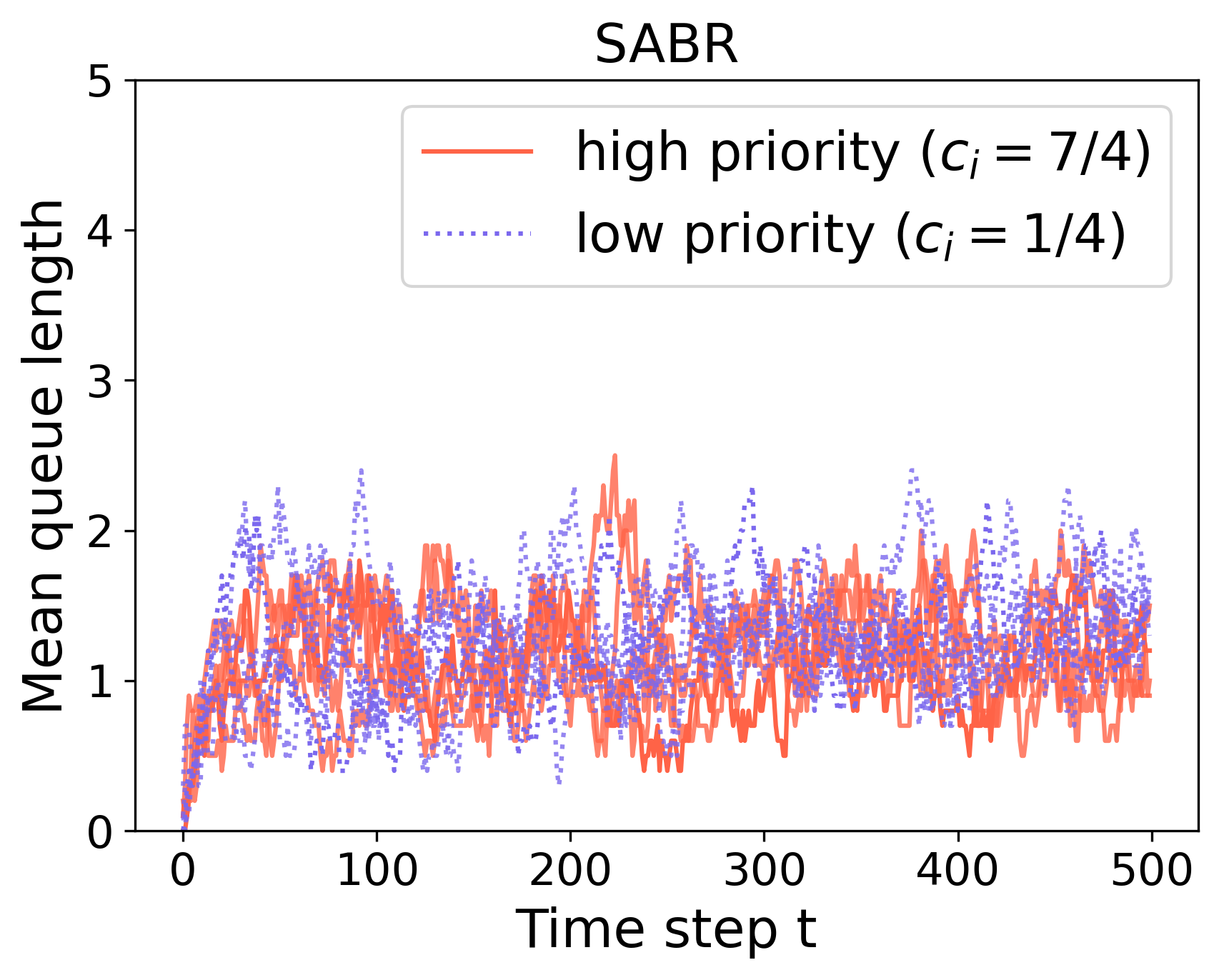
(d)

Figure 4: Mean holding cost and regret of SABR and W-SABR over time steps: (a) Mean holding cost (b) Regret (c) Mean queue length for each job class from W-SABR (d) Mean queue length for each job class from SABR.

Performance comparison.

We compare the performance of our algorithm with previously proposed algorithm in Hsu et al. (2021), which we refer to as UGDA-OL (Utility-Guided Dynamic Assignment with Online Learning). We set $T=500$, $1/\mu=1$, $I=10$, and $J=2$. Figure 3 shows that regret of SABR outperforms that of UGDA-OL which validates theoretical results. The performance gains of our algorithm come from the fact that our algorithm utilizes information acquired for a group of jobs in each class to learn reward parameters. Both algorithms achieve comparable mean queue lengths.

Mean holding costs.

We next examine how mean holding costs. We set $I=10$, $J=2$, $1/\mu=1$, and $T=500$. Marginal job holding cost parameters $c_{i}$ are set to $7/4$ for a half of job classes and to $1/4$ for remaining job classes. The job classes having $c_{i}=7/4$ can be considered as high priority jobs and the other as low priority jobs. We set $w_{i}=c_{i}$ for all $i\in\mathcal{I}$ for W-SABR and $w_{i}=1$ for all $i\in\mathcal{I}$ for SABR. In Figure 4 (a,b), W-SABR shows a lower job holding cost than SABR which is suggested by Theorem 3.3 while W-SABR and SABR show comparable regret bounds. Figure 4 (c) shows the mean queue length for each job class for W-SABR. We can observe that jobs with higher weights have smaller mean queue lengths. Finally, Figure 4 (d) for SABR shows that mean queue lengths tend to be independent of job classes as expected.

5.2 Experiments using real-world data

In this section we present numerical results for the evaluation of our proposed algorithm applied to scheduling servers in cluster computing systems. This evaluation is performed by using the dataset cluster-data-2019, which contains information about jobs and servers in the Google Borg cluster system. This dataset is available in public domain and information about the dataset is provided in https://github.com/google/cluster-data and Verma et al. (2015), Tirmazi et al. (2020). The dataset contains information about different entities, including machines, collections, and instances. Machines are servers with different CPU characteristics and memory capacities. Collections are jobs submitted to the cluster, with each job consisting of one or more tasks, referred to as instances.

For our experiments, we used the data collected over a time interval from the beginning of the trace to 5,000 seconds of the trace. There are 9,526 machines which started before the beginning of the measurement interval and 71 enqueued collections. The dataset contains information about CPU and memory capacity of each machine and CPU and memory request size for each instance. We use this information to construct feature vectors of collections and machines. For each collection, we first represent each collection with the average CPU and the average memory request size of instances of this collection, and use this to cluster collections in 5 different classes by using the K-means clustering algorithm. Each class of collections is represented by average value of CPU and memory request size of this class. For machines, we computed that there are 12 different classes of machines with respect to their CPU and memory capacities. In addition to CPU and memory (request) capacity values, we also used their inverse values, which amounts to using feature vectors of dimension $d=4$. The dataset also contain information about average number of cycles per instruction (CPI) for each assignment of an instance to a machine. The inverse CPI computed for an instance-machine combination, indicates how efficiently is the instance executed by the machine. This performance indicator depends on the characteristics of the computing that needs to be performed for given instance and characteristics of the machine. We use the inverse CPIs to define stochastic rewards of assignments. More detailed explanations for our experiments are provided in Appendix 14.

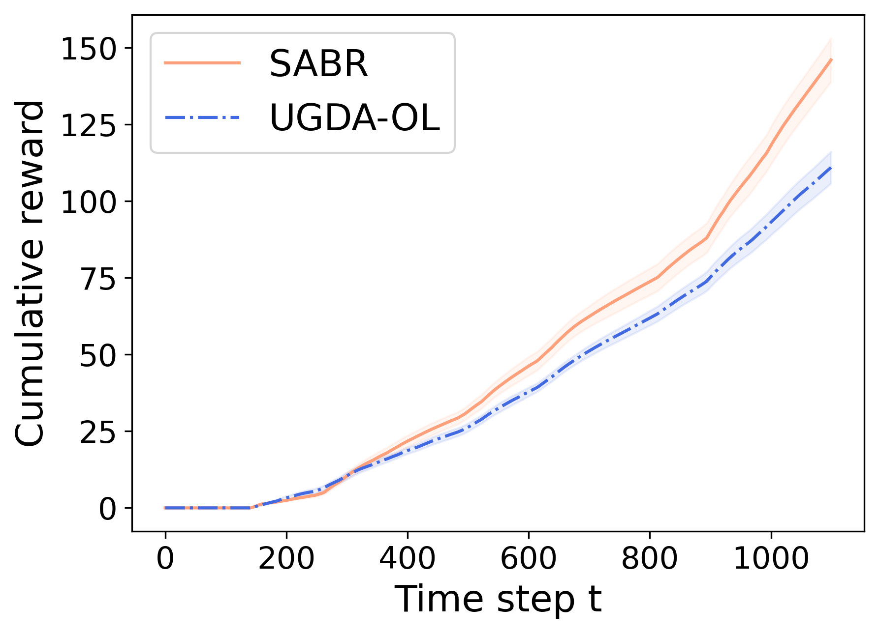
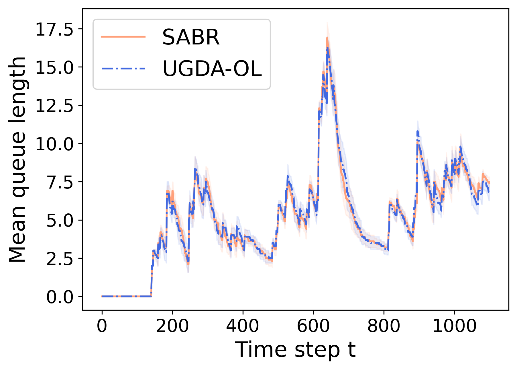
Figure 5: Performance of SABR and UGDA-OL over time steps: (left) cumulative reward and (right) mean queue length.

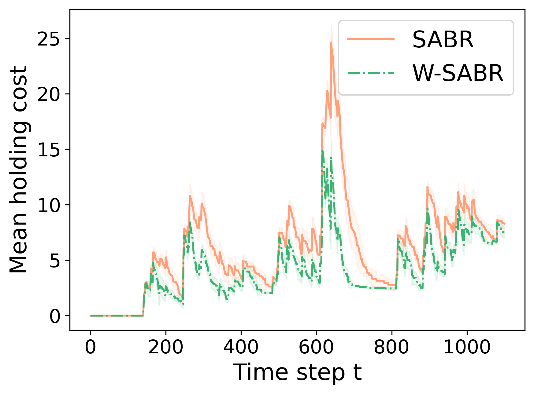
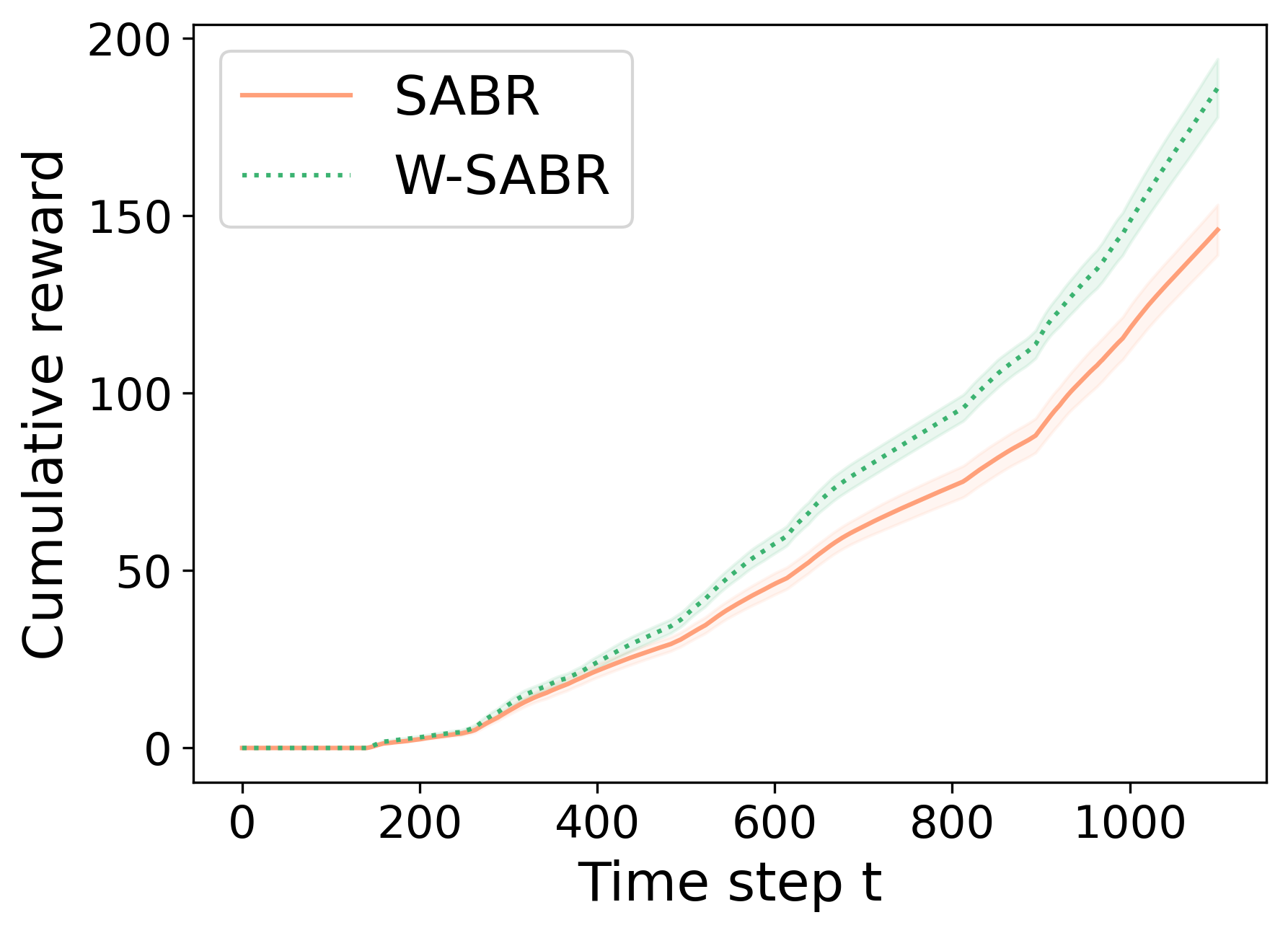
Figure 6: Mean holding cost and cumulative reward of SABR and W-SABR over time steps.

We run scheduling algorithms over discrete time steps, each 5 seconds, which amounts to $T=1100$ time steps. All instances assigned to machines in a time step are assumed to be completely processed in this time step. Each machine is allowed to be assigned at most one instance in each time step. In Figure 5, we compare the performance of our algorithm SABR with UGDA-OL for the accumulative rewards and mean queue lengths at different time steps. We observe that SABR outperforms UGDA-OL with respect to cumulative reward while the both algorithms show comparable mean queue lengths. We next examine how the mean holding cost depends on time step for SABR and W-SABR. For the job holding cost for $5$ different job classes, we set $c_{i}=7/4$ for two of the job classes for the high priority, $c_{i}=1$ for one of the job classes for the medium priority, and $c_{i}=1/4$ for the rest for the low priority. In W-SABR, we set $w_{i}=c_{i}$ and in SABR, we set $w_{i}=1$. In Figure 6, we can observe that W-SABR shows better mean holding cost and cumulative reward than SABR in most of the time steps.

6 Conclusion

We studied the problem of scheduling servers in queueing systems where assignments of jobs to servers result in stochastic rewards, with mean rewards depending on the features of jobs and servers according to a bilinear model. We proposed and studied performance of an algorithm that combines learning with scheduling for maximizing the expected reward of job-server assignments while keeping the queuing system stable and allowing for different job priorities. This algorithm uses a learning procedure for estimating rewards of job-server assignments that accounts for the exploration versus exploitation trade-off. We have shown that the regret of our proposed algorithm scales sublinearly with the time horizon, the number of job classes, and is independent of the number of server classes. This improves upon a previously known linearly increasing regret bound with the horizon time achieved by an algorithm that makes no structural assumptions about mean rewards and their relation with job and server features and, hence, amounts to learning expected rewards of assignments for each job separately. We derived bounds under various assumptions, allowing for non-identical mean job service times and a time-varying set of server classes. We have discussed how our proposed algorithm can be distributed which is of interest for implementation in large-scale systems.

There are several directions for future research. First, our regret bounds scale quadratically with the number of servers, as in previous work, which may be improved. This could be either by using a different algorithm or a more refined analysis. Second, the regret bounds scale quadratically with the dimension of feature vectors representing jobs and servers, which may be improved by assuming a bilinear model with a low-rank parameter. Finally, for the case allowing for non-identical mean job service times, our regret and mean queue length bounds hold under a stability condition that could be relaxed.

7 Appendix

8 Proof of Theorem 3.1

We first provide an outline of the proof to highlight the main steps and then a detailed proof.

8.1 Proof outline

The proof is based on decomposing the regret into different components that amounts to the following regret bound

$$R(T) \leq\gamma\frac{1}{\mu}\mathbb{E}[Q(T)]+\frac{1}{V}\sum_{t=1}^{T}\mathbb{E}\left[G(t)\right]+\frac{1}{V}\left(\sum_{t=1}^{T}\mathbb{E}\left[H(t)\right]+\frac{1}{2}\left(\sum_{i\in\mathcal{I}}w_{i}\right)(T+1)\right),$$ (26)

where

$$G(t)=\sum_{i\in\mathcal{I}(t)}\sum_{j\in\mathcal{J}}\left(\frac{w_{i}}{\rho_{i}}Q_{i}(t)+V(r_{i,j}-\gamma)\right)\left(\rho p_{i,j}^{*}-y_{i,j}(t)\right)$$

and

$$H(t)=\frac{n^{2}}{2}\left(1+c_{a,\gamma}^{2}\mu\right)\left(\max_{i\in\mathcal{I}(t)}\frac{w_{i}}{\rho_{i}}\right).$$

For showing (26), we use the drift-plus-penalty method with the Lyapunov function defined as

$$L({q})=\frac{1}{2}\sum_{i\in\mathcal{I}}\frac{w_{i}}{\rho_{i}}q_{i}^{2}.$$

Let

$$\Delta(t) =\sum_{i\in\mathcal{I}}\rho_{i}\sum_{j\in\mathcal{J}}p_{i,j}^{*}(r_{i,j}-\gamma)-\sum_{i\in\mathcal{I}(t)}\sum_{j\in\mathcal{J}}y_{i,j}(t)(r_{i,j}-\gamma).$$ (27)

By analyzing the drift-plus-penalty function, we can obtain

$$\mathbb{E}\left[L({Q}(t+1))-L({Q}(t))+V\mu\Delta(t)\right]\leq\mu\mathbb{E}\left[G(t)\right]+\mu\mathbb{E}[H(t)]+\frac{\mu}{2}\sum_{i\in\mathcal{I}}w_{i},$$ (28)

from which (26) easily follows.

The regret bound in (26) consists of three components, the first component is proportional to the mean queue length, the second component is due to the bandit learning algorithm, and finally, the third component is due to stochasticity of job arrivals and departures.

The term $G(t)$ is the key term for bounding the effect of the bandit learning algorithm on regret. Denote by $(y^{*}_{i,j}(t),i\in\mathcal{I}(t),j\in\mathcal{J})$ the solution of the optimization problem (4) with parameters $\hat{r}_{i,j}$ replaced with the true mean values $r_{i,j}$. Then, it can be shown that

$$G(t)\leq G_{1}(t)+G_{2}(t),$$

where $G_{1}(t)=V\sum_{i\in\mathcal{I}(t)}\sum_{j\in\mathcal{J}}(\hat{r}_{i,j}(t)-r_{i,j})y_{i,j}(t)$ and $G_{2}(t)=V\sum_{i\in\mathcal{I}(t)}\sum_{j\in\mathcal{J}}(r_{i,j}-\hat{r}_{i,j}(t))y^{*}_{i,j}(t).$ Note that $G_{1}(t)$ and $G_{2}(t)$ are weighted sums of mean reward estimation errors. In our setting, rewards are according to the bilinear model, which makes the analysis different from that in Hsu et al. (2021). Note also that multiple jobs may need to be assigned to multiple servers at each time step, which makes the regret analysis different from previous work on bandit algorithms (Abbasi-Yadkori et al. 2011). For analyzing the regret under the bilinear model, as standard, we convert it to a linear model. We explain this in more details as follows.

To provide a bound for the weighted sums of the mean reward estimation errors, we consider the error of the estimator of $\theta$ by using a weighted norm. Let $x_{\upsilon(k),j}(t)=y_{\upsilon(k),j}(t)/Q_{\upsilon(k)}(t)$ and $\tilde{x}_{\upsilon(k),j}(t)$ be the actual number of servers of class $j$ assigned to job $k$ in time step $t$ such that $\mathbb{E}[\tilde{x}_{\upsilon(k),j}(t)\mid x_{\upsilon(k),j}(t)]=x_{\upsilon(k),j}(t)$, and $\tilde{\mathcal{Q}}(t)$ be the set of assigned jobs in $\mathcal{Q}(t)$ to servers at time $t$. Let $\hat{\theta}_{i,j}(t)=\hat{\theta}(t)+\Delta^{*}_{i,j}(t)$, where recall $\Delta^{*}_{i,j}(t)$ is defined in (11). Then, we can show that

$$\frac{1}{V}\sum_{t=1}^{T}\mathbb{E}\left[G_{1}(t)\right] =\sum_{t=1}^{T}\mathbb{E}\left[\sum_{i\in\mathcal{I}(t),j\in J}(\hat{r}_{i,j}(t)-r_{i,j})y_{i,j}(t)\right]$$ (29)

$$=\sum_{t=1}^{T}\mathbb{E}\left[\sum_{k\in\mathcal{Q}(t),j\in J}(\hat{r}_{\upsilon(k),j}(t)-r_{\upsilon(k),j})x_{\upsilon(k),j}(t)\right]$$ (30)

$$=\sum_{t=1}^{T}\mathbb{E}\left[\sum_{k\in\tilde{\mathcal{Q}}(t),j\in\mathcal{J}}(\hat{r}_{\upsilon(k),j}(t)-r_{\upsilon(k),j})\tilde{x}_{\upsilon(k),j}(t)\right]$$ (31)

$$\leq\sum_{t=1}^{T}\mathbb{E}\left[\sum_{k\in\tilde{\mathcal{Q}}(t),j\in\mathcal{J}}\|w_{\upsilon(k),j}\|_{\Lambda(t)^{-1}}\cdot\|\hat{\theta}_{\upsilon(k),j}(t)-\theta\|_{\Lambda(t)}\tilde{x}_{\upsilon(k),j}(t)\right]$$ (32)

$$\leq\sum_{t=1}^{T}\mathbb{E}\left[\sum_{k\in\tilde{\mathcal{Q}}(t),j\in\mathcal{J}}\|w_{\upsilon(k),j}\|_{\Lambda(t)^{-1}}\sqrt{\beta(t)}\tilde{x}_{\upsilon(k),j}(t)\right].$$ (33)

By conditioning on the event $\{\theta\in{\mathcal{C}}(t)$ for $t\in\mathcal{T}\}$, which holds with high probability, we have

$$\sum_{t=1}^{T}\sum_{k\in\tilde{\mathcal{Q}}(t),j\in\mathcal{J}}(\hat{r}_{\upsilon(k),j}(t)-r_{\upsilon(k),j})\tilde{x}_{\upsilon(k),j}(t)$$ (34)

$$\leq\sum_{t=1}^{T}\sum_{k\in\tilde{\mathcal{Q}}(t),j\in\mathcal{J}}\|w_{\upsilon(k),j}\|_{\Lambda(t)^{-1}}\cdot\|\hat{\theta}_{\upsilon(k),j}(t)-\theta\|_{\Lambda(t)}\tilde{x}_{\upsilon(k),j}(t)$$ (35)

$$\leq\sum_{t=1}^{T}\sum_{k\in\tilde{\mathcal{Q}}(t),j\in\mathcal{J}}\|w_{\upsilon(k),j}\|_{\Lambda(t)^{-1}}\sqrt{\beta(t)}\tilde{x}_{\upsilon(k),j}(t),$$ (36)

where the second inequality is obtained by using the fact $\theta\in{\mathcal{C}}(t)$.

By leveraging Lemma 4.2 in Qin et al. (2014) with some adjustments, we can show that

$$\sum_{t=1}^{T}\sum_{k\in\tilde{\mathcal{Q}}(t),j\in\mathcal{J}}\tilde{x}_{\upsilon(k),j}(t)\|w_{\upsilon(k),j}\|_{\Lambda(t)^{-1}}^{2}\leq 2d^{2}\log\left(n+\frac{n}{d^{2}}T\right).$$ (37)

Recall that $\sqrt{\beta(t)}=\kappa\sqrt{d^{2}\log(tT)}+\sqrt{n}$ for a constant $\kappa\geq 0$. Then, by using (33), (36), (37), and the Cauchy-Schwarz inequality, we obtain

$$\frac{1}{V}\sum_{t=1}^{T}\mathbb{E}\left[G_{1}(t)\right]\leq\mathbb{E}\left[\sqrt{nT\beta(T)\sum_{t=1}^{T}\sum_{k\in\tilde{\mathcal{Q}}(t),j\in\mathcal{J}}\tilde{x}_{\upsilon(k),j}(t)\|w_{\upsilon(k),j}\|_{\Lambda(t)^{-1}}^{2}}\right]+2an=\tilde{O}(ad^{2}\sqrt{nT}+adn\sqrt{T}).$$

It can be further established that $(1/V)\sum_{t=1}^{T}\mathbb{E}[G_{2}(t)]\leq 2an$. Hence, it follows

$$\frac{1}{V}\sum_{t=1}^{T}\mathbb{E}[G_{1}(t)]+\frac{1}{V}\sum_{t=1}^{T}\mathbb{E}[G_{2}(t)]=\tilde{O}(a(\sqrt{n}d^{2}+nd)\sqrt{T}).$$ (38)

Note that $(1/V)\sum_{t=1}^{T}\mathbb{E}[G_{1}(t)]$ dominates $(1/V)\sum_{t=1}^{T}\mathbb{E}[G_{2}(t)]$ because $(1/V)\sum_{t=1}^{T}G_{2}(t)$ is negative with high probability, which follows from the definition of the mean reward estimators.

From (26) and (38), and the mean queue length bound in Theorem 15, we obtain the regret bound assserted in Theorem 3.1.

8.2 Proof of the theorem

The proof uses a regret bound that has three components and then proceeds with separately bounding these components. The first component is proportional to the mean queue length. The second component is due to the bandit learning algorithm. This term is bounded by leveraging the bilinear structure of rewards. The third component is due to randomness of job arrivals and departures. In the following lemma, we provide a regret bound that consists of the three aforementioned components.

Lemma 8.1

The regret is bounded as follows

$$R(T) \leq\gamma\frac{1}{\mu}\mathbb{E}[Q(T)]+\frac{1}{V}\sum_{t=1}^{T}\mathbb{E}\left[G(t)\right]+\frac{1}{V}\left(\sum_{t=1}^{T}\mathbb{E}\left[H(t)\right]+\frac{1}{2}\left(\sum_{i\in\mathcal{I}}w_{i}\right)(T+1)\right),$$

where

$$G(t)=\sum_{i\in\mathcal{I}(t)}\sum_{j\in\mathcal{J}}\left(\frac{w_{i}}{\rho_{i}}Q_{i}(t)+V(r_{i,j}-\gamma)\right)\left(\rho_{i}p_{i,j}^{*}-y_{i,j}(t)\right)$$

and

$$H(t)=\frac{n^{2}}{2}\left(1+c_{a,\gamma}^{2}\mu\right)\left(\max_{i\in\mathcal{I}(t)}\frac{w_{i}}{\rho_{i}}\right).$$

Proof 8.2

Proof. The queues of different job classes $i\in\mathcal{I}$ evolve as

$$Q_{i}(t+1)=Q_{i}(t)+A_{i}(t+1)-D_{i}(t),$$

where $A_{i}(t+1)$ and $D_{i}(t)$ are the number of class-$i$ job arrivals at the beginning of time step $t+1$ and the number of class-$i$ job departures at the end of time step $t$, respectively. Let $A(t)=\sum_{i\in\mathcal{I}}A_{i}(t)$ and $D(t)=\sum_{i\in\mathcal{I}}D_{i}(t).$

We use the Lyapunov function defined as

$$L({q})=\frac{1}{2}\sum_{i\in\mathcal{I}}\frac{w_{i}}{\rho_{i}}q_{i}^{2}.$$

The following conditional expected drift equations hold for queues of different job classes: if $i\notin\mathcal{I}(t)$,

$$\mathbb{E}[Q_{i}(t+1)^{2}-Q_{i}(t)^{2}\mid Q_{i}(t)=0]=\mathbb{E}[A_{i}(t+1)^{2}]=\lambda_{i},$$

and, otherwise, if $i\in\mathcal{I}(t)$,

$$\mathbb{E}[Q_{i}(t+1)^{2}-Q_{i}(t)^{2}\mid\mathcal{Q}(t),{x}(t)]$$ (39)

$$\leq\mathbb{E}[2Q_{i}(t)(A_{i}(t+1)-D_{i}(t))+(A_{i}(t+1)-D_{i}(t))^{2})\mid\mathcal{Q}(t),{x}(t)]$$ (40)

$$\leq 2Q_{i}(t)\left(\lambda_{i}-\mathbb{E}[D_{i}(t)\mid\mathcal{Q}(t),{x}(t)]\right)+\lambda_{i}+\mathbb{E}[D_{i}(t)^{2}\mid\mathcal{Q}(t),{x}(t)].$$ (41)

We next derive bounds for $\mathbb{E}[D_{i}(t)\mid\mathcal{Q}(t),{x}(t)]$ and $\mathbb{E}[D_{i}(t)^{2}\mid\mathcal{Q}(t),{x}(t)]$ in the following lemma. The proof of the lemma follows the proof steps of Lemma EC.7 in Hsu et al. (2021), with some adjustments to allow for weighted proportional fair allocation.

Lemma 8.3

For any $i\in\mathcal{I}(t)$, we have

$$\mathbb{E}[D_{i}(t)\mid\mathcal{Q}(t),y(t)]\geq\mu\sum_{j\in\mathcal{J}}y_{i,j}(t)-\frac{\mu^{2}n^{2}(\gamma+a)^{2}}{2(\gamma-a)^{2}}\frac{w_{i}^{2}Q_{i}(t)}{\sum_{i^{\prime}\in\mathcal{I}(t)}w_{i^{\prime}}^{2}Q_{i^{\prime}}(t)^{2}}.$$

and

$$\sum_{i^{\prime}\in\mathcal{I}}\mathbb{E}[D_{i^{\prime}}(t)^{2}\mid\mathcal{Q}(t),y(t)]\leq n^{2}\mu.$$

Proof 8.4

Proof. Let $E_{i}(t)$ be the event that job $k\in\mathcal{Q}_{i}(t)$ for $i\in\mathcal{I}(t)$ is not completed at the end of time step $t$. A server of class $j$ is assigned job $k$ with probability $y_{i,j}(t)/(n_{j}Q_{i}(t))$, and this job is completed with probability $\mu$ by the memory-less property of geometric distribution. Therefore, we have

$$\mathbb{P}[E_{i}(t)\mid\mathcal{Q}(t),y(t)]=\prod_{j\in\mathcal{J}}\left(1-\mu\frac{y_{i,j}(t)}{n_{j}Q_{i}(t)}\right)^{n_{j}},$$ (42)

and

$$\mathbb{E}[D_{i}(t)|{\mathcal{Q}}(t),y(t)]=\sum_{k\in\mathcal{Q}_{i}(t)}\left(1-\mathbb{P}[E_{i}(t)\mid\mathcal{Q}(t),y(t)]\right)=Q_{i}(t)\left(1-\mathbb{P}[E_{i}(t)\mid\mathcal{Q}(t),y(t)]\right).$$

Using $1-x\leq e^{-x}\leq 1-x+x^{2}/2$ for $x\geq 0$, we have

$$1-\mathbb{P}[E_{i}(t)\mid\mathcal{Q}(t),y(t)] \geq 1-\exp\left(-\sum_{j\in\mathcal{J}}\mu\frac{y_{i,j}(t)}{Q_{i}(t)}\right)$$

$$\geq \mu\sum_{j\in\mathcal{J}}\frac{y_{i,j}(t)}{Q_{i}(t)}-\frac{\mu^{2}}{2}\left(\sum_{j\in\mathcal{J}}\frac{y_{i,j}(t)}{Q_{i}(t)}\right)^{2}.$$

Hence, for any $i\in\mathcal{I}(t)$ we have

$$\mathbb{E}[D_{i}(t)\mid\mathcal{Q}(t),y(t)]\geq\mu\sum_{j\in\mathcal{J}}y_{i,j}(t)-\frac{\mu^{2}}{2}\frac{1}{Q_{i}(t)}\left(\sum_{j\in\mathcal{J}}y_{i,j}(t)\right)^{2}.$$ (43)

Let $q(t)=(q_{j}(t),j\in\mathcal{J})\in\mathbb{R}_{+}^{J}$ be the Lagrange multipliers for the constraints $\sum_{i\in\mathcal{I}(t)}y_{i,j}(t)\leq n_{j}$ for all $j\in\mathcal{J}$ and $h(t)=(h_{i,j}(t),i\in\mathcal{I}(t),j\in\mathcal{J})\in\mathbb{R}_{+}^{|\mathcal{I}(t)|\times J}$ be the Lagrange multipliers for the constraints $y_{i,j}(t)\geq 0$ for all $i\in\mathcal{I}(t)$ and $j\in\mathcal{J}$ in $\eqref{eq:weighted}$. Then, we have the Lagrangian function for the optimization problem (4) given as

$$\mathcal{L}(y(t),q(t),h(t)) =\sum_{i\in\mathcal{I}(t)}\left[\frac{1}{V}Q_{i}(t)w_{i}\log\left(\sum_{j\in\mathcal{J}}y_{i,j}(t)\right)+\sum_{j\in\mathcal{J}}y_{i,j}(t)(\hat{r}_{i,j}(t)-\gamma)\right]$$

$$\qquad+\sum_{j\in\mathcal{J}}q_{j}(t)\left(n_{j}-\sum_{i\in\mathcal{I}(t)}y_{i,j}(t)\right)+\sum_{i\in\mathcal{I}(t),j\in\mathcal{J}}h_{i,j}(t)y_{i,j}(t).$$

If $y(t)$ is a solution of (4), then $y(t)$ satisfies the following stationarity conditions,

$$\sum_{j^{\prime}\in\mathcal{J}}y_{i,j^{\prime}}(t)=\frac{1}{V}\frac{w_{i}Q_{i}(t)}{q_{j}(t)-h_{i,j}(t)+\gamma-\hat{r}_{i,j}(t)},\hbox{ for all }i\in\mathcal{I}(t),$$ (44)

and the following complementary slackness conditions,

$$q_{j}(t)\left(n_{j}-\sum_{i\in\mathcal{I}(t)}y_{i,j}(t)\right)=0,\hbox{ for all }j\in\mathcal{J}$$ (45)

and

$$h_{i,j}(t)y_{i,j}(t)=0,\hbox{ for all }i\in\mathcal{I}(t),j\in\mathcal{J}.$$ (46)

The convex optimization problem in (4), with $n_{j}>0$ for all $j\in\mathcal{J}$, always has a feasible solution. This implies that for any $i\in\mathcal{I}(t)$, there exists $j_{0}\in\mathcal{J}$ such that $y_{i,j_{0}}(t)>0$ since $\sum_{j\in\mathcal{J}}y_{i,j}(t)>0$ from $\log(\sum_{j\in\mathcal{J}}y_{i,j}(t))$ in (4). This implies that $h_{i,j_{0}}(t)=0$ from the complementary slackness conditions (46). Consider any two job classes $i$ and $i^{\prime}$ in $\mathcal{I}(t)$. We have

$$q_{j}(t)+\gamma-\hat{r}_{i,j}(t)\geq q_{j}(t)+\gamma-a\geq\frac{\gamma-a}{\gamma+a}(q_{j}(t)+\gamma-\hat{r}_{i^{\prime},j}(t)).$$ (47)

From (44), (46), and (47), we have

$$\sum_{j\in\mathcal{J}}y_{i,j}(t) =\frac{w_{i}Q_{i}(t)}{V(q_{j_{0}}(t)-h_{i,j_{0}}(t)+\gamma-\hat{r}_{i,j_{0}}(t))}$$ (48)

$$=\frac{w_{i}Q_{i}(t)}{V(q_{j_{0}}(t)+\gamma-\hat{r}_{i,j_{0}}(t))}$$ (49)

$$\leq\frac{w_{i}Q_{i}(t)(\gamma+a)/(\gamma-a)}{V(q_{j_{0}}(t)+\gamma-\hat{r}_{i^{\prime},j_{0}}(t))}$$ (50)

$$\leq\frac{w_{i}Q_{i}(t)}{w_{i^{\prime}}Q_{i^{\prime}}(t)}\frac{w_{i^{\prime}}Q_{i^{\prime}}(t)(\gamma+a)/(\gamma-a)}{V(q_{j_{0}}(t)-h_{i^{\prime},j_{0}}(t)+\gamma-\hat{r}_{i^{\prime},j_{0}}(t))}$$ (51)

$$\leq\frac{w_{i}Q_{i}(t)}{w_{i^{\prime}}Q_{i^{\prime}}(t)}\frac{\gamma+a}{\gamma-a}\sum_{j\in\mathcal{J}}y_{i^{\prime},j}(t).$$ (52)

From (52), we have

$$n \geq\sum_{i^{\prime}\in\mathcal{I}(t)}\sum_{j\in\mathcal{J}}y_{i^{\prime},j}(t)$$ (53)

$$\geq((\gamma-a)/(\gamma+a))\sum_{i^{\prime}\in\mathcal{I}(t)}\frac{w_{i^{\prime}}Q_{i^{\prime}}(t)}{w_{i}Q_{i}(t)}\sum_{j\in\mathcal{J}}y_{i,j}(t).$$ (54)

Then, from (43) and (54), we obtain

$$\mathbb{E}[D_{i}(t)\mid\mathcal{Q}(t),y(t)] \geq\mu\sum_{j\in\mathcal{J}}y_{i,j}(t)-\frac{\mu^{2}}{2}\frac{1}{Q_{i}(t)}\left(\sum_{j\in\mathcal{J}}y_{i,j}(t)\right)^{2}$$

$$\geq\mu\sum_{j\in\mathcal{J}}y_{i,j}(t)-\frac{\mu^{2}n^{2}(\gamma+a)^{2}}{2(\gamma-a)^{2}}\frac{w_{i}^{2}Q_{i}(t)}{\sum_{i^{\prime}\in\mathcal{I}(t)}w_{i^{\prime}}^{2}Q_{i^{\prime}}(t)^{2}}.$$

Applying $(1-x)(1-y)\geq 1-(x+y)$ for all $x,y\geq 0$, from (42) we obtain

$$\mathbb{E}[D_{i}(t)\mid\mathcal{Q}(t),y(t)]=Q_{i}(t)\left(1-\mathbb{P}[E_{i}(t)\mid\mathcal{Q}(t),y(t)]\right)\leq\mu\sum_{j\in J}y_{i,j}(t).$$ (55)

From (55) and $D_{i}(t)\leq\sum_{j\in\mathcal{J}}n_{j}=n$, we also have

$$\sum_{i\in\mathcal{I}}\mathbb{E}[D_{i}(t)^{2}\mid\mathcal{Q}(t),{x}(t)]\leq\sum_{i\in\mathcal{I}}\mathbb{E}[D_{i}(t)\mid\mathcal{Q}(t),{x}(t)]n\leq n^{2}\mu.$$

From (41), it follows

$$\mathbb{E}[L({Q}(t+1))-L({Q}(t))\mid\mathcal{Q}(t),{x}(t)]$$

$$\leq\sum_{i\in\mathcal{I}(t)}\left(\frac{w_{i}}{\rho_{i}}Q_{i}(t)\mu\sum_{j\in\mathcal{J}}\left(\rho_{i}p_{i,j}^{*}-y_{i,j}(t)\right)+\frac{w_{i}\lambda_{i}}{2\rho_{i}}+\frac{w_{i}}{2\rho_{i}}\mathbb{E}[D_{i}(t)^{2}\mid\mathcal{Q}(t),{x}(t)]\right)$$

$$\qquad+\frac{(\gamma+a)^{2}n^{2}\mu^{2}}{2(\gamma-a)^{2}}\left(\max_{i\in\mathcal{I}(t)}\frac{w_{i}}{\rho_{i}}\right)+\sum_{i\notin\mathcal{I}(t)}\frac{w_{i}\lambda_{i}}{2\rho_{i}}$$

$$\leq\sum_{i\in\mathcal{I}(t)}\sum_{j\in\mathcal{J}}\left(\frac{w_{i}}{\rho_{i}}Q_{i}(t)\mu\left(\rho_{i}p_{i,j}^{*}-y_{i,j}(t)\right)\right)+\frac{\mu\sum_{i\in\mathcal{I}}w_{i}}{2}+\left(\frac{(\gamma+a)^{2}n^{2}\mu^{2}}{2(\gamma-a)^{2}}+\frac{n^{2}\mu}{2}\right)\left(\max_{i\in\mathcal{I}(t)}\frac{w_{i}}{\rho_{i}}\right).$$

Note that

$$\Delta(t) =\sum_{i\in\mathcal{I}}\rho_{i}\sum_{j\in\mathcal{J}}p_{i,j}^{*}(r_{i,j}-\gamma)-\sum_{i\in\mathcal{I}(t)}\sum_{j\in\mathcal{J}}y_{i,j}(t)(r_{i,j}-\gamma)$$

$$\leq\sum_{i\in\mathcal{I}(t)}\rho_{i}\sum_{j\in\mathcal{J}}p_{i,j}^{*}(r_{i,j}-\gamma)-\sum_{i\in\mathcal{I}(t)}\sum_{j\in\mathcal{J}}y_{i,j}(t)(r_{i,j}-\gamma)$$

$$=\sum_{i\in\mathcal{I}(t)}\sum_{j\in\mathcal{J}}(r_{i,j}-\gamma)(\rho_{i}p_{i,j}^{*}-y_{i,j}(t)).$$

It follows that

$$\mathbb{E}\left[L({Q}(t+1))-L({Q}(t))+V\mu\Delta(t)\right]\leq\mu\mathbb{E}\left[G(t)\right]+\mu\mathbb{E}\left[H(t)\right]+\mu\frac{1}{2}\sum_{i\in\mathcal{I}}w_{i},$$ (56)

where

$$G(t) =\sum_{i\in\mathcal{I}(t)}\sum_{j\in\mathcal{J}}\left(\frac{w_{i}}{\rho_{i}}Q_{i}(t)+V(r_{i,j}-\gamma)\right)\left(\rho_{i}p_{i,j}^{*}-y_{i,j}(t)\right)$$

and

$$H(t)=\frac{n^{2}}{2}\left(1+\left(\frac{\gamma+a}{\gamma-a}\right)^{2}\mu\right)\left(\max_{i\in\mathcal{I}(t)}\frac{w_{i}}{\rho_{i}}\right).$$

Now, note

$$\sum_{t=1}^{T}\left(\sum_{i\in\mathcal{I}}\rho_{i}-\mathbb{E}\left[\sum_{i\in\mathcal{I}(t)}\sum_{j\in\mathcal{J}}y_{i,j}(t)\right]\right) \leq \sum_{t=1}^{T}\left(\rho-\frac{1}{\mu}\mathbb{E}[D(t)]\right)$$

$$= \frac{1}{\mu}\sum_{t=1}^{T}\mathbb{E}[A(t+1)-D(t)]$$

$$= \frac{1}{\mu}\sum_{t=1}^{T}\mathbb{E}[Q(t+1)-Q(t)]$$

$$= \frac{1}{\mu}(\mathbb{E}[Q(T+1)]-\mathbb{E}[Q(1)])$$

$$= \frac{1}{\mu}\mathbb{E}[Q(T)-D(T)+A(T+1)-A(1)]$$

$$\leq \frac{1}{\mu}\mathbb{E}[Q(T)]$$

where the first inequality is from (55). Note also that

$$\sum_{t=1}^{T}\mathbb{E}[\Delta(t)] =\sum_{t=1}^{T}\left(\mathbb{E}\left[\sum_{i\in\mathcal{I}}\sum_{j\in\mathcal{J}}\rho_{i}r_{i,j}p_{i,j}^{*}-\sum_{i\in\mathcal{I}(t)}\sum_{j\in\mathcal{J}}r_{i,j}y_{i,j}(t)\right]\right)-\gamma\sum_{t=1}^{T}\left(\rho-\mathbb{E}\left[\sum_{i\in\mathcal{I}(t)}\sum_{j\in\mathcal{J}}y_{i,j}(t)\right]\right)$$ (57)

$$\geq\sum_{t=1}^{T}\left(\sum_{i\in\mathcal{I}}\sum_{j\in\mathcal{J}}\rho_{i}r_{i,j}p_{i,j}^{*}-\mathbb{E}\left[\sum_{i\in\mathcal{I}(t)}\sum_{j\in\mathcal{J}}r_{i,j}y_{i,j}(t))\right]\right)-\gamma\frac{1}{\mu}\mathbb{E}[Q(T)]$$ (58)

$$=R(T)-\gamma\frac{1}{\mu}\mathbb{E}[Q(T)].$$ (59)

From (56) and (59), and using the facts

$$\mathbb{E}[L({Q}(1))]=\frac{1}{2}\mathbb{E}\left[\sum_{i\in\mathcal{I}}\frac{w_{i}}{\rho_{i}}Q_{i}(1)^{2}\right]=\frac{1}{2}\mathbb{E}\left[\sum_{i\in\mathcal{I}}\frac{w_{i}}{\rho_{i}}A_{i}(1)^{2}\right]=\frac{\mu\sum_{i\in\mathcal{I}}w_{i}}{2}$$

and $L({Q}(T+1))\geq 0$, we have

$$R(T) =\sum_{t=1}^{T}\left(\sum_{i\in\mathcal{I}}\sum_{j\in\mathcal{J}}\rho_{i}r_{i,j}p_{i,j}^{*}-\mathbb{E}\left[\sum_{i\in\mathcal{I}(t)}\sum_{j\in\mathcal{J}}r_{i,j}y_{i,j}(t)\right]\right)$$

$$\leq\gamma\frac{1}{\mu}\mathbb{E}[Q(T)]+\frac{1}{V}\sum_{t=1}^{T}\mathbb{E}[G(t)]+\frac{1}{V}\left(\sum_{t=1}^{T}\mathbb{E}[H(t)]+(T+1)\frac{1}{2}\sum_{i\in\mathcal{I}}w_{i}\right).$$

In what follows we focus on bounding the regret component which is due the bandit learning algorithm. Denote by $y^{*}(t)=(y^{*}_{i,j}(t),i\in\mathcal{I}(t),j\in\mathcal{J})$ the solution of the optimization problem (4) with the mean reward estimates $\hat{r}_{i,j}$ replaced with the true mean rewards $r_{i,j}$. We use a bound for $G(t)$ in terms of two variables quantifying the gap between true and estimated mean rewards as given in the following lemma. This lemma was established in Hsu et al. (2021).

Lemma 8.5

The following bound holds for all $t\geq 1$,

$$G(t)\leq G_{1}(t)+G_{2}(t),$$

where

$$G_{1}(t)=V\sum_{i\in\mathcal{I}(t)}\sum_{j\in\mathcal{J}}(\hat{r}_{i,j}(t)-r_{i,j})y_{i,j}(t),$$

and

$$G_{2}(t)=V\sum_{i\in\mathcal{I}(t)}\sum_{j\in\mathcal{J}}(r_{i,j}-\hat{r}_{i,j}(t))y^{*}_{i,j}(t).$$

Proof 8.6

Proof. Denote vectors ${y}(t)=\{{y}_{i,j}(t),j\in\mathcal{J},i\in\mathcal{I}(t)\}$, ${\hat{r}}(t)=\{{\hat{r}}_{i,j}(t),j\in\mathcal{J},i\in\mathcal{I}(t)\}$, $r=\{r_{i,j},i\in\mathcal{I},j\in\mathcal{J}\}$, and $\tilde{y}(t)=\{\tilde{y}_{i,j}(t);i\in\mathcal{I}(t),j\in\mathcal{J}\}$ where $\tilde{y}_{i,j}(t)=\rho_{i}p_{i,j}^{*}$. Let $f({y}(t)\mid\mathcal{Q}(t),\hat{r}(t))=\sum_{i\in\mathcal{I}(t)}(V\sum_{j\in\mathcal{J}}(\hat{r}_{i,j}(t)-\gamma){y}_{i,j}(t)+Q_{i}(t)w_{i}\log(\sum_{j\in\mathcal{J}}{y}_{i,j}(t)))$. Then from Lemma EC.1 in Hsu et al. (2021) we have

$$\sum_{i\in\mathcal{I}(t)}\sum_{j\in\mathcal{J}}\left(\frac{w_{i}}{\rho_{i}}Q_{i}(t)+V(\hat{r}_{i,j}(t)-\gamma)\right)\left(\rho_{i}p_{i,j}^{*}-{y}_{i,j}\right)\leq f(\tilde{y}(t)\mid\mathcal{Q}(t),\hat{r}(t))+f({y}(t)\mid\mathcal{Q}(t),\hat{r}(t)).$$

From $f(\tilde{y}(t)\mid\mathcal{Q}(t),r)\leq f(y^{*}(t)\mid\mathcal{Q}(t),r),$ we have

$$G(t)\leq f(y^{*}(t)\mid\mathcal{Q}(t),r)-f(y(t)\mid\mathcal{Q}(t),r).$$

Then from $f(y^{*}(t)\mid\mathcal{Q}(t),r)\leq f(y(t)\mid\mathcal{Q}(t),r)+G_{1}(t)+G_{2}(t),$ we have $G(t)\leq G_{1}(t)+G_{2}(t),$ which concludes the proof.

We will next present a key lemma for bounding the regret bound component due to the bilinear bandit learning algorithm. For bounding this regret component, we need to account to the fact that there can be up to $n$ assignments of jobs to servers in each time step. This can be seen as simultaneously pulling multiple arms at a decision time instant in a multi-armed bandit setting. This is different from standard multi-armed bandit setting where exactly one arm is pulled in each time step, e.g. like in Abbasi-Yadkori et al. (2011). Using a naive approach, we can count the $n$ assignments as $n$ independent bandits in which case the regret becomes linear in $n$, scaling as $\tilde{O}(and^{2}\sqrt{T})$. For establishing a tighter bound, we utilize the information gathered from multiple assignments in each time step. This is different from the situation where we run one bandit for making assignments over a time horizon of $nT$ instead of $T$ time steps and utilize feedback from all previous time steps, with a regret bound of $\tilde{O}(a\sqrt{n}d^{2}\sqrt{T})$. This is because in each time step there are at most $n$ simultaneous assignments not seeing feedback from each other. For the purpose of establishing a tighter bound, we leverage a lemma in Qin et al. (2014), which assumes pulling multiple arms at each time step, to obtain the following result.

Lemma 8.7

For any constant $\gamma>a$, we have

$$\frac{1}{V}\sum_{t=1}^{T}\mathbb{E}[G(t)]=\tilde{O}(a(\sqrt{n}d^{2}+nd)\sqrt{T}).$$

Proof 8.8

Proof. Recall that our bandit learning algorithm uses the confidence set ${\mathcal{C}}(t)$ for the parameter of the bilinear model in time step $t$, which is defined as follows

$${\mathcal{C}}(t)=\left\{\theta^{\prime}\in\mathbb{R}^{d^{2}}:\|\hat{\theta}(t)-\theta^{\prime}\|_{\Lambda(t)}\leq\sqrt{\beta(t)}\right\},$$

where $\sqrt{\beta(t)}=\kappa\sqrt{d^{2}\log\left(tT\right)}+\sqrt{an}$.

It is known that ${\mathcal{C}}(t)$ has a good property for estimating the unknown parameter of the linear model, which is stated in the following lemma.

Lemma 8.9 (Theorem 4.2. in Qin et al. (2014))

The true parameter value $\theta$ lies in the set ${\mathcal{C}}(t)$ for all $t\in\mathcal{T}$, with probability at least $1-1/T$.

In the following two lemmas, we provide bounds for $(1/V)\sum_{t=1}^{T}\mathbb{E}[G_{1}(t)]$ and $(1/V)\sum_{t=1}^{T}\mathbb{E}[G_{2}(t)]$, respectively, from which the bound in Lemma 8.5 follows.

Lemma 8.10

The following bound holds

$$\frac{1}{V}\sum_{t=1}^{T}\mathbb{E}[G_{1}(t)]=\tilde{O}((\sqrt{n}d^{2}+nd)\sqrt{T}).$$

Proof 8.11

Proof. Recall that for $k\in Q(t)$, $x_{\upsilon(k),j}(t)=y_{\upsilon(k),j}(t)/Q_{\upsilon(k)}(t)$, $\tilde{x}_{\upsilon(k),j}(t)$ is the actual number of servers of class $j$ assigned to job $k$ at time $t$ such that $\mathbb{E}[\tilde{x}_{\upsilon(k),j}(t)\mid x_{\upsilon(k),j}(t)]=x_{\upsilon(k),j}(t)$, and $\tilde{\mathcal{Q}}(t)$ is the set of assigned jobs in $\mathcal{Q}(t)$ to servers at time $t$. Then, we have

$$\frac{1}{V}\sum_{t=1}^{T}\mathbb{E}[G_{1}(t)] =\sum_{t=1}^{T}\mathbb{E}\left[\sum_{i\in\mathcal{I}(t),j\in\mathcal{J}}(\hat{r}_{i,j}(t)-r_{i,j})y_{i,j}(t)\right]$$

$$=\sum_{t=1}^{T}\mathbb{E}\left[\sum_{i\in\mathcal{I}(t),j\in\mathcal{J}}(\hat{r}_{i,j}(t)-r_{i,j})Q_{i}(t)x_{i,j}(t)\right]$$

$$=\sum_{t=1}^{T}\mathbb{E}\left[\sum_{k\in\mathcal{Q}(t),j\in\mathcal{J}}(\hat{r}_{\upsilon(k),j}(t)-r_{\upsilon(k),j})x_{\upsilon(k),j}(t)\right]$$

$$=\sum_{t=1}^{T}\mathbb{E}\left[\sum_{k\in\mathcal{Q}(t),j\in\mathcal{J}}(\hat{r}_{\upsilon(k),j}(t)-r_{\upsilon(k),j})\tilde{x}_{\upsilon(k),j}(t)\right]$$

$$=\sum_{t=1}^{T}\mathbb{E}\left[\sum_{k\in\tilde{\mathcal{Q}}(t),j\in\mathcal{J}}(\hat{r}_{\upsilon(k),j}(t)-r_{\upsilon(k),j})\tilde{x}_{\upsilon(k),j}(t)\right],$$

where the third equation comes from that $\tilde{x}_{\upsilon(k),j}=0$ for all $k\notin\tilde{\mathcal{Q}}(t)$.

By Lemma 8.9, conditioning on the event $E=\{\theta\in{\mathcal{C}}(t)$ for all $t\in\mathcal{T}\}$, which holds with probability at least $1-1/T$, we have

$$\sum_{t=1}^{T}\sum_{k\in\tilde{\mathcal{Q}}(t),j\in\mathcal{J}}(\hat{r}_{\upsilon(k),j}(t)-r_{\upsilon(k),j})\tilde{x}_{\upsilon(k),j}(t)$$ (60)

$$\leq\sum_{t=1}^{T}\sum_{k\in\tilde{\mathcal{Q}}(t),j\in\mathcal{J}}\|w_{\upsilon(k),j}\|_{\Lambda(t)^{-1}}\cdot\|\hat{\theta}_{\upsilon(k),j}(t)-\theta\|_{\Lambda(t)}\tilde{x}_{\upsilon(k),j}(t)$$ (61)

$$\leq\sum_{t=1}^{T}\sum_{k\in\tilde{\mathcal{Q}}(t),j\in\mathcal{J}}\|w_{\upsilon(k),j}\|_{\Lambda(t)^{-1}}\sqrt{\beta(t)}\tilde{x}_{\upsilon(k),j}(t).$$ (62)

Conditioning on $E^{c}$, which holds with probability at most $1/T$, we have

$$\sum_{t=1}^{T}\sum_{k\in\tilde{\mathcal{Q}}(t),j\in\mathcal{J}}(\hat{r}_{\upsilon(k),j}(t)-r_{\upsilon(k),j})\tilde{x}_{\upsilon(k),j}(t)\leq 2anT.$$ (63)

We next show the following lemma.

Lemma 8.12

The following inequality holds

$$\sum_{t=1}^{T}\sum_{k\in\tilde{\mathcal{Q}}(t),j\in\mathcal{J}}\tilde{x}_{\upsilon(k),j}(t)\|w_{\upsilon(k),j}\|_{\Lambda(t)^{-1}}^{2}\leq 2d^{2}\log\left(n+\frac{Tn}{d^{2}}\right).$$

Proof 8.13

Proof. The proof follows similar steps as in the proof of Lemma 4.2 in Qin et al. (2014), with some technical differences to address our problem setting. We have

$$\det(\Lambda(T+1)) =\det\left(\Lambda(T)+\sum_{k\in\tilde{\mathcal{Q}}(T),j\in\mathcal{J}}\tilde{x}_{\upsilon(k),j}(T)w_{\upsilon(k),j}w_{\upsilon(k),j}^{\top}\right)$$ (64)

$$=\det(\Lambda(T))\det\left(I_{d^{2}\times d^{2}}+\sum_{k\in\tilde{\mathcal{Q}}(T),j\in\mathcal{J}}\tilde{x}_{\upsilon(k),j}(T)\|w_{\upsilon(k),j}\|_{\Lambda(T)^{-1}}^{2}\right)$$ (65)

$$=\det(\Lambda(T))\det\left(I_{d^{2}\times d^{2}}+\sum_{k\in\tilde{\mathcal{Q}}(T),j\in\mathcal{J}}\tilde{x}_{\upsilon(k),j}(T)(\Lambda(T)^{-1/2}w_{\upsilon(k),j})(\Lambda(T)^{-1/2}w_{\upsilon(k),j})^{\top}\right)$$ (66)

$$=\det(anI_{d^{2}\times d^{2}})\prod_{t=1}^{T}\left(1+\sum_{k\in\tilde{\mathcal{Q}}(t),j\in\mathcal{J}}\tilde{x}_{\upsilon(k),j}(t)\|w_{\upsilon(k),j}\|_{\Lambda(t)^{-1}}^{2}\right)$$ (67)

$$=an\prod_{t=1}^{T}\left(1+\sum_{k\in\tilde{\mathcal{Q}}(t),j\in\mathcal{J}}\tilde{x}_{\upsilon(k),j}(t)\|w_{\upsilon(k),j}\|_{\Lambda(t)^{-1}}^{2}\right).$$ (68)

Denote by $\bar{\lambda}_{\min}(B)$ the minimum eigenvalue of a matrix $B\in\mathbb{R}^{d^{2}\times d^{2}}.$ We have

$$\|w_{\upsilon(k),j}\|_{\Lambda(t)^{-1}}^{2}\leq\|w_{\upsilon(k),j}\|_{2}^{2}/\bar{\lambda}_{\min}(\Lambda(t))\leq\|w_{\upsilon(k),j}\|_{2}^{2}/(an)\leq 1/n.$$ (69)

Then we have

$$\sum_{t=1}^{T}\sum_{k\in\tilde{\mathcal{Q}}(t),j\in J}\tilde{x}_{\upsilon(k),j}(t)\|w_{\upsilon(k),j}\|_{\Lambda(t)^{-1}} \leq 2\sum_{t=1}^{T}\log\left(1+\sum_{k\in\tilde{\mathcal{Q}}(t),j\in\mathcal{J}}\tilde{x}_{\upsilon(k),j}(t)\|w_{\upsilon(k),j}\|_{\Lambda(t)^{-1}}\right)$$

$$\leq 2\log(\det(\Lambda(T+1)))$$

$$\leq 2d^{2}\log(n+anT/d^{2}),$$

where the first inequality holds by (69) and the facts $x\leq 2\log(1+x)$ for any $x\in[0,1]$ and $\sum_{k\in\tilde{\mathcal{Q}}(t),j\in\mathcal{J}}\tilde{x}_{\upsilon(k),j}(t)\leq n$, the second inequality is obtained from (68), and the last inequality is by Lemma 10 in Abbasi-Yadkori et al. (2011).

Finally, combining (62), (63), and Lemma 8.12, we obtain

$$\frac{1}{V}\sum_{t=1}^{T}\mathbb{E}[G_{1}(t)] \leq\mathbb{E}\left[\sum_{t=1}^{T}\sum_{k\in\tilde{\mathcal{Q}}(t),j\in\mathcal{J}}\|w_{\upsilon(k),j}\|_{\Lambda(t)^{-1}}\sqrt{\beta(t)}\tilde{x}_{\upsilon(k),j}(t)\right]+2an$$

$$=\mathbb{E}\left[\sum_{t=1}^{T}\sum_{k\in\tilde{\mathcal{Q}}(t),j\in\mathcal{J}}\sum_{s=1}^{\tilde{x}_{\upsilon(k),j}(t)}\|w_{\upsilon(k),j}\|_{\Lambda(t)^{-1}}\sqrt{\beta(t)}\right]+2an$$

$$\leq\mathbb{E}\left[\sqrt{T\left(\sum_{k\in\tilde{\mathcal{Q}}(t),j\in\mathcal{J}}\tilde{x}_{\upsilon(k),j}(t)\right)\sum_{t=1}^{T}\sum_{k\in\tilde{\mathcal{Q}}(t),j\in\mathcal{J}}\sum_{s=1}^{\tilde{x}_{\upsilon(k),j}(t)}\|w_{\upsilon(k),j}\|_{\Lambda(t)^{-1}}^{2}\beta(t)}\right]+2an$$

$$\leq\mathbb{E}\left[\sqrt{nT\beta(T)\sum_{t=1}^{T}\sum_{k\in\tilde{\mathcal{Q}}(t),j\in\mathcal{J}}\tilde{x}_{\upsilon(k),j}(t)\|w_{\upsilon(k),j}\|_{\Lambda(t)^{-1}}^{2}}\right]+2an$$

$$=\tilde{O}(ad^{2}\sqrt{nT}+adn\sqrt{T}),$$

where the second inequality holds by the Cauchy-Schwarz inequality $\sum_{i=1}^{N}a_{i}\leq\sqrt{N\sum_{i=1}^{N}a_{i}^{2}}$ and the last inequality holds by $\sum_{k\in\tilde{\mathcal{Q}}(t)j\in\mathcal{J}}\tilde{x}_{\upsilon(k),j}(t)\leq n$ and $\beta(t)\leq\beta(T)$ for all $1\leq t\leq T$ where recall $\sqrt{\beta(t)}=\kappa\sqrt{d^{2}\log\left(tT\right)}+\sqrt{an}$.

Lemma 8.14

The following bound holds

$$\frac{1}{V}\sum_{t=1}^{T}\mathbb{E}[G_{2}(t)]\leq 2an.$$

Proof 8.15

Proof. Recall that $\hat{r}_{i,j}(t)=\Pi_{[-a,a]}(\tilde{r}_{i,j}(t))$ with $\tilde{r}_{i,j}(t)=w_{i,j}^{\top}(\hat{\theta}(t)+\Delta^{*}_{i,j}(t))$ where $\Delta^{*}_{i,j}(t)$ is a maximizer of the following convex optimization problem with a linear objective function and a quadratic constraint:

$$\begin{array}[]{rl}\mbox{maximize}&w_{i,j}^{\top}\Delta\\ \mbox{subject to}&\Delta^{\top}\Lambda(t)\Delta\leq\beta(t)\\ \mbox{over}&\Delta\in\mathbb{R}^{d^{2}}.\end{array}$$

Let us define $\hat{\theta}_{i,j}(t)=\hat{\theta}(t)+\Delta^{*}_{i,j}(t)$.

If $\theta\in{\mathcal{C}}(t)$ and $\hat{r}_{i,j}(t)\notin\{-a,a\}$, we obtain

$$G_{2}(t)=V\sum_{i\in\mathcal{I}(t),j\in\mathcal{J}}w_{i,j}^{\top}(\theta-\hat{\theta}_{i,j}(t))y^{*}_{i,j}(t)\leq 0$$

from definition of $\hat{\theta}_{i,j}(t)$.

If $\theta\in{\mathcal{C}}(t)$ and $\hat{r}_{i,j}(t)=-a$, which implies $w_{i,j}^{\top}\hat{\theta}_{i,j}(t)<-a$, we obtain

$$r_{i,j}-\hat{r}_{i,j}(t)\leq w_{i,j}^{\top}\theta-w_{i,j}^{\top}\hat{\theta}_{i,j}(t)\leq 0.$$

Lastly, if $\theta\in{\mathcal{C}}(t)$ and $\hat{r}_{i,j}(t)=a$, we obtain $r_{i,j}-\hat{r}_{i,j}(t)\leq 0$.

Therefore, we only need to consider the case when $\theta\notin{\mathcal{C}}(t)$ for some $t\in\mathcal{T}$, which holds with probability at most $1/T$. We obtain

$$\frac{1}{V}\sum_{t=1}^{T}\mathbb{E}[G_{2}(t)]\leq\frac{1}{T}\sum_{t=1}^{T}\sum_{i\in\mathcal{I}(t),j\in\mathcal{J}}2ay^{*}_{i,j}(t)\leq 2an.$$

The bound for $(1/V)\sum_{t=1}^{T}\mathbb{E}[G(t)]$ follows from Lemma 8.10 and Lemma 8.14.

From Lemma 8.1, Lemma 8.7 and Theorem 15, we have

$$R(T) \leq\gamma\frac{1}{\mu}\mathbb{E}[Q(T)]+\frac{1}{V}\sum_{t=1}^{T}\mathbb{E}[G(t)]+\frac{1}{V}\left(\sum_{t=1}^{T}\mathbb{E}[H(t)]+(T+1)\frac{1}{2}\sum_{i\in\mathcal{I}}w_{i}\right)$$

$$=\tilde{O}\left(\frac{1}{\mu}\left(\alpha_{1}V\frac{1}{w_{\min}}+\alpha_{2}\frac{w_{\max}}{w_{\min}}\right)+\frac{1}{V}\left(\alpha_{3}\left(\max_{i\in\mathcal{I}}\frac{w_{i}}{\rho_{i}}\right)+\sum_{i\in\mathcal{I}}w_{i}\right)T+(\alpha_{4}d^{2}+\alpha_{5}d)\sqrt{T}\right),$$

where $\alpha_{1}=\gamma^{2}n$, $\alpha_{2}=\gamma c_{a,\gamma}n^{2}/(1-\rho/n)$, $\alpha_{3}=c_{a,\gamma}^{2}n^{2}$, $\alpha_{4}=a\sqrt{n}$, and $\alpha_{5}=an$.

9 Proof of Theorem 3.3

The proof follows similar steps as in the proof of Theorem 1 in Hsu et al. (2021). The proof leverages certain properties that hold when the queue length is large enough. For this, two threshold values are used, defined as follows:

$$\tau_{1}=\frac{(\gamma+a)Vn}{\min_{i\in\mathcal{I}}\{w_{i}/c_{i}\}},$$ (70)

and

$$\tau_{2}=2c_{a,\gamma}\frac{n^{2}}{1-\rho/n}\frac{w_{\max}}{\min_{i\in\mathcal{I}}\{w_{i}/c_{i}\}}.$$ (71)

It can be shown that when $\sum_{i\in\mathcal{I}(t)}c_{i}Q_{i}(t)\geq\tau_{1}$, then the expected allocation $y(t)$ fully utilizes server capacities. On the other hand, if $\sum_{i\in\mathcal{I}(t)}c_{i}Q_{i}(t)\geq\max\{\tau_{1},\tau_{2}\}$, for the randomized selection of jobs to servers at time $t$, a server selects a job that has not been selected previously by some other server in this selection round with probability at least $(1+\rho/n)/2$. The remaining part is based on a coupling of the queue with a $\mathrm{Geom}/\mathrm{Geom}/n$ queue to establish the asserted mean queue length bound.

Lemma 9.1

Assume that $\sum_{i\in\mathcal{I}(t)}c_{i}Q_{i}(t)\geq\tau_{1}$. Then, it holds

$$\sum_{i\in\mathcal{I}(t)}y_{i,j}(t)=n_{j}\text{ for all }j\in\mathcal{J}.$$

Proof 9.2

Proof. We prove this by contradiction. Assume that (a) $\sum_{i\in\mathcal{I}(t)}c_{i}Q_{i}(t)\geq\tau_{1}$. Then suppose that (b) $\sum_{i\in\mathcal{I}(t)}y_{i,j}(t)<n_{j}$ for some $j\in\mathcal{J}$. From the complementary slackness condition (45) and assumption (b), there exists a server class $j_{0}\in\mathcal{J}$ such that the dual variable $q_{j_{0}}(t)$ associated with the capacity constraint of server-class $j_{0}$ is equal to $0$. From conditions (44) and (45), we have

$$\sum_{j\in\mathcal{J}}y_{i,j}(t)=\frac{w_{i}Q_{i}(t)}{V(q_{j_{0}}(t)-h_{i,j_{0}}(t)+\gamma-\hat{r}_{i,j_{0}}(t))}\geq\frac{w_{i}Q_{i}(t)}{V(\gamma-\hat{r}_{i,j_{0}}(t))}\geq\frac{w_{i}Q_{i}(t)}{V(\gamma+a)}.$$

Combining with assumption (a), we have

$$\sum_{i\in\mathcal{I}(t)}\sum_{j\in\mathcal{J}}y_{i,j}(t)\geq\frac{\sum_{i\in\mathcal{I}(t)}w_{i}Q_{i}(t)}{V(\gamma+a)}\geq\frac{\min_{i\in\mathcal{I}(t)}\{w_{i}/c_{i}\}\sum_{i\in\mathcal{I}(t)}c_{i}Q_{i}(t)}{V(\gamma+a)}\geq n.$$

From the server capacity constraints, $\sum_{i\in\mathcal{I}(t)}y_{i,j}(t)\leq n_{j}$ for all $j\in\mathcal{J}$. Therefore, we have $\sum_{i\in\mathcal{I}(t)}\sum_{j\in\mathcal{J}}y_{i,j}(t)=n$, which is a contradiction to (b). Therefore, from the fact that $\sum_{i\in\mathcal{I}(t)}y_{i,j}(t)\leq n_{j}$ for all $j\in\mathcal{J}$, with assumption (a) we have $\sum_{i\in\mathcal{I}(t)}y_{i,j}(t)=n_{j}$ for all $j\in\mathcal{J}$.

Lemma 9.3

If $Q(t)\geq\max\{\tau_{1},\tau_{2}\}$, then

$$\mathbb{P}[D(t)\geq x]\geq\mathbb{P}[W\geq x],\hbox{ for all }x\geq 0,$$

where $W\sim\mathrm{Binom}\left(n,(1+\rho/n)\mu/2\right).$

Proof 9.4

Proof. By Lemma 9.1, when $\sum_{i\in\mathcal{I}(t)}c_{i}Q_{i}(t)\geq\tau_{1}$ it holds

$$\sum_{i\in\mathcal{I}(t)}y_{i,j}(t)=n_{j}\text{ for all }j\in\mathcal{J}.$$

By definition of Algorithm 1, at each time $t$, the randomized procedure assigns jobs to servers sequentially by going through $n$ rounds in each assigning a job to a distinct server. Let $S_{r}(t)$ denote the set of jobs that have been selected before the $r$-th round at time $t$. Let $X_{r}(t)=1$ if the job selected in round $r$ is not in $S_{r}(t)$, and $X_{r}(t)=0$, otherwise. Consider a round $r$ in which a server of class $j$ is assigned a job. Then, we have

$$\mathbb{P}[X_{r}(t)=1\mid S_{r}(t)] =\frac{1}{n_{j}}\sum_{k\in\mathcal{Q}(t)}\frac{y_{\upsilon(k),j}(t)}{Q_{\upsilon(k)}(t)}\mathbbm{1}(k\notin S_{l}(t))$$ (72)

$$=1-\frac{1}{n_{j}}\sum_{k\in\mathcal{Q}(t)}\frac{y_{\upsilon(k),j}(t)}{Q_{\upsilon(k)}(t)}\mathbbm{1}(k\in S_{l}(t))$$ (73)

$$\geq 1-n\max_{i\in\mathcal{I}(t)}\left\{\frac{y_{i,j}(t)}{Q_{i}(t)}\right\},$$ (74)

where the second equality holds by (9.4).

From (54), we have

$$y_{i,j}(t)\leq\sum_{j^{\prime}\in\mathcal{J}}y_{i,j^{\prime}}(t)\leq\frac{\gamma+a}{\gamma-a}\frac{nw_{i}Q_{i}(t)}{\sum_{i^{\prime}\in\mathcal{I}(t)}w_{i^{\prime}}Q_{i^{\prime}}(t)}\text{ for all }i\in\mathcal{I}(t).$$

Then, if $\sum_{i\in\mathcal{I}(t)}c_{i}Q_{i}(t)\geq\tau_{2}$, we have

$$\mathbb{P}[X_{r}(t)=1\mid S_{r}(t)] \geq 1-\frac{\gamma+a}{\gamma-a}\frac{n^{2}w_{\max}}{\sum_{i^{\prime}\in\mathcal{I}(t)}w_{i^{\prime}}Q_{i^{\prime}}(t)}$$

$$\geq 1-\frac{\gamma+a}{\gamma-a}\frac{n^{2}w_{\max}}{\min_{i\in\mathcal{I}}\{w_{i}/c_{i}\}\sum_{i^{\prime}\in\mathcal{I}(t)}c_{i^{\prime}}Q_{i^{\prime}}(t)}$$

$$\geq \frac{1+\rho/n}{2}.$$

Now we construct a sequence $Y_{1}(t),\ldots,Y_{n}(t)$ of independent and identically distributed random variables according to Bernoulli distribution with mean $(n+\rho)/(2n)$ that satisfies $X_{r}(t)\geq Y_{r}(t)$ for all $r=1,\ldots,n$. If $X_{r}(t)=1$, then $Y_{r}(t)=1$ with probability

$$\frac{1+\rho/n}{2}\frac{1}{\mathbb{P}[X_{r}(t)=1\mid S_{r}(t)]}$$

and $Y_{r}=0$, otherwise. If $X_{r}(t)=0$, then let $Y_{r}(t)=0$. From the construction, for any $S_{r}(t)$, we have $\mathbb{P}[Y_{r}(t)=1\mid S_{r}(t)]=(1+\rho/n)/2.$ Note that $Y_{1}(t),\dots,Y_{r-1}(t)$ are independent to $Y_{r}(t)$ given $S_{r}(t)$. Then, for any given $Y_{1}(t)\dots,Y_{r-1}(t)$, we have

$$\mathbb{P}[Y_{r}(t)=1\mid Y_{1}(t),\dots,Y_{r-1}(t)] =\mathbb{E}_{S_{r}(t)}[\mathbb{P}[Y_{r}(t)=1\mid S_{r}(t),Y_{1}(t),\dots,Y_{r-1}(t)]]$$

$$=\mathbb{E}_{S_{r}(t)}[\mathbb{P}[Y_{r}(t)=1\mid S_{r}(t)]]$$

$$=\frac{1+\rho/n}{2}.$$

Therefore $Y_{1}(t),\dots,Y_{r-1}(t)$ and $Y_{r}(t)$ are independent for any $1<r\leq n$ which implies that $Y_{1}(t),\ldots,Y_{n}(t)$ are independent. Let $Z_{r}(t)$ be a random variable with Bernoulli distribution with mean $\mu$, which indicates that the job assigned in round $r$ is completed and departs the system. Then, using $X_{r}(t)\geq Y_{r}(t)$, we have

$$D(t)\geq\sum_{r=1}^{n}Y_{r}(t)Z_{r}(t),$$

Let $W=\sum_{r=1}^{n}Y_{r}(t)Z_{r}(t)$. Then, we have

$$\mathbb{P}[D(t)\geq x]\geq\mathbb{P}[W\geq x],$$

which concludes the proof of the lemma.

Let $Q^{\prime}$ be the occupancy of a $\mathrm{Geom}/\mathrm{Geom}/n$ queue, which evolves according to $Q^{\prime}(t+1)=\max\{Q^{\prime}(t)+A(t+1)-D^{\prime}(t),0\}$ with $A(t)\sim\mathrm{Ber}(\lambda)$, $D^{\prime}(t)\sim\mathrm{Binom}(n,(1+\rho/n)\mu/2)$, and $Q^{\prime}(0)=0$. By Lemma EC.5 in Hsu et al. (2021), the queue $Q^{\prime}_{i}$ is stable and it satisfies

$$\mathbb{E}[Q^{\prime}(t)]\leq\frac{1+\rho/n}{1-\rho/n},$$ (75)

which implies

$$\mathbb{E}\left[\sum_{i\in\mathcal{I}(t)}c_{i}Q_{i}^{\prime}(t)\right]\leq\frac{1+\rho/n}{1-\rho/n}c_{\max}.$$ (76)

Under condition $\sum_{i\in\mathcal{I}(t)}c_{i}Q_{i}(t)\geq\max\{\tau_{1},\tau_{2}\}$, $D(t)$ and $D^{\prime}(t)$ can be coupled such that $D(t)\geq D^{\prime}(t)$. By Lemma EC.6 in Hsu et al. (2021), for any $t\geq 0$, we have $\sum_{i\in\mathcal{I}(t)}c_{i}Q_{i}(t)\leq\sum_{i\in\mathcal{I}(t)}c_{i}Q_{i}^{\prime}(t)+\max\{\tau_{1},\tau_{2}\}+c_{\max}$. Hence, it follows

$$\mathbb{E}\left[\sum_{i\in\mathcal{I}}c_{i}Q_{i}(t)\right]\leq\mathbb{E}\left[\sum_{i\in\mathcal{I}}c_{i}Q_{i}^{\prime}(t)\right]+\max\{\tau_{1},\tau_{2}\}+c_{\max}.$$

Then the proof follows from (76), (70) and (71).

10 Reducing the computation complexity

We consider a variant of Algorithm 1 that has a lower computation complexity by reducing the computation complexity of the learning step in Equation (10). Note that in Algorithm 1, the mean reward estimators $\tilde{r}_{i,j}$ are updated in each time step. This can be reduced to updating $\tilde{r}_{i,j}$ parameters less frequently only at some time steps by adopting the framework of switching OFUL Abbasi-Yadkori et al. (2011). The algorithm implementing this is given in Algorithm 2. The mean reward estimators are updated only at time steps at which the value of the determinant of matrix $\Lambda(t)$ sufficiently changes relative to the value of this determinant at the last update of the mean reward estimators.

For tracking the value of the determinant $\det(\Lambda(t))$ over time steps $t$, we utilize the property of rank one updates of a matrix in Equation $(6.2.3)$ of Meyer (2000), from which we have that

$$\det(B+vv^{\top})=\det(B)(1+v^{\top}B^{-1}v),$$

for any non-singular matrix $B\in\mathbb{R}^{d^{2}\times d^{2}}$ and any $v\in\mathbb{R}^{d^{2}}$.

From Lemma 10 in Abbasi-Yadkori et al. (2011), we have

$$\det(\Lambda(T+1))\leq(n+T/d^{2})^{d^{2}},$$

so that the total number of estimator value updates is bounded by $N$ satisfying

$$(n+T/d^{2})^{d^{2}}\leq(C+1)^{N}.$$

Then the total number of mean reward estimator updates is $O(d^{2}\log(T))$ instead of $T$ and the additional computation cost for computing the determinant of matrix $\Lambda(t)$ over time steps is $O(nd^{4}T)$. Therefore, the computation cost for computing the mean reward estimators in Algorithm 2 is $O(nd^{4}T+IJd^{6}\log(T))$, which is an improvement in comparison with the computation cost of $O(nd^{4}T+IJd^{4}T)$ of Algorithm 1 when $d^{2}=o(T/\log(T))$.

The reduced computation cost results in some additional regret. We define $\hat{\theta}_{k,j}(t)=\hat{\theta}(t)+\Delta^{*}_{\upsilon(k),j}(t)$. Then the loss is due to the gap between $\hat{\theta}_{k,j}(t)$ and $\theta$ being maintained for some period before satisfying the update criteria. However, we can show that the regret bound only increases for a factor $\sqrt{1+C}$, where $C>0$ is a parameter of the algorithm. Hence, we have the following theorem.

Algorithm 2 Scheduling algorithm using rarely switching OFUL

Input: $C>0$

Initialize: $\Lambda^{-1}\leftarrow(1/\zeta)I_{d^{2}\times d^{2}}$, $b\leftarrow 0_{d^{2}\times 1}$, $\mathrm{det}(\Lambda)\leftarrow\zeta^{d^{2}}$, $D^{*}\leftarrow\mathrm{det}(\Lambda)$

for $t=1,\dots,T$ do

    if $t=1$ or $\mathrm{det}(\Lambda)>(1+C)D^{*}$ then

       Update the parameter estimator $\hat{\theta}\leftarrow\Lambda^{-1}b$

       Update the mean reward estimators $\tilde{r}_{i,j}\leftarrow w_{i,j}^{\top}\hat{\theta}+\sqrt{w_{i,j}^{\top}\Lambda^{-1}w_{i,j}\beta(t)}$ for $i\in\mathcal{I}$ and $j\in\mathcal{J}$

       $D^{*}\leftarrow\mathrm{det}(\Lambda)$

    end if

    Set $(y_{i,j},i\in\mathcal{I}(t),j\in\mathcal{J})$ to the solution of (4) with $(\hat{r}_{i,j}=\Pi_{[-1,1]}(\tilde{r}_{i,j}),i\in\mathcal{I}(t),j\in\mathcal{J})$

    $(r_{l.j},\upsilon_{l,j};j\in[J],l\in[n_{j}])\leftarrow$ Randomized_allocate( $(y_{i,j};i\in\mathcal{I}(t),j\in\mathcal{J}),(\mathcal{Q}_{i}(t);i\in I(t))$) in Algorithm 1.

    for $j=1,\ldots,J$ do

       for $l=1,\ldots,n_{j}$ do

          $i\leftarrow\upsilon_{l,j}$

          if $i\neq 0$ then

             $\mathrm{det}(\Lambda)\leftarrow\mathrm{det}(\Lambda)(1+w_{i,j}^{\top}\Lambda^{-1}w_{i,j})$

             $\Lambda^{-1}\leftarrow\Lambda^{-1}-\frac{\Lambda^{-1}w_{i,j}w_{i,j}^{\top}\Lambda^{-1}}{1+w_{i,j}^{\top}\Lambda^{-1}w_{i,j}}$

             $b\leftarrow b+w_{i,j}r_{l,j}$

          end if

       end for

    end for

end for

Theorem 10.1

Algorithm 2 has the same regret bounds as Algorithm 1, which are stated in Theorem 3.1, while updating the mean reward estimators only $O(d^{2}\log(T))$ times over the time horizon length $T$.

Proof 10.2

Proof. The proof follows the main steps of the proof of Theorem 3.1. The main difference is in bounding the term involving $G(t)$ as follows.

Lemma 10.3

The following bound holds

$$\frac{1}{V}\sum_{t=1}^{T}\mathbb{E}[G_{1}(t)]=\tilde{O}((d^{2}\sqrt{n}+dn)\sqrt{T}),$$

where $G_{1}(t)=V\sum_{i\in\mathcal{I}(t),j\in\mathcal{J}}(\hat{r}_{i,j}(t)-r_{i,j})y_{i,j}(t)$.

Proof 10.4

Proof. We use the following lemma.

Lemma 10.5 (Lemma 12 in Abbasi-Yadkori et al. (2011))

Let $A,B$, and $C$ be positive semi-definite matrices such that $A=B+C$. Then we have

$$\sup_{x\neq 0}\frac{x^{\top}Ax}{x^{\top}Bx}\leq\frac{\mathrm{det}(A)}{\mathrm{det}(B)}.$$

Let $\tau(t)$ be the smallest time step $\leq t$ such that $\hat{\theta}_{i,j}(t)=\hat{\theta}_{i,j}(\tau(t))$. We have

$$\frac{1}{V}\sum_{t=1}^{T}\mathbb{E}[G_{1}(t)] =\sum_{t=1}^{T}\mathbb{E}\left[\sum_{k\in\mathcal{Q}(t),j\in\mathcal{J}}(\hat{r}_{\upsilon(k),j}(t)-r_{\upsilon(k),j})x_{\upsilon(k),j}(t)\right]$$

$$=\sum_{t=1}^{T}\mathbb{E}\left[\sum_{k\in\mathcal{Q}(t),j\in\mathcal{J}}(\hat{r}_{\upsilon(k),j}(t)-r_{\upsilon(k),j})\tilde{x}_{\upsilon(k),j}(t)\right].$$

$$=\sum_{t=1}^{T}\mathbb{E}\left[\sum_{k\in\tilde{\mathcal{Q}}(t),j\in\mathcal{J}}(\hat{r}_{\upsilon(k),j}(t)-r_{\upsilon(k),j})\tilde{x}_{\upsilon(k),j}(t)\right],$$

where the third equality comes from that $\hat{x}_{k,j}=0$ for all $k\notin\tilde{\mathcal{Q}}(t)$.

From Lemma 8.9 and Lemma 10.5, conditioning on the event $E=\{\theta\in C(\tau(t))$ for $t\in\mathcal{T}\}$, which holds with probability at least $1-1/T$, we have

$$\sum_{k\in\tilde{\mathcal{Q}}(t),j\in\mathcal{J}}(\hat{r}_{\upsilon(k),j}(t)-r_{\upsilon(k),j})\tilde{x}_{\upsilon(k),j}(t)$$ (77)

$$\leq\sum_{k\in\tilde{\mathcal{Q}}(t),j\in\mathcal{J}}\|w_{\upsilon(k),j}\|_{\Lambda(t)^{-1}}\cdot\|\hat{\theta}_{\upsilon(k),j}(t)-\theta\|_{\Lambda(t)}\tilde{x}_{\upsilon(k),j}(t)$$ (78)

$$=\sum_{k\in\tilde{\mathcal{Q}}(t),j\in\mathcal{J}}\|w_{\upsilon(k),j}\|_{\Lambda(t)^{-1}}\cdot\|\Lambda(t)^{1/2}(\hat{\theta}_{\upsilon(k),j}(t)-\theta)\|_{2}\tilde{x}_{\upsilon(k),j}(t)$$ (79)

$$\leq\sum_{k\in\tilde{\mathcal{Q}}(t),j\in\mathcal{J}}\|w_{\upsilon(k),j}\|_{\Lambda(t)^{-1}}\cdot\|\Lambda(\tau(t))^{1/2}(\hat{\theta}_{\upsilon(k),j}(\tau(t))-\theta)\|_{2}\sqrt{\frac{\mathrm{det}(\Lambda(t))}{\mathrm{det}(\Lambda(\tau(t)))}}\tilde{x}_{\upsilon(k),j}(t)$$ (80)

$$\leq\sum_{k\in\tilde{\mathcal{Q}}(t),j\in\mathcal{J}}\|w_{\upsilon(k),j}\|_{\Lambda(t)^{-1}}\sqrt{(1+C)\beta(\tau(t))}\tilde{x}_{\upsilon(k),j}(t),$$ (81)

where the second inequality is obtained using Lemma 10.5 and the second last inequality is obtained from $\theta\in C(\tau(t))$. Otherwise, conditioning on $E^{c}$, which holds with probability at most $1/T$, we obtain $(1/V)G_{1}(t)=O(an)$. Therefore, combining with Lemma 8.12 and (81), we obtain

$$\frac{1}{V}\sum_{t=1}^{T}\mathbb{E}[G_{1}(t)]\leq\mathbb{E}\left[\sqrt{(1+C)nT\beta(T)\sum_{t=1}^{T}\sum_{k\in\tilde{\mathcal{Q}}(t),j\in\mathcal{J}}\tilde{x}_{\upsilon(k),j}(t)\|w_{\upsilon(k),j}\|_{\Lambda(t)^{-1}}^{2}}\right]+2n=\tilde{O}(ad^{2}\sqrt{nT}+adn\sqrt{T}).$$

Lemma 10.6

The following relation holds

$$\frac{1}{V}\sum_{t=1}^{T}\mathbb{E}[G_{2}(t)]\leq 2an,$$

where $G_{2}(t)=V\sum_{i\in\mathcal{I}(t),j\in\mathcal{J}}(r_{i,j}-\hat{r}_{i,j}(t))y^{*}_{i,j}(t).$

Proof 10.7

Proof. If $\theta\in C(\tau(t))$ and $\hat{r}_{i,j}(t)\notin\{-a,a\}$, we obtain

$$G_{2}(t)=V\sum_{i\in\mathcal{I}(t),j\in\mathcal{J}}w_{i,j}^{\top}(\theta-\hat{\theta}_{i,j}(t))y^{*}_{i,j}(t)=V\sum_{i\in\mathcal{I}(t),j\in\mathcal{J}}w_{i,j}^{\top}(\theta-\hat{\theta}_{i,j}(\tau(t)))y^{*}_{i,j}(t)\leq 0$$

from definition of $\hat{\theta}_{i,j}(\tau(t))$. If $\theta\in{\mathcal{C}}(t)$ and $\hat{r}_{i,j}(t)=-a$ which implies $w_{i,j}^{\top}\hat{\theta}_{i,j}(\tau(t))<-a$, we obtain

$$r_{i,j}-\hat{r}_{i,j}(t)\leq w_{i,j}^{\top}\theta-w_{i,j}^{\top}\hat{\theta}_{i,j}(\tau(t))\leq 0.$$

Lastly, if $\theta\in C(\tau(t))$ and $\hat{r}_{i,j}(t)=a$, we obtain $r_{i,j}-\hat{r}_{i,j}(t)\leq 0$. Therefore, we only need to consider the case when $\theta\notin C(\tau(t))$ for some $t\in\mathcal{T}$, which holds with probability at most $1/T$. It follows that

$$\frac{1}{V}\sum_{t=1}^{T}\mathbb{E}[G_{2}(t)]\leq\frac{1}{T}\sum_{t=1}^{T}\sum_{i\in\mathcal{I}(t),j\in\mathcal{J}}2ay^{*}_{i,j}(t)\leq 2an.$$

Lemma 10.8

For any constant $\gamma>1$, we have

$$\frac{1}{V}\sum_{t=1}^{T}\mathbb{E}[G(t)]=\tilde{O}(ad^{2}\sqrt{nT}+adn\sqrt{T}).$$

Proof 10.9

Proof. The result follows from Lemma 10.3 and Lemma 10.6

Proof of the theorem:

From Lemmas 8.1, 10.8, and Theorem 15,

$$R(T) \leq\gamma\frac{1}{\mu}\mathbb{E}[Q(T)]+\frac{1}{V}\sum_{t=1}^{T}\mathbb{E}[G(t)]+\frac{1}{V}\left(\sum_{t=1}^{T}\mathbb{E}[H(t)]+(T+1)\frac{1}{2}\sum_{i\in\mathcal{I}}w_{i}\right)$$

$$=\tilde{O}\left(\frac{1}{\mu}\left(\alpha_{1}V\frac{1}{w_{\min}}+\alpha_{2}\frac{w_{\max}}{w_{\min}}\right)+\frac{1}{V}\left(\alpha_{3}\left(\max_{i\in\mathcal{I}}\frac{w_{i}}{\rho_{i}}\right)+\sum_{i\in\mathcal{I}}w_{i}\right)T+(\alpha_{4}d^{2}+\alpha_{5}d)\sqrt{T}\right),$$

where $\alpha_{1}=\gamma^{2}n$, $\alpha_{2}=\gamma c_{a,\gamma}n^{2}/(1-\rho/n)$, $\alpha_{3}=c_{a,\gamma}^{2}n^{2}$, $\alpha_{4}=a\sqrt{n}$, and $\alpha_{5}=an$.

11 Proof of Theorem 3.5

The proof follows the main steps of the proof of Theorem 3.1. The main difference is in analyzing the regret for each job class separately in order to deal with mean job service times that may be different for different job classes. We first provide a regret bound that consists of three terms as stated in the following lemma.

Lemma 11.1

Assume that job service times have geometric distributions, with mean value $1/\mu_{i}$ for job class $i\in\mathcal{I}$. Then, the regret of Algorithm 1 is bounded as

$$R(T) \leq\gamma\frac{1}{\mu_{\min}}\mathbb{E}[Q(T)]+\frac{1}{V}\sum_{t=1}^{T}\mathbb{E}[G(t)]+\frac{1}{V}\left(\sum_{t=1}^{T}\mathbb{E}[H(t)]+\frac{1}{2}(T+1)\sum_{i\in\mathcal{I}}w_{i}\right),$$ (82)

where

$$G(t)=\sum_{i\in\mathcal{I}(t)}\sum_{j\in\mathcal{J}}\left(\frac{w}{\rho_{i}}Q_{i}(t)+V(r_{i,j}-\gamma)\right)\left(\rho_{i}p_{i,j}^{*}-y_{i,j}(t)\right)$$

and

$$H(t)=\frac{n^{2}}{2}\left(1+\frac{1}{2}c_{a,\gamma}^{2}\mu_{\max}\right)\min_{i\in\mathcal{I}(t)}\frac{w_{i}}{\rho_{i}}.$$

Proof 11.2

Proof. Recall that $\mathcal{I}(t)$ denotes the set of classes of jobs in $\mathcal{Q}(t)$ at time $t$. We note that

$$Q_{i}(t+1)=Q_{i}(t)+A_{i}(t+1)-D_{i}(t),$$

where $A_{i}(t+1)$ and $D_{i}(t)$ are the number of job arrivals at the beginning of time $t+1$ and the number of departures at the end of time $t,$ respectively, of job class $i$. Let $A(t)=\sum_{i\in\mathcal{I}}A_{i}(t)$ and $D(t)=\sum_{i\in\mathcal{I}}D_{i}(t).$

For any $i\notin\mathcal{I}(t)$, from $Q_{i}(t)=0$, $D_{i}(t)=0$, and $Q_{i}(t+1)=A_{i}(t+1)$, we have

$$\mathbb{E}[Q_{i}(t+1)^{2}-Q_{i}(t)^{2}\mid Q_{i}(t)=0]=\mathbb{E}[A_{i}(t+1)^{2}]=\lambda_{i},$$

which holds because $A_{i}(t+1)$ is a Bernoulli random variable with mean $\lambda_{i}$. For any $i\in\mathcal{I}(t)$, we have

$$\mathbb{E}[Q_{i}(t+1)^{2}-Q_{i}(t)^{2}\mid\mathcal{Q}(t),{y}(t)]$$ (83)

$$\leq\mathbb{E}[2Q_{i}(t)(A_{i}(t+1)-D_{i}(t))+(A_{i}(t+1)-D_{i}(t))^{2})\mid\mathcal{Q}(t),{y}(t)]$$ (84)

$$\leq 2Q_{i}(t)\left(\lambda_{i}-\mathbb{E}[D_{i}(t)\mid\mathcal{Q}(t),{x}(t)]\right)+\lambda_{i}+\mathbb{E}[D_{i}(t)^{2}\mid\mathcal{Q}(t),{y}(t)].$$ (85)

We next provide bounds for $\mathbb{E}[D_{i}(t)\mid\mathcal{Q}(t),{y}(t)]$ and $\mathbb{E}[D_{i}(t)^{2}\mid\mathcal{Q}(t),{y}(t)]$.

Lemma 11.3

For any $i\in\mathcal{I}(t)$, we have

$$\mathbb{E}[D_{i}(t)\mid\mathcal{Q}(t),y(t)]\geq\mu_{i}\sum_{j\in\mathcal{J}}y_{i,j}(t)-\frac{\mu_{i}^{2}n^{2}(\gamma+a)^{2}}{2(\gamma-a)^{2}}\frac{w_{i}^{2}Q_{i}(t)}{\sum_{i^{\prime}\in\mathcal{I}(t)}w_{i^{\prime}}^{2}Q_{i^{\prime}}(t)^{2}}.$$

and

$$\sum_{i^{\prime}\in\mathcal{I}}\mathbb{E}[D_{i^{\prime}}(t)^{2}\mid\mathcal{Q}(t),y(t)]\leq n^{2}\mu_{\max}.$$

Proof 11.4

Proof. We can easily establish the proof by following Lemma 8.3 by using $\mu_{i}$ for each $i\in\mathcal{I}$ instead of $\mu$.

Then we have

$$\mathbb{E}[Q_{i}(t+1)^{2}-Q_{i}(t)^{2}\mid\mathcal{Q}(t),{y}(t)]$$ (86)

$$\leq 2Q_{i}(t)\mu_{i}\left(\rho_{i}-\sum_{j\in\mathcal{J}}y_{i,j}(t)\right)+\frac{\mu_{i}^{2}n^{2}(\gamma+a)^{2}}{2(\gamma-a)^{2}}\frac{w_{i}^{2}Q_{i}(t)^{2}}{\sum_{i^{\prime}\in\mathcal{I}(t)}w_{i^{\prime}}^{2}Q_{i^{\prime}}(t)^{2}}+\lambda_{i}+\mathbb{E}[D_{i}(t)^{2}|\mathcal{Q}(t),y(t)].$$ (87)

For every $i\in\mathcal{I}$, let $L_{i}:\mathbb{Z}_{+}\rightarrow\mathbb{R}_{+}$ be defined as follows

$$L_{i}(q_{i})=\frac{1}{2}\frac{w_{i}}{\rho_{i}}q_{i}^{2}.$$

Then, if $i\in\mathcal{I}(t)$, with (LABEL:eq:Q_i_gap_bd_mu) we have

$$\mathbb{E}[L_{i}(Q_{i}(t+1))-L_{i}(Q_{i}(t))\mid\mathcal{Q}(t),{y}(t)]$$

$$\leq\mu_{i}\frac{w_{i}}{\rho_{i}}Q_{i}(t)\sum_{j\in\mathcal{J}}\left(\rho_{i}p_{i,j}^{*}-y_{i,j}(t)\right)+\frac{1}{2}\mu_{i}w_{i}$$

$$\quad\quad+\left(\frac{\mu_{i}^{2}n^{2}(\gamma+a)^{2}}{2(\gamma-a)^{2}}\frac{w_{i}^{2}Q_{i}(t)^{2}}{\sum_{i^{\prime}\in\mathcal{I}(t)}w_{i^{\prime}}^{2}Q_{i^{\prime}}(t)^{2}}+\mathbb{E}[D_{i}(t)^{2}|\mathcal{Q}(t),y(t)]\right)\frac{w_{i}}{\rho_{i}}.$$

Otherwise, if $i\notin\mathcal{I}(t)$,

$$\mathbb{E}[L_{i}(Q_{i}(t+1))-L_{i}(Q_{i}(t))\mid\mathcal{Q}(t),{y}(t)]=\frac{w_{i}}{2\rho_{i}}\mathbb{E}[A_{i}(t)^{2}]=\frac{\mu_{i}w_{i}}{2}.$$

Let $\Delta_{i}(t)$ be defined as: if $i\in\mathcal{I}(t)$,

$$\Delta_{i}(t) =\rho_{i}\sum_{j\in\mathcal{J}}p_{i,j}^{*}(r_{i,j}-\gamma)-\sum_{j\in\mathcal{J}}y_{i,j}(t)(r_{i,j}-\gamma)$$

$$=\rho_{i}\sum_{j\in\mathcal{J}}p_{i,j}^{*}(r_{i,j}-\gamma)-\sum_{j\in\mathcal{J}}y_{i,j}(t)(r_{i,j}-\gamma)$$

and, if $i\notin\mathcal{I}(t)$,

$$\Delta_{i}(t) =\rho_{i}\sum_{j\in\mathcal{J}}p_{i,j}^{*}(r_{i,j}-\gamma).$$

Then, for any $i\in\mathcal{I}$, we have

$$\mathbb{E}[L_{i}(Q_{i}(t+1))-L_{i}(Q_{i}(t))+V\mu_{i}\Delta_{i}(t)]\leq\mu_{i}\mathbb{E}[G_{i}(t)]+\mu_{i}\mathbb{E}[H_{i}(t)]+\frac{1}{2}\mu_{i}w_{i},$$ (89)

where

$$G_{i}(t)=\sum_{j\in\mathcal{J}}\left(\frac{w_{i}}{\rho_{i}}Q_{i}(t)+V(r_{i,j}-\gamma)\right)\left(\rho_{i}p_{i,j}^{*}-y_{i,j}(t)\right)\mathbbm{1}(i\in\mathcal{I}(t)),$$

and

$$H_{i}(t)=\left(\frac{\mu_{i}^{2}n^{2}(\gamma+1)^{2}}{2(\gamma-1)^{2}}\frac{w_{i}^{2}Q_{i}(t)^{2}}{\sum_{i^{\prime}\in\mathcal{I}(t)}w_{i^{\prime}}^{2}Q_{i^{\prime}}(t)^{2}}+\mathbb{E}[D_{i}(t)^{2}|\mathcal{Q}(t),y(t)]\right)\frac{w_{i}}{\rho_{i}}\mathbbm{1}(i\in\mathcal{I}(t)).$$

By summing (89) over horizon time $T$, with $\mathbb{E}[L_{i}(Q_{i}(1))]=\mu_{i}w_{i}/2$, for any $i\in\mathcal{I}$, we have

$$\mathbb{E}\left[L_{i}(Q_{i}(T+1))+V\mu_{i}\sum_{t=1}^{T}\Delta_{i}(t)\right]\leq\mu_{i}\sum_{t=1}^{T}\mathbb{E}[G_{i}(t)]+\mu_{i}\sum_{t=1}^{T}\mathbb{E}[H_{i}(t)]+\mu_{i}w_{i}(T+1)/2.$$

From $L_{i}(Q_{i}(T+1))\geq 0$, it holds

$$\sum_{t=1}^{T}\mathbb{E}[\Delta_{i}(t)]\leq\frac{1}{V}\sum_{t=1}^{T}\mathbb{E}[G_{i}(t)]+\frac{1}{V}\sum_{t=1}^{T}\mathbb{E}[H_{i}(t)]+\frac{1}{2V}(T+1)w_{i}.$$

Since

$$\sum_{t=1}^{T}\mathbb{E}[\Delta_{i}(t)]=\sum_{t=1}^{T}\mathbb{E}\left[\sum_{j\in J}\lambda_{i}r_{i,j}p_{i,j}^{*}-\sum_{j\in\mathcal{J}}r_{i,j}y_{i,j}(t)\mathbbm{1}(i\in\mathcal{I}(t))-\gamma\lambda_{i}+\gamma\sum_{j\in\mathcal{J}}y_{i,j}(t)\mathbbm{1}(i\in\mathcal{I}(t))\right],$$

and

$$\mathbb{E}[D_{i}(t)\mid\mathcal{Q}(t),{y}(t)]\leq\mu_{i}\sum_{j\in\mathcal{J}}y_{i,j}(t),$$

we have

$$\sum_{t=1}^{T}\mathbb{E}\left[\sum_{j\in\mathcal{J}}\rho_{i}r_{i,j}p_{i,j}^{*}-\sum_{j\in\mathcal{J}}r_{i,j}y_{i,j}(t)\mathbbm{1}(i\in\mathcal{I}(t))\right]$$

$$\leq\sum_{t=1}^{T}\mathbb{E}\left[\gamma\rho_{i}-\gamma\sum_{j\in\mathcal{J}}y_{i,j}(t)\mathbbm{1}(i\in\mathcal{I}(t))+\left(\frac{1}{V}G_{i}(t)+\frac{1}{V}H_{i}(t)\right)\right]+\frac{1}{2V}(T+1)w_{i}$$

$$\leq\sum_{t=1}^{T}\mathbb{E}\left[\gamma\left(\rho_{i}-\sum_{j\in\mathcal{J}}y_{i,j}(t)\mathbbm{1}(i\in\mathcal{I}(t))\right)+\left(\frac{1}{V}G_{i}(t)+\frac{1}{V}H_{i}(t)\right)\right]+\frac{1}{2V}(T+1)w_{i}$$

$$\leq\sum_{t=1}^{T}\left(\gamma\left(\rho_{i}-\frac{1}{\mu_{i}}\mathbb{E}[D_{i}(t)]\right)+\mathbb{E}\left[\frac{1}{V}G_{i}(t)+\frac{1}{V}H_{i}(t)\right]\right)+\frac{1}{2V}(T+1)w_{i}$$

$$=\sum_{t=1}^{T}\mathbb{E}\left[\gamma\frac{1}{\mu_{i}}\left(A_{i}(t+1)-D_{i}(t)\right)+\frac{1}{V}G_{i}(t)+\frac{1}{V}H_{i}(t)\right]+\frac{1}{2V}(T+1)w_{i}$$

$$\leq\gamma\frac{1}{\mu_{i}}\mathbb{E}[Q_{i}(T)]+\frac{1}{V}\sum_{t=1}^{T}\mathbb{E}[G_{i}(t)]+\frac{1}{V}\sum_{t=1}^{T}\mathbb{E}[H_{i}(t)]+\frac{1}{2V}(T+1)w_{i}.$$

Therefore, we have

$$R(T) =\sum_{t=1}^{T}\left(\sum_{i\in\mathcal{I}}\sum_{j\in\mathcal{J}}\rho_{i}r_{i,j}p_{i,j}^{*}-\mathbb{E}\left[\sum_{i\in\mathcal{I}(t)}\sum_{j\in\mathcal{J}}r_{i,j}y_{i,j}(t)\right]\right)$$

$$\leq\gamma\sum_{i\in\mathcal{I}}\frac{1}{\mu_{i}}\mathbb{E}[Q_{i}(T)]+\frac{1}{V}\sum_{t=1}^{T}\mathbb{E}[G(t)]+\frac{1}{V}\sum_{t=1}^{T}\mathbb{E}[H(t)]+\frac{1}{2V}\sum_{i\in\mathcal{I}}w_{i}(T+1)$$

$$\leq\gamma\frac{1}{\mu_{\min}}\mathbb{E}[Q(T)]+\frac{1}{V}\sum_{t=1}^{T}\mathbb{E}[G(t)]+\frac{1}{V}\sum_{t=1}^{T}\mathbb{E}[H(t)]+\frac{1}{2V}\sum_{i\in\mathcal{I}}w_{i}(T+1).$$

We next provide a bound on the mean holding cost stated in the following lemma. We note that a bound for the mean queue length is easily derived from a bound for the mean holding cost by setting $c_{i}=1$ for all $i\in\mathcal{I}$.

Lemma 11.5

Assume that $2(\lambda/\mu_{\min})-\rho<n$, then the mean holding cost satisfies, for any $V>0$, $\gamma>a$, and $t\geq 0$,

$$\sum_{i\in\mathcal{I}}c_{i}\mathbb{E}[Q_{i}(t)]\leq\frac{1}{\min_{i\in\mathcal{I}}\{w_{i}/c_{i}\}}\max\left\{(\gamma+a)Vn,c_{a,\gamma}\frac{2n^{2}}{1-\rho/n}w_{\max}\right\}+\frac{1+\rho/n}{1-(2\lambda/\mu_{\min}-\rho)/n}c_{\max}+c_{\max}.$$

Proof 11.6

Proof. The proof follows similar steps as in the proof of Theorem 1 in Hsu et al. (2021) with some extensions. We first get a lower bound for $\mathbb{E}[D(t)]$ using the following lemma.

Lemma 11.7

If $\sum_{i\in\mathcal{I}(t)}c_{i}Q_{i}(t)\geq(1/\min_{i\in\mathcal{I}}\{w_{i}/c_{i}\})\max\{n(\gamma+a)V,2c_{a,\gamma}n^{2}w_{\max}/(1-\rho/n)\}$, then

$$\mathbb{P}[D(t)\geq x]\geq\mathbb{P}[W\geq x],\hbox{ for all }x\geq 0,$$

where $W\sim\mathrm{Binom}\left(n,(1+\rho/n)\mu_{\min}/2\right).$

Proof 11.8

Proof. From the proof of Lemma 9.1, we can show that if $\sum_{i\in\mathcal{I}(t)}c_{i}Q_{i}(t)\geq(\gamma+a)Vn/\min_{i\in\mathcal{I}}\{w_{i}/c_{i}\}$, then

$$\sum_{i\in\mathcal{I}(t)}y_{i,j}(t)=n_{j}\text{ for all }j\in\mathcal{J}.$$ (90)

From Algorithm 1, at each time $t$, there are $n$ selections of candidate jobs to serve. Let $S_{l}(t)$ denote the set of jobs $k\in\mathcal{Q}(t)$ who have been selected before the $l$-th selection over $n$ selections. Let $X_{l}(t)=1$ if the $l$-th selected job is not in $S_{l}(t)$, and $X_{l}(t)=0$, otherwise. Suppose that server-class $j$ makes the $l$-th selection. Then, we have

$$\mathbb{P}[X_{l}(t)=1\mid S_{l}(t)] =\frac{1}{n_{j}}\sum_{k\in\mathcal{Q}(t)}(y_{\upsilon(k),j}(t)/Q_{\upsilon(k)}(t))\mathbbm{1}(k\notin S_{l}(t))$$ (91)

$$=1-\frac{1}{n_{j}}\sum_{k\in\mathcal{Q}(t)}(y_{\upsilon(k),j}(t)/Q_{\upsilon(k)}(t))\mathbbm{1}(k\in S_{l}(t))$$ (92)

$$\geq 1-n\max_{i\in\mathcal{I}(t)}(y_{i,j}(t)/Q_{i}(t)),$$ (93)

where the second equality holds by (90).

From (52), we have

$$y_{i,j}(t)\leq\sum_{j^{\prime}\in\mathcal{J}}y_{i,j^{\prime}}(t)\leq\frac{\gamma+a}{\gamma-a}\frac{nw_{i}Q_{i}(t)}{\sum_{i^{\prime}\in\mathcal{I}(t)}w_{i}Q_{i^{\prime}}(t)}\text{ for all }i\in\mathcal{I}(t).$$

Then if $\sum_{i\in\mathcal{I}(t)}c_{i}Q_{i}(t)\geq(2c_{a,\gamma})n^{2}w_{\max}/(\min_{i\in\mathcal{I}}\{w_{i}/c_{i}\}(1-\rho/n))$, we have

$$\mathbb{P}[X_{l}(t)=1\mid S_{l}(t)]\geq 1-\frac{\gamma+a}{\gamma-a}\frac{n^{2}w_{\max}}{\min_{i\in\mathcal{I}}\{w_{i}/c_{i}\}\sum_{i^{\prime}\in\mathcal{I}(t)}c_{i^{\prime}}Q_{i^{\prime}}(t)}\geq\frac{1+\rho/n}{2}.$$

Now we construct $Y_{1}(t),\ldots,Y_{n}(t)$ which is a sequence of independent and identically distributed random variables according to Bernoulli distribution with mean $(n+\rho)/(2n)$ and satisfying $X_{l}(t)\geq Y_{l}(t)$ for all $l\in[n]$. If $X_{l}(t)=1$, then $Y_{l}(t)=1$ with probability

$$\frac{1+\rho/n}{2}\frac{1}{\mathbb{P}[X_{l}(t)=1\mid S_{l}(t)]}$$

and $Y_{l}(t)=0$, otherwise. If $X_{l}(t)=0$, then let $Y_{l}(t)=0$. From the construction, for any $S_{l}(t)$, we have $\mathbb{P}[Y_{l}(t)=1\mid S_{l}(t)]=(1+\rho/n)/2.$ Note that $Y_{1}(t),\dots,Y_{l-1}(t)$ are independent to $Y_{l}(t)$ given $S_{l}(t)$. Then, for any given $Y_{l}(t)\dots,Y_{l-1}(t)$, we have

$$\mathbb{P}[Y_{l}(t)=1\mid Y_{1}(t),\dots,Y_{l-1}(t)] =\mathbb{E}_{S_{l}}[\mathbb{P}[Y_{l}(t)=1\mid S_{l}(t),Y_{1}(t),\dots,Y_{l-1}(t)]]$$

$$=\mathbb{E}_{S_{l}}[\mathbb{P}[Y_{l}(t)=1\mid S_{l}(t)]]$$

$$=\frac{1+\rho/n}{2}.$$

Therefore $Y_{1}(t),\dots,Y_{l-1}(t)$ are independent to $Y_{l}(t)$ for any $l\in[n]$ which implies $Y_{l}(t)$’s are independent. Let $\tilde{Z}_{l}(t)$ be a random variable having Bernoulli distribution with mean $\mu_{i_{l}}$, which indicates the event that the selected job $i_{l}\in\mathcal{I}$ at the $l$-th selection leaves the system. Then, we have

$$D(t)\geq\sum_{l=1}^{n}Y_{l}(t)\tilde{Z}_{l}(t),$$

Let $\tilde{W}=\sum_{l=1}^{n}Y_{l}(t)\tilde{Z}_{l}(t)$ and let $Z_{l}(t)$’s be independent and identically distributed random variables following Bernoulli distribution with mean $\mu_{\min}$, and $W=\sum_{l=1}^{n}Y_{l}(t)Z_{l}(t)$. Then, using $\mu_{i_{l}}\geq\mu_{\min}$ for all $i_{l}\in\mathcal{I}$, for all $x\geq 0$, we have

$$\mathbb{P}[D(t)\geq x]\geq\mathbb{P}[\tilde{W}\geq x]\geq\mathbb{P}[W\geq x].$$

For a $\mathrm{Geom}/\mathrm{Geom}/\mu$ queue, let $Q^{\prime}(t+1)=[Q^{\prime}(t)+A(t+1)-D^{\prime}(t)]_{+}$ where $[x]_{+}=\max\{x,0\}$ and $D^{\prime}(t)\sim\mathrm{Binom}(n,(1+\rho/n)\mu_{\min}/2).$ We have $\mathbb{E}[A(t)]=\lambda$ and $\mathbb{E}[D^{\prime}(t)]=n(1+\rho/n)\mu_{\min}/2$. From Lemma 11.7, it is true that $\mathbb{E}[D(t)]\geq\mathbb{E}[D^{\prime}(t)]$. Then, following the same arguments as in the proof of Lemma EC.5 and Lemma EC.6 in Hsu et al. (2021), we can easily establish the following lemma without providing a proof.

Lemma 11.9

For any time $t\geq 0$, we have

$$\mathbb{E}\left[\sum_{i\in\mathcal{I}}c_{i}Q_{i}(t)\right]\leq\mathbb{E}\left[\sum_{i\in\mathcal{I}}c_{i}Q^{\prime}_{i}(t)\right]+\frac{1}{\min_{i\in\mathcal{I}}\{w_{i}/c_{i}\}}\max\left\{(\gamma+a)Vn,c_{a,\gamma}\frac{2n^{2}}{1-\rho/n}w_{\max}\right\}+c_{\max},$$

and $\mathbb{E}[\sum_{i\in\mathcal{I}}c_{i}Q_{i}^{\prime}(t)]$ satisfies

$$\mathbb{E}\left[\sum_{i\in\mathcal{I}}c_{i}Q_{i}^{\prime}(t)\right]\leq c_{\max}\frac{\mathbb{E}[D^{\prime}(t)]}{\mathbb{E}[D^{\prime}(t)]-\mathbb{E}[A(t)]}\leq\frac{1+\rho/n}{1+\rho/n-2(1/\mu_{\min})(\lambda/n)}c_{\max}.$$

Finally from Lemma 11.9, we have

$$\mathbb{E}\left[\sum_{i\in\mathcal{I}}c_{i}Q_{i}(t)\right]$$ (94)

$$\leq\mathbb{E}\left[\sum_{i\in\mathcal{I}}c_{i}Q_{i}^{\prime}(t)\right]+\frac{1}{\min_{i\in\mathcal{I}}\{w_{i}/c_{i}\}}\max\left\{(\gamma+a)Vn,c_{a,\gamma}\frac{2n^{2}}{1-\rho/n}w_{\max}\right\}+c_{\max}$$ (95)

$$\leq\frac{1+\rho/n}{1+\rho/n-2(1/\mu_{\min})(\lambda/n)}c_{\max}+\frac{1}{\min_{i\in\mathcal{I}}\{w_{i}/c_{i}\}}\max\left\{(\gamma+a)Vn,c_{a,\gamma}\frac{2n^{2}}{1-\rho/n}w_{\max}\right\}+c_{\max},$$ (96)

which concludes the proof.

Proof of the theorem:

From Lemmas 11.1, 8.7, and 11.5, using $2(\lambda/\mu_{\min})-\rho<n$ and $\lambda/\mu_{\min}\geq\rho$, we have

$$R(T) \leq\gamma\frac{1}{\mu_{\min}}\mathbb{E}[Q(T)]+\frac{1}{V}\sum_{t=1}^{T}\mathbb{E}[G(t)]+\frac{1}{V}\sum_{t=1}^{T}\mathbb{E}[H(t)]+\frac{1}{2V}(T+1)\sum_{i\in\mathcal{I}}w_{i}$$

$$=\tilde{O}\left(\frac{1}{\mu_{\min}}\left(\alpha_{1}V\frac{1}{w_{\min}}+\alpha_{2}\frac{w_{\max}}{w_{\min}}\right)+\frac{1}{V}\left(\alpha_{3}\left(\max_{i\in\mathcal{I}}\frac{w_{i}}{\rho_{i}}\right)+\sum_{i\in\mathcal{I}}w_{i}\right)T+(\alpha_{4}d^{2}+\alpha_{5}d)\sqrt{T}\right),$$

where $\alpha_{1}=\gamma^{2}n$, $\alpha_{2}=\gamma c_{a,\gamma}n^{2}/(1-(2\lambda/\mu_{\min}-\rho)/n)$, $\alpha_{3}=c_{a,\gamma}^{2}n^{2}$, $\alpha_{4}=a\sqrt{n}$, and $\alpha_{5}=an$.

12 Proof of Theorem 3.9

The proof follows the main steps of the proof of Theorem 3.1. The main difference is in considering a time-varying set $\mathcal{J}(t)$ with $n_{j}(t)$ denoting the number of servers of class $j$ at time $t$, and $n(t):=\sum_{j\in\mathcal{J}(t)}n_{j}(t)$, for analyzing terms related with the mean queue length and randomness of job arrivals and departures. We first provide a regret bound that consists of three terms as stated in the following lemma.

Lemma 12.1

Assume that that job processing times have a geometric distribution with mean value $1/\mu_{i}$ for job class $i\in\mathcal{I}$. Then, the regret of Algorithm 1 is bounded as

$$R(T) \leq\gamma\frac{1}{\mu_{\min}}\mathbb{E}[Q(T+1)]+\frac{1}{V}\sum_{t=1}^{T}\mathbb{E}[G(t)]+\frac{1}{V}\left(\sum_{t=1}^{T}\mathbb{E}[H(t)]+\frac{1}{2}(T+1)\sum_{i\in\mathcal{I}}w_{i}\right),$$ (98)

where

$$G(t)=\sum_{i\in\mathcal{I}(t)}\sum_{j\in\mathcal{J}}\left(\frac{w_{i}}{\rho_{i}}Q_{i}(t)+V(r_{i,j}-\gamma)\right)\left(\rho_{i}p_{i,j}^{*}-y_{i,j}(t)\right)$$

and

$$H(t)=\frac{n(t)^{2}}{2}\left(1+c_{a,\gamma}^{2}\mu_{\max}\right)\max_{i\in\mathcal{I}(t)}\frac{w_{i}}{\rho_{i}}.$$

Proof 12.2

Proof. We note that

$$Q_{i}(t+1)=Q_{i}(t)+A_{i}(t+1)-D_{i}(t),$$

where $A_{i}(t+1)$ and $D_{i}(t)$ are the number of job arrivals at the beginning of time $t+1$ and the number of departures at the end of time $t,$ respectively, of class $i$. Let $A(t)=\sum_{i\in\mathcal{I}}A_{i}(t)$ and $D(t)=\sum_{i\in\mathcal{I}}D_{i}(t).$

For any $i\notin\mathcal{I}(t)$, from $Q_{i}(t)=0$, $D_{i}(t)=0$, and $Q_{i}(t+1)=A_{i}(t+1)$, we have

$$\mathbb{E}[Q_{i}(t+1)^{2}-Q_{i}(t)^{2}\mid Q_{i}(t)=0]=\mathbb{E}[A_{i}(t+1)^{2}]=\lambda_{i},$$

which holds because $A_{i}(t+1)$ is a Bernoulli random variable with mean $\lambda_{i}$. For any $i\in\mathcal{I}(t)$, we have

$$\mathbb{E}[Q_{i}(t+1)^{2}-Q_{i}(t)^{2}\mid\mathcal{Q}(t),{x}(t)]$$ (99)

$$\leq\mathbb{E}[2Q_{i}(t)(A_{i}(t+1)-D_{i}(t))+(A_{i}(t+1)-D_{i}(t))^{2})\mid\mathcal{Q}(t),{x}(t)]$$ (100)

$$\leq 2Q_{i}(t)\left(\lambda_{i}-\mathbb{E}[D_{i}(t)\mid\mathcal{Q}(t),{x}(t)]\right)+\lambda_{i}+\mathbb{E}[D_{i}(t)^{2}\mid\mathcal{Q}(t),{x}(t)].$$ (101)

We next provide bounds for $\mathbb{E}[D_{i}(t)\mid\mathcal{Q}(t),{x}(t)]$ and $\mathbb{E}[D_{i}(t)^{2}\mid\mathcal{Q}(t),{x}(t)]$.

Lemma 12.3

For any $i\in\mathcal{I}(t)$, we have

$$\mathbb{E}[D_{i}(t)\mid\mathcal{Q}(t),y(t)]\geq\mu_{i}\sum_{j\in\mathcal{J}}y_{i,j}(t)-\frac{\mu_{i}^{2}n(t)^{2}(\gamma+a)^{2}}{2(\gamma-a)^{2}}\frac{w_{i}^{2}Q_{i}(t)}{\sum_{i^{\prime}\in\mathcal{I}(t)}w_{i^{\prime}}^{2}Q_{i^{\prime}}(t)^{2}}.$$

and

$$\sum_{i^{\prime}\in\mathcal{I}}\mathbb{E}[D_{i^{\prime}}(t)^{2}\mid\mathcal{Q}(t),y(t)]\leq n(t)^{2}\mu_{\max}.$$

Proof 12.4

Proof. We can easily establish the proof by following Lemma 8.3 by using $\mu_{i}$ for each $i\in\mathcal{I}$ instead of $\mu$ and $n(t)$ instead of $n$.

Then we have

$$\mathbb{E}[Q_{i}(t+1)^{2}-Q_{i}(t)^{2}\mid\mathcal{Q}(t),{y}(t)]$$

$$\leq 2Q_{i}(t)\mu_{i}\left(\rho_{i}-\sum_{j\in\mathcal{J}}y_{i,j}(t)\right)+\frac{\mu_{i}^{2}n(t)^{2}(\gamma+a)^{2}}{2(\gamma-a)^{2}}\frac{w_{i}^{2}Q_{i}(t)^{2}}{\sum_{i^{\prime}\in\mathcal{I}(t)}w_{i^{\prime}}^{2}Q_{i^{\prime}}(t)^{2}}+\lambda_{i}+\mathbb{E}[D_{i}(t)^{2}|\mathcal{Q}(t),y(t)].$$

For every $i\in\mathcal{I}$, let $L_{i}:\mathbb{Z}_{+}\rightarrow\mathbb{R}_{+}$ be defined as

$$L_{i}(q)=\frac{1}{2}\frac{w_{i}}{\rho_{i}}q^{2}.$$

Then, if $i\in\mathcal{I}(t)$, with (LABEL:eq:Q_i_gap_bd_mu) we have

$$\mathbb{E}[L_{i}(Q_{i}(t+1))-L_{i}(Q_{i}(t))\mid\mathcal{Q}(t),{y}(t)]$$

$$\leq\mu_{i}\frac{w_{i}}{\rho_{i}}Q_{i}(t)\sum_{j\in\mathcal{J}}\left(\rho_{i}p_{i,j}^{*}-y_{i,j}(t)\right)+\frac{1}{2}\mu_{i}$$

$$\quad\quad+\left(\frac{\mu_{i}^{2}n(t)^{2}(\gamma+a)^{2}}{2(\gamma-a)^{2}}\frac{w_{i}^{2}Q_{i}(t)^{2}}{\sum_{i^{\prime}\in\mathcal{I}(t)}w_{i^{\prime}}^{2}Q_{i^{\prime}}(t)^{2}}+\mathbb{E}[D_{i}(t)^{2}|\mathcal{Q}(t),y(t)]\right)\frac{w_{i}}{\rho_{i}}.$$

Otherwise, if $i\notin\mathcal{I}(t)$,

$$\mathbb{E}[L_{i}(Q_{i}(t+1))-L_{i}(Q_{i}(t))\mid\mathcal{Q}(t),{y}(t)]=\frac{w_{i}}{2\rho_{i}}\mathbb{E}[A_{i}(t)^{2}]=\frac{\mu_{i}w_{i}}{2}.$$

Let $\Delta_{i}(t)$ be defined as: if $i\in\mathcal{I}(t)$,

$$\Delta_{i}(t) =\rho_{i}\sum_{j\in\mathcal{J}}p_{i,j}^{*}(r_{i,j}-\gamma)-\sum_{j\in\mathcal{J}}y_{i,j}(t)(r_{i,j}-\gamma)$$

$$=\rho_{i}\sum_{j\in\mathcal{J}}p_{i,j}^{*}(r_{i,j}-\gamma)-\sum_{j\in\mathcal{J}}y_{k,j}(t)(r_{i,j}-\gamma)$$

and, if $i\notin\mathcal{I}(t)$,

$$\Delta_{i}(t) =\rho_{i}\sum_{j\in\mathcal{J}}p_{i,j}^{*}(r_{i,j}-\gamma).$$

Then, for any $i\in\mathcal{I}$, we have

$$\mathbb{E}[L_{i}(Q_{i}(t+1))-L_{i}(Q_{i}(t))+V\mu_{i}\Delta_{i}(t)]\leq\mu_{i}\mathbb{E}[G_{i}(t)]+\mu_{i}\mathbb{E}[H_{i}(t)]+\frac{1}{2}\mu_{i}w_{i},$$ (102)

where

$$G_{i}(t)=\sum_{j\in\mathcal{J}}\left(\frac{w_{i}}{\rho_{i}}Q_{i}(t)+V(r_{i,j}-\gamma)\right)\left(\rho_{i}p_{i,j}^{*}-y_{i,j}(t)\right)\mathbbm{1}(i\in\mathcal{I}(t)),$$

and

$$H_{i}(t)=\left(\frac{\mu_{i}^{2}n(t)^{2}(\gamma+a)^{2}}{2(\gamma-a)^{2}}\frac{w_{i}^{2}Q_{i}(t)^{2}}{\sum_{i^{\prime}\in\mathcal{I}(t)}w_{i^{\prime}}^{2}Q_{i^{\prime}}(t)^{2}}+\mathbb{E}[D_{i}(t)^{2}|\mathcal{Q}(t),y(t)]\right)\frac{w_{i}}{\rho_{i}}\mathbbm{1}(i\in\mathcal{I}(t)).$$

By summing (102) over horizon time $T$, for any $i\in\mathcal{I}$, we have

$$\mathbb{E}\left[L_{i}(Q_{i}(T+1))+V\mu_{i}\sum_{t=1}^{T}\Delta_{i}(t)\right]\leq\mu_{i}\sum_{t=1}^{T}\mathbb{E}[G_{i}(t)]+\mu_{i}\sum_{t=1}^{T}\mathbb{E}[H_{i}(t)]+\mu_{i}w_{i}(T+1)/2.$$

From $L_{i}(Q_{i}(T+1))\geq 0$, it holds

$$\sum_{t=1}^{T}\mathbb{E}[\Delta_{i}(t)]\leq\frac{1}{V}\sum_{t=1}^{T}\mathbb{E}[G_{i}(t)]+\frac{1}{V}\sum_{t=1}^{T}\mathbb{E}[H_{i}(t)]+\frac{1}{2V}(T+1)w_{i}.$$

Since

$$\sum_{t=1}^{T}\mathbb{E}[\Delta_{i}(t)]=\sum_{t=1}^{T}\mathbb{E}\left[\sum_{j\in J}\lambda_{i}r_{i,j}p_{i,j}^{*}-\sum_{j\in\mathcal{J}}r_{i,j}y_{i,j}(t)\mathbbm{1}(i\in\mathcal{I}(t))-\gamma\lambda_{i}+\gamma\sum_{j\in\mathcal{J}}y_{i,j}(t)\mathbbm{1}(i\in\mathcal{I}(t))\right],$$

and

$$\mathbb{E}[D_{i}(t)\mid\mathcal{Q}(t),{y}(t)]\leq\mu_{i}\sum_{j\in\mathcal{J}}y_{i,j}(t),$$

we have

$$\sum_{t=1}^{T}\mathbb{E}\left[\sum_{j\in\mathcal{J}}\rho_{i}r_{i,j}p_{i,j}^{*}-\sum_{j\in\mathcal{J}}r_{i,j}y_{i,j}(t)\mathbbm{1}(i\in\mathcal{I}(t))\right]$$

$$\leq\sum_{t=1}^{T}\mathbb{E}\left[\gamma\rho_{i}-\gamma\sum_{j\in\mathcal{J}}y_{i,j}(t)\mathbbm{1}(i\in\mathcal{I}(t))+\left(\frac{1}{V}G_{i}(t)+\frac{1}{V}H_{i}(t)\right)\right]+\frac{1}{2V}(T+1)w_{i}$$

$$\leq\sum_{t=1}^{T}\mathbb{E}\left[\gamma\left(\rho_{i}-\sum_{j\in\mathcal{J}}y_{i,j}(t)\mathbbm{1}(i\in\mathcal{I}(t))\right)+\left(\frac{1}{V}G_{i}(t)+\frac{1}{V}H_{i}(t)\right)\right]+\frac{1}{2V}(T+1)w_{i}$$

$$\leq\sum_{t=1}^{T}\left(\gamma\left(\rho_{i}-\frac{1}{\mu_{i}}\mathbb{E}[D_{i}(t)]\right)+\mathbb{E}\left[\frac{1}{V}G_{i}(t)+\frac{1}{V}H_{i}(t)\right]\right)+\frac{1}{2V}(T+1)w_{i}$$

$$=\sum_{t=1}^{T}\mathbb{E}\left[\gamma\frac{1}{\mu_{i}}\left(A_{i}(t+1)-D_{i}(t)\right)+\frac{1}{V}G_{i}(t)+\frac{1}{V}H_{i}(t)\right]+\frac{1}{2V}(T+1)w_{i}$$

$$\leq\gamma\frac{1}{\mu_{i}}\mathbb{E}[Q_{i}(T)]+\frac{1}{V}\sum_{t=1}^{T}\mathbb{E}[G_{i}(t)]+\frac{1}{V}\sum_{t=1}^{T}\mathbb{E}[H_{i}(t)]+\frac{1}{2V}(T+1)w_{i}.$$

Therefore, we have

$$R(T) =\sum_{t=1}^{T}\left(\sum_{i\in\mathcal{I}}\sum_{j\in\mathcal{J}}\rho_{i}r_{i,j}p_{i,j}^{*}-\mathbb{E}\left[\sum_{i\in\mathcal{I}(t)}\sum_{j\in\mathcal{J}}r_{i,j}y_{i,j}(t)\right]\right)$$

$$\leq\gamma\sum_{i\in\mathcal{I}}\frac{1}{\mu_{i}}\mathbb{E}[Q_{i}(T)]+\frac{1}{V}\sum_{t=1}^{T}\mathbb{E}[G(t)]+\frac{1}{V}\sum_{t=1}^{T}\mathbb{E}[H(t)]+\frac{1}{2V}\sum_{i\in\mathcal{I}}w_{i}(T+1)$$

$$\leq\gamma\frac{1}{\mu_{\min}}\mathbb{E}[Q(T)]+\frac{1}{V}\sum_{t=1}^{T}\mathbb{E}[G(t)]+\frac{1}{V}\sum_{t=1}^{T}\mathbb{E}[H(t)]+\frac{1}{2V}\sum_{i\in\mathcal{I}}w_{i}(T+1).$$

We next provide a bound on $\sum_{t=1}^{T}\mathbb{E}[G(t)]$ without providing a proof because it can be easily proved by following the proof steps in Lemma 8.7.

Lemma 12.5

For any constant $\gamma>a$, we have

$$\frac{1}{V}\sum_{t=1}^{T}\mathbb{E}[G(t)]=\tilde{O}(a(d^{2}\sqrt{n_{\max}}+dn_{\max})\sqrt{T}).$$

We provide a bound on the mean holding cost in the following lemma and we note that the mean queue length can be easily derived from the bound.

Lemma 12.6

Assume that $2(\lambda/\mu_{\min})-\rho<n_{\min}$, then the mean queue length satisfies the following bound, for all $t\geq 0$,

$$\mathbb{E}\left[\sum_{i\in\mathcal{I}(t)}c_{i}Q_{i}(t)\right] \leq\frac{1}{\min_{i\in\mathcal{I}}\{w_{i}/c_{i}\}}\max\left\{(\gamma+a)Vn_{\max},c_{a,\gamma}\frac{2n_{\max}^{2}}{1-\rho/n_{\min}}w_{\max}\right\}$$

$$\quad+\frac{1+\rho/n_{\min}}{1-(2\lambda/\mu_{\min}-\rho)/n_{\min}}c_{\max}+c_{\max}.$$

Proof 12.7

Proof. The proof follows similar steps as in the proof of Theorem 1 in Hsu et al. (2021) with some extensions. We first get a lower bound for $\mathbb{E}[D(t)]$ using the following lemma.

Lemma 12.8

If $\sum_{i\in\mathcal{I}(t)}c_{i}Q_{i}(t)\geq(1/\min_{i\in\mathcal{I}}\{w_{i}/c_{i}\})\max\{n_{\max}(\gamma+a)V,2c_{a,\gamma}n_{\max}^{2}w_{\max}/(1-\rho/n_{\min})\}$, then

$$\mathbb{P}[D(t)\geq x]\geq\mathbb{P}[W\geq x],\hbox{ for all }x\geq 0,$$

where $W\sim\mathrm{Binom}(n(t),(1+\rho/n(t))\mu_{\min}/2).$

Proof 12.9

Proof. From the proof of Theorem 15, we can show that if $\sum_{i\in\mathcal{I}(t)}c_{i}Q_{i}(t)\geq(\gamma+a)Vn(t)/\min_{i\in\mathcal{I}}\{w_{i}/c_{i}\}$, then

$$\sum_{i\in\mathcal{I}(t)}y_{i,j}(t)=n_{j}(t)\text{ for all }j\in\mathcal{J}.$$ (103)

From Algorithm 1, at each time $t$, there are $n(t)$ selections of candidate jobs to serve. Let $S_{l}(t)$ denote the set of jobs $k\in\mathcal{Q}(t)$ who have been selected before the $l$-th selection over $n$ selections. Let $X_{l}(t)=1$ if the $l$-th selected job is not in $S_{l}(t)$, and $X_{l}(t)=0$, otherwise. Suppose that server-class $j$ makes the $l$-th selection. Then, we have

$$\mathbb{P}[X_{l}(t)=1\mid S_{l}(t)] =\frac{1}{n_{j}(t)}\sum_{k\in\mathcal{Q}(t)}(y_{\upsilon(k),j}(t)/Q_{\upsilon(k)}(t))\mathbbm{1}(k\notin S_{l}(t))$$ (104)

$$=1-\frac{1}{n_{j}(t)}\sum_{k\in\mathcal{Q}(t)}(y_{\upsilon(k),j}(t)/Q_{\upsilon(k)}(t))\mathbbm{1}(k\in S_{l}(t))$$ (105)

$$\geq 1-n(t)\max_{i\in\mathcal{I}(t)}(y_{i,j}(t)/Q_{i}(t)),$$ (106)

where the second equality holds from (103). As in (52), we can show that

$$y_{i,j}(t)\leq\sum_{j^{\prime}\in\mathcal{J}}y_{i,j^{\prime}}(t)\leq\frac{\gamma+a}{\gamma-a}\frac{n(t)w_{i}Q_{i}(t)}{\sum_{i^{\prime}\in\mathcal{I}(t)}w_{i^{\prime}}Q_{i^{\prime}}(t)}\text{ for all }i\in\mathcal{I}(t).$$

Then if $Q(t)\geq(2(\gamma+a)/(\gamma-a))n_{\max}^{2}w_{\max}/(\min_{i\in\mathcal{I}}\{w_{i}/c_{i}\}(1-\rho/n_{\min}))$, we have

$$\mathbb{P}[X_{l}(t)=1\mid S_{l}(t)]\geq 1-\frac{\gamma+a}{\gamma-a}\frac{n(t)^{2}w_{\max}}{\min_{i\in\mathcal{I}}\{w_{i}/c_{i}\}\sum_{i^{\prime}\in\mathcal{I}(t)}c_{i^{\prime}}Q_{i^{\prime}}(t)}\geq\frac{1+\rho/n_{\min}}{2}.$$

Now we construct $Y_{l}(t)$ which follows i.i.d Bernoulli distribution with mean $\frac{1+\rho/n_{\min}}{2}$ and satisfying $X_{l}(t)\geq Y_{l}(t)$ for all $l\in[n]$. If $X_{l}(t)=1$ then $Y_{l}(t)=1$ with probability

$$\frac{1+\rho/n(t)}{2\mathbb{P}[X_{l}(t)=1\mid S_{l}(t)]}$$

and $Y_{l}(t)=0$ otherwise. If $X_{l}(t)=0$, then let $Y_{l}(t)=0$. From the construction, for any $S_{l}(t)$, we have $\mathbb{P}[Y_{l}(t)=1\mid S_{l}(t)]=\frac{1+\rho/n_{\min}}{2}.$ Note that $Y_{1}(t),\dots,Y_{l-1}(t)$ is independent to $Y_{l}(t)$ given $S_{l}(t)$. Then for any given $Y_{l}(t)\dots,Y_{l-1}(t)$, we have

$$\mathbb{P}[Y_{l}(t)=1\mid Y_{1}(t),\dots,Y_{l-1}(t)] =\mathbb{E}_{S_{l}}[\mathbb{P}[Y_{l}(t)=1\mid S_{l}(t),Y_{1}(t),\dots,Y_{l-1}(t)]]$$

$$=\mathbb{E}_{S_{l}}[\mathbb{P}(Y_{l}(t)=1\mid S_{l}(t)]]$$

$$=\frac{1+\rho/n_{\min}}{2}.$$

Therefore $Y_{1}(t),\dots,Y_{l-1}(t)$ are independent to $Y_{l}(t)$ for all $l\in[n(t)]$ which implies $Y_{l}(t)$’s are independent. Let $\tilde{Z}_{l}(t)$ be a random variable following Bernoulli distribution with mean $\mu_{i_{l}}$ which indicates the the event that the selected job $i_{l}\in\mathcal{I}$ at the $l$-th selection leaves the system. Then, we have

$$D(t)\geq\sum_{l=1}^{n(t)}Y_{l}(t)\tilde{Z}_{l}(t),$$

Let $\tilde{W}=\sum_{l=1}^{n(t)}Y_{l}(t)\tilde{Z}_{l}(t)$, $Z_{l}(t)$’s be i.i.d random variables following Bernoulli distribution with mean $\mu_{\min}$, and $W=\sum_{l=1}^{n(t)}Y_{l}(t)Z_{l}(t)$. Then, using $\mu_{i_{l}}\geq\mu_{\min}$ for all $i_{l}\in\mathcal{I}$, for all $x\geq 0$, we have

$$\mathbb{P}[D(t)\geq x]\geq\mathbb{P}[\tilde{W}\geq x]\geq\mathbb{P}[W\geq x].$$

Let $D^{\prime}(t)\sim\mathrm{Binom}(n(t),(1+\rho/n_{\min})\mu_{\min}/2)$ and $\tilde{D}(t)\sim\mathrm{Binom}(n_{\min},(1+\rho/n_{\min})\mu_{\min}/2).$ From Lemma 12.8, it is true that $\mathbb{E}[D(t)]\geq\mathbb{E}[D^{\prime}(t)]\geq\mathbb{E}[\tilde{D}(t)]$. For a $\mathrm{Geom}/\mathrm{Geom}/\mu$ queue, let $\tilde{Q}(t+1)=[\tilde{Q}(t)+A(t+1)-\tilde{D}(t)]_{+}$ where $[x]_{+}=\max\{x,0\}$. Then, following the same arguments as in the proof of Lemma EC.5 and Lemma EC.6 in Hsu et al. (2021), we can easily establish the following lemma without providing a proof.

Lemma 12.10

For any time $t\geq 0$, we have

$$\mathbb{E}\left[\sum_{i\in\mathcal{I}(t)}c_{i}Q_{i}(t)\right]\leq\mathbb{E}\left[\sum_{i\in\mathcal{I}(t)}c_{i}\tilde{Q}_{i}(t)\right]+\frac{1}{\min_{i\in\mathcal{I}}\{w_{i}/c_{i}\}}\max\left\{(\gamma+a)Vn_{\max},c_{a,\gamma}\frac{2n_{\max}^{2}}{1-\rho/n_{\min}}w_{\max}\right\}+c_{\max},$$

and $\mathbb{E}[\sum_{i\in\mathcal{I}(t)}c_{i}\tilde{Q}_{i}(t)]$ satisfies

$$\mathbb{E}\left[\sum_{i\in\mathcal{I}(t)}c_{i}\tilde{Q}_{i}(t)\right]\leq c_{\max}\frac{\mathbb{E}[\tilde{D}(t)]}{\mathbb{E}[\tilde{D}(t)]-\mathbb{E}[A(t)]}\leq\frac{\rho+n_{\min}}{\rho+n_{\min}-2(1/\mu_{\min})\lambda}c_{\max}.$$

Finally from Lemma 12.10, we have

$$\mathbb{E}\left[\sum_{i\in\mathcal{I}(t)}c_{i}Q_{i}(t)\right]$$ (107)

$$\leq\mathbb{E}\left[\sum_{i\in\mathcal{I}(t)}c_{i}\tilde{Q}_{i}(t)\right]+\frac{1}{\min_{i\in\mathcal{I}}\{w_{i}/c_{i}\}}\max\left\{(\gamma+a)Vn_{\max},c_{a,\gamma}\frac{2n_{\max}^{2}}{1-\rho/n_{\min}}w_{\max}\right\}+c_{\max}$$ (108)

$$\leq\frac{1+\rho/n_{\min}}{1-(2\lambda/\mu_{\min}-\rho)/n_{\min}}c_{\max}+\frac{1}{\min_{i\in\mathcal{I}}\{w_{i}/c_{i}\}}\max\left\{(\gamma+a)Vn_{\max},c_{a,\gamma}\frac{2n_{\max}^{2}}{1-\rho/n_{\min}}w_{\max}\right\}+c_{\max},$$ (109)

which concludes the proof.

Proof of the theorem:

From Lemmas 12.1, 12.5, and 12.6, using $2(\lambda/\mu_{\min})-\rho<n_{\min}$ and $\lambda/\mu_{\min}\geq\rho$, we have

$$R(T) \leq\gamma\frac{1}{\mu_{\min}}\mathbb{E}[Q(T)]+\frac{1}{V}\sum_{t=1}^{T}\mathbb{E}[G(t)]+\frac{1}{V}\left(\sum_{t=1}^{T}\mathbb{E}[H(t)]+(T+1)\frac{1}{2}\sum_{i\in\mathcal{I}}w_{i}\right)$$

$$=\tilde{O}\left(\frac{1}{\mu_{\min}}\left(\alpha_{1}V\frac{1}{w_{\min}}+\alpha_{2}\frac{w_{\max}}{w_{\min}}\right)+\frac{1}{V}\left(\alpha_{3}\left(\max_{i\in\mathcal{I}}\frac{w_{i}}{\rho_{i}}\right)+\sum_{i\in\mathcal{I}}w_{i}\right)T+(\alpha_{4}d^{2}+\alpha_{5}d)\sqrt{T}\right),$$

where $\alpha_{1}=\gamma^{2}n_{\max}$, $\alpha_{2}=\gamma c_{a,\gamma}n_{\max}^{2}/(1-(2\lambda/\mu_{\min}-\rho)/n_{\min})$, $\alpha_{3}=c_{a,\gamma}^{2}n_{\max}^{2}$, $\alpha_{4}=a\sqrt{n_{\max}}$, and $\alpha_{5}=an_{\max}$.

13 Proof of Theorem 4.1

For the system of delay differential equations (19), the result in the theorem follows from Theorem 2 in Kelly and Voice (2005). Same proof steps can be followed to establish the result in the theorem for the system of delay differential equations (24), which we explain in this section.

Let $y_{i,j}(r)=y_{i,j}+u_{i,j}(r)$, $y_{i}^{\dagger}(r)=y_{i}^{\dagger}+v_{i}(r)$, and $y_{j}^{\S}(r)=y_{j}^{\S}+w_{j}(r)$. Then, by linearizing the system (24) about $y$, we obtain

$$\frac{d}{dr}u_{i,j}(r)=-\frac{\alpha_{i,j}y_{i,j}}{\lambda_{i,j}}\left((-u_{i}^{\prime\prime}(y_{i}^{\dagger}))v_{i}(r-\tau_{i,j})+p_{j}^{\prime}(y_{j}^{\S})w_{j}(r)\right)$$

with

$$v_{i}(r)=\sum_{j\in\mathcal{J}}u_{i,j}(r-\tau_{j,i})$$

and

$$w_{j}(r)=\sum_{i\in\mathcal{I}_{+}}u_{i,j}(r-\tau_{(i,j)})$$

where $\lambda_{i,j}:=p_{j}(y_{j}^{\S})+\gamma-\hat{r}_{i,j}$.

With a slight abuse of notation, let $u_{i,j}(\omega)$, $v_{i}(\omega)$, $w_{j}(\omega)$ denote the Laplace transforms of $u_{i,j}(r)$, $v_{i}(r)$, and $w_{j}(r)$, respectively. Then, we have

$$\omega u_{i,j}(\omega)=-\frac{\alpha_{i,j}y_{i,j}}{\lambda_{i,j}}\left((-u_{i}^{\prime\prime}(y_{i}^{\dagger}))e^{-\omega\tau_{i,j}}v_{i}(\omega)+p_{j}^{\prime}(y_{j}^{\S})w_{j}(\omega)\right)$$

$$v_{i}(\omega)=\sum_{j\in\mathcal{J}}e^{-\omega\tau_{j,i}}u_{i,j}(\omega)$$

and

$$w_{j}(\omega)=\sum_{i\in\mathcal{I}_{+}}e^{-\omega\tau_{(i,j)}}u_{i,j}(\omega).$$

From these equations, we have

$$\left(\begin{array}[]{c}{v}(\omega)\\ {w}(\omega)\end{array}\right)=-P^{-1}R(-\omega)^{\top}X(\omega)R(\omega)P\left(\begin{array}[]{c}{v}(\omega)\\ {w}(\omega)\end{array}\right)$$

where $P$ is the $(|\mathcal{I}_{+}|+J)\times(|\mathcal{I}_{+}|+J)$ diagonal matrix with diagonal elements $P_{i,i}=\sqrt{-u_{i}^{\prime\prime}(y_{i}^{\dagger})}$ and $P_{j,j}=\sqrt{p_{j}^{\prime}}$, $X(\omega)$ is the $|\mathcal{I}_{+}|J\times|\mathcal{I}_{+}|J$ diagonal matrix with diagonal elements $X(\omega)_{(i,j),(i,j)}=e^{-\omega\tau_{(i,j)}}/(\omega\tau_{(i,j)})$, and $R(\omega)$ is the $|\mathcal{I}_{+}|J\times(|\mathcal{I}_{+}|+J)$ matrix with elements

$$R_{(i,j),i}(\omega)=\sqrt{\frac{\alpha_{i,j}y_{i,j}}{\lambda_{i,j}}\tau_{(i,j)}(-u_{i}^{\prime\prime}(y_{i}))}$$

and

$$R_{(i,j),j}(\omega)=\sqrt{\frac{\alpha_{i,j}y_{i,j}}{\lambda_{i,j}}\tau_{(i,j)}p_{j}^{\prime}(y_{j}^{\S})}e^{\omega\tau_{i,j}}.$$

The matrix $G(\omega)=P^{-1}R(-\omega)^{\top}X(\omega)R(\omega)P$ is called the return ratio for $({v},{w})$. By the generalized Nyquist stability criterion, it is sufficient to prove that the eigenvalues of $G(\omega)$ do not encircle the point $-1$ for $w=i\theta$, $\theta\in\mathbb{R}$, in order for $({v}(r),{w}(r))$ to converge to $0$ exponentially fast as $r$ goes to infinity.

If $\lambda$ is an eigenevalue of $G(i\theta)$, then we can find a unit vector ${\nu}$ such that

$$\lambda={\nu}^{*}R(i\theta)^{*}X(i\theta)R(i\theta){\nu}.$$

Since $X$ is diagonal, we have

$$\lambda=\sum_{(i,j)}|(R(i\theta){\nu})_{(i,j)}|^{2}\frac{e^{-i\theta\tau_{(i,j)}}}{i\theta\tau_{(i,j)}}.$$

Hence, it follows that $\lambda=K{\xi}$ where $K=||R(i\theta)\nu||^{2}$ and ${\xi}$ lies in the convex hull of the points

$$\left\{\frac{e^{-i\theta\tau_{(i,j)}}}{i\theta\tau_{(i,j)}}:i\in\mathcal{I}_{+},j\in\mathcal{J}\right\}.$$

This convex hull includes the point $-2/\pi$ on its boundary but contains no point on the real axis to the left of $-2/\pi$. Hence, if $\lambda$ is real then $\lambda\geq(-2/\pi)K$. It remains to show that $K<\pi/2$.

Let $\rho(\cdot)$ denote the spectral radius and $||\cdot||_{\infty}$ denote the maximum row sum matrix norm. Let $Q$ be the $(|\mathcal{I}_{+}|+J)\times(|\mathcal{I}_{+}|+J)$ diagonal matrix with diagonal elements $Q_{i,i}=y_{i}^{\dagger}\sqrt{-u_{i}^{\prime\prime}(y_{i}^{\dagger})}$ and $Q_{j,j}=y_{j}^{\S}\sqrt{p_{j}^{\prime}(y_{j}^{\S})}$. Then,

$$K = {\nu}^{*}R(i\theta)^{*}R(i\theta){\nu}$$

$$\leq \rho(R(i\theta)^{*}R(i\theta))$$

$$= \rho(Q^{-1}R(i\theta)^{*}R(i\theta)Q)$$

$$\leq ||Q^{-1}R(i\theta)^{*}R(i\theta)Q||_{\infty}.$$

We first consider rows of $Q^{-1}R(i\theta)^{*}R(i\theta)Q$ corresponding to $i\in\mathcal{I}_{+}$. Let us fix an arbitrary $i\in\mathcal{I}_{+}$. Note that for all $j\in\mathcal{J}$,

$$(Q^{-1}R(i\theta)^{*}R(i\theta)Q)_{i,j} = \frac{Q_{j,j}}{Q_{i,i}}R(i\theta)_{(i,j),i}R(i\theta)_{(i,j),j}$$

$$= \frac{y_{i,j}}{y_{i}^{\dagger}}\frac{\alpha_{i,j}}{\lambda_{i,j}}\tau_{(i,j)}p_{j}^{\prime}(y_{j}^{\S})y_{j}^{\S}e^{i\theta\tau_{(i,j)}},$$

$$(Q^{-1}R(i\theta)^{*}R(i\theta)Q)_{i,i} = \sum_{j\in\mathcal{J}}R(i\theta)^{*}_{(i,j),i}R(i\theta)_{(i,j),i}$$

$$= \sum_{j\in\mathcal{J}}\frac{y_{i,j}}{y_{i}^{\dagger}}\frac{\alpha_{i,j}}{\lambda_{i,j}}\tau_{(i,j)}(-u_{i}^{\prime\prime}(y_{i}^{\dagger}))y_{i}^{\dagger},$$

and $(Q^{-1}R(i\theta)^{*}R(i\theta)Q)_{i,i^{\prime}}$ for $i,i^{\prime}\in\mathcal{I}_{+}$ such that $i\neq i^{\prime}$. It follows

$$\sum_{j\in\mathcal{J}}|(Q^{-1}R(i\theta)^{*}R(i\theta)Q)_{i,j}|+\sum_{i^{\prime}\in\mathcal{I}_{+}}|(Q^{-1}R(i\theta)^{*}R(i\theta)Q)_{i,i^{\prime}}|$$

$$= \sum_{j\in\mathcal{J}}\frac{y_{i,j}}{y_{i}^{\dagger}}\left\{\frac{\alpha_{i,j}}{\lambda_{i,j}}\tau_{(i,j)}((-u_{i}^{\prime\prime}(y_{i}^{\dagger}))y_{i}^{\dagger}+p_{j}^{\prime}(y_{j}^{\S})y_{j}^{\S})\right\}$$

$$= \sum_{j\in\mathcal{J}}\frac{y_{i,j}}{y_{i}^{\dagger}}\left\{\alpha_{i,j}\tau_{(i,j)}\left(1+\frac{p_{j}^{\prime}(y_{j}^{\S})y_{j}^{\S}}{p_{j}(y_{j}^{\S})+\gamma-\hat{r}_{i,j}}\right)\right\}$$

$$< \frac{\pi}{2}$$

where the last equation holds because $u^{\prime}_{i}(y_{i}^{\dagger})=\lambda_{i,j}$, $u^{\prime\prime}_{i}(y_{i}^{\dagger})y_{i}^{\dagger}=u^{\prime}_{i}(y_{i}^{\dagger})$, and $\lambda_{i,j}=p_{j}(y_{j}^{\S})+\gamma-\hat{r}_{i,j}$, and the last inequality is by condition (25).

It remains to consider rows of $Q^{-1}R(i\theta)^{*}R(i\theta)Q$ corresponding to $j\in\mathcal{J}$. By similar arguments, we can show that for every $j\in\mathcal{J}$,

$$\sum_{i\in\mathcal{I}_{+}}|(Q^{-1}R(i\theta)^{*}R(i\theta)Q)_{j,i}|+\sum_{j^{\prime}\in\mathcal{J}}|(Q^{-1}R(i\theta)^{*}R(i\theta)Q)_{j,j^{\prime}}|$$

$$= \sum_{i\in\mathcal{I}_{+}}\frac{y_{i,j}}{y_{j}^{\S}}\left\{\alpha_{i,j}\tau_{(i,j)}\left(1+\frac{p_{j}^{\prime}(y_{j}^{\S})y_{j}^{\S}}{p_{j}(y_{j}^{\S})+\gamma-\hat{r}_{i,j}}\right)\right\}$$

$$< \frac{\pi}{2}.$$

14 Details for the experiments using real-world data

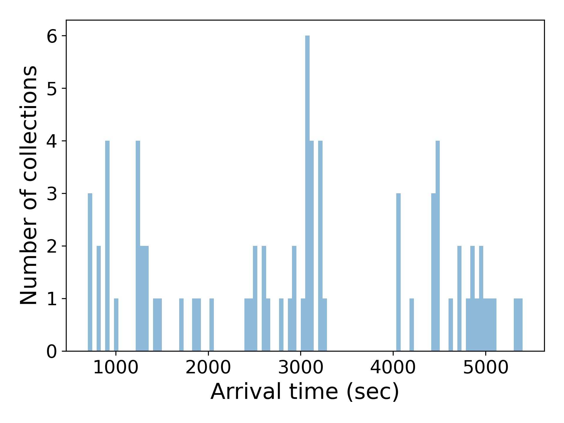
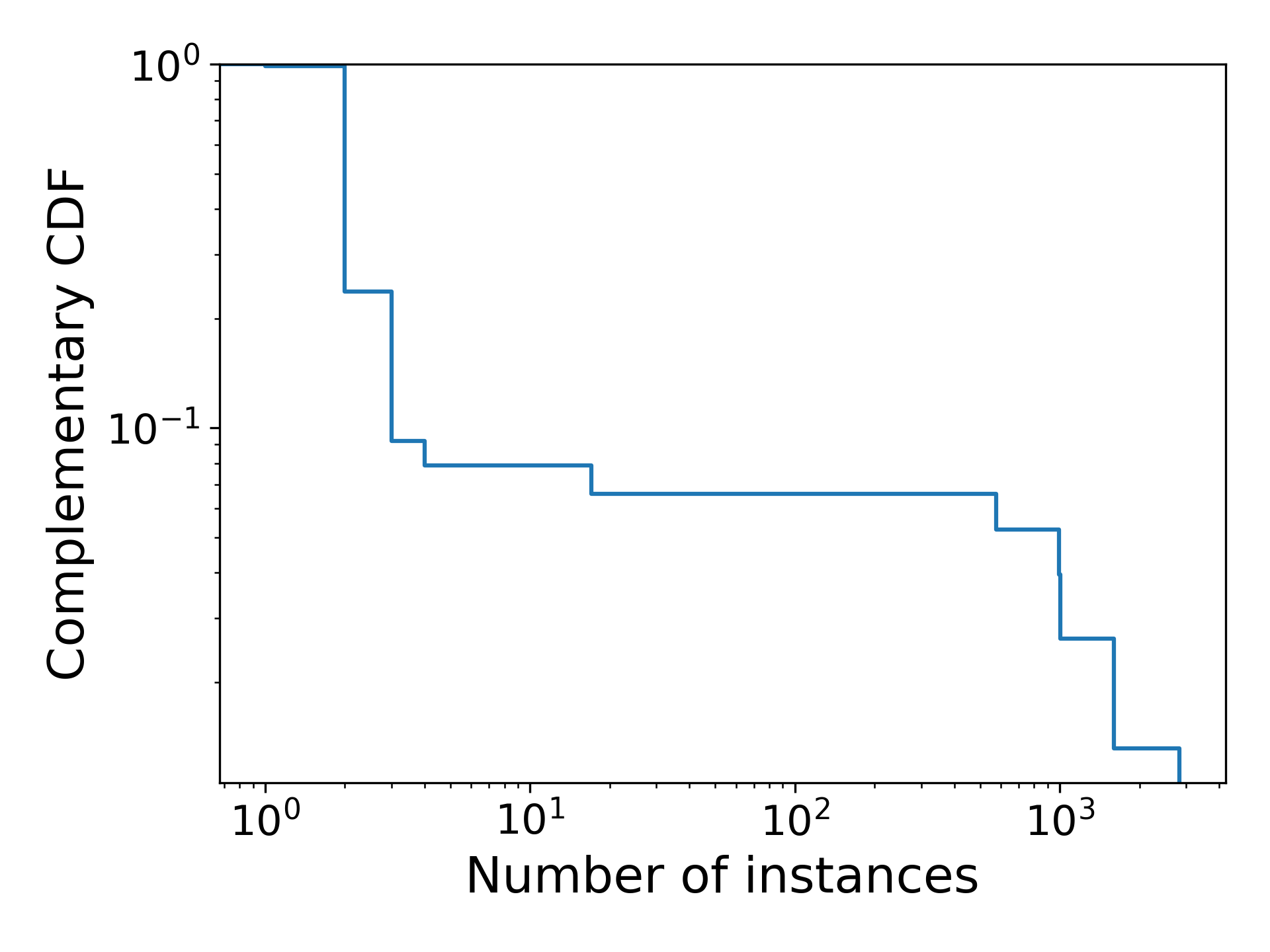
Figure 7: Characteristics of the input workload: (left) arrival of collections over time, (right) complementary cumulative distribution function of the number of instances per collection.

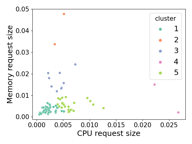
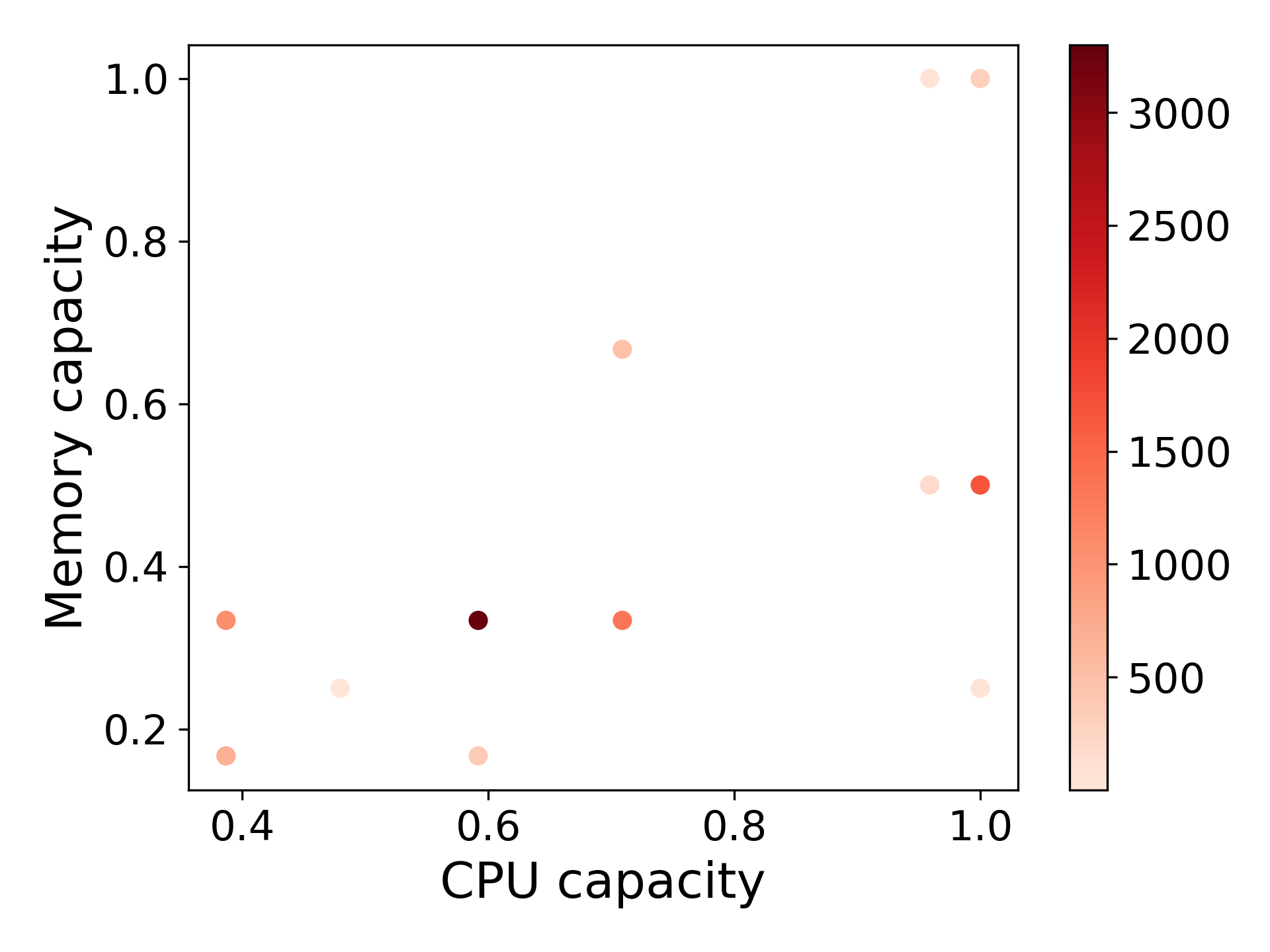
Figure 8: Feature vectors for collections and machines: (left) individual collections classified by K-means clustering with $K=5$, and (right) machine types with counts.

In this section, we provide details about the experiments using the dataset cluster-data-2019.

Basic information about the workload.

For our experiments, we used the data collected over a time interval from the beginning of the trace to 5,000 seconds of the trace. There are 9,526 machines which started before the beginning of the measurement interval and 71 enqueued collections. The arrival pattern of collections over time is shown in Figure 7 (left). The distribution of the number of instances per collection is shown in Figure 7 (right). We observe that this distribution has a heavy skew with many collections consisting of a few instances, and a small fraction of collections consisting of many instances.

Features of jobs and servers.

The dataset contains information about CPU and memory capacity of each machine and CPU and memory request size for each instance. We use this information to construct feature vectors of collections and machines. For each collection, we first represent each collection with the average CPU and the average memory request size of instances of this collection, and use this to cluster collections in 5 different classes by using the K-means clustering algorithm. These representations of collections and their clustering into classes are shown in Figure 8 (left). Each class of collections is represented by average value of CPU and memory request size of this class. For machines, we computed that there are 12 different classes of machines with respect to their CPU and memory capacities, which are shown in Figure 8 (right). In addition to CPU and memory (request) capacity values, we also used their inverse values, which amounts to using feature vectors of dimension $d=4$. This feature engineering is done in order to allow modeling inverse relationships, which is needed when using a bilinear model.

Rewards of assignments.

The dataset contains information about average number of cycles per instruction (CPI) for each assignment of an instance to a machine. The inverse CPI computed for an instance-machine pair, indicates how efficiently is the instance executed by the machine. This performance indicator depends on the characteristics of the computing that needs to be performed for given instance and characteristics of the machine. We use the inverse CPIs to define rewards of assignments. This is done by computing mean and variance of observed rewards for each combination of a collection class and a machine class, and setting the mean reward to zero for any combination of a collection class and a machine class for which no assignments are observed in the data. We use samples of rewards from a Gaussian distribution with mean and variance set to the computed values in our simulations.

Simulation setup.

We run scheduling algorithms over discrete time steps, each 5 seconds, which amounts to $T=1100$ time steps. All instances assigned to machines in a time step are assumed to be completely processed in this time step. Each machine is allowed to be assigned at most one instance in each time step. The traffic intensity of a collection class is defined as the ratio of the arrival rate of collections of this collection class and the mean number of instances per collection of this collection class. We used empirical estimate of arrival rate of collections of a collection class by using our input data. We used a median value of the number of instances per collection in our input data as an estimate of the mean number of instances per collection-this is done because a median value is robust to outliers.

Results.

In Figure 5, we show the estimated regret and mean queue lengths at different time steps from our experiments. We observe that our proposed algorithm has better performance than HXLB algorithm with respect to regret while at the same time has a comparable mean queue length. These results suggests that, in practical application scenarios, using features characterizing jobs and servers and a learning algorithm that leverages these features for estimating rewards of assignments can yield substantial performance gains.

References

- Abbasi-Yadkori et al. (2011) Abbasi-Yadkori Y, Pál D, Szepesvári C (2011) Improved algorithms for linear stochastic bandits. NIPS, volume 11, 2312–2320.
- Berthet and Baldin (2020) Berthet Q, Baldin N (2020) Statistical and computational rates in graph logistic regression. Chiappa S, Calandra R, eds., Proceedings of the Twenty Third International Conference on Artificial Intelligence and Statistics, volume 108 of Proceedings of Machine Learning Research, 2719–2730 (PMLR).
- Bramson et al. (2021) Bramson M, D’Auria B, Walton N (2021) Stability and instability of the maxweight policy. Mathematics of Operations Research 46(4):1611–1638.
- Chu and Park (2009) Chu W, Park ST (2009) Personalized recommendation on dynamic content using predictive bilinear models. 691–700, WWW ’09 (New York, NY, USA: Association for Computing Machinery).
- Georgiadis et al. (2006) Georgiadis L, Neely MJ, Tassiulas L (2006) Resource allocation and cross-layer control in wireless networks. Found. Trends Netw. 1(1):1–144.
- Gog et al. (2016) Gog I, Schwarzkopf M, Gleave A, Watson RNM, Hand S (2016) Firmament: Fast, centralized cluster scheduling at scale. 12th USENIX Symposium on Operating Systems Design and Implementation (OSDI 16), 99–115 (Savannah, GA: USENIX Association).
- Hager (1989) Hager WW (1989) Updating the inverse of a matrix. SIAM Review 31(2):221–239.
- Hsu et al. (2021) Hsu WK, Xu J, Lin X, Bell MR (2021) Integrated online learning and adaptive control in queueing systems with uncertain payoffs. Operations Research .
- Isard et al. (2009) Isard M, Prabhakaran V, Currey J, Wieder U, Talwar K, Goldberg A (2009) Quincy: Fair scheduling for distributed computing clusters. Proceedings of the ACM SIGOPS 22nd Symposium on Operating Systems Principles, 261–276, SOSP ’09 (New York, NY, USA: Association for Computing Machinery).
- Jang et al. (2021) Jang K, Jun KS, Yun SY, Kang W (2021) Improved regret bounds of bilinear bandits using action space analysis. Meila M, Zhang T, eds., Proceedings of the 38th International Conference on Machine Learning, volume 139 of Proceedings of Machine Learning Research, 4744–4754 (PMLR).
- Jiang and Walrand (2010) Jiang L, Walrand J (2010) Scheduling and Congestion Control for Wireless and Processing Networks (Morgan & Claypool Publishers).
- Johari et al. (2021) Johari R, Kamble V, Kanoria Y (2021) Matching while learning. Operations Research 69(2):655–681.
- Jun et al. (2019) Jun KS, Willett R, Wright S, Nowak R (2019) Bilinear bandits with low-rank structure. Chaudhuri K, Salakhutdinov R, eds., Proceedings of the 36th International Conference on Machine Learning, volume 97 of Proceedings of Machine Learning Research, 3163–3172 (PMLR).
- Kelly (1997) Kelly F (1997) Charging and rate control for elastic traffic. European Transactions on Telecommunications 8(1):33–37.
- Kelly et al. (1998) Kelly F, Maulloo AK, Tan DKH (1998) Rate control for communication networks: shadow prices, proportional fairness and stability. Journal of the Operational Research Society 49:237–252.
- Kelly and Voice (2005) Kelly F, Voice T (2005) Stability of end-to-end algorithms for joint routing and rate control. ACM SIGCOMM Computer Communication Review 35(2):5–12.
- Kelly and Yudovina (2014) Kelly F, Yudovina E (2014) Stochastic Networks. Institute of Mathematical Statistics Textbooks (Cambridge University Press).
- Krishnasamy et al. (2018) Krishnasamy S, Arapostathis A, Johari R, Shakkottai S (2018) On learning the c rule: Single and multiserver settings. CoRR abs/1802.06723.
- Krishnasamy et al. (2021) Krishnasamy S, Sen R, Johari R, Shakkottai S (2021) Learning unknown service rates in queues: A multiarmed bandit approach. Operations Research 69(1):315–330.
- Lattimore and Szepesvári (2020) Lattimore T, Szepesvári C (2020) Bandit Algorithms (Cambridge University Press).
- Levi et al. (2019) Levi R, Magnanti T, Shaposhnik Y (2019) Scheduling with testing. Management Science 65(2):776–793.
- Mandelbaum and Stolyar (2004) Mandelbaum A, Stolyar AL (2004) Scheduling flexible servers with convex delay costs: Heavy-traffic optimality of the generalized c-rule. Operations Research 52(6):836–855.
- Massoulié (2007) Massoulié L (2007) Structural properties of proportional fairness: Stability and insensitivity. The Annals of Applied Probability 17(3):809 – 839.
- Massoulié and Xu (2018) Massoulié L, Xu K (2018) On the capacity of information processing systems. Operations Research 66(2):568–586.
- McKeown et al. (1999) McKeown N, Mekkittikul A, Anantharam V, Walrand J (1999) Achieving 100% throughput in an input-queued switch. IEEE Transactions on Communications 47(8):1260–1267.
- Meyer (2000) Meyer CD (2000) Matrix analysis and applied linear algebra (SIAM).
- Mo and Walrand (2000) Mo J, Walrand J (2000) Fair end-to-end window-based congestion control. IEEE/ACM Transactions on Networking 8(5):556–567.
- Nazari and Stolyar (2019a) Nazari M, Stolyar AL (2019a) Reward maximization in general dynamic matching systems. Queueing Systems 91(1):143–170.
- Nazari and Stolyar (2019b) Nazari M, Stolyar AL (2019b) Reward maximization in general dynamic matching systems. Queueing Systems 91:143–170.
- Neely (2010) Neely MJ (2010) Stochastic Network Optimization with Application to Communication and Queueing Systems (Morgan&Claypool Publishers).
- Nickel et al. (2016) Nickel M, Murphy K, Tresp V, Gabrilovich E (2016) A review of relational machine learning for knowledge graphs. Proceedings of the IEEE 104(1):11–33.
- Qin et al. (2014) Qin L, Chen S, Zhu X (2014) Contextual combinatorial bandit and its application on diversified online recommendation. Proceedings of the 2014 SIAM International Conference on Data Mining, 461–469 (SIAM).
- Rizk et al. (2021) Rizk G, Thomas A, Colin I, Laraki R, Chevaleyre Y (2021) Best arm identification in graphical bilinear bandits. Meila M, Zhang T, eds., Proceedings of the 38th International Conference on Machine Learning, volume 139 of Proceedings of Machine Learning Research, 9010–9019.
- Shah et al. (2020) Shah V, Gulikers L, Massoulié L, Vojnović M (2020) Adaptive matching for expert systems with uncertain task types. Operations Research 68(5):1403–1424.
- Srikant and Ying (2013) Srikant R, Ying L (2013) Communication Networks: An Optimization, Control, and Stochastic Networks Perspective (Cambridge University Press).
- Stahlbuhk et al. (2021) Stahlbuhk T, Shrader B, Modiano E (2021) Learning algorithms for minimizing queue length regret. IEEE Transactions on Information Theory 67(3):1759–1781.
- Stolyar (2005) Stolyar AL (2005) Maximizing queueing network utility subject to stability: Greedy primal-dual algorithm. Queueing Systems 50(4):401–457.
- Talebi and Proutiere (2018) Talebi MS, Proutiere A (2018) Learning proportionally fair allocations with low regret. Proc. ACM Meas. Anal. Comput. Syst. 2(2).
- Tassiulas and Ephremides (1992) Tassiulas L, Ephremides A (1992) Stability properties of constrained queueing systems and scheduling policies for maximum throughput in multihop radio networks. IEEE Transactions on Automatic Control 37(12):1936–1948.
- Tirmazi et al. (2020) Tirmazi M, Barker A, Deng N, Haque ME, Qin ZG, Hand S, Harchol-Balter M, Wilkes J (2020) Borg: The next generation. Proceedings of the Fifteenth European Conference on Computer Systems, EuroSys ’20 (New York, NY, USA: Association for Computing Machinery).
- Verma et al. (2015) Verma A, Pedrosa L, Korupolu M, Oppenheimer D, Tune E, Wilkes J (2015) Large-scale cluster management at Google with Borg. Proceedings of the Tenth European Conference on Computer Systems, EuroSys ’15 (New York, NY, USA: Association for Computing Machinery).
- Walton (2014) Walton NS (2014) Concave switching in single and multihop networks. ACM SIGMETRICS Performance Evaluation Review 42(1):139–151.