Process Tomography on a 7-Qubit Quantum Processor
via Tensor Network Contraction Path Finding

Abstract

Quantum process tomography (QPT), where a quantum channel is reconstructed through the analysis of repeated quantum measurements, is an important tool for validating the operation of a quantum processor. We detail the combined use of an existing QPT approach based on tensor networks (TNs) and unsupervised learning with TN contraction path finding algorithms in order to use TNs of arbitrary topologies for reconstruction. Experiments were conducted on the 7-qubit IBM Quantum Falcon Processor ibmq_casablanca, where we demonstrate this technique by matching the topology of the tensor networks used for reconstruction with the topology of the processor, allowing us to extend past the characterisation of linear nearest neighbour circuits. Furthermore, we conduct single-qubit gate set tomography (GST) on each individual qubit to correct for separable errors during the state preparation and measurement phases of QPT, which are separate from the channel under consideration but may negatively impact the quality of its reconstruction. We are able to report a fidelity of 0.89 against the ideal unitary channel of a single-cycle random quantum circuit performed on ibmq_casablanca, after obtaining just $1.1\text{\times}{10}^{5}$ measurements for the reconstruction of this 7-qubit process. This represents more than five orders of magnitude fewer total measurements than the number needed to conduct full, traditional QPT on a 7-qubit process.

I Introduction

As the development of quantum computing hardware continues to progress [1, 2], there is an increasing need for scalable techniques to characterise imperfect qubit processes. The standard approach for a full characterisation of the process for a physical instance of a quantum circuit is quantum process tomography (QPT) [3, 4]. In QPT, the process for a circuit on $n$ qubits is reconstructed from a sufficiently large set of measurements made from an informationally complete set of circuit input and output settings. As such, estimating the $O(2^{4n})$-sized Choi matrix [5, 6] which uniquely describes the process on $n$ qubits through the standard QPT procedure scales exponentially in time. This prohibitive time cost has limited the use of the standard QPT procedure to general processes on up to 2 or 3 qubits [7, 8, 9, 10, 11, 12, 13].

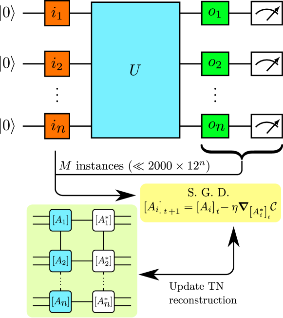
Figure 1: The general procedure for QPT of a circuit $U$ based on tensor networks with unsupervised learning [14]. Here, $M$ instances of $U$ are constructed with input states and output measurement bases drawn from an informationally complete set, configured by the choice of $i_{j}$ and $o_{j}$ rotations respectively. With single-shot measurement outcomes from each configuration, an optimisation loop based on stochastic gradient descent (SGD) with adaptive learning rate $\eta$ and cost $\mathcal{C}$ can be performed in order to update the tensors $\quantity[A_{j}]$ of a tensor network representation of the reconstructed process’ Choi matrix. For processes of sufficiently small tensor network bond and Kraus dimensions, the total number of required measurements $M$ may be significantly less than the $\mathcal{O}(12^{n})$ required for full QPT via the traditional approach.

When constrained by the limited connectivity, available basis gate operations and error rates of near-term quantum devices, only circuits with particular structure can actually be performed while maintaining a high level of coherence. The use of tensor network (TN) based algorithms [15, 16, 17] has proven extremely successful in exploiting such structure in order to reduce classical costs in problems such as quantum circuit simulation [18, 19, 20, 21], calculating Hamiltonian ground states [22] and simulating time evolution [23, 24, 25] whenever such structure permits. In these algorithms, the classical time costs [26] will typically scale as a function of entanglement induced by the circuit [27] and the error rates of the target device [2, 28, 29, 30], as opposed to just the system’s size in qubits.

Recently, the use of tensor networks has been applied to the approximate characterisation of sufficiently noiseless instances of large quantum circuits with one-dimensional topologies [14]. This TN-based approach for QPT also requires a smaller set of measurement data, which is then used to derive the final estimate of the process through an optimisation loop inspired by those typical in unsupervised learning algorithms. A schematic of the procedure is shown in Fig. 1. We also note other approaches for QPT which operate on measurement data sets with restricted size such as ansatz bootstrapping [8] and self-guided QPT [31], as well as compressed sensing [32, 33] and shadow tomography [34, 35] for quantum state tomography (QST).

In this work, we develop the tensor network QPT approach in two ways. First, by employing algorithms for finding optimal (or heuristically efficient) orderings for the pairwise contractions of tensors within a TN [36, 37], we alleviate the limitation that the original TN-based procedure had with characterising circuits not easily described in one dimension. Second, we recognise that the preparation of the states for input to the circuit and the subsequent qubit measurements made during the data collection are themselves affected by noise but not characterised by QPT as part of the circuit’s process, so we apply single-qubit corrections derived from gate set tomography [38, 39] to mitigate separable errors outside of the main process.

Finally, we present the results of experiments using our TN-based QPT on circuits run on the ibmq_casablanca quantum processor [40]. This device has 7 qubits in an I-beam topology, making it a suitable test for our approach. We were able to provide a reconstruction for a 7-qubit random quantum circuit through $1.1\text{\times}{10}^{5}$ single-shot measurement data points; significantly less than the $\approx$7\text{\times}{10}^{10}$$ measurements required when performing the full, traditional QPT on 7 qubits.

II Review of Tensor Network Based QPT with Unsupervised Learning

We review the procedure for tensor network based QPT introduced by Torlai et al. [14]. For a quantum channel on $N$ qubits described by a completely positive trace-preserving (CPTP) map $\mathcal{E}$, a reconstruction $\bm{\Lambda}_{\bm{\vartheta}}$ is generated for the corresponding Choi matrix $\bm{\Lambda}_{\mathcal{E}}$ [6]. The reconstruction $\bm{\Lambda}_{\bm{\vartheta}}$ is represented by a TN structure known as a locally purified density operator (LPDO) [41]. In this TN representation, each qubit $q_{j}$ acted on by the reconstructed process $\bm{\Lambda}_{\bm{\vartheta}}$ is associated with a tensor $\quantity[A_{j}]$ and its elementwise conjugate $\quantity[A_{j}^{*}]$. Each of the tensors $\quantity[A_{j}]$ are then connected to each other according to some topology (linear nearest neighbour (LNN) in the case of [14]), and the tensors $\quantity[A_{j}^{*}]$ are connected similarly. Finally, a Kraus bond is formed between each $\quantity[A_{j}]$ with its corresponding $\quantity[A_{j}^{*}]$. For the LNN LPDO, the elements $\matrixelement{\bm{\sigma},\bm{\tau}}{\bm{\Lambda}_{\bm{\vartheta}}}{\bm{\sigma}^{\prime},\bm{\tau}^{\prime}}$ of the Choi matrix $\bm{\Lambda}_{\bm{\vartheta}}$ with input basis $\quantity{\ket{\bm{\sigma}}}$ and output basis $\quantity{\ket{\bm{\tau}}}$ are given by the contraction of the entire LPDO:

$$\matrixelement{\bm{\sigma},\bm{\tau}}{\bm{\Lambda}_{\bm{\vartheta}}}{\bm{\sigma}^{\prime},\bm{\tau}^{\prime}}=\sum_{\quantity{\bm{\mu},\bm{\mu}^{\prime},\bm{\nu}}}\prod_{j=1}^{N}\quantity[A_{j}]_{\mu_{j-1},\nu_{j},\mu_{j}}^{\tau_{j},\sigma_{j}}\quantity[A_{j}^{*}]_{\mu_{j-1}^{\prime},\nu_{j},\mu_{j}^{\prime}}^{\tau_{j}^{\prime},\sigma_{j}^{\prime}},$$ (1)

where the Kraus bond between $\quantity[A_{j}]$ and $\quantity[A_{j}^{*}]$ is indexed by $\nu_{j}$, and the LNN bonds within the non-conjugate layer $\quantity{\quantity[A_{j}]}$ and conjugate layer $\quantity{\quantity[A_{j}^{*}]}$ are indexed by $\quantity{\mu_{j}}$ and $\quantity{\mu_{j}^{\prime}}$ respectively. Examples of these LPDO tensor networks are shown in Fig. 2.

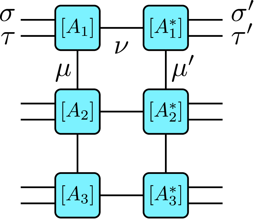
(a)

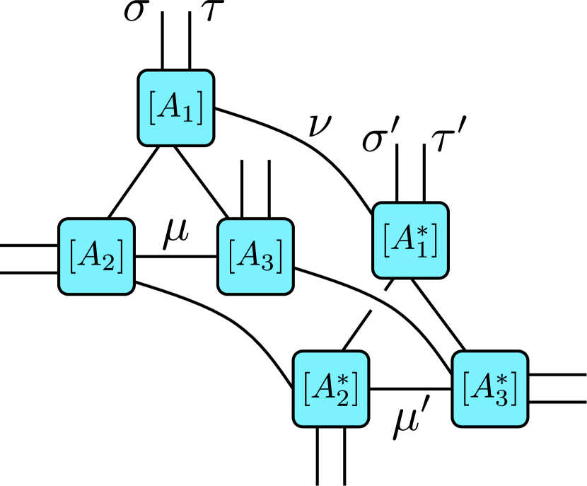
(b)

Figure 2: Example LPDO tensor networks for 3-qubit processes. In both cases, the Kraus bond indexed by $\nu_{j}$ connects tensor $\quantity[A_{j}]$ with its conjugate $\quantity[A_{j}^{*}]$, and indices $\quantity{\sigma_{j},\sigma_{j}^{\prime}}$ and $\quantity{\tau_{j},\tau_{j}^{\prime}}$ are used for inputs and outputs to the process respectively. (a) An LPDO in the linear nearest neighbour configuration used in [14], where bonds indexed by $\quantity{\mu_{j}}$ connect pairs of consecutive tensors from the non-conjugate layer $\quantity{\quantity[A_{j}]}$. (b) A fully connected configuration, where each pair of tensors within the non-conjugate layer is joined by some bond.

In order for the corresponding map of the reconstructed Choi matrix $\bm{\Lambda}_{\bm{\vartheta}}$ to be CP, $\bm{\Lambda}_{\bm{\vartheta}}$ must be positive semidefinite, which is enforced by the LPDO tensor network structure through the conjugate and non-conjugate layers. For this same map to be TP, the partial trace over the outputs of the Choi matrix should result in the identity over the inputs, so that $\Tr_{\bm{\tau}}\bm{\Lambda}_{\bm{\vartheta}}=I_{\bm{\sigma}}$. The normalisation $Z=\Tr_{\bm{\sigma},\bm{\tau}}\bm{\Lambda}_{\bm{\vartheta}}$ of the Choi matrix should be set at $d^{2N}$, where $d=2$ for qubits.

The complex-valued tensors in the non-conjugate layer $\quantity{\quantity[A_{j}]}$ form the variational parameters ${\bm{\vartheta}}$ and are iteratively trained via the following procedure. Data from the considered channel $\mathcal{E}$ is gathered by applying it to the input product state $\rho_{\bm{\alpha}}=\bigotimes_{j=1}^{N}\rho_{\alpha_{j}}$ of single-qubit states $\rho_{\alpha_{j}}$ each chosen from a set of size $K_{p}$. Following the channel, a measurement $M_{\bm{\beta}}=\bigotimes_{j=1}^{N}M_{\beta_{j}}$ is obtained by applying a positive operator-valued measure (POVM) $\quantity{M_{\beta_{j}}}_{\beta_{j}=1}^{K_{m}}$ with $K_{m}$ outcomes to each qubit. A single data point is therefore distinguished by its input tuple $\bm{\alpha}=\quantity(\alpha_{1},\ldots,\alpha_{N})$ and output tuple $\bm{\beta}=\quantity(\beta_{1},\ldots,\beta_{N})$ containing the indices of the elements within the set of input states used and within the POVM measured. The chosen set of single-qubit input states and POVM should both be informationally complete to ensure unique characterisation of $\mathcal{E}$.

The probability $P_{{\bm{\vartheta}}}\quantity(\bm{\beta}\mid\bm{\alpha})$ for the properly normalised reconstructed process $\bm{\Lambda}_{\bm{\vartheta}}$ to produce the measurements $M_{\bm{\beta}}$ given the input state $\rho_{\bm{\alpha}}$ is calculated via the tensor network contraction of

$$P_{{\bm{\vartheta}}}\quantity(\bm{\beta}\mid\bm{\alpha}) =\Tr_{\bm{\sigma},\bm{\tau}}\quantity[\quantity(\rho_{\bm{\alpha}}^{T}\otimes M_{\bm{\beta}})\bm{\Lambda}_{\bm{\vartheta}}],$$ (2)

an example of which is shown in Fig. 3. With a mini-batch of $M$ data points consisting of uniformly sampled input index tuples $\quantity{\bm{\alpha}_{k}}_{k=1}^{M}$ with their respective measurement tuples $\quantity{\bm{\beta}_{k}}_{k=1}^{M}$, some form of gradient descent may be applied to optimise for the parameters $\bm{\vartheta}$ with respect to the mean negative log-likelihood $-\frac{1}{M}\sum_{k=1}^{M}\log P_{{\bm{\vartheta}}}\quantity(\bm{\beta}_{k}\mid\bm{\alpha}_{k})$. To control convergence toward the TP condition $\Tr_{\bm{\tau}}\bm{\Lambda}_{\bm{\vartheta}}=I_{\bm{\sigma}}$, the regularisation term

$$\Gamma_{\bm{\vartheta}}=\sqrt{d^{-N}\Tr_{\bm{\sigma}}(\bm{\Delta}_{\bm{\vartheta}}\bm{\Delta}_{\bm{\vartheta}}^{\dagger})}$$ (3)

where $\bm{\Delta}_{\bm{\vartheta}}=\Tr_{\bm{\tau}}\bm{\Lambda}_{\bm{\vartheta}}-I_{\bm{\sigma}}$ is calculated through tensor network operations (see [14, Fig. 10]), giving a final cost function of

$$\mathcal{C}\quantity(\bm{\vartheta})=-\frac{1}{M}\sum_{k=1}^{M}\log P_{{\bm{\vartheta}}}\quantity(\bm{\beta}_{k}\mid\bm{\alpha}_{k})+\kappa\Gamma_{\bm{\vartheta}}$$ (4)

over the mini-batch, where $\kappa$ is a tunable hyperparameter. The appropriate Wirtinger derivatives [42] for complex-valued gradient descent may be calculated through automatic differentiation.

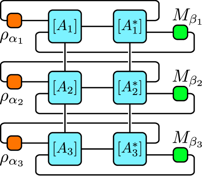
Figure 3: The tensor network expression for $P_{{\bm{\vartheta}}}\quantity(\bm{\beta}\mid\bm{\alpha})$ of an $N=3$ qubit linear nearest neighbour LPDO. This is the probability of obtaining a measurement $M_{\bm{\beta}}=\bigotimes_{j=1}^{N}M_{\beta_{j}}$ after applying the normalised reconstructed process $\bm{\Lambda}_{\bm{\vartheta}}$ to the initial state $\rho_{\bm{\alpha}}=\bigotimes_{j=1}^{N}\rho_{\alpha_{j}}$.

III Extensions to the QPT Procedure

We introduce two extensions to the original QPT procedure based on tensor networks with unsupervised learning detailed in the previous section. For our implementation, we used the JAX library [43] for GPU acceleration, automatic differentiation and automatic vectorisation, and the TensorNetwork library [44] for tensor network semantics.

III.1 LPDOs with Arbitrary Topologies

The numerical experiments presented in [14] were performed using LPDO tensor networks with 1-dimensional linear nearest neighbour (LNN) connectivity. These networks allow for an optimal contraction strategy for calculating derivatives and performing simulated QPT measurement sampling. However, they are not well suited for characterising processes on quantum systems without 1D LNN connectivity since any non-LNN interaction may result in an increase in the dimension of all bonds spanned by the interaction.

As such, we introduce the use of LPDOs with arbitrary topologies (which still follow the structure of an LPDO, with a conjugate and non-conjugate layer connected with a Kraus bond per site), an example of which is provided in Fig. LABEL:sub@fig:arb_lpdo. These tensor networks do not have a single strategy for performing optimised contractions, unlike the 1D LNN LPDOs. Instead, algorithms such as those implemented in the opt_einsum library [45] for finding contraction orderings with optimised floating point operations count were used [36]. We combine the use of these algorithms for finding contraction orderings with automatic vectorisation from JAX to ensure that efficient contractions of an entire mini-batch’s worth of probabilities $\quantity{P_{{\bm{\vartheta}}}\quantity(\bm{\beta}_{k}\mid\bm{\alpha}_{k})}$ could be performed. Finally, automatic differentiation [46] is applied in order to calculate gradients for the purpose of optimisation.

III.2 Gate Set Tomography

When gathering data points on a physical device, errors introduced during input state initialisation and final POVM measurement will result in a different actual input state and POVM than those specified during the classical reconstruction. As such, we perform single-qubit gate set tomography (GST) [38, 39] on each qubit to obtain its input state set and POVM corrected for single-qubit errors. These input state sets and POVMs specific for each qubit were then used in the relevant tensor network contractions, such as in the calculation of $P_{{\bm{\vartheta}}}\quantity(\bm{\beta}\mid\bm{\alpha})$. We performed GST using the pyGSTi library [47].

IV Results

We present results for QPT experiments performed on the ibmq_casablanca 7-qubit system, one of the IBM Falcon Quantum Processors, whose I-beam topology shown in Fig. 4 we match with the LPDO tensor network. Unless otherwise noted, we use a regularisation weight $\kappa=0.1$ and the Adam optimiser [48] with default parameters. We perform each experiment and gather the corresponding GST corrections in a contiguous reserved time slot in order to minimise the potential for large calibration changes in the device itself. The $\sqrt{X}$ and CNOT error rates averaged over this time slot are also shown in Fig. 4.

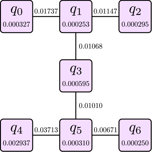
Figure 4: The I-beam topology of the ibmq_casablanca quantum computer of the 7 superconducting qubits labelled $q_{0}$ to $q_{6}$. The values inside each node is the $\sqrt{X}$ error rate for that qubit as recorded in the device’s calibration data, averaged over the measurement data collection period. Similarly, the edge values are the time-averaged reported error rates for a CNOT gate applied in either direction between the two associated qubits. During our reconstructions, the topology of the LPDOs used was matched to this configuration.

For each of our experiments, we use the informationally complete set of single-qubit states containing

$$X_{+} =\outerproduct{+}{+}, X_{-} =\outerproduct{-}{-},$$

$$Y_{+} =\outerproduct{+i}{+i}, Y_{-} =\outerproduct{-i}{-i},$$

$$Z_{+} =\outerproduct{0}{0}, Z_{-} =\outerproduct{1}{1}$$

to select inputs $\rho_{\alpha_{j}}$ to the channel for each data instance. We use the same set properly normalised (i.e. $\quantity{X_{\pm}/3,Y_{\pm}/3,Z_{\pm}/3}$) as the single-qubit POVM $M_{\beta_{j}}$ for each qubit following the channel. The chosen inputs $\rho_{\alpha_{j}}$ are prepared by performing the relevant single-qubit rotation from the default initial state $\ket{0}$, and the POVM measurements are emulated by choosing either the $X$, $Y$ or $Z$ basis uniformly at random to measure in (which consists of performing the necessary rotation and final computational basis measurement). We performed separate instances of GST on each qubit in parallel to better characterise the actual input states $\rho_{\alpha_{j}}$ and output POVMs $M_{\beta_{j}}$ used in our experiments. These corrections were then used during the numerical reconstruction procedure. We place barriers in between the state initialisation, process and final measurement to prevent compiler optimisation across these phases.

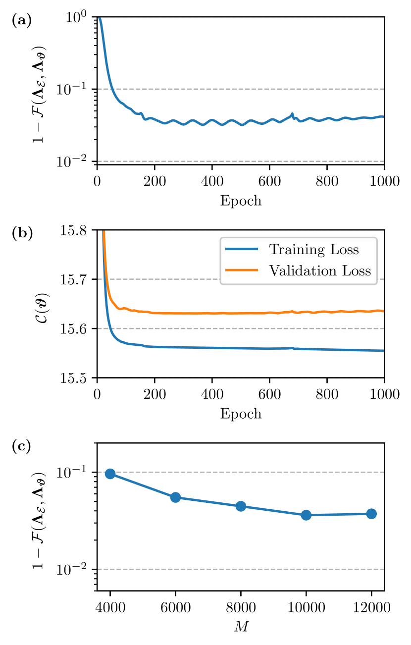
Figure 5: QPT results of the single Hadamard layer on ibmq_casablanca. The tensor network for the reconstruction $\bm{\Lambda}_{\bm{\vartheta}}$ was set with all bond and Kraus dimensions of size 5. (a) The infidelity of the reconstruction $\bm{\Lambda}_{\bm{\vartheta}}$ with $M=$1.2\text{\times}{10}^{4}$$ against the ideal unitary Hadamard layer process $\bm{\Lambda}_{\mathcal{E}}$ and (b) the loss over the training data set of size $M=$1.2\text{\times}{10}^{4}$$ and the validation data set of size $0.25M$ at each epoch. No mini-batching was performed since the training set here was sufficiently small. The fidelity reported at the lowest validation loss was $0.963$. (c) The infidelity calculated at the point of lowest validation loss over 1000 training epochs with various data set sizes $M$, where the validation data set has size $0.25M$ in each instance.

Our first experiment involved characterising the process of a single layer of Hadamard gates performed on ibmq_casablanca. In Fig. 5(a), we show the fidelity $\mathcal{F}\quantity(\bm{\Lambda}_{\mathcal{E}},\bm{\Lambda}_{\bm{\vartheta}})$ between our reconstruction $\bm{\Lambda}_{\bm{\vartheta}}$ against the ideal unitary Hadamard layer process $\bm{\Lambda}_{\mathcal{E}}$. Typically, this is calculated as

$$\mathcal{F}\quantity(\bm{\Lambda}_{\mathcal{E}},\bm{\Lambda}_{\bm{\vartheta}}) =d^{-2N}\quantity(\Tr\sqrt{\sqrt{\bm{\Lambda}_{\mathcal{E}}}\bm{\Lambda}_{\bm{\vartheta}}\sqrt{\bm{\Lambda}_{\mathcal{E}}}})^{2}$$ (5)

when $\bm{\Lambda}_{\mathcal{E}}$ and $\bm{\Lambda}_{\bm{\vartheta}}$ are properly normalised. In the general case this calculation is not efficient, but when $\bm{\Lambda}_{\mathcal{E}}$ is a unitary process such as our Hadamard layer, its LPDO tensor network will have trivial Kraus bonds of dimension 1, essentially disconnecting the non-conjugate and conjugate layers (which we denote as $\ket{\bm{\Lambda}_{\mathcal{E}}}$ and $\bra{\bm{\Lambda}_{\mathcal{E}}}$ respectively, so that $\bm{\Lambda}_{\mathcal{E}}=\outerproduct{\bm{\Lambda}_{\mathcal{E}}}{\bm{\Lambda}_{\mathcal{E}}}$). In this case, the fidelity calculation reduces to the efficient tensor network contraction $\mathcal{F}\quantity(\bm{\Lambda}_{\mathcal{E}},\bm{\Lambda}_{\bm{\vartheta}})=d^{-2N}\expectationvalue{\bm{\Lambda}_{\bm{\vartheta}}}{\bm{\Lambda}_{\mathcal{E}}}$.

In Fig. 5(b), we present the loss $\mathcal{C}\quantity(\bm{\vartheta})$ over the training data set of size $M=$1.2\text{\times}{10}^{4}$$ over the duration of the training period. To prevent overfitting when selecting the most appropriate model parameters $\bm{\vartheta}_{t}$ at some epoch $t$, we perform cross-validation by calculating the loss over a distinct validation set of size $0.25M$ at each epoch. We then select the parameters $\bm{\vartheta}_{t}$ which result in the lowest validation loss across all training epochs. With these parameters, our reconstruction suggests that ibmq_casablanca performed the 7-qubit Hadamard layer with a fidelity of $0.963$. Furthermore, in Fig. 5(c), we show the infidelity with respect to training set size $M$. Convergence here suggests that a sufficiently large training set was indeed used to derive an accurate reconstruction.

Upon transpilation of the 7-qubit Hadamard layer to the basis gate set of ibmq_casablanca, the resulting circuit contains one $\sqrt{X}$ gate on each qubit. By compounding individual $\sqrt{X}$ gate errors $r_{g}$ from the rates shown in Fig. 4, we derive a baseline fidelity $\mathcal{F}_{\text{base}}=\prod_{g}\quantity(1-r_{g})=0.995$ for the 7-qubit Hadamard layer. The presence of crosstalk and other multi-qubit errors are not captured by this value, so our reconstruction’s fidelity of $0.963$ still appears reasonable.

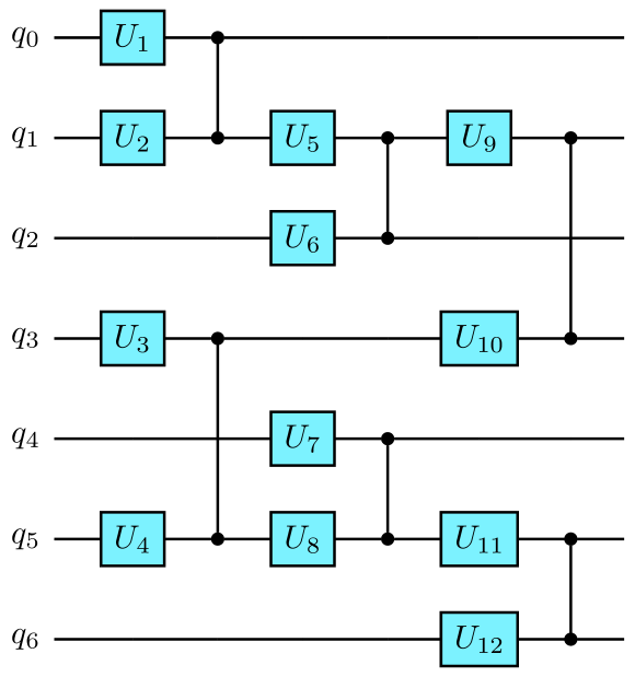
Figure 6: Circuit diagram for the random quantum circuit (RQC) characterised on ibmq_casablanca. Each of the single-qubit rotations $U_{i}$ performed before a CZ gate was randomly generated [49]. An RQC instance parameterised by the gates $\quantity{U_{i}}$ can then be characterised through QPT. Upon transpilation to the basis gate set of ibmq_casablanca, there are notably $\quantity(2,6,3,5,2,6,3)$ $\sqrt{X}$ gates on each of the qubits $q_{0}$ to $q_{6}$ and one CNOT on each edge.

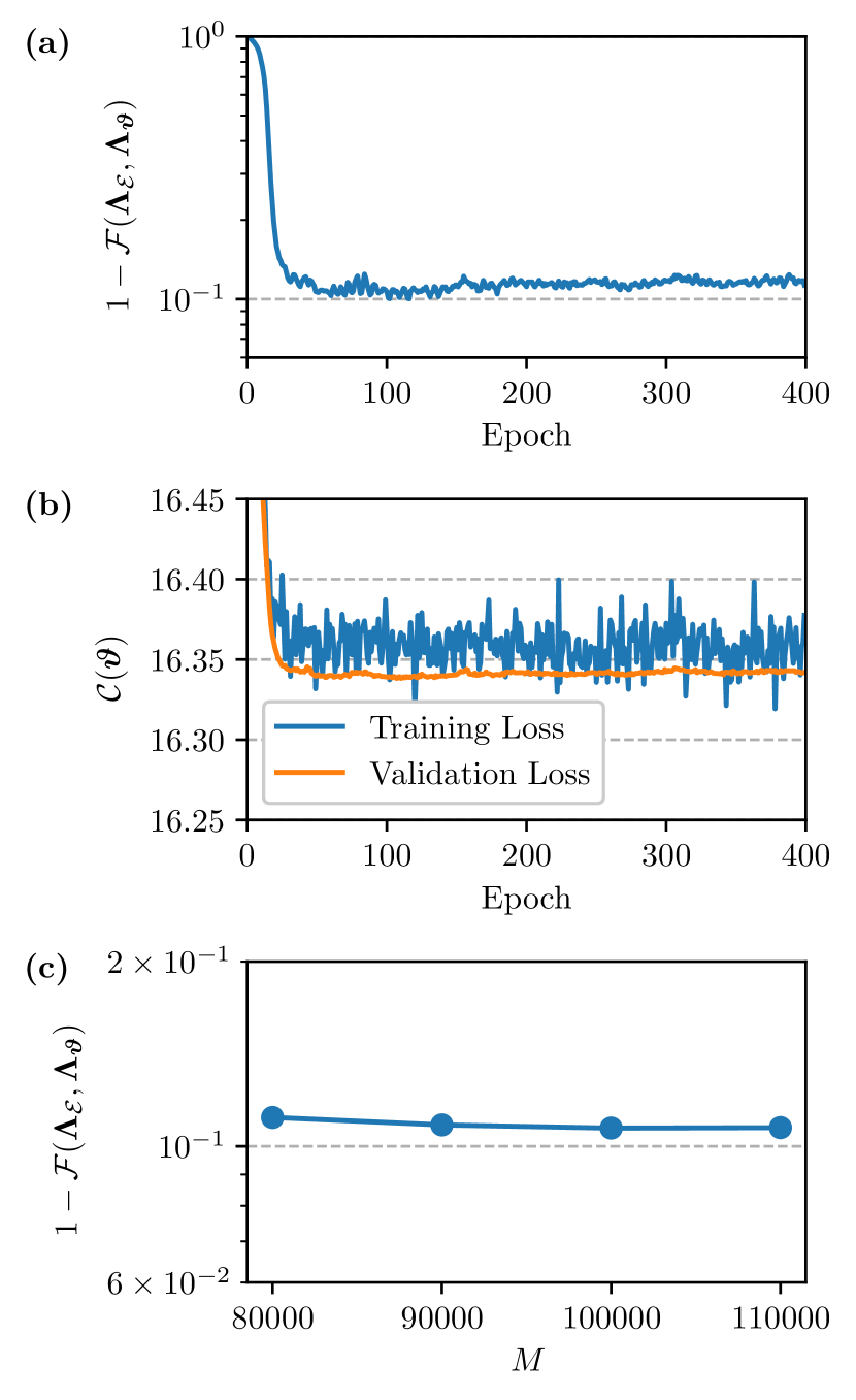
Figure 7: QPT results of the single-cycle random quantum circuit on ibmq_casablanca, where the tensor network for the reconstruction $\bm{\Lambda}_{\bm{\vartheta}}$ was set with all bond and Kraus dimensions of size 5. (a) The infidelity of the reconstruction $\bm{\Lambda}_{\bm{\vartheta}}$ against our ideal unitary single-cycle RQC process $\bm{\Lambda}_{\mathcal{E}}$ during training with $M=$1.1\text{\times}{10}^{5}$$ and (b) the loss over the training data set of size $M=$1.1\text{\times}{10}^{5}$$ and the validation data set of size $0.25M$ at each epoch. Mini-batches of size $1\text{\times}{10}^{4}$ were used. The fidelity reported at the lowest validation loss was $0.892$. (c) The infidelity calculated at the point of lowest validation loss over 400 training epochs with various data set sizes $M$, where the validation data set has size $0.25M$ in each instance.

Next, we performed experiments to characterise single-cycle random quantum circuits (RQCs) [2] with CZ gates as interactions. In these circuits, the 2-qubit interactions are applied two at a time, to pairs of qubits

1. $\quantity(q_{0},q_{1})$ and $\quantity(q_{3},q_{5})$

2. $\quantity(q_{1},q_{2})$ and $\quantity(q_{4},q_{5})$

3. $\quantity(q_{1},q_{3})$ and $\quantity(q_{5},q_{6})$.

Just before each interaction, a randomly selected single-qubit rotation [49] was applied to each of the qubits being interacted, as seen in Fig. 6. We present results for the QPT procedure in Fig. 7 for a single instance of chosen random unitaries. An ideal realisation of the single-cycle RQC with CZ interactions would be perfectly characterisable by the topologically matching LPDO with bond dimension 2 (equal to the operator Schmidt rank of the CZ gate) and Kraus dimension 1 (due to unitarity). With our reconstruction of all bond and Kraus dimensions set to 5, we report a fidelity of $0.892$ against the ideal unitary RQC process at the lowest validation loss. It is worth noting that this reconstruction was performed with just $M=$1.1\text{\times}{10}^{5}$$ data instances, each itself a single-shot measurement performed on ibmq_casablanca. By compounding the error rates in Fig. 4 with the relevant CNOT and $\sqrt{X}$ gate counts in Fig. 6, the fidelity derived from ibmq_casablanca’s own calibration data is extremely close with $\mathcal{F}_{\text{base}}=0.897$. Convergence of the reconstruction’s fidelity against the ideal unitary process shown in Fig. 7(c) again suggests that this choice of $M$ is sufficient.

Finally, we compare the reduction of the reconstruction obtained from our TN-based approach with that of the traditional, full QPT approach on the subset of qubits $\quantity{q_{1},q_{3},q_{5}}$. Here, the process on $\quantity{q_{1},q_{3},q_{5}}$ is the same single-cycle RQC over all seven qubits, but where the remaining qubits $\quantity{q_{0},q_{2},q_{4},q_{6}}$ are each initialised to $Z_{+}$. Importantly, this process is not a unitary operation on qubits $\quantity{q_{1},q_{3},q_{5}}$.

Using the default settings in Qiskit [50] for performing traditional QPT on IBM quantum systems, we use the informationally complete set of input qubit states $\quantity{Z_{+},Z_{-},X_{+},Y_{+}}$ (instead of the six possible input states used during the TN-based experiments) and measure along an axis chosen uniformly randomly from $\quantity{X,Y,Z}$ (resulting in an identical POVM set used in the TN-based experiments). Therefore, for this three-qubit process we need to perform sufficiently many measurements to obtain $12^{3}$ probability distributions. Using a typical 2000 shots per selection of input states and measurement axes gives a total of $12^{3}\times 2000=$3.46\text{\times}{10}^{6}$$ individual measurements that we performed in order to derive a reconstruction through the traditional QPT approach. We report a fidelity of 0.80 between the reconstruction derived from the traditional, full QPT approach with the ideal (non-unitary) process on the three qubits.

For the TN-based approach, we again perform tomography of the RQC across all seven qubits, but then reduce it to the three-qubit process by applying the tensor network of the reconstruction $\bm{\Lambda}_{\bm{\vartheta}}$ to the GST-corrected input states corresponding to $Z_{+}$ for qubits $\quantity{q_{0},q_{2},q_{4},q_{6}}$ and tracing the output indices associated with these qubits. An example of reducing an LPDO down to a subset of qubits is shown in Fig. 8. Using $4\text{\times}{10}^{5}$ single-shot measurements, we report a fidelity of 0.96 between the reconstruction derived from the TN-based approach against the ideal process, and a fidelity of 0.81 between the reconstructions of the TN-based and traditional approaches.

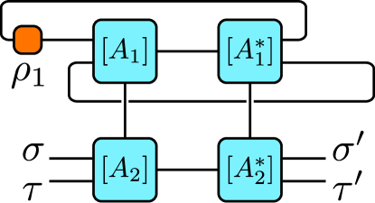
Figure 8: By performing a contraction of this tensor network, an LPDO for some process on two qubits $q_{1}$ and $q_{2}$ may be reduced to the Choi matrix for the process acting on qubit $q_{2}$, where $q_{1}$ is specifically initialised to the state $\rho_{1}$.

While the agreement between the two approaches is decent, we justify the discrepancy by noting that the traditional QPT performed through Qiskit does not include any form of GST correction, whereas our TN-based approach makes use of it to correct for single-qubit errors in the initialisation of all qubits, including qubits $\quantity{q_{0},q_{2},q_{4},q_{6}}$, and the POVM measurements. Furthermore, despite using an order of magnitude fewer total measurements, the total time taken to collect the single-shot measurements for the TN-based approach was significantly longer than the time taken to perform all measurements for the traditional approach. It is possible that changes in the device’s calibration during this prolonged data collection period may have contributed to this discrepancy between the reconstructions from each approach. This particular issue is due to shortcomings of the classical queueing and processing of circuit requests on the IBM Quantum systems which we hope can be rectified in a future update [51].

V Conclusion

We presented several extensions to an existing scheme for quantum process tomography based on tensor networks and unsupervised learning. Namely, we combined the use of algorithms for finding good tensor network contraction orderings with the typical machine learning procedures of batching and automatic differentiation to construct tensor networks with topologies matched toward a particular device architecture. This can allow for a more efficient tensor network representation of the reconstructed process when compared to the equivalent 1D tensor network of identical bond and Kraus dimensions. We also suggest the use of gate set tomography during the collection of data points in order to correct for single-qubit initialisation and measurement errors.

Experiments were conducted on the ibmq_casablanca 7-qubit quantum processor to demonstrate the use of our QPT procedure with tensor networks matched to the device’s I-beam topology. For the single Hadamard layer, we report a fidelity of $0.963$ against the ideal unitary determined from $M=$1.2\text{\times}{10}^{4}$$ single-shot measurements, and similarly a fidelity of $0.892$ for the random quantum circuit of one cycle determined from $M=$1.1\text{\times}{10}^{5}$$ measurements. Both of these measurement data sets are significantly smaller than the $2000\times 12^{7}\approx$7.2\text{\times}{10}^{10}$$ measurements needed for performing full QPT on a 7-qubit process via the traditional approach.

We then compared the reconstruction of the single-cycle RQC on ibmq_casablanca reduced to a 3-qubit subset with that of the traditional QPT procedure performed on these three qubits, and report a fidelity of $0.81$ between the reconstructions of these two approaches. Given that our TN-based approach for characterising this RQC on seven qubits used roughly an order of magnitude fewer total measurements than the traditional approach even on just three qubits, we can be confident in the viability of our approach for the characterisation of large quantum processes which can be represented as local purified density operators with manageable bond dimensions.