A Self-supervised Mixed-curvature Graph Neural Network

Abstract

Graph representation learning received increasing attentions in recent years. Most of the existing methods ignore the complexity of the graph structures and restrict graphs in a single constant-curvature representation space, which is only suitable to particular kinds of graph structure indeed. Additionally, these methods follow the supervised or semi-supervised learning paradigm, and thereby notably limit their deployment on the unlabeled graphs in real applications. To address these aforementioned limitations, we take the first attempt to study the self-supervised graph representation learning in the mixed-curvature spaces. In this paper, we present a novel Self-supervised Mixed-curvature Graph Neural Network (SelfMGNN). To capture the complex graph structures, we construct a mixed-curvature space via the Cartesian product of multiple Riemannian component spaces, and design hierarchical attention mechanisms for learning and fusing graph representations across these component spaces. To enable the self-supervisd learning, we propose a novel dual contrastive approach. The constructed mixed-curvature space actually provides multiple Riemannian views for the contrastive learning. We introduce a Riemannian projector to reveal these views, and utilize a well-designed Riemannian discriminator for the single-view and cross-view contrastive learning within and across the Riemannian views. Finally, extensive experiments show that SelfMGNN captures the complex graph structures and outperforms state-of-the-art baselines.

Introduction

Graph representation learning (Cui et al. 2018; Hamilton, Ying, and Leskovec 2017) shows fundamental importance in various applications, such as link prediction and node classification (Kipf and Welling 2017), and thus receives increasing attentions from both academics and industries. Meanwhile, we have also observed great limitations with the existing graph representation learning methods in two major perspectives, which are described as follows:

Representation Space: Most of existing methods ignore the complexity of real graph structures, and limit the graphs in a single constant-curvature representation space (Gu et al. 2019). Such methods can only work well on particular kinds of structure that they are designed for. For instance, the constant negative curvature hyperbolic space is well-suited for graphs with hierarchical or tree-like structures (Liu, Nickel, and Kiela 2019). The constant positive curvature spherical space is especially suitable for data with cyclical structures, e.g., triangles and cliques (Bachmann, Bécigneul, and Ganea 2020), and the zero-curvature Euclidean space for grid data (Wu et al. 2021). However, graph structures in reality are usually mixed and complicated rather than uniformed, in some regions hierarchical, while in others cyclical (Papadopoulos et al. 2012; Ravasz and Barabási 2003). Even more challenging, the curvatures over different hierarchical or cyclical regions can be different as will be shown in this paper. In fact, it calls for a new representation space to match the wide variety of graph structures, and we seek spaces of mixed-curvature to provide better representations.

Learning Paradigm: Learning graph representations usually requires abundant supervision label information (Veličković et al. 2018; Chami et al. 2019). Labels are usually scarce in real applications, and undoubtedly, labeling graphs is expensive—manual annotation or paying for permission, and is even impossible to acquire because of the privacy policy. Fortunately, the rich information in graphs provides the potential for self-supervised learning, i.e., learning representations without labels (Liu et al. 2021). Self-supervised graph representation learning is a more favorable choice, particularly when we intend to take the advantages from the unlabeled graphs in real applications. Recently, contrastive learning (Veličković et al. 2019; Qiu et al. 2020) emerges as a successful method for the graph self-supervised learning. However, existing self-supervised methods, to the best of our knowledge, cannot be applied to the mixed-curvature spaces due to the intrinsic differences in the geometry.

To address these aforementioned limitations, we take the first attempt to study the self-supervised graph representation learning in the mixed-curvature space in this paper.

To this end, we present a novel Self-supervised Mixed-curvature Graph Neural Network, named SelfMGNN. To address the first limitation, we propose to learn the representations in a mixed-curvature space. Concretely, we first construct a mixed-curvature space via the Cartesian product of multiple Riemannian—hyperbolic, spherical and Euclidean—component spaces, jointly enjoying the strength of different curvatures to match the complicated graph structures. Then, we introduce hierarchical attention mechanisms for learning and fusing representations in the product space. In particular, we design an intra-component attention for the learning within a component space and an inter-component attention for the fusing across component spaces. To address the second limitation, we propose a novel dual contrastive approach to enable the self-supervisd learning. The constructed mixed-curvature space actually provides multiple Riemannian views for contrastive learning. Concretely, we first introduce a Riemannian projector to reveal these views, i.e., hyperbolic, spherical and Euclidean views. Then, we introduce the single-view and cross-view contrastive learning. In particular, we utilize a well-designed Riemannian discriminator to contrast positive and negative samples in the same Riemannian view (i.e., the single-view contrastive learning) and concurrently contrast between different Riemannian views (i.e., the cross-view contrastive learning). In the experiments, we study the curvatures of real graphs and show the advantages of allowing multiple positive and negative curvature components for the first time, demonstrating the superiority of SelfMGNN.

Overall, our main contributions are summarized below:

• Problem: To the best of our knowledge, this is the first attempt to study the self-supervised graph representation learning in the mixed-curvature space.

• Model: This paper presents a novel SelfMGNN model, where hierarchical attention mechanisms and dual contrastive approach are designed for self-supervised learning in the mixed-curvature space, allowing multiple hyperbolic (spherical) components with distinct curvatures.

• Experiments: Extensive experiments show the curvatures over different hierarchical (spherical) regions of a graph can be different. SelfMGNN captures the complicated graph structures without labels and outperforms the state-of-the-art baselines.

Preliminaries and Problem Definition

In this section, we first present the preliminaries and notations necessary to construct a mixed-curvature space. Then, we formulate the problem of self-supervised graph representation learning in the mixed-curvature space.

Riemannian Manifold

A smooth manifold $\mathcal{M}$ generalizes the notion of the surface to higher dimensions. Each point $\mathbf{x}\in\mathcal{M}$ associates with a tangent space $\mathcal{T}_{\mathbf{x}}\mathcal{M}$, the first order approximation of $\mathcal{M}$ around $\mathbf{x}$, which is locally Euclidean. On tangent space $\mathcal{T}_{\mathbf{x}}\mathcal{M}$, the Riemannian metric, $g_{\mathbf{x}}(\cdot,\cdot):\mathcal{T}_{\mathbf{x}}\mathcal{M}\times\mathcal{T}_{\mathbf{x}}\mathcal{M}\to\mathbb{R}$, defines an inner product so that geometric notions can be induced. The tuple $(\mathcal{M},g)$ is called a Riemannian manifold.

Transforming between the tangent space and the manifold is done via exponential and logarithmic maps, respectively. For $\mathbf{x}\in\mathcal{M}$, the exponential map at $\mathbf{x}$, $\mathbf{exp}_{\mathbf{x}}(\mathbf{v}):\mathcal{T}_{\mathbf{x}}\mathcal{M}\to\mathcal{M}$, projects the vector $\mathbf{v}\in\mathcal{T}_{\mathbf{x}}\mathcal{M}$ onto the manifold $\mathcal{M}$. The logarithmic map at $\mathbf{x}$, $\mathbf{log}_{\mathbf{x}}(\mathbf{y}):\mathcal{M}\to\mathcal{T}_{\mathbf{x}}\mathcal{M}$, projects the vector $\mathbf{y}\in\mathcal{M}$ back to the tangent space $\mathcal{T}_{\mathbf{x}}\mathcal{M}$. For further expositions, please refer to mathematical materials (Spivak 1979; Hopper and Andrews 2010).

Constant Curvature Space

The Riemannian metric also defines a curvature at each point $\kappa(\mathbf{x})$, which determines how the space is curved. If the curvature is uniformly distributed, $(\mathcal{M},g)$ is called a constant curvature space of curvature $\kappa$. There are $3$ canonical types of constant curvature space that we can define with respect to the sign of the curvature: a positively curved spherical space $\mathbb{S}$ with $\kappa>0$, a negatively curved hyperbolic space $\mathbb{H}$ with $\kappa<0$ and the flat Euclidean space $\mathbb{E}$ with $\kappa=0$.

Note that, $\|\cdot\|_{2}$ denotes the Euclidean norm in this paper.

Problem Definition

In this paper, we propose to study the self-supervised graph representation learning in the mixed-curvature space. Without loss of generality, a graph is described as $G=(V,E,\mathbf{X})$, where $V=\{v_{1},\cdots,v_{n}\}$ is the node set and $E=\{(v_{i},v_{j})|\ v_{i},v_{j}\in V\}$ is the edge set. We summarize the edges in the adjacency matrix $\mathbf{G}$, where $\mathbf{G}_{ij}=1$ iff $(v_{i},v_{j})\in E$, otherwise $0$. Each node $v_{i}$ is associated with a feature vector $\mathbf{x}_{i}\in\mathbb{R}^{d}$, and matrix $\mathbf{X}\in\mathbb{R}^{|V|\times d}$ represents the features of all nodes. Now, we give the studied problem:

Problem Definition (Self-supervised graph representation learning in the mixed-curvature space).

Given a graph $G=(V,E,\mathbf{X})$, the problem of self-supervised graph representation learning in the mixed-curvature space is to learn an encoding function $\Phi:V\to\mathcal{P}$ that maps the node $v$ to a vector $\bm{z}$ in a mixed-curvature space $\mathcal{P}$ that captures the intrinsic complexity of graph structure without using any label information.

In other words, the graph representation model should align with the complex graph structures — hierarchical as well as cyclical structure, and can be learned without external guidance (labels). Graphs in reality are usually mixed-curvatured rather than structured uniformly, i.e., in some regions hierarchical, while in others cyclical. A constant-curvature model (e.g., hyperbolic, spherical or the Euclidean model) benefits from their specific bias to better fit particular structure types. To bridge this gap, we propose to work with the mixed-curvature space to cover the complex graph structures in real-world applications.

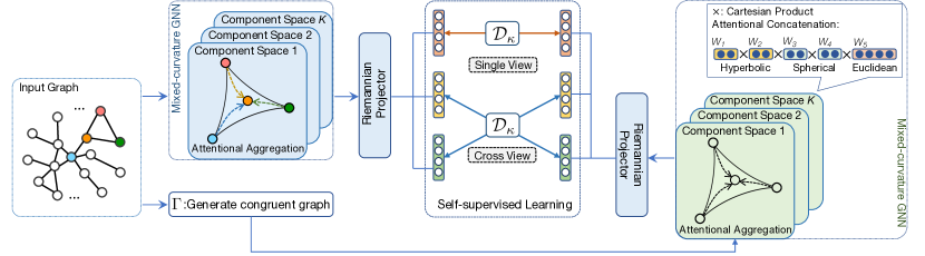
Figure 1: Overall architecture of SelfMGNN: In SelfMGNN, we first introduce a mixed-curvature GNN to learn graph representations. Specifically, we perform attentional aggregation within the component space where the triangle is to show its geometry, e.g., triangles curve inside in $\mathbb{H}$, and attentional concatenation among component spaces whose example with learnable weights is on the top right. Then, to enable self-supervised learning, we design a Riemannian projector to reveal different views of the mixed-curvature space, and utilize a well-designed Riemannian discriminator $\mathcal{D}_{\kappa}$ to contrast samples for single- and cross-view contrastive learning, shown in the middle. In practice, we feed the graph and its congruent augmentation, generated by $\Gamma(\cdot)$, for the contrastive learning as specified in Algo. 1.

SelfMGNN: Our Proposed Model

To address this problem, we present a novel Self-supervised Mixed-curvature Graph Neural Network (SelfMGNN). In a nutshell, SelfMGNN learns graph representations in the mixed-curvature space, and is equipped with a dual contrastive approach to enable its self-supervised learning. We illustrate the architecture of SelfMGNN in Fig. 1. We will elaborate on the mixed-curvature graph representation learning and the dual contrastive approach in following sections.

Mixed-curvature GNN

To learn the graph representations in a mixed-curvature space, we construct a mixed-curvature space by the Cartesian product of multiple Riemannian component spaces, in which we propose a mixed-curvature GNN with hierarchical attention mechanisms. In particular, we first stack intra-component attentional layers in each component space to learn constant-curvature component representations. Then, we design an inter-component attentional layer across component spaces to fuse these component representations so as to obtain the output mixed-curvature representations matching the complex graph structures.

Constructing a Mixed-Curvature Space:

We leverage the Cartesian product to construct the mixed-curvature space. With $K$ constant-curvature spaces $\{\mathcal{M}_{i}\}_{i=1}^{K}$ indexed by subscript $i$, we perform the Cartesian product over them and obtain the resulting product space $\mathcal{P}=\times_{i=1}^{K}\mathcal{M}_{i}$, where $\times$ denotes the Cartesian product, and $\mathcal{M}_{i}$ is known as a component space. By fusing multiple constant-curvature spaces, the product space is constructed with non-constant mixed curvatures, matching the complex graph structures.

The product space $\mathcal{P}$ with the dimensionality $d$ is described by its signature, which has three degrees of freedom per component: i) the model $\mathcal{M}_{i}$, ii) the dimensionality $d_{i}$ and iii) the curvature $\kappa_{i}$, where $\sum\nolimits_{i=1}^{K}d_{i}=d$. We use a shorthand notation for repeated components, $(\mathcal{M}_{k})^{j}=\times_{i=1}^{j}\mathcal{M}_{k}$. Note that, SelfMGNN can have multiple hyperbolic or spherical components with distinct learnable curvatures, and such a design enables us to cover a wider range of curvatures for the better representation. However, we only need one Euclidean space, since the Cartesian product of Euclidean space is $\mathbb{E}^{d_{0}}=\times_{i=1}^{j}\mathbb{E}_{i}$, and $\sum\nolimits_{i=1}^{j}d_{i}=d_{0}$.

The Cartesian product introduces a simple and interpretable combinatorial construction of the mixed-curvature space. For $\mathbf{x}=||_{i=1}^{K}\mathbf{x}_{\mathcal{M}_{i}}$ in product space $\mathcal{P}$, $\mathbf{x}_{\mathcal{M}_{i}}$ denotes the component embedding in $\mathcal{M}_{i}$ and $||$ denotes the vector concatenation. Thanks to the combinatorial construction, we can first learn representations in each component space and then fuse these representations in the product space.

Model and Operations:

Prior to discussing about the learning and fusing of the representations, we give the model of component spaces and provide the generalized Riemannian operations in the component spaces in this part.

We opt for the $\kappa$-stereographic model as it unifies spaces of both positive and negative curvature and unifies operations with gyrovector formalism. Specifically, the $\kappa$-stereographic model is a smooth manifold $\mathcal{M}^{d}_{\kappa}=\{\bm{z}\in\mathbb{R}^{d}|-\kappa||\bm{z}||_{2}^{2}<1\}$, whose origin is $\mathbf{0}\in\mathbb{R}^{d}$, equipped with a Riemannian metric $g_{\bm{z}}^{\kappa}=(\lambda_{\bm{z}}^{\kappa})^{2}\mathbf{I}$, where $\lambda_{\bm{z}}^{\kappa}$ is given below:

$$\lambda_{\bm{z}}^{\kappa}=2\left(1+\kappa||\bm{z}||_{2}^{2}\right)^{-1}.$$ (1)

In particular, $\mathcal{M}^{d}_{\kappa}$ is the stereographic sphere model for spherical space ($\kappa>0$), while it is the Poincaré ball model of radius $1/\sqrt{-\kappa}$ for hyperbolic space ($\kappa<0$). We summarize all the necessary operations for this paper in Table 1 with the curvature-aware definition of trigonometric functions. Specifically, $\tan_{\kappa}(\cdot)=\tan(\cdot)$ if $\kappa<0$ and $\tan_{\kappa}(\cdot)=\tanh(\cdot)$ if $\kappa>0$. Note that, the bold letter denotes the vector on the manifold.

Table 1: Summary of the operations in constant-curvature space (hyperbolic $\mathbb{H}^{d}$, spherical $\mathbb{S}^{d}$ and Euclidean space $\mathbb{E}^{d}$).

Operation	Formalism in $\mathbb{E}^{d}$	Unified formalism in $\kappa$-stereographic model ($\mathbb{H}^{d}$/ $\mathbb{S}^{d}$)
Distance Metric	$d^{\kappa}_{\mathcal{M}}(\mathbf{x},\mathbf{y})=\left\|\mathbf{x}-\mathbf{y}\right\|_{2}$	$d^{\kappa}_{\mathcal{M}}(\mathbf{x},\mathbf{y})=\frac{2}{\sqrt{|\kappa|}}\tan_{\kappa}^{-1}\left(\sqrt{|\kappa|}\left\|-\mathbf{x}\oplus_{\kappa}\mathbf{y}\right\|_{2}\right)$
Exponential Mapping	$\mathbf{exp}_{\mathbf{x}}^{\kappa}(\mathbf{v})=\mathbf{x}+\mathbf{v}$	$\mathbf{exp}_{\mathbf{x}}^{\kappa}(\mathbf{v})=\mathbf{x}\oplus_{\kappa}\left(\tan_{\kappa}\left(\sqrt{|\kappa|}\frac{\lambda_{\mathbf{x}}^{\kappa}\|\mathbf{v}\|_{2}}{2}\right)\frac{\mathbf{v}}{\sqrt{|\kappa|}\|\mathbf{v}\|_{2}}\right)$
Logarithmic Mapping	$\mathbf{log}_{\mathbf{x}}^{\kappa}(\mathbf{y})=\mathbf{x}-\mathbf{y}$	$\mathbf{log}_{\mathbf{x}}^{\kappa}(\mathbf{y})=\frac{2}{\sqrt{|\kappa|}\lambda_{\mathbf{x}}^{\kappa}}\tan_{\kappa}^{-1}\left(\sqrt{|\kappa|}\left\|-\mathbf{x}\oplus_{\kappa}\mathbf{y}\right\|_{2}\right)\frac{-\mathbf{x}\oplus_{\kappa}\mathbf{y}}{\left\|-\mathbf{x}\oplus_{\kappa}\mathbf{y}\right\|_{2}}$
Addition	$\mathbf{x}\oplus_{\kappa}\mathbf{y}=\mathbf{x}+\mathbf{y}$	$\mathbf{x}\oplus_{\kappa}\mathbf{y}=\frac{\left(1+2\kappa\mathbf{x}^{T}\mathbf{y}+K\|\mathbf{y}\|^{2}\right)\mathbf{x}+\left(1-\kappa||\mathbf{x}||^{2}\right)\mathbf{y}}{1+2\kappa\mathbf{x}^{T}\mathbf{y}+\kappa^{2}||\mathbf{x}||^{2}||\mathbf{v}||^{2}}$
Scalar-vector Multiplication	$r\otimes_{\kappa}\mathbf{x}=r\mathbf{x}$	$r\otimes_{\kappa}\mathbf{x}=\mathbf{exp}_{\mathbf{0}}^{\kappa}\left(r\ \mathbf{log}_{\mathbf{0}}^{\kappa}(\mathbf{x})\right)$
Matrix-vector Multiplication	$\mathbf{M}\otimes_{\kappa}\mathbf{x}=\mathbf{M}\mathbf{x}$	$\mathbf{M}\otimes_{\kappa}\mathbf{x}=\mathbf{exp}_{\mathbf{0}}^{\kappa}\left(\mathbf{M}\ \mathbf{log}_{\mathbf{0}}^{\kappa}(\mathbf{x})\right)$
Applying Functions	$f^{\otimes_{\kappa}}(\mathbf{x})=f(\mathbf{x})$	$f^{\otimes_{\kappa}}(\mathbf{x})=\mathbf{exp}_{\mathbf{0}}^{\kappa}\left(f\left(\mathbf{log}_{\mathbf{0}}^{\kappa}(\mathbf{x})\right)\right)$

Intra-Component Attentional Layer:

This is the building block layer of the proposed mixed-curvature GNN. In this layer, we update node representations by attentionally aggregating the representations of its neighbors in the constant-curvature component space. As the importance of neighbors is usually different, we introduce the intra-component attention to learn the importance of the neighbors. Specifically, we first lift to the tangent space via $\mathbf{log}_{\mathbf{0}}^{\kappa}$ and model the importance parameterized by $\bm{\theta}_{\text{intra}}$ as follows:

where $\mathbf{W}$ is the shared weight matrix and $\sigma(\cdot)$ denotes the sigmoid activation. $\mathbf{log}_{\mathbf{0}}^{\kappa}$ and $\mathbf{exp}_{\mathbf{0}}^{\kappa}$ are exponential and logarithmic maps defined in Table 1, respectively. Then, we compute the attention weight via softmax:

$$\hat{\mathbf{A}}_{ij}=\frac{\exp(\emph{att}_{\text{intra}}(\bm{z}_{i},\bm{z}_{j}))}{\sum_{k\in\mathcal{N}_{i}}\exp(\emph{att}_{\text{intra}}(\bm{z}_{i},\bm{z}_{k}))},$$ (3)

where $\mathcal{N}_{i}$ is neighborhood node index of node $v_{i}$ in the graph. Finally, we add a self-loop to keep its initial information, i.e., we have $\mathbf{A}=\mathbf{I}+\hat{\mathbf{A}}$.

Aggregation in traditional Euclidean space is straightforward. However, aggregation in hyperbolic or spherical space is challenging as the space is curved. To bridge this gap, we define the row-wise $\kappa$-left-matrix-multiplication $\boxtimes_{\kappa}$ similar to (Bachmann, Bécigneul, and Ganea 2020). Let rows of $\mathbf{Z}$ hold the vectors in $\kappa$-stereographic model. We have

where $A=\sum_{j}\mathbf{A}_{ij}$, $(\cdot)_{i\bullet}$ denotes the $i^{th}$ row and $\mathbf{mid}_{\kappa}$ denotes the midpoint defined as follows:

where notation $\lambda_{\mathbf{Z}_{i\bullet}}^{\kappa}$ has been defined in Eq. (1) before. We show that $\kappa$-left-matrix-multiplication $\boxtimes_{\kappa}$ performs attentional aggregation, i.e., Theorem 1.

With the attention and aggregation above, we are ready to formulate the unified intra-component layer in component $\mathcal{M}_{i}$ of arbitrary curvature $\kappa_{i}$. Given the input $\mathbf{Z}^{(\ell-1)}_{\mathcal{M}_{i}}$ holding embeddings in its rows, the $\ell^{th}$ layer outputs:

where we define the $\kappa$-right-matrix-multiplication below:

In particular, we have $\mathbf{Z}^{(0)}_{\mathcal{M}_{i}}$ hold the input features in the $\kappa$-stereographic model. After stacking $L$ layers, we have the output matrix $\mathbf{Z}_{\mathcal{M}_{i}}=\mathbf{Z}^{(L)}_{\mathcal{M}_{i}}$ hold the constant-curvature component embedding $\bm{z}_{\mathcal{M}_{i}}$ of component space $\mathcal{M}_{i}$.

Theorem 1 ($\kappa$-left-matrix-multiplication as attentional aggregation).

Let rows of $\mathbf{H}$ hold the encoding $\bm{z}_{\mathcal{M}_{i}}$, linear transformed by $\mathbf{W}$, and $\mathbf{A}$ hold the attentional weights, the $\kappa$-left-matrix-multiplication $\mathbf{A}\boxtimes_{\kappa}\mathbf{H}$ performs the attentional aggregation over the rows of $\mathbf{H}$, i.e., $(\mathbf{A}\boxtimes_{\kappa}\mathbf{H})_{p\bullet}$ is the linear combination of $\mathbf{H}_{p\bullet}$ with respect to attentional weight $\mathbf{A}_{pq}$, where $q$ enumerates the node index in set $\Psi$, $\Psi=p\cup\mathcal{N}_{p}$ and $\mathcal{N}_{p}$ is the neighborhood node index of $v_{p}$.

Proof.

Please refer to the Supplementary Material. ∎

Inter-Component Attentional Layer:

This is the output layer of the proposed mixed-curvature GNN. In this layer, we perform attentional concatenation to fuse constant-curvature representations across component spaces so as to learn mixed-curvature representations in the product space.

The importance of constant-curvature component space is usually different in constructing the mixed-curvature space. Thus, we introduce the inter-component attention to learn the importance of component space. Specifically, we first lift component encodings to the common tangent space, and figure out their centorid by the mean pooling as follows:

$$\bm{\mu}=\text{Pooling}\left(\mathbf{log}_{\mathbf{0}}^{\kappa}(\mathbf{W}_{i}\otimes_{\kappa}\bm{z}_{\mathcal{M}_{i}})\right),$$ (8)

where we construct the common tangent space by the linear transformation $\mathbf{W}_{i}$ and $\mathbf{log}_{\mathbf{0}}^{\kappa}$. Then, we model the importance of a component by the position of the component embedding relative to the centorid, parameterized by $\bm{\theta}_{\text{inter}}$,

Next, we compute the attention weight of each component via the softmax function as follows:

$$w_{i}=\frac{\exp(\emph{att}_{\text{inter}}(\bm{z}_{\mathcal{M}_{i}},\bm{\mu}))}{\sum_{k=1}^{K}\exp(\emph{att}_{\text{inter}}(\bm{z}_{\mathcal{M}_{k}},\bm{\mu}))}.$$ (10)

Finally, with the learnable attentional weights, we perform attentional concatenation and have the output representation, $\bm{z}=||_{i=1}^{K}(\bm{w}_{i}\otimes_{\kappa}\bm{z}_{\mathcal{M}_{i}})$. Note that, learning representations in the mixed-curvature space not only matches the complex structures of graphs, but also inherently provides the positive and negative samples of multiple Riemannian views for contrastive learning, which we will discuss in the next part.

Dual Contrastive Approach

With the combinatorial construction of the mixed-curvature space, we propose a novel dual contrastive approach of single-view and cross-view contrastive learning for the self-supervisd learning. To this end, we first design a Riemannian Projector to reveal the hyperbolic, spherical and Euclidean views with respect of the sign of curvature $\kappa$, and then design a Riemannian Discriminator $\mathcal{D}_{\kappa}$ to contrast the positive and negative samples. As shown in Fig. 1, we contrast the samples in the same Riemannian view (i.e., single-view contrastive learning) and concurrently contrast across different Riemannian views (i.e., cross-view contrastive learning). We summarize the self-supervised learning process of SelfMGNN with dual contrastive loss in Algorithm 1.

Riemannian Projector:

We design the Riemannian projector to reveal different Riemannian views for contrastive learning. Recall that the mixed-curvature space $\mathcal{P}$ is a combinatorial construction of $3$ canonical types of component spaces in essence, i.e., $\mathbb{H}$ ($\kappa<0$), $\mathbb{S}$ ($\kappa>0$) and $\mathbb{E}$ ($\kappa=0$), where $\mathbb{H}$ and $\mathbb{S}$ can have multiple component spaces with distinct learnable curvatures. We can fuse component encodings of the same space type and obtain $3$ canonical Riemannian views: hyperbolic $\mathbf{h}\in\mathbb{H}$, spherical $\mathbf{s}\in\mathbb{S}$ and Euclidean $\mathbf{e}\in\mathbb{E}$. To this end, we design a map, RiemannianProjector: $(\mathbf{Z})_{i\bullet}\to[\mathbf{h}_{i}\ \ \mathbf{e}_{i}\ \ \mathbf{s}_{i}]$, where $(\mathbf{Z})_{i\bullet}$ is the output of mixed-curvature GNN containing all component embeddings. Specifically, for each space type, we first project the component embedding $\bm{z}_{\mathcal{M}_{i}}$ to the corresponding space of standard curvature via $\text{MLP}_{\kappa}$ layers defined as follows:

$$\text{MLP}_{\kappa}(\mathbf{x})=\sigma^{\otimes_{\kappa}}(\mathbf{b}\oplus_{\kappa}\mathbf{M}\otimes_{\kappa}\bm{z}_{\mathcal{M}_{i}}),$$ (11)

where $\mathbf{M}$ and $\mathbf{b}$ denote the weight matrix and bias, respectively. Then, we fuse the projected embeddings in account of the importance of component space via the $\mathbf{mid}_{\kappa}$ function:

$$\mathbf{v}=\mathbf{mid}_{\kappa}\left(\{\mathbf{W}_{i}\otimes_{\kappa}\bm{z}_{\mathcal{M}_{i}}\}_{i\in\Omega};\{{w}_{i}\}_{i\in\Omega}\right),$$ (12)

where $\Omega$ is the component index set of the given type. $\mathbf{W}_{i}$ is the linear transformation. The importance weight $\bm{w}_{i}$ is learned by inter-component attention, and $\mathbf{v}\in\{\mathbf{h},\mathbf{e},\mathbf{s}\}$.

Input: Graph $G=(\mathbf{G},\mathbf{X})$, weight $\gamma$, Congruent Graph Generation Function $\Gamma(\cdot)$

Output: MixedCurvatureGNN para., and throw away RiemannianProjector para.

while not converging do

       // Views of the original graph $\mathbf{G}^{\alpha}$:

      Set $\mathbf{G}^{\alpha}=\mathbf{G}$;

       $\mathbf{Z}^{\alpha}=\emph{MixedCurvatureGNN}(\mathbf{G}^{\alpha},\mathbf{X};\bm{\theta}^{\alpha})$;

       $[\mathbf{H}^{\alpha}\ \mathbf{E}^{\alpha}\ \mathbf{S}^{\alpha}]=\emph{RiemannianProjector}(\mathbf{Z}^{\alpha};\bm{\phi})$;

       // Views of the congruent augmentation $\mathbf{G}^{\beta}$:

      Generate a congruent graph $\mathbf{G}^{\beta}=\Gamma(\mathbf{G})$;

       $\mathbf{Z}^{\beta}=\emph{MixedCurvatureGNN}(\mathbf{G}^{\beta},\mathbf{X};\bm{\theta}^{\beta})$;

       $[\mathbf{H}^{\beta}\ \mathbf{E}^{\beta}\ \mathbf{S}^{\beta}]=\emph{RiemannianProjector}(\mathbf{Z}^{\beta};\bm{\phi})$;

       // Dual contrastive loss:

      for each node $v_{i}$ in $\mathbf{G}^{\alpha}$ and $v_{j}$ to $\mathbf{G}^{\beta}$ do

             for Riemannian views $\mathbf{x},\mathbf{y}\in\{\mathbf{h},\mathbf{e},\mathbf{s}\}$ do

                   Single-view contrastive learning with Eqs. (14) and (15);

                   Cross-view contrastive learning with Eqs. (16) and (17);

                  

            

      // Update neural network parameters:

      Compute gradients of the dual contrastive loss:

$$\nabla_{\bm{\theta}^{\alpha},\ \bm{\theta}^{\beta},\ \bm{\phi},\ \mathbf{D}_{S},\ \mathbf{D}_{C}}\ \ \mathcal{J}_{S}+\lambda\mathcal{J}_{C}.$$

Algorithm 1 Self-supervised Learning SelfMGNN

Riemannian Discriminator:

Contrasting between positive and negative samples is fundamental for contrastive learning. However, it is challenging in the Riemannian space, and existing methods, to our knowledge, cannot be applied to Riemannian spaces due to the intrinsic difference in the geometry. To bridge this gap, we design a novel Riemannian Discriminator to scores the agreement between positive and negative samples. The main idea is that we lift the samples to the common tangent space, and evaluate the agreement score in the tangent space. Specifically, we utilize the bilinear form to evaluate the agreement. Given two Riemannian views $\mathbf{x}$ and $\mathbf{y}$ of a node, $\mathbf{x},\mathbf{y}\in\{\mathbf{h},\mathbf{e},\mathbf{s}\}$, we give the formulation parameterized by the matrix $\mathbf{D}$ as follows:

$$\mathcal{D}_{\kappa}(\mathbf{x},\mathbf{y})=\left(\mathbf{log}_{\mathbf{0}}^{\kappa_{\mathbf{x}}}(\mathbf{x})\right)^{\top}\mathbf{D}\left(\mathbf{log}_{\mathbf{0}}^{\kappa_{\mathbf{y}}}(\mathbf{y})\right),$$ (13)

where we construct the common tangent space via $\mathbf{log}_{\mathbf{0}}^{\kappa_{\mathbf{x}}}$, and $\kappa_{\mathbf{x}}$ is the curvature of the corresponding view.

Single-view Contrastive Learning:

SelfMGNN employs the single-view contrastive learning in each Riemannian view of the mixed-curvature space. Specifically, we first include a congruent augmentation $\mathbf{G}^{\beta}$ similar to Chen et al. (2020); Hassani and Ahmadi (2020). Then, we introduce a contrastive discrimination task for a given Riemannian view: for a sample in $\mathbf{G}^{\alpha}$, we aims to discriminate the positive sample from negative samples in the congruent counterpart $\mathbf{G}^{\beta}$. Here, we use superscript $\alpha$ and $\beta$ to distinguish notations of the graph and its congruent augmentation. We formulate the InfoNCE loss (van den Oord, Li, and Vinyals 2018) as follows:

$$\mathcal{L}_{S}(\alpha,\beta)=-\log\frac{\exp\mathcal{D}_{\kappa}(\mathbf{x}_{i}^{\alpha},\mathbf{x}_{i}^{\beta})}{\sum_{j=1}^{|V|}\mathbb{I}\{i\neq j\}\exp\mathcal{D}_{\kappa}(\mathbf{x}_{i}^{\alpha},\mathbf{x}_{j}^{\beta})},$$ (14)

where $\mathbf{x}_{i}^{\beta}$ and $\mathbf{x}_{j}^{\beta}$ are the positive sample and negative samples of $v_{i}$ in $\mathbf{G}^{\alpha}$, respectively. $\mathbb{I}\{\cdot\}\in\{0,1\}$ is an indicator function who will return $1$ iff the condition $(\cdot)$ is true ($i\neq j$ in this case). We utilize the Riemannian discriminator $\mathcal{D}_{\kappa}(\cdot,\cdot)$ to evaluate the agreement between the samples.

In the single-view contrastive learning, for each Riemannian view, we contrast between $\mathbf{G}^{\alpha}$ and its congruent augmentation $\mathbf{G}^{\beta}$, and vice versa. Formally, we have the single-view contrastive loss as follows:

$$\mathcal{J}_{S}=\sum\nolimits_{i=1}^{|V|}\sum\nolimits_{\mathbf{x}\in\{\mathbf{h},\mathbf{e},\mathbf{s}\}}\left(\mathcal{L}_{S}(\alpha,\beta)+\mathcal{L}_{S}(\beta,\alpha)\right).$$ (15)

Table 2: The summary of AUC (%) for link prediction (LP) and classification accuracy (%) for node classification (NC) on Citeseer, Cora, Pubmed, Amazon and USA datasets. The highest scores are in bold, and the second blue.

		Citeseer		Cora		Pubmed		Amazon		Airport
Method		LP	NC	LP	NC	LP	NC	LP	NC	LP	NC
Euclidean	GCN	$93.6(0.7)$	$70.2(0.8)$	$91.4(0.7)$	$81.3(0.3)$	$93.0(0.6)$	$78.8(0.2)$	$92.9(0.9)$	$71.2(1.1)$	$90.5(0.4)$	$50.8(0.9)$
	GraphSage	$87.2(0.9)$	$68.2(1.1)$	$88.7(0.6)$	$78.1(0.8)$	$87.7(0.4)$	$77.5(0.3)$	$91.8(0.5)$	$72.9(1.6)$	$85.6(1.1)$	$47.8(0.8)$
	GAT	$92.9(0.7)$	$72.0(0.7)$	$93.4(0.4)$	$82.1(0.7)$	$92.6(0.3)$	$77.1(0.7)$	$93.9(0.6)$	$72.6(0.8)$	$91.4(0.6)$	$49.3(0.7)$
	DGI	$92.7(0.5)$	$71.3(0.7)$	$91.8(0.5)$	$81.4(0.6)$	$92.8(0.7)$	$76.6(0.6)$	$93.5(0.4)$	$72.2(0.3)$	$92.5(0.8)$	$50.1(0.5)$
	MVGRL	$94.8(0.3)$	$72.1(0.8)$	$93.2(0.7)$	$82.7(0.7)$	$95.9(0.2)$	$78.9(0.3)$	$96.2(0.5)$	$74.0(1.0)$	$95.1(0.3)$	${{{\color[rgb]{0,0,1}52.1}}}(1.0)$
	GMI	$95.0(0.6)$	${{{\color[rgb]{0,0,1}72.5}}}(0.3)$	${{{\color[rgb]{0,0,1}93.9}}}(0.3)$	$81.8(0.2)$	$96.5(0.8)$	${{{\color[rgb]{0,0,1}79.0}}}(0.2)$	$96.8(0.7)$	$74.5(0.9)$	$94.7(0.5)$	$51.9(0.7)$
Riemannian	HGCN	$94.6(0.4)$	$71.7(0.5)$	$93.2(0.1)$	$81.5(0.6)$	$96.2(0.2)$	$78.5(0.4)$	$96.7(0.9)$	${{{\color[rgb]{0,0,1}75.2}}}(1.3)$	$93.6(0.3)$	$51.2(0.6)$
	HAT	$93.7(0.5)$	$72.2(0.6)$	$93.0(0.5)$	$83.1(0.7)$	$96.3(0.3)$	$78.6(0.7)$	$96.9(1.1)$	$74.1(1.0)$	$93.9(0.6)$	$51.3(1.0)$
	LGCN	${{{\color[rgb]{0,0,1}95.5}}}(0.5)$	$72.1(0.7)$	$93.7(0.5)$	${{{\color[rgb]{0,0,1}83.3}}}(0.9)$	${{{\color[rgb]{0,0,1}96.6}}}(0.2)$	$78.6(1.0)$	$\mathbf{97.5}(0.9)$	$75.1(1.1)$	${{{\color[rgb]{0,0,1}96.4}}}(0.2)$	$52.0(0.9)$
	$\kappa$-GCN	$93.8(0.7)$	$71.2(0.5)$	$92.8(0.8)$	$81.6(0.7)$	$95.0(0.3)$	$78.7(0.6)$	$94.8(0.6)$	$72.4(1.5)$	$93.5(0.7)$	$50.9(1.2)$
	SelfMGNN	$\mathbf{96.9}(0.3)$	$\mathbf{73.1}(0.9)$	$\mathbf{94.6}(0.6)$	$\mathbf{83.8}(0.8)$	$\mathbf{97.3}(0.2)$	$\mathbf{79.6}(0.5)$	$\mathbf{97.5}(1.0)$	$\mathbf{75.3}(0.8)$	$\mathbf{96.9}(0.5)$	$\mathbf{52.7}(0.7)$

Cross-view Contrastive Learning:

SelfMGNN further employs a novel cross-view contrastive learning. The novelty lies in that our design in essence enjoys the multi-view nature of the mixed-curvature space, i.e., we exploit the multiple Riemannian views of the mixed-curvature space, and contrast across different views. Specifically, we formulate the contrastive discrimination task as follows: for a given Riemannian view of $\mathbf{G}^{\alpha}$, we aim to discriminate the given view from the other Riemannian views of $\mathbf{G}^{\beta}$. We formulate the InfoNCE loss as follows:

$$\mathcal{L}_{C}(\alpha,\beta)=-\log\frac{\exp\mathcal{D}_{\kappa}(\mathbf{x}_{i}^{\alpha},\mathbf{x}_{i}^{\beta})}{\sum_{\mathbf{x}}\mathbb{I}\{\mathbf{x}\neq\mathbf{y}\}\exp\mathcal{D}_{\kappa}(\mathbf{x}_{i}^{\alpha},\mathbf{y}_{i}^{\beta})},$$ (16)

where $\mathbb{I}\{\mathbf{x}\neq\mathbf{y}\}$ is to select the embeddings of different Riemannian views. Similarly, we contrast between $\mathbf{G}^{\alpha}$ and $\mathbf{G}^{\beta}$ and vice versa, and have the cross-view contrastive loss:

$$\mathcal{J}_{C}=\sum\nolimits_{i=1}^{|V|}\sum\nolimits_{\mathbf{x}\in\{\mathbf{h},\mathbf{e},\mathbf{s}\}}\left(\mathcal{L}_{C}(\alpha,\beta)+\mathcal{L}_{C}(\beta,\alpha)\right).$$ (17)

Dual Contrastive Loss:

In SelfMGNN, we integrate the single-view and cross-view contrastive learning, and formulate the dual contrastive loss as follows:

$$\mathcal{J}_{self}=\mathcal{J}_{S}+\gamma\mathcal{J}_{C},$$ (18)

where $\gamma$ is the balance weight. The benefit of dual contrastive loss is that we can contrast the samples in the same Riemannian view (single-view) and contrast across different Riemannian views (cross-view), comprehensively leveraging the rich information in the mixed-curvature space to encode the graph structure. Finally, SelfMGNN learns representations in the mixed-curvature Riemannian space capturing the complex structures of graphs without labels.

Experiments

In this section, we evaluate SelfMGNN with the link prediction and node classification tasks against $10$ strong baselines on $5$ benchmark datasets. We report the mean with the standard deviations of $10$ independent runs for each model to achieve fair comparisons.

Experimental Setups

Datasets: We utilize $5$ benchmark datasets, i.e., the widely-used Citeseer, Cora, and Pubmed (Kipf and Welling 2017; Veličković et al. 2019), and the latest Amazon and Airport (Zhang et al. 2021).

Euclidean Baselines: i) Supervised Models: GCN (Kipf and Welling 2017), GraphSage (Hamilton, Ying, and Leskovec 2017), GAT (Veličković et al. 2018). ii) Self-supervised Models: DGI (Veličković et al. 2019), MVGRL (Hassani and Ahmadi 2020), GMI (Peng et al. 2020).

Riemannian Baselines: i) Supervised Models: HGCN (Chami et al. 2019), HAT (Gulcehre et al. 2019) and LGCN (Zhang et al. 2021) for hyperbolic space; $\bm{\kappa}$-GCN (Bachmann, Bécigneul, and Ganea 2020) with positive $\kappa$ for spherical space. ii) Self-supervised Models: There is no self-supervised Riemannian models in the literature, and thus we propose SelfMGNN to fill this gap.

Implementation Details

Congruent graph: As suggested by Hassani and Ahmadi (2020), we opt for the diffusion to generate a congruent augmentation. Specifically, given an adjacency matrix $\mathbf{G}^{\alpha}$, we use the congruent graph generation function $\Gamma(\cdot)$ to obtain a diffusion matrix $\mathbf{G}^{\beta}$ and treat it as the adjacency matrix of the congruent augmentation. The diffusion is computed once via fast approximated and sparsified method (Klicpera, enberger, and Günnemann 2019).

Signature: The mixed-curvature space is parameterized by the signature, i.e., space type, curvature and dimensionality of the component spaces. The space type of component $\mathcal{M}_{i}$ can be hyperbolic $\mathbb{H}$, spherical $\mathbb{S}$ or Euclidean $\mathbb{E}$, and we utilize the combination of them to cover the mixed and complicated graph structures. The dimensionality $d_{\mathcal{M}_{i}}$ is a hyperparameter. The curvature $\kappa_{\mathcal{M}_{i}}$ is a learnable parameters as our loss is differentiable with respect to the curvature.

Learning manner: Similar to Veličković et al. (2019), self-supervised models first learn representations without labels, and then were evaluated by specific learning task, which is performed by directly using these representations to train and test for learning tasks. Supervised models were trained and tested by following Chami et al. (2019). Please refer to the Supplementary Material for further experimental details.

Table 3: Ablation study of SelfMGNN for node classification task in classification accuracy ($\%$).

Variants		Citesser	Core	Pubmed
CCS	$\mathbb{H}^{24}$	$72.2(0.7)$	$82.1(0.4)$	$78.6(0.3)$
	$\mathbb{S}^{24}$	$70.5(0.8)$	$82.3(0.5)$	$77.5(0.4)$
	$\mathbb{E}^{24}$	$71.8(1.1)$	$81.0(0.7)$	$77.3(0.8)$
Single	$\mathbb{H}^{8}\times\mathbb{S}^{8}\times\mathbb{E}^{8}$	$72.6(0.3)$	$82.7(0.8)$	$78.9(0.9)$
	$(\mathbb{H}^{4})^{2}\times(\mathbb{S}^{4})^{2}\times\mathbb{E}^{8}$	$72.8(0.6)$	$83.1(0.6)$	$79.2(0.2)$
	$(\mathbb{H}^{2})^{4}\times(\mathbb{S}^{2})^{4}\times\mathbb{E}^{8}$	$72.9(0.2)$	$83.5(0.5)$	$79.3(0.5)$
Ours	$\mathbb{H}^{8}\times\mathbb{S}^{8}\times\mathbb{E}^{8}$	$72.8(1.0)$	$83.3(0.9)$	$79.2(0.6)$
	$(\mathbb{H}^{4})^{2}\times(\mathbb{S}^{4})^{2}\times\mathbb{E}^{8}$	${{{\color[rgb]{0,0,1}73.1}}}(0.9)$	${{{\color[rgb]{0,0,1}83.8}}}(0.5)$	${{{\color[rgb]{0,0,1}79.6}}}(0.7)$
	$(\mathbb{H}^{2})^{4}\times(\mathbb{S}^{2})^{4}\times\mathbb{E}^{8}$	$\mathbf{73.3}(0.5)$	$\mathbf{84.1}(0.8)$	$\mathbf{79.9}(1.1)$

Link Prediction

For link perdition, we utilize the Fermi-Dirac decoder with distance function to define the probability based on model outputs $\bm{z}$. Formally, we have the probability as follows:

where $r$, $t$ are hyperparameters. For each method, $d_{\mathcal{M}}(\bm{z}_{i},$ $\bm{z}_{j})$ is the distance function of corresponding representation space, e.g., $||\bm{z}_{i}-\bm{z}_{j}||_{2}$ for Euclidean models, and we have

for SelfMGNN. We utilize AUC as the evaluation metric and summarize the performance in Table 2. We set output dimensionality to be $24$ for all models for fair comparisons. Table 2 shows that SelfMGNN outperforms the self-supervised models in Euclidean space consistently since it better matches the mixed structures of graphs with the mixed-curvature space. SelfMGNN achieves competitive and even better results with the supervised Riemannian baselines. The reason lies in that we leverage dual contrastive approach to exploit the rich information of data themselves in the mixed-curvature Riemannian space.

Node Classification

For node classification, we first discuss the classifier as none of existing classifiers, to our knowledge, can work with mixed-curvature spaces. To bridge this gap, inspired by (Liu, Nickel, and Kiela 2019), for Riemannian models, we introduce the Euclidean transformation to generate an encoding, summarizing the structure of node representations. Specifically, we first introduce a set of centroids $\{\bm{\mu}_{1},\cdots,\bm{\mu}_{C}\}$, where $\bm{\mu}_{c}$ is the centroid in Riemannian space learned jointly with the learning model. Then, for output representation $\bm{z}_{j}\in\mathcal{M}$, its encoding is defined as $\bm{\xi}=\left(\xi_{1j},\ldots,\xi_{Cj}\right)$, where $\xi_{ij}=d_{\mathcal{M}}(\bm{\mu}_{i},\bm{z}_{j})$, summarizing the position of $\bm{z}_{i}$ relative to the centroids. Now, we are ready to use logistic regression for node classification and the likelihood is

$$p(y|\bm{h})=\text{sigmoid}(\mathbf{w}_{C}^{\top}\bm{h}),$$ (21)

where $\mathbf{w}_{C}\in\mathbb{R}^{|C|}$ is the weight matrix, and $y$ is the label. $\bm{h}=\bm{\xi}$ for Riemannian models and $\bm{h}$ is the output of Euclidean ones. We utilize classification accuracy (Kipf and Welling 2017) as the evaluation metric and summarize the performance in Table 2. SelfMGNN achieves the best results on all the datasets.

Table 4: Learning results of the mixed-curvature space on the datasets — curvature (weight) of each component space.

Dataset	$\mathbb{H}^{4}$	$\mathbb{H}^{4}$	$\mathbb{S}^{4}$	$\mathbb{S}^{4}$	$\mathbb{E}^{8}$
Citeseer	$-0.67({\color[rgb]{1,0,1}0.29})$	$-0.58({\color[rgb]{1,0,1}0.19})$	$+0.82({\color[rgb]{1,0,1}0.21})$	$+2.72({\color[rgb]{1,0,1}0.13})$	$0({\color[rgb]{1,0,1}0.18})$
Cora	$-0.90({\color[rgb]{1,0,1}0.18})$	$-1.31({\color[rgb]{1,0,1}0.25})$	$+0.76({\color[rgb]{1,0,1}0.28})$	$+0.19({\color[rgb]{1,0,1}0.08})$	$0({\color[rgb]{1,0,1}0.21})$
Pubmed	$-1.12({\color[rgb]{1,0,1}0.26})$	$-0.79({\color[rgb]{1,0,1}0.34})$	$+0.59({\color[rgb]{1,0,1}0.16})$	$+1.05({\color[rgb]{1,0,1}0.15})$	$0({\color[rgb]{1,0,1}0.09})$
Amazon	$-0.78({\color[rgb]{1,0,1}0.11})$	$-1.02({\color[rgb]{1,0,1}0.48})$	$+1.13({\color[rgb]{1,0,1}0.05})$	$+2.24({\color[rgb]{1,0,1}0.24})$	$0({\color[rgb]{1,0,1}0.12})$
Airport	$-1.26({\color[rgb]{1,0,1}0.30})$	$-2.15({\color[rgb]{1,0,1}0.17})$	$+1.85({\color[rgb]{1,0,1}0.20})$	$+0.67({\color[rgb]{1,0,1}0.18})$	$0({\color[rgb]{1,0,1}0.15})$

Ablation Study

We give the ablation study on the importance of i) mixed-curvature space (MCS) and ii) cross-view contrastive learning. To this end, we include two kinds of variants: CCS and Single, the degenerated SelfMGNNs without some functional module. CCS variants work without Cartesian product, and thus are learned by the single-view contrastive loss in a constant-curvature space. e.g., $\mathbb{H}^{24}$ is the variant in the hyperbolic space, where the superscript is the dimensionality. Single variants work with the mixed-curvature space, but disable the cross-view contrastive learning. The ours are the proposed SelfMGNNs. A specific instantiation is denoted by Cartesian product, e.g., we use $(\mathbb{H}^{4})^{2}\times(\mathbb{S}^{4})^{2}\times\mathbb{E}^{8}$ as default, whose mixed-curvature space is constructed by Cartesian product of $2$ $\mathbb{H}^{4}$, $2$ $\mathbb{S}^{4}$ and $1$ $\mathbb{E}^{8}$ component spaces.

We show the classification accuracy of these variants in Table 3, and we find that: i) Mixed-curvature variant with single or dual contrastive learning outperforms its CCS counterpart. The reason lies in that the mixed-curvature space is more flexible than a constant-curvature space to cover the complicated graph structures. ii) Disabling cross-view contrastive learning decreases the performance as the cross-view contrasting further unleashes the rich information of data in the mixed-curvature space. iii) Allowing more than one hyperbolic and spherical spaces can also improve performance as $(\mathbb{H}^{4})^{2}\times(\mathbb{S}^{4})^{2}\times\mathbb{E}^{8}$ and $(\mathbb{H}^{2})^{4}\times(\mathbb{S}^{2})^{4}\times\mathbb{E}^{8}$ both outperform $\mathbb{H}^{8}\times\mathbb{S}^{8}\times\mathbb{E}^{8}$.

Furthermore, we discuss the curvatures of the datasets. We report the learned curvatures and weights of each component space for the real-world datasets in Table 4. As shown in Table 4, component spaces of the same space type are learned with different curvatures, showing that the curvatures over different hierarchical or cyclical regions can still be different. $(\mathbb{H}^{4})^{2}\times(\mathbb{S}^{4})^{2}\times\mathbb{E}^{8}$ has $2$ component spaces for hyperbolic (spherical) geometry, and allowing multiple hyperbolic (spherical) components enables us to cover a wider range of curvatures of the graph, better matching the graph structures. This also explains why $(\mathbb{H}^{4})^{2}\times(\mathbb{S}^{4})^{2}\times\mathbb{E}^{8}$ outperforms $\mathbb{H}^{8}\times\mathbb{S}^{8}\times\mathbb{E}^{8}$ in Table 3. With learnable curvatures and weights of each component, SelfMGNN matches the mixed and complicated graph structures, and learns more promising graph representations.

Related Work

SelfMGNN learns representations via a mixed-curvature graph neural network with the dual contrastive approach. Here, we briefly discuss the related work on the graph neural network and contrastive learning:

Graph Neural Network

Graph Neural Networks (GNNs) achieve the state-of-the-art results in graph analysis tasks (Dou et al. 2020; Peng et al. ). Recently, a few attempts propose to marry GNN and Riemannian representation learning (Gulcehre et al. 2019; Mathieu et al. 2019; Monath et al. 2019) as graphs are non-Euclidean inherently (Krioukov et al. 2010). In hyperbolic space, Nickel and Kiela (2017); Suzuki, Takahama, and Onoda (2019) introduce shallow models, while Liu, Nickel, and Kiela (2019); Chami et al. (2019); Zhang et al. (2021) formulate deep models (GNNs). Furthermore, Sun et al. (2021) generalize hyperbolic GNN to dynamic graphs with insights in temporal analysis. Fu et al. (2021) study the curvature exploration. Sun et al. (2020); Wang, Sun, and Zhang (2020) propose promising methods to apply the hyperbolic geometry to network alignment.

Beyond hyperbolic space, Cruceru, Bécigneul, and Ganea (2021) studies the matrix manifold of Riemannian spaces, and Bachmann, Bécigneul, and Ganea (2020) generalizes GCN to arbitrary constant-curvature spaces. To generalize representation learning, Gu et al. (2019) propose to learn in the mixed-curvature space. Skopek, Ganea, and Bécigneul (2020) introduce the mixed-curvature VAE. Recently, Wang et al. (2021a) model the knowledge graph triples in mixed-curvature space specifically with the supervised manner. Distinguishing from these studies, we propose the first self-supervised mixed-curvature model, allowing multiple hyperbolic (spherical) subspaces each with distinct curvatures.

Contrastive Learning

Contrastive Learning is an attractive self-supervised learning method that learns representations by contrasting positive and negative pairs (Chen et al. 2020). Here, we discuss the contrastive learning methods on graphs. Specifically, Veličković et al. (2019) contrast patch-summary pairs via infomax theory. Hassani and Ahmadi (2020) leverage multiple views for contrastive learning. Qiu et al. (2020) formulate a general framework for pre-training. Wan et al. (2021) incorporate the generative learning concurrently. Peng et al. (2020) explore the graph-specific infomax for contrastive learning. Xu et al. (2021) aim to learn graph level representations. Park et al. (2020); Wang et al. (2021b) consider the heterogeneous graphs. To the best of our knowledge, existing methods cannot apply to Riemannian spaces and we bridge this gap in this paper.

Conclusion

In this paper, we take the first attempt to study the self-supervised graph representation learning in the mixed-curvature Riemannian space, and present a novel SelfMGNN. Specifically, we first construct the mixed-curvature space via Cartesian product of Riemannian manifolds and design hierarchical attention mechanisms within and among component spaces to learn graph representations in the mixed-curvature space. Then, we introduce the single-view and cross-view contrastive learning to learn graph representations without labels. Extensive experiments show the superiority of SelfMGNN.

Technical Appendix

In the technical appendix, we provide further details for the proof and derivations as well as the experiments.

A. On the Attentional Aggregation

In this section, we first start with attentional aggregation in the Euclidean space, and then elaborate on the necessary operations in the $\kappa$-stereographic model $\mathcal{M}$ and generalize the attentional aggregation in the Euclidean space to the $\kappa$-stereographic model. Finally, we prove the Theorem 1 ($\kappa$-left-matrix-multiplication as aggregation).

Attentional aggregation in the Euclidean space

In this part, we show that attentional aggregation is a linear combination of the feature vectors with the learnable weights and left-matrix-multiplication essentially performs the attentional aggregation.

Given a target node $i$ and its neighbor node set $\mathcal{N}_{i}$, the encoding of the target $\bm{z}_{i}$ is updated as $\sum\nolimits_{j}A_{ij}\bm{z}_{j}$, where $j\in\Omega$ and $\Omega=\mathcal{N}_{i}\cup i$. We add a self-loop in particular to keep the information of the node itself, and $A_{ij}$ denotes the attentional weight to be learned (Wu et al. 2021; Veličković et al. 2018). Obviously, the attentional aggregation can be rewritten as a linear combination $\bm{L}(\cdot,\cdot)$. Specifically, the linear combination is defined as $\bm{L}(c(A_{ij}),\bm{z}_{j})=\sum\nolimits_{j}c(A_{ij})\bm{z}_{j}$, where $c(A_{ij})$ is the coefficient function to output a real coefficient scaling the corresponding $\bm{z}_{j}$. We have $c(A_{ij})=A_{ij}$ for the attentional aggregation above.

Let us consider left-matrix-multiplication of $\mathbf{Z}\in\mathbb{R}^{N\times D}$ by $\mathbf{A}\in\mathbb{R}^{N\times N}$, i.e., we have $\mathbf{A}\mathbf{Z}\in\mathbb{R}^{N\times D}$. The $i^{th}$ row of $(\mathbf{A}\mathbf{Z})$ is given as follows:

$$A_{i1}\bm{z}_{1}+A_{i2}\bm{z}_{2}+\cdots+A_{ij}\bm{z}_{j}+\cdots+A_{iN}\bm{z}_{N},$$ (22)

where $\bm{z}_{j}$ is the $j^{th}$ row of $\mathbf{Z}$. In fact, the row-wise left-matrix-multiplication is given by the linear combination $(\mathbf{A}\mathbf{Z})_{i\bullet}=\bm{L}(c(A_{ij}),\bm{z}_{j})$ with $\mathbf{A}$, performing the attentional aggregation. Thus, we can give the lemma as follows:

Lemma 1 (Left-matrix-multiplication as attentional aggregation).

Given $\mathbf{Z}\in\mathbb{R}^{N\times D}$ holding encoding vectors in its row and weights $\mathbf{A}\in\mathbb{R}^{N\times N}$, the left-matrix-multiplication of $\mathbf{Z}$ by $\mathbf{A}$ updates encoding vectors in $\mathbf{Z}$ with attentional aggregation.

Operations in the $\bm{\kappa}$-stereographic model

In this part, we first review the notion of midpoint in the $\kappa$-stereographic model, and then generalize the Euclidean left-matrix-multiplication to the $\kappa$-left-matrix-multiplication in the $\kappa$-stereographic model with the midpoint.

The midpoint in the Euclidean space is intuitive, however, it is nontrivial in the $\kappa$-stereographic model as the manifold is curved. We give the definition of the (weighted) midpoint in the $\bm{\kappa}$-stereographic model as follows:

Definition 1 (Midpoint in the $\bm{\kappa}$-stereographic model).

Given a set of $\kappa$-stereographic vectors $\{\mathbf{x}_{i}\}_{i=1}^{n}$, and weights $\bm{\alpha}\in\mathbb{R}^{n}$, the weighted midpoint in the $\kappa$-stereographic model is calculated via $\mathbf{mid}_{\kappa}\left(\{\mathbf{x}_{i}\}_{i=1}^{n};\bm{\alpha}\right)$ as follows:

$$\mathbf{mid}_{\kappa}\left(\{\mathbf{x}_{i}\}_{i=1}^{n};\bm{\alpha}\right)=\frac{1}{2}\otimes_{\kappa}\left(\sum_{i=1}^{n}\frac{\alpha_{i}\lambda_{\mathbf{x}_{i}}^{\kappa}}{\sum_{j=1}^{n}\alpha_{j}(\lambda_{\mathbf{x}_{j}}^{\kappa}-1)}\mathbf{x}_{i}\right),$$ (23)

where $\lambda_{\mathbf{x}_{j}}^{\kappa}=4\left(1+\kappa||\mathbf{x}||_{2}^{2}\right)^{-2}$ is the conformal factor.

Note that, the midpoint in the $\kappa$-stereographic model is essentially a linear combination regulated with a $\kappa-$scaling.

With the geometry of the $\kappa$-stereographic model, we give the definition of $\kappa$-left-matrix-multiplication following Bachmann, Bécigneul, and Ganea (2020), the generalization of left-matrix-multiplication in the Euclidean space, below:

Definition 2 ($\bm{\kappa}$-left-matrix-multiplication).

Given $\mathbf{Z}\in\mathbb{R}^{N\times D}$ holding $\kappa$-stereographic vectors in its row and weights $\mathbf{A}\in\mathbb{R}^{N\times N}$, the $\kappa$-left-matrix-multiplication of $\mathbf{Z}$ by $\mathbf{A}$ is defined as follows:

$$\left(\mathbf{A}\boxtimes_{\kappa}\mathbf{Z}\right)_{i\bullet}:=A\otimes_{\kappa}\mathbf{mid}_{\kappa}\left(\{\mathbf{Z}_{i\bullet}\}_{i=1}^{n};\mathbf{A}_{i\bullet}\right),$$ (24)

where $A=\sum_{j}\mathbf{A}_{ij}$, $\mathbf{mid}_{\kappa}$ denotes midpoint in the $\kappa$-stereographic model.

Attentional Aggregation in $\bm{\kappa}$-stereographic Model

In this part, we show that the $\kappa$-left-matrix-multiplication performs the attentional aggregation in $\kappa$-stereographic model. In other words, we prove Theorem 1 in the subsection of attentional aggregation layer in our paper.

With the formal definition of the linear combination, we rewrite the Theorem 1 equivalently as follows:

Theorem 1 ($\bm{\kappa}$-left-matrix-multiplication as attentional aggregation).

Let rows of $\mathbf{H}$ hold the encoding $\bm{z}_{\mathcal{M}_{i}}$, (linear transformed by $\mathbf{W}$) and $\mathbf{A}$ hold the attentional weights, the $\kappa$-left-matrix-multiplication $\mathbf{A}\boxtimes_{\kappa}\mathbf{H}$ performs the attentional aggregation over the rows of $\mathbf{H}$, i.e., $\mathbf{A}\boxtimes_{\kappa}\mathbf{H}$ is the row-wise linear combination of $\mathbf{H}$ with respect to attentional weight $\mathbf{A}_{ij}$:

$$(\mathbf{A}\boxtimes_{\kappa}\mathbf{H})_{i\bullet}=\bm{L}(c_{\text{stereo}}(\mathbf{A}_{ij}),\mathbf{h}_{j}),$$ (25)

where $\mathbf{h}_{j}$ is the $j^{th}$ row of $\mathbf{H}$, $j$ enumerates the index set $\Psi$, $\Psi=i\cup\mathcal{N}_{i}$ and $\mathcal{N}_{i}$ is the neighbors of $i$ on the graph. $c_{\text{stereo}}(\cdot)$ is the function to output the coefficient in the $\kappa$-stereographic model.

Proof.

Recall the design of the (intra-component) attentions in our paper: $\mathbf{A}$ is given as $\hat{\mathbf{A}}+\mathbf{I}$, where $\hat{\mathbf{A}}$ is filled with softmax values in its row, and $\mathbf{I}$ is the identity matrix to keep the initial information of the node itself. That is, we have the row sum, $A=2$. Then, with the definitions of $\kappa$-left-matrix-multiplication and midpoint in the $\kappa$-stereographic model, we give the derivation as follows:

$$(\mathbf{A}\boxtimes_{\kappa}\mathbf{H})_{i\bullet}$$ (26)

$$= A\otimes_{\kappa}\mathbf{mid}_{\kappa}\left(\{\mathbf{h}_{j}\}_{j=1}^{n};\{\mathbf{A}_{ij}\}_{j=1}^{n}\right)$$

$$= 2\otimes_{\kappa}\frac{1}{2}\otimes_{\kappa}\left(\sum_{j=1}^{n}\frac{\mathbf{A}_{ij}\lambda_{\mathbf{h}_{j}}^{\kappa}}{\sum_{l=1}^{n}\mathbf{A}_{il}(\lambda_{\mathbf{h}_{l}}^{\kappa}-1)}\mathbf{h}_{j}\right)$$

$$= \sum_{j=1}^{n}\frac{\mathbf{A}_{ij}\lambda_{\mathbf{h}_{j}}^{\kappa}}{\sum_{l=1}^{n}\mathbf{A}_{il}(\lambda_{\mathbf{h}_{l}}^{\kappa}-1)}\mathbf{h}_{j}$$

$$= \bm{L}(c_{\text{stereo}}(j),\mathbf{h}_{j}),$$

where the coefficient function is given as $c_{\text{stereo}}(j)=\frac{1}{C}\mathbf{A}_{ij}\lambda_{\mathbf{h}_{j}}^{\kappa}$, and $C=\sum_{l=1}^{n}\mathbf{A}_{il}(\lambda_{\mathbf{h}_{l}}^{\kappa}-1)$. As shown above, with the well-designed attention mechanism, we eliminate the $\kappa$-scaling and make the $\kappa$-left-matrix-multiplication to be the linear combination with respect to the learnable attentions, performing the attentional aggregation. ∎

Table 2: The statistics of the datasets.

Dataset	#(Node)	#(Links)	#(Labels)
Citeseer	$\ \ 3,327$	$\ \ \ \ 4,732$	$6$
Cora	$\ \ 2,708$	$\ \ \ \ 5,429$	$7$
Pubmed	$19,717$	$\ \ 44,338$	$3$
Amazon	$13,381$	$245,778$	$10$
Airport	$\ \ 1,190$	$\ \ 13,599$	$4$

B. Experimental Details

In this section, we give further experimental details, including data & code and implementation notes, in order to enhance the reproducibility.

Data and Code

Data

The datasets used in this paper are publicly available, i.e., Citeseer, Cora, Pubmed, Amazon and Airport. We briefly describe these datasets as follows:

• Citeseer , Cora and Pubmed are the widely used citation networks, where nodes represent papers, and edges represent citations between them.

• The Amazon is a co-purchase graph, where nodes represent goods and edges indicate that two goods are frequently bought together.

• The Airport is an air-traffic graph, where nodes represent airports and edges indicate the traffic connection between them.

We list the statistics of the datasets in Table 2.

Code

We submit the source code of an instance implementation of SelfMGNN in a ZIP named Code, and will publish the source code after acceptance.

Implementation Notes

In SelfMGNN, we stack the attentive aggregation layer twice to learn the component embedding. We employ a two-layer MLP_κ in the Riemannian projector to reveal the Riemannian views for the self-supervised learning. In the experiments, we set the weight $\gamma$ to be $1$, i.e., the single-view and cross-view contrastive learning are considered to have the same importance. The grid search is performed over the learning rate in $[0.001,0.003,0.005,0.008,0.01]$ as well as the dropout probability in $[0,0.8]$ with the step size of $0.1$.

For all the comparison model, we perform a hyper-parameter search on a validation set to obtain the best results, and the $\kappa$-GCN is trained with positive curvature in particular to evaluate the representation ability of the spherical space. We set the dimensionality to be $24$ for all the models for the fair comparison. Note that, in SelfMGNN, the component space can be set to arbitrary dimensionality, whose curvature and importance are learned from the data, and thereby we construct a mixed-curvature space of any dimensionality, matching the curvatures of any datasets.

References

- Bachmann, Bécigneul, and Ganea (2020) Bachmann, G.; Bécigneul, G.; and Ganea, O. 2020. Constant Curvature Graph Convolutional Networks. In Proceedings of ICML, volume 119, 486–496.
- Chami et al. (2019) Chami, I.; Ying, Z.; Ré, C.; and Leskovec, J. 2019. Hyperbolic graph convolutional neural networks. In Advances in NeurIPS, 4869–4880.
- Chen et al. (2020) Chen, T.; Kornblith, S.; Norouzi, M.; and Hinton, G. E. 2020. A Simple Framework for Contrastive Learning of Visual Representations. In Proceedings of ICML, volume 119, 1597–1607.
- Cruceru, Bécigneul, and Ganea (2021) Cruceru, C.; Bécigneul, G.; and Ganea, O. 2021. Computationally Tractable Riemannian Manifolds for Graph Embeddings. In Proceedings of AAAI, 7133–7141.
- Cui et al. (2018) Cui, P.; Wang, X.; Pei, J.; and Zhu, W. 2018. A survey on network embedding. IEEE Trans. on Knowledge and Data Engineering, 31(5): 833–852.
- Dou et al. (2020) Dou, Y.; Liu, Z.; Sun, L.; Deng, Y.; Peng, H.; and Yu, P. S. 2020. Enhancing Graph Neural Network-based Fraud Detectors against Camouflaged Fraudsters. In Proceedings of CIKM, 315–324.
- Fu et al. (2021) Fu, X.; Li, J.; Wu, J.; Sun, Q.; Ji, C.; Wang, S.; Tan, J.; Peng, H.; and Yu, P. S. 2021. ACE-HGNN: Adaptive Curvature Exploration Hyperbolic Graph Neural Network. In Proceedings of ICDM.
- Gu et al. (2019) Gu, A.; Sala, F.; Gunel, B.; and Ré, C. 2019. Learning Mixed-Curvature Representations in Product Spaces. In Proceedings of ICLR, 1–21.
- Gulcehre et al. (2019) Gulcehre, C.; Denil, M.; Malinowski, M.; Razavi, A.; Pascanu, R.; Hermann, K. M.; Battaglia, P.; Bapst, V.; Raposo, D.; Santoro, A.; and de Freitas, N. 2019. Hyperbolic Attention Networks. In Proceedings of ICLR.
- Hamilton, Ying, and Leskovec (2017) Hamilton, W.; Ying, Z.; and Leskovec, J. 2017. Inductive representation learning on large graphs. In Advances in NeurIPS, 1024–1034.
- Hassani and Ahmadi (2020) Hassani, K.; and Ahmadi, A. H. K. 2020. Contrastive Multi-View Representation Learning on Graphs. In Proceedings of ICML, volume 119, 4116–4126.
- Hopper and Andrews (2010) Hopper, C.; and Andrews, B. 2010. The Ricci flow in Riemannian geometry. Springer.
- Kipf and Welling (2017) Kipf, T. N.; and Welling, M. 2017. Semi-supervised classification with graph convolutional networks. In Proceedings of ICLR.
- Klicpera, enberger, and Günnemann (2019) Klicpera, J.; enberger, S. W.; and Günnemann, S. 2019. Diffusion Improves Graph Learning. In Advances in NIPS, 13333–13345.
- Krioukov et al. (2010) Krioukov, D.; Papadopoulos, F.; Kitsak, M.; Vahdat, A.; and Boguná, M. 2010. Hyperbolic geometry of complex networks. Physical Review E, 82(3): 036106.
- Liu, Nickel, and Kiela (2019) Liu, Q.; Nickel, M.; and Kiela, D. 2019. Hyperbolic graph neural networks. In Advances in NeurIPS, 8228–8239.
- Liu et al. (2021) Liu, X.; Zhang, F.; Hou, Z.; Wang, Z.; Mian, L.; Zhang, J.; and Tang, J. 2021. Self-supervised Learning: Generative or Contrastive. IEEE Trans. on Knowledge and Data Engineering, 1–24.
- Mathieu et al. (2019) Mathieu, E.; Le Lan, C.; Maddison, C. J.; Tomioka, R.; and Teh, Y. W. 2019. Continuous Hierarchical Representations with Poincaré Variational Auto-Encoders. In Advances in NeurIPS, 12544–12555.
- Monath et al. (2019) Monath, N.; Zaheer, M.; Silva, D.; McCallum, A.; and Ahmed, A. 2019. Gradient-based Hierarchical Clustering using Continuous Representations of Trees in Hyperbolic Space. In Proceedings of KDD, 714–722.
- Nickel and Kiela (2017) Nickel, M.; and Kiela, D. 2017. Poincaré embeddings for learning hierarchical representations. In Advances in NeurIPS, 6338–6347.
- Papadopoulos et al. (2012) Papadopoulos, F.; Kitsak, M.; Serrano, M. Á.; Boguná, M.; and Krioukov, D. 2012. Popularity versus similarity in growing networks. Nature, 489(7417): 537.
- Park et al. (2020) Park, C.; Kim, D.; Han, J.; and Yu, H. 2020. Unsupervised Attributed Multiplex Network Embedding. In Proceedings of AAAI, 5371–5378.
- (23) Peng, H.; Zhang, R.; Dou, Y.; Yang, R.; Zhang, J.; and Yu, P. S. ???? Reinforced Neighborhood Selection Guided Multi-Relational Graph Neural Networks. ACM Trans. on Information Systems, pages = 1–45, year = 2021,.
- Peng et al. (2020) Peng, Z.; Huang, W.; Luo, M.; Zheng, Q.; Rong, Y.; Xu, T.; and Huang, J. 2020. Graph Representation Learning via Graphical Mutual Information Maximization. In Proceedings of WWW, 259–270.
- Qiu et al. (2020) Qiu, J.; Chen, Q.; Dong, Y.; Zhang, J.; Yang, H.; Ding, M.; Wang, K.; and Tang, J. 2020. GCC: Graph Contrastive Coding for Graph Neural Network Pre-Training. In Proceedings of KDD, 1150–1160.
- Ravasz and Barabási (2003) Ravasz, E.; and Barabási, A.-L. 2003. Hierarchical organization in complex networks. Physical review E, 67(2): 026112.
- Skopek, Ganea, and Bécigneul (2020) Skopek, O.; Ganea, O.; and Bécigneul, G. 2020. Mixed-curvature Variational Autoencoders. In Proceedings of ICLR, 1–54.
- Spivak (1979) Spivak, M. 1979. A comprehensive introduction to differential geometry.
- Sun et al. (2020) Sun, L.; Zhang, Z.; Zhang, J.; Wang, F.; Du, Y.; Su, S.; and Yu, P. S. 2020. Perfect: A Hyperbolic Embedding for Joint User and Community Alignment. In Proceedings of ICDM, 501–510.
- Sun et al. (2021) Sun, L.; Zhang, Z.; Zhang, J.; Wang, F.; Peng, H.; Su, S.; and Yu, P. S. 2021. Hyperbolic Variational Graph Neural Network for Modeling Dynamic Graphs. In Proceedings of AAAI, 4375–4383.
- Suzuki, Takahama, and Onoda (2019) Suzuki, R.; Takahama, R.; and Onoda, S. 2019. Hyperbolic Disk Embeddings for Directed Acyclic Graphs. In Proceedings of ICML, 6066–6075.
- van den Oord, Li, and Vinyals (2018) van den Oord, A.; Li, Y.; and Vinyals, O. 2018. Representation Learning with Contrastive Predictive Coding. arXiv: 1807.03748, 1–13.
- Veličković et al. (2018) Veličković, P.; Cucurull, G.; Casanova, A.; Romero, A.; Liò, P.; and Bengio, Y. 2018. Graph Attention Networks. In Proceedings of ICLR.
- Veličković et al. (2019) Veličković, P.; Fedus, W.; Hamilton, W. L.; Liò, P.; Bengio, Y.; and Hjelm, R. D. 2019. Deep Graph Infomax. In Proceedings of ICLR, 1–24.
- Wan et al. (2021) Wan, S.; Pan, S.; Yang, J.; and Gong, C. 2021. Contrastive and Generative Graph Convolutional Networks for Graph-based Semi-Supervised Learning. In Proceedings of AAAI, 10049–10057.
- Wang, Sun, and Zhang (2020) Wang, F.; Sun, L.; and Zhang, Z. 2020. Hyperbolic User Identity Linkage across Social Networks. In Proceedings of GLOBECOM, 1–6.
- Wang et al. (2021a) Wang, S.; Wei, X.; dos Santos, C. N.; Wang, Z.; Nallapati, R.; Arnold, A. O.; Xiang, B.; Yu, P. S.; and Cruz, I. F. 2021a. Mixed-Curvature Multi-Relational Graph Neural Network for Knowledge Graph Completion. In Proceedings of WWW, 1761–1771.
- Wang et al. (2021b) Wang, X.; Liu, N.; Han, H.; and Shi, C. 2021b. Self-supervised Heterogeneous Graph Neural Network with Co-contrastive Learning. In Proceedings of KDD.
- Wu et al. (2021) Wu, Z.; Pan, S.; Chen, F.; Long, G.; Zhang, C.; and Yu, P. S. 2021. A Comprehensive Survey on Graph Neural Networks. EEE Trans. on Neural Networks Learning System, 32(1): 4–24.
- Xu et al. (2021) Xu, M.; Wang, H.; Ni, B.; Guo, H.; and Tang, J. 2021. Self-supervised Graph-level Representation Learning with Local and Global Structure. In Proceedings of ICML, volume 139, 11548–11558.
- Zhang et al. (2021) Zhang, Y.; Wang, X.; Shi, C.; Liu, N.; and Song, G. 2021. Lorentzian Graph Convolutional Networks. In Proceedings of WWW, 1249–1261.