Abstract

An insightful way of presenting the LHC limits on dijet resonances is the coupling-mass plot for a $Z^{\prime}$ boson that has flavor-independent quark interactions. This also illustrates the comparison of low-mass LHC sensitivity with constraints on the $Z^{\prime}$ boson from electroweak and quarkonium measurements. To derive these constraints, we compute the $Z^{\prime}$ mixing with the $Z$, the photon, and the $\Upsilon$ meson, emphasizing the dependence on anomalon masses. We update the coupling-mass plot, extending it for $Z^{\prime}$ masses from 5 GeV to 5 TeV.

1 Introduction

In the past few years, significant efforts have proven successful at advancing hadron collider sensitivity to electroweak scale dijet resonances. At the end of Run 1 of the Large Hadron Collider (LHC), in 2014, the ATLAS and CMS experiments had leading experimental sensitivity to $\mathcal{O}(\text{TeV})$ dijet resonances, but previous hadron collider experiments such as UA2 and CDF still provided the leading constraint for resonances below a few hundred GeV [2, 3, 4, 5]. The situation has now changed, with the advent of advanced triggering techniques to overcome the intrinsic large quantum chromodynamic (QCD) background at low dijet masses as well as dedicated efforts to probe resonances in associated production modes [6, 7, 8, 9, 10, 11, 12, 13, 14, 15, 16, 17, 18]. These more specialized searches are complemented by the high-mass analyses [19, 20, 21, 22, 23], which have been impressively extended to dijet resonances as heavy as several TeV.

Searches for dijet resonances are powerful probes of many theories beyond the Standard Model (SM), because any particle produced in the $s$-channel can decay back into two partons which then hadronize. In models with an additional $U(1)$ gauge symmetry, such as gauged baryon number [24, 25, 26, 27, 28, 29, 30], the phenomenology of the associated $Z^{\prime}$ boson is mainly characterized by two parameters, the $Z^{\prime}$ mass and its gauge coupling. Searches spanning different collider environments can then most easily be interpreted in the coupling versus mass plane [4], highlighting opportunities for further collider searches to cover possible gaps in sensitivity.

In Section (2), we provide an update of the current status for weakly coupled, $q\bar{q}$, color-neutral vector resonances and discuss associated phenomenology that can further the experimental sensitivity in coming years. After introducing a minimal anomalon sector for gauged baryon number, in Section (3) we focus on the kinetic mixing operators between the new $Z^{\prime}_{B}$ boson and the $Z$ and $\gamma$ bosons of the SM induced by the anomalon content. The finite kinetic mixing effects from the UV completion of gauged baryon number are also crucial for the phenomenology of $Z^{\prime}_{B}$ bosons lighter than the $Z$ boson. We reevaluate the constraints in the coupling–mass plane from mixing with the $Z$ boson, $\Upsilon$ meson, direct $q\bar{q}$ resonance limits from colliders, LEP limits on charged anomalon, and the anomly-induced $Z\to Z^{\prime}_{B}\gamma$ exotic decay in Section (4). We conclude in Section (5), and a detailed discussion of our kinetic mixing calculation is presented in the Appendix.

2 Dijet resonance limits in the coupling-mass plane

A color-singlet, electrically-neutral spin-1 particle, usually referred to as a $Z^{\prime}$ boson, may have renormalizable couplings to the SM quarks. As we are interested in bosons of a wide range of masses, including at or below the electroweak scale, the simplest set of couplings is flavor diagonal and universal, as described by the following Lagrangian terms:

$$\frac{g_{{}_{B}}}{2}Z^{\prime}_{B\mu}\sum_{q}\,\left(\frac{1}{3}\,\overline{q}_{L}\gamma^{\mu}q_{L}+\frac{1}{3}\,\overline{q}_{R}\gamma^{\mu}q_{R}\right)~{}~{}.$$ (2.1)

The overall coupling, $g_{{}_{B}}$, is typically of order one or smaller. Its normalization (the factor of 1/2) is chosen to be similar to the SM $Z$ coupling (if the hypercharge coupling is ignored). The factor of 1/3 is included to highlight that these couplings are proportional to the baryon number, which is 1/3 for both left- and right-handed quarks. Furthermore, we consider a leptophobic $Z^{\prime}$, so its tree-level couplings to leptons are also proportional to the baryon number, which is 0 for leptons. We use the label $Z^{\prime}_{B}$ for the $Z^{\prime}$ boson that has the couplings proportional to the baryon number.

The theory that includes $Z^{\prime}_{B}$, which is a massive spin-1 particle, is well-behaved at high-energies only if $Z^{\prime}_{B}$ is a gauge boson or a bound state. Either way, additional fields must be present. Here we will assume that any such fields that couple to $Z^{\prime}_{B}$ are sufficiently heavy (usually above $M_{Z^{\prime}}/2$), so that the only tree-level 2-body decays of the $Z^{\prime}_{B}$ boson are induced by Eq. (2.1). Thus, there are two types of dominant $Z^{\prime}_{B}$ decay modes: into two jets, and into $t\bar{t}$ if $M_{Z^{\prime}}>2m_{t}$. The branching fraction into two jets is given at leading order by

$$B\!\left(Z^{\prime}_{B}\to jj\right)=\left[1+\dfrac{1}{5}\left(1+\dfrac{2m_{t}^{2}}{M_{Z^{\prime}}^{2}}\right)\left(1-\dfrac{4m_{t}^{2}}{M_{Z^{\prime}}^{2}}\right)^{\!\!1/2}\,\right]^{\!-1}~{}~{}.$$ (2.2)

This branching fraction approaches 5/6 for $M_{Z^{\prime}}\gg 2m_{t}$, and 1 for $M_{Z^{\prime}}\lesssim 2m_{t}$. The ratio between the total width and mass of the $Z^{\prime}_{B}$ boson is $\Gamma_{Z^{\prime}}/M_{Z^{\prime}}\approx g_{{}_{B}}^{2}/(24\pi)$ for $M_{Z^{\prime}}\gg 2m_{t}$, and is 5/6 of that for $M_{Z^{\prime}}\lesssim 2m_{t}$.

The properties of $Z^{\prime}_{B}$ primarily depend on two parameters: the mass $M_{Z^{\prime}}$ and the coupling $g_{{}_{B}}$. It is natural, therefore, to present the collider limits in the $(M_{Z^{\prime}},g_{{}_{B}})$ plane [4]. The $s$-channel production cross section of $Z^{\prime}_{B}$ at hadron colliders is proportional to $g_{{}_{B}}^{2}$ and quickly decreases with $M_{Z^{\prime}}$. At leading order, $Z^{\prime}_{B}$ production proceeds from quark-antiquark initial states. At next-leading order (NLO) in QCD, there are also contributions from quark-gluon initial states. We have computed the $Z^{\prime}_{B}$ NLO production cross section at the LHC using the MadGraph_aMC@NLO code [31], with model files generated by FeynRules [32] (which uses the FeynArts package [33] for NLO corrections). The resulting cross sections are shown in Figure 1.

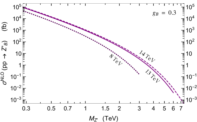
Figure 1: Cross section for production of a $Z^{\prime}_{B}$ boson in proton-proton collisions at $\sqrt{s}=14$, 13 and 8 TeV. The coupling is fixed here at $g_{{}_{B}}=0.3$; the cross section scales as $g_{{}_{B}}^{2}$. Next-to-leading order QCD corrections are included through MadGraph_aMC@NLO.

The most stringent collider limits on the coupling for $M_{Z^{\prime}}<450$ GeV are set by LHC searches for a dijet resonance produced in association with an initial state jet, photon or a leptonically-decaying $W$ boson. The production cross sections for $Z^{\prime}_{B}j$ and $Z^{\prime}_{B}\gamma$ at the 13 TeV LHC, computed at NLO with MadGraph_aMC@NLO, are shown in the left-hand panel of Figure 2 for two choices of the $p_{T}$ cut on the initial state radiation (ISR). The $Z^{\prime}_{B}W$ production cross section times the $W$ branching fraction into leptonic final states (excluding $\tau\nu$) is given in the right-hand panel of Figure 2, by the dashed gray line.

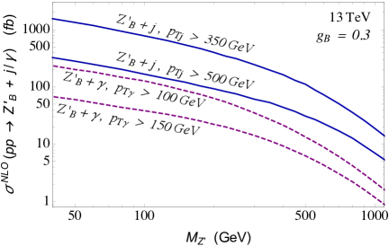
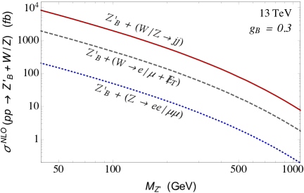
Figure 2: Next-to-leading order cross section for a $Z^{\prime}_{B}$ boson produced at the 13 TeV LHC in association with a jet (solid blue lines) or photon (dashed purple lines) of transverse momentum above a certain limit (left panel), or with a weak boson decaying to jets or leptons (right panel). The coupling used here is $g_{{}_{B}}=0.3$; all cross sections scale as $g_{{}_{B}}^{2}$.

We point out that additional processes that can be used in future searches at low dijet mass involve initial state radiation of a $W$ or $Z$ boson decaying hadronically. The cross section for $Z^{\prime}_{B}$ production in association with an electroweak boson that decay into jets is shown by the solid red line in the right-hand panel of Figure 2. Note that at low mass this rate is larger by a factor of about 5 than the $Z^{\prime}_{B}j$ rate with $p_{Tj}>350$ GeV, so searches for associated $Z^{\prime}_{B}\,W/Z$ production appear promising. The $Z^{\prime}_{B}Z$ production cross section times the sum of $Z$ branching fractions into $e^{+}e^{-}$ and $\mu^{+}\mu^{-}$ is also given in the right-hand panel of Figure 2 (see the dotted blue line). The low background for events with a leptonically-decaying $Z$ and a $jj$ resonance would allow the use of $Z^{\prime}_{B}Z$ production to improve the sensitivity to lower dijet masses.

Using an ISR jet as a trigger for light dijet resonances has been a key aspect for the current search sensitivity at low masses [8, 9, 10]. As a practical matter, however, the large boost to the $Z^{\prime}_{B}$ resonance necessitates the use of jet substructure techniques to both remove contamination from pile-up and distinguish the $Z^{\prime}_{B}$ peak signal from the overwhelming QCD background. The $p_{T}$ requirement from the ISR jet [8, 9, 10] thus leads to a sculpted invariant mass distribution, necessitating the use of novel experimental techniques to decorrelate the $p_{T}$ of the ISR jet from the differential mass distribution [34].

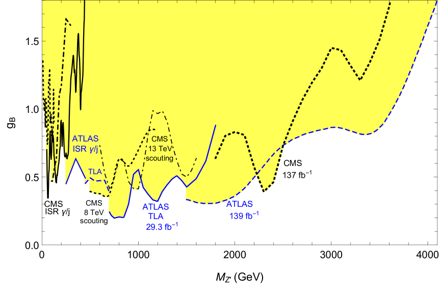
Figure 3: Limits on the $Z^{\prime}_{B}$ boson in the coupling-mass plane, based on the ATLAS and CMS searches [7, 8, 12, 20, 14, 15, 16, 22, 23] described in the text. The yellow shaded region is excluded at the 95% confidence level. The normalization of the $g_{{}_{B}}$ coupling used here is given in Eq. (2.1).

The current coupling-mass limits are shown in Figure 3, and are derived from various types of hadron collider searches, depending on the resonance mass. Only searches that set the most stringent limits for some mass range are included there [7, 8, 12, 20, 14, 15, 16, 22, 23]. Earlier limits that have been superseded can be found in [4].

For $M_{Z^{\prime}}>1.5$ TeV, the most stringent limits on $g_{{}_{B}}$ are set by dijet resonance searches at $\sqrt{s}=13$ TeV. The CMS search [23] is based on the full Run 2 luminosity, totaling 137 fb^-1 of data (which supersedes the earlier high-mass results [20, 21]). The ATLAS search [22] is also based on the full Run 2 luminosity, totaling 139 fb^-1 of data.

These limits assume that the dijet signal is given by the $Z^{\prime}_{B}$ production cross section times the branching fraction $B\!\left(Z^{\prime}_{B}\to jj\right)$ given in Eq. (2.2). In practice, for $M_{Z^{\prime}}\gg 2m_{t}$ there is an additional contribution from $Z^{\prime}_{B}\to t\bar{t}$ because each top quark is highly boosted and may appear as a jet. This effect is weaker in the case of ATLAS searches, where the jet cone size is $R=0.5$, significantly smaller than the one used in CMS dijet searches, $R=1.1$. The $t\bar{t}$ invariant mass distribution matches the dijet one only when both top quarks decay hadronically, otherwise the neutrinos shift the invariant mass below $M_{Z^{\prime}}$. Thus, the effective dijet branching fraction of $Z^{\prime}_{B}$ is slightly higher than 5/6, reaching $5/6+B(W\to jj)^{2}/6\approx 0.91$ at very high masses. Consequently, the limits on $g_{{}_{B}}$ may be up to 5% tighter than those shown in Figure 3.

For 450 GeV $<M_{Z^{\prime}}<1.5$ TeV, there is competition between four searches. The CMS method in that mass range, called “scouting”, uses dijets reconstructed from calorimeter information in the trigger. The latest CMS search of this type uses 27 fb^-1 of 13 TeV data (the low-mass result of [20]) and sets a competitive limit especially in the 0.9–1 TeV mass range, while the search with 18.8 fb^-1 of 8 TeV data [7] still sets the most stringent limit in the 500–700 GeV mass range. The similar ATLAS “Trigger-Level Analysis” (TLA) used 29.3 fb^-1 of 13 TeV data [12], setting the most stringent limit in the 700–900 GeV and 1–1.5 TeV mass ranges; a version of that search [12] with a different event selection and only 3.4 fb^-1 sets the most stringent limit in the 450–500 GeV mass range.

In the 237–450 GeV mass range, the best limits are set by the ATLAS searches with initial state radiation (ISR) of a jet or a photon (79.8 fb^-1 at 13 TeV [14]) and $b$-tagged jets. The ATLAS 139 fb^-1 search using an ISR $W$ boson giving a high-$p_{T}$ lepton for the trigger [35] gives a slightly weaker bound.

Finally, for 50–237 GeV, the limit is set for most $Z^{\prime}_{B}$ masses by the CMS search for a dijet resonance plus an ISR jet with 35.9 fb^-1 accumulated in 2016 [16], where the dijet system is boosted and merged into a single jet with substructure. In the relatively narrow 100–135 GeV mass range, the strongest limit is set by the similar CMS search with the 2015 data of 2.7 fb^-1 [8]. From 10–50 GeV, the CMS analysis with an ISR photon with 35.9 fb^-1 [15] gives the leading direct constraint on dijet resonances.

The coupling-mass plot of Figure 3 shows that there is a gap in sensitivity for $M_{Z^{\prime}}$ roughly in the 200–500 GeV range. Improved techniques will be required to fill that gap. By contrast, the high-mass region will continue to be covered by existing analyses applied to larger data sets. Higher-energy proton-proton colliders will substantially increase the reach at high $M_{Z^{\prime}}$ [36].

At the other end of the plot, masses below 100 GeV are also constrained by electroweak precision and quarkonium measurements. We will next derive these constraints by calculating the mixing of the $Z^{\prime}$ with SM states.

3 $Z^{\prime}_{B}$ mixing with the $Z$ and the photon

Besides the limits from hadron collider searches discussed in the previous Section, there are constraints on the $Z^{\prime}_{B}$ boson from measurements of the $Z$ boson properties. The mixing between the SM $Z$ boson (labelled here $Z_{\rm SM}$) and the $Z^{\prime}_{B}$ boson may modify the branching fractions of the observed $Z$ boson compared to the SM predictions at a level incompatible with existing measurements. Furthermore, the $Z^{\prime}_{B}-Z_{\rm SM}$ mixing as well as the kinetic mixing between the $Z^{\prime}_{B}$ and the photon lead to $Z^{\prime}_{B}$ decays into pairs of leptons [30], which are constrained by searches for dilepton resonances.

A kinetic mixing between the SM hypercharge gauge boson and the $Z^{\prime}_{B}$ may in principle be present at tree level. If, however, the $U(1)_{Y}$ or the $U(1)_{B}$ gauge groups are embedded in a non-Abelian structure at some high scale (which is generically expected as they are not asymptotically free), then the tree-level kinetic mixing vanishes.

Nevertheless, a $Z^{\prime}_{B}-Z_{\rm SM}$ mixing will be generated by loops involving fields that couple to both bosons. To compute the 1-loop $Z^{\prime}_{B}-Z_{\rm SM}$ mixing, we first need to specify all the fields that carry electroweak charges and also couple to $Z^{\prime}_{B}$.

3.1 Kinetic mixing

Let us consider in what follows the theory where $Z^{\prime}_{B}$ is the gauge boson associated with a $U(1)_{B}$ gauge symmetry, so that $Z^{\prime}_{B}$ does not couple to leptons while its couplings given in Eq. (2.1) arise when all SM quarks carry the same $U(1)_{B}$ charge, chosen to be 1/3. The gauge theory with these quark charges is not self-consistent unless certain new fermions, called anomalons, are present to cancel the gauge anomalies. If some of these have masses below $M_{Z^{\prime}}/2$, then the $Z^{\prime}_{B}$ can decay into anomalon pairs, leading to interesting collider signatures [29].

We focus on sets of anomalons which together with the SM quarks satisfy the orthogonality condition Tr$(YB)=0$, where the trace is over all fields, $Y$ is the hypercharge, and $B$ is the $U(1)_{B}$ charge. More explicitly, the condition is

$$\sum_{f=\rm quarks,\;anom.}\!N_{f}\left(Y_{L}^{f}B_{L}^{f}+Y_{R}^{f}B_{R}^{f}\right)=0~{}~{},$$ (3.1)

where the sum is over the fermions $f$, which are all the anomalons and the SM quarks in the gauge eigenstate basis, $Y_{L}^{f}$ and $B_{L}^{f}$ are the hypercharge and $U(1)_{B}$ charge, respectively, of the left-handed $f$ fermion, and $Y_{R}^{f}$ and $B_{R}^{f}$ are the corresponding charges of the right-handed fermions. The color factor is $N_{f}=3$ when $f$ is a quark, and $N_{f}=1$ when $f$ is a color-singlet fermion. When the above equation is satisfied, the leading 1-loop contribution to the kinetic mixing between the SM hypercharge gauge boson and the $Z^{\prime}_{B}$ vanishes, so the constraint from $Z$ measurements is weak.

Kinetic mixing operators are still generated at one loop due to the mass differences between anomalons and SM quarks. The leading operators of this type [30] have dimension six and involve the SM Higgs doublet, $H$, or the $U(1)_{B}$-breaking scalar $\phi$:

$$\phi^{\dagger}\phi\,Z^{\prime}_{B\mu\nu}B^{\mu\nu}\;\;,\;\;H^{\dagger}H\,Z^{\prime}_{B\mu\nu}B^{\mu\nu}\;\;,\;\;H^{\dagger}\tau^{a}H\,Z^{\prime}_{B\mu\nu}W^{a\mu\nu}~{}~{},$$ (3.2)

where $B^{\mu\nu}$ and $W^{a\mu\nu}$ are the hypercharge and $SU(2)_{W}$ field strengths.

There are also mass mixing operators, which arise at dimension six:

$$H^{\dagger}(D^{\mu}H)\,\phi\,(D_{\mu}\phi^{\dagger})+{\rm H.c.}\;\;,\;\;H^{\dagger}(D^{\mu}H)\phi^{\dagger}(D_{\mu}\phi)+{\rm H.c.}\ .$$ (3.3)

These may arise at one loop, depending on the anomalon charges. Once a Higgs doublet and a $\phi$ scalar are replaced by their VEVs, a $Z^{\prime}_{B}-Z_{\rm SM}$ mass mixing is induced.

As the masses of the $Z^{\prime}_{B}$ and the anomalons may be at or below the weak scale, it is appropriate to compute the mixings of $Z^{\prime}_{B}$ with the $Z_{\rm SM}$ and the photon rather than the ones involving the $SU(2)_{W}\times U(1)_{Y}$ gauge bosons. The Lagrangian terms for these can be written as

$$\frac{1}{2}\,Z_{B}^{\prime\,\mu\nu}\left(\kappa_{Z}\,Z_{\rm SM\mu\nu}-\kappa_{\gamma}F_{\mu\nu}\right)+\Delta M^{2}_{Z^{\prime}Z}Z_{B}^{\prime\,\mu}Z_{\rm SM\mu}~{}~{},$$ (3.4)

where the coefficients $\kappa_{Z}$ and $\kappa_{\gamma}$ are dimensionless and real, and $\Delta M^{2}_{Z^{\prime}Z}$ is a mass squared parameter. The field strengths for $Z^{\prime}_{B}$, $Z_{\rm SM}$ and the photon are canonically normalized, i.e., the tree-level kinetic terms are $(-1/4)(Z_{B}^{\prime\,\mu\nu}Z^{\prime}_{B\mu\nu}+Z^{\mu\nu}_{\rm SM}Z_{\rm SM\mu\nu}+F^{\mu\nu}F_{\mu\nu})$.

The real part of the $Z^{\prime}_{B}-Z_{\rm SM}$ mixing amplitude contains two pieces: a kinetic mixing and a mass mixing. The $Z^{\prime}_{B}-Z_{\rm SM}$ mixing amplitude can be written as $\epsilon_{\mu}(Z^{\prime}_{B})\epsilon_{\nu}(Z){\cal A}^{\mu\nu}_{Z^{\prime}Z}$, with $\epsilon_{\mu}(Z^{\prime}_{B})$ and $\epsilon_{\nu}(Z)$ being the polarization vectors of the two gauge bosons. The real part of ${\cal A}^{\mu\nu}_{Z^{\prime}Z}$ is

$${\rm Re}\,{\cal A}^{\mu\nu}_{Z^{\prime}Z}=\kappa_{Z}\left(g^{\mu\nu}p^{2}-p^{\mu}p^{\nu}\right)+\Delta M^{2}_{Z^{\prime}Z}\,g^{\mu\nu}~{}~{},$$ (3.5)

where $p^{\mu}$ is the 4-momentum of the $Z^{\prime}_{B}$ or $Z_{\rm SM}$ bosons.

The sine and cosine of the weak mixing angle are labelled in what follows by $s_{W}$ and $c_{W}$, while the $SU(2)_{W}$ gauge coupling is $g=e/s_{W}$, where $e$ is the electromagnetic gauge coupling. Expressing the $Z_{\rm SM}$ couplings of the left- and right-handed fermion $f$ (without the $g/c_{W}$ prefactor) in terms of their $T^{3}$ value and hypercharge,

$$g_{L,R}^{f}=c_{W}^{2}T^{3}_{L,R}-s_{W}^{2}Y^{f}_{L,R}~{}~{},$$ (3.6)

we find that the sum of the $Z_{\rm SM}$ couplings over the fermions belonging to an $SU(2)_{W}$ multiplet of size $n$ is proportional to the hypercharge $Y^{f}$ of that representation:

$$\sum_{f\in\,\rm n}g_{L,R}^{f}=-n\,s_{W}^{2}Y^{f}_{L,R}~{}~{}.$$ (3.7)

From Eq. (3.1) then follows an important sum rule:

$$\sum_{f=\rm quarks,\;anom.}N_{f}\left(g_{L}^{f}B_{L}^{f}+g_{R}^{f}B_{R}^{f}\right)=0~{}~{}.$$ (3.8)

If all the SM quarks and anomalons had the same mass, then Eq. (3.8) would have implied that the $Z^{\prime}_{B}-Z_{\rm SM}$ kinetic mixing vanishes at one loop. As the top quark is much heavier than the other SM quarks, the kinetic mixing receives a significant contribution from the SM. The anomalons also contribute to the kinetic mixing, with an amount sensitive to the anomalon masses and also to the anomalon charges. The dependence of the kinetic mixing on the anomalon set has not been recognized in previous work [24, 26, 27, 37, 28]. Similarly, the fact that the loop-induced kinetic mixing is finite has been mostly overlooked (an exception is [30]).

In the Appendix we compute the mixing between $Z_{\rm SM}$ and any $Z^{\prime}$ induced at one loop by any fermions that satisfy an orthogonality relation like (3.8). In this section we are primarily interested in the case where the 4-momentum of the gauge bosons satisfies $p^{2}=M_{Z}^{2}$, so that we can extract limits on the $Z^{\prime}$ from measurements at the $Z$ pole. The 1-loop computations of the mixings are simplified when the anomalon couplings to the Higgs doublet are negligible, i.e., the anomalon masses come entirely from Yukawa couplings to the scalar $\phi$ responsible for spontaneously breaking $U(1)_{B}$. In that situation there are no 1-loop contributions to $\Delta M^{2}_{Z^{\prime}Z}$ because the operators (3.3) cannot be generated either by SM quarks (which do not couple to $\phi$) or by anomalons (which do not couple to $H$). This can also be seen from (LABEL:eq:kappa), which gives $\Delta M^{2}_{Z^{\prime}Z}$ after setting $z^{q}_{L}=z^{q}_{R}$ for the SM quarks and $g_{L}^{f}=g_{R}^{f}$ for the anomalons.

The expansion in (A.10) shows that the loops involving the SM quarks other than the top quark have contributions to the kinetic mixing which are of order $(m_{q}/M_{Z})^{2}$ where $m_{q}$ are the SM quark masses, and thus can be neglected. Hence, the kinetic mixing, given in general in (A.9), becomes a sum over the top quark and anomalon contributions:

$$\kappa_{Z}\simeq\frac{g_{{}_{B}}g}{48\pi^{2}c_{W}}\,\left[\left(\frac{1}{2}-\frac{4}{3}s_{W}^{2}\right){\cal F}(m_{t}^{2}/M_{Z}^{2})+\!\!\sum_{f=\rm anom.}\!\!N_{f}\left(g_{L}^{f}B_{L}^{f}+g_{R}^{f}B_{R}^{f}\right){\cal F}(m_{f}^{2}/M_{Z}^{2})\right],$$ (3.9)

The function ${\cal F}$ is given in Eq. (A.8) of the Appendix, and for $m_{f}\gtrsim M_{Z}$ is well approximated by

$${\cal F}(m_{f}^{2}/M_{Z}^{2})\simeq 2\,\ln\!\left(\frac{m_{f}}{M_{Z}}\right)+\frac{5}{3}-\frac{M_{Z}^{2}}{5\,m_{f}^{2}}~{}~{}.$$ (3.10)

For $m_{f}$ in the interval 100–400 GeV, ${\cal F}(m_{f}^{2}/M_{Z}^{2})$ continuously grows from 1.67 to 4.61.

As mentioned in Section 2, we will focus here on the case where all the anomalons are color singlets ($N_{f}=1$) and heavier than $M_{Z^{\prime}}/2$, where $M_{Z^{\prime}}$ is the mass of the physical particle $Z^{\prime}$. The collider constraints on the anomalons are weak in this case: pair production at LEP II sets a lower limit on the anomalon mass of about 90 GeV, depending on the anomalon decay modes [28]. Using (3.7) and replacing the known quantities in Eq. (3.9) by their numerical values, we find the following expression for the $Z^{\prime}_{B}-Z_{\rm SM}$ kinetic mixing at one loop:

$$\kappa_{Z}\simeq 8.70\times 10^{-4}\,g_{{}_{B}}\left(1-0.417\sum_{f=\rm anom.}\!Y^{f}\!\left(B_{L}^{f}+B_{R}^{f}\right){\cal F}(m_{f}^{2}/M_{Z}^{2})\right)~{}~{}.$$ (3.11)

A minimal set of anomalons which includes only color singlets, cancels all gauge anomalies, and satisfies the trace condition is given by the following $SU(2)_{W}\times U(1)_{Y}\times U(1)_{B}$ representations [28, 29]:

$$L_{L}(2,-1/2,-1)\;\;,\;\;L_{R}(2,-1/2,2)\;\;,\;\;E_{L}(1,-1,2)\;\;,\;\;E_{R}(1,-1,-1)$$

$$N_{L}(1,0,2)\;\;,\;\;N_{R}(1,0,-1)\ .$$ (3.12)

The SM gauge singlet fermions, $N_{L}$ and $N_{R}$, are required to cancel the $U(1)_{B}$ and $[U(1)_{B}]^{3}$ anomalies, but do not contribute to the kinetic mixing. The anomalons acquire mass from the scalar $\phi$, with $U(1)_{B}$ charge $+3$ and whose vacuum expectation value (VEV) $\langle\phi\rangle=v_{\phi}$ breaks the $U(1)_{B}$ symmetry. The corresponding Yukawa interactions

$$-y_{L}\overline{L}_{L}\phi^{*}L_{R}-y_{E}\overline{E}_{L}\phi E_{R}-y_{N}\overline{N}_{L}\phi N_{R}+\text{ H.c.}\ ,$$ (3.13)

set the anomalon masses to be $y_{L}v_{\phi}$, $y_{E}v_{\phi}$, and $y_{N}v_{\phi}$. We assume the dominant mass generation arises from $U(1)_{B}$ breaking, and neglect the possible Yukawa interactions to the SM Higgs doublet. We remark that small Yukawa interactions to the SM Higgs doublet, which are needed to ensure the charged anomalons can decay to SM fermions, are still allowed by $h\to\gamma\gamma$ constraints [38]. If all anomalons have the same mass, $m_{f}\gtrsim 90$ GeV, then

$$\sum_{f=\rm anom.}\!Y^{f}\left(B_{L}^{f}+B_{R}^{f}\right){\cal F}(m_{f}^{2}/M_{Z}^{2})=-2\,{\cal F}(m_{f}^{2}/M_{Z}^{2})$$ (3.14)

and we obtain that this anomalon set gives $\kappa_{Z}/g_{{}_{B}}\simeq 2.1\times 10^{-3}$ for $m_{f}=100$ GeV, and $\kappa_{Z}/g_{{}_{B}}\simeq 3.2\times 10^{-3}$ for $m_{f}=200$ GeV.

3.2 Couplings of the physical bosons

Diagonalizing the kinetic terms of the $Z_{\rm SM}$ and $Z^{\prime}_{B}$ bosons, which include the kinetic mixing shown in (3.4), we find that the mass eigenstate bosons, labelled by $Z$ and $Z^{\prime}$, are

$$Z^{\mu}=\cos\theta\,Z^{\mu}_{\rm SM}+\left(\sin\theta\,\sqrt{1-\kappa_{Z}^{2}}-\kappa_{Z}\cos\theta\right)Z^{\prime\mu}_{B}~{}~{},$$

$$Z^{\prime\mu}=\left(\cos\theta\,\sqrt{1-\kappa_{Z}^{2}}+\kappa_{Z}\sin\theta\right)Z^{\prime\mu}_{B}-\sin\theta\,Z^{\mu}_{\rm SM}~{}~{},$$ (3.15)

where $-\pi/4<\theta<\pi/4$ and

$$\tan 2\theta=\frac{2\kappa_{Z}}{1-2\kappa_{Z}^{2}-M_{Z^{\prime}_{B}}^{2}/M_{Z_{\rm SM}}^{2}}\sqrt{1-\kappa_{Z}^{2}}~{}~{}.$$ (3.16)

The squared masses of the two physical states are

$$M_{Z,Z^{\prime}}^{2}=\frac{1}{2(1-\kappa_{Z}^{2})}\left(M_{Z_{\rm SM}}^{2}+M_{Z^{\prime}_{B}}^{2}\pm\sqrt{\left(M_{Z_{\rm SM}}^{2}-M_{Z^{\prime}_{B}}^{2}\right)^{2}+4\kappa_{Z}^{2}\,M_{Z_{\rm SM}}^{2}M_{Z^{\prime}_{B}}^{2}}\;\right)~{}~{},$$ (3.17)

where the $+$ sign corresponds to $M_{Z}^{2}$ only when $M_{Z_{\rm SM}}\geq M_{Z^{\prime}_{B}}$. Since $\kappa_{Z}\ll 1$, in what follows we drop the terms of order $\kappa_{Z}^{2}$ from Eq. (3.15) and from the prefactor of Eq. (3.17). As the $Z^{\prime}_{B}$ mass may be close to $M_{Z_{\rm SM}}$, we do not yet expand the denominator of Eq. (3.16) or the last term of Eq. (3.17).

As a consequence of mixing, the couplings of the physical $Z$ boson to quarks and leptons are changed compared to the SM ones, given in Eq. (3.6), as follows

$$g_{L,R}^{q}\to\hat{g}_{L,R}^{q}=\left(\cos\theta+\kappa_{Z}\sin\theta\right)\,g_{L,R}^{q}+\sin\theta\;\frac{g_{{}_{B}}c_{W}}{6\,g}~{}~{},$$

$$g_{L,R}^{\ell}\to\hat{g}_{L,R}^{\ell}=\left(\cos\theta+\kappa_{Z}\sin\theta\right)\,g_{L,R}^{\ell}~{}~{}.$$ (3.18)

The couplings of the physical $Z^{\prime}$ boson to quarks are modified compared to those of $Z^{\prime}_{B}$ gauge boson shown in Eq. (2.1), by a charge- and chirality-dependent factor:

$$\cos\theta+(-\sin\theta+\kappa_{Z}\cos\theta)\frac{6g}{g_{{}_{B}}c_{W}}g_{L,R}^{q}~{}~{}.$$ (3.19)

In addition, the $Z^{\prime}_{B}-Z_{\rm SM}$ kinetic mixing induces couplings of $Z^{\prime}$ to leptons:

$$Z^{\prime}_{\mu}\;\frac{g}{c_{W}}(-\sin\theta+\kappa_{Z}\cos\theta)\sum_{\ell}\,\left(g_{L}^{\ell}\,\bar{\ell}_{L}\gamma^{\mu}\ell_{L}+g_{R}^{\ell}\,\bar{\ell}_{R}\gamma^{\mu}\ell_{R}\right)~{}~{}.$$ (3.20)

The kinetic mixing between $Z^{\prime}_{B}$ and the photon, $\kappa_{\gamma}$ as defined in (3.4), also contributes to the $Z^{\prime}$ couplings to leptons. The same computation detailed in the Appendix, but with the $Z$ couplings replaced by the photon ones, gives

$$\kappa_{\gamma}\simeq\frac{g_{{}_{B}}e}{48\pi^{2}}\,\left[-\frac{4}{9}{\cal F}(m_{t}^{2}/M_{Z^{\prime}}^{2})+\!\!\sum_{f=\rm anom.}\!\!Q^{f}\left(B_{L}^{f}+B_{R}^{f}\right){\cal F}(m_{f}^{2}/M_{Z^{\prime}}^{2})\right].$$ (3.21)

This induces additional couplings of $Z^{\prime}_{B}$ to leptons, as studied in Ref. [30].

3.3 Limits from electroweak measurements

Let us focus first on the typical case, where the relative mass splitting of the two gauge bosons is large compared to the kinetic mixing: $|M_{Z^{\prime}_{B}}-M_{Z_{\rm SM}}|\gg\kappa_{Z}M_{Z_{\rm SM}}$. In that case Eq. (3.16) implies $\sin\theta\ll 1$ and, to leading order in $\kappa_{Z}^{2}$,

$$\sin\theta\simeq\frac{\kappa_{Z}}{1-M_{Z^{\prime}}^{2}/M_{Z}^{2}}~{}~{}.$$ (3.22)

Furthermore, the mass difference between the two physical particles in this case is approximately equal to the mass difference of the two gauge bosons: $M_{Z^{\prime}}-M_{Z}\simeq M_{Z^{\prime}_{B}}-M_{Z_{\rm SM}}$ up to corrections of order $(\kappa_{Z}M_{Z_{\rm SM}})^{2}/(M_{Z^{\prime}_{B}}-M_{Z_{\rm SM}})^{2}$. The constraints from $Z$ pole measurements depend on the size of the $M_{Z^{\prime}}-M_{Z}$ mass splitting compared to the measured $Z$ width, $\Gamma_{Z}\approx 2.5$ GeV.

When $|M_{Z^{\prime}}-M_{Z}|\gtrsim\Gamma_{Z}$, the contribution from $Z^{\prime}$ exchange to the $Z$ pole observables can be neglected. In that case, the main effect of the $Z^{\prime}_{B}-Z_{\rm SM}$ kinetic mixing is a relative change in the hadronic $Z$ width compared to the SM prediction:

$$\frac{\Delta\Gamma_{\rm had}(Z)}{\Gamma_{\rm had}^{\rm SM}(Z)} \!=\! \frac{3\left[(\hat{g}_{L}^{d})^{2}+(\hat{g}_{R}^{d})^{2}\right]+2\left[(\hat{g}_{L}^{u})^{2}+(\hat{g}_{R}^{u})^{2}\right]}{3\left[(g_{L}^{d})^{2}+(g_{R}^{d})^{2}\right]+2\left[(g_{L}^{u})^{2}+(g_{R}^{u})^{2}\right]}-1$$ (3.23)

$$\!\simeq\! -\frac{A_{1}\,g_{{}_{B}}\kappa_{Z}}{1-M_{Z^{\prime}}^{2}/M_{Z}^{2}}~{}~{},$$

where the coefficient $A_{1}$ is a function of the weak mixing angle:

$$A_{1}=\left(\frac{c_{W}}{6g}\right)\frac{1+4s_{W}^{2}/3}{5/4-7s_{W}^{2}/3+11s_{W}^{2}/9}\;\approx 0.310~{}~{}~{}.$$ (3.24)

Note that the correction to the leptonic $Z$ width is of order $\sin^{2}\!\theta$ and can be neglected here. For the anomalon set (3.12), with a common mass fixed at $m_{f}=100$ GeV, the constraint becomes

$$\frac{\Delta\Gamma_{\rm had}(Z)}{\Gamma_{\rm had}^{\rm SM}(Z)}\simeq-6.5\times 10^{-4}\frac{g_{{}_{B}}^{2}}{1-M_{Z^{\prime}}^{2}/M_{Z}^{2}}~{}~{}.$$ (3.25)

The value for the hadronic $Z$ width obtained from a fit [39] to the LEP I and SLC data is $\Gamma_{\rm had}(Z)=1.7444\pm 0.0020$ GeV, while the SM prediction is $\Gamma_{\rm had}^{\rm SM}(Z)=1.7411\pm 0.0008$ GeV. The allowed interval for the relative change in the hadronic $Z$ width, at the 95% CL, is

$$-5.3\times 10^{-4}<\frac{\Delta\Gamma_{\rm had}(Z)}{\Gamma_{\rm had}^{\rm SM}(Z)}<4.3\times 10^{-3}~{}~{}.$$ (3.26)

Comparing this interval with Eq. (3.25) leads to the following upper limit on the $U(1)_{B}$ gauge coupling:

$$g_{{}_{B}}<\left\{\begin{array}[]{c}\displaystyle 0.90\left(1-\frac{M_{Z^{\prime}}^{2}}{M_{Z}^{2}}\right)^{\!1/2}\;,\;{\rm for}\;M_{Z^{\prime}}\lesssim M_{Z}-\Gamma_{Z}~{}~{},\\[11.38109pt] \displaystyle 2.6\left(\frac{M_{Z^{\prime}}^{2}}{M_{Z}^{2}}-1\right)^{\!1/2}\;,\;{\rm for}\;M_{Z^{\prime}}\gtrsim M_{Z}+\Gamma_{Z}~{}~{}.\end{array}\right.$$ (3.27)

assuming the anomalon set (3.12) with a common anomalon mass $m_{f}=100$ GeV. For $m_{f}=200$ GeV, the limit on $g_{{}_{B}}$ is multiplied by 0.43. For other anomalon charges or masses, the right-hand side of (3.27) is multiplied by $(2.1\times 10^{-3}g_{{}_{B}}/\kappa_{Z})^{1/2}$, where $\kappa_{Z}$ is given in Eq. (3.11).

When the $Z^{\prime}$ mass is approximately within one $Z$ width from the $Z$ mass, i.e., in the interval 88.7 GeV $\lesssim M_{Z^{\prime}}\lesssim 93.7$ GeV, $Z^{\prime}$ exchange also contributes to processes such as $e^{+}e^{-}\to$ hadrons near the $Z$ pole. In that case the interference between the $Z$ and $Z^{\prime}$ exchange amplitudes leads to corrections of the cross section for $e^{+}e^{-}\to$ hadrons near the $Z$ pole, $\sigma_{\rm had}$, which are not limited to just $\Gamma_{\rm had}(Z)$. The relative change of $\sigma_{\rm had}$ compared to the SM prediction is approximately given by

$$\frac{\Delta\sigma_{\rm had}}{\sigma_{\rm had}^{\rm SM}} \!\simeq\! -\frac{A_{1}\,g_{{}_{B}}\kappa_{Z}}{1-M_{Z^{\prime}}^{2}/M_{Z}^{2}}\left(1+\frac{\Gamma_{Z}\Gamma_{Z^{\prime}}}{4(M_{Z}-M_{Z^{\prime}})^{2}+\Gamma_{Z^{\prime}}^{2}}\right)~{}~{}.$$ (3.28)

To derive this we took the energy of the $e^{+}e^{-}$ collision to be $\sqrt{s}=M_{Z}$. The last term in the parenthesis is due to interference, and depends on the total width of the $Z^{\prime}$ boson: $\Gamma_{Z^{\prime}}\simeq g_{{}_{B}}^{2}M_{Z^{\prime}}/(24\pi)$ to leading order in $\sin\theta$. The fit to the LEP I and SLD data gives $\sigma_{\rm had}=41.541\pm 0.037$ nb, which is 1.6$\sigma$ higher than the SM prediction, $\sigma_{\rm had}^{\rm SM}=41.481\pm 0.008$ nb [39]. As a consequence, the lower limit on $\sigma_{\rm had}$ is particularly tight at the 95% CL:

$$-3.4\times 10^{-4}<\frac{\Delta\sigma_{\rm had}}{\sigma_{\rm had}^{\rm SM}}<3.2\times 10^{-3}\ .$$ (3.29)

Comparing this interval with Eq. (3.28) gives a nonlinear constraint on $g_{{}_{B}}$ as a function of $M_{Z^{\prime}}$, which applies to the $M_{Z}-\Gamma_{Z}\lesssim M_{Z^{\prime}}\lesssim M_{Z}+\Gamma_{Z}$ range except for a very narrow region centered around $M_{Z}$:

$$g_{{}_{B}}^{2}+\left[\left(\frac{1-M_{Z^{\prime}}/M_{Z}}{8.7\times 10^{-3}\,g_{{}_{B}}^{2}}\right)^{\!2}+0.40\right]^{-1}<\,\left\{\begin{array}[]{c}\displaystyle 1.0\left(1-\frac{M_{Z^{\prime}}}{M_{Z}}\right)\,,\;{\rm for}\;\kappa_{Z}\lesssim 1-\frac{M_{Z^{\prime}}}{M_{Z}}\lesssim\frac{\Gamma_{Z}}{M_{Z}}\\[14.22636pt] \displaystyle 9.8\left(\frac{M_{Z^{\prime}}}{M_{Z}}-1\right)\;,\;{\rm for}\;\kappa_{Z}\lesssim\frac{M_{Z^{\prime}}}{M_{Z}}-1\lesssim\frac{\Gamma_{Z}}{M_{Z}}\end{array}\right.\ .$$ (3.32)

(3.33)

Here we used the anomalon set (3.12) with a common mass fixed at $m_{f}=100$ GeV. We will use the above constraint as well as Eq. (3.27) when we extend the coupling-mass plot at low masses in Section 4. For $m_{f}=200$ GeV, the right-hand side of (3.33) must be multiplied by a factor of 0.66, while for other anomalon masses or charges the factor is $2.1\times 10^{-3}g_{{}_{B}}/\kappa_{Z}$.

For $|M_{Z^{\prime}}-M_{Z}|\lesssim\kappa_{Z}\,M_{Z}$, the 1-loop mixing between $Z^{\prime}_{B}$ and $Z_{\rm SM}$ in Eq. (3.16) is large, $\sin\theta\approx 1/\sqrt{2}$, as also discussed in Ref. [40]. Because the diagonalization to the mass basis considers only the pole terms in the 1-loop wavefunction correction, the evaluation of the 1-loop diagrams cannot be neglected in scattering cross sections. The mass shift of the $Z_{\rm SM}$ boson from a $Z^{\prime}$ close in mass was used before as the constraint on $\kappa_{Z}$ [41], but that result needs to be revisited for the very narrow region where the relative mass difference is below $\kappa_{Z}$. In particular, the 1-loop interference in scattering processes with $|M_{Z^{\prime}}-M_{Z}|\lesssim\kappa_{Z}\,M_{Z}$ leads to interesting new phenomenology akin to neutral meson mixing, which we reserve for future study.

4 Low-mass constraints in the minimal $Z^{\prime}_{B}$ model

The coupling-mass plot is very useful for displaying the LHC dijet resonance limits. Its linear-linear version (see Figure 3), however, does not clearly show the limits for new bosons at or below the electroweak scale.

By contrast, the log-log version of the coupling-mass plot, shown in Figure 4, clearly displays the low mass region. The yellow-shaded region is excluded at the 95% confidence level by dijet resonance searches at the LHC (and is identical to the shaded region from Figure 3). The gray-shaded region labelled “$Z$ width” is ruled out by measurements of the hadronic $Z$ width, which would be modified by the $Z$–$Z^{\prime}_{B}$ mixing induced at one loop by the SM quarks and also by the anomalons. The boundary of that region is the limit on the $Z^{\prime}_{B}$ coupling, $g_{{}_{B}}$, given in (3.27) for a common anomalon mass of 100 GeV. The limit is more complicated [see (3.33) and the text after that] when $|M_{Z^{\prime}}-M_{Z}|\lesssim\Gamma_{Z}$, due to interference effects in the cross section for $e^{+}e^{-}\to$ hadrons.

The gray-shaded region labelled “$\Upsilon\to jj$” in Figure 4 is excluded by the search for non-electromagnetic decays of $\Upsilon$ into a jet pair performed by the ARGUS Collaboration [42]. This constraint is based on the ratio $R_{\Upsilon}=\Gamma(\Upsilon\to\text{ hadrons})/\Gamma(\Upsilon\to\mu^{+}\mu^{-})$, which was constrained by ARGUS to be below 2.1. The shape of this exclusion limit has been derived in [27, 28].

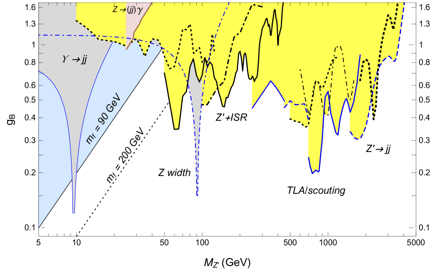
Figure 4: Limits on the $Z^{\prime}_{B}$ boson in the log-log coupling-mass plane. The yellow-shaded region is excluded at the 95% confidence level by dijet resonance searches at the LHC (see Figure 3). The gray-shaded regions (which are particularly strong near 91.2 GeV and 9.5 GeV) are excluded by measurements of the $Z$ hadronic width at LEP I, and by the ARGUS search for non-electromagnetic $\Upsilon$ decay into a jet pair. The blue-shaded region (above the solid straight line) is ruled out by the lower limit on anomalon masses in conjunction with the theoretical upper limit on Yukawa couplings, and the dotted straight light indicates the possible exclusion if the anomalon mass constraint is increased to 200 GeV. The pink-shaded region labelled $Z\to jj\gamma$ is excluded by the L3 search for $Z\to Z^{\prime}\gamma\to jj\gamma$.

In addition to limits from direct dijet resonance searches aimed at the $Z^{\prime}_{B}$ boson, and indirect constraints from $Z$–$Z^{\prime}_{B}$ mixing and $\Upsilon$ decays, we also have constraints on the anomalons, which are required for self-consistency of the theory. One could introduce anomalons which replicate an entire generation of SM fermions, but assign the new quarks $U(1)_{B}$ charge $-1$. The new fermions cancel the $[SU(2)_{W}]^{2}\times U(1)_{B}$ and $[U(1)_{Y}]^{2}\times U(1)_{B}$ anomalies, which are linear in the $U(1)_{B}$ charges, and also avoid generating new $U(1)_{B}$-gravity or $[U(1)_{B}]^{3}$ anomalies [43]. Phenomenologically, however, this solution is ruled out by the observed SM-like behavior of the 125 GeV Higgs boson, because the anomalons behave as a fourth generation of chiral fermions, which exhibit non-decoupling behavior in loop-induced Higgs processes. While additional states can in principle cancel these contributions [44], the non-decoupling nature of the anomalons in Higgs physics combined with the direct production probes for new quarks essentially excludes this solution. This discussion generalizes to any solution where the anomalons are chiral under the SM gauge group.

A better option is to make the anomalons vectorlike under the SM gauge group and chiral under $U(1)_{B}$. Because the only mixed anomalies from SM fields are $[SU(2)_{W}]^{2}U(1)_{B}$ and $[U(1)_{Y}]^{2}U(1)_{B}$, the new anomalons do not have to carry color [45, 46, 47, 48, 49, 50, 51], which significantly weakens their direct production rates at the LHC. Conversely, the anomalons do carry electric charge and hence mediate a non-decoupling diphoton partial width for the scalar associated with $U(1)_{B}$ breaking, which we will explore in a further publication.

An extra feature for hadronic $Z^{\prime}_{B}$ gauge bosons is the possible 1-loop vanishing of $Z$–$Z_{B}^{\prime}$ mixing at the anomalon mass scale, which amounts to a trace condition of all fermions charged under both groups, Tr$(z_{B}Y)=0$, with $z_{B}$ being the charges under $U(1)_{B}$. At energy scales below the anomalon masses, $Z$–$Z^{\prime}_{B}$ mixing is reintroduced logarithmically.

The blue-shaded region in Figure 4 is ruled out by the direct searches for the minimal model anomalons from LEP [28]. We assume a perturbativity limit on the anomalon Yukawa couplings of $y_{L}$, $y_{E}$, $y_{N}\lesssim 4\pi/3$, which then dictates a maximum anomalon mass in the $g_{{}_{B}}$ versus $M_{Z^{\prime}}$ plane, since $v_{\phi}=2M_{Z^{\prime}}/(3g_{{}_{B}})$. Since $L_{L}$ and $L_{R}$ are electroweak doublets, they can be produced directly at colliders by Drell-Yan and electroweak processes. If their charged components are slightly heavier than the neutral components, they decay into soft pions and missing transverse energy [28], a very difficult signature for the LHC. We thus adopt the LEP constraint that anomalons must be heavier than $90$ GeV.

As discussed in [52] and emphasized recently in [53, 54, 55, 56, 57, 38], the $Z$ boson can decay to $Z^{\prime}$ and a photon via a Wess-Zumino-Witten interaction from the non-zero anomaly induced by the non-decoupling effects of the anomalons as they become heavy. The full calculation of the partial width is found in Ref. [38], where the physics of the anomalons and the matching to the Wess-Zumino-Witten term is manifest.

From Ref. [38], the decay width of $Z\to Z^{\prime}_{B}\gamma$ is

$$\Gamma(Z\to Z^{\prime}_{B}\gamma) =\dfrac{\alpha_{\text{EM}}\alpha\alpha_{B}}{384\pi^{2}c_{W}^{2}}\dfrac{m_{Z}^{\prime 2}}{m_{Z}}\left(1-\dfrac{m_{Z^{\prime}}^{4}}{m_{Z}^{4}}\right)$$

$$\Bigg{|}-\sum\limits_{f\in\text{ SM }}T_{3}(f)Q_{f}^{e}\left[\dfrac{m_{Z}^{2}}{m_{Z}^{2}-m_{Z^{\prime}}^{2}}\left(B_{0}(m_{Z}^{2},m_{f})-B_{0}(m_{Z^{\prime}}^{2},m_{f})\right)+2m_{f}^{2}C_{0}(m_{f})\right]$$

$$+3\left(\dfrac{m_{Z}^{2}}{m_{Z}^{2}-m_{Z^{\prime}}^{2}}\left(B_{0}(m_{Z}^{2},M)-B_{0}(m_{Z^{\prime}}^{2},M)\right)+2M^{2}\dfrac{m_{Z}^{2}}{m_{Z^{\prime}}^{2}}C_{0}(M)\right)\Bigg{|}^{2}\ ,$$ (4.1)

where $T_{3}(f)=+1$ for up-type quarks and $-1$ for down-type quarks, $M$ is the mass of the anomalons and assumed to arise only from $U(1)_{B}$ breaking, and $C_{0}$ and $B_{0}$ are the usual Passarino-Veltman 3-pt. and 2-pt. scalar integrals, following the conventions of Package-X [58, 59],

$$B_{0}(m_{V}^{2},m)\equiv B_{0}(m_{V}^{2},m,m)\ ,\quad C_{0}(m)\equiv C_{0}(0,m_{Z}^{2},m_{Z}^{\prime 2},m,m,m)\ .$$ (4.2)

We can construct an approximate expression for Eqn (4.1) by taking the first five SM quarks to be massless while the top quark and anomalons are taken to infinity. Note this expression is still only valid when the anomalon masses are solely generated from $U(1)_{B}$ breaking. The approximate partial width is then

$$\Gamma(Z\to Z^{\prime}_{B}\gamma) \approx\dfrac{\alpha_{\text{EM}}\alpha\alpha_{B}}{384\pi^{2}c_{W}^{2}}\frac{m_{Z^{\prime}}^{2}}{m_{Z}}\left(1-\frac{m_{Z^{\prime}}^{4}}{m_{Z}^{4}}\right)\left|\frac{3m_{Z}^{2}}{m_{Z^{\prime}}^{2}}-\frac{2}{3}-\frac{7}{3}\frac{m_{Z}^{2}}{m_{Z}^{2}-m_{Z^{\prime}}^{2}}\log\left(\frac{m_{Z}^{2}}{m_{Z^{\prime}}^{2}}\right)\right|^{2}\ .$$ (4.3)

We show the corresponding limit from the L3 search for the exotic $Z$ decay, $Z\to Z^{\prime}\gamma$, $Z^{\prime}\to jj$ [60], also taken from Ref. [38]. The exotic decay constraint by L3 is competitive with the 35.9 fb^-1 ISR $\gamma$ search by CMS [15], although the indirect bound for charged anomalons still provides the dominant constraint [28].

5 Conclusions

We have analyzed the current state of the experimental collider searches for dijet resonances, and compared them with the electroweak constraints on a $Z^{\prime}$ boson. Notably, the LHC experiments now provide the leading constraints not only at masses of several TeV, but also on electroweak scale dijet resonances, thanks to the advent of new trigger pathways and advanced data reconstruction methods.

In addition, the ATLAS and CMS experiments are also placing direct dijet bounds on resonances below 100 GeV, where legacy measurements from LEP experiments, constraints from $\Upsilon$ measurements, and indirect limits on charged anomalons compete for the strongest sensitivity. We have emphasized that in gauged $U(1)_{B}$ models where the fermion sector obeys the orthogonality condition in Eq. (3.1), the kinetic mixing between SM and $Z^{\prime}$ gauge bosons is finite and only logarithmically sensitive to the anomalon masses. Our summary of collider constraints is shown in Fig. 4, which best illustrates the overlapping bounds below 100 GeV.

We have also emphasized that, like the SM, the underlying chiral structure of the $U(1)_{B}$ symmetry is characterized by a single VEV, and hence the $Z^{\prime}_{B}$, $\phi^{0}$, and anomalon masses cannot be arbitrarily decoupled from each other without violating perturbative unitarity. In the coupling versus mass plane, the improving constraints continue to probe higher scales of $U(1)$ symmetry breaking, as evident from the diagonal lines corresponding to constant $m_{f}$ anomalon masses in Fig. 4. The possible sensitivity improvements from collider searches for anomalons as well as signals of the symmetry breaking sector (see, e.g. Ref. [61]) are left for future work.

Acknowledgments: FY is supported by the Cluster of Excellence PRISMA⁺, “Precision Physics, Fundamental Interactions and Structure of Matter” (EXC 2118/1) within the German Excellence Strategy (project ID 39083149). Fermilab is administered by Fermi Research Alliance, LLC under Contract No. DE-AC02-07CH11359 with the U.S. Department of Energy, Office of Science, Office of High Energy Physics.

Appendix:  $Z^{\prime}-Z$ mixing

In this Appendix we compute the kinetic and mass mixings of the gauge eigenstate $Z^{\prime}_{\rm g.e.}$ boson with the $Z_{\rm SM}$ boson, for general couplings ($z^{f}\,$) of $Z^{\prime}_{\rm g.e.}$ to the fermions that satisfy the orthogonality relation Tr$(Yz)=0$, where $Y$ is the hypercharge.

The 1-loop amplitude for $Z^{\prime}_{\rm g.e.}-Z_{\rm SM}$ mixing induced by fermions is given by $\epsilon_{\mu}\epsilon_{\nu}{\cal A}^{\mu\nu}$, where $\epsilon_{\mu},\epsilon_{\nu}$ are the polarization vectors of the two gauge bosons, and

$${\cal A}^{\mu\nu} \!\!=\!\! i\,\frac{g_{{}_{B}}g}{c_{W}}\mu^{4-D}\int\!\!\frac{d^{D}k}{(2\pi)^{D}}\sum_{f}\frac{N_{f}}{\left[(p+k)^{2}-m_{f}^{2}\right]\left(k^{2}-m_{f}^{2}\right)}\left\{m_{f}^{2}\left(g_{L}^{f}z_{R}^{f}+g_{R}^{f}z_{L}^{f}\right)g^{\mu\nu}\right.$$ (A.1)

$$+\left.\left(g_{L}^{f}z_{L}^{f}+g_{R}^{f}z_{R}^{f}\right)\left[p^{\mu}k^{\nu}+k^{\mu}p^{\nu}+2k^{\mu}k^{\nu}-g^{\mu\nu}(p+k)\cdot k\rule{0.0pt}{11.38109pt}\right]\right\}~{}~{}.$$

Here $p$ is the 4-momentum of the $Z^{\prime}_{\rm g.e.}$ and $Z_{\rm SM}$ bosons, and we used dimensional regularization with $D=4-\varepsilon$ and a scale $\mu$. The above sum is over the fermions $f$, which have a color factor $N_{f}$. Their right- and left-handed components ($f_{R}$ and $f_{L}$) carry $Z^{\prime}_{\rm g.e.}$ charges $z^{f}_{R}$ and $z^{f}_{L}$, respectively, and also have couplings ($g^{f}_{R}$ and $g^{f}_{L}$) to the $Z_{\rm SM}$ boson. After combining the denominators, we get

$${\cal A}^{\mu\nu} \!\!=\!\! i\,\frac{g_{{}_{B}}g}{c_{W}}\;\int_{0}^{1}\!dx\,\sum_{f}N_{f}\left\{\rule{0.0pt}{17.07164pt}m_{f}^{2}\left(g_{L}^{f}z_{R}^{f}+g_{R}^{f}z_{L}^{f}\right)g^{\mu\nu}I_{0}^{f}\right.$$ (A.2)

$$+\left.\left(g_{L}^{f}z_{L}^{f}+g_{R}^{f}z_{R}^{f}\right)\left[g^{\mu\nu}I_{1}^{f}+x(1-x)\left(g^{\mu\nu}p^{2}-2p^{\mu}p^{\nu}\right)I_{0}^{f}\right]\rule{0.0pt}{17.07164pt}\right\}~{}~{},$$

where $I_{0}^{f}$ and $I_{1}^{f}$ are the following integrals:

$$\left\{I_{0}^{f}\,,\,I_{1}^{f}\right\}=\mu^{4-D}\int\!\!\frac{d^{D}k}{(2\pi)^{D}}\frac{1}{\left[k^{2}-m_{f}^{2}+x(1-x)p^{2}\right]^{2}}\left\{1\,,\,k^{2}\left(\frac{2}{D}-1\right)\right\}~{}~{}.$$ (A.3)

The orthogonality relation Tr$(Yz)=0$ implies that the fermion charges satisfy

$$\sum_{f}N_{f}\left(g_{L}^{f}z_{L}^{f}+g_{R}^{f}z_{R}^{f}\right)=0~{}~{}.$$ (A.4)

Consequently, the apparent quadratic divergence of $I_{1}^{f}$ in the $D=4$ limit vanishes after the sum over fermions is performed. The usual $\varepsilon$ expansion and the $\overline{\rm MS}$ scheme lead to the following expressions for the integrals:

$$I_{0}^{f}=\frac{-i}{(4\pi)^{2}}\,\ln\left(\frac{m_{f}^{2}}{\mu^{2}}-x(1-x)\frac{p^{2}}{\mu^{2}}-i\epsilon_{0}\right)~{}~{},$$

(A.5)

$$I_{1}^{f}=-\left(m_{f}^{2}-x(1-x)p^{2}\rule{0.0pt}{11.38109pt}\right)I_{0}^{f}~{}~{}~{},$$

where $i\epsilon_{0}$ is the prescription for the complex logarithm when $m_{f}^{2}<x(1-x)p^{2}$.

The real part of the $Z^{\prime}_{\rm g.e.}-Z_{\rm SM}$ mixing amplitude contains two pieces, as shown in Eq. (3.5): a kinetic mixing (with dimensionless coefficient $\kappa_{Z}$), and a mass mixing $\Delta M^{2}_{Z^{\prime}Z}$ (the off-diagonal entry in the mass-squared matrix for the two gauge bosons). From Eq. (A.2) and the second Eq. (A.5) follows that

$$\kappa_{Z} \!=\! 2\,\frac{g_{{}_{B}}g}{c_{W}}\;\sum_{f}N_{f}\left(g_{L}^{f}z_{L}^{f}+g_{R}^{f}z_{R}^{f}\right)\,{\rm Re}\;i\!\int_{0}^{1}\!dx\,x(1-x)I_{0}^{f}~{}~{}~{},$$

$$\Delta M^{2}_{Z^{\prime}Z} \!=\! -\,\frac{g_{{}_{B}}g}{c_{W}}\;\sum_{f}N_{f}\,m_{f}^{2}\left(g_{L}^{f}-g_{R}^{f}\right)\left(z_{L}^{f}-z_{R}^{f}\right)\,{\rm Re}\;i\!\int_{0}^{1}\!dx\,I_{0}^{f}~{}~{}~{}.$$

Integrating over $x$, we find

$$\int_{0}^{1}\!dx\,x(1-x)\,I_{0}^{f}=\frac{-i}{6(4\pi)^{2}}\left[\ln\!\left(\frac{p^{2}}{\mu^{2}}\right)-\frac{5}{3}+{\cal F}(m_{f}^{2}/p^{2})+i\pi\,{\cal G}(m_{f}^{2}/p^{2})\right]~{}.$$ (A.7)

The functions introduced here are ${\cal G}(y)=\theta(1-4y)\,\left(1+2y\right)\sqrt{1-4y}\,$, where $\theta$ is the step function, and

$${\cal F}(y)=\ln y-4y+(1+2y)\,\left|4y-1\rule{0.0pt}{10.81204pt}\right|^{1/2}\!\times\!\left\{\begin{array}[]{c}\displaystyle\ln\!\left(\frac{\displaystyle 1+\!\sqrt{1-4y}}{2y}-1\!\right)\;\,{\rm for}\;\,y\leq\frac{1}{4}~{}~{},\\[14.22636pt] \displaystyle 2\,\arctan\!\left[(4y-1)^{-1/2}\rule{0.0pt}{11.09654pt}\right]\;\,{\rm for}\;\,y>\frac{1}{4}~{}~{}.\end{array}\right.$$ (A.8)

We emphasize that the sum over fermion loops removes not only the quadratic divergence from $I_{1}^{f}$, but also the logarithmically divergent part of each fermion loop, which is shown in (A.7). Thus, the coefficient for kinetic mixing of any $Z^{\prime}_{\rm g.e.}$ and $Z_{\rm SM}$ of 4-momentum $p$ is finite, and can be written as the following sum over the fermion loops:

$$\kappa_{Z} \!\simeq\! \!\frac{g_{{}_{B}}g}{48\pi^{2}c_{W}}\,\sum_{f}\,N_{f}\left(g_{L}^{f}z_{L}^{f}+g_{R}^{f}z_{R}^{f}\right){\cal F}(m_{f}^{2}/p^{2})~{}~{}.$$ (A.9)

This result is used in Section 3. The expansion of the function ${\cal F}(y)$ for $y\ll 1/4$ is

$${\cal F}(y)\simeq-6y+6y^{2}\ln y+O\!\left(y^{2}\right)~{}~{},$$ (A.10)

while for $y\gg 1/4$

$${\cal F}(y)\simeq\ln y+\frac{5}{3}-\frac{1}{5y}+O\!\left((4y)^{-2}\rule{0.0pt}{10.98276pt}\right)~{}~{}.$$ (A.11)

References

- [1]
- [2] T. Han, I. Lewis and Z. Liu, “Colored resonant signals at the LHC: largest rate and simplest topology,” JHEP 1012, 085 (2010) [arXiv:1010.4309 [hep-ph]].
- [3] R. M. Harris and K. Kousouris, “Searches for dijet resonances at hadron colliders,” Int. J. Mod. Phys. A 26, 5005 (2011) [arXiv:1110.5302 [hep-ex]].
- [4] B. A. Dobrescu and F. Yu, “Coupling-mass mapping of dijet peak searches,” Phys. Rev. D 88, no. 3, 035021 (2013) Erratum: [Phys. Rev. D 90, no. 7, 079901 (2014)] [arXiv:1306.2629 [hep-ph]].
- [5] M. Chala, F. Kahlhoefer, M. McCullough, G. Nardini and K. Schmidt-Hoberg, “Constraining dark sectors with monojets and dijets,” JHEP 1507, 089 (2015) [arXiv:1503.05916 [hep-ph]].
- [6] C. Shimmin and D. Whiteson, “Boosting low-mass hadronic resonances,” Phys. Rev. D 94, no. 5, 055001 (2016) [arXiv:1602.07727 [hep-ph]].
- [7] V. Khachatryan et al. [CMS Collaboration], “Search for narrow resonances in dijet final states at 8 TeV with the novel CMS technique of data scouting,” Phys. Rev. Lett. 117, no.3, 031802 (2016) [arXiv:1604.08907 [hep-ex]].
- [8] A. M. Sirunyan et al. [CMS Collaboration], “Search for low mass vector resonances decaying to quark-antiquark pairs in proton-proton collisions at TeV,” Phys. Rev. Lett. 119, no.11, 111802 (2017) [arXiv:1705.10532 [hep-ex]].
- [9] A. M. Sirunyan et al. [CMS Collaboration], “Search for low mass vector resonances decaying into quark-antiquark pairs in proton-proton collisions at TeV,” JHEP 01, 097 (2018) [arXiv:1710.00159 [hep-ex]].
- [10] M. Aaboud et al. [ATLAS Collaboration], “Search for light resonances decaying to boosted quark pairs and produced in association with a photon or a jet in proton-proton collisions at TeV with the ATLAS detector,” Phys. Lett. B 788, 316-335 (2019) [arXiv:1801.08769 [hep-ex]].
- [11] A. M. Sirunyan et al. [CMS Collaboration], “Search for narrow resonances in the b-tagged dijet mass spectrum in proton-proton collisions at 8 TeV,” Phys. Rev. Lett. 120, no.20, 201801 (2018) [arXiv:1802.06149 [hep-ex]].
- [12] M. Aaboud et al. [ATLAS Collaboration], “Search for low-mass dijet resonances using trigger-level jets with the ATLAS detector in collisions at TeV,” Phys. Rev. Lett. 121, no.8, 081801 (2018) [arXiv:1804.03496 [hep-ex]].
- [13] M. Aaboud et al. [ATLAS Collaboration], “Search for resonances in the mass distribution of jet pairs with one or two jets identified as -jets in proton-proton collisions at TeV with the ATLAS detector,” Phys. Rev. D 98, 032016 (2018) [arXiv:1805.09299 [hep-ex]].
- [14] M. Aaboud et al. [ATLAS Collaboration], “Search for low-mass resonances decaying into two jets and produced in association with a photon using collisions at TeV with the ATLAS detector,” Phys. Lett. B 795, 56-75 (2019) doi:10.1016/j.physletb.2019.03.067 [arXiv:1901.10917 [hep-ex]].
- [15] A. M. Sirunyan et al. [CMS Collaboration], “Search for Low-Mass Quark-Antiquark Resonances Produced in Association with a Photon at =13 TeV,” Phys. Rev. Lett. 123, no.23, 231803 (2019) [arXiv:1905.10331 [hep-ex]].
- [16] A. M. Sirunyan et al. [CMS Collaboration], “Search for low mass vector resonances decaying into quark-antiquark pairs in proton-proton collisions at 13 TeV,” Phys. Rev. D 100, no.11, 112007 (2019) [arXiv:1909.04114 [hep-ex]].
- [17] A. M. Sirunyan et al. [CMS Collaboration], “Search for dijet resonances using events with three jets in proton-proton collisions at s=13TeV,” Phys. Lett. B 805, 135448 (2020) [arXiv:1911.03761 [hep-ex]].
- [18] G. Aad et al. [ATLAS Collaboration], “Search for dijet resonances in events with an isolated charged lepton using TeV proton-proton collision data collected by the ATLAS detector,” JHEP 06, 151 (2020) [arXiv:2002.11325 [hep-ex]].
- [19] M. Aaboud et al. [ATLAS Collaboration], “Search for new phenomena in dijet events using 37 fb-1 of collision data collected at 13 TeV with the ATLAS detector,” Phys. Rev. D 96, no.5, 052004 (2017) [arXiv:1703.09127 [hep-ex]].
- [20] A. M. Sirunyan et al. [CMS Collaboration], “Search for narrow and broad dijet resonances in proton-proton collisions at TeV and constraints on dark matter mediators and other new particles,” JHEP 08, 130 (2018) [arXiv:1806.00843 [hep-ex]].
- [21] CMS Collaboration, “Searches for dijet resonances in pp collisions at TeV using the 2016 and 2017 datasets,” report PAS-EXO-17-026, Sept. 2018, https://inspirehep.net/record/1693731.
- [22] G. Aad et al. [ATLAS Collaboration], “Search for new resonances in mass distributions of jet pairs using 139 fb-1 of collisions at TeV with the ATLAS detector,” JHEP 03, 145 (2020) [arXiv:1910.08447 [hep-ex]].
- [23] A. M. Sirunyan et al. [CMS Collaboration], “Search for high mass dijet resonances with a new background prediction method in proton-proton collisions at 13 TeV,” JHEP 05, 033 (2020) [arXiv:1911.03947 [hep-ex]].
- [24] C. D. Carone and H. Murayama, “Possible light U(1) gauge boson coupled to baryon number,” Phys. Rev. Lett. 74, 3122 (1995) [hep-ph/9411256].
- [25] D. C. Bailey and S. Davidson, “Is there a vector boson coupling to baryon number?,” Phys. Lett. B 348, 185 (1995) [hep-ph/9411355].
- [26] C. D. Carone and H. Murayama, “Realistic models with a light U(1) gauge boson coupled to baryon number,” Phys. Rev. D 52, 484 (1995) [hep-ph/9501220].
- [27] A. Aranda and C. D. Carone, “Limits on a light leptophobic gauge boson,” Phys. Lett. B 443, 352 (1998) [hep-ph/9809522].
- [28] B. A. Dobrescu and C. Frugiuele, “Hidden GeV-scale interactions of quarks,” Phys. Rev. Lett. 113, 061801 (2014) [arXiv:1404.3947 [hep-ph]].
- [29] B. A. Dobrescu, “Leptophobic boson signals with leptons, jets and missing energy,” arXiv:1506.04435 [hep-ph].
- [30] B. A. Dobrescu, P. J. Fox and J. Kearney, “Higgs-photon resonances,” Eur. Phys. J. C 77, no. 10, 704 (2017) [arXiv:1705.08433 [hep-ph]].
- [31] J. Alwall et al., “The automated computation of tree-level and next-to-leading order differential cross sections, and their matching to parton shower simulations,” JHEP 1407, 079 (2014) [arXiv:1405.0301 [hep-ph]].
- [32] A. Alloul, N. D. Christensen, C. Degrande, C. Duhr and B. Fuks, “FeynRules 2.0 - A complete toolbox for tree-level phenomenology,” Comput. Phys. Commun. 185, 2250 (2014) [arXiv:1310.1921 [hep-ph]].
- [33] T. Hahn, “Generating Feynman diagrams and amplitudes with FeynArts 3,” Comput. Phys. Commun. 140, 418 (2001) [hep-ph/0012260].
-
[34]
J. Dolen, P. Harris, S. Marzani, S. Rappoccio and N. Tran,
“Thinking outside the ROCs: Designing Decorrelated Taggers (DDT) for jet substructure,”
JHEP 1605, 156 (2016)
[arXiv:1603.00027 [hep-ph]].
C. Shimmin, P. Sadowski, P. Baldi, E. Weik, D. Whiteson, E. Goul and A. Sogaard, “Decorrelated Jet Substructure Tagging using Adversarial Neural Networks,” Phys. Rev. D 96, no. 7, 074034 (2017) [arXiv:1703.03507 [hep-ex]]. - [35] G. Aad et al. [ATLAS Collaboration], “Search for dijet resonances in events with an isolated charged lepton using TeV proton-proton collision data collected by the ATLAS detector,” JHEP 06, 151 (2020) [arXiv:2002.11325 [hep-ex]].
- [36] F. Yu, “Di-jet resonances at future hadron colliders: A Snowmass whitepaper,” arXiv:1308.1077 [hep-ph].
- [37] M. L. Graesser, I. M. Shoemaker and L. Vecchi, “A dark force for baryons,” arXiv:1107.2666 [hep-ph].
- [38] L. Michaels and F. Yu, “Probing new gauge symmetries via exotic decays,” JHEP 03, 120 (2021) [arXiv:2010.00021 [hep-ph]].
- [39] P.A. Zyla et al. [Particle Data Group], “Review of Particle Physics,” PTEP 2020, no.8, 083C01 (2020).
- [40] J. Liu, X. P. Wang and F. Yu, “A tale of two portals: testing light, hidden new physics at future colliders,” JHEP 1706, 077 (2017) [arXiv:1704.00730].
- [41] A. Hook, E. Izaguirre and J. G. Wacker, “Model independent bounds on kinetic mixing,” Adv. High Energy Phys. 2011, 859762 (2011) [arXiv:1006.0973 [hep-ph]].
- [42] H. Albrecht et al. [ARGUS Collaboration], “An upper limit for two jet production in direct decays,” Z. Phys. C 31, 181 (1986).
- [43] P. Fileviez Perez and M. B. Wise, “Baryon and lepton number as local gauge symmetries,” Phys. Rev. D 82, 011901 (2010) Erratum: [Phys. Rev. D 82, 079901 (2010)] [arXiv:1002.1754 [hep-ph]].
- [44] K. Kumar, R. Vega-Morales and F. Yu, “Effects from new colored states and the Higgs portal on gluon fusion and Higgs decays,” Phys. Rev. D 86, 113002 (2012) Erratum: [Phys. Rev. D 87, no. 11, 119903 (2013)] [arXiv:1205.4244 [hep-ph]].
- [45] M. Carena, A. Daleo, B. A. Dobrescu and T. M. P. Tait, “ gauge bosons at the Tevatron,” Phys. Rev. D 70, 093009 (2004) [hep-ph/0408098].
- [46] P. Fileviez Perez and M. B. Wise, “Breaking local baryon and lepton number at the TeV scale,” JHEP 1108, 068 (2011) [arXiv:1106.0343 [hep-ph]].
- [47] M. Duerr, P. Fileviez Perez and M. B. Wise, “Gauge theory for baryon and lepton numbers with leptoquarks,” Phys. Rev. Lett. 110, 231801 (2013) [arXiv:1304.0576].
- [48] M. Duerr and P. Fileviez Perez, “Baryonic Dark Matter,” Phys. Lett. B 732, 101 (2014) [arXiv:1309.3970 [hep-ph]].
- [49] J. M. Arnold, P. Fileviez Perez, B. Fornal and S. Spinner, “B and L at the supersymmetry scale, dark matter, and R-parity violation,” Phys. Rev. D 88, no. 11, 115009 (2013) [arXiv:1310.7052 [hep-ph]].
- [50] P. Fileviez Perez, S. Ohmer and H. H. Patel, “Minimal theory for lepto-baryons,” Phys. Lett. B 735, 283 (2014) [arXiv:1403.8029 [hep-ph]].
- [51] S. Ohmer and H. H. Patel, “Leptobaryons as Majorana dark matter,” Phys. Rev. D 92, no. 5, 055020 (2015) [arXiv:1506.00954 [hep-ph]].
- [52] J. Preskill, “Gauge anomalies in an effective field theory,” Annals Phys. 210, 323 (1991).
- [53] Y. Cui and F. D’Eramo, “Surprises from complete vector portal theories: New insights into the dark sector and its interplay with Higgs physics,” Phys. Rev. D 96, no. 9, 095006 (2017) [arXiv:1705.03897 [hep-ph]].
- [54] J. A. Dror, R. Lasenby and M. Pospelov, “New constraints on light vectors coupled to anomalous currents,” Phys. Rev. Lett. 119, no. 14, 141803 (2017) [arXiv:1705.06726].
- [55] A. Ismail, A. Katz and D. Racco, “On dark matter interactions with the Standard Model through an anomalous ,” JHEP 1710, 165 (2017) [arXiv:1707.00709].
- [56] J. A. Dror, R. Lasenby and M. Pospelov, “Dark forces coupled to nonconserved currents,” Phys. Rev. D 96, no. 7, 075036 (2017) [arXiv:1707.01503 [hep-ph]].
- [57] A. Ismail and A. Katz, “Anomalous and diboson resonances at the LHC,” JHEP 1804, 122 (2018) [arXiv:1712.01840 [hep-ph]].
- [58] H. H. Patel, “Package-X: A Mathematica package for the analytic calculation of one-loop integrals,” Comput. Phys. Commun. 197, 276 (2015) [arXiv:1503.01469]; “Package-X 2.0: A Mathematica package for the analytic calculation of one-loop integrals,” Comput. Phys. Commun. 218, 66 (2017) [arXiv:1612.00009 [hep-ph]].
- [59] G. Passarino and M. J. G. Veltman, “One loop corrections for annihilation into in the Weinberg Model,” Nucl. Phys. B 160, 151-207 (1979)
- [60] O. Adriani et al. [L3 Collaboration], “Isolated hard photon emission in hadronic decays,” Phys. Lett. B 292, 472 (1992).
- [61] M. Duerr, P. F. Perez and J. Smirnov, “Baryonic Higgs at the LHC,” JHEP 1709, 093 (2017) [arXiv:1704.03811 [hep-ph]].